Embed Size (px)
Citation preview
Gene Stru ture Predi tionCourse 2006Lorenzo CeruttiSwiss Institute of Bioinformati s, Lausanne
OutlineIntrodu tionAb initio methodsCoding statisti sSignal dete tionIntegration of signal dete tion and oding statisti sSoftwareHomology methodsPrin iple of the methodSoftwareMixing the methods: de novo methodsPerforman e LC-SIB-2006 � p.1/80
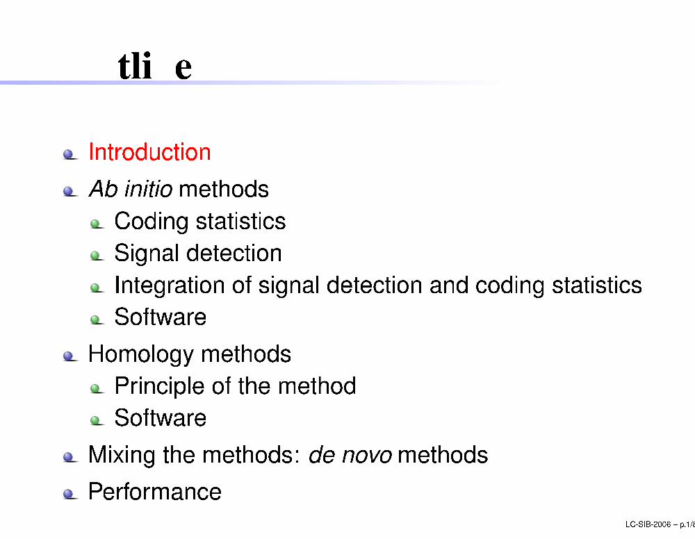
The Central Dogma
LC-SIB-2006 � p.2/80
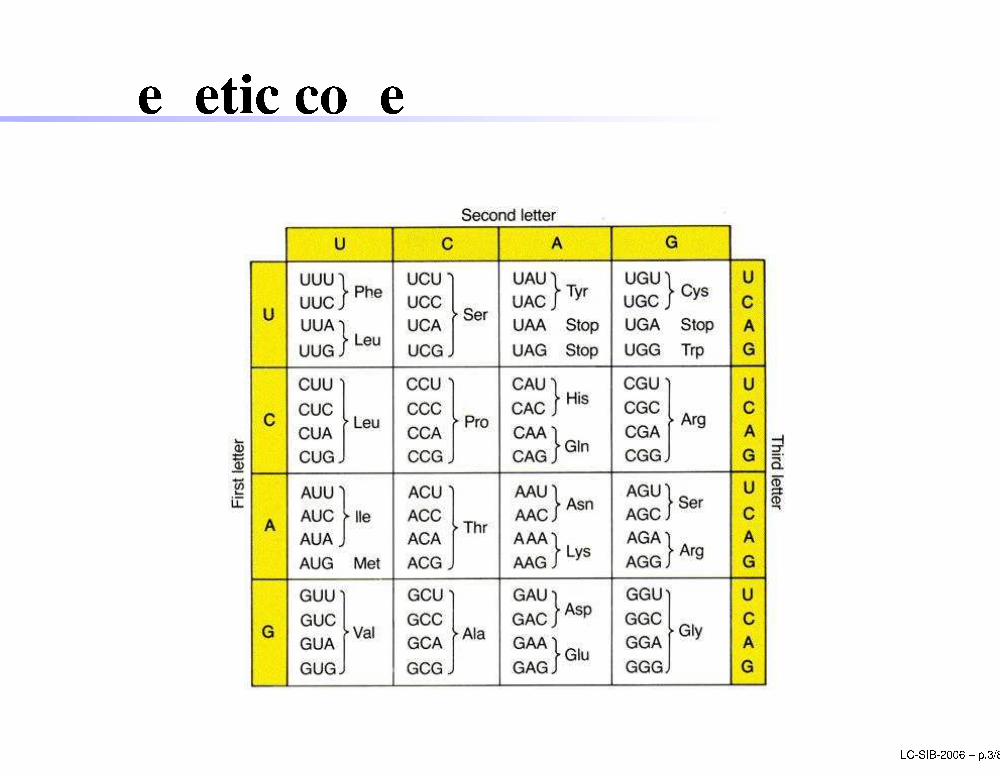
Geneti ode
LC-SIB-2006 � p.3/80
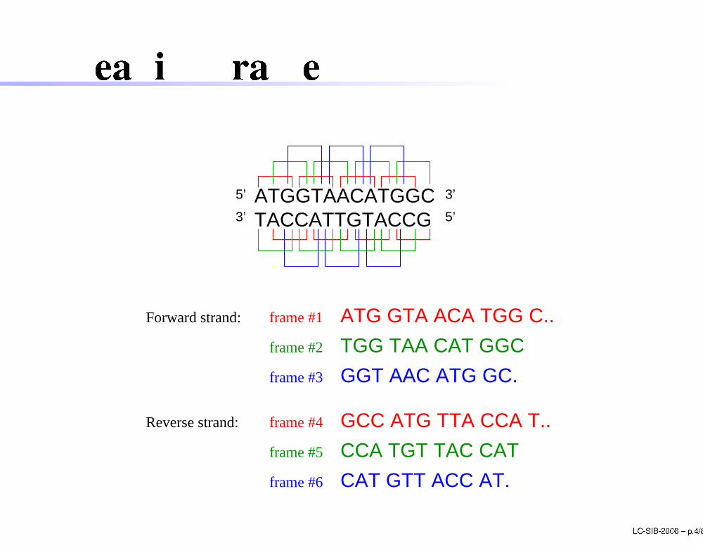
Reading frame
5’ATGGTAACATGGCTACCATTGTACCG
TGG TAA CAT GGC
GGT AAC ATG GC.
ATG GTA ACA TGG C..frame #1
frame #2
frame #3
Forward strand:
Reverse strand: frame #4
frame #5
frame #6
GCC ATG TTA CCA T..
CCA TGT TAC CAT
CAT GTT ACC AT.
5’
3’
3’
LC-SIB-2006 � p.4/80
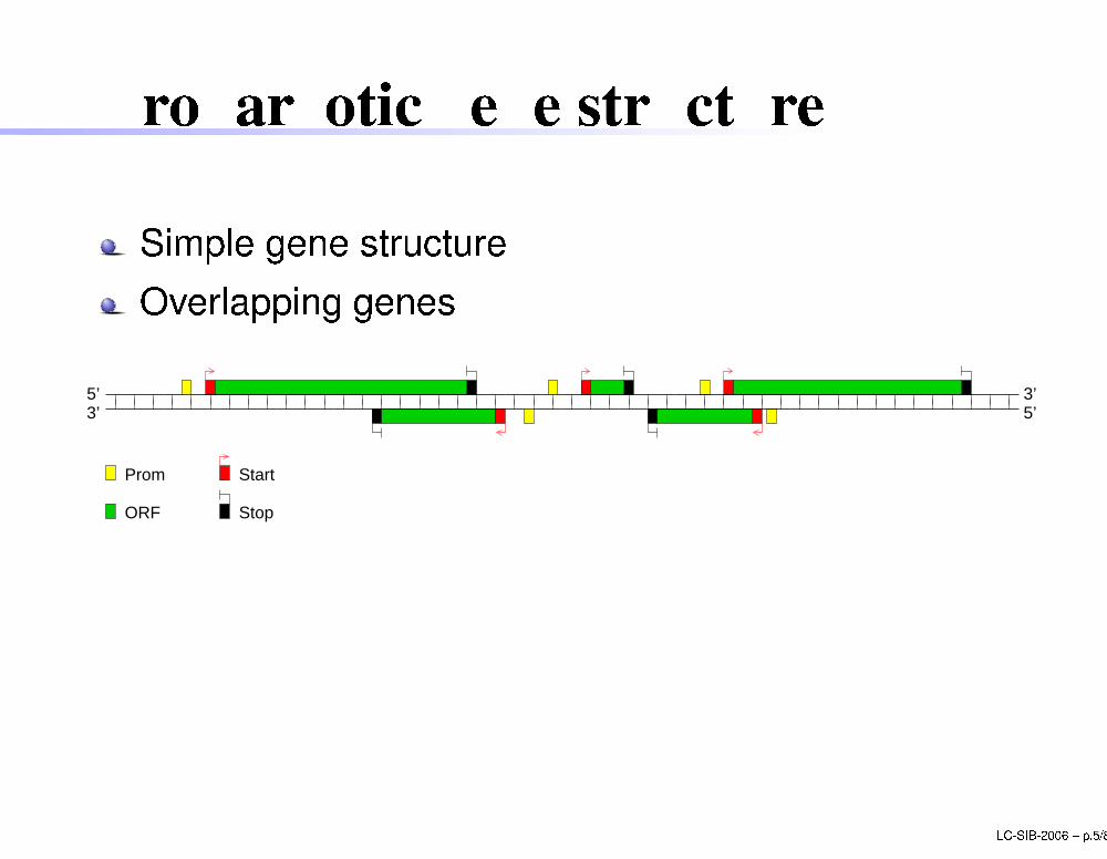
Prokaryoti gene stru ture
Simple gene stru tureOverlapping genes
5’
ORF
Prom Start
Stop
3’5’ 3’
LC-SIB-2006 � p.5/80
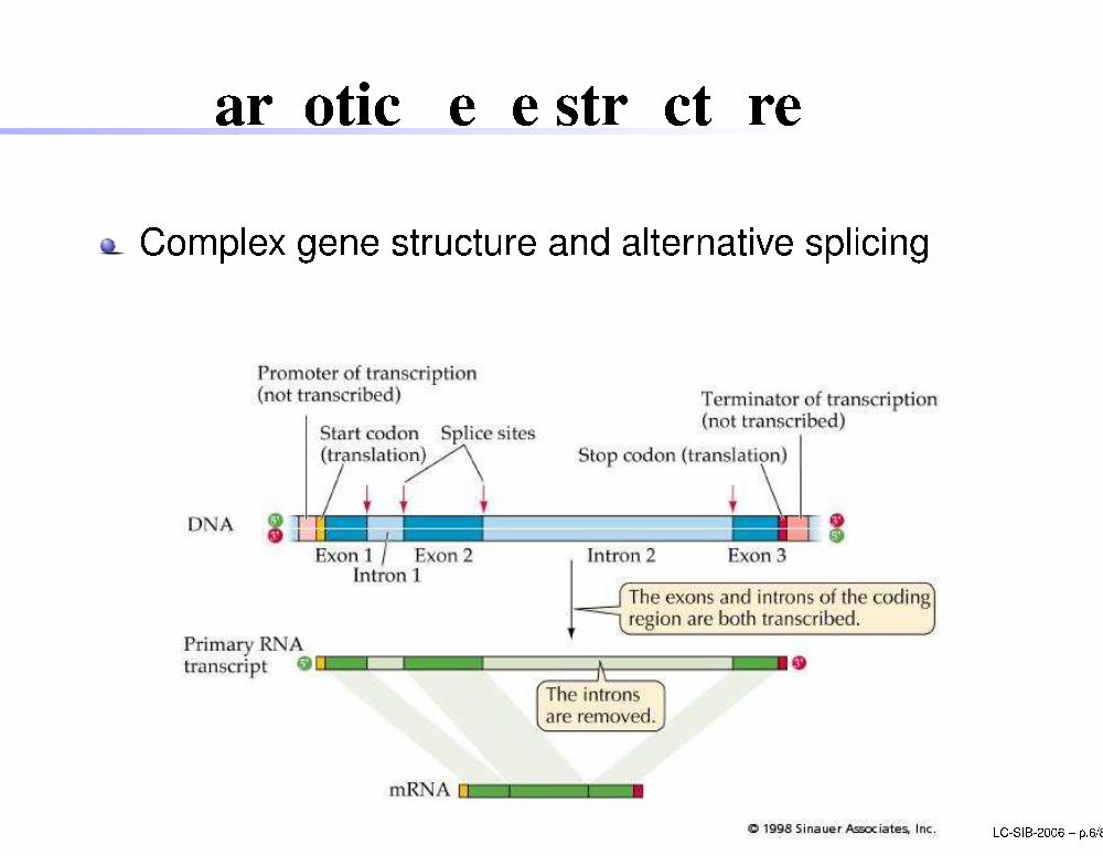
Eukaryoti gene stru ture
Complex gene stru ture and alternative spli ingLC-SIB-2006 � p.6/80
What is gene stru ture predi tion?
Given a genomi DNA sequen e we want to predi tregions oding for a protein: the genes.Gene stru ture predi tion onsists in:identify the oding potential of a region in aparti ular frameidentify boundaries between oding andnon- oding regions
LC-SIB-2006 � p.7/80
Gene predi tion: not an easy task!
DNA sequen e signals have a low information ontentdif� ult to dis riminate real signals from noiseDNA signals may vary in different organismsgene stru ture an be omplex (sparse exons,alternative spli ing, ...)pseudo-genes, selenoproteins, ...sequen e errors (frame shifts, ...)Human genome: �3 billion base pairs and �30,000protein- oding genes
LC-SIB-2006 � p.8/80
Gene stru ture predi tion methods:1
Ab initio methods: oding statisti s: nu leotide ompositional bias in oding regionssignals: short DNA motifs (promoters, start/stop odons, spli e sites, ...)Strength:easy to run and fast exe utiononly require a single genomi sequen e as inputWeakness:prior knowledge is required (training set)high number of mispredi ted stru tures LC-SIB-2006 � p.9/80
Gene stru ture predi tion methods:2
Homology methodsgene stru ture is dedu ed using homologoussequen es from expression data (ESTs, mRNAs,proteins)a urate results when using lose homologoussequen esStrength:a urateWeakness:need of good homologous sequen esslow exe ution LC-SIB-2006 � p.10/80
OutlineIntrodu tionAb initio methodsCoding statisti sSignal dete tionIntegration of signal dete tion and oding statisti sSoftwareHomology methodsPrin iple of the methodSoftwareMixing the methods: de novo methodsPerforman e evaluation LC-SIB-2006 � p.11/80
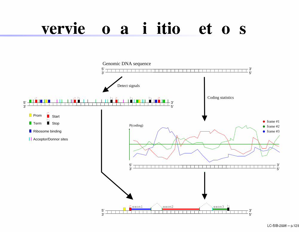
Overview of ab initio methods
P(coding)
frame #3
frame #2
frame #1
3’5’3’
3’
Prom
Term
Ribosome binding
Stop
Start
Acceptor/Donnor sites
5’3’5’
5’
3’5’3’
5’
Genomic DNA sequence
3’
exon3exon2exon1
Detect signals
5’
Coding statistics
3’5’
LC-SIB-2006 � p.12/80
OutlineIntrodu tionAb initio methodsCoding statisti sSignal dete tionIntegration of signal dete tion and oding statisti sSoftwareHomology methodsPrin iple of the methodSoftwareMixing the methods: de novo methodsPerforman e evaluation LC-SIB-2006 � p.13/80
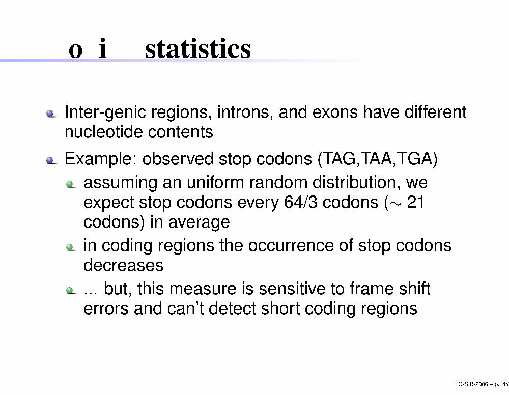
Coding statisti s
Inter-geni regions, introns, and exons have differentnu leotide ontentsExample: observed stop odons (TAG,TAA,TGA)assuming an uniform random distribution, weexpe t stop odons every 64/3 odons (� 21 odons) in averagein oding regions the o urren e of stop odonsde reases... but, this measure is sensitive to frame shifterrors and an't dete t short oding regionsLC-SIB-2006 � p.14/80
Coding statisti s: dimers frequen ies
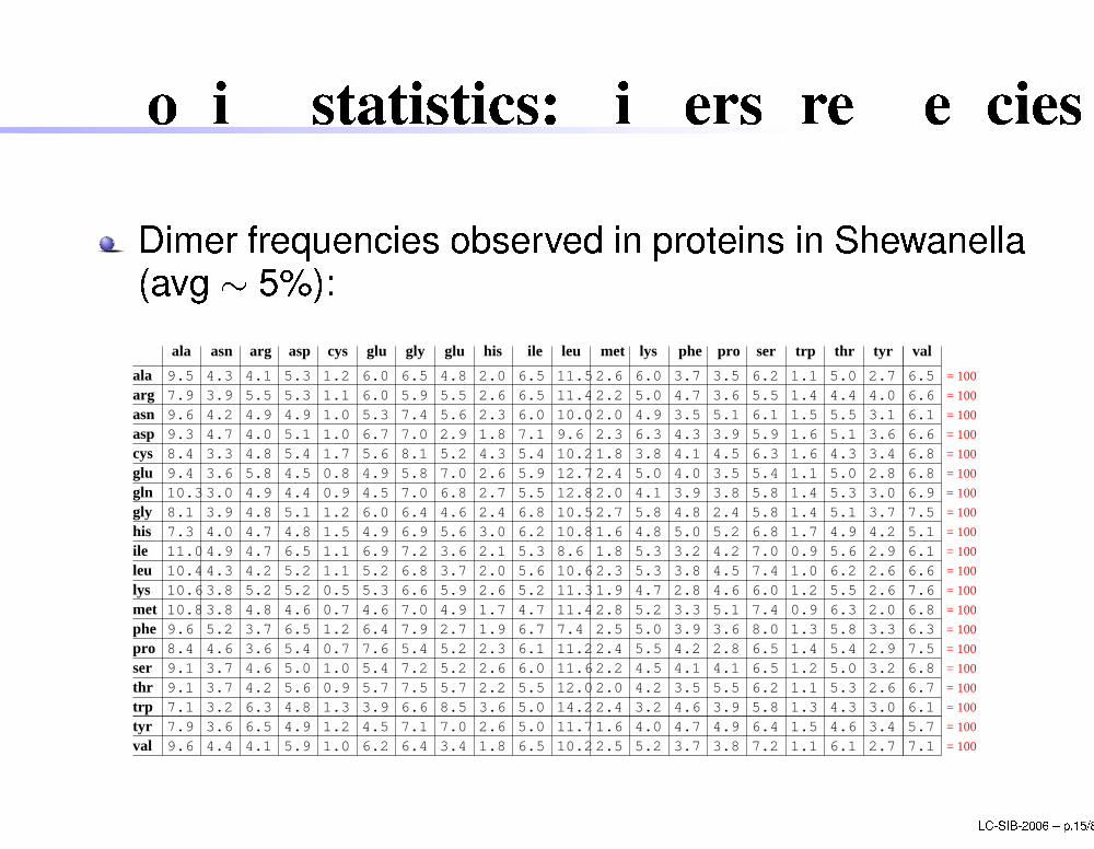
Dimer frequen ies observed in proteins in Shewanella(avg � 5%):3.6
4.94.2 4.9 1.0 5.3 5.67.4 2.3 6.0 10.0 4.92.0 3.5 5.1 6.1 5.51.5 3.1 6.1
8.4 4.83.3 5.4 1.7 5.6 5.28.1 4.3 5.4 10.2 3.81.8 4.1 4.5 6.3 4.31.6 3.4 6.89.4 5.83.6 4.5 0.8 4.9 7.05.8 2.6 5.9 12.7 5.02.4 4.0 3.5 5.4 5.01.1 2.8 6.810.3 4.93.0 4.4 0.9 4.5 6.87.0 2.7 5.5 12.8 4.12.0 3.9 3.8 5.8 5.31.4 3.0 6.98.1 4.83.9 5.1 1.2 6.0 4.66.4 2.4 6.8 10.5 5.82.7 4.8 2.4 5.8 5.11.4 3.7 7.57.3 4.74.0 4.8 1.5 4.9 5.66.9 3.0 6.2 10.8 4.81.6 5.0 5.2 6.8 4.91.7 4.2 5.111.0 4.74.9 6.5 1.1 6.9
9.6
7.2 2.1 5.3 8.6 5.31.8 3.2 4.2 7.0 5.60.9 2.9 6.1
10.6 5.23.8 5.2 0.5 5.3 5.96.6 2.6 5.2 11.3 4.71.9 2.8 4.6 6.0 5.51.2 2.6 7.610.4 4.24.3 5.2 1.1 5.2 3.76.8 2.0 5.6 10.6 5.32.3 3.8 4.5 7.4 6.21.0 2.6 6.6
10.8 4.83.8 4.6 0.7 4.6 4.97.0 1.7 4.7 11.4 5.22.8 3.3 5.1 7.4 6.30.9 2.0 6.89.6 3.75.2 6.5 1.2 6.4 2.77.9 1.9 6.7 7.4 5.02.5 3.9 3.6 8.0 5.81.3 3.3 6.38.4 3.64.6 5.4 0.7 7.6 5.25.4 2.3 6.1 11.2 5.52.4 4.2 2.8 6.5 5.41.4 2.9 7.59.1 4.63.7 5.0 1.0 5.4 5.27.2 2.6 6.0 11.6 4.52.2 4.1 4.1 6.5 5.01.2 3.2 6.89.1 4.23.7 5.6 0.9 5.7 5.77.5 2.2 5.5 12.0 4.22.0 3.5 5.5 6.2 5.31.1 2.6 6.77.1 6.33.2 4.8 1.3 3.9 8.56.6 3.6 5.0 14.2 3.22.4 4.6 3.9 5.8 4.31.3 3.0 6.1
9.6 4.14.4 5.9 1.0 6.2 3.46.4 1.8 6.5 10.2 5.22.5 3.7 3.8 7.2 6.11.1 2.7 7.17.9 6.53.6 4.9 1.2 4.5 7.07.1 2.6 5.0 11.7 4.01.6 4.7 4.9 6.4 4.61.5 3.4 5.7
7.9 5.53.9 5.3 1.1 6.0 5.55.9 2.6 6.5 11.4 5.02.2 4.7 3.6 5.5 4.41.4 4.0 6.6
9.3 4.04.7 5.1 1.0 6.7 2.97.0 1.8 7.1 9.6 6.32.3 4.3 3.9 5.9 5.11.6 3.6 6.6
9.5 4.14.3 5.3 1.2 6.0 4.86.5 2.0 6.5 11.5 6.02.6 3.7 3.5 6.2 5.01.1 2.7 6.5
ala
aspcysgluglnglyhisileleulysmetpheproserthrtrptyrval
asn arg
asn
alaarg
his leu phe pro ser valtyrcys glu gly glu met lys trp thr
= 100
= 100
= 100
= 100
= 100
= 100
= 100
= 100
= 100
= 100
= 100
= 100
= 100
= 100
= 100
= 100
= 100
= 100
= 100
= 100
asp ile
LC-SIB-2006 � p.15/80
Coding statisti s: dimers to di odons
A bias is observed for dimers in proteinsThe dimer bias is re�e ted in di odons: oding andnon- oding regions have different di odons bias.The bias in the observed di odon (hexamer)frequen ies an be used to predi t oding regions ingenomi sequen es.Most of the ab initio methods for gene stru turepredi tion use this information!
LC-SIB-2006 � p.16/80
Coding statisti s: s oring (1)
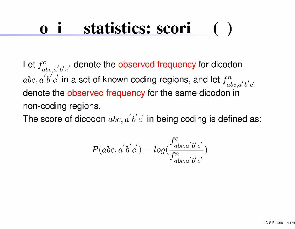
Let f ab ;a0b0 0 denote the observed frequen y for di odonab ; a0b0 0 in a set of known oding regions, and let fnab ;a0b0 0denote the observed frequen y for the same di odon innon- oding regions.The s ore of di odon ab ; a0b0 0 in being oding is de�ned as:
P (ab ; a0b0 0) = log(f ab ;a0b0 0fnab ;a0b0 0 )
LC-SIB-2006 � p.17/80
Coding statisti s: s oring (2)
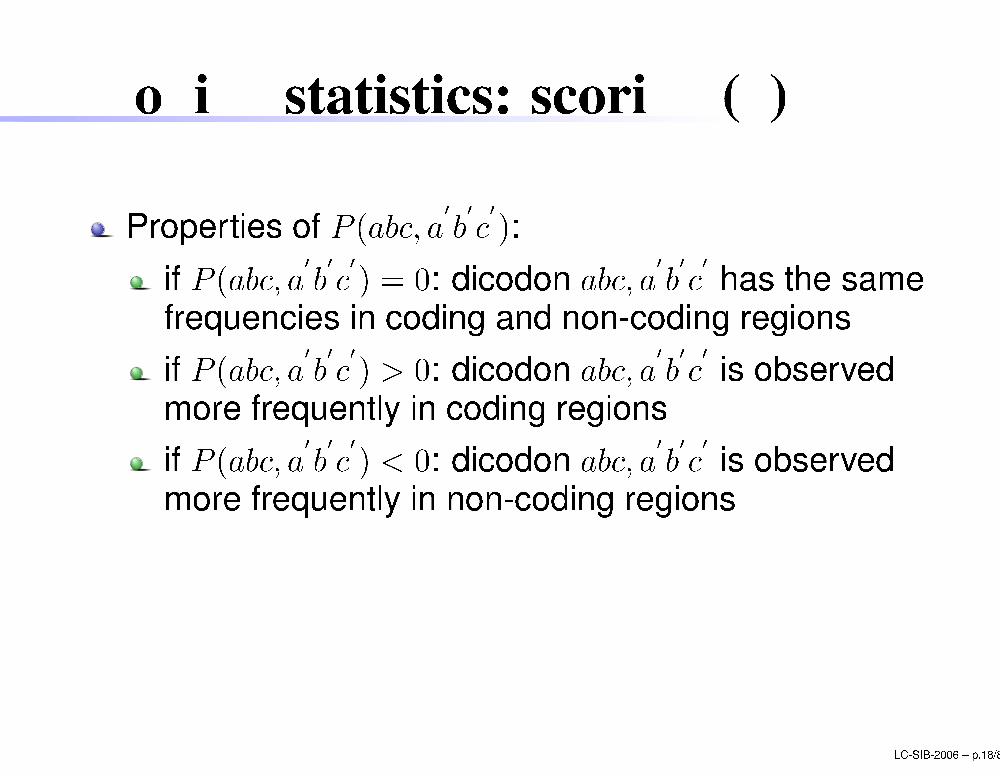
Properties of P (ab ; a0b0 0):if P (ab ; a0b0 0) = 0: di odon ab ; a0b0 0 has the samefrequen ies in oding and non- oding regionsif P (ab ; a0b0 0) > 0: di odon ab ; a0b0 0 is observedmore frequently in oding regionsif P (ab ; a0b0 0) < 0: di odon ab ; a0b0 0 is observedmore frequently in non- oding regionsLC-SIB-2006 � p.18/80
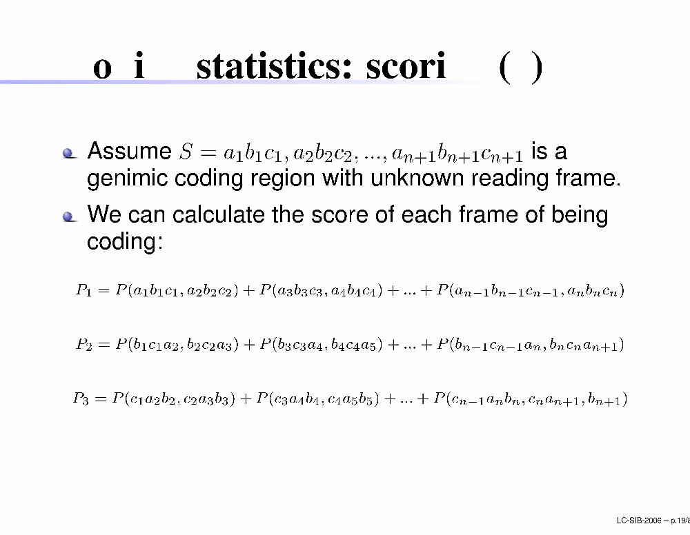
Coding statisti s: s oring (3)
Assume S = a1b1 1; a2b2 2; :::; an+1bn+1 n+1 is agenimi oding region with unknown reading frame.We an al ulate the s ore of ea h frame of being oding:P1 = P (a1b1 1; a2b2 2) + P (a3b3 3; a4b4 4) + :::+ P (an�1bn�1 n�1; anbn n)P2 = P (b1 1a2; b2 2a3) + P (b3 3a4; b4 4a5) + :::+ P (bn�1 n�1an; bn nan+1)P3 = P ( 1a2b2; 2a3b3) + P ( 3a4b4; 4a5b5) + :::+ P ( n�1anbn; nan+1; bn+1)LC-SIB-2006 � p.19/80
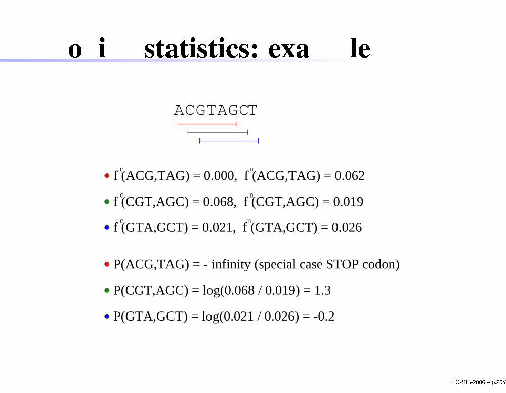
Coding statisti s: examplen
ACGTAG TC
c
c
c
f (ACG,TAG) = 0.000, f (ACG,TAG) = 0.062n
f (CGT,AGC) = 0.068, f (CGT,AGC) = 0.019n
f (GTA,GCT) = 0.021, f (GTA,GCT) = 0.026
P(CGT,AGC) = log(0.068 / 0.019) = 1.3
P(GTA,GCT) = log(0.021 / 0.026) = -0.2
P(ACG,TAG) = - infinity (special case STOP codon)
LC-SIB-2006 � p.20/80
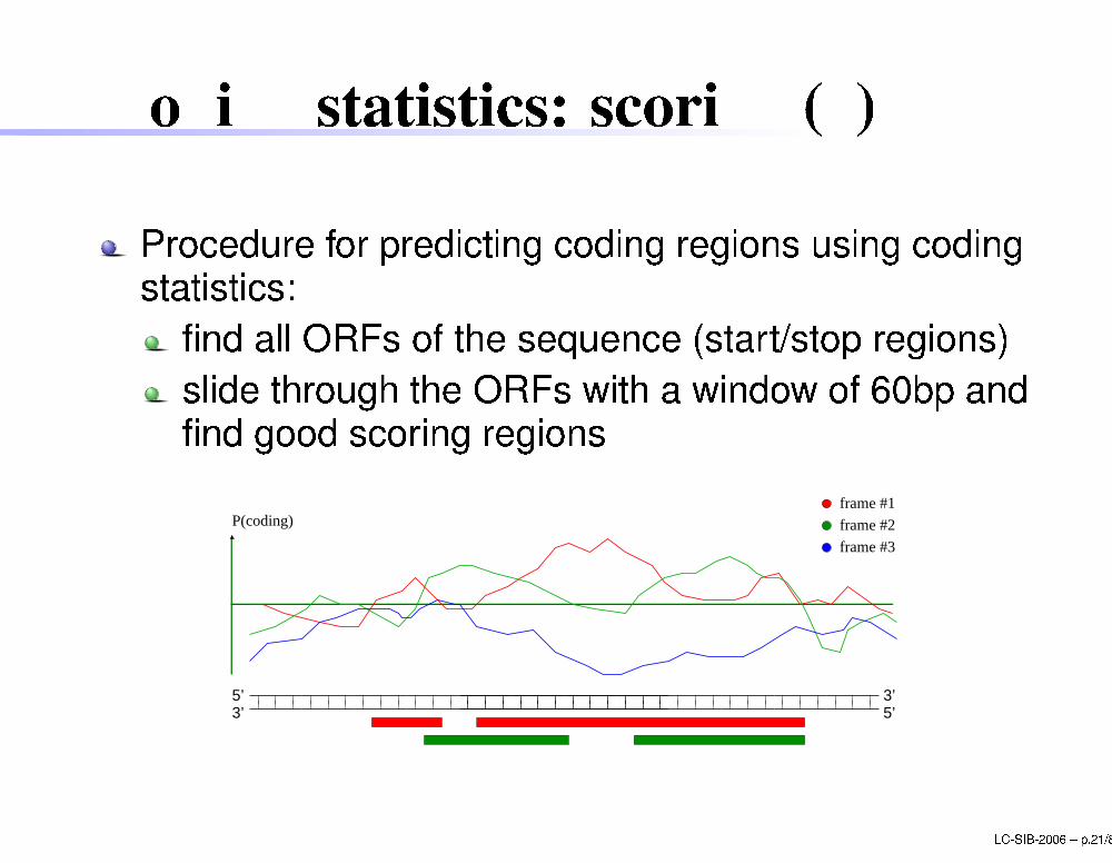
Coding statisti s: s oring (4)
Pro edure for predi ting oding regions using odingstatisti s:�nd all ORFs of the sequen e (start/stop regions)slide through the ORFs with a window of 60bp and�nd good s oring regions5’ 3’
5’
frame #3
frame #2
frame #1P(coding)
3’
LC-SIB-2006 � p.21/80
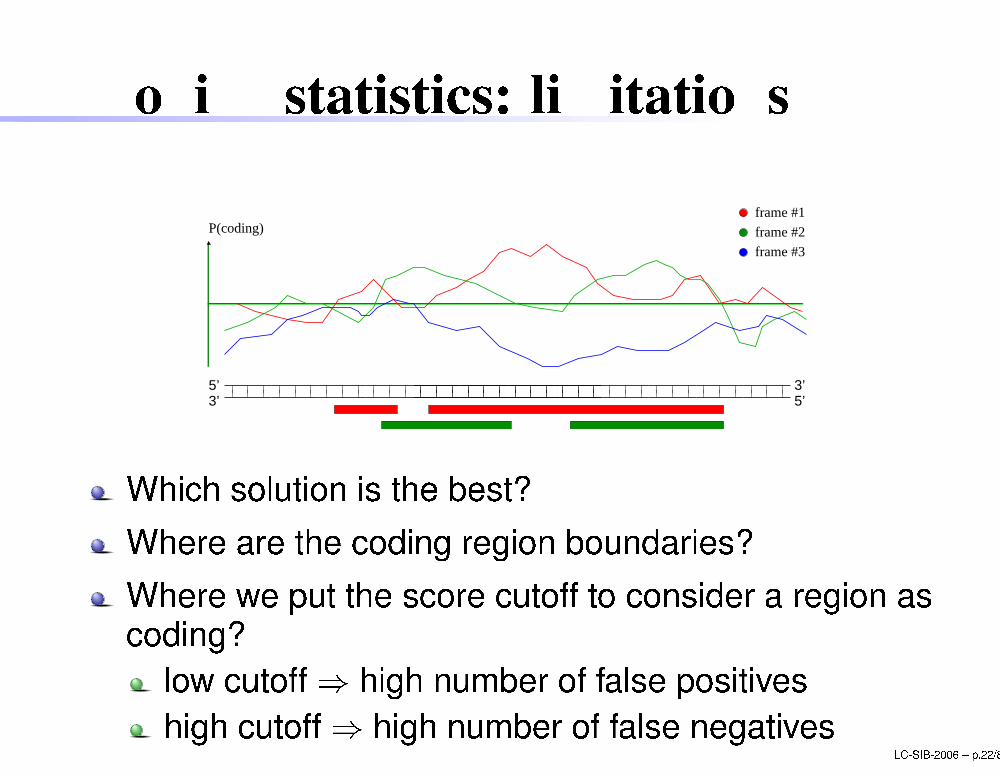
Coding statisti s: limitations5’ 3’
5’
frame #3
frame #2
frame #1P(coding)
3’
Whi h solution is the best?Where are the oding region boundaries?Where we put the s ore utoff to onsider a region as oding?low utoff) high number of false positiveshigh utoff) high number of false negatives LC-SIB-2006 � p.22/80
OutlineIntrodu tionAb initio methodsCoding statisti sSignal dete tionIntegration of signal dete tion and oding statisti sSoftwareHomology methodsPrin iple of the methodSoftwareMixing the methods: de novo methodsPerforman e evaluation LC-SIB-2006 � p.23/80
SignalsDete tion of signals in DNA sequen es helps indete ting the orre t oding regionsA number of signals an be used:promoter regionsa eptor/donor sites for spli ingintron bran hing pointspoly-adenylation...
LC-SIB-2006 � p.24/80
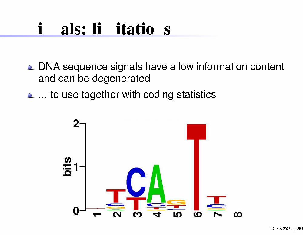
Signals: limitations
DNA sequen e signals have a low information ontentand an be degenerated... to use together with oding statisti sLC-SIB-2006 � p.25/80
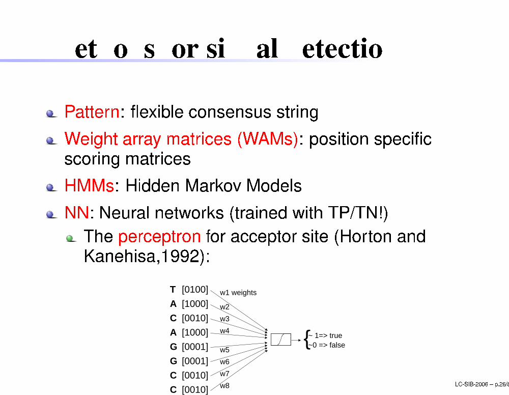
Methods for signal dete tion
Pattern: �exible onsensus stringWeight array matri es (WAMs): position spe i� s oring matri esHMMs: Hidden Markov ModelsNN: Neural networks (trained with TP/TN!)The per eptron for a eptor site (Horton andKanehisa,1992):w7
w8
w3
w4
w5
w6
{~ 1=> true
T
A
C
A
G
G
C
C
[0100]
[1000]
[0010]
[1000]
[0001]
[0001]
[0010]
[0010]
w1 weights
~0 => false
w2
1
0 LC-SIB-2006 � p.26/80
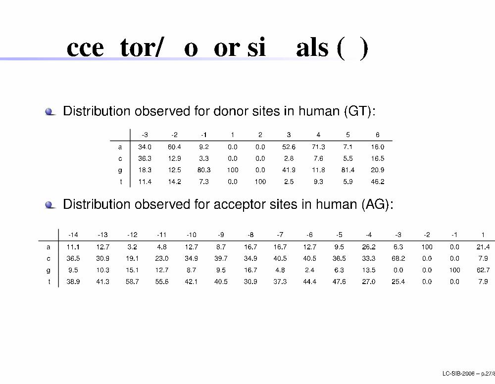
A eptor/Donor signals (1)
Distribution observed for donor sites in human (GT):-3 -2 -1 1 2 3 4 5 6a 34.0 60.4 9.2 0.0 0.0 52.6 71.3 7.1 16.0 36.3 12.9 3.3 0.0 0.0 2.8 7.6 5.5 16.5g 18.3 12.5 80.3 100 0.0 41.9 11.8 81.4 20.9t 11.4 14.2 7.3 0.0 100 2.5 9.3 5.9 46.2Distribution observed for a eptor sites in human (AG):-14 -13 -12 -11 -10 -9 -8 -7 -6 -5 -4 -3 -2 -1 1a 11.1 12.7 3.2 4.8 12.7 8.7 16.7 16.7 12.7 9.5 26.2 6.3 100 0.0 21.4 36.5 30.9 19.1 23.0 34.9 39.7 34.9 40.5 40.5 36.5 33.3 68.2 0.0 0.0 7.9g 9.5 10.3 15.1 12.7 8.7 9.5 16.7 4.8 2.4 6.3 13.5 0.0 0.0 100 62.7t 38.9 41.3 58.7 55.6 42.1 40.5 30.9 37.3 44.4 47.6 27.0 25.4 0.0 0.0 7.9LC-SIB-2006 � p.27/80
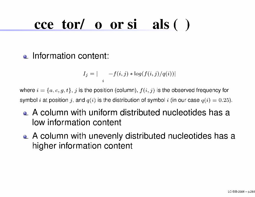
A eptor/Donor signals (2)
Information ontent:Ij = jXi �f(i; j) � log(f(i; j)=q(i))jwhere i = fa; ; g; tg, j is the position ( olumn), f(i; j) is the observed frequen y forsymbol i at position j, and q(i) is the distribution of symbol i (in our ase q(i) = 0:25).A olumn with uniform distributed nu leotides has alow information ontentA olumn with unevenly distributed nu leotides has ahigher information ontent
LC-SIB-2006 � p.28/80
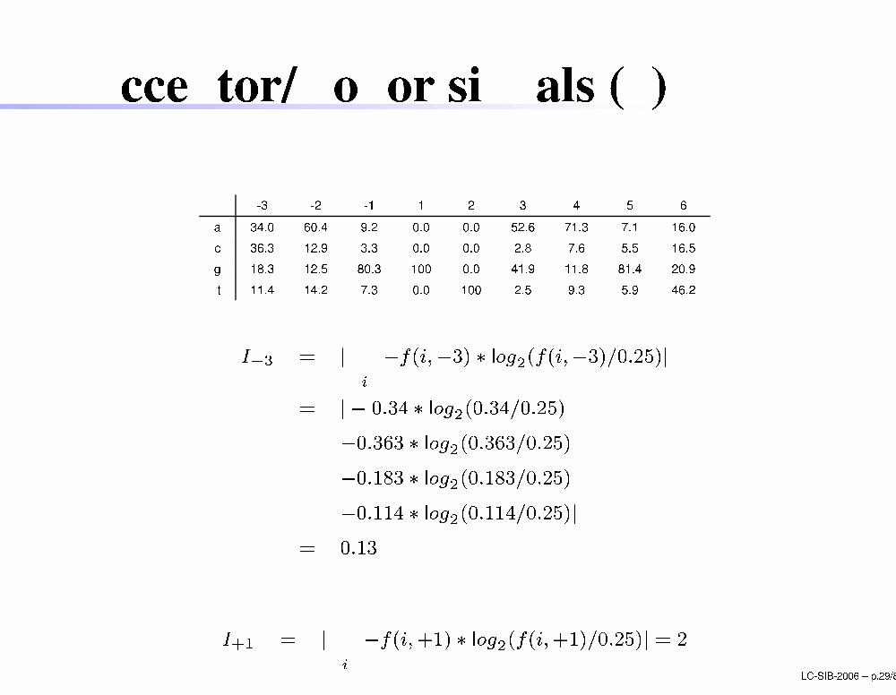
A eptor/Donor signals (3)
-3 -2 -1 1 2 3 4 5 6a 34.0 60.4 9.2 0.0 0.0 52.6 71.3 7.1 16.0 36.3 12.9 3.3 0.0 0.0 2.8 7.6 5.5 16.5g 18.3 12.5 80.3 100 0.0 41.9 11.8 81.4 20.9t 11.4 14.2 7.3 0.0 100 2.5 9.3 5.9 46.2I�3 = jXi �f(i;�3) � log2(f(i;�3)=0:25)j= j � 0:34 � log2(0:34=0:25)�0:363 � log2(0:363=0:25)�0:183 � log2(0:183=0:25)�0:114 � log2(0:114=0:25)j= 0:13I+1 = jXi �f(i;+1) � log2(f(i;+1)=0:25)j = 2 LC-SIB-2006 � p.29/80
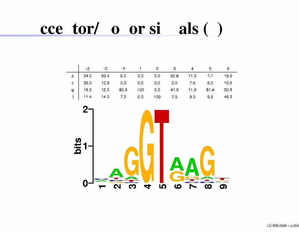
A eptor/Donor signals (4)
-3 -2 -1 1 2 3 4 5 6a 34.0 60.4 9.2 0.0 0.0 52.6 71.3 7.1 16.0 36.3 12.9 3.3 0.0 0.0 2.8 7.6 5.5 16.5g 18.3 12.5 80.3 100 0.0 41.9 11.8 81.4 20.9t 11.4 14.2 7.3 0.0 100 2.5 9.3 5.9 46.2LC-SIB-2006 � p.30/80
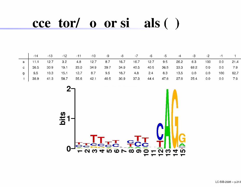
A eptor/Donor signals (5)
-14 -13 -12 -11 -10 -9 -8 -7 -6 -5 -4 -3 -2 -1 1a 11.1 12.7 3.2 4.8 12.7 8.7 16.7 16.7 12.7 9.5 26.2 6.3 100 0.0 21.4 36.5 30.9 19.1 23.0 34.9 39.7 34.9 40.5 40.5 36.5 33.3 68.2 0.0 0.0 7.9g 9.5 10.3 15.1 12.7 8.7 9.5 16.7 4.8 2.4 6.3 13.5 0.0 0.0 100 62.7t 38.9 41.3 58.7 55.6 42.1 40.5 30.9 37.3 44.4 47.6 27.0 25.4 0.0 0.0 7.9LC-SIB-2006 � p.31/80
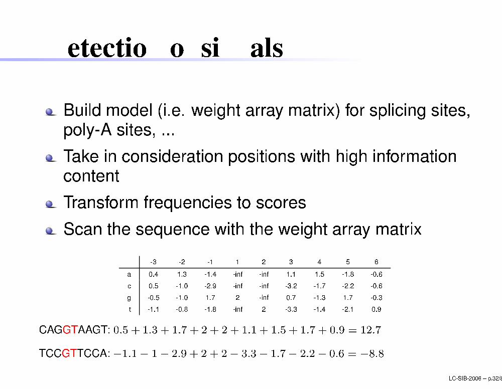
Dete tion of signals
Build model (i.e. weight array matrix) for spli ing sites,poly-A sites, ...Take in onsideration positions with high information ontentTransform frequen ies to s oresS an the sequen e with the weight array matrix-3 -2 -1 1 2 3 4 5 6a 0.4 1.3 -1.4 -inf -inf 1.1 1.5 -1.8 -0.6 0.5 -1.0 -2.9 -inf -inf -3.2 -1.7 -2.2 -0.6g -0.5 -1.0 1.7 2 -inf 0.7 -1.3 1.7 -0.3t -1.1 -0.8 -1.8 -inf 2 -3.3 -1.4 -2.1 0.9CAGGTAAGT: 0:5 + 1:3 + 1:7 + 2 + 2 + 1:1 + 1:5 + 1:7 + 0:9 = 12:7TCCGTTCCA: �1:1� 1� 2:9 + 2 + 2� 3:3� 1:7� 2:2� 0:6 = �8:8 LC-SIB-2006 � p.32/80
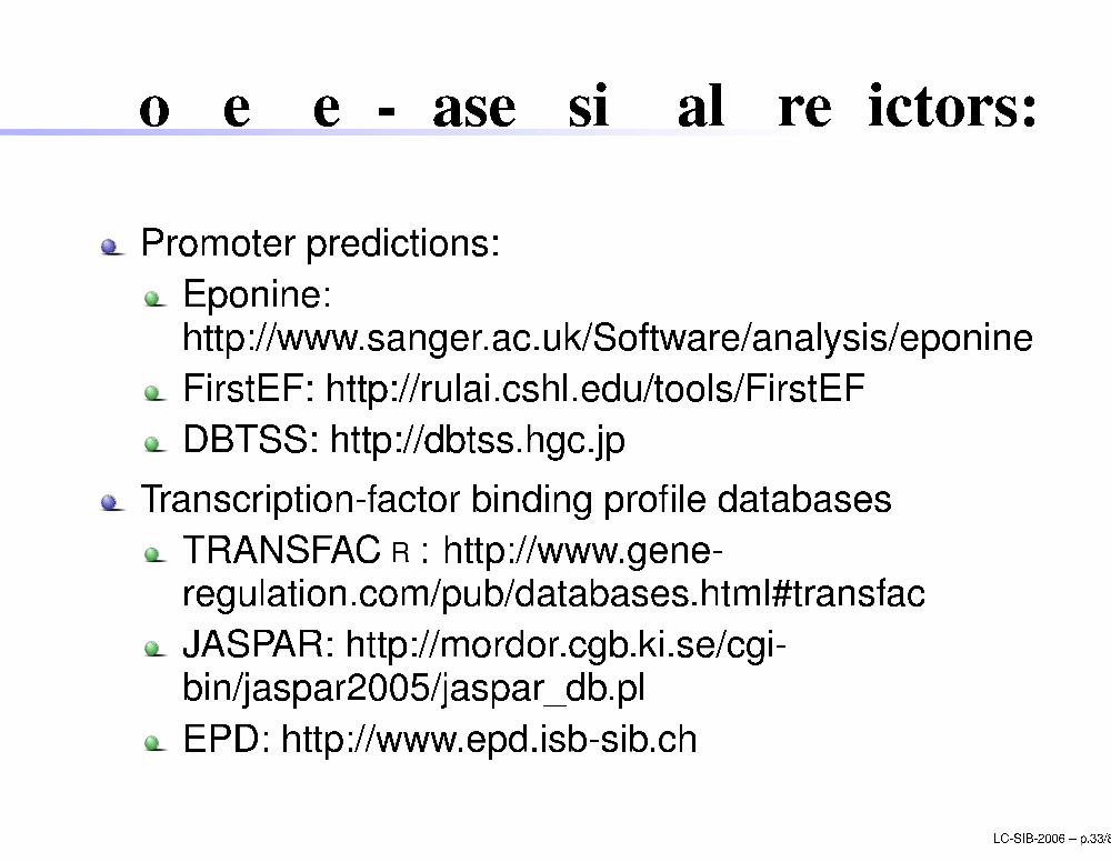
Some web-based signal predi tors:1
Promoter predi tions:Eponine:http://www.sanger.a .uk/Software/analysis/eponineFirstEF: http://rulai. shl.edu/tools/FirstEFDBTSS: http://dbtss.hg .jpTrans ription-fa tor binding pro�le databasesTRANSFAC R : http://www.gene-regulation. om/pub/databases.html#transfa JASPAR: http://mordor. gb.ki.se/ gi-bin/jaspar2005/jaspar_db.plEPD: http://www.epd.isb-sib. h
LC-SIB-2006 � p.33/80
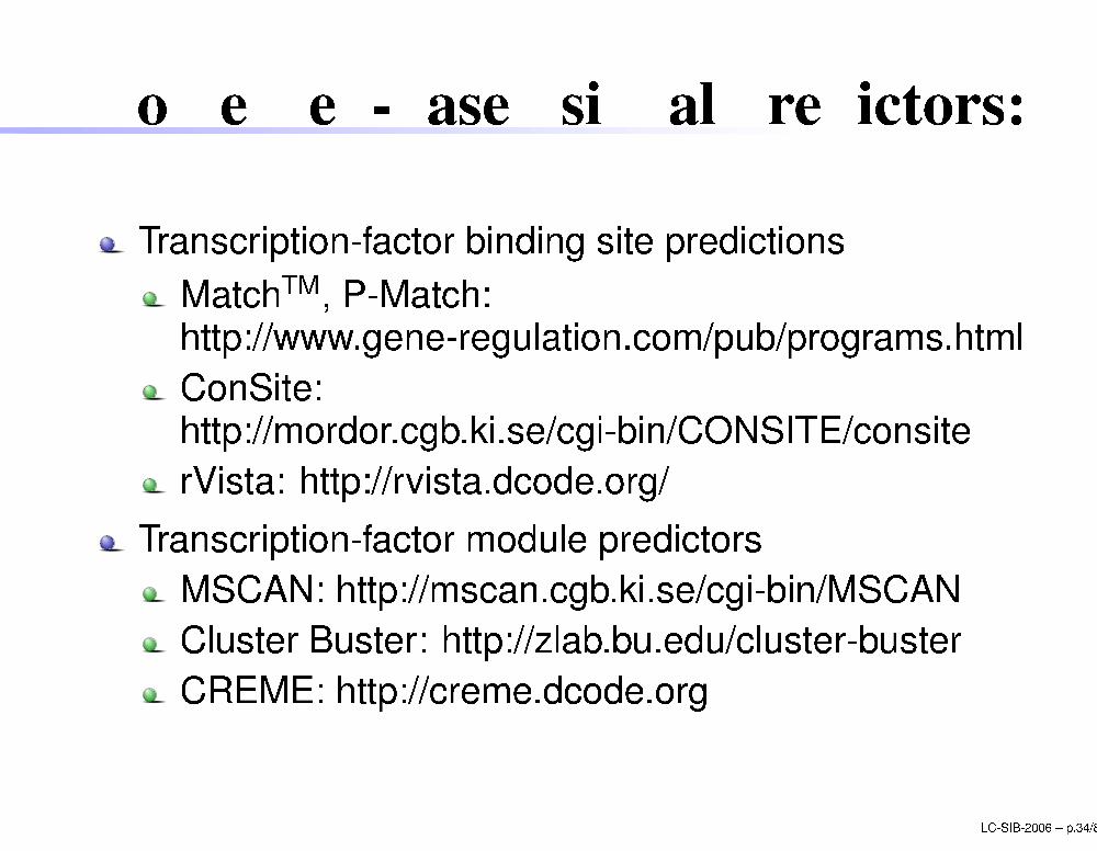
Some web-based signal predi tors:2
Trans ription-fa tor binding site predi tionsMat hTM, P-Mat h:http://www.gene-regulation. om/pub/programs.htmlConSite:http://mordor. gb.ki.se/ gi-bin/CONSITE/ onsiterVista: http://rvista.d ode.org/Trans ription-fa tor module predi torsMSCAN: http://ms an. gb.ki.se/ gi-bin/MSCANCluster Buster: http://zlab.bu.edu/ luster-busterCREME: http:// reme.d ode.org
LC-SIB-2006 � p.34/80
OutlineIntrodu tionAb initio methodsCoding statisti sSignal dete tionIntegration of signal dete tion and oding statisti sSoftwareHomology methodsPrin iple of the methodSoftwareMixing the methods: de novo methodsPerforman e evaluation LC-SIB-2006 � p.35/80
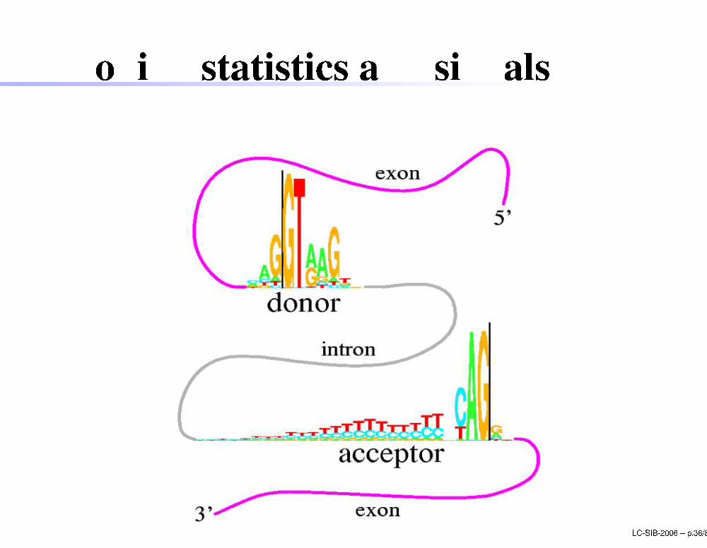
Coding statisti s and signalsLC-SIB-2006 � p.36/80
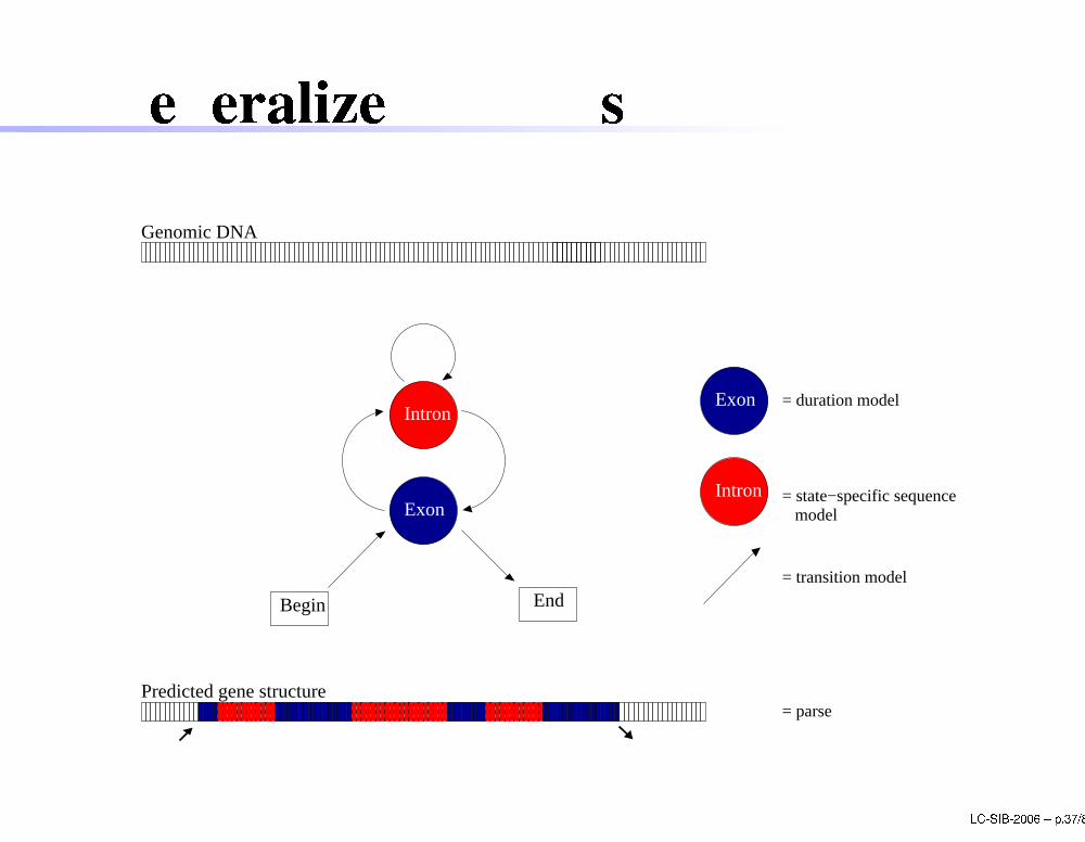
Generalized HMMsExon
Intron
Begin End
Exon
Intron
Genomic DNA
Predicted gene structure
= state−specific sequence model
= parse
= duration model
= transition model
LC-SIB-2006 � p.37/80
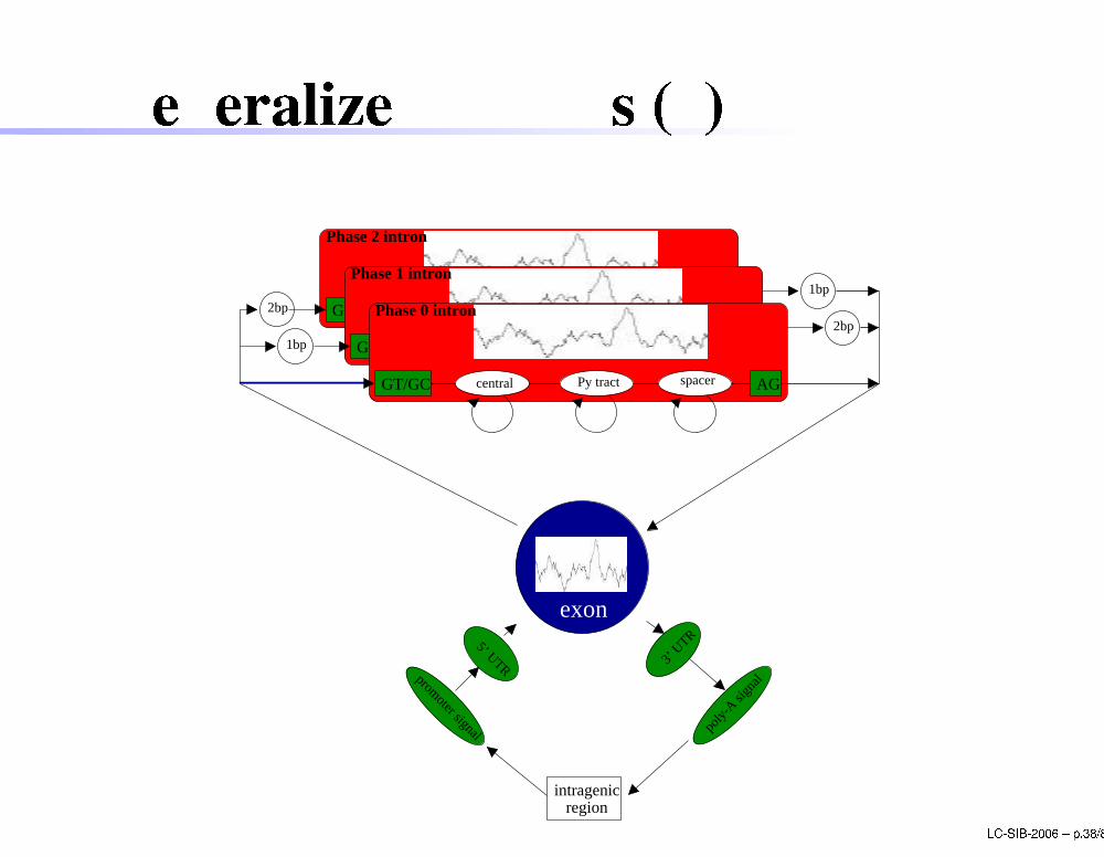
Generalized HMMs (2)1bp
1bp
2bp2bp
Phase 2 intron
GT/GC AGcentral spacerPy tract
spacerPy tract
Phase 1 intron
GT/GC AGcentral
5’ UTR 3’ U
TR
promoter signal poly-
A sign
al
intragenic region
exon
central
Phase 0 intron
Py tract spacer AGGT/GC
LC-SIB-2006 � p.38/80
Example: GENSCAN modelReverse strandForward strand
−
−
−
− −
−
− −
−
−
E2
++
E0
+
E1
I2
+
I1
+
I0
+
E term
+
E init
+
E single
++
5’ UTR
3’ UTR
+
Prom
+
PolyA
+
Prom
PolyA
E single
5’ UTR
3’ UTR
E term
E init I0
I1
I2 E2
E1
E0−
Intergenic
−
−
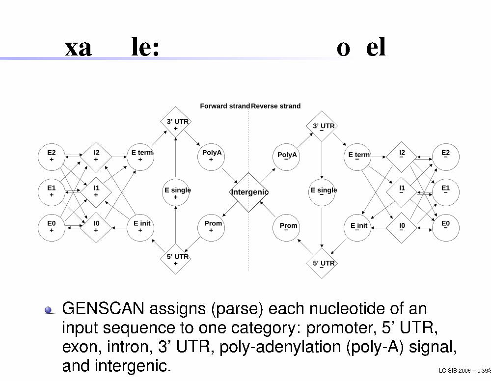
GENSCAN assigns (parse) ea h nu leotide of aninput sequen e to one ategory: promoter, 5' UTR,exon, intron, 3' UTR, poly-adenylation (poly-A) signal,and intergeni . LC-SIB-2006 � p.39/80
OutlineIntrodu tionAb initio methodsCoding statisti sSignal dete tionIntegration of signal dete tion and oding statisti sSoftwareHomology methodsPrin iple of the methodSoftwareMixing the methods: de novo methodsPerforman e evaluation LC-SIB-2006 � p.40/80
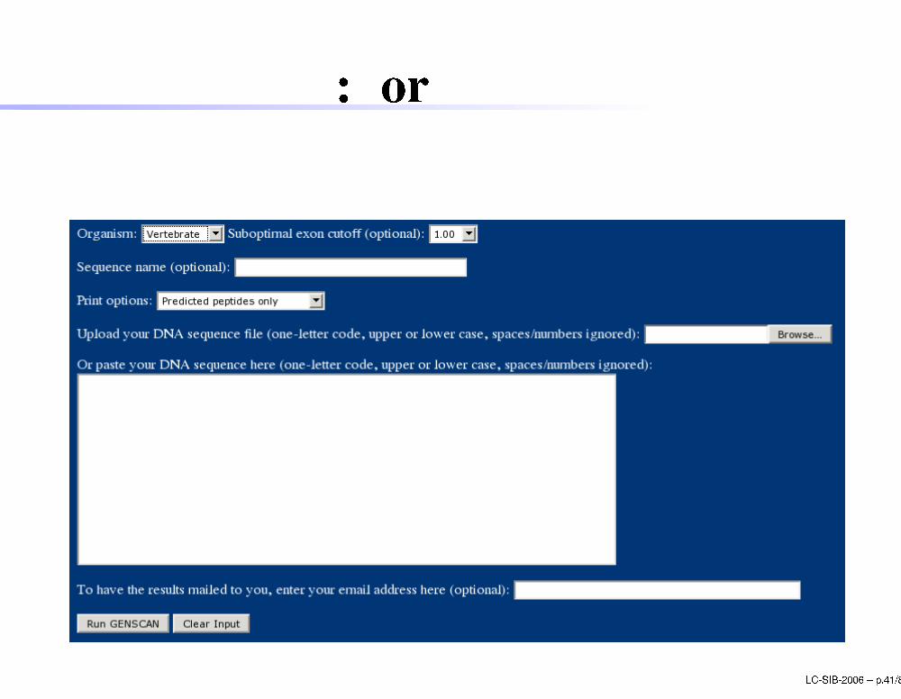
GENSCAN: form
LC-SIB-2006 � p.41/80
GENSCAN: output (1)
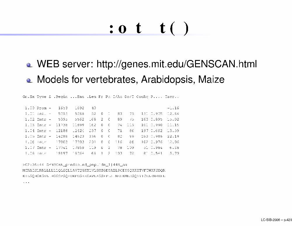
WEB server: http://genes.mit.edu/GENSCAN.htmlModels for vertebrates, Arabidopsis, MaizeGn.Ex Type S .Begin ...End .Len Fr Ph I/A Do/T CodRg P.... Ts r..----- ---- - ------ ------ ---- -- -- ---- ---- ----- ----- ------1.00 Prom + 1653 1692 40 -1.161.01 Init + 5215 5266 52 0 1 83 75 151 0.925 12.641.02 Intr + 5395 5562 168 2 0 89 75 163 0.895 15.021.03 Intr + 11738 11899 162 0 0 74 113 101 0.990 11.151.04 Intr + 12188 12424 237 0 0 71 86 197 0.662 15.391.05 Intr + 14288 14623 336 0 0 82 98 263 0.986 22.191.06 Intr + 17003 17203 201 0 0 116 86 102 0.976 12.061.07 Intr + 17741 17859 119 0 2 78 109 51 0.984 6.381.08 Intr + 18197 18264 68 1 2 103 72 81 0.541 5.70>02:36:44|GENSCAN_predi ted_peptide_1|448_aaMCRAISLRRLLLLLLQLSQLLAVTQGKTLVLGKEGESAELPCESSQKKITVFTWKFSDQRKILGQHGKGVLIRGGSPSQFDRFDSKKGAWEKGSFPLIINKLKMEDSQTYICELENRKEE...
LC-SIB-2006 � p.42/80
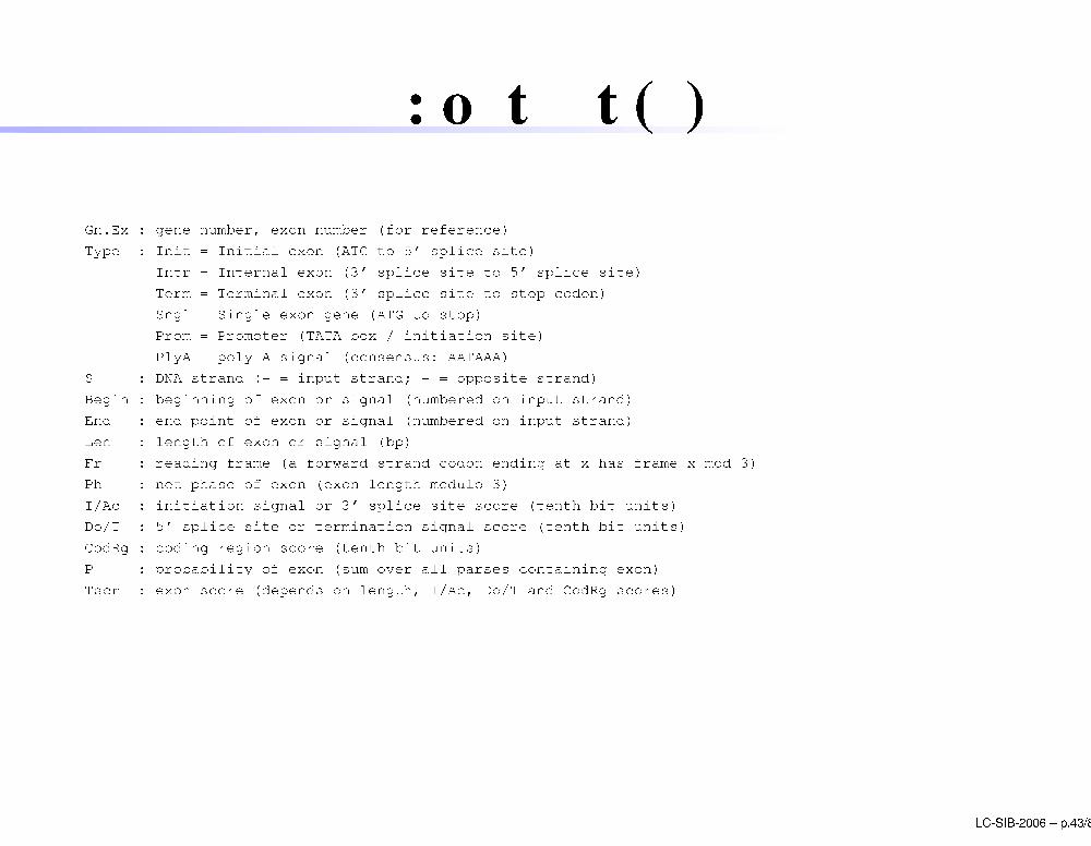
GENSCAN: output (1)
Gn.Ex : gene number, exon number (for referen e)Type : Init = Initial exon (ATG to 5' spli e site)Intr = Internal exon (3' spli e site to 5' spli e site)Term = Terminal exon (3' spli e site to stop odon)Sngl = Single-exon gene (ATG to stop)Prom = Promoter (TATA box / initiation site)PlyA = poly-A signal ( onsensus: AATAAA)S : DNA strand (+ = input strand; - = opposite strand)Begin : beginning of exon or signal (numbered on input strand)End : end point of exon or signal (numbered on input strand)Len : length of exon or signal (bp)Fr : reading frame (a forward strand odon ending at x has frame x mod 3)Ph : net phase of exon (exon length modulo 3)I/A : initiation signal or 3' spli e site s ore (tenth bit units)Do/T : 5' spli e site or termination signal s ore (tenth bit units)CodRg : oding region s ore (tenth bit units)P : probability of exon (sum over all parses ontaining exon)Ts r : exon s ore (depends on length, I/A , Do/T and CodRg s ores)
LC-SIB-2006 � p.43/80
HMMgene
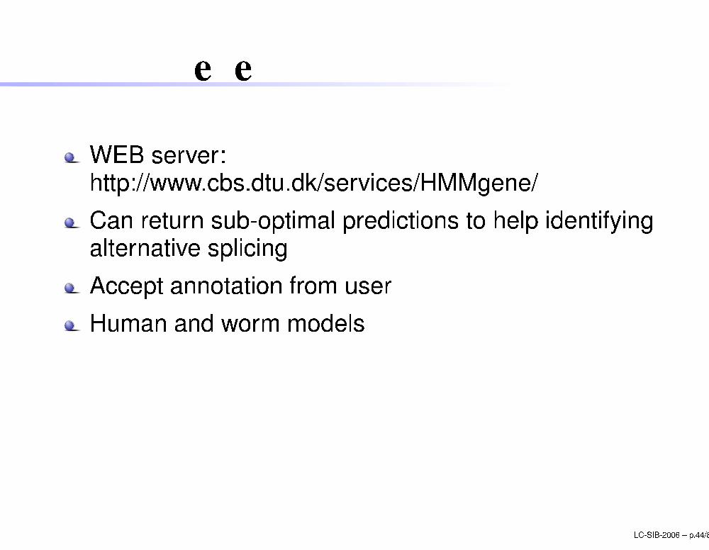
WEB server:http://www. bs.dtu.dk/servi es/HMMgene/Can return sub-optimal predi tions to help identifyingalternative spli ingA ept annotation from userHuman and worm models
LC-SIB-2006 � p.44/80
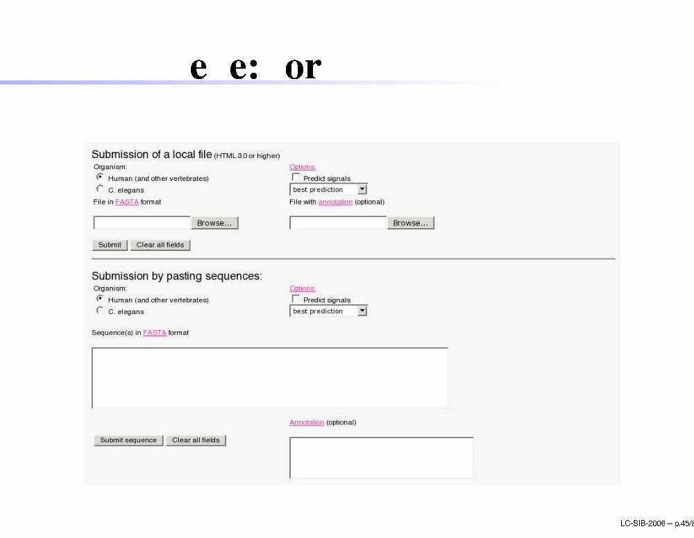
HMMgene: form
LC-SIB-2006 � p.45/80
HMMgene: output
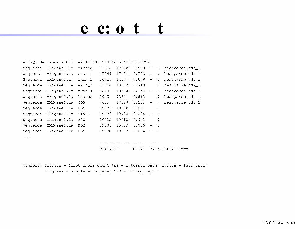
# SEQ: Sequen e 20000 (-) A:5406 C:4748 G:4754 T:5092Sequen e HMMgene1.1a firstex 17618 17828 0.578 - 1 bestparse: ds_1Sequen e HMMgene1.1a exon_1 17049 17101 0.560 - 0 bestparse: ds_1Sequen e HMMgene1.1a exon_2 14517 14607 0.659 - 1 bestparse: ds_1Sequen e HMMgene1.1a exon_3 13918 13973 0.718 - 0 bestparse: ds_1Sequen e HMMgene1.1a exon_4 12441 12508 0.751 - 2 bestparse: ds_1Sequen e HMMgene1.1a lastex 7045 7222 0.893 - 0 bestparse: ds_1Sequen e HMMgene1.1a CDS 7045 17828 0.180 - . bestparse: ds_1Sequen e HMMgene1.1a DON 19837 19838 0.001 - 1Sequen e HMMgene1.1a START 19732 19734 0.024 - .Sequen e HMMgene1.1a ACC 19712 19713 0.001 - 0Sequen e HMMgene1.1a DON 19688 19689 0.006 - 1Sequen e HMMgene1.1a DON 19686 19687 0.004 - 0... ------------ ----- ----position prob strand and frameSymbols: firstex = first exon; exon\_$n$ = internal exon; lastex = last exon;singleex = single exon gene; CDS = oding region
LC-SIB-2006 � p.46/80
GRAILexp
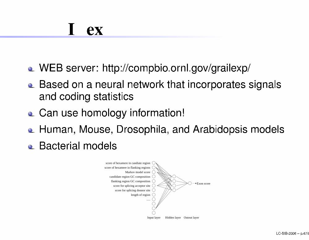
WEB server: http:// ompbio.ornl.gov/grailexp/Based on a neural network that in orporates signalsand oding statisti sCan use homology information!Human, Mouse, Drosophila, and Arabidopsis modelsBa terial modelsExon score
candidate region GC composition
score of hexamere in candiate region
score of hexamere in flanking regions
Markov model score
flanking region GC composition
score for splicing acceptor site
score for splicing donnor site
.....
length of region
Input layer Hidden layer Outout layer LC-SIB-2006 � p.47/80
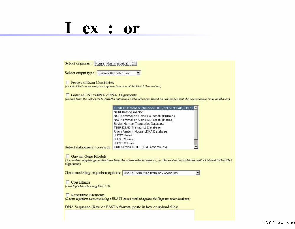
GRAILexp: form
LC-SIB-2006 � p.48/80
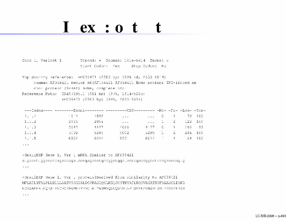
GRAILexp: output
Gene 1, Variant 1 Strand: + Bounds: 1814-6614 Exons: 5Start Codon: Yes Stop Codon: NoTop-S oring Referen e: AF038421 (2560 bp) (99% id, 2833-6614)>human|AF038421|baylor_ht|AF038421|AF038421 Homo sapiens GPI-linked an hor protein (GFRA1) mRNA, omplete dsReferen e Path: CA487395.1 (881 bp) (97%, 1814-5295)AF038421 (2560 bp) (99%, 2833-6614)---Index---- --------Exons-------- ---------CDS--------- -Ph- -Fr- -Len- -S r-1.1.1 1814 1892 ... ... 0 1 79 1001.1.2 2833 2954 ... ... 1 2 122 1001.1.3 3842 4127 4088 4127 0 1 286 991.1.4 5002 5295 5002 5295 1 2 294 1001.1.5 6531 6614 6531 6614 1 1 84 100...>GrailEXP Gene 1, Var 1 mRNA|Similar to AF038421atgaa ttgga at ag aaagat gag a tg gg tgg t taga ggt t ga agtg...>GrailEXP Gene 1, Var 1 protein|Derived from similarity to AF038421MFLATLYFALPLLDLLLSAEVSGGDRLDCVKASDQCLKEQSCSTKYRTLRQCVAGKETNFSLASGLEAKDECRSAMEALKQKSLYNCRCKRGMKKEKNCLRIYWSMYQSLQGNDLLEDSPYEPVNSRLSDIFRVVPFISX... LC-SIB-2006 � p.49/80
GeneIDUses a hierar hi al sear h stru ture:(signal! exon! gene)1st: �nds signals (spli e sites, start and stop odons)2nd: from the found signals start to s ore regionsfor exon-de�ning signals and protein- odingpotential;3rd: a dynami programming algorithm is used tosear h the spa e of predi ted exons to assemblethe gene stru ture.
LC-SIB-2006 � p.50/80
GeneIDVery fast and s ale linearly with the length of thesequen e (both in time and memory)) adapted toanalyze large sequen es.Trained with a large number of organisms.WEB site: http://www1.imim.es/geneid.html
LC-SIB-2006 � p.51/80
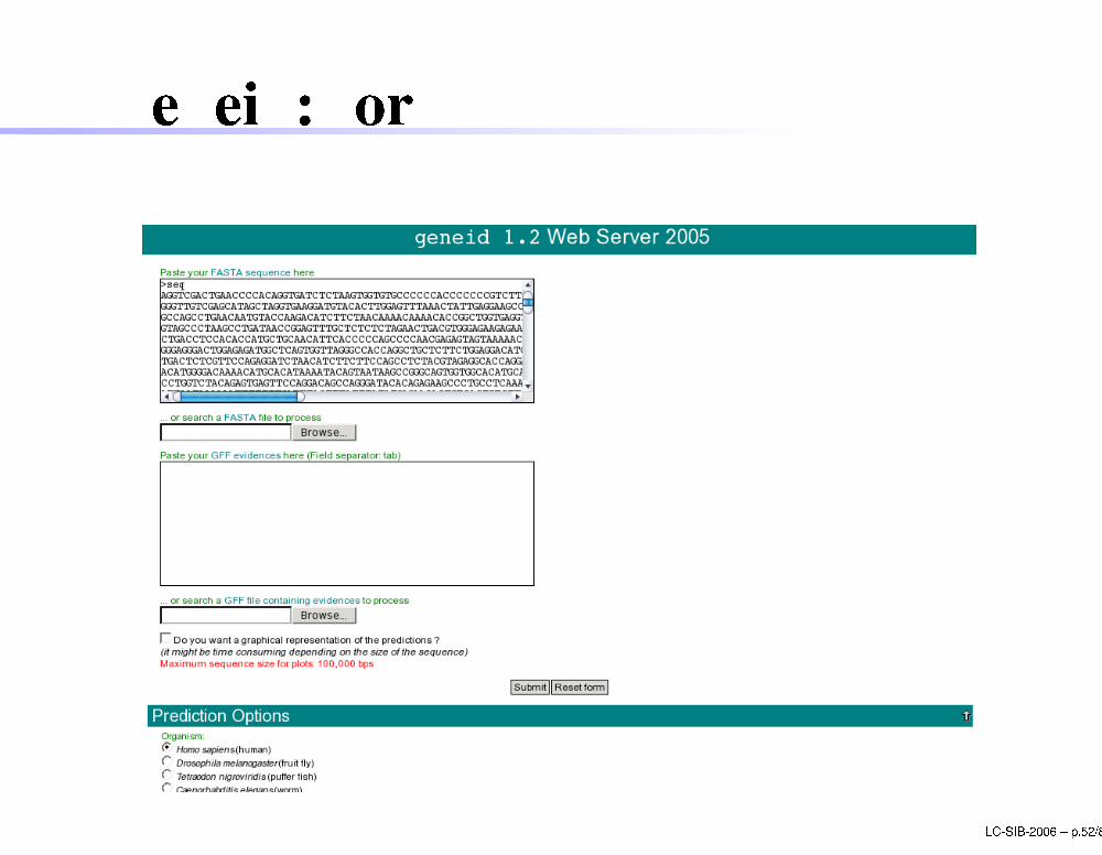
Geneid: form
LC-SIB-2006 � p.52/80
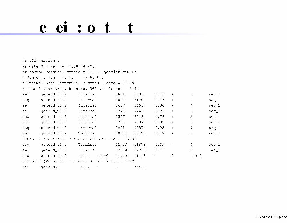
Geneid: output
## gff-version 2## date Sun Feb 26 13:38:34 2006## sour e-version: geneid v 1.2 -- geneid�imim.es# Sequen e seq - Length = 18160 bps# Optimal Gene Stru ture. 3 genes. S ore = 32.08# Gene 1 (Forward). 8 exons. 361 aa. S ore = 18.44seq geneid_v1.2 Internal 2651 2791 0.55 + 0 seq_1seq geneid_v1.2 Internal 3024 3170 2.13 + 0 seq_1seq geneid_v1.2 Internal 5427 5465 2.80 + 0 seq_1seq geneid_v1.2 Internal 7279 7441 2.35 + 0 seq_1seq geneid_v1.2 Internal 7547 7613 1.78 + 2 seq_1seq geneid_v1.2 Internal 7706 7907 0.99 + 1 seq_1seq geneid_v1.2 Internal 9071 9287 7.25 + 0 seq_1seq geneid_v1.2 Terminal 10080 10186 0.59 + 2 seq_1# Gene 2 (Reverse). 3 exons. 282 aa. S ore = 7.82seq geneid_v1.2 Terminal 11723 11878 1.09 - 0 seq_2seq geneid_v1.2 Internal 12194 12717 8.21 - 2 seq_2seq geneid_v1.2 First 14590 14755 -1.48 - 0 seq_2# Gene 3 (Forward). 1 exons. 37 aa. S ore = 5.82seq geneid78 5.82 + 0 seq_3
LC-SIB-2006 � p.53/80
OutlineIntrodu tionAb initio methodsCoding statisti sSignal dete tionIntegration of signal dete tion and oding statisti sSoftwareHomology methodsGenewiseSim4 and BLASTMixing the methods: de novo methodsPerforman e evaluation LC-SIB-2006 � p.54/80
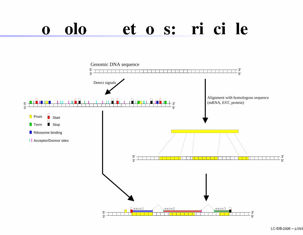
Homology methods: prin iple3’5’3’
5’Genomic DNA sequence
exon3exon2exon1
Prom
Term
Ribosome binding
Stop
Start
Acceptor/Donnor sites
5’3’5’ 3’
3’5’3’
5’
Detect signals
Alignment with homologous sequence(mRNA, EST, protein)
3’5’3’
5’ LC-SIB-2006 � p.55/80
OutlineIntrodu tionAb initio methodsCoding statisti sSignal dete tionIntegration of signal dete tion and oding statisti sSoftwareHomology methodsGenewiseSim4 and BLASTMixing the methods: de novo methodsPerforman e evaluation LC-SIB-2006 � p.56/80
GenewiseGenewise uses HMMs to align DNA sequen es toprotein sequen esPrin iple: ombine two HMMs:1. HMM to translate DNA sequen e to aa2. HMM to align translated sequen e tohomologous proteinadd transitions to deal with frame-shiftsadd intron modelGood performan es, but requires good homologoussequen es (>70%) and a lot of CPUWEB server: http://www.ebi.a .uk/Wise2/ LC-SIB-2006 � p.57/80
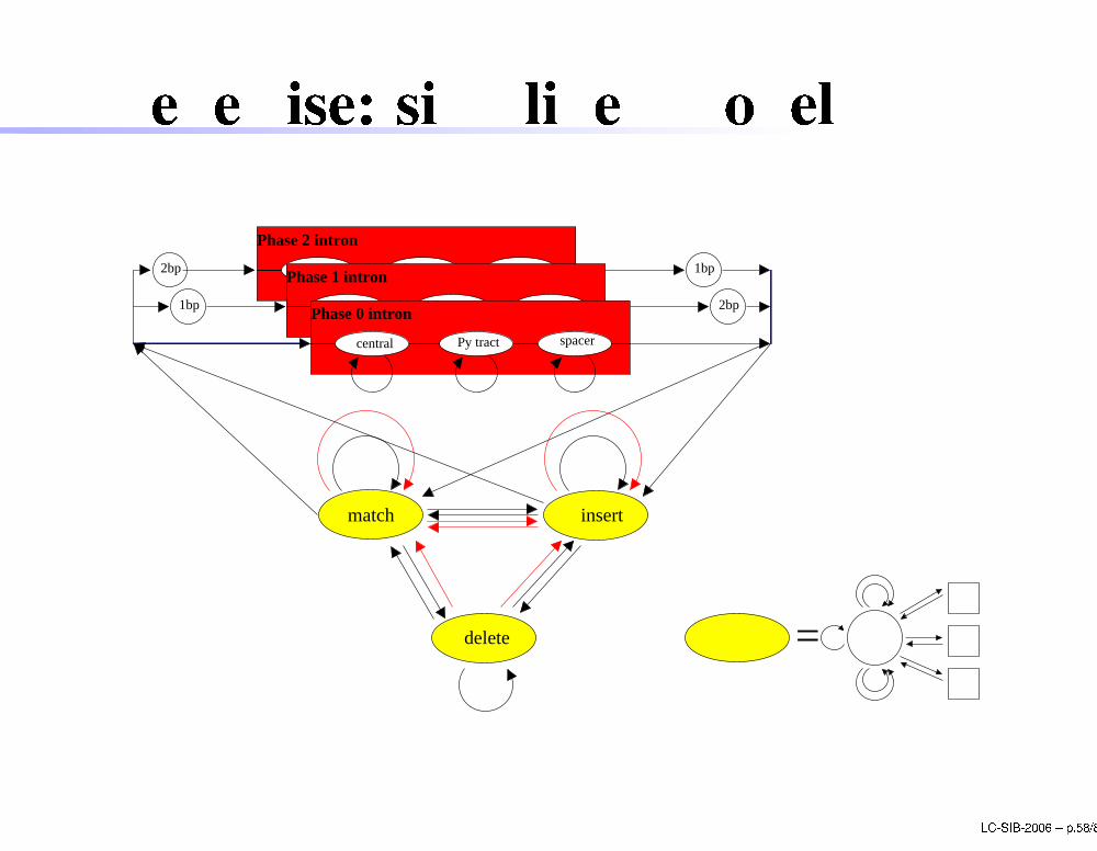
Genewise: simpli�ed modelPy tract spacercentral
Phase 2 intron
1bp2bp
1bp 2bpspacercentral Py tract
Phase 1 intron
central spacerPy tract
Phase 0 intron
=delete
insertmatch
LC-SIB-2006 � p.58/80
Genewise: form
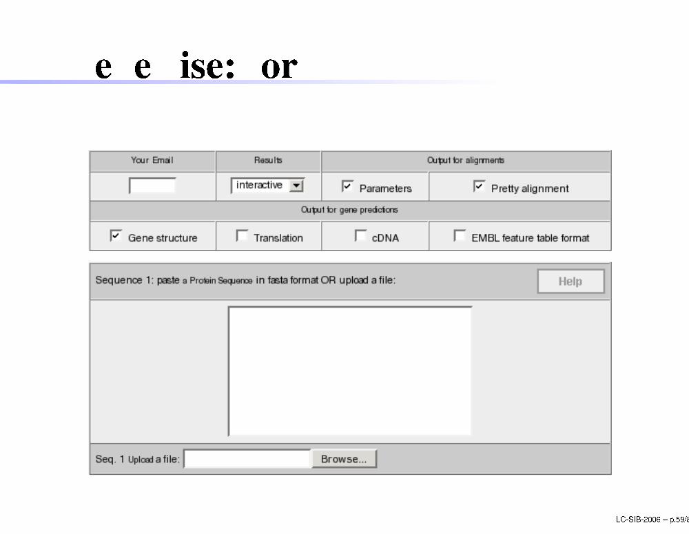
LC-SIB-2006 � p.59/80
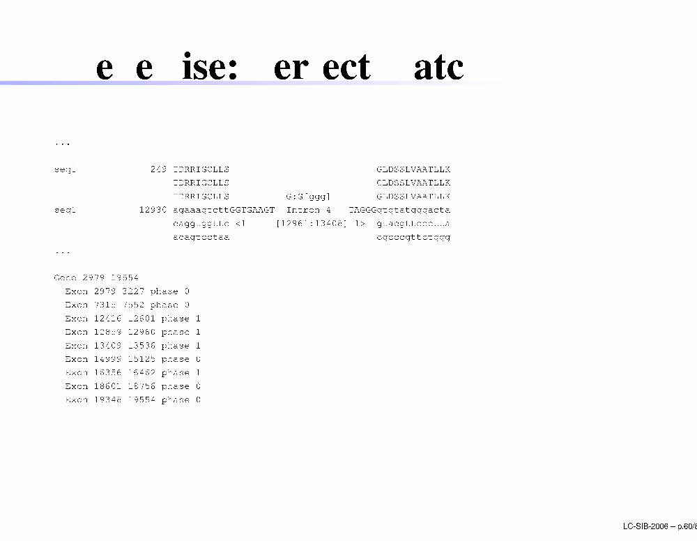
Genewise: perfe t mat h
...seq1 249 TDRRIGCLLS GLDSSLVAATLLKTDRRIGCLLS GLDSSLVAATLLKTDRRIGCLLS G:G[ggg℄ GLDSSLVAATLLKseq1 12930 agaaagt ttGGTGAAGT Intron 4 TAGGGgtgtatggga ta aggtggtt <1-----[12961:13408℄-1> gta gtt ttaa agt taa g gtt tggg...Gene 2979 19554Exon 2979 3227 phase 0Exon 7315 7552 phase 0Exon 12416 12601 phase 1Exon 12859 12960 phase 1Exon 13409 13536 phase 1Exon 14999 15125 phase 0Exon 16356 16462 phase 1Exon 18601 18756 phase 0Exon 19348 19554 phase 0
LC-SIB-2006 � p.60/80
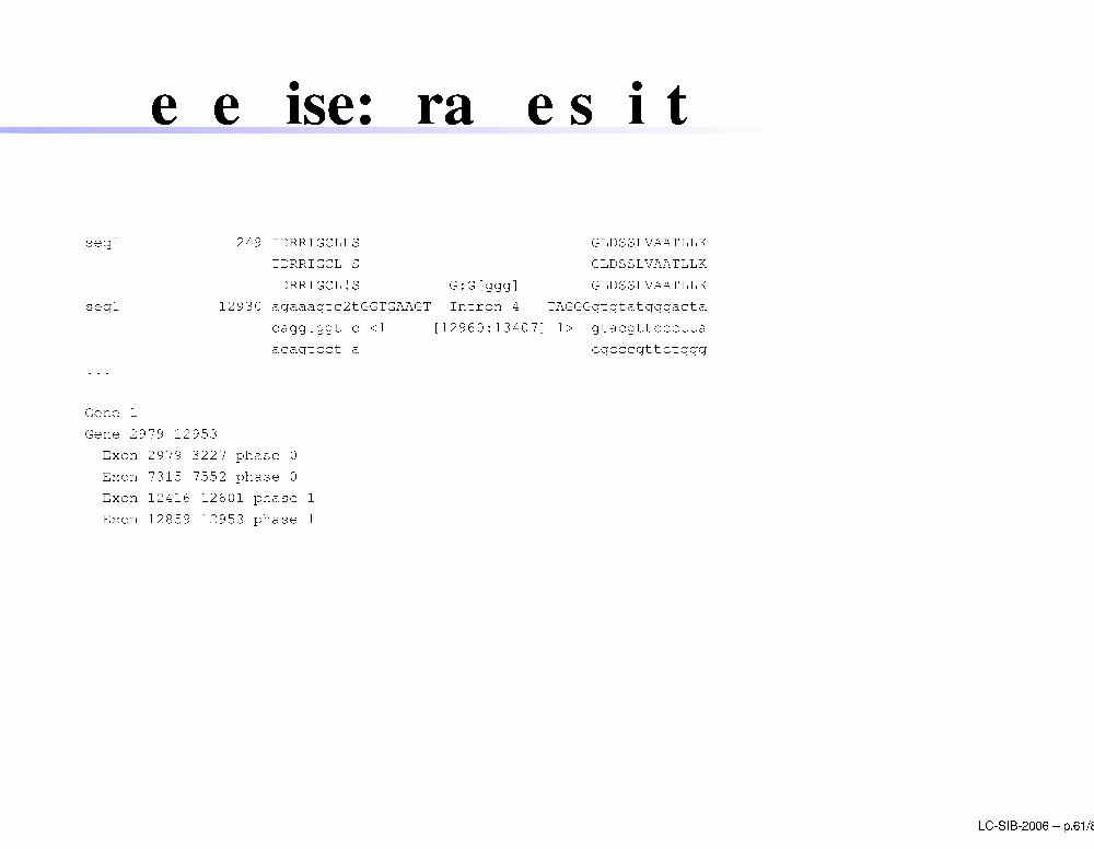
Genewise: frame shift
seq1 249 TDRRIGCLLS GLDSSLVAATLLKTDRRIGCL S GLDSSLVAATLLKTDRRIGCL!S G:G[ggg℄ GLDSSLVAATLLKseq1 12930 agaaagt 2tGGTGAAGT Intron 4 TAGGGgtgtatggga ta aggtggt <1-----[12960:13407℄-1> gta gtt ttaa agt t a g gtt tggg...Gene 1Gene 2979 12953Exon 2979 3227 phase 0Exon 7315 7552 phase 0Exon 12416 12601 phase 1Exon 12859 12953 phase 1
LC-SIB-2006 � p.61/80
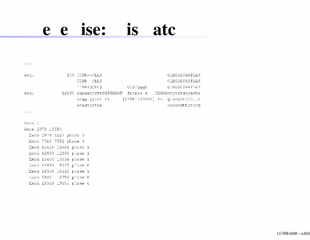
Genewise: mismat h
...seq1 249 TDRR--CLLS GLDSSLVAATLLKTDRR CLLS GLDSSLVAATLLKTDRRIGCLLS G:G[ggg℄ GLDSSLVAATLLKseq1 12930 agaaagt ttGGTGAAGT Intron 4 TAGGGgtgtatggga ta aggtggtt <1-----[12961:13408℄-1> gta gtt ttaa agt taa g gtt tggg...Gene 1Gene 2979 19554Exon 2979 3227 phase 0Exon 7315 7552 phase 0Exon 12416 12601 phase 1Exon 12859 12960 phase 1Exon 13409 13536 phase 1Exon 14999 15125 phase 0Exon 16356 16462 phase 1Exon 18601 18756 phase 0Exon 19348 19554 phase 0
LC-SIB-2006 � p.62/80
OutlineIntrodu tionAb initio methodsCoding statisti sSignal dete tionIntegration of signal dete tion and oding statisti sSoftwareHomology methodsGenewiseSim4 and BLASTMixing the methods: de novo methodsPerforman e evaluation LC-SIB-2006 � p.63/80
sim4sim4 aligns DNA to genomi sequen essim4 performs standard dynami programming, but:models spli e sitesintrons are treated as a spe ial kind of gaps withlow penaltiessim4 performs very well, but needs strong similaritybetween the sequen es
LC-SIB-2006 � p.64/80
sim4 output
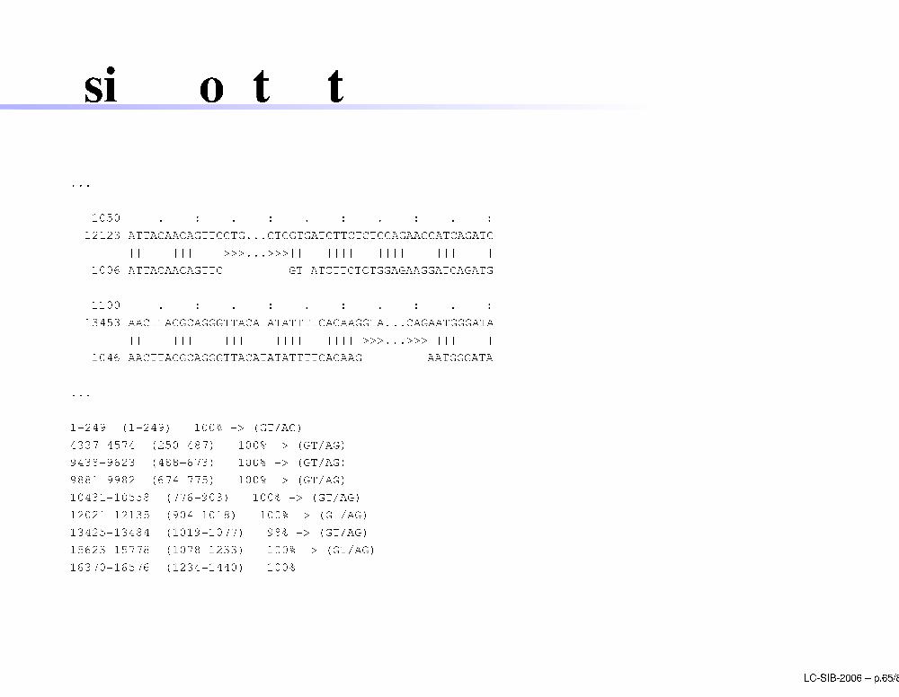
...1050 . : . : . : . : . :12123 ATTACAACAGTTCGTG...GTGGTGATCTTCTCTGGAGAAGGATCAGATG|||||||||||||>>>...>>>||-|||||||||||||||||||||||||1006 ATTACAACAGTTC GT ATCTTCTCTGGAGAAGGATCAGATG1100 . : . : . : . : . :13453 AACTTACGCAGGGTTACATATATTTTCACAAGGTA...CAGAATGGGATA||||||||||||||||||||||||||||||||>>>...>>>|||||||||1046 AACTTACGCAGGGTTACATATATTTTCACAAG AATGGGATA...1-249 (1-249) 100% -> (GT/AG)4337-4574 (250-487) 100% -> (GT/AG)9438-9623 (488-673) 100% -> (GT/AG)9881-9982 (674-775) 100% -> (GT/AG)10431-10558 (776-903) 100% -> (GT/AG)12021-12135 (904-1018) 100% -> (GT/AG)13425-13484 (1019-1077) 98% -> (GT/AG)15623-15778 (1078-1233) 100% -> (GT/AG)16370-16576 (1234-1440) 100%
LC-SIB-2006 � p.65/80
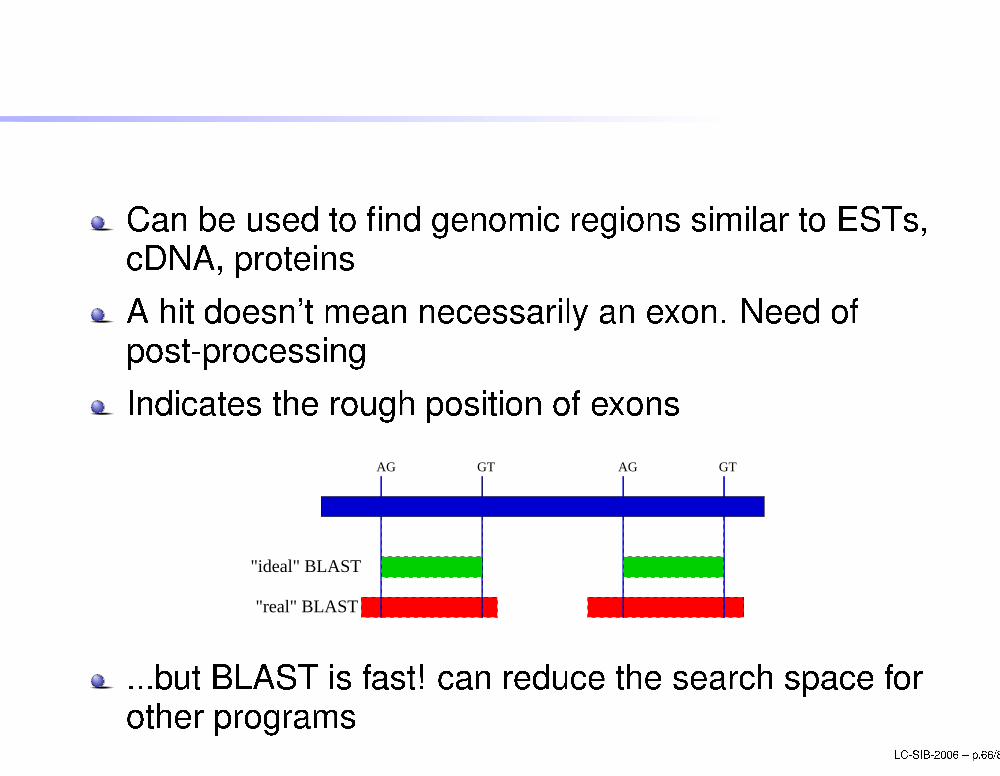
BLASTCan be used to �nd genomi regions similar to ESTs, DNA, proteinsA hit doesn't mean ne essarily an exon. Need ofpost-pro essingIndi ates the rough position of exons
"real" BLAST
"ideal" BLAST
AGGT GTAG
...but BLAST is fast! an redu e the sear h spa e forother programs LC-SIB-2006 � p.66/80
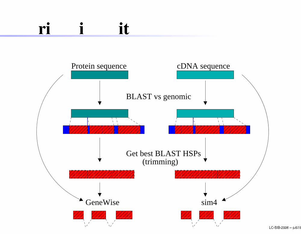
Trimming with BLAST
sim4
����������������
����������������
������������
����������������
����������������
������������
����������������
����������������
��������
������������
������������
����������������
������������
����������������
��������
������������
������������
������������
Protein sequence cDNA sequence
BLAST vs genomic
Get best BLAST HSPs(trimming)
GeneWise LC-SIB-2006 � p.67/80
OutlineIntrodu tionAb initio methodsCoding statisti sSignal dete tionIntegration of signal dete tion and oding statisti sSoftwareHomology methodsGenewiseSim4 and BLASTMixing the methods: de novo methodsPerforman e evaluation LC-SIB-2006 � p.68/80
De novo methods
Rely on the fa t that fun tional regions of a genomi sequen e, protein oding sequen es in parti ular, aremore onserved during evolution than non-fun tionalones.Use two types of information:ab initio predi tionsalignments between two or more synteni genomesequen esCurrent state-of-the-art methods for gene stru turepredi tion.
LC-SIB-2006 � p.69/80
De novo methods: Slam
Slam probabilisti model is a generalized pair hiddenMarkov model (GPHMM):GHMMs, as used in GENSCAN;pair hidden Markov models (PHMMs):emit pairs of residues) outputs in every stateare aligned pairs of DNA bases an be onsidered equivalent to theNeedleman-Wuns h alignment methodThe ombination of PHMMs with GHMMs results ingeneralized states emitting 2 sets of duration for theexons, one for ea h sequen e.
LC-SIB-2006 � p.70/80
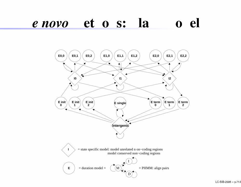
De novo methods: Slam model
E term
I
E singleE init E init E init E term E term0 01 2 1 2
E0,0 E0,1 E0,2 E1,0 E1,1 E1,2 E2,0 E2,1 E2,2
I0 I1 I2
E
Intergenic
= duration model = = PHMM: align pairsM
I
D
= state specific model: model unrelated n on−coding regions model conserved non−coding regions
LC-SIB-2006 � p.71/80
De novo methods: Twins an
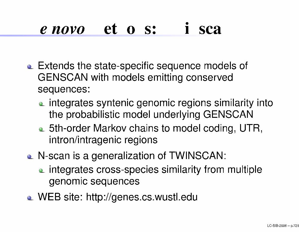
Extends the state-spe i� sequen e models ofGENSCAN with models emitting onservedsequen es:integrates synteni genomi regions similarity intothe probabilisti model underlying GENSCAN5th-order Markov hains to model oding, UTR,intron/intrageni regionsN-s an is a generalization of TWINSCAN:integrates ross-spe ies similarity from multiplegenomi sequen esWEB site: http://genes. s.wustl.edu
LC-SIB-2006 � p.72/80
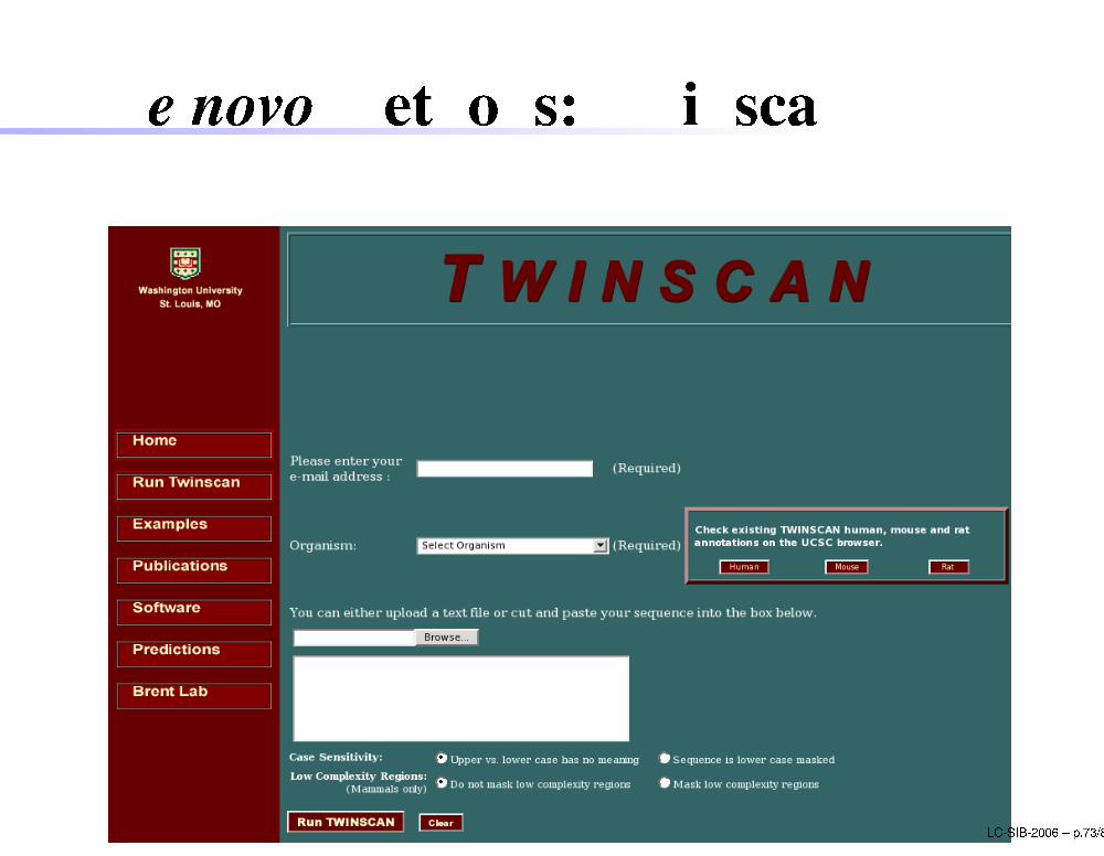
De novo methods: Twins anLC-SIB-2006 � p.73/80
De novo methods: SGP2
Predi ts gene stru ture in a target genome sequen eusing the sequen e of a se ond informant genome.Framework integrating:ab initio gene predi tion using GENEIDTBLASTX to in orporate information from theinformant genomeWEB site:http://genome.imim.es/software/sgp2/sgp2.htmlLC-SIB-2006 � p.74/80
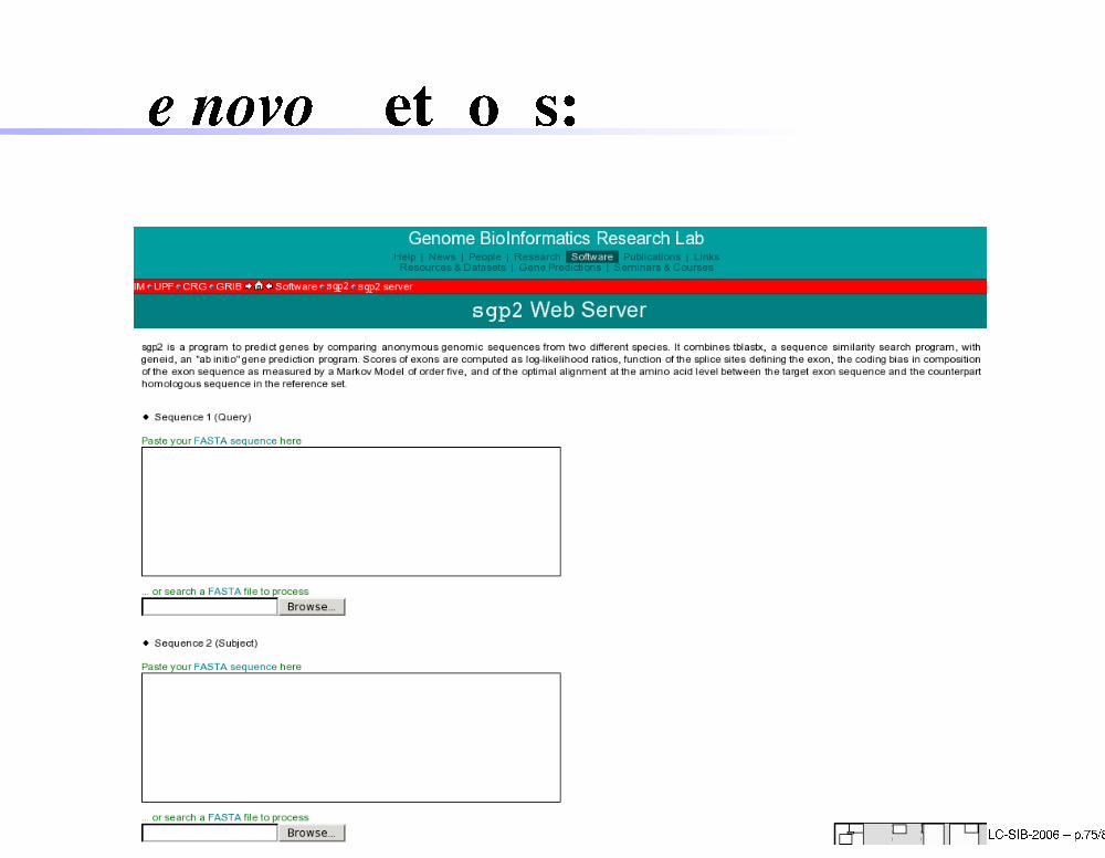
De novo methods: SGP2
LC-SIB-2006 � p.75/80
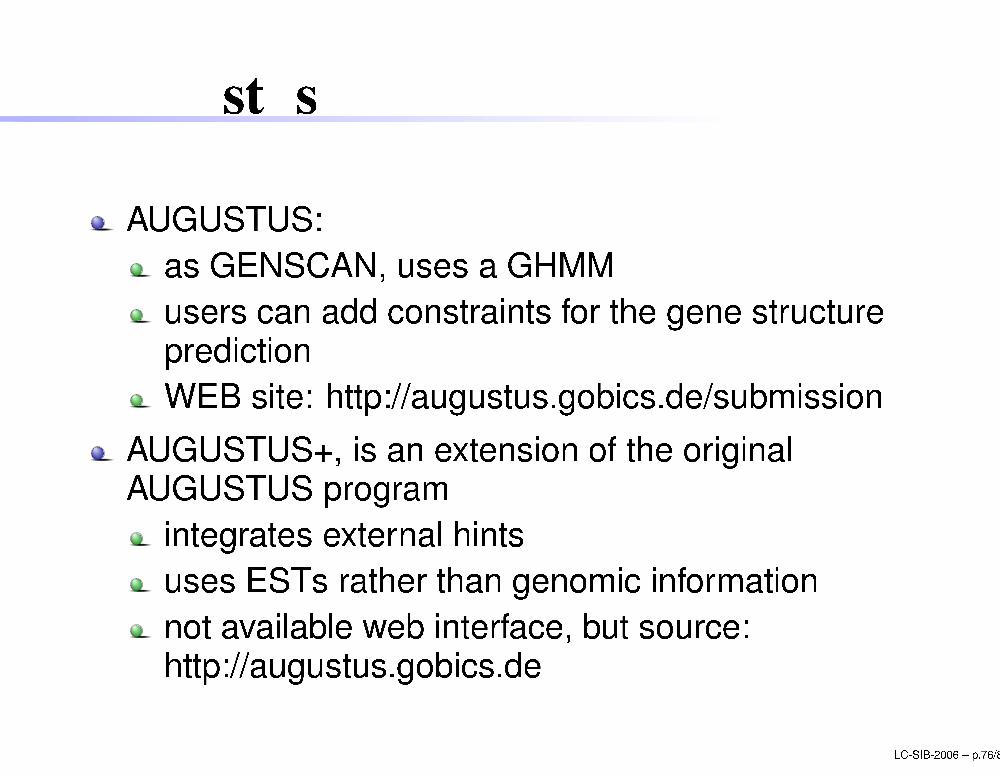
Augustus+AUGUSTUS:as GENSCAN, uses a GHMMusers an add onstraints for the gene stru turepredi tionWEB site: http://augustus.gobi s.de/submissionAUGUSTUS+, is an extension of the originalAUGUSTUS programintegrates external hintsuses ESTs rather than genomi informationnot available web interfa e, but sour e:http://augustus.gobi s.de
LC-SIB-2006 � p.76/80

De novo methods: AugustusLC-SIB-2006 � p.77/80
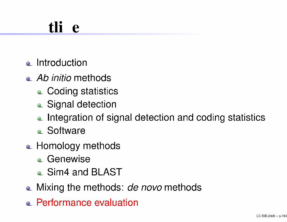
OutlineIntrodu tionAb initio methodsCoding statisti sSignal dete tionIntegration of signal dete tion and oding statisti sSoftwareHomology methodsGenewiseSim4 and BLASTMixing the methods: de novo methodsPerforman e evaluation LC-SIB-2006 � p.78/80
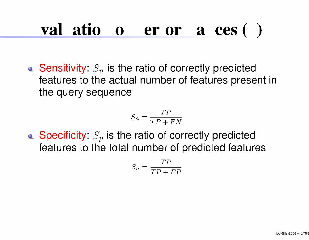
Evaluation of performan es (1)
Sensitivity: Sn is the ratio of orre tly predi tedfeatures to the a tual number of features present inthe query sequen eSn = TPTP + FNSpe i� ity: Sp is the ratio of orre tly predi tedfeatures to the total number of predi ted featuresSn = TPTP + FP
LC-SIB-2006 � p.79/80
Evaluation of performan es (2)
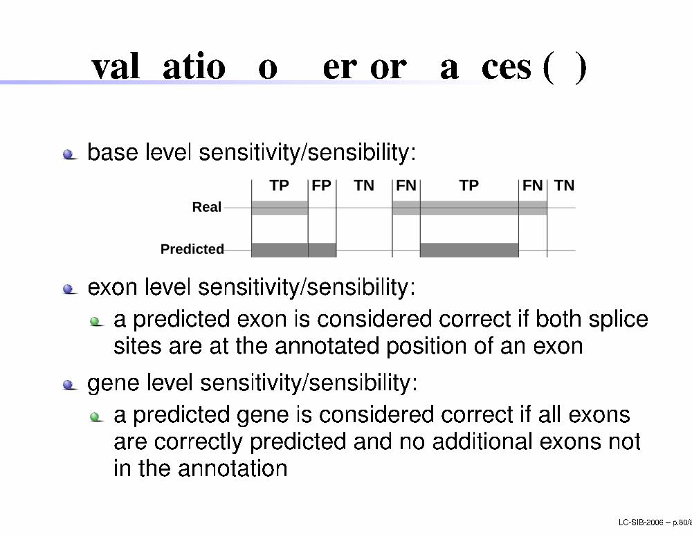
base level sensitivity/sensibility:Real
FP TNTP FN TP FN TN
Predictedexon level sensitivity/sensibility:a predi ted exon is onsidered orre t if both spli esites are at the annotated position of an exongene level sensitivity/sensibility:a predi ted gene is onsidered orre t if all exonsare orre tly predi ted and no additional exons notin the annotation LC-SIB-2006 � p.80/80
Evaluation of performan es (3)
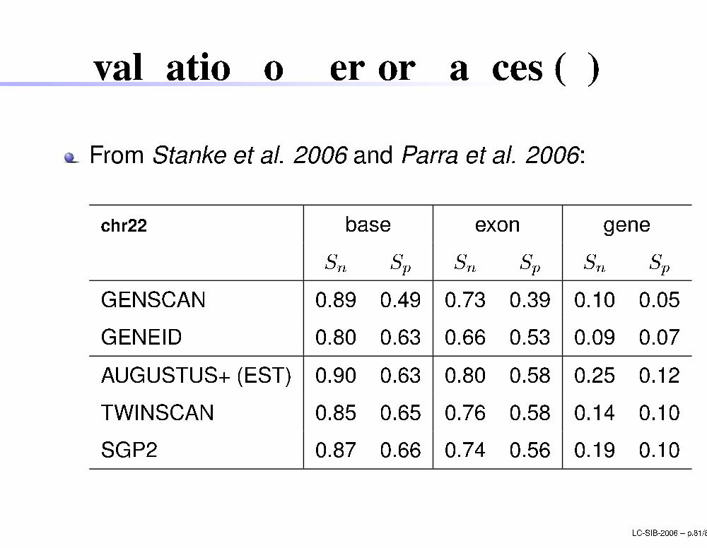
From Stanke et al. 2006 and Parra et al. 2006:
hr22 base exon geneSn Sp Sn Sp Sn SpGENSCAN 0.89 0.49 0.73 0.39 0.10 0.05GENEID 0.80 0.63 0.66 0.53 0.09 0.07AUGUSTUS+ (EST) 0.90 0.63 0.80 0.58 0.25 0.12TWINSCAN 0.85 0.65 0.76 0.58 0.14 0.10SGP2 0.87 0.66 0.74 0.56 0.19 0.10LC-SIB-2006 � p.81/80
LimitsExisting predi tors are for protein oding regionsPredi tions work �ne for "typi al" genes:�rst and last exons are dif� ult to predi tpartial gene are often missedtraining sets may be biasedatypi al genes use others grammars
LC-SIB-2006 � p.82/80

... offee!
LC-SIB-2006 � p.83/80


![a c:] 5 ooÐ L B 10.5 1 - Microsoft Word Abc Abc Abc Abc Abc Abc Abc Abc Abc Abc Abc Abc 1 - Microsoft Word Abc Abc Abc 505 7ï—L Mic SmartArt 1 - Microsoft Word Aa MS B 10.5 (Ctrl+L)](https://img.pdfslide.tips/doc/110x75/5b180d777f8b9a19258b6a1e/a-c-5-ood-l-b-105-1-microsoft-word-abc-abc-abc-abc-abc-abc-abc-abc-abc-abc.jpg)


![森・里・街・ひとがきらめく ふるさと 南丹市 : 公式ホームページ · C]^_`4a3b cc ABCª«¬IJ,-0 + C]^_`4a3b c" ABC®¬IJ,-0 + C]^_`4a3b c ABC g IJ,-0 +](https://img.pdfslide.tips/doc/110x75/60692ce44cf17621777957d3/feoefefoe-fffff.jpg)