Embed Size (px)
Citation preview

ii
Critical Process Requirements for Membrane Desalination of Agricultural Drainage in the San Joaquin Valley
DRAFT
Final Project Report Project Period: 9/01/04‐8/31/07
Interagency Agreement 4600003343
submitted to the
Agricultural Drainage Program California Department of Water Resources
3374 Sheilds Avenue Fresno, California 93726
by
Yoram Cohen1 and Brian McCool Water Technology Research Center
and Chemical and Biomolecular Engineering Department University of California, Los Angeles
Los Angeles, California 90095
Other UCLA Project Participants: Julius Glater, Anditya Rahardianto and Eric Lyster
November 15, 2007
1 Author to whom correspondence should be addressed. E‐mail: [email protected]; Phone: (310) 825‐8766;
Fax: (310) 477‐3868.

iii
TABLE OF CONTENTS
TABLE OF CONTENTS ............................................................................................................................................. III
ABSTRACT ............................................................................................................................................................. IV
1. INTRODUCTION .................................................................................................................................................. 5
2. BACKGROUND .............................................................................................................................................. 6
2.1 REVERSE OSMOSIS ........................................................................................................................................ 6
FIGURE 2‐2. CUT‐AWAY OF SPIRAL WOUND RO MEMBRANE MODULE [9]. .......................................................... 7
2.2 CONCENTRATION POLARIZATION .......................................................................................................................... 7 2.3 WATER QUALITY MEASUREMENTS ......................................................................................................................... 9 2.4 RO DESALTING RECOVERY LIMITS ....................................................................................................................... 10
3. ANALYSIS .................................................................................................................................................... 11
3.1 FIELD WATER SITE SELECTION FOR SAMPLING AND ANALYSIS ................................................................................... 11 3.2 RECOVERY LIMITS ............................................................................................................................................ 12 3.3 DIAGNOSTIC FLUX DECLINE EXPERIMENTS ............................................................................................................ 14 3.4 EQUIVALENT RECOVERY CALCULATIONS FOR DIAGNOSTIC EXPERIMENTS .................................................................... 14
4. EXPERIMENTAL ........................................................................................................................................... 15
4.1 MATERIALS & REAGENTS .................................................................................................................................. 15 4.1.1 Laboratory Work ................................................................................................................................. 15 4.1.2 Field Water Samples ........................................................................................................................... 15
4.2 APPARATUS .................................................................................................................................................... 15 4.3 DIAGNOSTIC PROCEDURE .................................................................................................................................. 17
4.3.1 Pretreatment ...................................................................................................................................... 17 4.3.2 Membrane Preparation ...................................................................................................................... 18 4.3.3 Membrane Conditioning ..................................................................................................................... 18 4.3.4 Flux Decline Run .................................................................................................................................. 18 4.3.5 System Cleaning .................................................................................................................................. 19
4.4 BIOFOULING POTENTIAL EXPERIMENTS ................................................................................................................ 19 4.4.1 Protein Assay ...................................................................................................................................... 19 4.4.2 Cultures ............................................................................................................................................... 19
5. RESULTS AND DISCUSSION ......................................................................................................................... 20
5.1 VARIABILITY OF AGRICULTURAL BRACKISH WATER QUALITY (1999–2003; 2006–2007) ............................................ 20 5.1.1 Field Water Site Selection for Sampling and Analysis ......................................................................... 20 5.1.2 Recent DWR Periodic Monitoring Data (1999–2003) ......................................................................... 27 5.1.3 Field Water Sample Data (2006–2007) .............................................................................................. 46
5.2 DIAGNOSTIC FLUX DECLINE EXPERIMENTS ............................................................................................................ 55 5.3 BIOFOULING POTENTIAL AND PARTICULATES ......................................................................................................... 68
6. CONCLUSIONS AND RECOMMENDATIONS ...................................................................................................... 69
6.1 CONCLUSIONS ............................................................................................................................................ 69 6.2 RECOMMENDATIONS ................................................................................................................................... 70
7. REFERENCES ............................................................................................................................................... 71

iv
ABSTRACT
The use of reverse osmosis (RO) desalting for treating brackish agricultural drainage (AD) water
in the San Joaquin Valley (SJV) was evaluated as a potential method for reducing the salinity of brackish
drainage discharge and thus providing for reclamation and reuse of this water source. A systematic
approach was developed using thermodynamic solubility analysis and diagnostic RO scaling experiments
in a plate‐and‐frame RO system with a commercial low‐pressure RO membrane to determine product
water recovery limits with respect to the source water chemistry. Analysis of available SJV water quality
monitoring data revealed substantial seasonal and spatial water quality variations. Water sources in a
number of locations were nearly saturated with respect to gypsum. Theoretical analysis of RO recovery
limits due to mineral scaling of sparingly soluble salts (e.g. calcite, gypsum, silica) suggested that RO
recovery would be limited to about 54% ‐ 68% (assuming the use of standard scale mitigation strategies
such as pH adjustment and antiscalant dosing). The analysis also revealed that, If limitations due to
mineral scaling could be alleviated, recovery limits imposed by osmotic pressure would range from
about 70% to 94% for 600 psi RO vessels and from about 81% to 96% for 1000 psi RO vessels. The above
analysis was supplemented by comparative diagnostic flux decline experiments using field water
samples from five different locations in the SJV. These locations were selected to be representative of
the range of water compositions throughout the San Joaquin Valley. Membrane RO desalination tests
were carried using a plate‐and‐frame module geometry. These tests were conducted such that the
average initial gypsum saturation indices at the membrane surface that ranged from 0.28 to 2.1.
Equivalent recoveries (based on estimation of concentration polarization and observed salt rejection),
for the non‐scaling diagnostic tests, were in reasonable agreement with recovery limits estimated
through thermodynamic solubility analysis. RO desalination is a feasible technology for desalting SJV
drainage water. However, given the spatial and temporal water quality in the San Joaquin Valley, a
distributed system of desalination facilities would be the most appropriate approach for field‐scale
deployment of RO desalination. Such systems would require effective feed quality monitoring along with
monitoring of membrane scaling/fouling along with effective self‐initiated scaling/fouling mitigation
technologies. Pilot field studies, utilizing advanced concepts in scaling and fouling mitigation, would be
necessary in order to evaluate self‐adaptive RO operation paradigm and assess the ability to operate at
reasonably recoveries and handle temporally variable feed water quality.

5
1. Introduction Rising salinity of agricultural drainage water and groundwater in the San Joaquin Valley (SJV) is a
problem of growing concern [1‐3]. Decades of irrigation and evapotranspiration combined with a
shallow water table and naturally saline soil have led to the rise in groundwater salinity. When the
salinity tolerances of the crops are exceeded, the land is often retired, progressively diminishing the
productivity of the SJV [1‐4]. In order to reduce further buildup of salt in the soil, beginning in the late
1940s, surface and subsurface drains were installed throughout the valley to collect the brackish
agricultural drainage (AD) water to be sent to evaporation ponds or other discharge sites and by 1965
more than 1000 miles of drains had been built [2]. Construction of a master drain discharging to the
Sacramento‐San Joaquin River Delta was stopped in 1983 after the drainage from a preliminary portion
of the drain that had been discharging into the Kesterson Reservoir was discovered to contain high
levels of [2, 3, 5]. The northern portion of the SJV has historically provided natural drainage in the
northern area of the SJV (see Figs 5‐1 – 5‐5). However, where natural drainage does not typically exist
(e.g. Tulare Lakebed and Kern Lakebed in the southern area), AD runoff is sent to evaporation ponds and
other discharge sites, but concerns over bioaccumulation of selenium remains a major concern [2, 3, 5].
A possible solution to the high salinity AD water problem is to employ reverse osmosis (RO)
desalination to reduce the salinity of AD water, and thus produce reusable fresh water for irrigation,
while reducing the volume of concentrate (brine) to be disposed. As the recovery of the RO system is
increased, the volume of fresh water produced is increased and the volume of brine discharge is
decreased. However, the achievable RO recovery may be limited by a number of factors including:
mineral salt scaling, osmotic pressure, biofouling, and cost.
In order to evaluate the technical feasibility of RO desalting of SJV brackish water, one must first
characterize the drainage waters with respect to composition, mineral salt saturation levels, and
geographic and temporal variability. One of the complicating factors is the significant variation in
drainage water quality found throughout the valley [2]. Then, based on RO operating limitations (e.g.
scaling), the achievable recoveries at different locations can be estimated. After the drainage waters
have been characterized, representative field drainage water samples can be obtained for laboratory
scale diagnostic testing. This work outlines a general approach for assessing recovery limitations and
provides specific examples for selected location in the SJV.

6
2. Background
2.1 Reverse Osmosis The flux that is achieved by reverse osmosis membrane desalination can be described by the
following expression:
)( πσ Δ⋅−Δ= pLJ PW (2‐1)
where JW is the water flux through the membrane, LP is the membrane water permeability,
Δp = pf – pm, where pf and pm are the feed and permeate pressures, respectively, σ is the salt reflection
coefficient, and Δπ is the osmotic pressure difference between the feed and permeate sides. RO
desalination is typically carried out in a cross‐flow scheme in which the pressurized saline feed water
enters the membrane channel and flows tangentially across the membrane surface (Figure 2‐1). The
permeate is collected on the permeate side and the feed stream exits the membrane channel as a
concentrate stream. Commercial RO membrane modules are typically arranged in a spiral‐wound
configuration (Figure 2‐2) in order to provide for a large membrane surface area to volume ratio [6‐8].
Brackish water desalination is often carried out in a 2:1 RO configuration as illustrated in Figure 2‐3.
Prior to desalting the feed has to be pretreated to remove particulate matter, as well as to adjust the
feed pH and possible add antiscalants to reduce fouling and scaling propensity of the RO membranes.
RO Membrane Exit
Feed Retentate
Permeate
Porous Support
Impermeable Wall
Figure 2‐1. Schematic of cross‐flow plate‐and‐frame RO system.
Entrance

7
Figure 2‐2. Cut‐away of spiral wound RO membrane module [9].
2.2 Concentration Polarization As water permeates across an RO membrane, rejected salt ions accumulate near the membrane
surface resulting in the formation of a concentration boundary layer. The concentration of the salts at
the membrane surface can be approximate using the simple film model:
⎟⎠⎞
⎜⎝⎛=
−
−=
kJ
CCCC
CPpb
pm exp (2‐3)
where Cm, Cb, and Cp are the concentrations of the solute at the membrane surface, in the bulk, and
in the permeate, respectively, J is the permeate flux and k is the solute feed‐side mass transfer
coefficient. CP increases along the RO membrane channel, reaching its highest value at the channel exit
[10]. As the concentration and osmotic pressure at the membrane surface gradually increase, from the
entrance to the exit, the effective net driving force for permeation decreases, thus, the permeate flux
decreases towards the exit region as illustrated in Figure 2‐4.
1st Stage RO
Figure 2‐3. Schematic of typical two stage (2:1) RO desalination.
Pretreat
Feed Water
2nd Stage
Pu Retentat
Product
Feed
Feed
Membran
Permeate
Permeat
Concentra

8
The observed salt rejection for an RO membrane, RS, is defined as:
F
PS C
CR −= 1 (2‐4)
where CP is the concentration of the permeate and CF are the concentrations of the feed and permeate
streams, respectively. Permeate productivity is measured in terms of the fractional recovery, RW,
defined as:
F
R
F
PW Q
QQQR −== 1 (2‐5)
where QP, QF, and QR are the permeate, feed, and retentate volumetric flow rates, respectively. As an RO
process is pushed to higher recoveries, the retentate stream becomes more concentrated and the
degree of concentration is typically expressed in terms of a concentration factor, CF, defined as:
W
SW
F
C
RRR
CC
CF−
−−==
1)1(1 (2‐6)
where CC and CF are the respective concentrate and feed concentrations. Equation (2‐6) can be
rearranged such that the recovery can be found as a function of the concentration factor and the salt
rejection:
S
W RCFCFR
+−−
=1
1 (2‐7)
RO Membrane
EntrancExit
Feed Retentate
Permeat
Porous Support
Figure 2‐4. Schematic of cross‐flow plate‐and‐frame RO system showing the formation of a concentration boundary layer. Block arrow represent solute fluxes. J is the water flux, Cm and Cp are the respective concentrations at the membrane surface and in the permeate, D is the solute diffusivity, and dC/dy is the solute concentration gradient in the y‐direction.
J ∙Cm
J ∙Cp
‐D∙dy dC
Concentration Boundary Layer

9
where RW is the fractional product water recovery, CF is the concentration factor, and RS is the observed
fractional salt rejection.
2.3 Water quality measurements
Measures of water quality that are particularly relevant to membrane RO desalting include total
dissolved solids (TDS), electrical conductivity, total alkalinity, silt density index (SDI), turbidity and
biofouling potential. TDS is a measure of all ionic species present and is typically reported in milligrams
per liter (mg/L). The TDS is often reported based on an equivalent salt concentration for a measured
electrical conductivity of the solution. Natural waters can typically be classified into four different
categories by their salinity: fresh water (<1000 mg/L), low salinity brackish water (1000 – 3000 mg/L),
high salinity brackish water (3000 — 35,000 mg/L), and seawater (35,000 mg/L).
Electrical Conductivity (EC) measures the ability of a solution to conduct electricity and is an
indirect measure of the salinity of the solution. By comparing the EC of the feed in an RO system to that
of the permeate, the EC‐based salt rejection can be calculated:
F
PS EC
ECR −=1 (2‐8)
where ECP and ECF denote the permeate and feed conductivities, respectively.
Total alkalinity is a measure of the water’s ability to neutralize acid and is usually measured in
mg/L as calcium carbonate (CaCO3). Carbonate (CO32‐) and bicarbonate (HCO3
‐) ions are in equilibrium
with carbonic acid (H2CO3) and dissolved carbon dioxide (CO2) according to the following reactions:
H2CO3 ↔ HCO3‐ + H+, pKa1 = 3.60 (25 ºC)
HCO3‐ ↔ CO3
2‐ + H+, pKa2 = 10.25 (25 ºC)
CO2 + H2O ↔ HCO3‐ + H+, pKa = 6.36 (25ºC)
The relative amounts of the above species depend primarily on pH, temperature, and carbon dioxide
partial pressure. The bicarbonate ion typically has the greatest contribution to total alkalinity in natural
waters, although other species can also contribute including phosphate, nitrate, silicates, borate,
ammonia, sulfide, hydroxide, and conjugate bases of organic acids. The bicarbonate concentration can
be estimated where analytical data are unavailable by assuming that all other contributors to total
alkalinity are negligible. Brackish water in the SJV typically has a total alkalinity in the range of 100 to
700 mg/L as CaCO3 [11].
The Silt Density Index (SDI) is a measure of the particulates present in natural waters that are
rejected by a 0.45 µm filter. The SDI is calculated by comparing the length of time required to collect a

10
designated volume of permeate initially and after a certain length of time in dead‐end filtration. The SDI
is defined by the ASTM Standard Test Method D4189‐07 [12]:
T
tt
TP
SDI f
i
T
1001% 30 ⎥
⎥⎦
⎤
⎢⎢⎣
⎡−
== (2‐9)
where %P30 is the plugging factor at a trans‐membrane pressure of 30 psi, T is the time between sample
collections (min), and ti and tf are the times (min) to collect initial and final permeate samples,
respectively. Prefiltration is generally recommended for water having an SDI15 greater than 5.0 to
prevent particulates from plugging the RO membrane [13].
2.4 RO Desalting Recovery Limits Mineral salt scaling and osmotic pressure are the two major factors that can limit product water
recovery in RO desalination of agricultural drainage water [14‐20]. Mineral salt scaling is the process by
which sparingly soluble salts crystallize on RO membranes obstructing permeate flow through the
membrane. Crystallization can occur in the bulk solution (homogeneous crystallization) and then deposit
onto the membrane where crystals may continue to grow. Crystallization can also occur directly on the
membrane surface itself (heterogeneous crystallization). Crystallization may occur when the saturation
of any particular sparingly soluble salt is exceeded. The degree to which the saturation is exceeded for a
given salt is measured by the saturation index which is the ratio of the ion activity product (IAP) to the
solubility product (KSP): SPK
IAPSI =
(2‐10)
For example, the SIs for gypsum, SIG, calcite, SIC, and barite, SIB, are defined as:
GSPG K
SOCaSI,
24
2 ))(( −+
= , CSP
C KCOCa
SI,
23
2 ))(( −+
= , BSP
B KSOBaSI,
24
2 ))(( ++
= (2‐11)
where (Ca2+), (Ba2+), (SO42‐), and (CO3
2‐) are the calcium, barium, sulfate, and carbonate ion activities,
respectively, and KSP,G, KSP,C, and KSP,B are the gypsum, calcite, and barite solubility products, respectfully.
A saturation index greater than unity implies a tendency for a salt to crystallize. However, the kinetics of
crystallization must also be considered when evaluating scale formation.

11
The Langelier Saturation Index (LSI) is commonly used for predicting calcite scale solubility and is
defined as the difference between the measured pH of the solution and the pH at which the solution
would be saturation with respect to calcite:
spHpHLSI −= (2‐12)
where pH and pHs are the measured pH and the saturation pH, respectively. Solutions with a negative
LSI are undersaturated and will dissolve calcite, solutions with a positive LSI are oversaturated and have
the potential to precipitate calcite, and solutions with LSI near zero are close to calcite saturation and
small changes in temperature or pH may lead to under‐ or over‐saturated solutions [21].
The osmotic pressure of the retentate limits the recovery by reducing the effective pressure
driving force available for permeate production (Eq 2‐3). The retentate concentration increases with
increasing recovery which in turn increases the osmotic pressure; eventually the permeate flux will
vanish when the osmotic pressure reaches the applied pressure. In general, recovery is ultimately
limited by the available pumping power and/or maximum operating pressure of the membrane pressure
vessels.
Biofouling due to adherence and growth of bacteria or other microorganisms onto the
membrane surface reduce water permeation through the membrane and reduce the membrane useful
lifetime. Often the microbes will form a biofilm which can be difficult and costly to remove.
Pretreatment of the feed is required to retard biofouling for source water rich in microbes [22, 23].
3. ANALYSIS
3.1 Field Water Site Selection for Sampling and Analysis
The first step in studying the feasibility of desalination of AD water in the San Joaquin Valley
consisted of performing thermodynamic solubility analyses based on compositional data of water
samples taken from different locations in the valley. The analyses were divided into two parts based on
two data sets: recent California Department of Water Resources (DWR) periodic monitoring data,
collected from 1999 to 2003 for [11] and field water sample data collected by DWR during 2006 – 2007
specifically for the UCLA study. The first data set was analyzed to select field water sampling locations,
to determine recovery limits, and to assess water quality variability. While the data from the DWR
drainage monitoring reports contained sufficient information for selecting sampling locations,
determining recovery limits, and measuring water quality variability, there were some limitations to the

12
data set, including the lack of information on the concentrations of bicarbonate, carbonate, hydroxide,
and silica. However, the DWR drainage monitoring report data set did contain total alkalinity monitoring
data which can be used as an indirect measure of bicarbonate concentration assuming that all other
alkalinity contributors (e.g. carbonate) are negligible. Solubility analysis was performed with the OLI
Systems Lab Analyzer 3.0 thermodynamic simulator based on water composition data provided by DWR.
This simulator predicts thermodynamic properties of mixed electrolyte aqueous systems, including
dissolved mineral salts’ saturation indices which provide a measure of scaling tendencies.
In order to perform a meaningful evaluation of the feasibility of RO Desalination in the San
Joaquin Valley (SJV), it is essential to have a thorough water quality analysis of up to date water samples
from the SJV. Complete water quality analysis is essential in order to estimate the effects of all
constituents, including those which can have a large effect even at trace concentrations. Bench scale
experiments must also be performed with real water samples because analyses performed with model
solutions may not exhibit the range of problems that may occur in real waters (e.g. interactions caused
by organics, particulates, and unknown constituents).
The first data set used in the present study was developed by DWR based on sampling of 55
different agricultural drainage water sites spread throughout the SJV listed in Table 5‐1. A representative
selection of specific sampling locations were chosen for further study based on the following selection
criteria: 1) The sites should be spread throughout the valley to help form a complete picture of the
range of water chemistries present; 2) The sites should provide data covering a reasonable range of TDS,
gypsum saturation index, and ratio of total carbonate to sulfate; and 3) The sites must be active and
readily accessible for sampling for use in the second phase of the study.
3.2 Recovery Limits Recovery limits were calculated with respect to mineral salt scaling and osmotic pressure. The
scaling propensity of mineral salts found in AD water were determined from thermodynamic solubility
analysis. The OLI Systems Stream Analyzer 2.0 was used to calculate saturation indices and osmotic
pressure for multi‐electrolyte solutions. Mineral salts prone to crystallization have SIs greater than unity.
Calcite solubility increases substantially as the pH of the solution is lowered. Therefore, in RO processes,
scaling by calcite can be mitigated by pH adjustment. Gypsum and barite saturation indices, however,
are relatively pH insensitive and scaling by these salts cannot be managed by pH adjustment. Gypsum
and barite precipitation can be inhibited when antiscalants are added to the RO feed. Antiscalants are
generally proprietary chemicals consisting of mixtures of water soluble polymers with multiple charged
groups. Scaling can generally be controlled for gypsum up to SI = 2.3 and for barite up to SI = 90 by using

13
appropriate antiscalants [24]. Control of silica scaling is more difficult because of its speciation,
formation of colloids, and potential polymerization in solution. Silica scaling can generally be controlled
when the feed or retentate concentrations are in the range of 160 – 240 ppm [25].
The RO recovery limits based on scaling were determined by calculating the recoveries at which
the concentrations of sparingly soluble salts (e.g. calcite, gypsum, barite) reached their maximum
controllable (i.e. non‐scaling) saturation levels. Because of concentration polarization (CP),
concentrations at the membrane surface can be significantly greater than those in the bulk. The SIs at
the membrane surface were determined by multiplying the bulk ion concentrations by the average CP
along the membrane and then calculating SIs at these new, higher, concentrations. This approach
accounts for the changes in both ion concentrations and activities and assumes the CP is the same for all
ions as shown in Equation 3‐1,
( )SP
imjbavgim K
IAPCCPfSI ,
,, =⋅= ∑ (3‐1)
where SIm,i is the saturation index at the membrane surface for the sparingly soluble salt, i, CPavg is the
average concentration polarization along the membrane surface, Cb,j is the bulk concentration of ion, j,
and IAPm,i is the ion activity product at the membrane surface for sparingly soluble salt, i. CPavg was
estimated by the finite element numerical model developed by Lyster and Cohen [26] which considers
the fully coupled governing equations for fluid dynamics and mass transfer.
Calcite scaling can be inhibited up to an SI of one, while gypsum and barite scaling can be
controlled with antiscalants up to SIs of 2.3 and 90, respectively, with antiscalant use. The SIs for calcite,
gypsum, barite, and silica were calculated for a range of concentration factors (CF: Eq. 2‐6) for to
determine recovery limits. The calculated SIs were then plotted versus recovery by converting the CFs to
equivalent recoveries using Equation 2‐7,
SW RCF
CFR+−−
=1
1 (2‐7)
where RW is the fractional product water recovery, CF is the concentration factor, and RS is the nominal
fractional salt rejection (assumed to be 0.98 for the LFC‐1 membrane used in the present study [27]).
These calculations were performed first at a constant pH of 7.5 and then 6.0; the pH levels were
maintained via addition of sodium hydroxide or hydrochloric acid, both of which were accounted for in
thermodynamic solubility calculations. The field water samples had natural pHs ranging from 7.1 to 8.1.
Therefore, analysis at a pH of 7.5 was deemed reasonable for assessing the impact on RO desalting,
while a pH of 6.0 was taken as typical of the low pH limit to control calcite scaling.

14
Based on analytical data provided by the California DWR [2] and the present analysis, the
mineral salts prone to scaling membranes in the San Joaquin Valley are calcite, gypsum, silica, and
barite. However, given that barium is found at very low concentrations (less than 0.25 – 1.0 mg/L) and
because barite tends to remain in solution even at very high supersaturation levels (up to SI = 4.9
without antiscalants and up to SI = 90 with antiscalants [24, 28]), barite is not likely to scale the
membrane during the relatively short residence times encountered in RO desalting. It is noted that the
reported barium concentrations are at detection limits and thus the actual barium concentrations are
likely well below the detection limits for this study.
Two possible osmotic pressure recovery limits were calculated as the recoveries at which the
retentate osmotic pressure equals 600 and 1000 psi—these two limits are the common maximum
operating pressures for RO pressure vessels for brackish water and seawater, respectively.
3.3 Diagnostic Flux Decline Experiments
The flux decline for each run was quantified by plotting the relative flux (the flux at a given time
divided by the initial flux) versus time. The average SIs of calcite, gypsum, and silica at the membrane
surface were calculated by first estimating the average CP for each run and then calculating the SIs at
the new concentration by using the average CP as a concentration factor (see Eq. 3‐1).
3.4 Equivalent Recovery Calculations for Diagnostic Experiments
Equivalent recoveries can be calculated for each diagnostic experiment by using Equation 2‐7,
substituting CPavg for CF. This yields an estimate of the recovery at which the RO module would
experience an average concentration in its exit region equivalent to that at the membrane surface in the
plate‐and‐frame system as expressed in Equation 3‐2,
Savg
avgeqvW RCP
CPR
+−
−=
11
, (3‐2)
where RW,eqv is the equivalent product water recovery, CPavg is the average concentration polarization
along the membrane surface, and Rs is the observed salt rejection of a particular experiment, ranging
from 0.96 to 0.99.

15
4. EXPERIMENTAL
4.1 Materials & Reagents
4.1.1 Laboratory Work
The aromatic polyamide RO membrane, LFC‐1 (Hydranautics, Oceanside, CA) was selected for
the scaling tests because of its low biofouling potential, high permeability, and high salt rejection [29].
The LFC‐1 membrane has a permeability of 9.8 ± 0.3 x 10⁷ m bar‐1s‐1, a nominal salt rejection of 98 %,
and a root‐mean‐square (RMS) surface roughness of 65.5 nm [27]. Membrane compaction/conditioning
was accomplished using solutions of sodium sulfate (certified A.C.S anhydrous, Fisher Scientific,
Pittsburgh, PA). Hydrochloric acid (Technical 22º Baume, Fisher Scientific, Pittsburgh, PA) and Sodium
hydroxide pellets (certified ACS, Mallinckrodt Baker, Inc., Phillipsburg, NJ) were used to make 2.0 N HCl
and 0.10 N NaOH solutions, respectively, for pH adjustments. PermaTreat PC‐504 (Nalco Company,
Naperville, IL) was the selected antiscalant because of its strong inhibition of calcium sulfate scaling in
bulk crystallization [30, 31].
4.1.2 Field Water Samples Collection and delivery of AD water field samples from each of the five selected locations in the
SJV were scheduled with the California Department of Water Resources (DWR) [32]. Upon delivery the
field water samples were refrigerated and maintained at 5 ºC prior to use. The alkalinity and SDI of
water samples were measured using the HACH model AL‐DT alkalinity test kit (Loveland, CO) and the
Simple SDI Portable Auto SDI Tester (Applied Membranes, Inc., Vista, CA), respectively. The pH and
electrical conductivity (EC) of the various waters were measured with an Oakton 110 Series pH meter
with and an Oakton 110 Series conductivity meter (Vernon Hills, IL), respectively.
4.2 Apparatus The diagnostic RO desalting system consisted of four main elements: a feed tank, a pump, two
plate‐and‐frame reverse osmosis cells in parallel, and a microfiltration cartridge as shown in Figure 4‐1.
A five‐gallon cylindrical polyethylene reservoir served as the feed tank for the water sample with
temperature control provided through a stand‐alone refrigerated recirculator (model 625, Fisher
Scientific, Pittsburgh, PA) that circulated water through quarter‐inch stainless steel tubing coiled into 10
eight‐inch diameter loops. The tank was placed on a stir plate with a three‐inch Teflon‐coated stir bar

16
placed inside the tank to keep the sample well mixed. The water sample was fed through a nozzle at the
bottom of the tank via 1.25 inch tubing leading to the feed pump.
A three‐quarter horsepower electric motor (Dayton Electric Mfg. Co., Niles, IL) powered a three‐
stroke positive displacement pump (Hydra‐Cell, Wanner Engineering, Minneapolis, MN). The pressurized
water stream exited the pump through half‐inch high‐pressure tubing which connected to half‐inch
stainless steel piping. A bypass valve allowed regulation of the feed flow rate to the reverse osmosis
cells. Recycled water was returned to the holding tank through half‐inch plastic tubing connected to the
bypass valve.
Fig. 4‐1. Schematic of laboratory reverse osmosis system [33]
After passing through the bypass valve the pressurized feed water was split into two streams
and fed in parallel to the two plate‐and‐frame reverse osmosis cells each having an effective membrane
surface area of 19.8 cm2 (2.6 cm x 7.6 cm). The permeate streams from both cells were combined and
the flow rate was measured using a digital flow meter (model 1000, Fisher Scientific, Pittsburgh, PA).
Subsequently, the permeate stream was either returned to the feed reservoir (total recycle) or collected
separately (permeate withdrawal). The pressure in the cells was regulated by a backpressure valve (US
Paraplate, Auburn, CA) placed following the recombination of the retentate streams. A rotameter (Blue‐
White Industries, Huntington Beach, CA) measured the flow rate of the retentate which was then passed
through a 10 inch 0.2 μm Nylon filter cartridge (Cole‐Parmer Instrument Company, Vernon Hills, IL)

17
within a transparent styrene acrylonitrile housing (Cole‐Parmer Instrument Company, Vernon Hills, IL)
before being diverted back to the holding tank.
4.3 Diagnostic Procedure Diagnostic flux decline experiments were performed on field water samples from the five
selected locations in the San Joaquin Valley to assess their relative feasibility for RO desalination. The
diagnostic experiments were performed for field water samples rather than model solutions to more
closely represent conditions found in actual RO desalination plants with respect to organics, microbes,
and other unknown species that may be present in field water. Three distinct experiments were
performed for each field water sample (except for LNW field water source for which only two of the
experiments conducted are reported) by changing the initial conditions of the sample water, while
leaving the operating conditions unchanged. The samples were run at the natural pH without any
adjustment (pH 7.42 to pH 8.02), with adjustment to a low target of pH 6.0 (in practice the adjusted pH
ranged from 5.27 to 6.48), and with adjustment to a low target of pH 6.0 with antiscalant addition (0.20
ppm PC‐504). The antiscalant concentration was chosen such that it would be high enough to retard
scaling to some extent but not so high as to completely inhibit scaling and make difficult a comparison
between different gypsum saturation indices.
The flux decline for each run was measured by plotting the relative flux (the flux at a given time
divided by the initial flux) versus time. Although most of the runs were started at nearly the same initial
flux (within 2%), and considering that in some cases the final flux decline was small (< 10%), the above
flux measurements were normalized for comparisons among all of the runs.
4.3.1 Pretreatment Prior to performing the mineral scale diagnostic flux decline tests each field water sample was
filtered successively through a 5 µm gradient density polypropylene filter cartridge and a 0.2 µm pleated
Nylon filter cartridge (Cole‐Parmer Instrument Company, Vernon Hills, IL) to remove suspended
particles. For the flux decline tests carried out at a reduced pH (~ 6), the pH of the sample water was
adjusted by addition of HCl. If the pH was inadvertently adjusted below the desired level, NaOH was
added to readjust the pH to the desired level. In order to reduce pH drift during the experiments the
dissolved carbon dioxide in solution needed to be in equilibrium with the atmosphere. Therefore,
carbon dioxide exchange was increased by bubbling air through the water during pH adjustment to
reduce the time required to reach equilibrium with respect to carbon dioxide. RO desalting performance

18
improvement with AS addition was evaluated in diagnostic flux decline experiments in which the AS was
added just prior to the start of the 24 hour run in which it was needed.
4.3.2 Membrane Preparation
Membrane coupons were prepared prior to flux decline runs by cutting two 5 cm by 10 cm
rectangles from the stock membrane roll. The coupons were rinsed for five to ten seconds under
running DI tap water to remove dirt and dust. Then the membrane coupons were hydrated by soaking
them in DI water for at least two hours in the refrigerator prior to placement in the RO cells.
4.3.3 Membrane Conditioning
The membrane coupons were placed inside the parallel plate‐and‐frame RO cells and
conditioned by running the system with a sodium sulfate solution having approximately the same
osmotic pressure as the field sample water. This was achieved by preparing a solution having an
electrical conductivity (EC) about 20 % greater than that of the field water sample. The 20 % EC
discrepancy was determined empirically during preliminary experimentation and accounts for
composition differences between the field water and the compaction solution. Sodium sulfate was used
for the compaction solution because it is non‐scaling and sodium and sulfate were the most abundant
ions found in the field water samples [2]. Detailed analytical reports for field water and compositions of
the conditioning solutions are provided in Appendices A and C. The RO system was operated at a
retentate flow rate of about 4.5 L/min for an hour and then for 3 hours at retentate and permeate flow
rates equal to the rates desired for the subsequent flux decline run. After a total of 4 hours of
membrane conditioning the system was shut down and the sodium sulfate solution was drained from
the system.
4.3.4 Flux Decline Run After membrane conditioning, each flux decline run was started at the desired conditions (cross
flow rate, permeate flow rate, pressure) with the pretreated water sample. The system was closely
monitored for the first 30 minutes to ensure that the cross flow and permeate flow rates stabilized.
After the initial stabilization period, adjustments were made terminated after 24 hours and the
membrane coupons were then removed and saved for later analysis.

19
4.3.5 System Cleaning At the end of the 24 hour flux decline run the system was cleaned to remove residue that could
interfere with any subsequent runs. Sacrificial LFC‐1 membrane coupons designated for the cleaning
procedure were placed in the RO cells and the system was thoroughly rinsed with DI water.
Subsequently, the system was run with water at pH 10 followed by DI water containing about 0.1% v/v
Micro‐90, a concentrated detergent (International Products Corporation, Burlington, NJ). Finally, the
system was thoroughly rinsed with DI water to remove any soap residue, the sacrificial membranes
were then removed, and the system was left to dry with the valves and the RO cells open.
4.4 Biofouling Potential Experiments Biofouling is the process by which bacteria or other microorganisms adhere to and grow on the
membrane surface and reduce water permeation through the membrane. Often the microbes will form
a biofilm which can be difficult and costly to remove. In the present study a series of simple assays were
evaluated to assess the potential for biofouling.
4.4.1 Protein Assay The amount concentration of bacteria in a field water sample is one way to measure the
biofouling potential of the water. Measuring the concentration of a particular protein in the water
provides an indirect measure of the bacteria concentration. Accordingly, in the present study protein
concentration was measured by preparing a series of standards with known concentrations of a
representative protein (BSA) and then measuring the absorbance of these samples with a UV/Vis
spectrometer. A standard curve of absorbance versus protein concentration was constructed. The
absorbance was subsequently measured for the field water samples and the concentrations were
determined using a calibration curve.
4.4.2 Cultures One method to determine if active microorganisms are present in a water sample is to culture a
sample, incubate it, and then count any visible colonies. Samples of the field water were placed in Petri
dishes and incubated for 24 hours at 30ºC.

20
5. RESULTS AND DISCUSSION 5.1 Variability of Agricultural Brackish Water Quality (1999–2003; 2006–2007)
The first step in studying the feasibility of desalination of AD water in the San Joaquin Valley
consisted of performing thermodynamic solubility analyses based on compositional data of water
samples taken from different locations in the valley. These analyses were split into two parts based on
two data sets: Recent DWR periodic monitoring data, collected from 1999–2003 for drainage monitoring
reports (§5.1.2) [11] and field water sample data collected by DWR during 2006–2007 specifically for the
UCLA study (§5.1.3). The first data set from the 1999–2003 sampling period was studied to select field
water sampling locations, to determine recovery limits, and to measure water quality variability. The
data from the DWR drainage monitoring reports contained sufficient information for selecting sampling
locations, determining recovery limits, and measuring water quality variability. However, the data set
did not contain information on the concentrations of bicarbonate, carbonate, hydroxide, and silica. The
DWR drainage monitoring report data set did contain the total alkalinity which provided an indirect
measure of bicarbonate concentration assuming that all other alkalinity contributors (e.g. carbonate)
were negligible. The second data set from the 2006–2007 sampling period contains more detailed
analytical data along with field water samples.
5.1.1 Field Water Site Selection for Sampling and Analysis In order to perform a meaningful evaluation of the feasibility of RO Desalination in the San
Joaquin Valley (SJV), it is essential to have a complete water quality analysis of up to date water samples
from the SJV. Complete water quality analysis is essential in order to estimate the effects of all
constituents, including those which may be present in trace. Bench scale experiments must also be
performed on real water samples because analyses performed with model solutions may not exhibit the
range of problems that may occur in real waters (e.g. interactions caused by organics, particulates, and
unknown constituents).
The first data set used in the present study was developed by the California Department of
Water Resources (DWR) based on sampling of 55 different agricultural drainage water sites during the
period of 1999 – 2003 spread throughout the SJV listed in Table 5‐1.

21
Table 5‐1. Agricultural drainage water monitoring sites in the San Joaquin Valley
Drainage Site Location Drainage Site Location Drainage Site Location
CCN 3550 LC SFD 2727 LC CTL 3728 C
CNR 0801 KL SFD 2944 LC DPS 1016 C
COC 4126 KL SFD 3027 LC DPS 1367 C
COC 5329 KL STC 3505 LHS DPS 2535 C
COC 8221 KL STC 5436 LHS DPS 3465 C
COC 8252 KL STC 5843 LHS DPS 4616 C
ERR 6705 LC VGD 3906 LC FBH 5056 C
ERR 7525 LC VGD 4406 LC FBH 2016 C
ERR 8429 LC VGD 4806 LC FBH 3236 C
ERR 8641 LC VGD 5409 LC FBH 4045 C
GSY 0855 LC VGD 5412 LC FBH 5056 C
GSY 0935 LC VGD 5509 LC FBH 8061 C
HCH 7439 LHS BVS 6001 C HMH 7016 C
HCH 7841 LHS BVS 6016 C HMH 7516 C
LME 7569 LC BVS 7007 C OAS 0364 C
LNW 5454 LHS BVS 7402 C OAS 2548 C
LNW 5467 LHS BVS 8003 C CTL 4504 C
LNW 6459 LHS BVS 8110 C DPS 3235 C
LNW 6467 LHS
Note: LC—Lemoore/Corcoran, LHS—Lost Hills/Semitropic, KL—Kern Lakebed, C—Central.
Sampling locations were chosen for further study based on the following three selection criteria: 1)
The sites should be spread throughout the valley to help form a valley‐wide assessment of the range of
water chemistries present; 2) The sites should provide data covering a reasonable range of TDS, gypsum
saturation index (SIG), and ratio of total carbonate to sulfate; and 3) The sites must be active and readily
accessible for sampling for use in the second phase of the study. With these three criteria in mind, five
locations were selected (Table 5‐2; see Figs 5‐2 through 5‐5). The second analytical data set was
obtained for the UCLA study for the sites selected for sampling and experimental evaluation as listed in
Table 5‐2. The saturation indices for silica are not included in this table due to limitations in the first data
set explained above.

22
Table 5‐2: Site selections and selection criteria
Name Location TDS†,
mg/L
[Total Carbonate] /
[SO42‐]†, mol/mol
SIG† (20ºC)
CNR 0801 Southern Area, Kern Lakebed 6,987 0.1130 0.758
LNW 6467 Southern Area, Lost Hills 11,944 0.0534 0.987
OAS 2548 Central Area 7,999 0.0967 0.748
VGD 4406 Southern Area, Lemoore 23,480 0.0483 0.844
ERR 8429 Southern Area, Corcoran 4,690 ‐‐ ‐‐
†Values are one year averages (2003 – 2004), ‐‐ data were insufficient.
Mineral scaling of RO membranes by sparingly soluble mineral salts is the primary limitation
encountered in AD water desalination. Based on preliminary water quality analysis, some of the most
problematic mineral scalants found in AD water include, but are not limited to calcite, barite, and
gypsum. Typically, calcite scaling does not dictate the ultimate recovery limit because its solubility is
readily controlled by adjusting the feed water pH (as long as pH adjustment is not prohibitively costly).
Also, barite scaling is not expected to be a major problem because barium in the SJV is found at very low
concentrations (often at the method detection limit) [2]. However, barite concentrations above
saturation can be problematic. Gypsum scaling is a major concern because gypsum is generally present
at high saturation indices and its solubility is nearly independent of pH. Therefore, the saturation index
of gypsum sets the primary recovery limit of water in the SJV.
The osmotic pressure of the feed, concentrate, and permeate streams is primarily a functions of
TDS. Because all the brackish waters in the SJV in the present study have the same major contributors to
TDS and are composed largely of sodium sulfate, the osmotic pressure can be assumed to be dictated
largely by the TDS. The TDS is an important criteria to consider because the associated osmotic pressure
for the given water source determines the required pumping power to achieve reasonable fluxes and
the ultimate recovery limit for RO desalination (assuming that scaling problems can be overcome).
The ratio of total carbonate to sulfate is known to affect the kinetics of membrane crystallization
[18, 30, 34]. Brackish water oversaturated with gypsum and having a low carbonate to sulfate ratio are
likely to form gypsum scale, while those having higher ratios are likely to exhibit coprecipitation of
calcite and gypsum with relatively slower crystallization kinetics and longer induction periods [30].

23
Figure 5‐1: Overview of sampling area locations [2]
OAS 2548
VGD 4406
ERR 8429
LNW 6 6
CNR 0801

24
Figure 5‐2: Central area drain locations [2]
OAS

25
Figure 5‐3: Southern area drain locations—Lemoore/Corcoran stations [2]
ERR
VGD

26
Figure 5‐4: Southern Area Drain Locations—Lost Hills/Semitropic Stations [2]
LNW
27
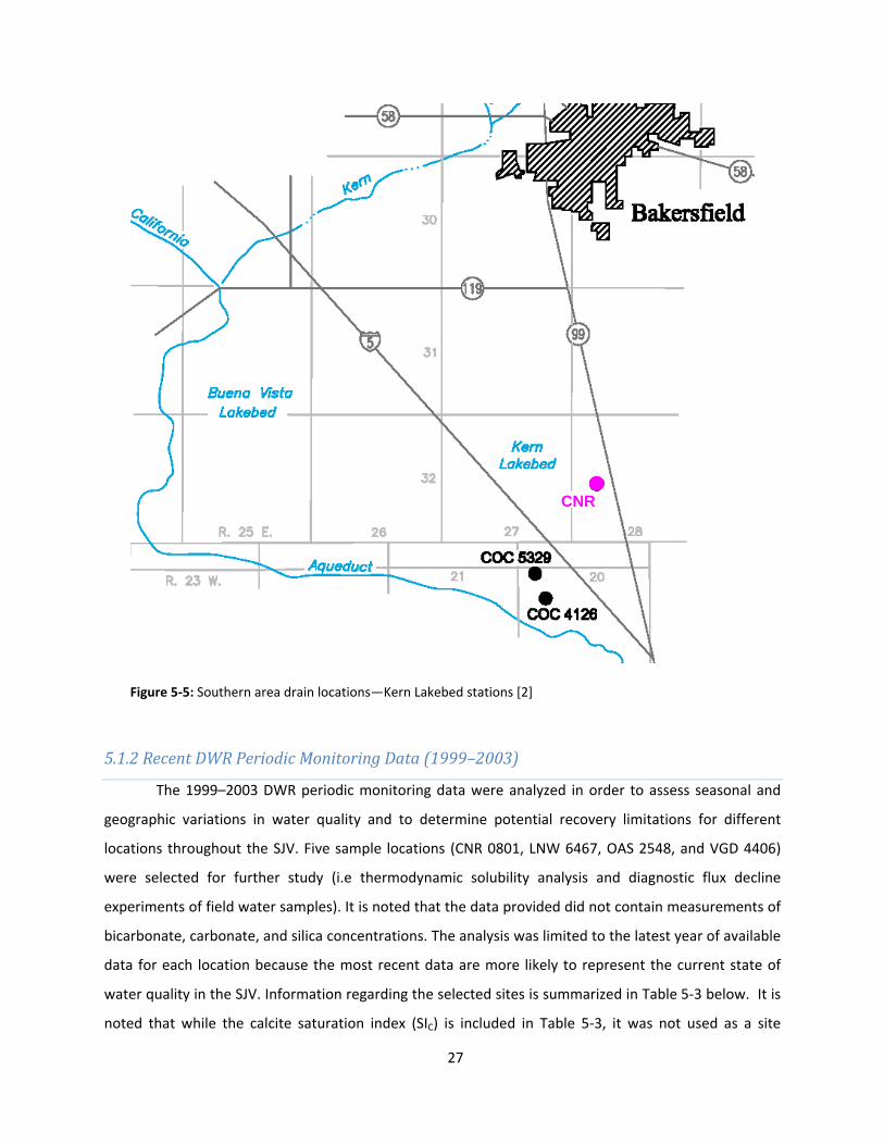
Figure 5‐5: Southern area drain locations—Kern Lakebed stations [2]
5.1.2 Recent DWR Periodic Monitoring Data (1999–2003)
The 1999–2003 DWR periodic monitoring data were analyzed in order to assess seasonal and
geographic variations in water quality and to determine potential recovery limitations for different
locations throughout the SJV. Five sample locations (CNR 0801, LNW 6467, OAS 2548, and VGD 4406)
were selected for further study (i.e thermodynamic solubility analysis and diagnostic flux decline
experiments of field water samples). It is noted that the data provided did not contain measurements of
bicarbonate, carbonate, and silica concentrations. The analysis was limited to the latest year of available
data for each location because the most recent data are more likely to represent the current state of
water quality in the SJV. Information regarding the selected sites is summarized in Table 5‐3 below. It is
noted that while the calcite saturation index (SIC) is included in Table 5‐3, it was not used as a site
CNR

28
selection criterion because SIC is strongly dependant on pH which varies significantly among the
sampling dates and locations. Changes in SIC can largely be attributed to pH variations while changes in
SIG are largely due to changes in water composition (e.g. changes in calcium or sulfate concentrations).
Instead, as shown later in this section, solubility analyses were performed for all locations at two
standardized pH values of 7.5 (near the natural pH of most of the water samples) and 6.0 (a sufficiently
low pH level for suppressing calcite scaling).
Table 5‐3. Summary of average water quality for the most recent year of data (2003–2004)†
Name Location TDS, mg/L
pH [Total Carbonate]‡ / [SO4
2‐], mol/mol SIC
(20ºC) SIG
(20ºC)
CNR 0801 Southern Area, Kern Lake Bed
6,987 7.7 0.1130 5.05 0.758
LNW 6467 Southern Area, Lost Hills
11,944 7.5 0.0534 2.31 0.987
OAS 2548 Central Area 7,999 7.7 0.0967 3.89 0.748
VGD 4406 Southern Area, Lemoore
23,480 7.9 0.0483 5.29 0.844
ERR 8429 Southern Area, Corcoran
4,690 ‐‐ ‐‐ ‐‐ ‐‐
† TDS, pH, and [SO42‐] were obtained from analytical reports, while SIC and SIG were calculated based on the
water composition, ‡ [Total Carbonate] was calculated assuming HCO3‐ was the only species contributing to the
total alkalinity, ‐‐ insufficient data available for calculation
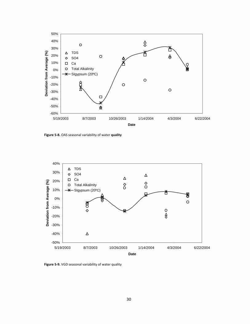
5.1.2.1 Seasonal Variability of Water Quality
The variation of SIG was plotted versus sample date over the latest year of data along with TDS,
total alkalinity, Calcium ion, and Sulfate ion. The temporal variability of water quality is illustrated in
Figures 5‐6 through 5‐9 in plots of percent deviation of water quality indicators and SIG from the
respective annual average values versus time over the latest year of available data for each location.

29
-40%
-30%
-20%
-10%
0%
10%
20%
30%
40%
50%
5/19/2003 8/7/2003 10/26/2003 1/14/2004 4/3/2004 6/22/2004
Date
Dev
iatio
n fr
om A
vera
ge (%
)TDSSO4CaTotal AlkalinitySIgypsum (20ºC)
Figure 5‐6. CNR seasonal variability of water quality
-15%
-10%
-5%
0%
5%
10%
15%
2/28/2003 5/19/2003 8/7/2003 10/26/2003 1/14/2004 4/3/2004
Date
Dev
iatio
n fr
om A
vera
ge (%
)
TDSSO4CaTotal AlkalinitySIgypsum (20ºC)
Figure 5‐7. LNW seasonal variability of water quality
30
-60%
-50%
-40%
-30%
-20%
-10%
0%
10%
20%
30%
40%
50%
5/19/2003 8/7/2003 10/26/2003 1/14/2004 4/3/2004 6/22/2004
Date
Dev
iatio
n fr
om A
vera
ge (%
) TDSSO4CaTotal AlkalinitySIgypsum (20ºC)
Figure 5‐8. OAS seasonal variability of water quality
-50%
-40%
-30%
-20%
-10%
0%
10%
20%
30%
40%
5/19/2003 8/7/2003 10/26/2003 1/14/2004 4/3/2004 6/22/2004
Date
Dev
iatio
n fr
om A
vera
ge (%
)
TDSSO4CaTotal AlkalinitySIgypsum (20ºC)
Figure 5‐9. VGD seasonal variability of water quality
31
As illustrated in Figures 5‐6 through 5‐9, the brackish water quality varied significantly over the
course of a year for each of the selected location in the SJV both seasonally and geographically. One
might expect SIG to increase with TDS, calcium concentration, and/or sulfate concentration. No
consistent seasonal variations were found across the sample locations and no consistent correlation
between SIG and TDS was found for any of the locations. However, the variation of SIG appears to closely
match the variation in calcium concentration. The average TDS for the selected locations ranged from
6987 mg/L to 23,480 mg/L for CNR and VGD, respectively, while the maximum absolute percent
deviation of TDS from the average values ranged from 12% to 52% for LNW and OAS, respectively. The
average calcium ion concentrations ranged from 356 mg/L to 606 mg/L for OAS and LNW, respectively,
and do not correlate with the low and high average TDS values. The maximum absolute percent
deviation of calcium ion concentration from the average values ranged from 7.4% to 37% for LNW and
OAS, respectively. SIG varied from 0.75 to 0.99 (OAS and LNW, respectively), neither of which
corresponds to the low or high measured TDS. The maximum absolute percent deviation of SIG from the
average values ranged from 5.2% to 45% for CNR and OAS, respectively. The lack of correspondence
between SIG and TDS illustrates the variability in water chemistry over time at each location. The low
and high values for average sulfate ion concentration, 4880 mg/L and 16,062 mg/L (LNW and VGD,
respectively) do, however, correspond with the low and high average TDS values. This correspondence is
reasonable even for waters of varying composition because the sulfate ion is the largest single
contributor to TDS for each location, contributing to it by a large majority (from 60% to 68%) for all
locations except for LNW (41%). The maximum absolute percent deviation of sulfate ion concentration
from the average values ranged from 9.6% to 51% for LNW and OAS, respectively. Overall, OAS exhibits
the most variability in water quality of the selected sites, while LNW exhibits the least variability.
5.1.2.2 pH Dependence of Saturation Indices
The relationship between pH and saturation indices for gypsum, calcite, and barite are shown in
Figures 5‐12 through 5‐19 for each of the four selected locations for both the high and low annual TDS
conditions listed in Table 5‐2. The values for barite are provided for illustrative purposes only because
the barium concentrations were reported at or below the detection limits which vary between 0.25 to
1.0 mg/L. The actual barium concentrations may be much lower, thus, the calculated barite saturation
indices are upper limits that may not reflect the recovery limits.
As illustrated in Figures 5‐12 through 5‐19, the saturation index of calcite is highly pH
dependant, increasing by several orders of magnitude over the pH range shown (pH 4 to 6), while the

32
gypsum saturation index decreases by less than 14% over the same range and the barite saturation
index changes by less than 5% over the same pH range except for the CNR location at the high TDS
condition and OAS at the low TDS condition for which the decreases in gypsum saturation index were
18% and 22%, respectively. Because the saturation indices of gypsum, calcite, and barite vary to
different degrees, different strategies must be used to manage their scaling. Calcite scaling can generally
be managed by reducing the pH of the feed water, while barite and gypsum are relatively pH insensitive
and can be partially managed with antiscalant use.
0.00001
0.0001
0.001
0.01
0.1
1
10
100
1000
4 5 6 7 8 9 10
pH
Satu
ratio
n In
dex
BariteCalciteGypsum
Figure 5‐10. Mineral salt solubility dependence on pH for CNR for the high TDS condition (9163 mg/L, 11/12/2003)

33
0.00001
0.0001
0.001
0.01
0.1
1
10
100
1000
4 5 6 7 8 9 10
pH
Satu
ratio
n In
dex
BariteCalciteGypsum
Figure 5‐11. Mineral salt solubility dependence on pH for CNR for the low TDS condition (4660 mg/L, 7/28/2003)
0.00001
0.0001
0.001
0.01
0.1
1
10
100
1000
4 5 6 7 8 9 10
pH
Satu
ratio
n In
dex
BariteCalciteGypsum
Figure 5‐12. Mineral salt solubility dependence on pH for LNW for the high TDS condition (13,400 mg/L, 9/9/2003)

34
0.00001
0.0001
0.001
0.01
0.1
1
10
100
1000
4 5 6 7 8 9 10
pH
Satu
ratio
n In
dex
BariteCalciteGypsum
Figure 5‐13. Mineral salt solubility dependence on pH for LNW for the low TDS condition (11,030 mg/L, 7/28/2003)
0.00001
0.0001
0.001
0.01
0.1
1
10
100
1000
4 5 6 7 8 9 10
pH
Satu
ratio
n In
dex
BariteCalciteGypsum
Figure 5‐14. Mineral salt solubility dependence on pH for OAS for the high TDS condition (11,100 mg/L, 1/12/2004)

35
0.00001
0.0001
0.001
0.01
0.1
1
10
100
1000
4 5 6 7 8 9 10
pH
Satu
ratio
n In
dex
BariteCalciteGypsum
Figure 5‐15. Mineral salt solubility dependence on pH for OAS for the low TDS condition (3828 mg/L, 9/9/2003)
0.00001
0.0001
0.001
0.01
0.1
1
10
100
1000
4 5 6 7 8 9 10
pH
Satu
ratio
n In
dex
BariteCalciteGypsum
Figure 5‐16. Mineral salt solubility dependence on pH for VGD for the high TDS condition (29,760 mg/L, 1/13/2004)

36
0.00001
0.0001
0.001
0.01
0.1
1
10
100
1000
4 5 6 7 8 9 10
pH
Satu
ratio
n In
dex
BariteCalciteGypsum
Figure 5‐17. Mineral salt solubility dependence on pH for VGD for the low TDS condition (14,110 mg/L, 7/29/2003)
5.1.2.3 Recovery Limits
RO recovery limits based on scaling were determined by calculating the recoveries at which the
concentrations of sparingly soluble salts (e.g. calcite, gypsum, barite) reach their maximum controllable
(i.e. non‐scaling) saturation levels. Calcite scaling can be controlled by pH adjustment to saturation or
below and thus SIC equal to unity was set as the upper limit. Gypsum and barite scaling can be controlled
up to SIs of 2.3 and 90, respectively, with antiscalant use. SIC, SIG, and SIB were calculated for a range of
concentration factors (CF; see Eq. 2‐6) for the five selected locations (except for ERR for which there was
insufficient data; Table 5‐2) to determine recovery limits. The change in SI with recovery was then
calculated and plotted by converting the CF values to equivalent recoveries using Equation 2‐7,
SW RCF
CFR+−−
=1
1 (2‐7)
where RW is the fractional product water recovery, CF is the concentration factor, and RS is the fractional
salt rejection. The results of the above analysis are summarized in Figures 5‐18 through 5‐33 where the
pH was held constant first at 7.5 and then at 6.0 by addition of sodium hydroxide or hydrochloric acid.
Because all of the water samples had a natural pH in the range 7.1–8.1, an average pH of 7.5 was
selected as a reasonable value for an “untreated” water and a pH of 6.0 was selected as an adjusted
feed pH representative of the condition for controlling calcite scaling.

37
0.01
0.1
1
10
100
1000
0 0.1 0.2 0.3 0.4 0.5 0.6 0.7 0.8 0.9
Fractional Recovery
Satu
ratio
n In
dex
BaSO4CaSO4.2H2OCaCO3
Figure 5‐18. Saturation indices vs recovery (CNR, TDS 9136, pH 7.5)
0.01
0.1
1
10
100
1000
0 0.1 0.2 0.3 0.4 0.5 0.6 0.7 0.8 0.9
Fractional Recovery
Satu
ratio
n In
dex
BaSO4CaSO4.2H2OCaCO3
Figure 5‐19. Saturation indices vs recovery (CNR, TDS 9136, pH 6.0)

38
0.01
0.1
1
10
100
1000
0 0.1 0.2 0.3 0.4 0.5 0.6 0.7 0.8 0.9
Fractional Recovery
Satu
ratio
n In
dex
BaSO4CaSO4.2H2OCaCO3
Figure 5‐20. Saturation indices vs recovery (CNR, TDS 4660, pH 7.5)
0.01
0.1
1
10
100
1000
0 0.1 0.2 0.3 0.4 0.5 0.6 0.7 0.8 0.9
Fractional Recovery
Satu
ratio
n In
dex
BaSO4CaSO4.2H2OCaCO3
`
Figure 5‐21. Saturation indices vs recovery (CNR, TDS 4660, pH 6.0)

39
0.01
0.1
1
10
100
1000
10000
0 0.1 0.2 0.3 0.4 0.5 0.6 0.7 0.8 0.9
Fractional Recovery
Satu
ratio
n In
dex
BaSO4CaSO4.2H2OCaCO3
Figure 5‐22. Saturation indices vs recovery (LNW, TDS 13400, pH 7.5)
0.01
0.1
1
10
100
1000
10000
0 0.1 0.2 0.3 0.4 0.5 0.6 0.7 0.8 0.9
Fractional Recovery
Satu
ratio
n In
dex
BaSO4CaSO4.2H2OCaCO3
Figure 5‐23. Saturation indices vs recovery (LNW, TDS 13400, pH 6.0)
40
0.01
0.1
1
10
100
1000
10000
0 0.1 0.2 0.3 0.4 0.5 0.6 0.7 0.8 0.9
Fractional Recovery
Satu
ratio
n In
dex
BaSO4CaSO4.2H2OCaCO3
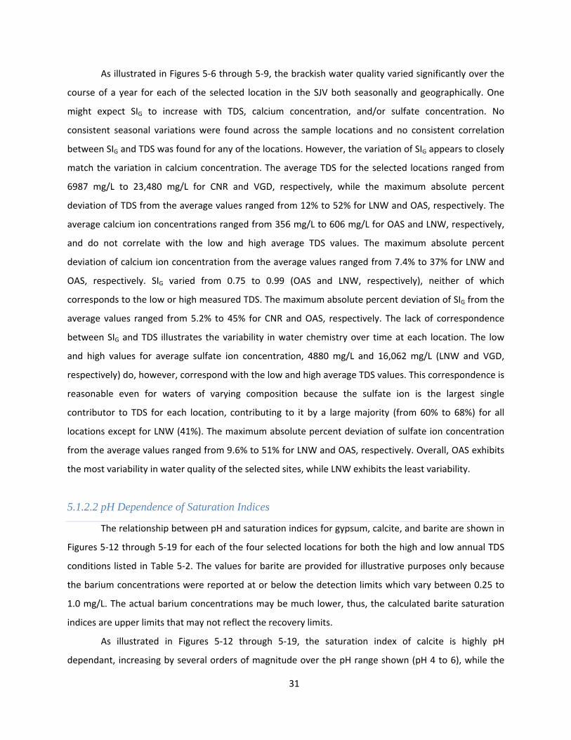
Figure 5‐24. Saturation indices vs recovery (LNW, TDS 11030, pH 7.5)
0.01
0.1
1
10
100
1000
10000
0 0.1 0.2 0.3 0.4 0.5 0.6 0.7 0.8 0.9
Fractional Recovery
Satu
ratio
n In
dex
BaSO4CaSO4.2H2OCaCO3
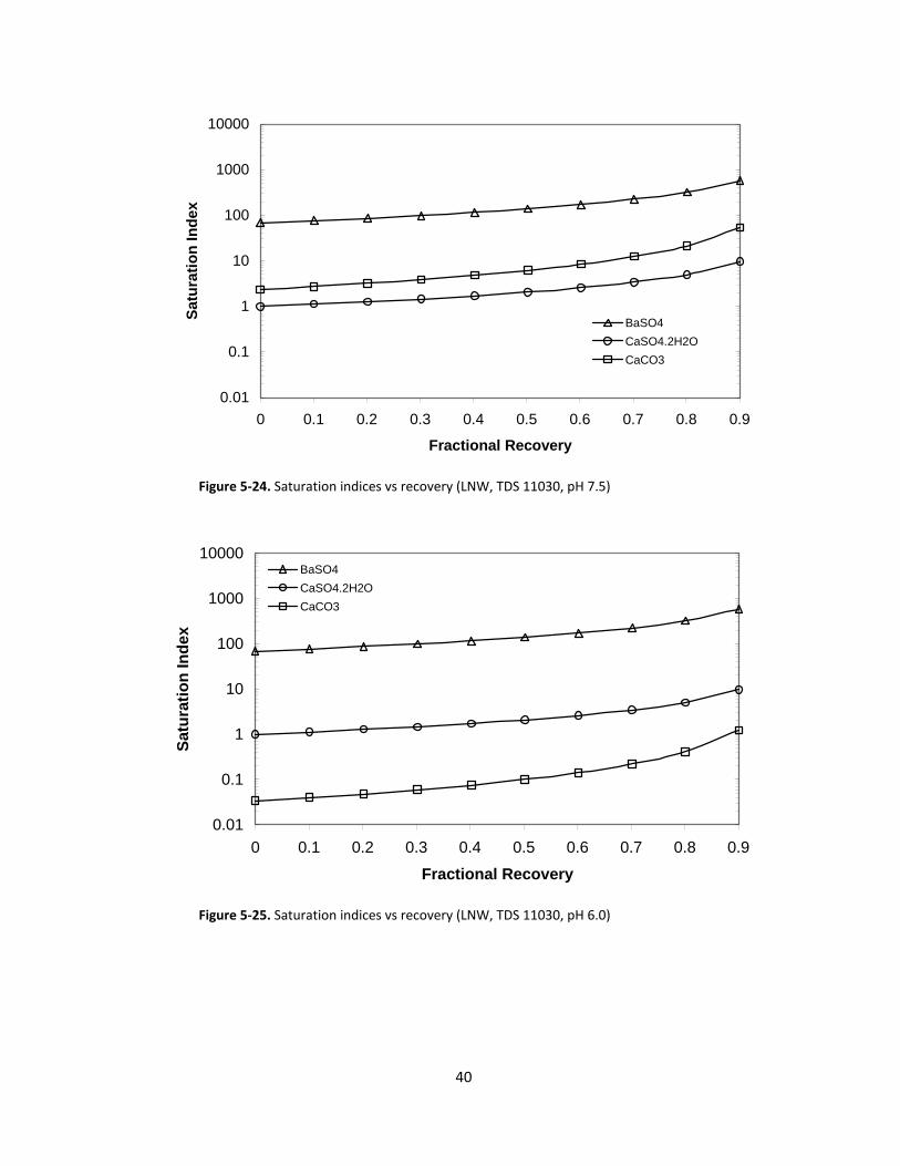
Figure 5‐25. Saturation indices vs recovery (LNW, TDS 11030, pH 6.0)

41
0.01
0.1
1
10
100
1000
10000
0 0.1 0.2 0.3 0.4 0.5 0.6 0.7 0.8 0.9
Fractional Recovery
Satu
ratio
n In
dex
BaSO4CaSO4.2H2OCaCO3
Figure 5‐26. Saturation indices vs recovery (OAS, TDS 11100, pH 7.5)
0.01
0.1
1
10
100
1000
10000
0 0.1 0.2 0.3 0.4 0.5 0.6 0.7 0.8 0.9
Fractional Recovery
Satu
ratio
n In
dex
BaSO4CaSO4.2H2OCaCO3
Figure 5‐27. Saturation indices vs recovery (OAS, TDS 11100, pH 6.0)

42
0.01
0.1
1
10
100
1000
10000
0 0.1 0.2 0.3 0.4 0.5 0.6 0.7 0.8 0.9
Fractional Recovery
Satu
ratio
n In
dex
BaSO4CaSO4.2H2OCaCO3
Figure 5‐28. Saturation indices vs recovery (OAS, TDS 3828, pH 7.5)
0.01
0.1
1
10
100
1000
10000
0 0.1 0.2 0.3 0.4 0.5 0.6 0.7 0.8 0.9
Fractional Recovery
Satu
ratio
n In
dex
BaSO4CaSO4.2H2OCaCO3
Figure 5‐29. Saturation indices vs recovery (OAS, TDS 3828, pH 6.0)
43
0.01
0.1
1
10
100
1000
10000
0 0.1 0.2 0.3 0.4 0.5 0.6 0.7 0.8 0.9
Fractional Recovery
Satu
ratio
n In
dex
BaSO4CaSO4.2H2OCaCO3
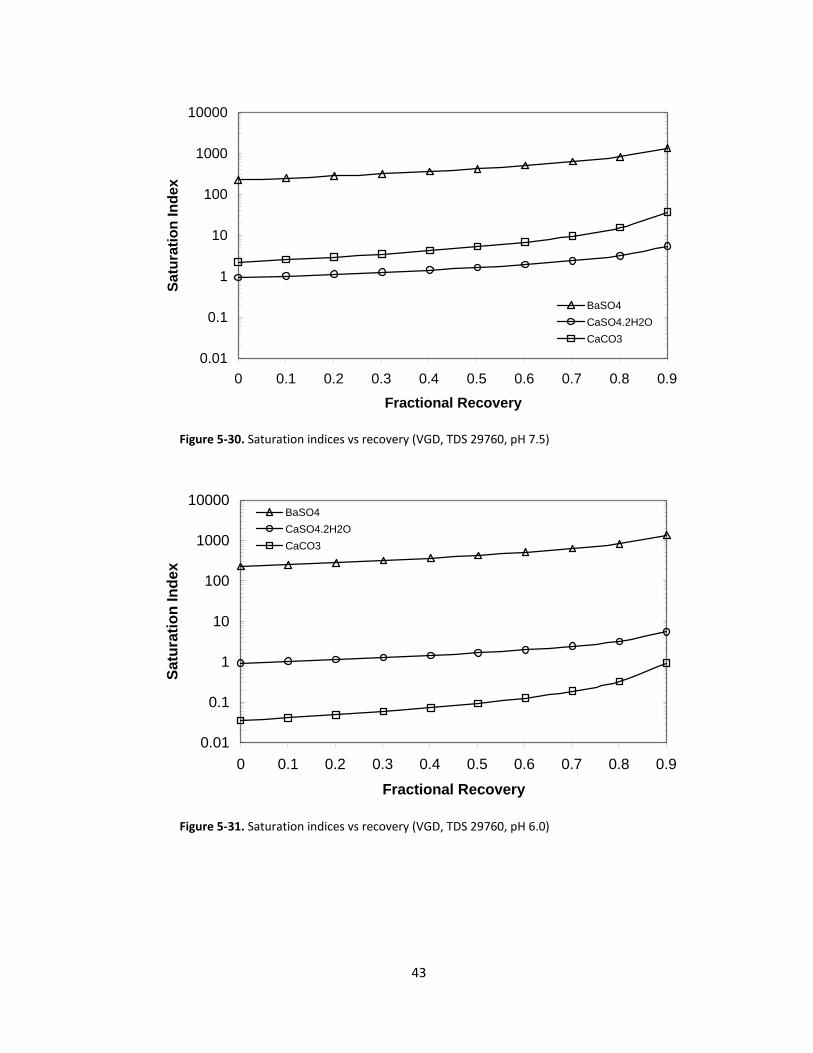
Figure 5‐30. Saturation indices vs recovery (VGD, TDS 29760, pH 7.5)
0.01
0.1
1
10
100
1000
10000
0 0.1 0.2 0.3 0.4 0.5 0.6 0.7 0.8 0.9
Fractional Recovery
Satu
ratio
n In
dex
BaSO4CaSO4.2H2OCaCO3
Figure 5‐31. Saturation indices vs recovery (VGD, TDS 29760, pH 6.0)

44
0.01
0.1
1
10
100
1000
10000
0 0.1 0.2 0.3 0.4 0.5 0.6 0.7 0.8 0.9
Fractional Recovery
Satu
ratio
n In
dex
BaSO4CaSO4.2H2OCaCO3
Figure 5‐32. Saturation indices vs recovery (VGD, TDS 14110, pH 7.5)
0.01
0.1
1
10
100
1000
10000
0 0.1 0.2 0.3 0.4 0.5 0.6 0.7 0.8 0.9
Fractional Recovery
Satu
ratio
n In
dex
BaSO4CaSO4.2H2OCaCO3
Figure 5‐33. Saturation indices vs recovery (VGD, TDS 14110, pH 6.0)
As illustrated in Figures 5‐18 through 5‐33, SIB, SIC, and SIG all increase with increasing recovery
as would be expected. When comparing the SI values at pH 7.5 to those at pH 6.0, it is apparent that SIG
and SIB do not vary significantly with pH (increasing less than 3 % and 1.5 % for SIG and SIB, respectively,

45
at 90 % recovery), while SIC changes by nearly two orders of magnitude (decreasing by at least a factor
of 40 at 90 % recovery) over the pH range of 7.5 to 6.0. It is noteworthy that at high recoveries the SIs
for all scalants increase rapidly with increasing recovery. The SIs increase by about the same factor from
between zero and 65 % recovery as they do from between 65 % and 90 % recovery.
The product water recovery limits were calculated with respect to gypsum and calcite for each
of the four sample locations for both the samples having the highest TDS during the latest year of
available data and for the samples having the lowest TDS over the same period. Both high and low TDS
conditions were selected to illustrate the impact of seasonal variability on the recovery limits that are
likely to be encountered for RO desalting of inland brackish water in the SJV. Recovery limits were
calculated at a pH of 7.5 and 6.0 for comparison as shown in Table 5‐4. Note that because there is no
direct correlation between TDS and SI (i.e. water having the highest TDS does not necessarily have the
highest SI), Table 5‐4 may not necessarily contain the best and worst case recovery limits for each site.
Nonetheless, TDS was selected as the basis for comparison of high and low recovery limits in the present
study because TDS can be quickly and easily measured in field RO desalting operations, while SI
calculations require complete water composition which can take weeks to acquire.
Table 5‐4. Recovery limits (SI = 1) with respect to gypsum and calcite at pH = 7.5 and 6.0 for water samples having the max and min TDS observed during the latest year of reported data [11].
Recovery Limits
pH =7.5 pH = 6.0 Site Sample Date TDS gypsum calcite gypsum calcite
CNR 0801 11/12/2003 9136 25% 0% 24% 86% CNR 0801 7/28/2003 4660 20% 0% 19% 88% LNW 6467 9/9/2003 13400 0% 0% 0% 86% LNW 6467 7/28/2003 11030 0.33% 0% 0.002% 87% OAS 2548 1/12/2004 11100 0% 0% 0% 93% OAS 2548 9/9/2003 3828 54% 0% 53% 90% VGD 4406 1/13/2004 29760 8.5% 0% 7.6% 91% VGD 4406 7/29/2003 14110 19% 0% 18% 92%
All water samples are saturated or near saturated with gypsum and oversaturated with calcite
and barite at a pH of 7.5 (near the natural pH of the water samples), thus calcite scaling would limit the
water recovery for each location. When the pH is lowered to 6.0, gypsum becomes the limiting scalant
with respect to recovery. Barite scaling is not expected to be a limiting factor because, even though the
water is oversaturated in barite, Barium is present at very low concentrations at or below detection
limits and the total mass of barite that could scale is very small. Also, experience shows that because of
the slow kinetics of barium sulfate, precipitation is not a problem at the residence times typically

46
observed in RO desalination units [20, 28, 35]. The recovery limits with respect to scaling for each water
sample location are summarized below.
i. CNR 0801 (2003 –2004)
The percent recovery limit (i.e. at SIG = 1.0) at this location is 24 % for the highest observed TDS
(9136 mg/L) and 19 % for the lowest TDS (4660 mg/L) at a pH of 6.0. It is noteworthy that the percent
recovery limit imposed by gypsum is actually higher at the higher TDS because of variations in water
composition between the samples.
ii. LNW 6467 (2003 –2004)
Of the four locations analyzed, the lowest recovery limit would be expected at this location
based on gypsum scaling (highest average SIG of all locations was 0.99) with SIG ranging from 0.91 to 1.03
over the course of a year. The water sample with the highest TDS observed over the latest year (13,400
mg/L) is oversaturated in gypsum (SIG = 1.03), thus RO desalting would not be feasible without scale
mitigation. At the lowest TDS, RO desalting at this site would be limited to a recovery of 0.002 %. Water
from this location would require pretreatment and/or antiscalants to achieve any reasonable product
water recovery.
iii. OAS 2548 (2003 –2004)
This location had the largest range of recovery limits based on gypsum scaling from zero % at
the high TDS (11,100 mg/L) to 53 % at the low TDS (3828 mg/L), corresponding to both the highest and
lowest recoveries observed at all four locations.
iv. VGD 4406 (2003 –2004)
This location had the highest observed TDS (29,760 mg/L) of all four sample locations, even its
minimum TDS (14,110 mg/L) during the latest year of available data is higher than the maximum TDS
seen at any of the other three locations (13,400 mg/L at LNW). However, when compared to the
recoveries at each location’s high TDS value, the recovery limit at this location is 7.6% which is greater
than two of the other locations, LNW and OAS, which have TDS values less than half of VGD’s value.
Also, at VGD’s low TDS, the recovery limit is 18%, which is higher than the recovery limit at LNW
(0.002%) and nearly as high as the CNR (19%).
5.1.3 Field Water Sample Data (2006–2007) The more recent water quality data was provided by DWR in 25‐gallon water samples for each
of the five chosen sites for analysis. A summary of the data and the detailed water quality analyses for
the five locations and are shown in Tables 5‐5 and 5‐6, respectively.

47
Table 5‐5. Field sample water quality and SI summary (2006–2007)
Name Sample Date
Location TDS, mg/L
pH Total Alk,
mg/L as CaCO3 SIC SIG SIS
CNR 0801 7/31/2006 Southern Area, Kern Lakebed 6372 7.5 230 2.70 0.704 0.222
LNW 6467 2/15/2006 Southern Area, Lost Hills 11270 7.6 128 2.72 1.03 0.345
OAS 2548 4/10/2006 Central Area 11020 7.6 213 3.02 0.985 0.287
VGD 4406 11/13/2006 Southern Area, Lemoore 28780 7.6 368 2.18 0.953 0.377
ERR 8429 1/29/2007 Southern Area, Corcoran 4115 8.0 706 9.50 0.120 0.339
Note: Values are those measured on the sampling date. Table 5‐6. Detailed water quality analyses (2006–2007)
Measurement Units Location CNR LNW OAS VGD ERR Conductance μS/cm 7111 14430 12620 26070 5580 pH pH units 7.5 7.6 7.6 7.6 8 UV Absorbance (254 nm) absorbance/cm 0.126 0.094 0.13 0.178 0.587
Dissolved Measurements Bicarbonate mg/L as CaCO3 229 128 212 367 699 Boron mg/L 13.5 17.5 23.5 43.4 2.6 Calcium mg/L 350 625 462 422 88 Carbonate mg/L as CaCO3 1* 1* 1* 1* 7 Chloride mg/L 324 3020 1060 1910 632 Fluoride mg/L 5* 10* 10* 5* 5* Hydroxide mg/L as CaCO3 1* 1* 1* 1* 1* Magnesium mg/L 236 198 284 962 59 Nitrate mg/L 344 155 46.7 51.9 51.3 DOC mg/L as C 4.2 4.6 5.1 6.2 15.8 Potassium mg/L 46.7 5* 5* 7.8 3.5 Selenium mg/L 0.032 0.223 0.184 0.05* 0.011 Silica mg/L 23.5 37.9 31.4 43.2 38 Sodium mg/L 1250 2820 2780 9270 1250 Sulfate mg/L 3700 4520 6360 21400 1570
Total Measurements Total Alkalinity mg/L as CaCO3 230 128 213 368 706 Aluminum mg/L 0.1* 0.1* 0.05* 0.5* 0.102 Arsenic mg/L 0.01* 0.014 0.006 0.05* 0.089 Barium mg/L 0.5* 0.5* 0.25* 2.5* 0.5* TDS mg/L 6372 11270 11020 28780 4115 Iron mg/L 0.174 0.152 0.045 1.41 0.279 Manganese mg/L 0.05* 0.05* 0.025* 1.55 0.595 TOC mg/L as C 4.5 3.4 5.1 6.2 16.7 Phosphorus mg/L 0.01* 0.03 0.08 0.12 1.96 Selenium mg/L 0.034 0.235 0.195 0.05* 0.013 Strontium mg/L 17.2 9.96 5.5 9.6 0.898 TSS mg/L 1* 4 4 2 4
* Measured value is at or below reporting limit.

48
5.1.3.1 pH Dependence of Saturation Indices The saturation indices of sparingly soluble salts depend on pH to varying degrees. The
relationship between pH and SI (at 20 ºC) is shown in Figs 5‐36 through 5‐40 for gypsum, calcite, barite,
and silica for field water samples from each of the locations listed in Table 5‐5. The values for barite are
provided for illustrative purposes only because the barium concentration is known only to be at or
below the detection limits which vary between 0.25 to 1.0 mg/L. The actual barium concentrations may
be much lower.
As illustrated previously in Figures 4‐11 through 4‐18 for the recent water quality data (2003–2004),
Figures 5‐36 through 5‐40 illustrate, for the field water sample data (2006–2007), that SIC is pH sensitive,
increasing by several orders of magnitude over the pH range shown (4 to 10), while SIG decreases by less
than 15% and SIB changes by less than 3% over the same pH range of 4 to 10 (except for water from ERR
where the SIG and SIB decrease by 58% and 22%, respectively). The silica saturation index (SIS) at each
location decreases by more than one order of magnitude over the same pH range of 4 to 10.
0.00001
0.0001
0.001
0.01
0.1
1
10
100
1000
4 5 6 7 8 9 10
pH
Satu
ratio
n In
dex
BariteCalciteGypsumSilica
Figure 5‐36. Mineral salt solubility dependence on pH for CNR field water sample (see Table 5‐6)

49
0.00001
0.0001
0.001
0.01
0.1
1
10
100
1000
4 5 6 7 8 9 10
pH
Satu
ratio
n In
dex
BariteCalciteGypsumSilica
Figure 5‐37. Mineral salt solubility dependence on pH for ERR field water sample (see Table 5‐6)
0.00001
0.0001
0.001
0.01
0.1
1
10
100
1000
4 5 6 7 8 9 10
pH
Satu
ratio
n In
dex
BariteCalciteGypsumSilica
Figure 5‐38. Mineral salt solubility dependence on pH for LNW field water sample (see Table 5‐6)

50
0.00001
0.0001
0.001
0.01
0.1
1
10
100
1000
4 5 6 7 8 9 10
pH
Satu
ratio
n In
dex
BariteCalciteGypsumSilica
Figure 5‐39. Mineral salt solubility dependence on pH for OAS field water sample (see Table 5‐6)
0.00001
0.0001
0.001
0.01
0.1
1
10
100
1000
4 5 6 7 8 9 10
pH
Satu
ratio
n In
dex
BariteCalciteGypsumSilica
Figure 5‐40. Mineral salt solubility dependence on pH for VGD field water sample (see Table 5‐6)

51
5.1.3.2 Recovery Limits
SIC, SIG, and SIS were calculated as a function of the product water recoveries. The analysis was
carried out by holding the pH constant first at the water’s natural pH and then at 6.0 by addition of
sodium hydroxide or hydrochloric acid as needed. The above pH conditions were chosen for each
location to illustrate the effectiveness of pH reduction on increasing the recovery limits with respect to
calcite as is the common practice in RO desalination plants.
0.01
0.1
1
10
100
1000
0 0.1 0.2 0.3 0.4 0.5 0.6 0.7 0.8 0.9
Fractional Recovery
Satu
ratio
n In
dex
calcite, pH 7.6gypsum, pH 7.6silica, pH 7.6calcite, pH 6.0gypsum, pH 6.0silica, pH 6.0
Figure 5‐41. VGD field water saturation indices as a function of recovery (see Table 5‐6)

52
0.01
0.1
1
10
100
1000
0 0.1 0.2 0.3 0.4 0.5 0.6 0.7 0.8 0.9
Fractional Recovery
Satu
ratio
n In
dex
calcite, pH 8.0gypsum, pH 8.0silica, pH 8.0calcite, pH 6.0gypsum, pH 6.0silica, pH 6.0
Figure 5‐42. ERR field water saturation indices as a function of recovery (see Table 5‐6)
0.01
0.1
1
10
100
1000
0 0.1 0.2 0.3 0.4 0.5 0.6 0.7 0.8 0.9
Fractional Recovery
Satu
ratio
n In
dex
calcite, pH 7.5gypsum, pH 7.5silica, pH 7.5calcite, pH 6.0gypsum, pH 6.0silica, pH 6.0
Figure 5‐43. CNR field water saturation indices as a function of recovery (see Table 5‐6)

53
0.01
0.1
1
10
100
1000
0 0.1 0.2 0.3 0.4 0.5 0.6 0.7 0.8 0.9
Fractional Recovery
Satu
ratio
n In
dex
calcite, pH 7.6gypsum, pH 7.6silica, pH 7.6calcite, pH 6.0gypsum, pH 6.0silica, pH 6.0
Figure 5‐44. OAS field water saturation indices as a function of recovery (see Table 5‐6)
0.01
0.1
1
10
100
1000
0 0.1 0.2 0.3 0.4 0.5 0.6 0.7 0.8 0.9
Fractional Recovery
Satu
ratio
n In
dex
calcite, pH 7.6gypsum, pH 7.6silica, pH 7.6calcite, pH 6.0gypsum, pH 6.0silica, pH 6.0
Figure 5‐45. LNW field water saturation indices as a function of recovery (see Table 5‐6)

54
The RO product water recovery limits were calculated with respect to potential scaling by
gypsum, calcite, and silica for field water samples from each of the five sample locations (Table 5‐2).
Calcite and silica recovery limits were calculated at the natural pH of the field samples and at a reduced
pH of about 6.0 so as to compare the recovery limits with and without pH adjustment. Additionally, the
recovery limit associated gypsum for SI = 1 and SI = 2.3 were determined in order to compare the
recovery limits with and without antiscalant addition. Two possible osmotic pressure recovery limits
were also calculated as the recovery at which the osmotic pressure equals 600 and 1000 psi—two
common maximum operating pressures for RO pressure vessels.
Table 5‐7. Field water sample recovery limits Pressure Recovery Limits Scaling Recovery Limits Site TDS,
mg/L Nat pH
π = 600 psi π =1000 psi Calcite (nat pH)
Calcite (pH 6)
Gypsum (pH 6)
Gypsum (pH 6)
Silica (pH 6)
SI = 1 SI = 1 SI = 1 SI = 2.3 SI = 1 VGD 28780 7.6 69.9% 81.4% oversat. 91.1% 6.17% 67.0% 54.9%ERR 4116 8.0 94.3% 96.5% oversat. 88.2% 85.3% 94.0% 63.4%CNR 6372 7.5 94.3% 96.5% oversat. 91.0% 27.3% 68.2% 77.0%OAS 11020 7.6 88.9% 93.1% oversat. 91.1% 0.70% 57.9% 68.9%LNW 11270 7.6 83.2% 89.6% oversat. 90.0% oversat. 53.6% 62.1%
Note: Bold values are the ultimate recovery limits with pH adjustment and antiscalant use.
Brackish water from each of the five locations is oversaturated with respect to calcite at the
natural pH levels. Therefore, without pH adjustment, RO desalting of water at any of the five locations
(Table 5‐2) would not yield product water without risking scaling the membranes with calcite. When the
pH is adjusted to 6.0 (e.g. by acid addition), the calcite scaling recovery limits increase to 88.2%–91.1%
due to the elimination of calcite scaling. Since calcite scaling can be controlled by pH adjustment,
gypsum scaling is the next important recovery limiting scalant. Without the use of antiscalants, gypsum
scaling would limit the recovery for each location except for ERR which would still be limited by
potential silica scaling (at pH = 6.0). It is noted that water at LNW is oversaturated with respect to
gypsum. However, because gypsum scaling can be controlled with appropriate antiscalant addition up to
SIG = 2.3, the recovery limits could be greatly increased (with antiscalant use) to between 53.6% and
94.0%. Silica scaling would limit recovery to the range of 54.9%–77.0%. The recovery limits at osmotic
pressures of 600 psi and 1000 psi are in the range of 69.9%–94.3% (600 psi) and 81.4%–96.5% (1000
psi), respectively. It is noted that even at the lower osmotic pressure limit of 600 psi, scaling remains the
dominant factor that would limit recovery. Practical or economic considerations, however, may lead to a
lower recovery limit depending on the maximum allowable operating pressure.

55
The ultimate recovery limits for each location (with antiscalant use and pH adjustment) are
between 53.6% and 68.2%. Desalting for VGD and ERR source water would be limited by silica scaling to
recoveries of 54.9% and 63.4%, respectively, while at CNR, OAS, and LNW desalting would be limited by
gypsum scaling to recoveries of 68.2%, 57.9%, and 53.6%, respectively.
The analysis of the present study demonstrated that: (1) recovery limits can be estimated for
field water sources prior to pilot studies; (2) potential recovery bottlenecks (e.g. scaling, osmotic
pressure) can be anticipated and pilot study operations can be optimized for a particular water source
and thus assist in the design of pilot studies; (3) pilot and full‐scale RO plants should be designed to
accommodate the expected range of feed water quality reducing the need for costly modifications after
being built. It must be recognized, however, that the present study does not account for recovery
limitations that may be imposed by colloidal fouling, organic fouling, or biofouling.
5.2 Diagnostic Flux Decline Experiments
Diagnostic flux decline experiments were performed on field water samples from the five
selected locations in the San Joaquin Valley (see Table 5‐2, §5.1.1) to assess the feasibility for RO
desalination of water from these locations. The diagnostic experiments were performed for field water
samples rather than model solutions to more closely represent natural conditions with respect to the
source water quality. Three distinct experiments were performed for each field water sample (except for
LNW field water for which only two of the experiments conducted are reported) by changing the initial
conditions of the sample water, while leaving the operating conditions unchanged: (1) at the natural pH
without any adjustment (pH 7.42 to pH 8.02), with adjustment to a low target of pH 6.0 (in practice the
adjusted pH ranged from 5.27 to 6.48), and with adjustment to a low target of pH 6.0 with antiscalant
addition (0.20 ppm PC‐504). The operating conditions for the experiments were selected to impose an
average CP such that over a 24‐hr period substantial flux declines would be observed (see Table 5‐7).
The CP was controlled by adjusting the operating pressure and cross‐flow rates which in turn change the
permeate flux and mass transfer coefficient (see Eq 2‐3).
The flux decline for each run was measured by plotting the relative flux (the flux at a given time
divided by the initial flux) versus time. Although most of the runs were started at nearly the same initial
flux (within 2%), and considering that in some cases the final flux decline was small (< 10%), the flux
measurements were normalized (with respect to the initial flux) in order to make better comparisons
among all of the runs. The percent flux decline, FD, is defined as:

56
1001 ⋅⎟⎟⎠
⎞⎜⎜⎝
⎛−=
i
f
FF
FD (5‐1)
where, Ff and Fi are the final and initial fluxes, respectively.
The initial average SI values for calcite, gypsum, and silica, at the membrane surface (SIM,C, SIM,G,
and SIM,S, respectively), were calculated by first estimating the average CP (CPavg) for each run and then
calculating the initial SI values at the new concentration by using CPavg as a concentration factor (see Eq
3‐1, §3.2). CPavg was estimated by the finite element numerical model developed by Lyster and Cohen
[26] which considers the fully coupled governing equations for fluid dynamics and mass transfer. A
summary of the experimental conditions and the observed final 24‐hour flux declines is provided below.
Table 5‐8. Diagnostic flux decline experimental conditions and 24‐hour flux decline Site Condition TDS,
mg/L pH x‐flow,
L/min Fi, µm/s
P, psi CPavg SIM,C SIM,G SIM,S FD Rw,eqv
VGD Nat. pH 28780 7.53 0.76 13.60 453 1.60 3.22 1.42 0.606 7.96 % 38%
VGD Low pH 28780 5.56 0.76 13.54 432 1.59 0.0115 1.43 0.712 8.88 % 38%
VGD Low pH+AS
28780 5.93 0.76 13.60 455.5 1.61 0.0447 1.44 0.720 9.36 % 38%
ERR Low pH & AS
4116 6.00 0.76 24.45 276.1 2.12 0.128 0.301 0.787 7.54 % 53%
ERR Low pH 4116 5.37 0.76 24.43 306.5 2.12 0.0105 0.307 0.786 11.6 % 53%
ERR Nat. pH 4116 8.02 0.76 24.46 302.3 2.13 29.3 0.280 0.678 12.4 % 53%
CNR Nat. pH 6375 7.50 0.76 24.41 277.7 2.11 7.37 1.53 0.464 6.37 % 53%
CNR Low pH 6372 5.27 0.76 24.44 270.0 2.11 0.00613
1.55 0.487 11.0 % 53%
CNR Low pH & AS
6372 6.00 0.76 24.42 290.9 2.12 0.111 1.55 0.487 6.73 % 53%
OAS Low pH & AS
11020 5.94 0.76 24.36 349.0 2.11 0.862 2.10 0.660 7.89 % 53%
OAS Low pH 11020 5.47 0.76 24.46 374 2.1 0.0140 2.10 0.657 47.4 % 53%
OAS Nat. pH 11020 7.42 0.76 24.52 362.5 2.1 5.41 2.08 0.613 11.2 % 53%
LNW Low pH 11270 6.48 1.0 18.88 283 1.8 0.368 1.94 0.679 14.2 % 45%
LNW Nat. pH 11270 7.43 1.0 19.08 280.5 1.8 4.24 1.93 0.636 10.7 % 45%
Note: SIM,C, SIM,G, and SIM,S are the initial average values at the membrane surface; x‐flow is the cross‐flow velocity of the feed; P is the applied pressure; RW,eqv is the equivalent recovery (see Eq 3‐2, §3.4).
The results summarized in Table 5‐8 show that the saturation indices and 24‐hr percent flux
declines do not appear to correlate with TDS. The above is not surprising since the specific composition
of the various ions determines the scaling propensity of the water. For each experiment, silica (for the
different source water locations) was undersaturated at the membrane surface with SIM,S ranging from
0.46 (CNR) to 0.79 (ERR). For each sample at its natural pH condition, calcite was above saturation with
SIM,C ranging from 3.22 (VGD) to 29.3 (ERR); after pH adjustment each sample was undersaturated with

57
respect to calcite with SI values ranging from 0.00613 (CNR) to 0.862 (OAS). Gypsum was oversaturated
at the membrane surface in each water sample except for ERR where its SI was around 0.3.
For all of the field water except for VGD and ERR, there was significantly more flux decline at the
lower pH than at the natural pH of the water samples. Although the saturation indices of calcite
decreased by at least an order of magnitude and the saturation indices of gypsum and silica increased
only slightly at the lower pH, there was more flux decline at the lower pH likely due to faster
precipitation kinetics. It has been shown for waters containing both sulfate and bicarbonate, that
bicarbonate can retard gypsum scaling by reducing the appearance and growth rate of crystals on the
membrane surface. When both bicarbonate and antiscalants were present, they were shown to have
acted synergistically to retard gypsum scaling. When considering the antagonistic kinetic effect, a
greater flux decline would be expected at the lower pH because of the greatly reduced bicarbonate
concentrations as seen for CNR, OAS, and LNW. The reduced flux declines observed for all of the
experiments with antiscalant addition may be explained by the synergistic effects of the antiscalant and
bicarbonate acting to retard gypsum scaling [30].
Equivalent recoveries can be calculated for each diagnostic experiment by using Equation 3‐1.
This yields the recovery at which an actual RO module would experience average concentration levels in
its exit region equivalent to those near the membrane in the plate‐and‐frame system. The actual
recoveries for the diagnostic tests were 0.21% for VGD; 0.38% for ERR, CNR, and OAS; and 0.22%–0.23%
for LNW. The equivalent operating recoveries (accounting for CP) for the diagnostic experiments were
38% for VGD; 53% for ERR, CNR, and OAS; and 45% for LNW. These results indicate that with the use of
antiscalants and pH adjustment (e.g. acid addition) an RO process could feasibly operate at least at the
above recovery levels, if not higher, because there was no visible scale present on any of the
membranes under these conditions and the flux declines at these conditions (<10%) was likely due to
residual compaction only.
For the experiments performed with no antiscalant addition, scale was either visible in both the
natural and pH adjusted cases (CNR, OAS, VGD, LNW) or in neither case (ERR). The ERR field water was
the only sample undersaturated with respect to gypsum at the membrane surface for the present RO
operating conditions. This indicates that without the use of antiscalants, whether or not pH adjustment
is incorporated, the recovery of an RO process will be limited by scaling to well below the equivalent
experimental recoveries of 53% (CNR, OAS), 38% (VGD), and 45% (LNW). For ERR, however, the recovery
limit with respect to scaling will likely be at least 53%. Flux decline plots and photographs of the
membrane coupons after the 24‐hour flux decline runs are shown below.
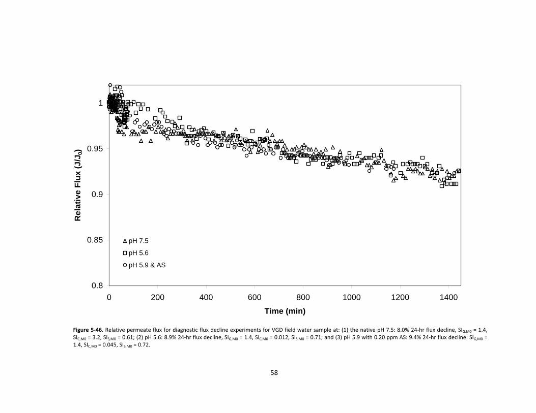
58
0.8
0.85
0.9
0.95
1
0 200 400 600 800 1000 1200 1400
Time (min)
Rel
ativ
e Fl
ux (J
/J0)
pH 7.5
pH 5.6
pH 5.9 & AS
Figure 5‐46. Relative permeate flux for diagnostic flux decline experiments for VGD field water sample at: (1) the native pH 7.5: 8.0% 24‐hr flux decline, SIG,M0 = 1.4, SIC,M0 = 3.2, SIS,M0 = 0.61; (2) pH 5.6: 8.9% 24‐hr flux decline, SIG,M0 = 1.4, SIC,M0 = 0.012, SIS,M0 = 0.71; and (3) pH 5.9 with 0.20 ppm AS: 9.4% 24‐hr flux decline: SIG,M0 = 1.4, SIC,M0 = 0.045, SIS,M0 = 0.72.
(1) pH 7.5
(2) pH 5.6
(3) pH 5.9 & AS

59
0.8
0.85
0.9
0.95
1
0 200 400 600 800 1000 1200 1400
Time (min)
Rel
ativ
e Fl
ux (J
/J0)
pH 8.0
pH 5.4
pH 6.0 & AS
Figure 5‐47. Relative permeate flux for diagnostic flux decline experiments for ERR field water sample at: (1) the native pH 8.0: 12.4% 24‐hr flux decline, SIG,M0 = 0.28, SIC,M0 = 29, SIS,M0 = 0.68; (2) pH 5.4: 11.6% 24‐hr flux decline, SIG,M0 = 0.31, SIC,M0 = 0.011, SIS,M0 = 0.79; and (3) pH 6.0 with 0.20 ppm AS: 7.5% 24‐hr flux decline, SIG,M0 = 0.30, SIC,M0 = 0.13, SIS,M0 = 0.79.
(1) pH 8.0
(2) pH 5.4
(3) pH 6.0 & AS

60
0.8
0.85
0.9
0.95
1
0 200 400 600 800 1000 1200 1400
Time (min)
Rel
ativ
e Fl
ux(J
/J0)
pH 7.5
pH 5.3
pH 6.0 & AS
Figure 5‐48. Relative permeate flux for diagnostic flux decline experiments for CNR field water sample at: (1) the native pH 7.5: 6.37% 24‐hr flux decline, SIG,M0 = 1.5, SIC,M0 = 7.4, SIS,M0 = 0.46; (2) pH 5.3: 11.0% 24‐hr flux decline, SIG,M0 = 1.5, SIC,M0 = 0.0061 SIS,M0 = 0.49; and (3) pH 6.0 with 0.20 ppm AS, 6.73% 24‐hr flux decline, SIG,M0 = 1.5 SIC,M0 = 0.11, SIS,M0 = 0.49.
(1) pH 7.5
(2) pH 5.3
(3) pH 6.0 & AS

61
0.5
0.6
0.7
0.8
0.9
1
0 200 400 600 800 1000 1200 1400
Time (min)
Rel
ativ
e Fl
ux (J
/J0)
pH 7.7
pH 5.4
& pH 5.5
Figure 5‐49. Relative permeate flux for diagnostic flux decline experiments for OAS field water sample at: (1) the native pH 7.4: 11.2% 24‐hr flux decline, SIG,M0 = 2.1, SIC,M0 = 5.4, SIS,M0 = 0.61; (2) pH 5.5: 47.4% 24‐hr flux decline, SIG,M0 = 2.1, SIC,M0 = 0.014 SIS,M0 = 0.66; and (3) pH 5.9 with 0.20 ppm AS: 7.89% 24‐hr flux decline: SIG,M0 = 2.1, SIC,M0 = 0.86, SIS,M0 = 0.66.

62
0.8
0.85
0.9
0.95
1
0 200 400 600 800 1000 1200 1400
Time (min)
Rel
ativ
e Fl
ux (J
/J0)
pH 7.7
pH 5.5
Figure 5‐50. Relative permeate flux for diagnostic flux decline experiments for LNW field water sample at: (1) the native pH 7.4: 10.7% 24‐hr flux decline, SIG,M0 = 1.9, SIC,M0 = 4.2, SIS,M0 = 0.64; and (2) pH 6.4: 14.2% 24‐hr flux decline, SIG,M0 = 1.9, SIC,M0 = 0.37, SIS,M0 = 0.68.

63
Figure 5‐51. M
embrane coup
ons after 2
4‐ho
ur flux decline run with
CNR fie
ld water at (1), the
natural pH 7.50 (2), pH
5.27, and
(3) p
H 6.00
with
0.20 pp
m AS. Note: “A” and “B” indicate th
e test cell in which th
e coup
on was placed
(3B
)(3
(1(1
(2(2B
Flow

64
(1(2
((3
((3
Figure 5‐52. M
embrane coup
ons after 2
4‐ho
ur flux decline run with
ERR
field water at (1) th
e natural pH 8.02, (2
) pH 5.37, and
(3).p
H 6.00 with
0.20
ppm AS. Note: “A” and “B” indicate th
e test cell in which th
e coup
on was placed
Flow

65
Figure 5‐53. M
embrane coup
ons after 2
4‐ho
ur flux decline run with
OAS fie
ld water at (1) th
e natural pH 7.42, (2
) low
pH 5.47, and
(3) p
H 5.94 with
0.20
ppm
AS. Note: “A” and “B” indicate th
e test cell in which th
e coup
on was placed
((2
(3(2
(1(1
Flow

66
Figure 5‐54. M
embrane coup
ons after 2
4‐ho
ur flux decline run with
VGD field water at (1)natural pH, 7.53 (2) p
H 5.56, and
(3) p
H 5.93 with
0.20
ppm AS. Note: “A” and “B” indicate th
e test cell in which th
e coup
on was placed
((
((
((
Flow

67
Figure 5‐55. M
embrane coup
ons after 2
4‐ho
ur flux decline run with
LNW field water at: (1
) the
natural
pH7.42, and
(2) p
H 6.48. Note: “A” and “B” indicate th
e test cell in which th
e coup
on was placed
(1(1
(2(2
Flow

68
As can be seen in the membrane images (Figures 5‐51–5‐55) at least one of the three diagnostic
runs for each field water sample displayed some degree of visible scaling after 24 hours, even though in
some instances the scale only appears in the recirculation regions around the perimeter of the
membrane coupons. It is noted that in recirculating regions in the present RO cell [26] the mass transfer
coefficient for surface‐bulk transport is significantly reduced thereby increasing the level of
concentration polarization in these regions. Scale is visible only outside the recirculation regions within
24 hours when the initial average gypsum saturation index at the membrane surface, SIM,G, is 1.55 or
greater as can be seen for field water from CNR, LNW, and OAS. The degree to which the membrane
coupons were visually scaled increased with increasing SIM,G both for membranes with and without
visible scale in the recirculation regions and followed in order from least to most scale present: ERR,
VGD, CNR, LNW, and OAS, with corresponding SIM,G values of 0.307, 1.43, 1.55, 1.94, and 2.10,
respectively. None of the runs with antiscalant exhibited any degree of visible scaling.
At the reduced pH the flux decline after 24 hours increased with increasing initial SIM,G for each
water source except for water from ERR (see Figures 5‐46–5‐50 and Table 5‐7). The four runs that
followed this trend were: VGD, CNR, LNW, and OAS with corresponding 24‐hour flux declines of 8.88%,
11.0%, 14.2%, and 47.4%, respectively and SIM,G values of 1.43, 1.55, 1.94, and 2.10, respectively. ERR
had a 24‐hour flux decline of 11.6% and gypsum SI of 0.307. One possible reason that ERR did not follow
the above trend is because of an unidentified component that gave the water sample a light yellow‐
brown translucent coloring which is thought to be responsible for staining the membrane as is visible in
Figure 5‐52.
At the natural pH the 24‐hour flux decline is also observed to increase with increasing SIM,G for
CNR, LNW, and OAS with flux declines of 6.37%, 10.7%, and 11.2% and SIM,G values of 1.53, 1.93, and
2.08, respectively (Figures 5‐46–5‐50 and Table 5‐7). This trend was not observed for the two runs with
the lowest SIM,G values, ERR and VGD which had flux declines of 12.4% and 7.96%, and SIM,G values of
0.280 and 1.42, respectively.
5.3 Biofouling Potential and Particulates
The biofouling potential was determined by performing a protein assay on each field water
sample as an indirect measure of protein producing microbes present and by incubating each sample in
a rich medium for 24 hours. A standard absorbance curve of known protein concentrations was
produced using BSA. None of the field water samples had protein concentrations significantly greater
than a blank sample of deionized water. There were also no detectable microbial colonies present for

69
any of the field water samples after incubation on rich substrates. Therefore, it is reasonable to assume
that the AD water sources evaluated in this study are of low biofouling potential. Nonetheless, one
would have to employ standard feed water pretreatment (e.g. media filtration) in order to remove
microorganisms [12, 22, 23, 29]. Standard feed water pretreatment also removes particulate matter that
would otherwise plug RO membranes and the filtration series utilized in the present study (5 μm
followed by 0.2 μm) sufficed to prevent plugging.
6. CONCLUSIONS AND RECOMMENDATIONS
6.1 Conclusions
1. Agricultural drainage water in the San Joaquin Valley exhibits a large degree of both seasonal
and geographical variation in water quality. The reported TDS levels at specific locations varied
annually by 12% (LNW) to 52% (OAS) and the average annual TDS varied by as much as a factor
of five from one location in the valley to another (23,480 mg/L at VGD compared to 4690 mg/L
at ERR). Both the TDS and the composition of the water can change significantly with time.
These variations must be considered when designing RO desalination plants by allowing for a
wide range of operating conditions to have the flexibility to effectively manage mineral salt
scaling at any foreseeable feed water quality. The above analysis also suggests that a
distributed system of RO desalination facilities may be the preferred approach given the
variability in water quality throughout the San Joaquin Valley.
2. pH adjustment in conjunction with antiscalant addition was found to be sufficient to prevent
visible scale formation and significant flux decline (less than 10%) within the 24‐hour test period.
Given the relatively low antiscalant dosage used (0.20 ppm compared to 5 ppm or greater doses
commonly used industrially) in the diagnostic runs, there is room for pH adjustment and
antiscalant addition can be optimized for field scale agricultural drainage water desalination
plants in the San Joaquin Valley.
3. Based on field water samples, with the use of pH adjustment and antiscalants, the recovery
limits range from 53.6% to 68.2% with LNW, VGD, OAS, ERR, and CNR having recovery limits of

70
53.6%, 54.9%, 57.9%, 63.4%, and 68.2%, respectively. Considering that all of the field water
samples have the potential to scale RO membranes at some critical recovery level, even with the
use of pH adjustment and antiscalant addition, the feasibility of RO desalination would likely be
dictated by economic and/or policy considerations.
4. The recovery limits determined from theoretical analysis of water quality measurements were
consistent with the diagnostic flux decline tests. The latter tests indicated achievable recovery
limits with the use pH adjustment and antiscalants that were greater than 38% for VGD; 53% for
ERR, CNR, and OAS; and 45% for LNW.
5. In order to achieve enhanced recoveries greater than about 68% for the best case (CNR) and
54% for the worst case (LNW), demineralization of scale precursors must be incorporated into
the RO process (e.g. removal of calcium and/or silica).
6. Although biofouling was not determined to be of significant concern for the source water
locations evaluated in the present study, field studies over a reasonable period will be needed
to assess the potential for biofouling during the different seasons.
6.2 Recommendations
1. The possibility of alleviating the recovery limit constraints via the use of flow‐reversal should be
explored as this approach would also lower the cost of water production by reducing the
required antiscalant dosage.
2. An economic analysis of full‐scale RO desalination plants in the SJV should be undertaken
utilizing the results of the present study to establish overall design parameters. This evaluation
should compare the costs of various RO process configurations as well as the potential use of
inter‐stage demineralization to achieve high recovery.
3. Pilot‐scale studies are needed at selected locations to verify operational recovery limits and
specific RO plant dynamic control strategies.

71
7. REFERENCES
1. Evaluation of the 1990 Drainage Management Plan for the Westside San Joaquin Valley, California. 2000, San Joaquin Valley Drainage Implementation Program and University of California Ad Hoc Coordination Committee.
2. San Joaquin Valley Drainage Monitoring Program 2000. 2003, State of California, Department of Water Resources.
3. Clinton Williams, M.A., Agricultural Drainage in the San Joaquin Valley: A Gap Analysis. 2002, San Joaquin Valley Drainage Implementation Program.
4. Desalination Demonstration Report for Buena Vista Water Storage District. 2003. 5. Gao, S., et al., Chemical status of selenium in evaporation basins for disposal of agricultural
drainage. Chemosphere, 2007. 69(4): p. 585‐594. 6. Gorenflo, A., J.A. Redondo, and F. Reverberi, Basic options and two case studies for retrofitting
hollow fiber elements by spiral‐wound RO technology. Desalination, 2005. 178(1‐3): p. 247‐260. 7. Al‐Mobayed, A.S., F.M. Mubeen, and S. Balaji, Comparison of the performance of hollow fine
fiber and spiral‐wound membranes in the Al‐Jubail SWRO desalination plant. Desalination, 2005. 178(1‐3): p. 273‐286.
8. Polasek, V., S. Talo, and T. Sharif, Conversion from hollow fiber to spiral technology in large seawater RO systems ‐‐ process design and economics. Desalination, 2003. 156(1‐3): p. 239‐247.
9. Agritech Smartwater: Wellington Dam Water Recovery Project. 2006 [cited 2007 October 15, 2007]; Available from: http://www.agritechsmartwater.com.au/agritech_smartwater_reverse_osmosis_process.htm.
10. Zydney, A.L., Stagnant film model for concentration polarization in membrane systems. Journal of Membrane Science, 1997. 130(1‐2): p. 275‐281.
11. Selection of Candidate Sumps to Determine Critical Membrane Desalination Process Requirements. 2004, California Department of Water Resources.
12. ASTM‐International, ASTM D4189‐07 Standard Test Method for Silt Density Index (SDI) of Water. 2007. 11.01.
13. Hydranautics, LFC1 Membrane Element Spec Sheet. 2003. 14. Andi Rahardianto, et al. High recovery desalination of agricultural drainage water: integration of
accelerated chemical precipitation with RO membrane desalination. in Proceedings of the AIChE Annual Conference. 2005. Cincinnati, OH.
15. Brian C McCool, et al. Technical and Economic Feasibility of Reverse Osmosis Reclamation of Agricultural Drainage Water in the San Joaquin Valley. in Proceedings of the AIChE Annual Conference. 2006. San Francisco, CA.
16. Hasson, D., A. Drak, and R. Semiat, Inception of CaSO4 scaling on RO membranes at various water recovery levels. Desalination, 2001. 139(1‐3): p. 73‐81.
17. Rahardianto, A., et al., High recovery membrane desalting of low‐salinity brackish water: Integration of accelerated precipitation softening with membrane RO. Journal of Membrane Science, 2007. 289(1‐2): p. 123‐137.
18. Uchymiak, M., et al., A novel RO ex situ scale observation detector (EXSOD) for mineral scale characterization and early detection. Journal of Membrane Science, 2007. 291(1‐2): p. 86‐95.
19. Gabelich, C.J., et al., High‐recovery reverse osmosis desalination using intermediate chemical demineralization. Journal of Membrane Science, 2007. 301(1‐2): p. 131‐141.
20. Boerlage, S.F.E., et al., The scaling potential of barium sulphate in reverse osmosis systems. Journal of Membrane Science, 2002. 197(1‐2): p. 251‐268.
21. Patzay, G., et al., Modeling of scale formation and corrosion from geothermal water. Electrochimica Acta, 1998. 43(1‐2): p. 137‐147.

72
22. Flemming, H.C., et al., Biofouling‐‐the Achilles heel of membrane processes. Desalination, 1997. 113(2‐3): p. 215‐225.
23. Herzberg, M. and M. Elimelech, Biofouling of reverse osmosis membranes: Role of biofilm‐enhanced osmotic pressure. Journal of Membrane Science, 2007. 295(1‐2): p. 11‐20.
24. Hydranautics, Chemical Pretreatment of RO/NF, Technical Application Bulletin No. 111 Rev. B. 2003.
25. Ning, R.Y., Discussion of silica speciation, fouling, control and maximum reduction. Desalination, 2002. 151: p. 67‐73.
26. Lyster, E. and Y. Cohen, Numerical study of concentration polarization in a rectangular reverse osmosis membrane channel: Permeate flux variation and hydrodynamic end effects. Journal of Membrane Science, 2007. 303(1‐2): p. 140‐153.
27. Rahardianto, A., et al., Diagnostic characterization of gypsum scale formation and control in RO membrane desalination of brackish water. Journal of Membrane Science, 2006. 279(1‐2): p. 655‐668.
28. Boerlage, S.F.E., et al., Stable barium sulphate supersaturation in reverse osmosis. Journal of Membrane Science, 2000. 179(1‐2): p. 53‐68.
29. Lee, R.‐W., et al., Low‐pressure RO membrane desalination of agricultural drainage water. Desalination, 2003. 155(2): p. 109‐120.
30. Andi Rahardianto, et al., RO Desalination of Brackish Water: Kinetic Interactions in gypsum dominant scale formation and control. Water Research, 2007. Accepted.
31. James Au, et al. Kinetics of RO Membrane Scaling in the Presence of Antiscalants. in AIChE Annual Conference. 2007. Salt Lake City, Utah.
32. Kurt Kovac, et al., Drainage water samples and laboratory reports, Brian C McCool and Y. Cohen, Editors. 2006‐2007: Los Angeles, CA.
33. Shih, W.‐Y., et al., Morphometric characterization of calcium sulfate dihydrate (gypsum) scale on reverse osmosis membranes. Journal of Membrane Science, 2005. 252(1‐2): p. 253‐263.
34. Chong, T.H. and R. Sheikholeslami, Thermodynamics and kinetics for mixed calcium carbonate and calcium sulfate precipitation. Chemical Engineering Science, 2001. 56(18): p. 5391‐5400.
35. He, S., J.E. Oddo, and M.B. Tomson, The Nucleation Kinetics of Barium Sulfate in NaCl Solutions up to 6 m and 90ºC. Journal of Colloid and Interface Science, 1995. 174(2): p. 319‐326.