Current distribution analysis of electroplating reactors and

N° d’ordre : 2156

THESE

présentée

pour obtenir le titre de

DOCTEUR DE L’INSTITUT NATIONAL POLYTECHNIQUE DE

TOULOUSE

Ecole doctorale : Sciences des procédés

Spécialité : Génie des Procédés et de l’environnement

par

Manida TEERATANANON

CURRENT DISTRIBUTION ANALYSIS OF ELECTROPLATING REACTORS AND MATHEMATICAL

MODELING OF THE ELECTROPLATED ZINC-NICKEL ALLOY

Soutenue le 9 Novembre 2004 devant le jury composé : M. P. PRASSASARAKICH Président M. S. DAMRONGLERD Directeur de thèse M. P. DUVERNEUIL Directeur de thèse

M. T. CHATCHUPONG Rapporteur M. J.P. BONINO Rapporteur M. H. VERGNES Membre M. K. PRUKSATHORN Invitée

CURRENT DISTRIBUTION ANALYSIS OF ELECTROPLATING REACTORS

AND MATHEMATICAL MODELING OF THE ELECTROPLATED ZINC-NICKEL ALLOY

Miss Manida Teeratananon

A Dissertation Submitted in Partial Fulfillment of the Requirements for the Degree of Doctor of Science in Chemical Technology

Department of Chemical Technology Faculty of Science Chulalongkorn University

Academic Year 2004 ISBN 974 – 17-5940-1

การวเคราะหการแจกแจงกระแสของเครองปฏกรณชบโลหะและ แบบจาลองเชงคณตศาสตรของการชบโลหะผสมสงกะส-นกเกล

นางสาวมานดา ธระธนานนท

วทยานพนธนเปนสวนหนงของการศกษาตามหลกสตรปรญญาวทยาศาสตรดษฎบณฑต สาขาวชาเคมเทคนค ภาควชาเคมเทคนค

คณะวทยาศาสตร จฬาลงกรณมหาวทยาลย ปการศกษา 2547

ISBN 974 – 17-5940-1 ลขสทธของจฬาลงกรณมหาวทยาลย

Thesis Title CURRENT DISTRIBUTION ANALYSIS OF ELECTROPLATING REACTORS AND MATHEMATICAL MODELING OF THE ELECTROPLATED ZINC-NICKEL ALLOY

By Manida Teeratananon Filed of study Chemical Technology Thesis Advisor Professor Somsak Damronglerd Thesis Co-advisor Professor Patrick Duverneuil Thesis Co-advisor Assistant Professor Kejvalee Pruksathorn

Accepted by the Faculty of Science, Chulalongkorn University in Partial Fulfillment of the Requirements for the Doctor’s Degree …………………………………………Dean of Faculty of Science (Professor ) THESIS COMMITTEE ……………………………………………….. Chairman (Professor Pattarapan Prasassarakich ) ………………………………………….……. Thesis Advisor (Professor Somsak Damronglerd) ……………………………………………….. Thesis Co-advisor (Professor Patrick Duverneuil) ……………………………………………….. Thesis Co-advisor (Assistant Professor Kejvalee Pruksathorn) ……………………………………………….. Member (Dr. Thawach Chatchupong) ……………………………………………….. Member (Dr. Jean-Pierre Bonino) ……………………………………………….. Member (Dr. Hugues Vergnes)

iv

มานดา ธระธนานนท : การวเคราะหการแจกแจงกระแสของเครองปฏกรณชบโลหะและแบบจาลองเชง คณตศาสตรของการชบโลหะผสมสงกะส-นกเกล (CURRENT DISTRIBUTION ANALYSIS OF ELECTROPLATING REACTORS AND MATHEMATICAL MODELING OF THE ELECTROPLATED ZINC-NICKEL ALLOY) อ. ทปรกษา : ศ.ดร.สมศกด ดารงคเลศ, อ.ทปรกษารวม : ศ.ดร. Patrick Duverneuil, ผศ.ดร. เกจวล พฤกษาทร, 179 หนา. ISBN 974-17-5940-1. งานวจยนเปนการศกษาในระดบตางๆของเซลลไฟฟาเคมทนามาประยกตใชในกระบวนการพอก พนดวยกระแสไฟฟา ในสวนแรกของงานวจยเปนแบบจาลองเชงคณตศาสตรแบบมหทรรศนของเครอง ปฎกรณแบบกะทใชในการบาบดนาเสยทมทองแดงปนเปอน สวนทสองเปนการทดลองเรองการแจกแจง กระแสของเครองปฎกรณแบบ Rotary Hull Cell และเครองปฎกรณแบบ Modified Mohler Cell สวนทสามเปนการพฒนาหากลไกของปฎกรยาการชบโลหะผสมสงกะส-นกเกล เพอสรางแบบจาลองเชง คณตศาสตร ในการอธบายกลไกดงกลาว งานวจยนกอใหเกดเครองมอทมศกยภาและเปนประโยชนเฉพาะ ดานสาหรบพฒนากระบวนการพอกพนดวยกระแสไฟฟา โดยเฉพาะอยางยงในการนามาประยกต ใชใน การออกแบบและควบคมกระบวนการผลต

ภาควชาเคมเทคนค ลายมอชอนสต......................................................... สาขาวชาเคมเทคนค ลายมอชออาจารยทปรกษา........................................ ปการศกษา 2547 ลายมอชออาจารยทปรกษารวม.................................

ลายมอชออาจารยทปรกษารวม.................................

v

# # 4373829423 : MAJOR CHEMICAL TECHNOLOGY KEY WORD: ZINC-NICKEL/ MATHEMATICAL MODEL/ ELECTROPLATING TEST CELL/ ANOMALOUS DEPOSITION / ELECTRODEPOSITION

MANIDA TEERATANANON: CURRENT DISTRIBUTION ANALYSIS OF ELECTROPLATING REACTORS AND MATHEMATICAL MODELING OF THE ELECTROPLATED ZINC-NICKEL ALLOY. THESIS ADVISOR : PROF. SOMSAK DAMRONGLERD, PROF. PATRICK DUVERNEUIL, ASST PROF. KEJVALEE PRUKSATHORN 179 pp. ISBN 974-17-5940-1.

This work is devoted to a multi-scale study of the electrochemical cells applied in the electrodeposition process. The first part concerns with macroscopic model of a batch reactor used for copper depollution. The second part relates to the experimental study of current distributions in a rotary Hull cell and in a modified Mohler cell. The third part deals with the development of a reaction path mechanism relating to the zinc-nickel alloy codeposition resulting in the model of this operation. This work led to a set of tools particularly useful and powerful for the development of a new electrodeposition plant, especially applied for the design and the process control more than the management of the baths.

Department CHEMICAL TECHNOLOGY Student’s signature....................................

Field of study CHEMICAL TECHNOLOGY Advisor’s signature………………………….

Academic year 2004 Co-advisor’s signature....................................

Co-advisor’s signature....................................

iv

# # 4373829423 : MAJOR CHEMICAL TECHNOLOGY KEY WORD: ZINC-NICKEL/ MATHEMATICAL MODEL/ ELECTROPLATING TEST CELL/ ANOMALOUS DEPOSITION / ELECTRODEPOSITION

MANIDA TEERATANANON: CURRENT DISTRIBUTION ANALYSIS OF ELECTROPLATING REACTORS AND MATHEMATICAL MODELING OF THE ELECTROPLATED ZINC-NICKEL ALLOY. THESIS ADVISOR : PROF. SOMSAK DAMRONGLERD, PROF. PATRICK DUVERNEUIL, ASST PROF. KEJVALEE PRUKSATHORN 179 pp. ISBN 974-17-5940-1.

Ce travail est consacré à une étude multi-échelle des réacteurs électrochimiques rencontrés dans les procédés de dépôts électrolytiques. La premi5ère partie s'intéresse à la modélisation macroscopique d'un réacteur batch lors de la dépollution d'un bain de dépôt de cuivre. La seconde partie concerne l'étude expérimentale des distributions des lignes de courant dans une cellule de Hull rotative ainsi que dans une cellule de Mohler modifiée. La troisième partie traite de la mise au point d'un mécanisme réactionnel relatif au codépôt d'un alliage zinc-nickel ainsi qu'une modélisation de cette opération. Ces travaux ont conduit à l'élaboration d'un ensemble d'outils particulièrement utiles et performants pour la mise en place de dépôt électrolytique, tant au niveau du design et de la conduite du procédé qu'au niveau de la gestion des bains.

Department CHEMICAL TECHNOLOGY Student’s signature....................................

Field of study CHEMICAL TECHNOLOGY Advisor’s signature………………………….

Academic year 2004 Co-advisor’s signature....................................

Co-advisor’s signature....................................

ACKNOWLEDGMENTS I wish to express my sincere appreciation to my advisor, Prof. Dr. Somsak Damronglerd and Prof. Dr. Patrick Duverneuil, for their remarkable guidance, constant supervision, encouragement and moral support throughout this research. Special thanks are given to Prof. Dr. Pattaraphan Prassasarakich, Dr. Thawach Chatchupong and Dr. Jean-Pierre Bonino, for their valuable suggestions to this thesis and for serving as members of the committee. Most of all, I owe heartfelt thanks to Asst. Prof. Kejvalee Pruksathorn and Dr. Hugues Vergnes, my co-advisors, who provided constant supervision, many suggestions and encourage throughout the course of study. It has been a great privilege to work with you these past years. Your every support, in both the substance and spirit, has been invaluable to my study, immeasurably, to guide me through the trails of research. I would like to thank Dr. Bernard Fenouillet, not only for his friendship but also for giving his expertise regarding the experiment and technical support. I am grateful to the Thailand Research Fund and the French embassy of Thailand for the research financial support. I would also like to express my appreciation to all my colleagues at Chulalongkorn University and ENSIACET, INP for their timely help and care. Special thanks also go to those who provide assistance in this project, and Mr. Attarat Donsakul for proofreading. Finally, I would like to express my endless gratitude to my family, especially my parents, my brothers and my sister for their love, patience and many sacrifices.

CONTENTS Page

ABSTRACT (Thai)…………………………………………………………………… iv ABSTRACT (English)……………………………………………………………….....v ACKNOWLEDGMENTS…………………………………………………………..…....vi CONTENTS…………………………………………………………………………....vii LIST OF TABLES…………………………………………………...………………...xiv LIST OF FIGURES …………………………………………………………..….…....xvi NOMENCLATURES………………………………………………………………....xxiii GENERAL INTRODUCTION……………………………………………………….xxviii PART 1 : MACROSCOPIC MODEL Introduction…………………………………….………………………………………1

Chapter 1 : Bibliography

1.1 Summary of Electrochemical Theory.…………………………………2

1.1.1 The Nature of Electrode Reactions……………….……………2

1.1.2 Electron Transfer……………………….………………….…..3

1.1.2a The Situation at Equilibrium…………..……….………3

1.1.2b Departure from Equilibrium.…..………………………5

(Activation Polarization)

1.1.3 Mass Transfer…..……………………………………….……...8

1.1.3a Steady-State Mass Transfer…………….……...………9

1.1.3b Non Steady-State Mass Transfer………..…...………..12

1.1.4 Concentration Evolution versus Time……………….…….….14

1.1.4a Charge Transfer Limiting Step………….….….……...14

1.1.4b Mass Transfer Limiting Step…..….……….……...…..15

1.2 Macroscopic Model……………...………………..……………..……15

1.2.1 Kinetic and Mass Transport in the

Electrochemical Reactor………..…...………...……….……..18

1.2.2 Mass Balance on an Electrochemical Reactor…….……..…..20

1.2.2a Simple Batch Reactor…………..……………..……...20

1.2.2b Plug Flow Reactor………..……………….…….….…21

1.2.2c Continuous Stirred Tank Reactor……..……….……...23

1.3 Conclusion…………………….……………………….……….……. 24

CONTENTS

Page

viii

Chapter 2 : Analyzing Kinetics and Mass Transport

on an Electrochemical Batch Reactor

2.1 Introduction……………………………...……………………………25

2.2 Experiment..……………………………………...…………………...25

2.3 Results and Discussions…………………………….…..…………….26

2.3.1 Experimental Results……………………….….………...…..26

2.3.1a The Effect of Copper Concentration

and Applied Current Densities…....….…….…………26

2.3.1b The Effect of Cathodic Potential…..…..……..………29

2.3.1c The Effect of Stirring Rate on Copper

Deposition Rate…...….…………………….…..….….30

2.3.1d Conclusion…….…..……………………….……..…...31

2.3.2 Macroscopic Model……………….…………………….…….32

2.3.2a Determination of the Faradaic Current Densities

versus Time…………….……………………….…….33

2.3.2b Determination of the Mass Transfer Coefficient..….....33

2.3.2c Comparison of Experimental Data and

Theoretical Results from the Model…….….…….…...34

2.3.2d Conclusion………………………………..……….…..35

Conclusion…....…………………………………………….….……………………...36

CONTENTS

Page

ix

PART 2 : ANALYSIS OF THE CURRENT DISTRIBUTION

IN DIFFERENT ELECTROPLATING REACTORS

Introduction……………..………....…………………………………...……………..37

Chapter 1: Bibliography

1.1 Mass Transport and Current Distribution……………………………..38

1.2 Cells with Controlled Non-Uniform Current Distribution…….…..….41

1.3 Review of Electroplating Test Cell…….….……………...…………..42

1.3.1 Hull Cell…………………………………………..…………..42

1.3.2 Hydrodynamically Controlled Hull Cell (HCHC)…….….…. 44

1.3.3 The Lu Cell…………………………………………..……….45

1.3.4 Hydrodynamic Electroplating Test Cell (HETC)…………….46

1.3.5 Rotating Cylinder Hull Cell (RCH)…….…………………….48

1.3.6 Mohler Cell……...………….…………………….…………..49

1.4 Conclusion.………………………………………………….…….…..49

Chapter 2: Experimental Investigation of the Current Distribution

in Mohler Cell and Rotating Cylinder Hull Cell

2.1 Introduction..………………………………………………..…….…..50

2.2 Experiment………………………………………………….…….…..50

2.2.1 Original Mohler Cell……………………………….…….…...50

2.2.2 Modified Mohler Cell……………………………….………..52

2.2.3 Determination of the Local Current Density…………….…...53

2.3 Results and Discussions……...………………………………….……55

2.3.1 Current Distributions in the Mohler Cell………….………….55

2.3.2 Current Distributions in Rotating Cylinder Hull Cell…….…..58

2.3.2a Experimental Results……………………….…..……..58

2.3.2b Distribution of Current in RCH……….………….…..60

2.3.3c Copper Plating involving a Mass Transport

Limited Step……………….…….………………...….61

CONTENTS

Page

x

2.4 Conclusion……………………..………….…………………………..62

Conclusion………..………………………………….……………………………….63

PART 3 : MICROSCOPIC MODEL

Introduction……..………..……………..……………...……………………………..64

Chapter 1: Bibliography

1.1 Theoretical Aspect of Alloy Plating…….…….………………………66

1.1.1 Definition of Alloy…………………………………………....66

1.1.2 Plating Variable………………………………...……...……...66

1.1.3 Alloy System Classification………………………...…..…….67

1.1.4 Mixed Electrodes…………………………………...…..……..67

1.1.5 Variation of Alloy Compositions with Potential :

Kinetic and Thermodynamic Aspects……………...…..…..…69

1.1.6 Experimental Considerations :

Determination of Partial Current Densities…….…..…..……..70

1.2 State of Art on Experimental Investigation of

Zn-Ni Alloy Deposition……………….……………………………....71

1.2.1 Zn-Ni Alloy Deposition from Acid and Alkaline Bath…….....71

1.2.1a Operating Conditions………………………………….71

1.2.1b The Uniform Thickness Distribution………...…….....73

1.2.1c Percent of Nickel Deposition

relating with Corrosion Protection……………………73

1.2.1d Effect of Current Density……………...………..…….74

1.2.2 Normal and Anormalous Codeposition of

Zn-Ni Alloy Deposition…………………………………….…74

1.2.2a Galvanostatic Electrodeposition………….…….…......75

1.2.2b Potentiostatic Electrodeposition……………….……...78

1.2.3 Dependence of Zn-Ni Alloy Deposition with Time……...…...82

1.2.4 Conclusion – Experimental Investigation of Zn-Ni Alloy..…..84

CONTENTS

Page

xi

1.3 Mathematical Modeling Investigation of Zn-Ni Alloy Deposition...…85

1.3.1 Mechanism involving Hydroxide Species………………….....85

1.3.1a Hydroxide Suppression Mechanism……………..……85

1.3.1b The pH Dependent Competitive Adsorption

of Monohydroxide Species, MOH+……….….……….87

1.3.2 Property Interfaces Models……..………………………….....89

1.3.2a Underpotential Deposition………………………..…..89

1.3.2b The Competitive Adsorption of

Reaction Intermediate……………………………...…89

1.3.2c An Adsorbed Mixed Reaction Intermediate

containing the Two Codepositing Species

in Partly Reduced Form……………………….…..….92

1.3.3 Conclusion – Mathematical Model Investigation

of Zn-Ni Alloy………………….…………………………......95

1.4 Conclusion…………...………………………………………………..95

Chapter 2: Experimental Investigation of Zn-Ni Alloy Deposition

2.1 Introduction…………………………………………………...………97

2.2 Experiment…………………………………………..………………..98

2.2.1 Determination of the Metal Content of the Layer…...…...….100

2.2.1a Alloy Composition……….………………………….100

2.2.1b Single Metal Composition…..…………………...…..100

2.2.2 Determination of the Minimum Operating Time

for Alloy Deposition…………….………………………..…100

2.3 Results and Discussions……….…………………….………………101

2.3.1 Changing Deposit layer Composition

in Zn-Ni Alloy with varying Time……………………...…...101 2.3.1a Applied Potential at -1.2 V/SCE…….…………..…..102

2.3.1b Applied Potential at -1.5 V/SCE……...……………..103

CONTENTS

Page

xii

2.3.2 Elemental Deposition………………………………………..104

2.3.3a Hydrogen Evolution

on Nickel Substrate and Zinc Substrates…….………106

2.3.3b Nickel Deposition

on Nickel Substrate and Zinc Substrates……….……106

2.3.3c Zinc Deposition

on Nickel Substrate and Zinc Substrates……..……...107

2.3.3 Alloy Deposition…………………………………………….109

2.3.4 Mechanism of Normal and Anomalous Deposition

in Zn-Ni Alloy………………………………………….……112

2.4 Conclusion……..…………………………………………………….113

Chapter 3 : Mathematical Modelling of Zn-Ni Alloy Deposition

3.1 Substrate Effect Model………………………………………………115

3.1.1 Introduction………………………………………………….115

3.1.2 Model Assumption…...……………………………………...115

3.1.3 Theoretical Model …….…..………………………………...117

3.1.3.1 General Mechanism of the Electrode Reaction.…….117

3.1.3.2 Mass Transfer Effect………………….………...…..119

3.1.3.3 Electrochemical Kinetic……………….……..……..120

3.1.4 Elemental Simulation…….………………………………….123

3.1.4.1 Nickel Deposition on Nickel Substrate……...…...…123

3.1.4.2 Zinc Deposition on Zinc Substrate…...………..........128

3.1.4.3 Nickel Deposition on Zinc Substrate……………….132

3.1.4.4 Zinc Deposition on Nickel Substrate……………….136

3.1.5 Results of the Global Model…………………………….…...140

3.1.5.1 Comparison between Experimental Results

and Theoretical Results………..…………………....140

. 3.1.5.1a With Previously Determined Kinetic

Parameters from Elemental Deposition……140

3.1.5.1b Results Obtain by Trial & Error Method…..143

CONTENTS

Page

xiii

3.1.5.1c Model Validation by Testing the

Influence of Bath Concentration…..………146

3.1.6 Discussion ...………………………………………………...148

3.1.7 Conclusion………………………………………………….. 149

3.2 Mixed Species Model………………………………………..………150

3.2.1 Introduction…………………………….……………………150

3.2.2 Model Assumption……………………….………………….150

3.2.3 Theoretical Model…………………………………………...151

3.2.3.1 General Mechanism of the Electrode Reaction….…151

3.2.3.2 Mass Transfer Effect………………...……………..152

3.2.3.3 Electrochemical Kinetic…………………………....154

3.2.4 Results of the Global Model…………………………..……..157

3.2.4.1 Comparison between Experimental

and Theoretical Results….….….………………….157

3.2.4.2 Model Validation………………………….……….159

3.2.5 Discussion…………………………………………………...160

3.2.6 Conclusion ……………………………………………….….161

3.3 Effect of Complexing Agent on Zn-Ni Alloy Deposition…..……...…..162

3.3.1 Introduction……………………………………………….....162

3.3.2 Experiment……...…………………………………………...163

3.3.3 Results and Discussions…..…………………………...…….163

3.3.4 Ionic Strength Effect………………………………...………165

3.3.5 Conclusion………………………………………………….. 169

GENERAL CONCLUSION…...……………………………………………….………170

REFERENCES………………..………………………………………..…….…….…173

BIOGRAPHY…………………………………………………………..………..……179

LIST OF TABLES

Table Page

PART 1 : MACROSCOPIC MODEL

2.1 Effect of stirring rate on the deposition rate and

on mass transfer coefficient and diffusion layer thickness...………....……...31



2.1 Operating conditions for RCH tests……..…………………………….……..59


1.1 Types of electrodeposited Zn-Ni alloy……………………………...……….72

2.1 Elemental deposition analysis focusing on the substrate effect……………105

3.1 Electrochemical rate expressions for Zn and Ni alloy simulation………….121

3.2 Electrochemical rate expressions for nickel deposition on

nickel substrate simulation.........…………………….…………...………....125

3.3 Kinetic parameters of Ni_Ni and H2_Ni.....................................….………..126

3.4 Electrochemical rate expressions for zinc deposition

on zinc substrate simulation………………………….….………………….130

3.5 Kinetic parameters of Zn_Zn and H2_Zn…….………………………….….130


on zinc substrate simulation………………….…………...………………...134

3.7 Kinetic parameters of Ni_Zn and H2_Zn……….……………..……………135


on nickel substrate simulation…….….………………………..……………138

3.9 Kinetic parameters of Zn_Ni and H2_Ni…………………………...………139

3.10 Kinetic parameters….……………..………………………………………..143

3.11 Ratio of partial current alloy at different metal concentration

at -1.4 V Eapp ………………………………………………..……………..147

LIST OF TABLES

Table Page

xv

3.12 Electrochemical rate expressions for Zn and Ni alloy simulation.…………155

3.13 List of the kinetic parameters………………………………………………157

3.14 Partial current of alloy obtained at -1.4 V

for various operating conditions…………………………………..………..164

3.15 Partial current of alloy obtained at -0.01 A

and various operating conditions…………………………………………...165

3.16 Concentration of the equilibrium constant (ki) of complex

Zn-Cl in Zn-Ni electrolyte with and without potassium chloride…….…….167

3.17 Calculated parameter in each bath conditions according to

equation 4.2 and 4.3 , and the Butler-Volmer equation…………………….168

3.18 The percentage of nickel and zinc obtained

in different bath concentration………………...……………………………168

LIST OF FIGURES

Figure Page

PART 1: MACROSCOPIC MODEL

1.1 Experimental determination of the kinetic constants, io and α,

using the Tafel equation.………………………………………………..…….8

1.2 Steady-state concentration profiles

for the process O + ne- R2. ………………………………..……………11

1.3 The time evolution of the concentration profiles for the reaction

O + ne- R2 .…………….…………………………………………….....13

1.4 Ideal types of chemical reactors: (a) Simple batch reactor;

(b) Continuous stirred tank reactor; (c) Plug flow reactor.….………….…...17

1.5 Material balance over plug flow, parallel plate reactor……………………..21

2.1 Electrochemical batch reactor for copper removal….……………………….25

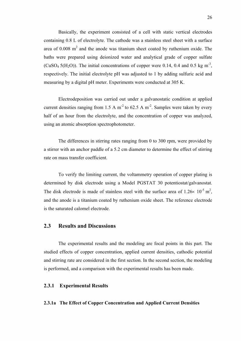
2.2 Normalized copper concentration against time curve

at different applied current densities, with initial concentration

of 0.14 kg m-3, stirring rate 200 rpm..…...………………..…………………27



of 0.4 kg m-3, stirring rate 200 rpm………...……………………………..…27



of 0.5 kg m-3, stirring rate 200 rpm……...…………………………..………28

2.5 A plot of cathodic potential reference saturated calomel

electrode against time at different applied currents,

and initial copper concentration of 0.4 g dm-3……………….……………...29


at different stirring rate,initial copper concentration 0.4 g dm-3

and applied current 0.2 A…………………………………………………....30

2.7 Normalized faradaic current densities against time curve at different

applied current densities, for initial concentration of 0.5 kg m-3,

and stirring rate of 200 rpm ………………………………………………....33

LIST OF FIGURES Figure Page

xvii

2.8 A plot of experimental and predicted normalized

copper concentration evolution versus time at different applied

current densities, initial concentration of 0.14 kg m-3,

and stirring rate of 200 rpm………….…………………..…………………..34


copper concentrations evolution versus time at different applied


and stirring rate of 200 rpm…………………………...……………………..35


copper concentrations evolution versus time at different applied


and stirring rate of 200 rpm……………………………………...…………..35



1.1 Length scales of electrochemical phenomena

entering into theoretical modeling……...……………..……………….……38

1.2 Secondary current distribution in the Hull cell

calculated for different values of Wagner number

assuming Tafel kinetics…………………………….………………………..41

1.3 Standard Hull cell, dimension indicates in mm………………….………….42

1.4 Standard Hull cell theoretical current density

distribution at 2 A total current…………………...…………………………43

1.5 Hydrodynamically Controlled Hull Cell……………………...……………..44

1.6 Hydrodynamically Controlled Hull Cell: (a) HCHC, partially

submerged with one baffle; (b) Equipotential line distribution

calculation; two-dimensional representation of the cell:


xviii

vertical distance from cell bottom;

horizontal distance from cathode surface……..……...…………..…………45

1.7 Rotating disk cathode and stationary cylinder anode..……………………...45

1.8 Deposit thickness distribution on a rotating cone surface..…………………46

1.9 The hydrodynamic electroplating test cell..…………………………………47

1.10 The thickness and current distributions for the Hull cell

and the hydrodynamic electroplating test cell

(HETC) without agitation…………………………………………………...48

1.11 Rotating Cylinder Hull (RCH) cell for electrodeposition studies. ….………48

1.12 The modified Mohler cell with forced electrolyte flow.……………….……49

2.1 Schematic of the Mohler cell.…...…………………………………………..51

2.2 The modified Mohler cell with forced electrolyte flow……………………..52

2.3 Electrolyte circuit…………………………………………………………....52

2.4 Partition of copper deposit

on cathode surface of the Mohler cell…………………...…………………..54

2.5 Dependence of dimensionless current density

distribution versus dimensionless distance

for various average current densities……………..…………………….…...55

2.6 Dependence of the dimensionless current density distribution versus

dimensionless distance for various average current densities,

and comparison with simulated results corresponding to

a primary current distribution……………………………………...………..56

2.7 Dependence of current density distribution versus distance……….………..57

2.8 Potential distribution in the reactor,

(a) our modified Mohler cell and (b) the original Mohler cell……………...58

2.9 Schematic diagram of the conventional RCH cell………….……………….59

2.10 Dimensionless current density (i(x)/iave) represented

as a function of the dimensionless length (x*)……...…….…………………60


xix

2.11 Dimensionless current density (i(x)/iave) represented as a function

of the dimensionless length (x*) and comparison with theoretical

results corresponding to a (1D), (2D) and (3D)………………..……………61

2.12 Variation of dimensionless current density distribution

versus dimensionless distance at various rotating speeds…….….…………..62


1.1 Factors influencing the composition and

structure of electroplated alloys……………………..…………….………...66

1.2 Scheme showing the logarithm of the partial current densities……………..69

1.3 Effect of current density on deposit composition……………...…………....74

1.4 Effect of current density on the percentage of nickel

in Zn-Ni alloys electrodeposited regarding percentages of nickel…………..76

1.5 Effect of current density on the percentage of nickel

in Zn-Ni alloys electrodeposited at various temperatures…..………………76

1.6 Polarization curve during alloy deposition (V/Ag/AgCl) and

effect of current density on nickel content of deposits,

on current efficiency for alloy deposition and on current

efficiency for hydrogen reduction…………………………………..……….77

1.7 Polarization curves for potentiostatic depositions….……………………….78

1.8 Partial current densities for nickel and zinc as

a function of applied potential during Zn-Ni alloy

deposition and pure metal deposition from baths………...………….……...79

1.9 Effect of potential on the percentage of nickel

in zinc nickel alloys electrodeposited………………..………………….…..80

1.10 Polarization curves and nickel percentage

in the deposits obtained at various temperatures…………………..…….….80


xx

1.11 Effect of the nickel percentage in the bath

on the nickel percentage of the deposits

obtained at various potential value…………...……………………..……….81

1.12 Dependence of the Ni content of the alloys

on the deposition time for Zn-Ni deposits

obtained under different conditions………………..………….………..……82

1.13 XPS depth profiles of Zn-Ni alloys at 20 mA cm-2

on commercial iron substrate.…………………………….…………….……83

2.1 General scheme of the EQCM/SIJ setup…………………….…….…………99

2.2 The current ratio of zinc to nickel versus current quantity…………....…….101

2.3 Nickel, zinc and hydrogen currents evolution

versus the deposition time. Eapp = -1.2 V/ SCE. ZnCl2 0.05 mol/L,

NiCl2 6H2O 0.05 mol/L and pH of 4………….……………………………102

2.4 Nickel, zinc and hydrogen currents evolution

versus the deposition time. Eapp = -1.5 V / SCE. ZnCl2 0.05 mol/L,

NiCl2 6H2O 0.05 mol/L and pH of 4……………………………….………104

2.5 Hydrogen evolution on zinc and nickel substrates…………………..…….105

2.6 Nickel deposition on zinc and nickel substrates………………………...…107

2.7 Zinc deposition on zinc and nickel substrates………..…………………....108

2.8 Hydrogen evolution current density for alloy

and elemental experiments data…………………………………………....109

2.9 Nickel current density for alloy and elemental experiments data……….....110

2.10 Zinc current density for alloy and elemental experiment data……………..110

2.11 The influence of coelement concentration

on nickel partial current density………………………………...………….111

2.12 The influence of coelement concentration

on zinc partial current density…………………..………………………….112


xxi

3.1 Diagram of Zn-Ni alloy codeposition ………………………………..…….116

3.2 Scheme of nickel deposition on nickel substrate.…………….…………….123

3.3 The experiment and model simulation of Ni_Ni. ………………………….127

3.4 The experiment and model simulation of H2_ Ni……………………….….127

3.5 Scheme of zinc deposition on zinc substrate……………………………….128

3.6 The experimental and model simulation of Zn_Zn. ………….……………131

3.7 The experimental and model simulation of H2_Zn………...……………....131

3.8 Chronoamperogram of Zn-Ni and Ni_Zn elemental deposition……...……132

3.9 Sketch of the mechanism assumed for nickel deposition

on zinc substrate……………………………………………………………132

3.10 The experimental and model simulation of Ni_Zn. ………………………..135

3.11 The experimental and model simulation of H2_Zn…………………………136

3.12 Sketch of the mechanism assumed for zinc deposition

on nickel substrate…………………………………………………...……..136

3.13 The experimental and model simulation of Zn_Ni…………………………139

3.14 The experimental and model simulation of H2_Ni. ……………..…………140

3.15 Nickel partial current density in alloy simulation

and experimental data (substrate model) .……………...…………………..141

3.16 Zinc partial current density in alloy simulation

and experimental data(substrate model)..…...…………….………….……141

3.17 Hydrogen partial current density in alloy simulation

and experimental data (substrate model) ……………………...…………..142

3.18 Percentage of nickel in alloy simulation and experimental data…...……....142

3.19 Partial current density of zinc in alloy simulation

and experimental data obtained by Trial & Error method…………….……144

3.20 Partial current density of nickel in alloy simulation

and experimental data obtained by Trial & Error method ……….………...144


xxii

3.21 Partial current density of hydrogen in alloy simulation

and experimental data obtained by Trial & Error method ………..………..145

3.22 Percentage of nickel in alloy simulation and experimental

data obtained by Trial & Error method……………………………….…….145

3.23 Predicted influence of coelement concentration

on nickel partial current (substrate model) …………………………..…….146


on zinc partial current (substrate model) ………….……………………….147

3.25 Diagram of Zn-Ni alloy codeposition………………………………………151

3.26 Nickel partial current density in alloy simulation

and experimental data (mixed species model) ……………………………..158

3.27 Zinc partial current density in alloy simulation

and experimental data (mixed species model)…………………….………..158

3.28 Hydrogen evolution partial current density in alloy simulation

and experimental data (mixed species model) ………………………….….159


on nickel partial current (mixed species model) …..…………………….....160


on zinc partial current (mixed species model) …………………………......160

3.31 Effect of KCl complexing agent on the Chronoamperogram…………....…164

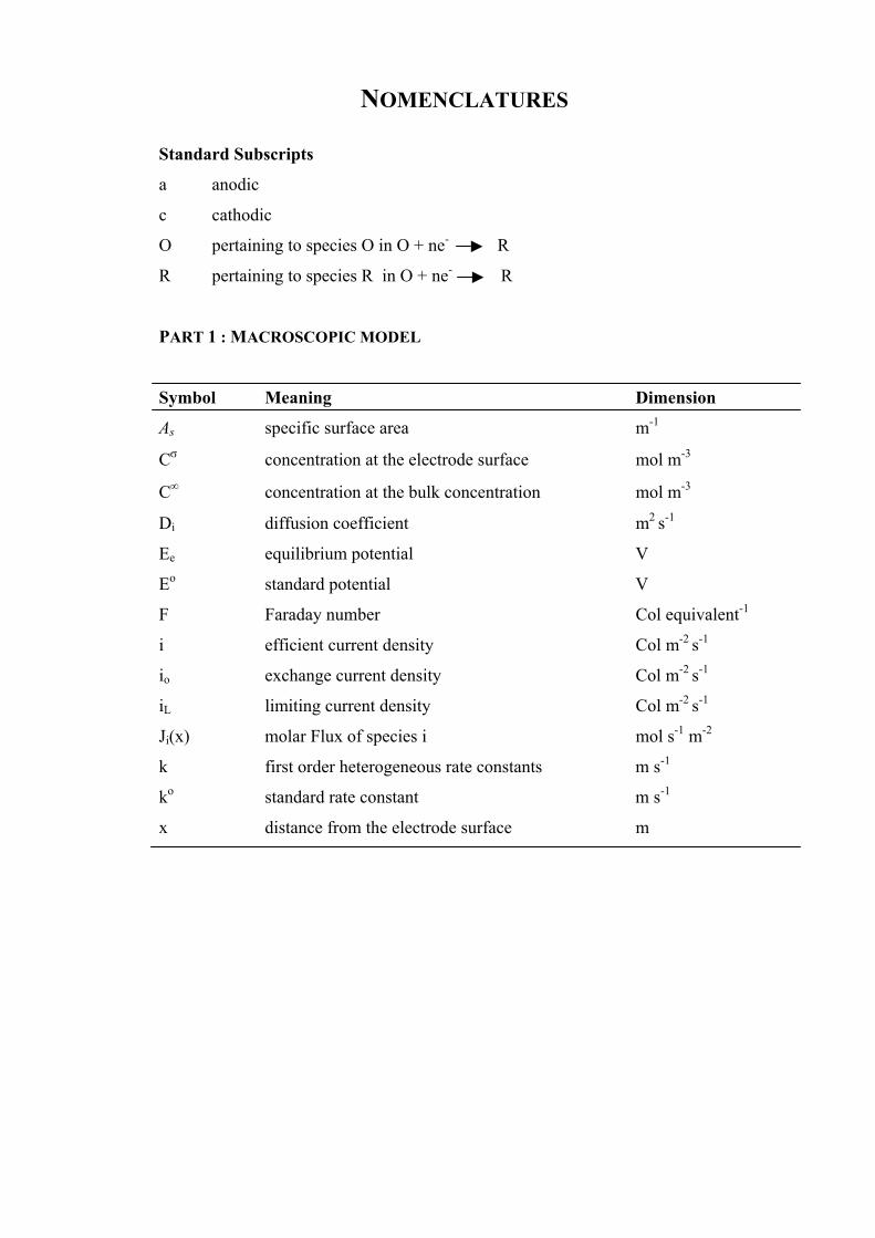
NOMENCLATURES

Standard Subscripts

a anodic

c cathodic

O pertaining to species O in O + ne- R

R pertaining to species R in O + ne- R

PART 1 : MACROSCOPIC MODEL

Symbol Meaning Dimension

As specific surface area m-1

Cσ concentration at the electrode surface mol m-3

C∞ concentration at the bulk concentration mol m-3

Di diffusion coefficient m2 s-1

Ee equilibrium potential V

Eo standard potential V

F Faraday number Col equivalent-1

i efficient current density Col m-2 s-1

io exchange current density Col m-2 s-1

iL limiting current density Col m-2 s-1

Ji(x) molar Flux of species i mol s-1 m-2

k first order heterogeneous rate constants m s-1

ko standard rate constant m s-1

x distance from the electrode surface m

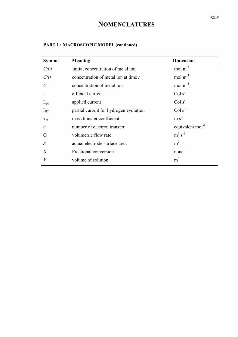
NOMENCLATURES

xxiv

PART 1 : MACROSCOPIC MODEL (continued)


C(0) initial concentration of metal ion mol m-3

C(t) concentration of metal ion at time t mol m-3

C concentration of metal ion mol m-3

I efficient current Col s-1

Iapp applied current Col s-1

IH2 partial current for hydrogen evolution Col s-1

km mass transfer coefficient m s-1

n number of electron transfer equivalent mol-1

Q volumetric flow rate m3 s-1

S actual electrode surface area m2

X Fractional conversion none

V volume of solution m3

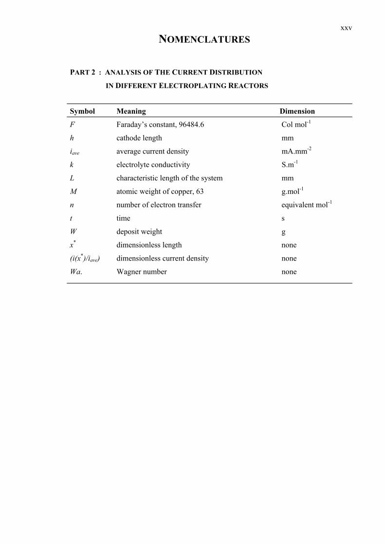
NOMENCLATURES

xxv




F Faraday’s constant, 96484.6 Col mol-1

h cathode length mm

iave average current density mA.mm-2

k electrolyte conductivity S.m-1

L characteristic length of the system mm

M atomic weight of copper, 63 g.mol-1

n number of electron transfer equivalent mol-1

t time s

W deposit weight g

x* dimensionless length none

(i(x*)/iave) dimensionless current density none

Wa. Wagner number none

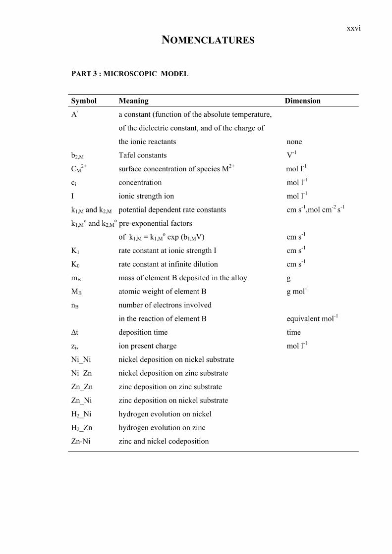
NOMENCLATURES

xxvi



A/ a constant (function of the absolute temperature,

of the dielectric constant, and of the charge of

the ionic reactants none

b2,M Tafel constants V-1

CM2+ surface concentration of species M2+ mol l-1

ci concentration mol l-1

I ionic strength ion mol l-1

k1,M and k2,M potential dependent rate constants cm s-1,mol cm-2 s-1

k1,Mo and k2,M

o pre-exponential factors

of k1,M = k1,Mo exp (b1,MV) cm s-1

K1 rate constant at ionic strength I cm s-1

K0 rate constant at infinite dilution cm s-1

mB mass of element B deposited in the alloy g

MB atomic weight of element B g mol-1

nB number of electrons involved

in the reaction of element B equivalent mol-1

∆t deposition time time

zi, ion present charge mol l-1

Ni_Ni nickel deposition on nickel substrate

Ni_Zn nickel deposition on zinc substrate

Zn_Zn zinc deposition on zinc substrate

Zn_Ni zinc deposition on nickel substrate

H2_Ni hydrogen evolution on nickel

H2_Zn hydrogen evolution on zinc

Zn-Ni zinc and nickel codeposition

NOMENCLATURES

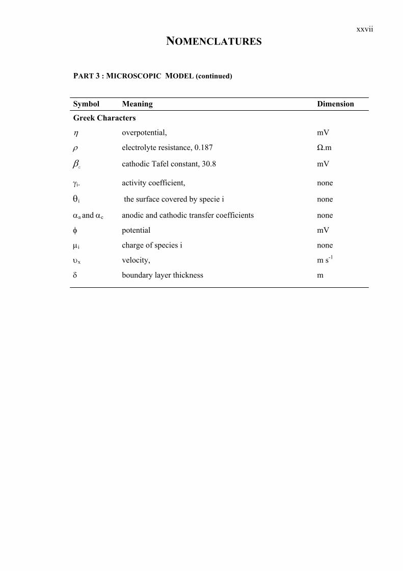
xxvii

PART 3 : MICROSCOPIC MODEL (continued)


Greek Characters

η overpotential, mV

ρ electrolyte resistance, 0.187 Ω.m

βc cathodic Tafel constant, 30.8 mV

γi. activity coefficient, none

θi the surface covered by specie i none

αa and αc anodic and cathodic transfer coefficients none

φ potential mV

µi charge of species i none

υx velocity, m s-1

δ boundary layer thickness m

GENERAL INTRODUCTION

Nowadays, electrochemistry has wide application fields including thin or thick

layer depositions, metals machining, energy production or organic synthesis without

forgetting organic and heavy metals depolluting. For each application, the necessary

knowledge to conduct the process is different and the analysis scale differs also

depending on the needed accuracy.

Over 10 years ago, a lot of studies deal with the electrolytic removal

(electrodeposition, electrocoagulation, electroprecipitation, etc) of heavy metals. By

reason of environmental constraint, it corresponds to an only one step process, which

can provide great economical profits. The operating cost is much cheaper than that of

conventional process and no or little volume of sludge is produced during an

electrochemical process compared with conventional chemical precipitation process.

The strongest advantage of electrochemical process is no chemical contamination in

treated water. In this kind of process the main parameter is the metal concentration. In

this case, a macroscopic model is often sufficient to design and built the apparatus,

which permit to destroy the pollutant. This model can also predict the evolution of the

pollutant species versus time and constitute a convenient tool to operate these

processes.

In recent years, electrochemistry application has been increasingly interested

in the electronics industry, generally micro-industrial applications. The micro-

industrial applications use electrochemical deposition to build layer or device by

electrodeposition of metallic layers. Also, micromachining is used to build holes, and

so on, necessary to elaborate microsystems. In this case, the knowledge of the metal

concentration evolution versus the time is less interesting. It is better to know the

current distribution on the electrode to design a best device, which is able to generate

items required. The metal deposition operations depend on a great number of

chemical and operational parameters such as local current density, electrolyte

concentrations, complexing agents, buffer capacity, pH, leveling agents, brighteners,

surfactants, contaminants, temperature, agitation, substrate properties, cleaning

procedure. All these parameters act on the structure of the deposit and also on its

xxix

composition, in terms of alloy and its properties. Accordingly, the determination of

these parameters is very important. These parameters are often determined

empirically. For this, a lot of experiments have to be studied the effect of the

operating conditions, mainly the applied current density. To decrease this number of

experiments, some cells with specific geometries have been elaborated so as to

produce well-known non-homogeneous distribution. In relation to these cells, it

greatly ease to test a wide range of current density effects, depending on the cell used.

Even if these cells provide an easier and quickest way to develop a new plating

process, they do not give a better understanding of phenomena undergoing in the

reactor. So, it is better to develop a model, which can explain phenomena being used

to conduct their process.

The increasing availability of computing power is able to simulate complex

electrochemical phenomena, which in the past must be studied in a more empirical

and qualitative way. There is a difficulty studying all relevant parameters of

microscopic mathematical models for deposition process. Microscopic models are

nevertheless greatly useful because they quantitatively examine relationships, existing

among mutually dependent parameters. Microscopic mathematical modeling can be

applied to many different deposition problems, for example:

- Identification of mechanisms as a guide to new alloy development

experiments.

- Criteria for process scale up or scale down.

- Cell design and optimization

In the case of alloy deposition, these models could also be used, for example:

- Prediction of the alloy composition from a minimum number of

experiments.

- Control of local composition variations on a nanoscopic, microscopic

or macroscopic scale based on the consideration of current and reaction

distribution.

But these models need parameters, which are easier to determine for a single metal

deposition, comparing with an alloy.

xxx

As mentioned above, all information is summarized and then applied for a

plating process. It appears that:

- Macroscopic models are needed to follow the concentration species

during the plating process in order to know when species must be

added to avoid their depletion or when the bath must be changed. This

model could also be useful to design and conduct an electrochemical

process to destroy cleanly plating bath at its end of life. This fact is

more and more important in plating process due to environmental

constraints.

- Experimental or theoretical determination of the current distribution in

the reactor is necessary to conveniently design the reactor, in order to

obtain layers with the desired properties.

- Determinations of mechanisms and of its parameters are important to

subsequently build models to permit a better understanding of what

happen in the reactor and optimize the process.

Thus, this report is composed of three parts. The first part, dealing with the

macroscopic modelling of the electrochemical reactor, comprises two chapters. The

first one is a bibliographic review including different concepts necessary to introduce

and well understand the different macroscopic models. The second chapter presents

initial experimental results, obtained during the recovery of copper by using a batch

reactor. These results are further compared with those coming from a macroscopic

model.

The second part affects the analysis of the current distribution in different

electroplating reactors. This part is made up of two chapters. The first presents a

bibliographic report concerning different cells that have been built to develop special

current distribution in order to check the effect of the current distribution on the bath

efficiency. In the second chapter, there are experimental results obtained with two

kinds of reactors. These results concern mainly the current distribution in these

devices. These distributions are explained and the efficiency of each cell is

xxxi

commented before presenting a classification of the various cells versus the goal

chosen.

In the last part, the research team concentrates on the proposal of mechanism

models and the determination of the parameter of mathematical models, predicting the

composition of an electrodeposited binary alloy. For this work, the Zn-Ni alloy is

chosen due to this alloy presents an anomalous deposition being difficult to modeling.

Also, it presents an industrial interest for protecting steel against corrosion. This part

consists of three chapters. The first one is a review of the bibliography, regarding

alloy deposition, and more specifically about Zn-Ni alloy deposition. The second

chapter presents a set of experiments being performed in order to check the different

models presented previously and also to be used subsequently for determining the

parameter of models. In the third chapter of this part, it is focused on the modeling of

the Zn-Ni alloy. Two models, assuming homogeneous current distribution and mass

transport rate on the working electrode, have been used. Each model assumption is

first introduced; afterwards, the parameters of the model are calculated with respect to

the experimental results of the previous chapter. At the end of the chapter, we

conclude on the better-suited model.

At the end of this work, the best practice is given to conduct an electroplating

process and more generally all electrochemical process.

PART 1

MACROSCOPIC MODEL

Introduction Plating baths are composed of one or several metals that are used to deposit in

the electrode surface. During the plating process, the metal concentration is decreased

with time. The metal concentration and properties effecting on the product quality

therefore should not be too low to use for plating on the substrate material. In this part

we consider the macroscopic model monitoring the bulk concentration of the metal in

the electroplating bath. This study could also be used during the treatment of the

plating bath at the end of its life and electrosynthesis.

Rate of metal deposition could be under two controlled systems, the kinetic

and mass transfer. We study a changing rate of metal concentration by considering

copper concentration versus time. According to this study, we can observe time of

which copper concentration is too low for plating bath. At this time, the bath must be

destroyed before laundry or to be regenerated by adding reacting species. Time

duration for plating process at its end of life can thus be determined.

This macroscopic model section is composed of two chapters; i.e.,

bibliography and experimental parts (monitoring rate of copper concentration). In the

bibliography part, a summary of electrochemistry considering the kinetic and mass

transfer system and the electrochemical reactor has been described. In the

experimental part, the removal rate of copper is monitored versus time under kinetic

and mass transfer controlled.

2

Chapter 1

Bibliography

1.1 Summary of Electrochemical Theory

Electrochemistry involves chemical phenomena associated with a charge

transfer, which can heterogeneously occur on electrode surfaces. In this chapter, a

brief overview of electrochemistry, particularly of electrode reactions are described in

order to show the interdisciplinary nature and versatility of electrochemistry and to

introduce a few of the important fundamental concepts. Before discussing, it is worth

looking briefly at the nature of electrode reactions1.

1.1.1 The Nature of Electrode Reactions

Electrode reactions are heterogeneous and take place in the interfacial region

between electrode and solution. The simplest electrode reaction could inter-convert at

an inert surface, two species, O and R, which are completely stable and soluble in the

electrolysis medium containing an excess of an electrolyte:

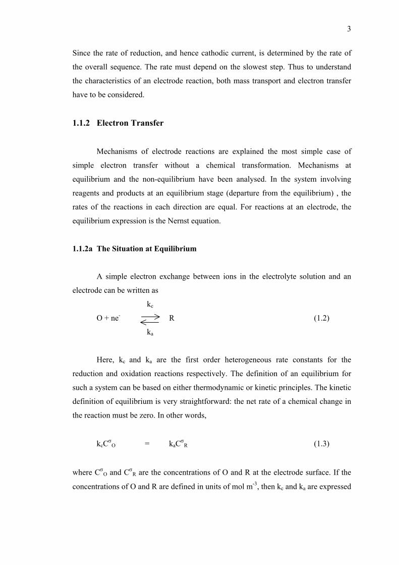
On+ + ne- R (1.1)

The electrode reaction is a sequence of more basic steps. To maintain a current it is

essential to supply reactant to the electrode surface and also to remove the product, as

well as for the electron transfer reaction at the surface to occur. For example, in

experimental conditions where O is reduced to R, the electrode reaction must have

three steps:

Obulk Oelectrode [mass transfer]

Oelectrode Relectrode [charge transfer]

Relectrode Rbulk [mass transfer]

3

Since the rate of reduction, and hence cathodic current, is determined by the rate of

the overall sequence. The rate must depend on the slowest step. Thus to understand

the characteristics of an electrode reaction, both mass transport and electron transfer

have to be considered.

1.1.2 Electron Transfer

Mechanisms of electrode reactions are explained the most simple case of

simple electron transfer without a chemical transformation. Mechanisms at

equilibrium and the non-equilibrium have been analysed. In the system involving

reagents and products at an equilibrium stage (departure from the equilibrium) , the

rates of the reactions in each direction are equal. For reactions at an electrode, the

equilibrium expression is the Nernst equation.

1.1.2a The Situation at Equilibrium

A simple electron exchange between ions in the electrolyte solution and an

electrode can be written as

kc

O + ne- R (1.2)

ka

Here, kc and ka are the first order heterogeneous rate constants for the

reduction and oxidation reactions respectively. The definition of an equilibrium for

such a system can be based on either thermodynamic or kinetic principles. The kinetic

definition of equilibrium is very straightforward: the net rate of a chemical change in

the reaction must be zero. In other words,

kcCσO = kaCσ

R (1.3)

where CσO and Cσ

R are the concentrations of O and R at the electrode surface. If the

concentrations of O and R are defined in units of mol m-3, then kc and ka are expressed

4

in units of m s-1. Alternatively, equilibrium can be defined in terms of the current

densities by the identity

i = ic + ia = 0 (1.4)

where

ic = -nF kcCσO (1.5)

and

ia = nF kaCσR (1.6)

ia for the current of oxidation process has a positive, sign whereas, ic, the current for

the reduction process has a negative sign. ia is referred to as the anodic partial current

density and ic as the cahtodic partial current density. The measured current density, i

(Col m-2 s-1), is therefore made up from contributions of the anodic and cathodic

processes.

Here the key assumption concerns the potential dependence of kc and ka in the

relation 1.2. This is usually written as

−

−=RT

)EnF(Eexpkk ecαocc (1.7a)

and

−

−=RT

)EnF(Eexpkk eaαoaa (1.7b)

where ko is the standard rate constant, and αa and αc are the anodic and cathodic

transfer coefficients, respectively. For the moment, αa and αc are assumed to be

constants which take values between 0 and 1, and it is commonly assumed that

αc = 0.5. Ee (V) is the equilibrium potential related to the standard potential of the

couple O/R, Eo (V).

5

At the equilibrium potential, the anodic and cathodic currents must sum up to

zero, Eq.1.4, the magnitudes of the anodic and cathodic partial currents are identical

to the exchange current density, io:

|ic| = |ia| = io at E = Ee (1.8)

The expression for ic and ia can now be substituted from Eqs. 1.5 and 1.7,

assuming αa = 1 - αc , to give

−−

=

−−

RT)E)nF(E(1

expknFCRT

)EnF(EexpknFC ecαoσ

Recαoσ

o (1.9)

Rearrangement of Eq. 1.9 leads to the expression

σ

σ

R

Ooe C

ClnnFRT+E=E (1.10)

The system is at equilibrium so Cσo = C∞

o and CσR = C∞

R , where C∞o and C∞

R are the

bulk concentration of O and R. Equation 1.10 becomes identical to the Nernst

equation2.

1.1.2b Departure from Equilibrium (Activation Polarization)

It is an experimental fact that the rate of an electron transfer reaction is

sensitive to changes in electrode potential, and it is therefore suitable to choose the

equilibrium potential as a reference point and then to determine the overpotential, η

(V) as.

η = E - Ee (1.11)

6

Alternatively, the overpotential can be referred to the standard potential using the

Nernst equation.

)CCln(

nFRTEE

R

oe ∞

∞

−−=η (1.12)

The exchange current density, io can now be obtained by substitution of Eq.1.12 into

1.9

c1o

cR

oaco )(C)(CnFkiii αα −∞∞=== (1.13)

The net current density can now be expressed in terms of the exchange current density

in the form

−−

−=+= )

RTnFexp()

RT)nF(1exp(iiii cc

ocaηαηα

(1.14)

Eq 1.14 is known as the Butler-Volmer equation2, and it forms the basis for the

theoretical description of electrode processes.

It is often convenient to consider the limiting behavior of Eq 1.14 for small

and large values of the exponential terms. The exponential terms can be written as

Taylor expansions.

For small values of the arguments of the parameters αcnFη / RT and

(1-αc)nFη / RT, the first two terms can be combined into

RTnFi

iηo= for αcnFη/RT << 1 (1.15)

In practice, the linear approximation can be used for |η| << 10/n mV when the error

due to the approximation is about 1% for αc = 0.5.

7

For large positive or large negative overpotentials, under these conditions, one

or other of the exponential terms in the Butler-Volmer equation dominates, the

relation and the limiting relationships become

i = ic = -ioexp(-αcnFη/RT) (1.16a)

for large negative overpotentials, and

i = ia = -ioexp(1-αc)nFη/RT (1.16b)

for large positive overpotentials.

These relationships are often written in the form of the Tafel equations1:

occ

loginF

2.3RTilognF

2.3RTαα

η +−= (η < 0) (1.17a)

oaa

loginF

2.3RTilognF

2.3RTαα

η += (η > 0) (1.17b)

where i is the net current density. The Tafel approximation is generally used for |η| >>

70/n mV.

Eqs. 1.17a and b are known as the Tafel equations and are the basis of a

simple method of determining the exchange current density and a transfer coefficient,

as shown in Figure 1.1.

8

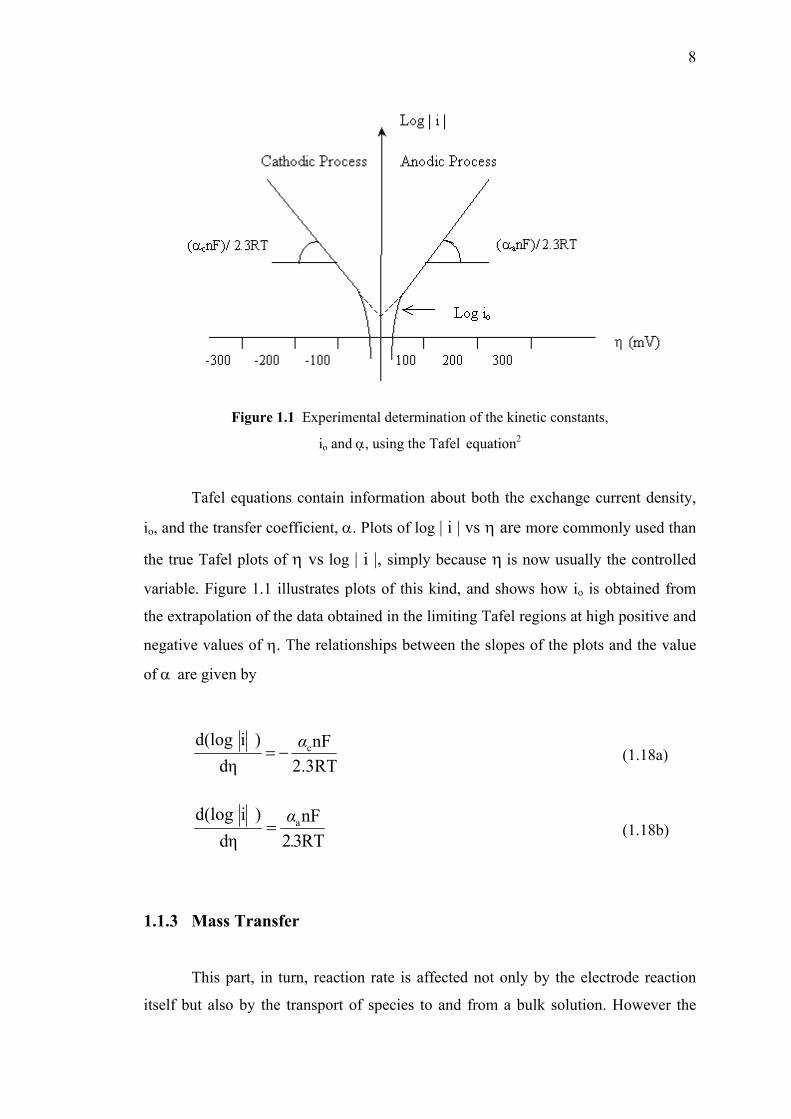
Figure 1.1 Experimental determination of the kinetic constants,

io and α, using the Tafel equation2

Tafel equations contain information about both the exchange current density,

io, and the transfer coefficient, α. Plots of log | i | vs η are more commonly used than

the true Tafel plots of η vs log | i |, simply because η is now usually the controlled

variable. Figure 1.1 illustrates plots of this kind, and shows how io is obtained from

the extrapolation of the data obtained in the limiting Tafel regions at high positive and

negative values of η. The relationships between the slopes of the plots and the value

of α are given by

2.3RTnF

ηd) i d(log cα−= (1.18a)

RT32nF

ηd) i d(log a

.α

= (1.18b)

1.1.3 Mass Transfer

This part, in turn, reaction rate is affected not only by the electrode reaction

itself but also by the transport of species to and from a bulk solution. However the

9

kinetic of electron transfer rate is very rapid compared to mass transfer processes rate.

This mass transport can occur by diffusion, convection, or migration.

Mass transfer is the movement of materials from one location in solution to

another, arises either from differences in electrical or chemical potential at the two

locations. The modes of mass transfer are

1. Migration. Movement of a charged body under the influence of an electric

field (a gradient of electrical potential)

2. Diffusion. Movement of a species under the influence of a gradient of

chemical potential (activities) (i.e., a concentration gradient).

3. Convection. (Stirring or hydrodynamic transport) Generally, fluid flow occurs

because of forced convection, and may be characterized by stagnant regions,

laminar flow, and turbulent flow and natural convection (convection caused by

density gradients),

Mass transfer to an electrode is governed by the Nernst-Planck equation3,

which is written for one-dimensional mass transfer along the x-axis as

(x)Cx(x)C

x(x)CD(x)J xυi

φiiµi

ii +−−=∂

∂

∂

∂ (1.19)

where Ji(x) is the flux of species i (mole s-1 m-2) at distance x from the surface, Di is

the diffusion coefficient (m2 s-1), ∂Ci(x)/ ∂x is the concentration gradient at distance x,

∂φ(x)/ ∂x is the potential gradient, µi and Ci are charge and concentration of species i,

respectively, and υx(x) is the velocity (m s-1) with which a volume element in solution

moves along the axis. The three terms on the right hand side of the equation 1.19

represent the contributions of diffusion, migration, and convection, respectively, to

the flux.

1.1.3a Steady-State Mass Transfer

In the presence of a base electrolyte, diffusion is the only form of mass transport

10

for the electroactive species, which need to be considered. The simplest model is that

of linear diffusion to a plane electrode; it is assumed that the electrode is perfectly flat

and of infinite dimensions, so that concentration variables can only occur

perpendicular to the electrode surface. Diffusion may then be characterized by Fick ’s

law in a one dimensional form.

Fick ’s law states that the flux of any species, i, through a plane parallel to the

electrode surface is given by

dxdCD)x(J i

ii −= (1.20)

where Di is the diffusion coefficient and typically has values around 10-9 m2 s-1.

The number of electron reaching to the current is constant versus time,

i = -d (ne-) /dt. The first law applied at the electrode surface, x = 0, is used to relate

the current to the chemical change at the electrode by equating the flux of O or R with

the flux of electrons, where

0x

Oc x

CDnFi

=∂

∂

−= (1.21a)

or

0x

Ra x

CDnFi

=∂

∂

= (1.21b)

Close to the electrode surface zone, convection will not be an important form

of mass transport, and it is therefore possible and certainly convenient for

understanding of a boundary layer thickness, δ, which diffusion is the only significant

form of mass transport. Outside this boundary layer, convection is strong enough to

maintain the concentrations of all species uniform and at their bulk values. Using this

11

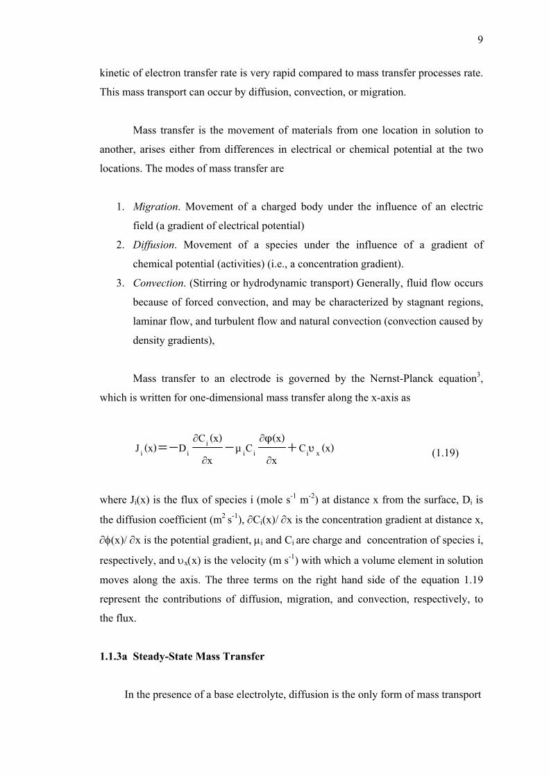
concept, the steady state concentration profiles for a solution of O and R are shown in

Figure 1.2.

Figure 1.2 Steady-state concentration profiles for the process O + ne- R 2

With the rotating disc electrode, the diffusion later thickness is determined by the

rotation rate of the disc, the layer becoming thinner with increasing rotation rate. The

Ci vs x plot inside the boundary layer must, in the steady state, be effectively linear.

The steady state will be given by

δo

σo

0x

o∞

=

−=

−=

CCnFDdx

dCnFDi (1.22)

The surface concentration Cσο is, of course, a function of potential, but the diffusion

limited current density or limiting current density, iL corresponds to the maximum

flux, i.e. to potentials where Cσο = 0.3 Therefore

δ

∞

= oL

nFDC-i (1.23)

From equations 1.22 and 1.23, it could be deduced to

Lii

CC

−=∞ 1

o

σo

(1.24)

12

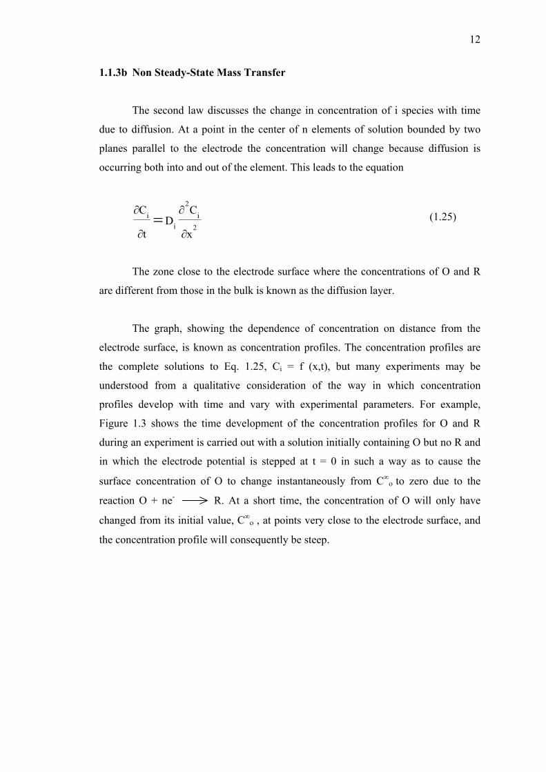
1.1.3b Non Steady-State Mass Transfer

The second law discusses the change in concentration of i species with time

due to diffusion. At a point in the center of n elements of solution bounded by two

planes parallel to the electrode the concentration will change because diffusion is

occurring both into and out of the element. This leads to the equation

2

2

xCD

tC i

ii

∂

∂

∂

∂= (1.25)

The zone close to the electrode surface where the concentrations of O and R

are different from those in the bulk is known as the diffusion layer.

The graph, showing the dependence of concentration on distance from the

electrode surface, is known as concentration profiles. The concentration profiles are

the complete solutions to Eq. 1.25, Ci = f (x,t), but many experiments may be

understood from a qualitative consideration of the way in which concentration

profiles develop with time and vary with experimental parameters. For example,

Figure 1.3 shows the time development of the concentration profiles for O and R

during an experiment is carried out with a solution initially containing O but no R and

in which the electrode potential is stepped at t = 0 in such a way as to cause the

surface concentration of O to change instantaneously from C∞ο to zero due to the

reaction O + ne- R. At a short time, the concentration of O will only have

changed from its initial value, C∞ο , at points very close to the electrode surface, and

the concentration profile will consequently be steep.

13

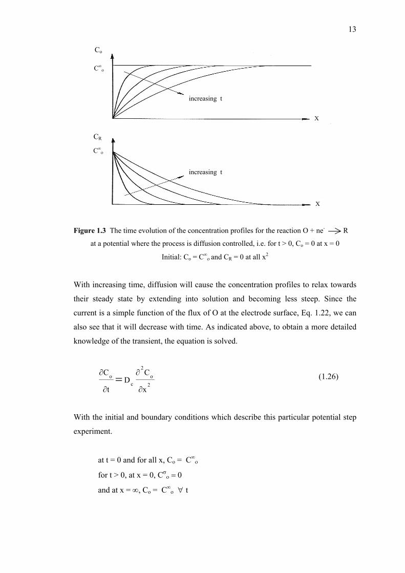
Figure 1.3 The time evolution of the concentration profiles for the reaction O + ne- R

at a potential where the process is diffusion controlled, i.e. for t > 0, Co = 0 at x = 0

Initial: Co = C∞ο and CR = 0 at all x2

With increasing time, diffusion will cause the concentration profiles to relax towards

their steady state by extending into solution and becoming less steep. Since the

current is a simple function of the flux of O at the electrode surface, Eq. 1.22, we can

also see that it will decrease with time. As indicated above, to obtain a more detailed

knowledge of the transient, the equation is solved.

2

2

xCD

tC o

co

∂

∂

∂

∂= (1.26)

With the initial and boundary conditions which describe this particular potential step

experiment.

at t = 0 and for all x, Co = C∞ο

for t > 0, at x = 0, Cσο = 0

and at x = ∞, Co = C∞ο ∀ t

C∞ο

C∞ο

Co

CR

increasing t

increasing t

X

X

14

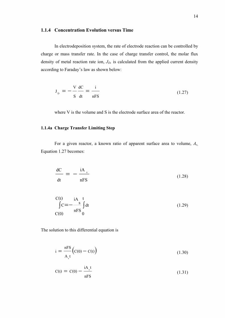
1.1.4 Concentration Evolution versus Time

In electrodeposition system, the rate of electrode reaction can be controlled by

charge or mass transfer rate. In the case of charge transfer control, the molar flux

density of metal reaction rate ion, JD, is calculated from the applied current density

according to Faraday’s law as shown below:

nFSi

dtdC

SVJ D =−= (1.27)

where V is the volume and S is the electrode surface area of the reactor.

1.1.4a Charge Transfer Limiting Step

For a given reactor, a known ratio of apparent surface area to volume, As,

Equation 1.27 becomes:

nFSiA

dtdC s−= (1.28)

∫−=∫t

0dt

nFSsiAC(t)

C(0)C (1.29)

The solution to this differential equation is

( )C(t)C(0)tA

nFSis

−= (1.30)

nFStiAC(0)C(t) s−= (1.31)

15

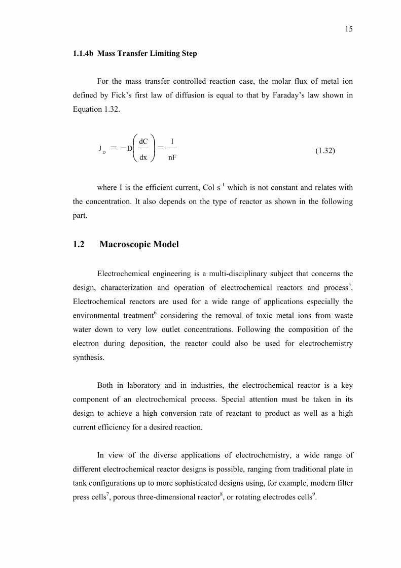
1.1.4b Mass Transfer Limiting Step

For the mass transfer controlled reaction case, the molar flux of metal ion

defined by Fick’s first law of diffusion is equal to that by Faraday’s law shown in

Equation 1.32.

nFI

dxdCDJ D =

−= (1.32)

where I is the efficient current, Col s-1 which is not constant and relates with

the concentration. It also depends on the type of reactor as shown in the following

part.

1.2 Macroscopic Model

Electrochemical engineering is a multi-disciplinary subject that concerns the

design, characterization and operation of electrochemical reactors and process5.

Electrochemical reactors are used for a wide range of applications especially the

environmental treatment6 considering the removal of toxic metal ions from waste

water down to very low outlet concentrations. Following the composition of the

electron during deposition, the reactor could also be used for electrochemistry

synthesis.

Both in laboratory and in industries, the electrochemical reactor is a key

component of an electrochemical process. Special attention must be taken in its

design to achieve a high conversion rate of reactant to product as well as a high

current efficiency for a desired reaction.

In view of the diverse applications of electrochemistry, a wide range of

different electrochemical reactor designs is possible, ranging from traditional plate in

tank configurations up to more sophisticated designs using, for example, modern filter

press cells7, porous three-dimensional reactor8, or rotating electrodes cells9.

16

In this part, the studies focus on an electrochemical reactor that is an

established unit process for the pollution control application, i.e., removing heavy

metal in wastewater stream. The operation under charge transfer and mass transfer

controlled has been analyzed, taking into account the idealized batch reactor and

flow-through reactors in the single pass mode.

Two types of ideal fluid flow through the reactor, namely plug flow and

perfect mixing flow, are commonly considered. In the first case, it is assumed that the

fluid flow is continuous through the reactor with no mixing of the electrolyte in the

direction of the flow between inlet and outlet, under steady state mode. The reactant

and product concentrations are both functions of the distance but they are independent

of time. As a result, the residence time must be equal for all species in the reactor. A

reactor with such properties is called a plug flow reactor (PFR).

A perfectly stirred tank with a continuous flow through the reactor is called a

continuously stirred tank reactor (CSTR). In this case, the concentration of reactants

and products are uniform throughout the reactor. The reactant concentration within

the reactor is equal to the outlet concentration, C(OUT), and is independent of time.

The most common example of a perfectly mixed reactor is the simple batch

reactor in which the reactant is continuously stirred throughout a batch time during

which reaction occurs. During the batch processing time, the concentration of

reactants and products will progressively change. At any instant, however, the

electrolyte composition is uniform through the reactor. The batch reactor is widely

used due to its simplicity and versatility. Batch reactors are used for small-scale

operations where they are more economical than continuous reactors. Figure 1.4

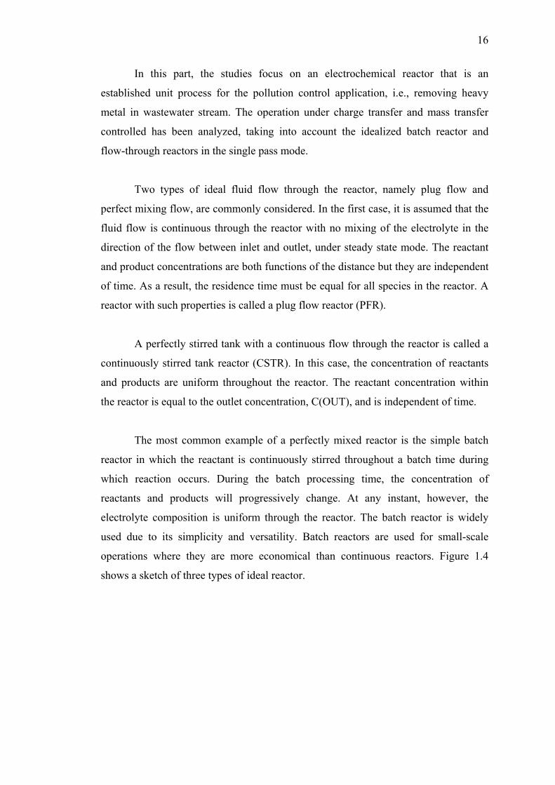
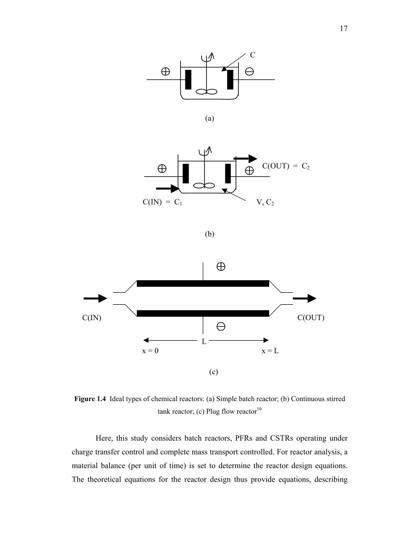
shows a sketch of three types of ideal reactor.

17

(a)

(b)

(c)

Figure 1.4 Ideal types of chemical reactors: (a) Simple batch reactor; (b) Continuous stirred

tank reactor; (c) Plug flow reactor10

Here, this study considers batch reactors, PFRs and CSTRs operating under

charge transfer control and complete mass transport controlled. For reactor analysis, a

material balance (per unit of time) is set to determine the reactor design equations.

The theoretical equations for the reactor design thus provide equations, describing

C

V, C2

C(OUT) = C2

C(IN) = C1

C(IN) C(OUT)

L x = 0 x = L

18

reactor’s performance in terms of conversion and as a function of the mass transport

coefficient, km.

1.2.1 Kinetic and Mass Transport in the Electrochemical Reactor

The conversion of an oxidized (Ox) to a reduced (Re) species of a redox

couple Ox/Re can be considered:

O + ne- R (1.33)

The material balance is based on the principle of the matter conservation. In

the case of the component O in reaction 1.33, this material balance can be written as:

Rate of mass input = Rate of mass output + Rate of loss (1.34)

- For the case of a batch reactor, there is no inputs and outputs, so the

relationship of Eg. 1.34 can be simplified to:

Rate of accumulation of O = - Rate of disappearance of O (1.35)

- For the case of PFR and CSTR, there is no accumulation and the

material balance for component O can be written as:

Rate of mass input - Rate of mass output = Rate of mass disappearance (1.36)

In an electrochemical reaction the rate of mass disappearance of Ox (i.e.,

d[O]/dt) is given by the expression:

I /nFV = -d[O] /dt (1.37)

where I is the cell current (A) , n is the number of electrons involved in the electrode

reaction and F is the Faraday constant (mole ). [O] is the concentration of component

19

O (mole m-3) and V is volume of the electrolyte (m-3). The quantity I = nF is the rate

of reaction and has units of mol s-1.

Here, the reaction is considered to take place under mass transport control and

the value of I is the limiting current, Il (Col s-1) is given by:

Il = nFkm ACB (1.38)

where km is the mass transport coefficient which unit cm s-1 (a type of heterogeneous

rate constant), A is the electrode area (m2) and CB is the concentration of the

electroactive species in the bulk electrolyte (mole m-3).

Bard and Faulkner3 have described the characteristic of controlled current

electrolysis, the change of the limiting current with time.

As long as the applied current (Iapp) is less than the limiting current (Il) at a

given bulk concentration, the electrode reaction proceeds with 100% current

efficiency. As the electrolysis proceeds, the bulk concentration of metal ion decreases

with time and the limiting current decreases linearly with time.

At longer time, magnitude of the applied current is more than that of the

limiting current, and the potential shifts to more negative value, where an additional

electrode reaction can occur. This reaction contributes to the additional current, Iapp –

Il = IH2. The current efficiency thus drops below 100%.

It is useful to express reactor performance in terms of the fractional reactant

conversion, X. In the case of a constant volume system, this may be defined as10.

X = (Co - C) / Co (1.39)

where Co (mole cm-3) is the initial concentration of reactant and C (mole cm-3) is the

concentration at t time. 0<X<1, X=0 for t = 0 and X 1 for t ∞

20

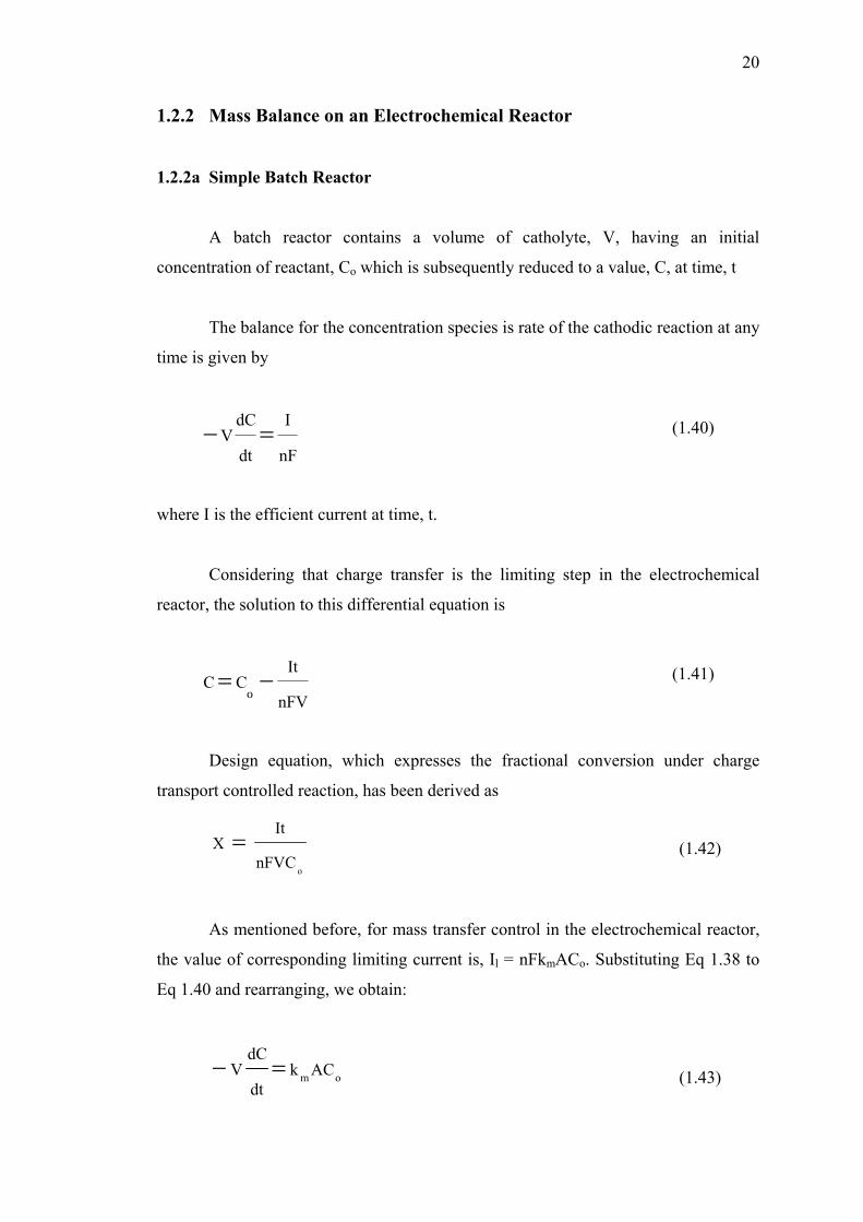
1.2.2 Mass Balance on an Electrochemical Reactor

1.2.2a Simple Batch Reactor

A batch reactor contains a volume of catholyte, V, having an initial

concentration of reactant, Co which is subsequently reduced to a value, C, at time, t

The balance for the concentration species is rate of the cathodic reaction at any

time is given by

nFI

dtdCV =− (1.40)

where I is the efficient current at time, t.

Considering that charge transfer is the limiting step in the electrochemical

reactor, the solution to this differential equation is

nFVItCC

ο−= (1.41)

Design equation, which expresses the fractional conversion under charge

transport controlled reaction, has been derived as

onFVCItX = (1.42)

As mentioned before, for mass transfer control in the electrochemical reactor,

the value of corresponding limiting current is, Il = nFkmACo. Substituting Eq 1.38 to

Eq 1.40 and rearranging, we obtain:

om ACkdtdCV =− (1.43)

21

C = Co exp(-kmAt / V ) (1.44)

Design equation, which expresses the fractional conversion under mass


X = 1-exp(-kmAt / V ) (1.45)

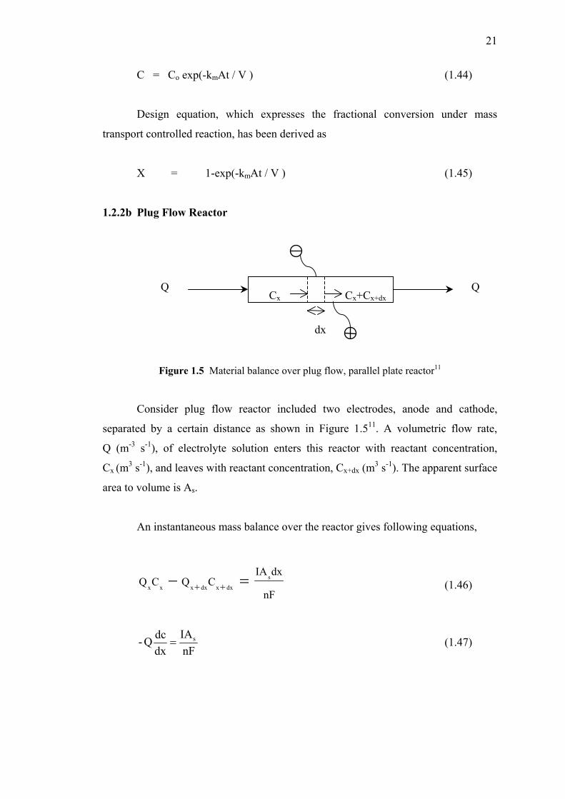
1.2.2b Plug Flow Reactor

Figure 1.5 Material balance over plug flow, parallel plate reactor11

Consider plug flow reactor included two electrodes, anode and cathode,

separated by a certain distance as shown in Figure 1.511. A volumetric flow rate,

Q (m-3 s-1), of electrolyte solution enters this reactor with reactant concentration,

Cx (m3 s-1), and leaves with reactant concentration, Cx+dx (m3 s-1). The apparent surface

area to volume is As.

An instantaneous mass balance over the reactor gives following equations,

nFdxIACQCQ s

dxxdxxxx =− ++ (1.46)

nFIA

dxdcQ- s= (1.47)

Cx Cx+Cx+dx Q

dx

Q

22

dxQnFIAdC s−= (1.48)

Considering that charge transfer is the limiting step in the electrochemical

reactor, the solution to this differential equation is

xQnFIACC s

o −= (1.49)

Design equation, which expresses the fractional conversion under charge transport

controlled reaction, has been derived as

xQnFC

IAXo

s= (1.50)

As mentioned before, for mass transfer control in the electrochemical reactor,

the value of corresponding limiting current is, Il = nFkmACo. Substituting Eq 1.38 to

Eq 1.48 and rearranging, we obtain

QCAk

dxdC sm=− (1.51)

dxQCAk

CdC sm=− (1.52)

)Q

xAkexp(CC smo −= (1.53)

Design equation which expresses the fractional conversion under mass transport

controlled reaction, has been derived as

23

)Q

xAkexp(1X sm−−= (1.54)

1.2.2c Continuous Stirred Tank Reactor

Considering the CSTR when the device consists of a single compartment as

seen in Figure 1.4b. The flow rates of solution, entering and leaving the reactor, are

equal to Q (m3 s-1). The terminal concentrations of the reacting species being

considered are constant and equal to C1 and C2 (mole cm-3), with a net volume of

V(cm3).

The overall material balance for the general case of a stirred tank reactor, over

a time interval, dt, can be seen from equation11.

nFI)CQ(C 21 =− (1.55)

Under charge transfer control, the solution of the differential equation is

nFQICC 12 −= (1.56)

Design equation which expresses the fractional conversion under charge


1nFQCIX = (1.57)

For a single component CSTR, with the specified reactant undergoing a fast

reaction, the limiting current density is related to the outlet concentration by

IL = nFkm AC2, and Eq 1.52 modifies to

24

(1.58)

Where A represents the electrode area (m2). The terminal concentration is related to

the entrance concentration by

A/Qk1C

Cm

12 +

= (1.59)

which could be compared for the plug flow reactor

The fractional conversion over the reactor under mass transfer control can be

obtained by a simple manipulation on Eq 1.56

A/Qk1A/QkX

m

m

+= (1.60)

Comparing to Eq 1.51, it is evident that a smaller X is obtained with the CSTR than

plug flow reactor for given values of km, A and Q.

1.3 Conclusion

According to literature review, equations for macroscopic models have been

established. Studying the macroscopic models, the experiment should be performed

by considering only the bulk metal concentration evolution versus time. In this case,

charge or mass transfer could control the rate of bulk metal concentration variation.

In order to simplify the model, the batch reactor is used to be the case study. In

addition, copper solution can be used for this experimental determination of current

distributions in a particular reactor. Copper deposition from a sulfate/sulfuric medium

is a well–known electrochemical reaction and can be considered as a test reaction 12.

ACk)CQ(C 2m21 =−

25

Chapter 2

Analyzing Kinetics and Mass Transport

on an Electrochemical Batch Reactor

2.1 Introduction

Kinetic and mass transport of the copper ion reaction rate is studied in this

chapter. The considered parameters are the applied current, initial concentration,

cathodic potential and stirring rate. According to those studied parameters, the

concentrations of copper reducing with time are monitored under the kinetic and mass

transport controlled. A simple batch reactor under galvanostatic conditions is studied

in these experiments. The results, provided by the theoretical macroscopic model, are

compared to the experimental results in the second part of this chapter.

Regarding the idea of plating process, this study helps towards better

understanding a relationship between the decrease of metal ion concentration and

time, with respect to a reduction reaction. Essentially, it leads to identify duration of

depositing process when the metal concentration appears too low. The results

significantly ease our decision to add more reactant species or to terminate the bath.

The time recovery to destroy plating bath at its end of life could also be determined.

2.2 Experiment

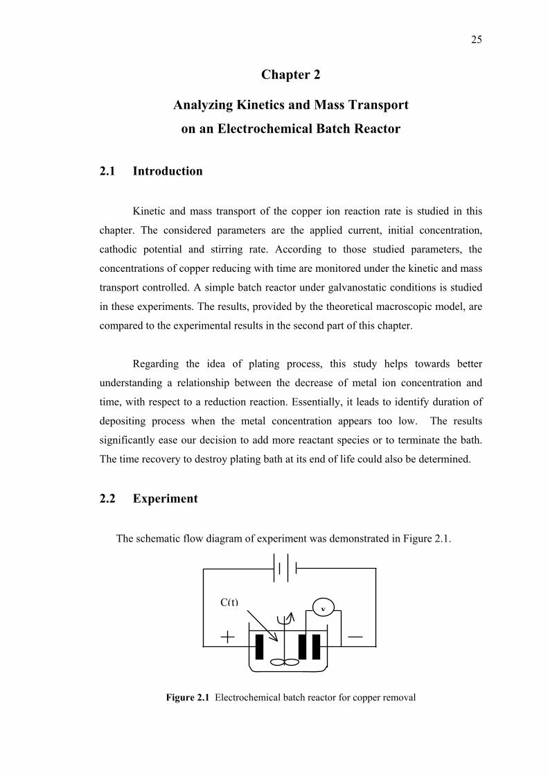
The schematic flow diagram of experiment was demonstrated in Figure 2.1.

Figure 2.1 Electrochemical batch reactor for copper removal

vC(t)

26

Basically, the experiment consisted of a cell with static vertical electrodes

containing 0.8 L of electrolyte. The cathode was a stainless steel sheet with a surface

area of 0.008 m2 and the anode was titanium sheet coated by ruthenium oxide. The

baths were prepared using deionized water and analytical grade of copper sulfate

(CuSO4 5(H2O)). The initial concentrations of copper were 0.14, 0.4 and 0.5 kg m-3,

respectively. The initial electrolyte pH was adjusted to 1 by adding sulfuric acid and

measuring by a digital pH meter. Experiments were conducted at 305 K.

Electrodeposition was carried out under a galvanostatic condition at applied

current densities ranging from 1.5 A m-2 to 62.5 A m-2. Samples were taken by every

half of an hour from the electrolyte, and the concentration of copper was analyzed,

using an atomic absorption spectrophotometer.

The differences in stirring rates ranging from 0 to 300 rpm, were provided by

a stirrer with an anchor paddle of a 5.2 cm diameter to determine the effect of stirring

rate on mass transfer coefficient.

To verify the limiting current, the voltammetry operation of copper plating is

determined by disk electrode using a Model PGSTAT 30 potentiostat/galvanostat.

The disk electrode is made of stainless steel with the surface area of 1.26× 10-5 m2,

and the anode is a titanium coated by ruthenium oxide sheet. The reference electrode

is the saturated calomel electrode.

2.3 Results and Discussions

The experimental results and the modeling are focal points in this part. The

studied effects of copper concentration, applied current densities, cathodic potential

and stirring rate are considered in the first section. In the second section, the modeling

is performed, and a comparison with the experimental results has been made.

2.3.1 Experimental Results

2.3.1a The Effect of Copper Concentration and Applied Current Densities

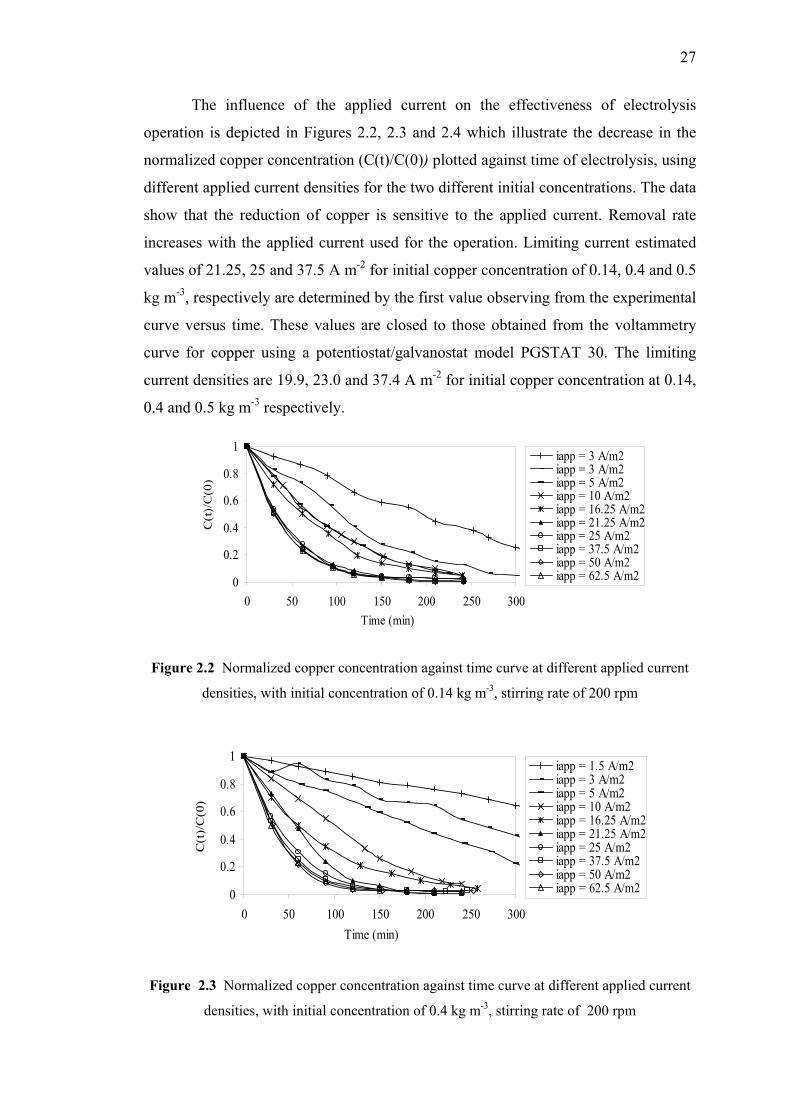
27

The influence of the applied current on the effectiveness of electrolysis

operation is depicted in Figures 2.2, 2.3 and 2.4 which illustrate the decrease in the

normalized copper concentration (C(t)/C(0)) plotted against time of electrolysis, using

different applied current densities for the two different initial concentrations. The data

show that the reduction of copper is sensitive to the applied current. Removal rate

increases with the applied current used for the operation. Limiting current estimated

values of 21.25, 25 and 37.5 A m-2 for initial copper concentration of 0.14, 0.4 and 0.5

kg m-3, respectively are determined by the first value observing from the experimental

curve versus time. These values are closed to those obtained from the voltammetry

curve for copper using a potentiostat/galvanostat model PGSTAT 30. The limiting

current densities are 19.9, 23.0 and 37.4 A m-2 for initial copper concentration at 0.14,

0.4 and 0.5 kg m-3 respectively.

0

0.2

0.4

0.6

0.8

1

0 50 100 150 200 250 300Time (min)

C(t

)/C

(0)

iapp = 3 A/m2iapp = 3 A/m2iapp = 5 A/m2iapp = 10 A/m2iapp = 16.25 A/m2iapp = 21.25 A/m2iapp = 25 A/m2iapp = 37.5 A/m2iapp = 50 A/m2 iapp = 62.5 A/m2

Figure 2.2 Normalized copper concentration against time curve at different applied current

densities, with initial concentration of 0.14 kg m-3, stirring rate of 200 rpm

0

0.2

0.4

0.6

0.8

1

0 50 100 150 200 250 300Time (min)

C(t

)/C

(0)

iapp = 1.5 A/m2iapp = 3 A/m2iapp = 5 A/m2iapp = 10 A/m2iapp = 16.25 A/m2iapp = 21.25 A/m2iapp = 25 A/m2iapp = 37.5 A/m2iapp = 50 A/m2iapp = 62.5 A/m2



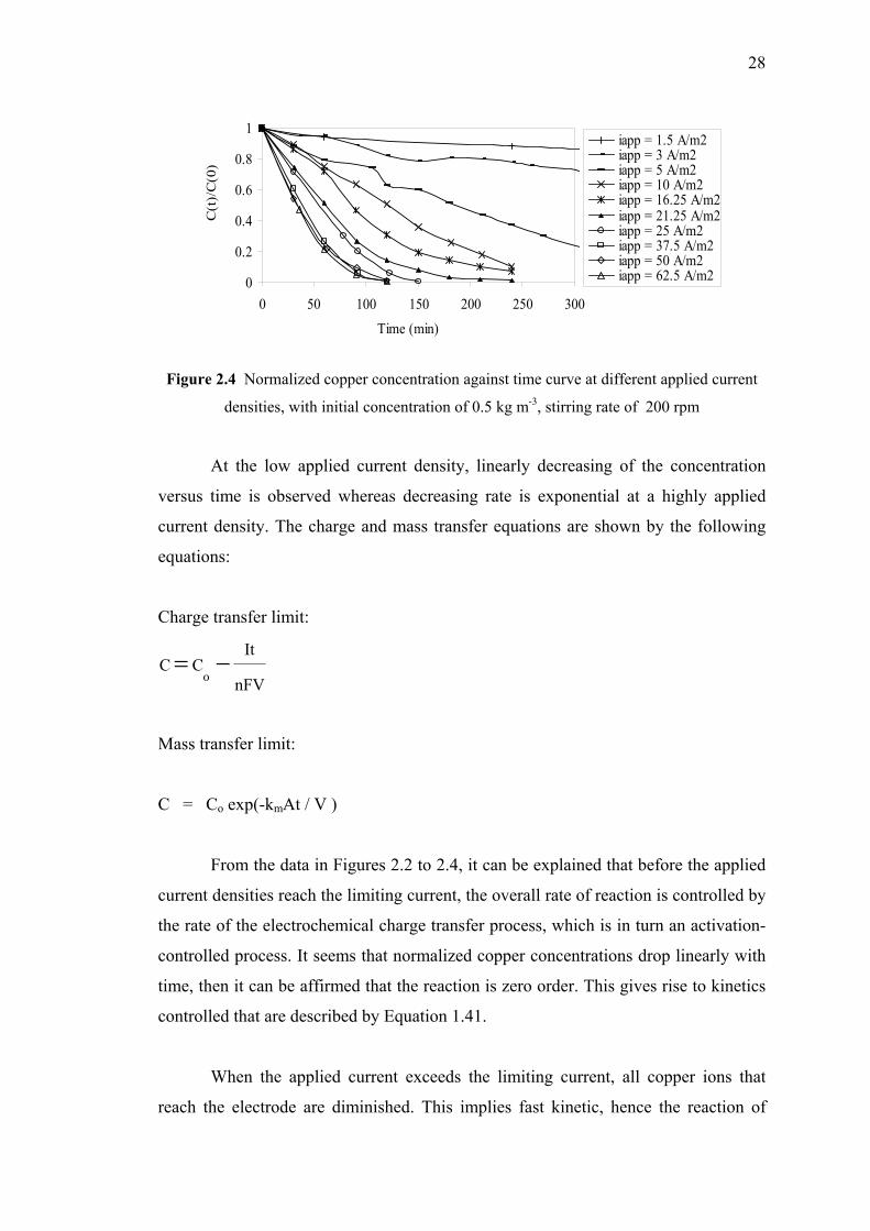
28

0

0.2

0.4

0.6

0.8

1

0 50 100 150 200 250 300

Time (min)

C(t

)/C

(0)

iapp = 1.5 A/m2iapp = 3 A/m2iapp = 5 A/m2iapp = 10 A/m2iapp = 16.25 A/m2iapp = 21.25 A/m2iapp = 25 A/m2iapp = 37.5 A/m2iapp = 50 A/m2iapp = 62.5 A/m2



At the low applied current density, linearly decreasing of the concentration

versus time is observed whereas decreasing rate is exponential at a highly applied

current density. The charge and mass transfer equations are shown by the following

equations:

Charge transfer limit:

nFVItCC

ο−=

Mass transfer limit:

C = Co exp(-kmAt / V )

From the data in Figures 2.2 to 2.4, it can be explained that before the applied

current densities reach the limiting current, the overall rate of reaction is controlled by

the rate of the electrochemical charge transfer process, which is in turn an activation-

controlled process. It seems that normalized copper concentrations drop linearly with

time, then it can be affirmed that the reaction is zero order. This gives rise to kinetics

controlled that are described by Equation 1.41.

When the applied current exceeds the limiting current, all copper ions that

reach the electrode are diminished. This implies fast kinetic, hence the reaction of

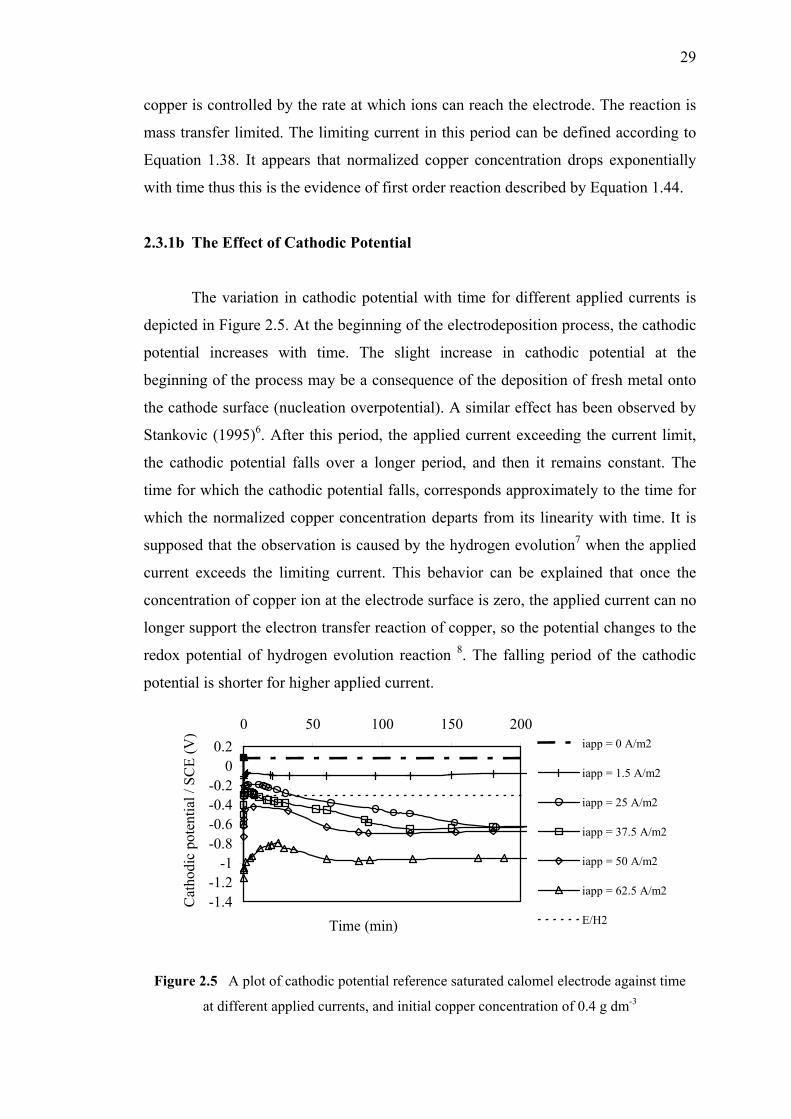
29

copper is controlled by the rate at which ions can reach the electrode. The reaction is

mass transfer limited. The limiting current in this period can be defined according to

Equation 1.38. It appears that normalized copper concentration drops exponentially

with time thus this is the evidence of first order reaction described by Equation 1.44.

2.3.1b The Effect of Cathodic Potential

The variation in cathodic potential with time for different applied currents is

depicted in Figure 2.5. At the beginning of the electrodeposition process, the cathodic

potential increases with time. The slight increase in cathodic potential at the

beginning of the process may be a consequence of the deposition of fresh metal onto

the cathode surface (nucleation overpotential). A similar effect has been observed by

Stankovic (1995)6. After this period, the applied current exceeding the current limit,

the cathodic potential falls over a longer period, and then it remains constant. The

time for which the cathodic potential falls, corresponds approximately to the time for

which the normalized copper concentration departs from its linearity with time. It is

supposed that the observation is caused by the hydrogen evolution7 when the applied

current exceeds the limiting current. This behavior can be explained that once the

concentration of copper ion at the electrode surface is zero, the applied current can no

longer support the electron transfer reaction of copper, so the potential changes to the

redox potential of hydrogen evolution reaction 8. The falling period of the cathodic

potential is shorter for higher applied current.

Figure 2.5 A plot of cathodic potential reference saturated calomel electrode against time

at different applied currents, and initial copper concentration of 0.4 g dm-3

-1.4-1.2

-1-0.8-0.6-0.4-0.2

00.2

0 50 100 150 200

Time (min)

Cat

hodi

c po

tent

ial /

SC

E (V

)

iapp = 0 A/m2

iapp = 1.5 A/m2

iapp = 25 A/m2

iapp = 37.5 A/m2

iapp = 50 A/m2

iapp = 62.5 A/m2

E/H2

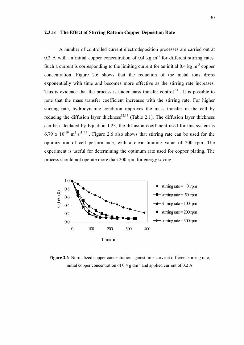
30

2.3.1c The Effect of Stirring Rate on Copper Deposition Rate

A number of controlled current electrodeposition processes are carried out at

0.2 A with an initial copper concentration of 0.4 kg m-3 for different stirring rates.

Such a current is corresponding to the limiting current for an initial 0.4 kg m-3 copper

concentration. Figure 2.6 shows that the reduction of the metal ions drops

exponentially with time and becomes more effective as the stirring rate increases.

This is evidence that the process is under mass transfer control9-11. It is possible to

note that the mass transfer coefficient increases with the stirring rate. For higher

stirring rate, hydrodynamic condition improves the mass transfer in the cell by

reducing the diffusion layer thickness12,13 (Table 2.1). The diffusion layer thickness

can be calculated by Equation 1.23, the diffusion coefficient used for this system is

6.79 x 10-10 m2 s-1 14 . Figure 2.6 also shows that stirring rate can be used for the

optimization of cell performance, with a clear limiting value of 200 rpm. The

experiment is useful for determining the optimum rate used for copper plating. The

process should not operate more than 200 rpm for energy saving.

Figure 2.6 Normalized copper concentration against time curve at different stirring rate,

initial copper concentration of 0.4 g dm-3 and applied current of 0.2 A

0.0

0.2

0.4

0.6

0.8

1.0

0 100 200 300 400

Time/min

C(t)

/C(0

)

stirring rate = 0 rpm





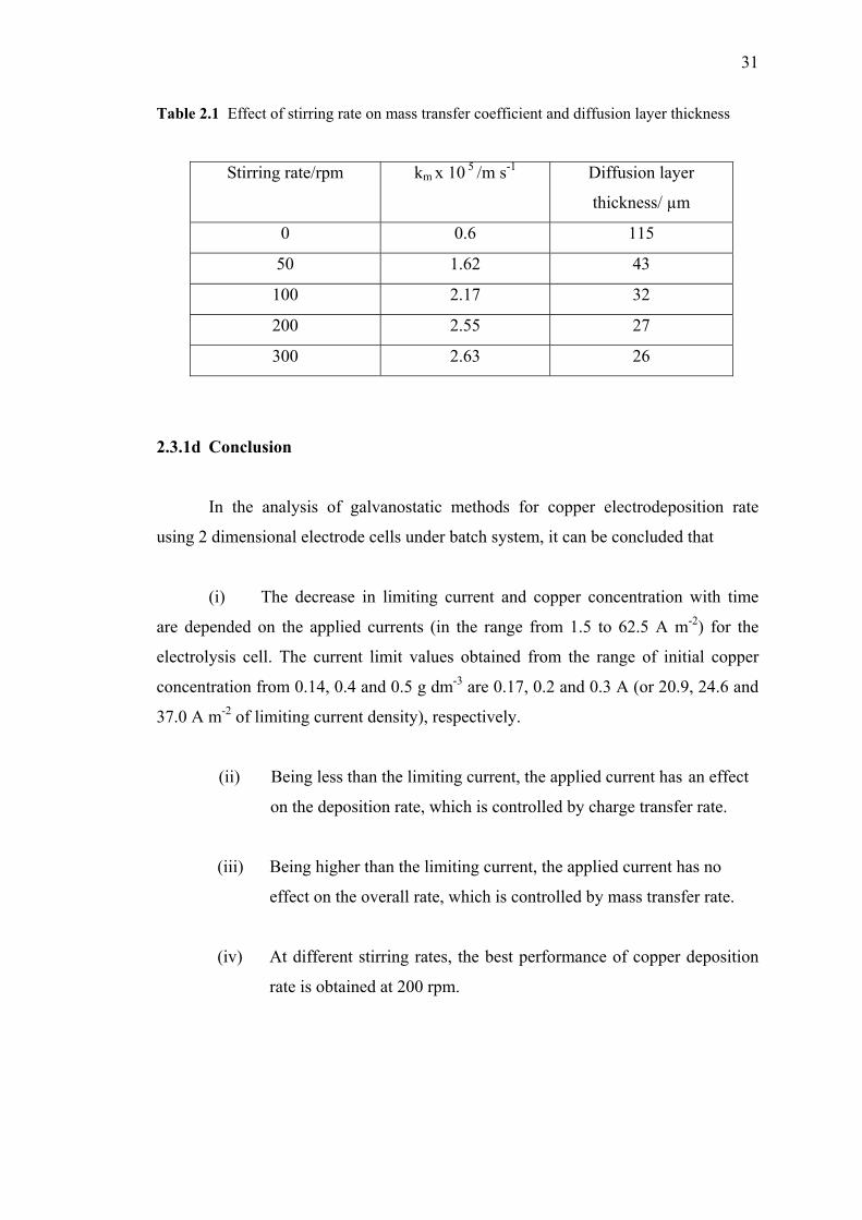
31

Table 2.1 Effect of stirring rate on mass transfer coefficient and diffusion layer thickness

Stirring rate/rpm km x 10 5 /m s-1 Diffusion layer

thickness/ µm

0 0.6 115

50 1.62 43

100 2.17 32

200 2.55 27

300 2.63 26

2.3.1d Conclusion

In the analysis of galvanostatic methods for copper electrodeposition rate

using 2 dimensional electrode cells under batch system, it can be concluded that

(i) The decrease in limiting current and copper concentration with time

are depended on the applied currents (in the range from 1.5 to 62.5 A m-2) for the

electrolysis cell. The current limit values obtained from the range of initial copper

concentration from 0.14, 0.4 and 0.5 g dm-3 are 0.17, 0.2 and 0.3 A (or 20.9, 24.6 and

37.0 A m-2 of limiting current density), respectively.

(ii) Being less than the limiting current, the applied current has an effect

on the deposition rate, which is controlled by charge transfer rate.

(iii) Being higher than the limiting current, the applied current has no

effect on the overall rate, which is controlled by mass transfer rate.

(iv) At different stirring rates, the best performance of copper deposition

rate is obtained at 200 rpm.

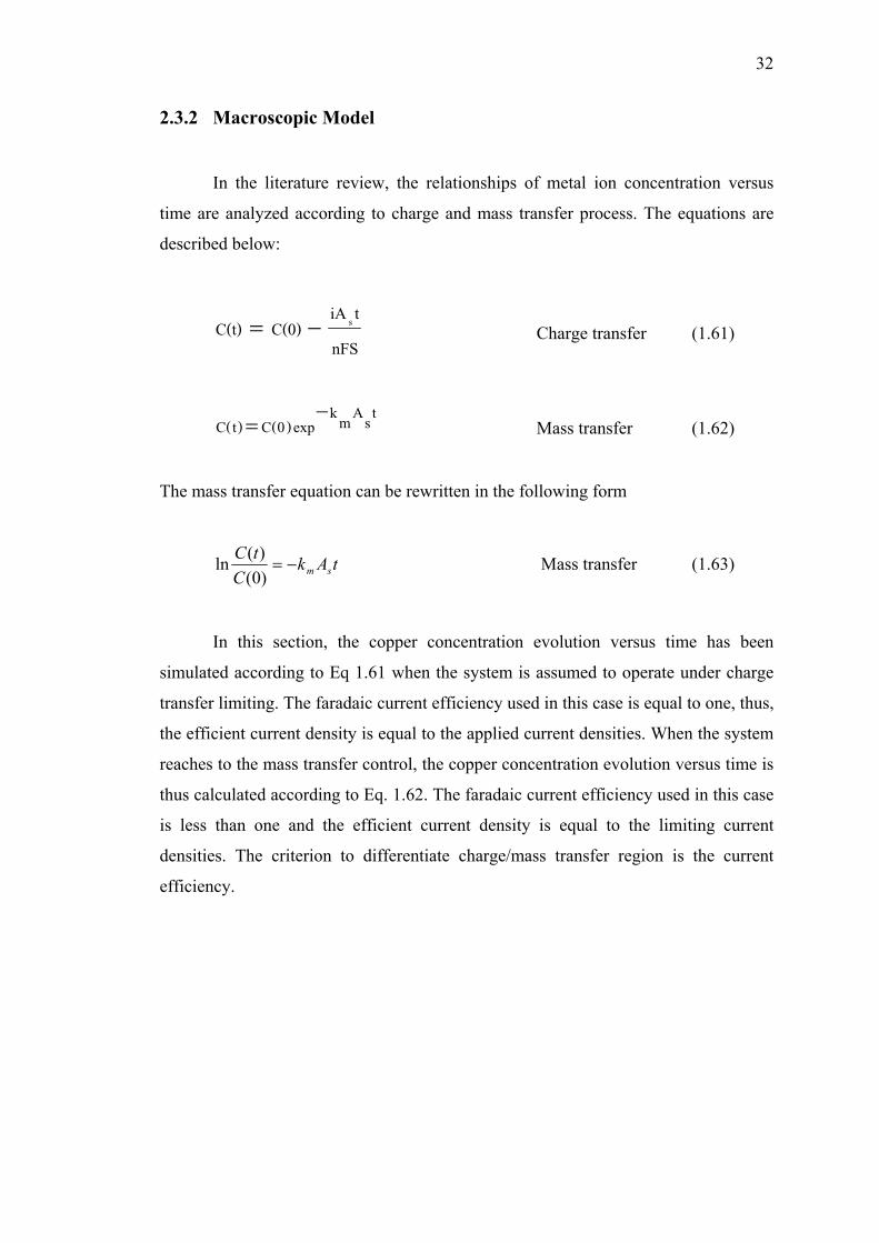
32

2.3.2 Macroscopic Model

In the literature review, the relationships of metal ion concentration versus

time are analyzed according to charge and mass transfer process. The equations are

described below:

nFStiAC(0)C(t) s−= Charge transfer (1.61)

tsAmkexp)(C)t(C −= 0 Mass transfer (1.62)

The mass transfer equation can be rewritten in the following form

tAkC

tCsm−=

)0()(ln Mass transfer (1.63)

In this section, the copper concentration evolution versus time has been

simulated according to Eq 1.61 when the system is assumed to operate under charge

transfer limiting. The faradaic current efficiency used in this case is equal to one, thus,

the efficient current density is equal to the applied current densities. When the system

reaches to the mass transfer control, the copper concentration evolution versus time is

thus calculated according to Eq. 1.62. The faradaic current efficiency used in this case

is less than one and the efficient current density is equal to the limiting current

densities. The criterion to differentiate charge/mass transfer region is the current

efficiency.

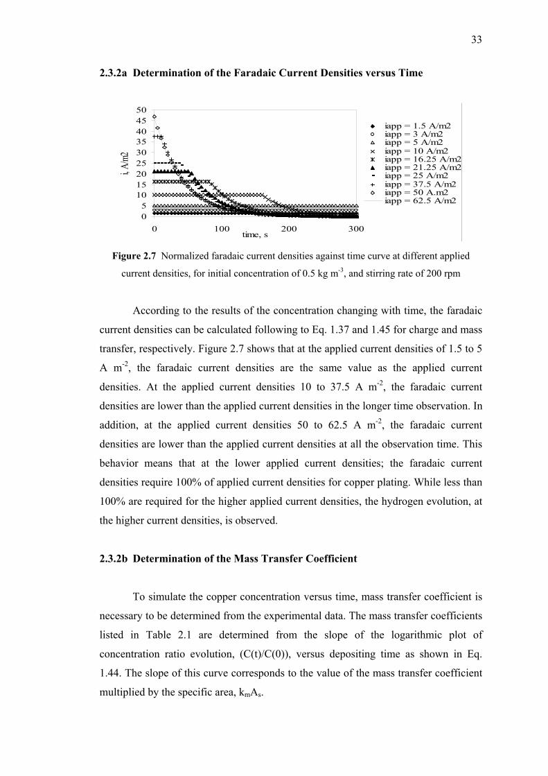
33

2.3.2a Determination of the Faradaic Current Densities versus Time

05

101520253035404550

0 100 200 300time, s

i, A/m

2iapp = 1.5 A/m2iapp = 3 A/m2iapp = 5 A/m2iapp = 10 A/m2iapp = 16.25 A/m2iapp = 21.25 A/m2iapp = 25 A/m2iapp = 37.5 A/m2iapp = 50 A.m2iapp = 62.5 A/m2

Figure 2.7 Normalized faradaic current densities against time curve at different applied

current densities, for initial concentration of 0.5 kg m-3, and stirring rate of 200 rpm

According to the results of the concentration changing with time, the faradaic

current densities can be calculated following to Eq. 1.37 and 1.45 for charge and mass

transfer, respectively. Figure 2.7 shows that at the applied current densities of 1.5 to 5

A m-2, the faradaic current densities are the same value as the applied current

densities. At the applied current densities 10 to 37.5 A m-2, the faradaic current

densities are lower than the applied current densities in the longer time observation. In

addition, at the applied current densities 50 to 62.5 A m-2, the faradaic current

densities are lower than the applied current densities at all the observation time. This

behavior means that at the lower applied current densities; the faradaic current

densities require 100% of applied current densities for copper plating. While less than

100% are required for the higher applied current densities, the hydrogen evolution, at

the higher current densities, is observed.

2.3.2b Determination of the Mass Transfer Coefficient

To simulate the copper concentration versus time, mass transfer coefficient is

necessary to be determined from the experimental data. The mass transfer coefficients

listed in Table 2.1 are determined from the slope of the logarithmic plot of

concentration ratio evolution, (C(t)/C(0)), versus depositing time as shown in Eq.

1.44. The slope of this curve corresponds to the value of the mass transfer coefficient

multiplied by the specific area, kmAs.

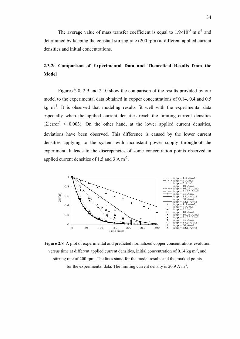
34

The average value of mass transfer coefficient is equal to 1.9×10-5 m s-1 and

determined by keeping the constant stirring rate (200 rpm) at different applied current

densities and initial concentrations.

2.3.2c Comparison of Experimental Data and Theoretical Results from the

Model

Figures 2.8, 2.9 and 2.10 show the comparison of the results provided by our

model to the experimental data obtained in copper concentrations of 0.14, 0.4 and 0.5

kg m-3. It is observed that modeling results fit well with the experimental data

especially when the applied current densities reach the limiting current densities

(∑ error2 < 0.003). On the other hand, at the lower applied current densities,

deviations have been observed. This difference is caused by the lower current

densities applying to the system with inconstant power supply throughout the

experiment. It leads to the discrepancies of some concentration points observed in

applied current densities of 1.5 and 3 A m-2.

0

0.2

0.4

0.6

0.8

1

0 50 100 150 200 250 300Time (min)

C(t)/

C(0)

iapp = 1.5 A/m2iapp = 3 A/m2iapp = 5 A/m2iapp = 10 A/m2iapp = 16.25 A/m2iapp = 21.25 A/m2iapp = 25 A/m2iapp = 37.5 A/m2iapp = 50 A/m2iapp = 62.5 A/m2iapp = 1.5 A/m2iapp = 3 A/m2iapp = 5A/m2iapp = 10 A/m2iapp = 16.25 A/m2iapp = 21.25 A/m2iapp = 25 A/m2iapp = 37.5 A/m2iapp = 50 A/m2iapp = 62.5 A/m2

Figure 2.8 A plot of experimental and predicted normalized copper concentrations evolution

versus time at different applied current densities, initial concentration of 0.14 kg m-3, and

stirring rate of 200 rpm. The lines stand for the model results and the marked points

for the experimental data. The limiting current density is 20.9 A m-2.

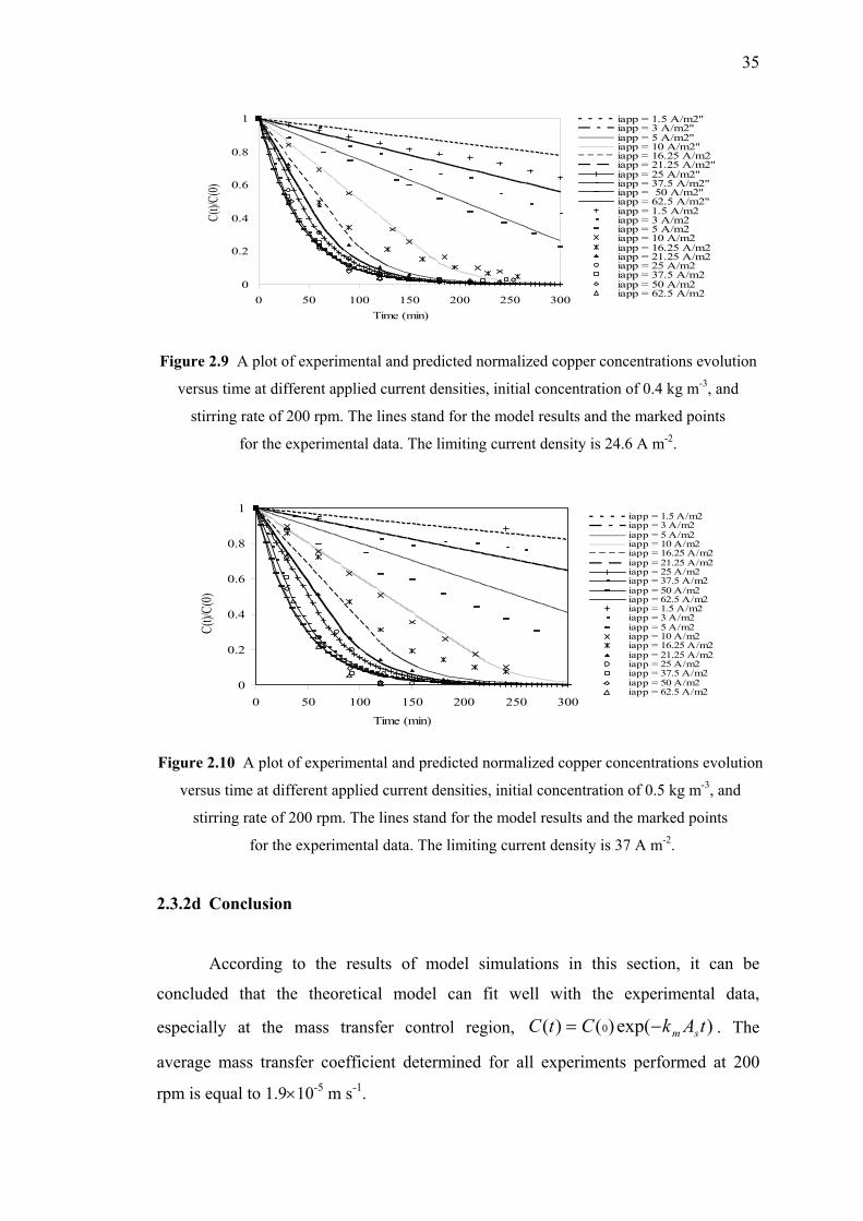
35

0

0.2

0.4

0.6

0.8

1

0 50 100 150 200 250 300Time (min)

C(t)/C

(0)

iapp = 1.5 A/m2"iapp = 3 A/m2"iapp = 5 A/m2"iapp = 10 A/m2"iapp = 16.25 A/m2iapp = 21.25 A/m2"iapp = 25 A/m2"iapp = 37.5 A/m2"iapp = 50 A/m2"iapp = 62.5 A/m2"iapp = 1.5 A/m2iapp = 3 A/m2iapp = 5 A/m2iapp = 10 A/m2iapp = 16.25 A/m2iapp = 21.25 A/m2iapp = 25 A/m2iapp = 37.5 A/m2iapp = 50 A/m2iapp = 62.5 A/m2




for the experimental data. The limiting current density is 24.6 A m-2.

0

0.2

0.4

0.6

0.8

1

0 50 100 150 200 250 300

Time (min)

C(t)/C

(0)

iapp = 1.5 A/m2iapp = 3 A/m2iapp = 5 A/m2iapp = 10 A/m2iapp = 16.25 A/m2iapp = 21.25 A/m2iapp = 25 A/m2iapp = 37.5 A/m2iapp = 50 A/m2iapp = 62.5 A/m2iapp = 1.5 A/m2iapp = 3 A/m2iapp = 5 A/m2iapp = 10 A/m2iapp = 16.25 A/m2iapp = 21.25 A/m2iapp = 25 A/m2iapp = 37.5 A/m2iapp = 50 A/m2iapp = 62.5 A/m2




for the experimental data. The limiting current density is 37 A m-2.

2.3.2d Conclusion

According to the results of model simulations in this section, it can be

concluded that the theoretical model can fit well with the experimental data,

especially at the mass transfer control region, )exp()()( 0 tAkCtC sm−= . The

average mass transfer coefficient determined for all experiments performed at 200

rpm is equal to 1.9×10-5 m s-1.

36

The application of this model is to monitor the decrease in concentration

versus time. As the concentration decreases, the properties of the bath are also

changed with time, diminishing the quality of the deposit. According to the model,

time duration, related to the lower concentration of reacting species in the bath, is

determined. This will guide towards an appropriate time of adding species into the

bath, to maintain their required concentration.

Conclusion

The general theory of the electrochemistry dealing with the charge transfer,

mass transfer and the electrochemical reactor, has been analyzed in the bibliography

part, chapter 1. The macroscopic model is used to investigate concentrations of metal

species at the bulk electrolyte versus time according to the role of charge and mass

transfer in the batch reactor.

In this part, the bulk concentration, in relation to efficient current, is monitored

versus time. The different characteristic of concentration evolution depends on the

type of electrochemical reactor. These characteristics can be applied for the

electrochemical process of metal recovery, and determined for time duration of

plating process and electrosynthesis.

The macroscopic model is not sufficient to explain the electrochemical

mechanism dealing with the reaction phenomenon on the electrode surface. In doing

so, the microscopic model is required and analyzed, as will be described in the part 3.

PART 2

ANALYSIS OF THE CURRENT DISTRIBUTION


Introduction

Electrochemical plating is used to give a particular surface property to a

component. This can be a decorative aspect (silver, gilding), a physical or mechanical

property different from an existing one (hard chromium), or a protection against

corrosion (nickel and chromium). The operating condition has an effect strongly on

the properties of the deposit. The current density is able to affect the morphology and

composition. It is often purposely carried out under non-uniform current distribution,

using electroplating test cells. In a single experiment, electroplaters can thus study the

effect of a wide range of current densities on deposit morphology and composition, to

save time13.

This section is composed of two main chapters. The first one concerns the

bibliography dealing with the different kinds of current distribution and Wagner

number, and the different kinds of electroplating reactors used in the electroplating

industry. The advantages and disadvantages of these electroplating reactors are also

discussed. The second chapter presents the experimental investigation consisting of

the current distribution in two particular reactors, the Mohler cell and the Rotating

Cylinder Hull cell.

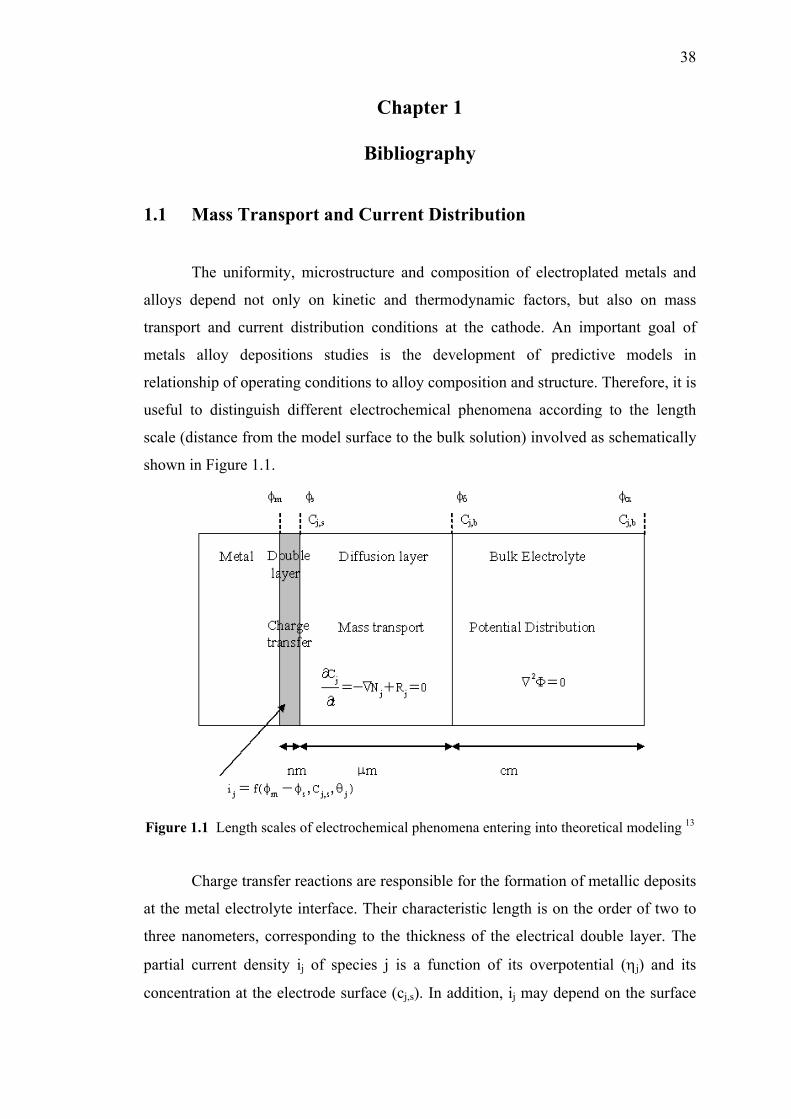
38

Chapter 1

Bibliography

1.1 Mass Transport and Current Distribution

The uniformity, microstructure and composition of electroplated metals and

alloys depend not only on kinetic and thermodynamic factors, but also on mass

transport and current distribution conditions at the cathode. An important goal of

metals alloy depositions studies is the development of predictive models in

relationship of operating conditions to alloy composition and structure. Therefore, it is

useful to distinguish different electrochemical phenomena according to the length

scale (distance from the model surface to the bulk solution) involved as schematically

shown in Figure 1.1.

Figure 1.1 Length scales of electrochemical phenomena entering into theoretical modeling 13

Charge transfer reactions are responsible for the formation of metallic deposits

at the metal electrolyte interface. Their characteristic length is on the order of two to

three nanometers, corresponding to the thickness of the electrical double layer. The

partial current density ij of species j is a function of its overpotential (ηj) and its

concentration at the electrode surface (cj,s). In addition, ij may depend on the surface

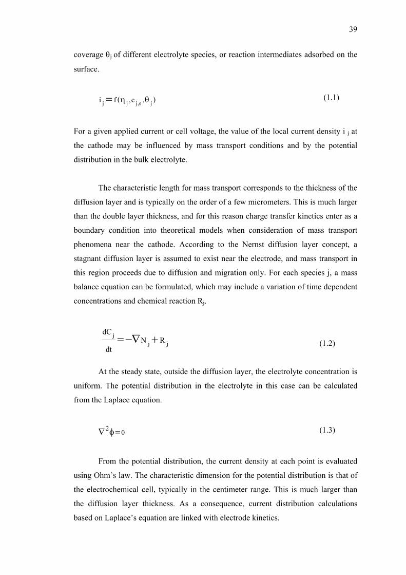
39

coverage θj of different electrolyte species, or reaction intermediates adsorbed on the

surface.

),c,(fi js,jjj θη= (1.1)

For a given applied current or cell voltage, the value of the local current density i j at

the cathode may be influenced by mass transport conditions and by the potential

distribution in the bulk electrolyte.

The characteristic length for mass transport corresponds to the thickness of the

diffusion layer and is typically on the order of a few micrometers. This is much larger

than the double layer thickness, and for this reason charge transfer kinetics enter as a

boundary condition into theoretical models when consideration of mass transport

phenomena near the cathode. According to the Nernst diffusion layer concept, a

stagnant diffusion layer is assumed to exist near the electrode, and mass transport in

this region proceeds due to diffusion and migration only. For each species j, a mass

balance equation can be formulated, which may include a variation of time dependent

concentrations and chemical reaction Rj.

(1.2)

At the steady state, outside the diffusion layer, the electrolyte concentration is

uniform. The potential distribution in the electrolyte in this case can be calculated

from the Laplace equation.

02 =φ∇ (1.3)

From the potential distribution, the current density at each point is evaluated

using Ohm’s law. The characteristic dimension for the potential distribution is that of

the electrochemical cell, typically in the centimeter range. This is much larger than

the diffusion layer thickness. As a consequence, current distribution calculations

based on Laplace’s equation are linked with electrode kinetics.

jjj RN

dtdC

+−∇=

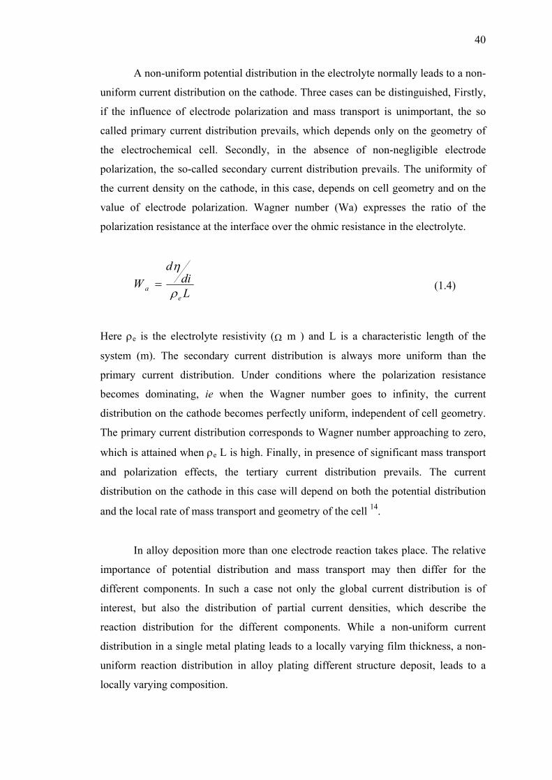
40

A non-uniform potential distribution in the electrolyte normally leads to a non-

uniform current distribution on the cathode. Three cases can be distinguished, Firstly,

if the influence of electrode polarization and mass transport is unimportant, the so

called primary current distribution prevails, which depends only on the geometry of

the electrochemical cell. Secondly, in the absence of non-negligible electrode

polarization, the so-called secondary current distribution prevails. The uniformity of

the current density on the cathode, in this case, depends on cell geometry and on the

value of electrode polarization. Wagner number (Wa) expresses the ratio of the

polarization resistance at the interface over the ohmic resistance in the electrolyte.

Ldi

dW

ea ρ

η= (1.4)

Here ρe is the electrolyte resistivity (Ω m ) and L is a characteristic length of the

system (m). The secondary current distribution is always more uniform than the

primary current distribution. Under conditions where the polarization resistance

becomes dominating, ie when the Wagner number goes to infinity, the current

distribution on the cathode becomes perfectly uniform, independent of cell geometry.

The primary current distribution corresponds to Wagner number approaching to zero,

which is attained when ρe L is high. Finally, in presence of significant mass transport

and polarization effects, the tertiary current distribution prevails. The current

distribution on the cathode in this case will depend on both the potential distribution

and the local rate of mass transport and geometry of the cell 14.

In alloy deposition more than one electrode reaction takes place. The relative

importance of potential distribution and mass transport may then differ for the

different components. In such a case not only the global current distribution is of

interest, but also the distribution of partial current densities, which describe the

reaction distribution for the different components. While a non-uniform current

distribution in a single metal plating leads to a locally varying film thickness, a non-

uniform reaction distribution in alloy plating different structure deposit, leads to a

locally varying composition.

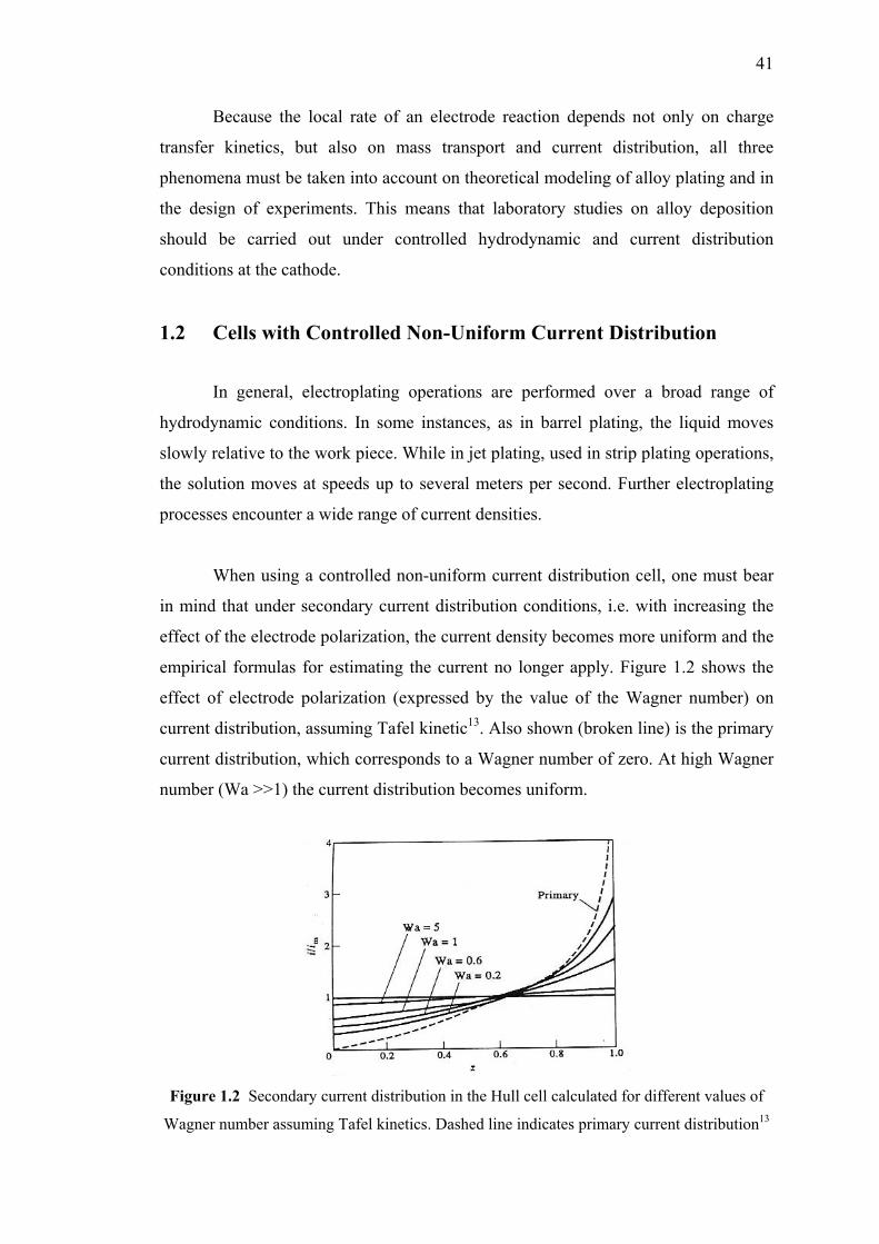
41

Because the local rate of an electrode reaction depends not only on charge

transfer kinetics, but also on mass transport and current distribution, all three

phenomena must be taken into account on theoretical modeling of alloy plating and in

the design of experiments. This means that laboratory studies on alloy deposition

should be carried out under controlled hydrodynamic and current distribution

conditions at the cathode.

1.2 Cells with Controlled Non-Uniform Current Distribution

In general, electroplating operations are performed over a broad range of

hydrodynamic conditions. In some instances, as in barrel plating, the liquid moves

slowly relative to the work piece. While in jet plating, used in strip plating operations,

the solution moves at speeds up to several meters per second. Further electroplating

processes encounter a wide range of current densities.

When using a controlled non-uniform current distribution cell, one must bear

in mind that under secondary current distribution conditions, i.e. with increasing the

effect of the electrode polarization, the current density becomes more uniform and the

empirical formulas for estimating the current no longer apply. Figure 1.2 shows the

effect of electrode polarization (expressed by the value of the Wagner number) on

current distribution, assuming Tafel kinetic13. Also shown (broken line) is the primary

current distribution, which corresponds to a Wagner number of zero. At high Wagner

number (Wa >>1) the current distribution becomes uniform.

Figure 1.2 Secondary current distribution in the Hull cell calculated for different values of

Wagner number assuming Tafel kinetics. Dashed line indicates primary current distribution13

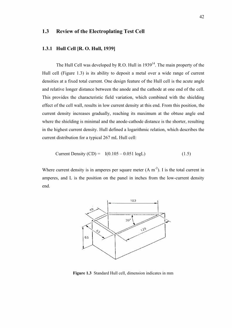
42

1.3 Review of the Electroplating Test Cell

1.3.1 Hull Cell [R. O. Hull, 1939]

The Hull Cell was developed by R.O. Hull in 193914. The main property of the

Hull cell (Figure 1.3) is its ability to deposit a metal over a wide range of current

densities at a fixed total current. One design feature of the Hull cell is the acute angle

and relative longer distance between the anode and the cathode at one end of the cell.

This provides the characteristic field variation, which combined with the shielding

effect of the cell wall, results in low current density at this end. From this position, the

current density increases gradually, reaching its maximum at the obtuse angle end

where the shielding is minimal and the anode-cathode distance is the shorter, resulting

in the highest current density. Hull defined a logarithmic relation, which describes the

current distribution for a typical 267 mL Hull cell:

Current Density (CD) = I(0.105 – 0.051 logL) (1.5)

Where current density is in amperes per square meter (A m-2). I is the total current in

amperes, and L is the position on the panel in inches from the low-current density

end.

Figure 1.3 Standard Hull cell, dimension indicates in mm

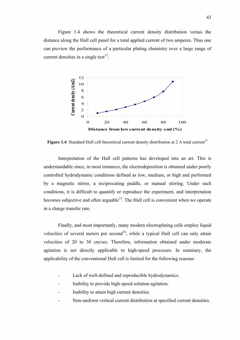
43

Figure 1.4 shows the theoretical current density distribution versus the

distance along the Hull cell panel for a total applied current of two amperes. Thus one

can preview the performance of a particular plating chemistry over a large range of

current densities in a single test13.

0

2

4

6

8

10

12

0 20 40 60 80 100

Distance from low current density end (%)

Curre

nt de

nsity

(A/m

2)

Figure 1.4 Standard Hull cell theoretical current density distribution at 2 A total current15

Interpretation of the Hull cell patterns has developed into an art. This is

understandable since, in most instances, the electrodeposition is obtained under poorly

controlled hydrodynamic conditions defined as low, medium, or high and performed

by a magnetic stirrer, a reciprocating paddle, or manual stirring. Under such

conditions, it is difficult to quantify or reproduce the experiment, and interpretation

becomes subjective and often arguable15. The Hull cell is convenient when we operate

in a charge transfer rate.

Finally, and most importantly, many modern electroplating cells employ liquid

velocities of several meters per second16, while a typical Hull cell can only attain

velocities of 20 to 30 cm/sec. Therefore, information obtained under moderate

agitation is not directly applicable to high-speed processes. In summary, the

applicability of the conventional Hull cell is limited for the following reasons:

- Lack of well-defined and reproducible hydrodynamics.

- Inability to provide high-speed solution agitation.

- Inability to attain high current densities.

- Non-uniform vertical current distribution at specified current densities.

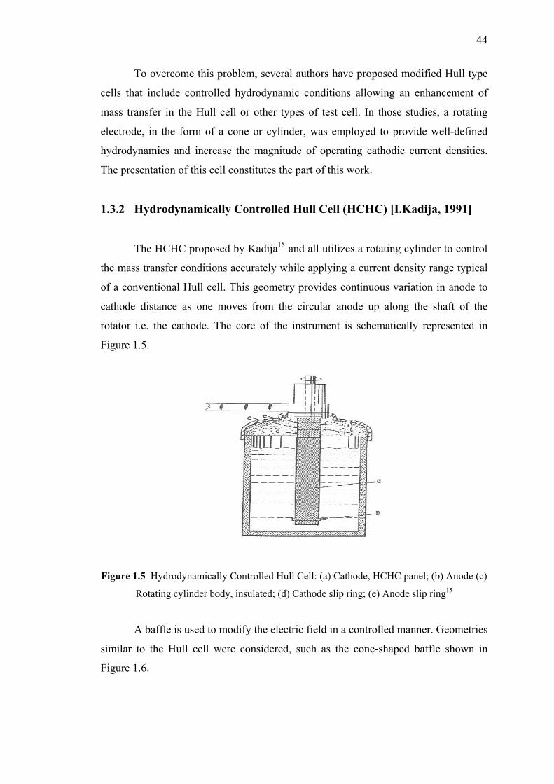
44

To overcome this problem, several authors have proposed modified Hull type

cells that include controlled hydrodynamic conditions allowing an enhancement of

mass transfer in the Hull cell or other types of test cell. In those studies, a rotating

electrode, in the form of a cone or cylinder, was employed to provide well-defined

hydrodynamics and increase the magnitude of operating cathodic current densities.

The presentation of this cell constitutes the part of this work.

1.3.2 Hydrodynamically Controlled Hull Cell (HCHC) [I.Kadija, 1991]

The HCHC proposed by Kadija15 and all utilizes a rotating cylinder to control

the mass transfer conditions accurately while applying a current density range typical

of a conventional Hull cell. This geometry provides continuous variation in anode to

cathode distance as one moves from the circular anode up along the shaft of the

rotator i.e. the cathode. The core of the instrument is schematically represented in

Figure 1.5.

Figure 1.5 Hydrodynamically Controlled Hull Cell: (a) Cathode, HCHC panel; (b) Anode (c)

Rotating cylinder body, insulated; (d) Cathode slip ring; (e) Anode slip ring15

A baffle is used to modify the electric field in a controlled manner. Geometries

similar to the Hull cell were considered, such as the cone-shaped baffle shown in

Figure 1.6.

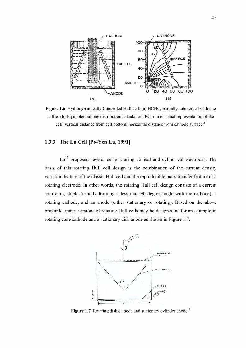
45

Figure 1.6 Hydrodynamically Controlled Hull cell: (a) HCHC, partially submerged with one

baffle; (b) Equipotential line distribution calculation; two-dimensional representation of the

cell: vertical distance from cell bottom; horizontal distance from cathode surface15

1.3.3 The Lu Cell [Po-Yen Lu, 1991]

Lu17 proposed several designs using conical and cylindrical electrodes. The

basis of this rotating Hull cell design is the combination of the current density

variation feature of the classic Hull cell and the reproducible mass transfer feature of a

rotating electrode. In other words, the rotating Hull cell design consists of a current

restricting shield (usually forming a less than 90 degree angle with the cathode), a

rotating cathode, and an anode (either stationary or rotating). Based on the above

principle, many versions of rotating Hull cells may be designed as for an example in

rotating cone cathode and a stationary disk anode as shown in Figure 1.7.

Figure 1.7 Rotating disk cathode and stationary cylinder anode17

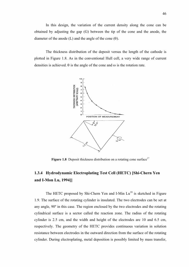
46

In this design, the variation of the current density along the cone can be

obtained by adjusting the gap (G) between the tip of the cone and the anode, the

diameter of the anode (L) and the angle of the cone (θ).

The thickness distribution of the deposit versus the length of the cathode is

plotted in Figure 1.8. As in the conventional Hull cell, a very wide range of current

densities is achieved. θ is the angle of the cone and ω is the rotation rate.

Figure 1.8 Deposit thickness distribution on a rotating cone surface17

1.3.4 Hydrodynamic Electroplating Test Cell (HETC) [Shi-Chern Yen

and I-Mon Lu, 1994]]

The HETC proposed by Shi-Chern Yen and I-Min Lu18 is sketched in Figure

1.9. The surface of the rotating cylinder is insulated. The two electrodes can be set at

any angle, 90º in this case. The region enclosed by the two electrodes and the rotating

cylindrical surface is a sector called the reaction zone. The radius of the rotating

cylinder is 2.5 cm, and the width and height of the electrodes are 10 and 6.5 cm,

respectively. The geometry of the HETC provides continuous variation in solution

resistance between electrodes in the outward direction from the surface of the rotating

cylinder. During electroplating, metal deposition is possibly limited by mass transfer,

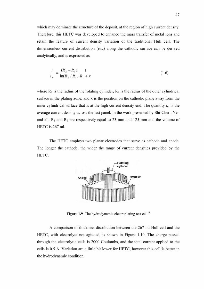
47

which may dominate the structure of the deposit, at the region of high current density.

Therefore, this HETC was developed to enhance the mass transfer of metal ions and

retain the feature of current density variation of the traditional Hull cell. The

dimensionless current distribution (i/im) along the cathodic surface can be derived

analytically, and is expressed as

xRRR

RRiim +

−=

112

12 1)/ln(

)( (1.6)

where R1 is the radius of the rotating cylinder, R2 is the radius of the outer cylindrical

surface in the plating zone, and x is the position on the cathodic plane away from the

inner cylindrical surface that is at the high current density end. The quantity im is the

average current density across the test panel. In the work presented by Shi-Chern Yen

and all, R1 and R2 are respectively equal to 23 mm and 125 mm and the volume of

HETC is 267 ml.

The HETC employs two planar electrodes that serve as cathode and anode.

The longer the cathode, the wider the range of current densities provided by the

HETC.

Figure 1.9 The hydrodynamic electroplating test cell18

A comparison of thickness distribution between the 267 ml Hull cell and the

HETC, with electrolyte not agitated, is shown in Figure 1.10. The charge passed

through the electrolytic cells is 2000 Coulombs, and the total current applied to the

cells is 0.5 A. Variation are a little bit lower for HETC, however this cell is better in

the hydrodynamic condition.

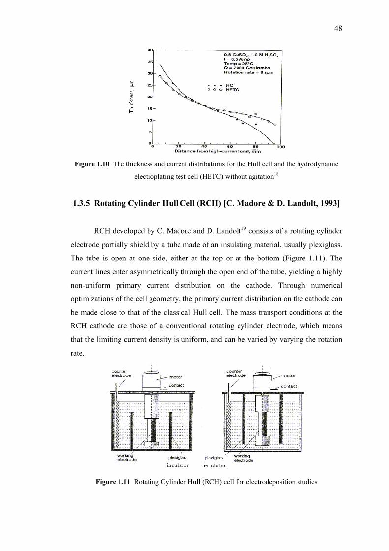
48

Figure 1.10 The thickness and current distributions for the Hull cell and the hydrodynamic

electroplating test cell (HETC) without agitation18

1.3.5 Rotating Cylinder Hull Cell (RCH) [C. Madore & D. Landolt, 1993]

RCH developed by C. Madore and D. Landolt19 consists of a rotating cylinder

electrode partially shield by a tube made of an insulating material, usually plexiglass.

The tube is open at one side, either at the top or at the bottom (Figure 1.11). The

current lines enter asymmetrically through the open end of the tube, yielding a highly

non-uniform primary current distribution on the cathode. Through numerical

optimizations of the cell geometry, the primary current distribution on the cathode can

be made close to that of the classical Hull cell. The mass transport conditions at the

RCH cathode are those of a conventional rotating cylinder electrode, which means

that the limiting current density is uniform, and can be varied by varying the rotation

rate.

Figure 1.11 Rotating Cylinder Hull (RCH) cell for electrodeposition studies

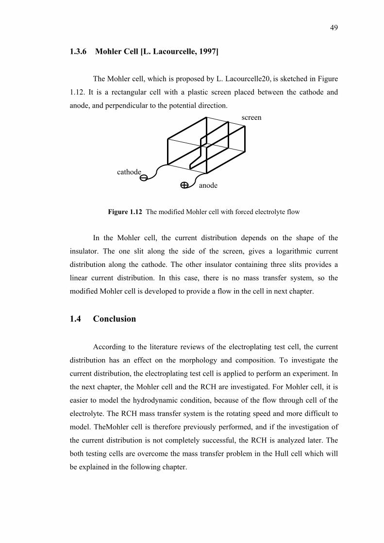
49

1.3.6 Mohler Cell [L. Lacourcelle, 1997]

The Mohler cell, which is proposed by L. Lacourcelle20, is sketched in Figure

1.12. It is a rectangular cell with a plastic screen placed between the cathode and

anode, and perpendicular to the potential direction.

Figure 1.12 The modified Mohler cell with forced electrolyte flow

In the Mohler cell, the current distribution depends on the shape of the

insulator. The one slit along the side of the screen, gives a logarithmic current

distribution along the cathode. The other insulator containing three slits provides a

linear current distribution. In this case, there is no mass transfer system, so the

modified Mohler cell is developed to provide a flow in the cell in next chapter.

1.4 Conclusion

According to the literature reviews of the electroplating test cell, the current

distribution has an effect on the morphology and composition. To investigate the

current distribution, the electroplating test cell is applied to perform an experiment. In

the next chapter, the Mohler cell and the RCH are investigated. For Mohler cell, it is

easier to model the hydrodynamic condition, because of the flow through cell of the

electrolyte. The RCH mass transfer system is the rotating speed and more difficult to

model. TheMohler cell is therefore previously performed, and if the investigation of

the current distribution is not completely successful, the RCH is analyzed later. The

both testing cells are overcome the mass transfer problem in the Hull cell which will

be explained in the following chapter.

cathode

anode

screen

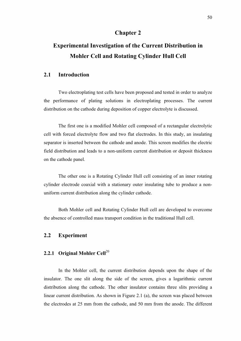
50

Chapter 2

Experimental Investigation of the Current Distribution in

Mohler Cell and Rotating Cylinder Hull Cell

2.1 Introduction

Two electroplating test cells have been proposed and tested in order to analyze

the performance of plating solutions in electroplating processes. The current

distribution on the cathode during deposition of copper electrolyte is discussed.

The first one is a modified Mohler cell composed of a rectangular electrolytic

cell with forced electrolyte flow and two flat electrodes. In this study, an insulating

separator is inserted between the cathode and anode. This screen modifies the electric

field distribution and leads to a non-uniform current distribution or deposit thickness

on the cathode panel.

The other one is a Rotating Cylinder Hull cell consisting of an inner rotating

cylinder electrode coaxial with a stationary outer insulating tube to produce a non-

uniform current distribution along the cylinder cathode.

Both Mohler cell and Rotating Cylinder Hull cell are developed to overcome

the absence of controlled mass transport condition in the traditional Hull cell.

2.2 Experiment

2.2.1 Original Mohler Cell20

In the Mohler cell, the current distribution depends upon the shape of the

insulator. The one slit along the side of the screen, gives a logarithmic current

distribution along the cathode. The other insulator contains three slits providing a

linear current distribution. As shown in Figure 2.1 (a), the screen was placed between

the electrodes at 25 mm from the cathode, and 50 mm from the anode. The different

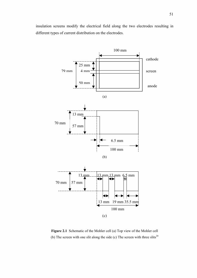
51

insulation screens modify the electrical field along the two electrodes resulting in

different types of current distribution on the electrodes.

(a)

(b)

(c)

Figure 2.1 Schematic of the Mohler cell (a) Top view of the Mohler cell

(b) The screen with one slit along the side (c) The screen with three slits20

100 mm

70 mm 57 mm

13 mm 13 mm 13 mm 6.5 mm

13 mm 19 mm 35.5 mm

100 mm

6.5 mm

70 mm 57 mm

13 mm

79 mm 4 mm 25 mm

100 mm

cathode

screen

anode 50 mm

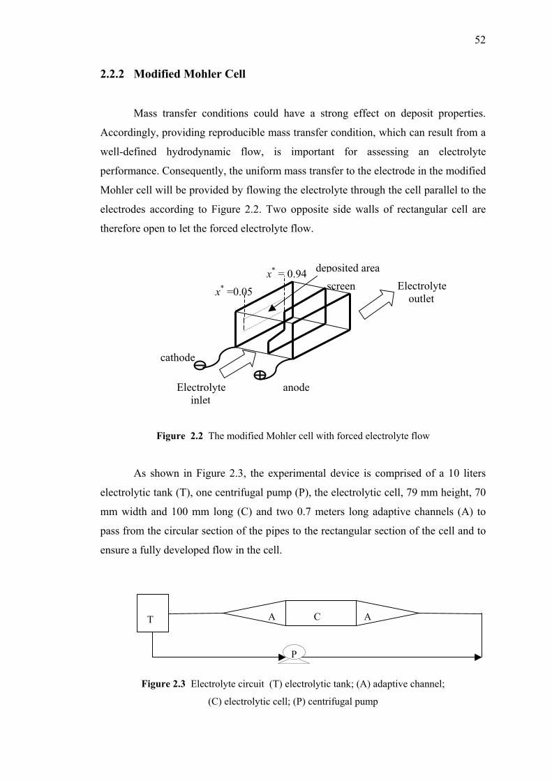
52

2.2.2 Modified Mohler Cell

Mass transfer conditions could have a strong effect on deposit properties.

Accordingly, providing reproducible mass transfer condition, which can result from a

well-defined hydrodynamic flow, is important for assessing an electrolyte

performance. Consequently, the uniform mass transfer to the electrode in the modified

Mohler cell will be provided by flowing the electrolyte through the cell parallel to the

electrodes according to Figure 2.2. Two opposite side walls of rectangular cell are

therefore open to let the forced electrolyte flow.

Figure 2.2 The modified Mohler cell with forced electrolyte flow

As shown in Figure 2.3, the experimental device is comprised of a 10 liters

electrolytic tank (T), one centrifugal pump (P), the electrolytic cell, 79 mm height, 70

mm width and 100 mm long (C) and two 0.7 meters long adaptive channels (A) to

pass from the circular section of the pipes to the rectangular section of the cell and to

ensure a fully developed flow in the cell.

Figure 2.3 Electrolyte circuit (T) electrolytic tank; (A) adaptive channel;

(C) electrolytic cell; (P) centrifugal pump

Electrolyte inlet

cathode

anode

screen Electrolyte outlet

deposited area

x* =0.05x* = 0.94

T A C A

P

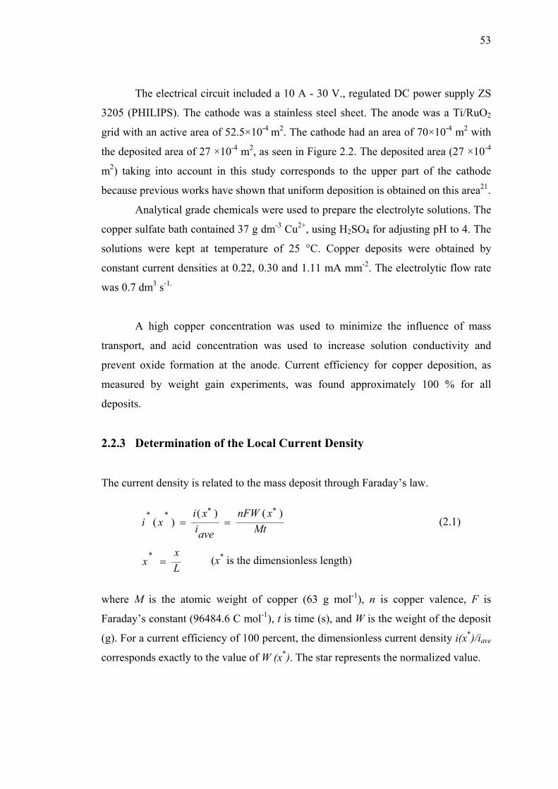
53

The electrical circuit included a 10 A - 30 V., regulated DC power supply ZS

3205 (PHILIPS). The cathode was a stainless steel sheet. The anode was a Ti/RuO2

grid with an active area of 52.5×10-4 m2. The cathode had an area of 70×10-4 m2 with

the deposited area of 27 ×10-4 m2, as seen in Figure 2.2. The deposited area (27 ×10-4

m2) taking into account in this study corresponds to the upper part of the cathode

because previous works have shown that uniform deposition is obtained on this area21.

Analytical grade chemicals were used to prepare the electrolyte solutions. The

copper sulfate bath contained 37 g dm-3 Cu2+, using H2SO4 for adjusting pH to 4. The

solutions were kept at temperature of 25 °C. Copper deposits were obtained by

constant current densities at 0.22, 0.30 and 1.11 mA mm-2. The electrolytic flow rate

was 0.7 dm3 s-1.

A high copper concentration was used to minimize the influence of mass

transport, and acid concentration was used to increase solution conductivity and

prevent oxide formation at the anode. Current efficiency for copper deposition, as

measured by weight gain experiments, was found approximately 100 % for all

deposits.

2.2.3 Determination of the Local Current Density

The current density is related to the mass deposit through Faraday’s law.

(2.1)

(x* is the dimensionless length)

where M is the atomic weight of copper (63 g mol-1), n is copper valence, F is

Faraday’s constant (96484.6 C mol-1), t is time (s), and W is the weight of the deposit

(g). For a current efficiency of 100 percent, the dimensionless current density i(x*)/iave

corresponds exactly to the value of W (x*). The star represents the normalized value.

Lx

x

MtxnFW

aveixi

xi

=

==

∗

∗∗ )()()(

**

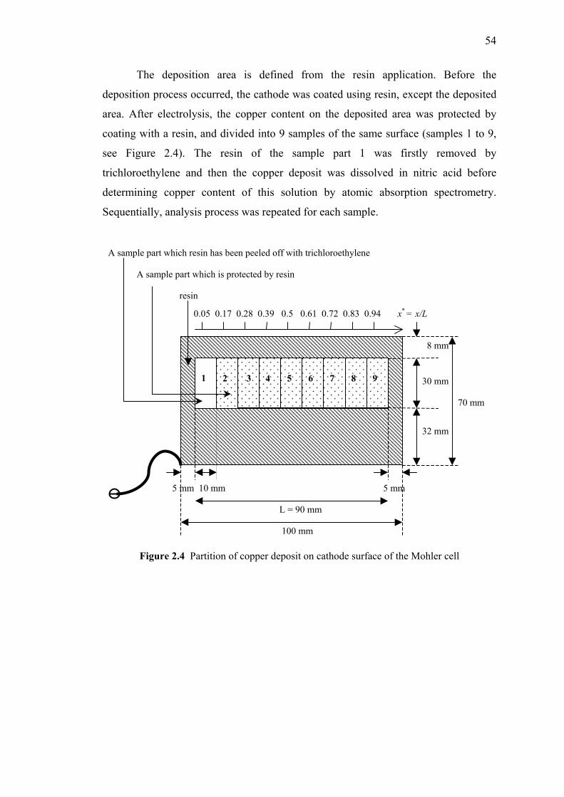
54

The deposition area is defined from the resin application. Before the

deposition process occurred, the cathode was coated using resin, except the deposited

area. After electrolysis, the copper content on the deposited area was protected by

coating with a resin, and divided into 9 samples of the same surface (samples 1 to 9,

see Figure 2.4). The resin of the sample part 1 was firstly removed by

trichloroethylene and then the copper deposit was dissolved in nitric acid before

determining copper content of this solution by atomic absorption spectrometry.

Sequentially, analysis process was repeated for each sample.

Figure 2.4 Partition of copper deposit on cathode surface of the Mohler cell

2

1

5 mm 10 mm 5 mm

100 mm

8 mm

A sample part which is protected by resin

A sample part which resin has been peeled off with trichloroethylene

3

4

5

6

7

8

9

resin

32 mm

30 mm

L = 90 mm

0.05 0.17 0.28 0.39 0.5 0.61 0.72 0.83 0.94 x* = x/L

70 mm

55


2.3.1 Current Distributions in the Mohler Cell

In order to verify the linear current distribution in the Mohler cell, the three

slits screen was used. Figure 2.5 shows the experimental dimensionless current

density (i(x*)/iave) versus the dimensionless length (x* = x/L) along the cathode for

different total applied currents, iave correspond to the average current density

corresponding to the ratio of the total current intensity over the deposited area. From

this figure, it is apparent that the metal distribution along the length of the cathode

decreases from the inlet to the half of the cell, and an increase in the observed current

occurs beyond this point.

0.500

1.000

1.500

0 0.2 0.4 0.6 0.8 1x*

i(x*)

/iave

iave = 0.22 mA mm-2 iave = 0.30 mA mm-2 iave = 1.11 mA mm-2

Figure 2.5 Dependence of dimensionless current density distribution versus dimensionless

distance for various average current densities

The variation of current density versus the reduced distance does not produce

a linear current distribution. The local current density is found to vary within a range

from about 0.18 to 1.33 mA mm -2 for average deposition current densities ranging

from 0.22 to 1.11 mA mm -2. It is found that the ratio of the maximum (obtained at x*

= 0.05) to the minimum dimensionless current density (corresponding to x* = 0.5) is

only 2. Thus, the current variation at the cathode does not have a wide range for each

average current studied. In addition, there is border effect at the inlet and outlet of the

cathode, that is clearly seen by the increasing of current at x* = 0.05 and 0.94

respectively.

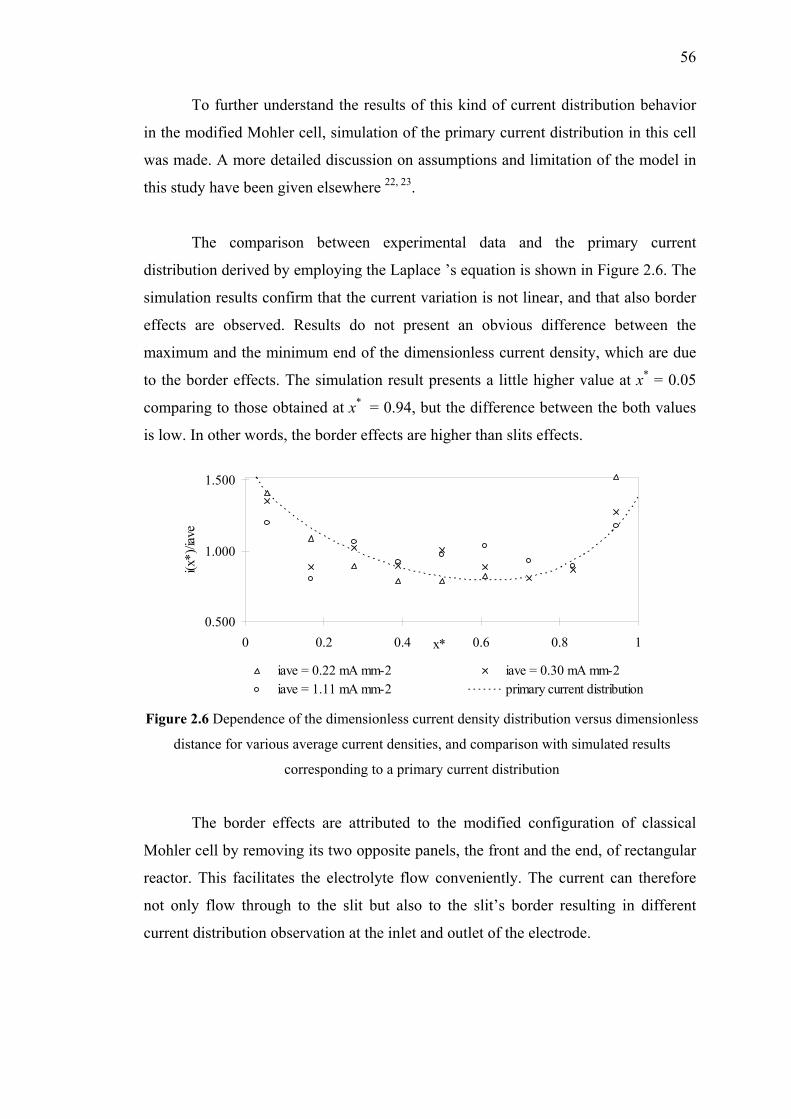
56

To further understand the results of this kind of current distribution behavior

in the modified Mohler cell, simulation of the primary current distribution in this cell

was made. A more detailed discussion on assumptions and limitation of the model in

this study have been given elsewhere 22, 23.

The comparison between experimental data and the primary current

distribution derived by employing the Laplace ’s equation is shown in Figure 2.6. The

simulation results confirm that the current variation is not linear, and that also border

effects are observed. Results do not present an obvious difference between the

maximum and the minimum end of the dimensionless current density, which are due

to the border effects. The simulation result presents a little higher value at x* = 0.05

comparing to those obtained at x* = 0.94, but the difference between the both values

is low. In other words, the border effects are higher than slits effects.

0.500

1.000

1.500

0 0.2 0.4 0.6 0.8 1x*

i(x*)

/iave

iave = 0.22 mA mm-2 iave = 0.30 mA mm-2iave = 1.11 mA mm-2 primary current distribution

Figure 2.6 Dependence of the dimensionless current density distribution versus dimensionless

distance for various average current densities, and comparison with simulated results

corresponding to a primary current distribution

The border effects are attributed to the modified configuration of classical

Mohler cell by removing its two opposite panels, the front and the end, of rectangular

reactor. This facilitates the electrolyte flow conveniently. The current can therefore

not only flow through to the slit but also to the slit’s border resulting in different

current distribution observation at the inlet and outlet of the electrode.

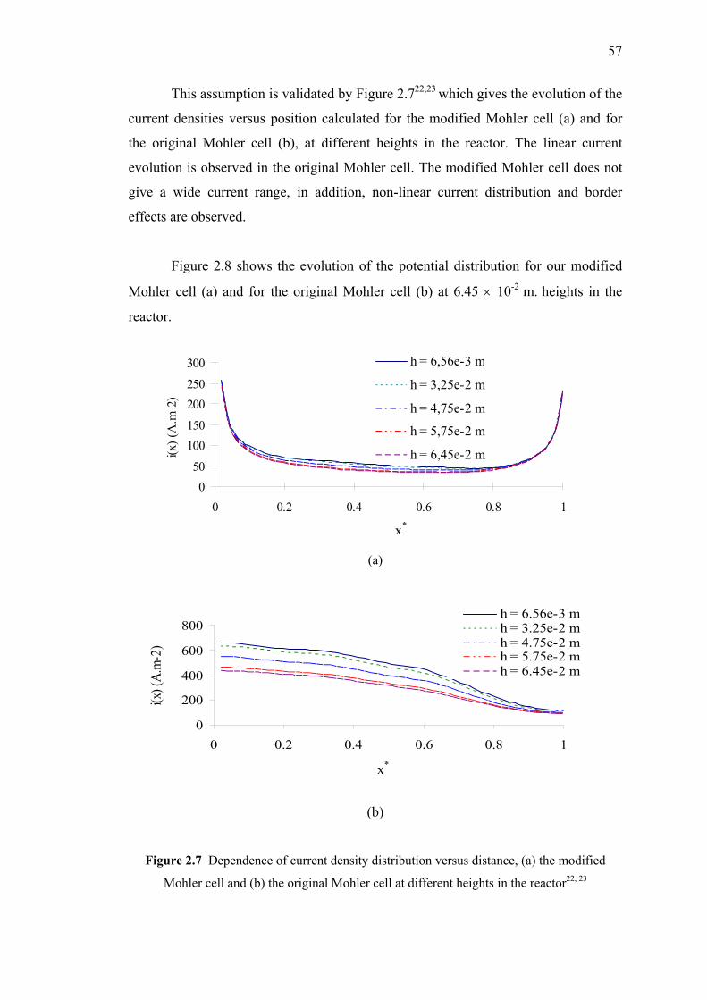
57

This assumption is validated by Figure 2.722,23 which gives the evolution of the

current densities versus position calculated for the modified Mohler cell (a) and for

the original Mohler cell (b), at different heights in the reactor. The linear current

evolution is observed in the original Mohler cell. The modified Mohler cell does not

give a wide current range, in addition, non-linear current distribution and border

effects are observed.

Figure 2.8 shows the evolution of the potential distribution for our modified

Mohler cell (a) and for the original Mohler cell (b) at 6.45 × 10-2 m. heights in the

reactor.

050

100150

200250

300

0 0.2 0.4 0.6 0.8 1

x (m)

i(x) (

A.m

-2)

h = 6,56e-3 m

h = 3,25e-2 m

h = 4,75e-2 m

h = 5,75e-2 m

h = 6,45e-2 m

(a)

0

200

400

600

800

0 0.2 0.4 0.6 0.8 1

x (m)

i(x) (

A.m-

2)

h = 6.56e-3 mh = 3.25e-2 mh = 4.75e-2 mh = 5.75e-2 mh = 6.45e-2 m

(b)

Figure 2.7 Dependence of current density distribution versus distance, (a) the modified

Mohler cell and (b) the original Mohler cell at different heights in the reactor22, 23

x*

x*

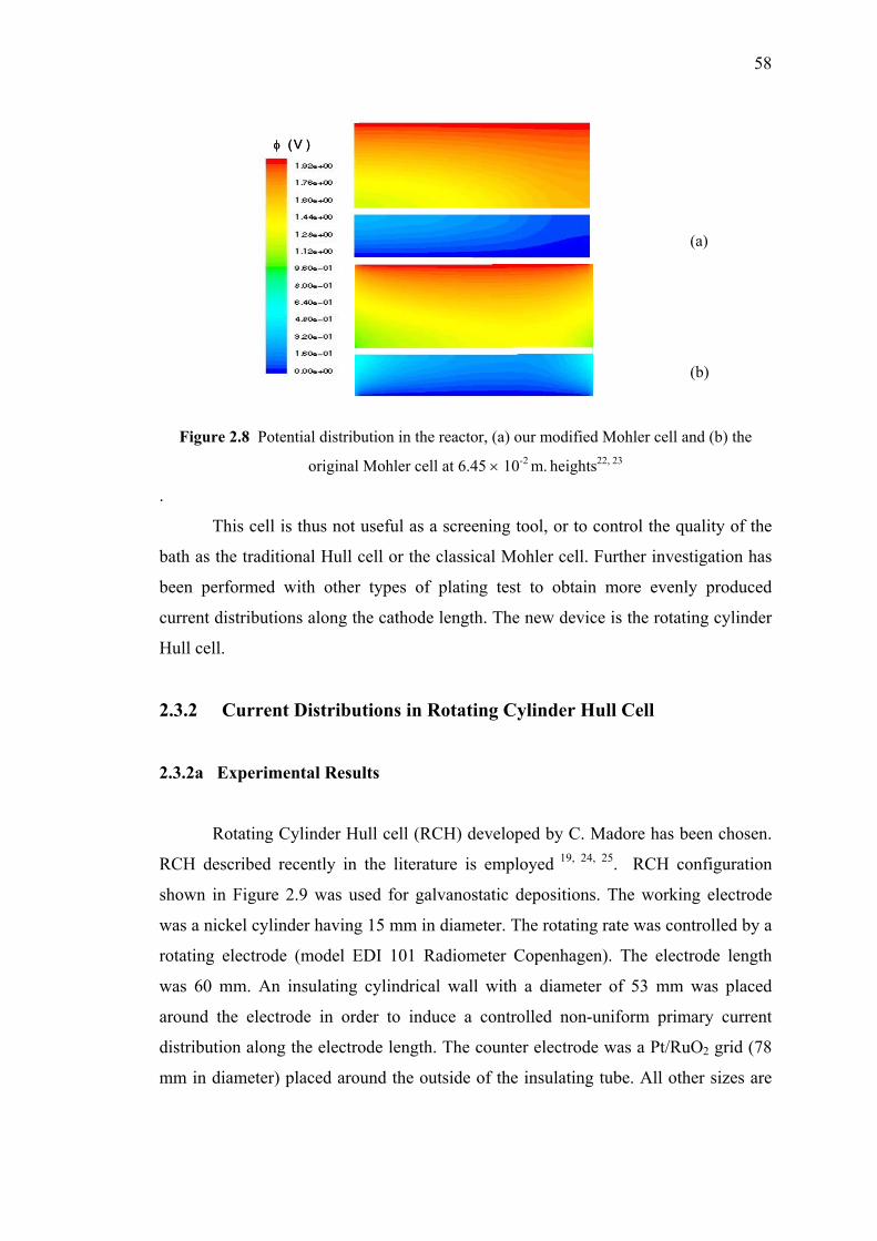
58

(a)

(b)

Figure 2.8 Potential distribution in the reactor, (a) our modified Mohler cell and (b) the

original Mohler cell at 6.45 × 10-2 m. heights22, 23

.

This cell is thus not useful as a screening tool, or to control the quality of the

bath as the traditional Hull cell or the classical Mohler cell. Further investigation has

been performed with other types of plating test to obtain more evenly produced

current distributions along the cathode length. The new device is the rotating cylinder

Hull cell.

2.3.2 Current Distributions in Rotating Cylinder Hull Cell

2.3.2a Experimental Results

Rotating Cylinder Hull cell (RCH) developed by C. Madore has been chosen.

RCH described recently in the literature is employed 19, 24, 25. RCH configuration

shown in Figure 2.9 was used for galvanostatic depositions. The working electrode

was a nickel cylinder having 15 mm in diameter. The rotating rate was controlled by a

rotating electrode (model EDI 101 Radiometer Copenhagen). The electrode length

was 60 mm. An insulating cylindrical wall with a diameter of 53 mm was placed

around the electrode in order to induce a controlled non-uniform primary current

distribution along the electrode length. The counter electrode was a Pt/RuO2 grid (78

mm in diameter) placed around the outside of the insulating tube. All other sizes are

φ (V )φ (V )

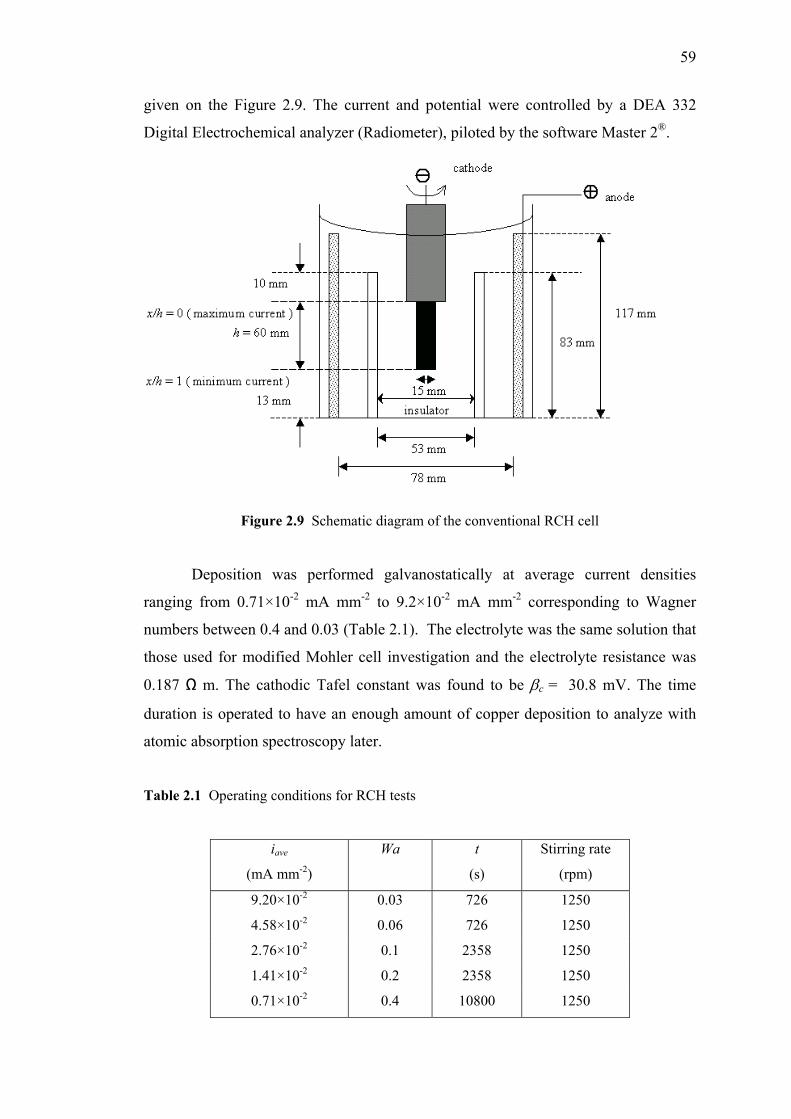
59

given on the Figure 2.9. The current and potential were controlled by a DEA 332

Digital Electrochemical analyzer (Radiometer), piloted by the software Master 2®.

Figure 2.9 Schematic diagram of the conventional RCH cell

Deposition was performed galvanostatically at average current densities

ranging from 0.71×10-2 mA mm-2 to 9.2×10-2 mA mm-2 corresponding to Wagner

numbers between 0.4 and 0.03 (Table 2.1). The electrolyte was the same solution that

those used for modified Mohler cell investigation and the electrolyte resistance was

0.187 Ω m. The cathodic Tafel constant was found to be βc = 30.8 mV. The time

duration is operated to have an enough amount of copper deposition to analyze with

atomic absorption spectroscopy later.

Table 2.1 Operating conditions for RCH tests

iave

(mA mm-2)

Wa

t

(s)

Stirring rate

(rpm)

9.20×10-2 0.03 726 1250

4.58×10-2 0.06 726 1250

2.76×10-2 0.1 2358 1250

1.41×10-2 0.2 2358 1250

0.71×10-2 0.4 10800 1250

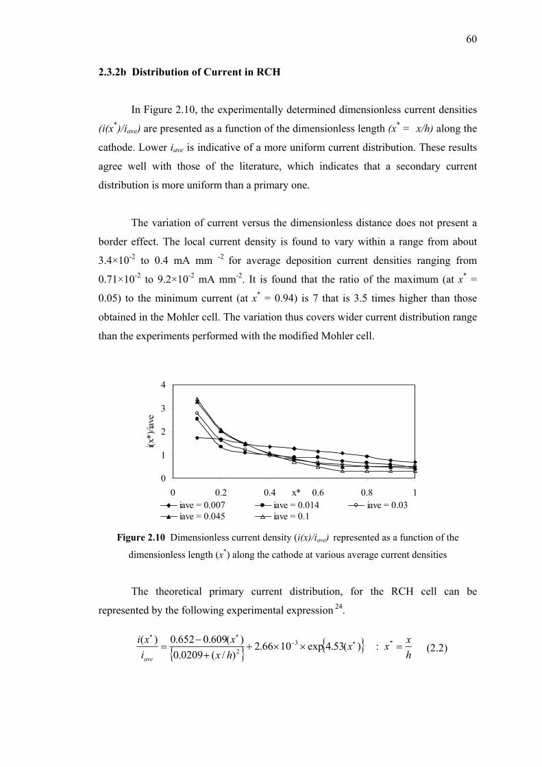
60

2.3.2b Distribution of Current in RCH

In Figure 2.10, the experimentally determined dimensionless current densities

(i(x*)/iave) are presented as a function of the dimensionless length (x* = x/h) along the

cathode. Lower iave is indicative of a more uniform current distribution. These results

agree well with those of the literature, which indicates that a secondary current

distribution is more uniform than a primary one.

The variation of current versus the dimensionless distance does not present a

border effect. The local current density is found to vary within a range from about

3.4×10-2 to 0.4 mA mm -2 for average deposition current densities ranging from

0.71×10-2 to 9.2×10-2 mA mm-2. It is found that the ratio of the maximum (at x* =

0.05) to the minimum current (at x* = 0.94) is 7 that is 3.5 times higher than those

obtained in the Mohler cell. The variation thus covers wider current distribution range

than the experiments performed with the modified Mohler cell.

0

1

2

3

4

0 0.2 0.4 0.6 0.8 1x*

i(x*)

/iave

iave = 0.007 iave = 0.014 iave = 0.03iave = 0.045 iave = 0.1

Figure 2.10 Dimensionless current density (i(x)/iave) represented as a function of the

dimensionless length (x*) along the cathode at various average current densities

The theoretical primary current distribution, for the RCH cell can be

represented by the following experimental expression 24.

(2.2)

hxxx

hxx

ixiave

=××++

−= ∗−

∗∗*3

2 :)(53.4exp1066.2)/(0209.0

)(609.0652.0)(

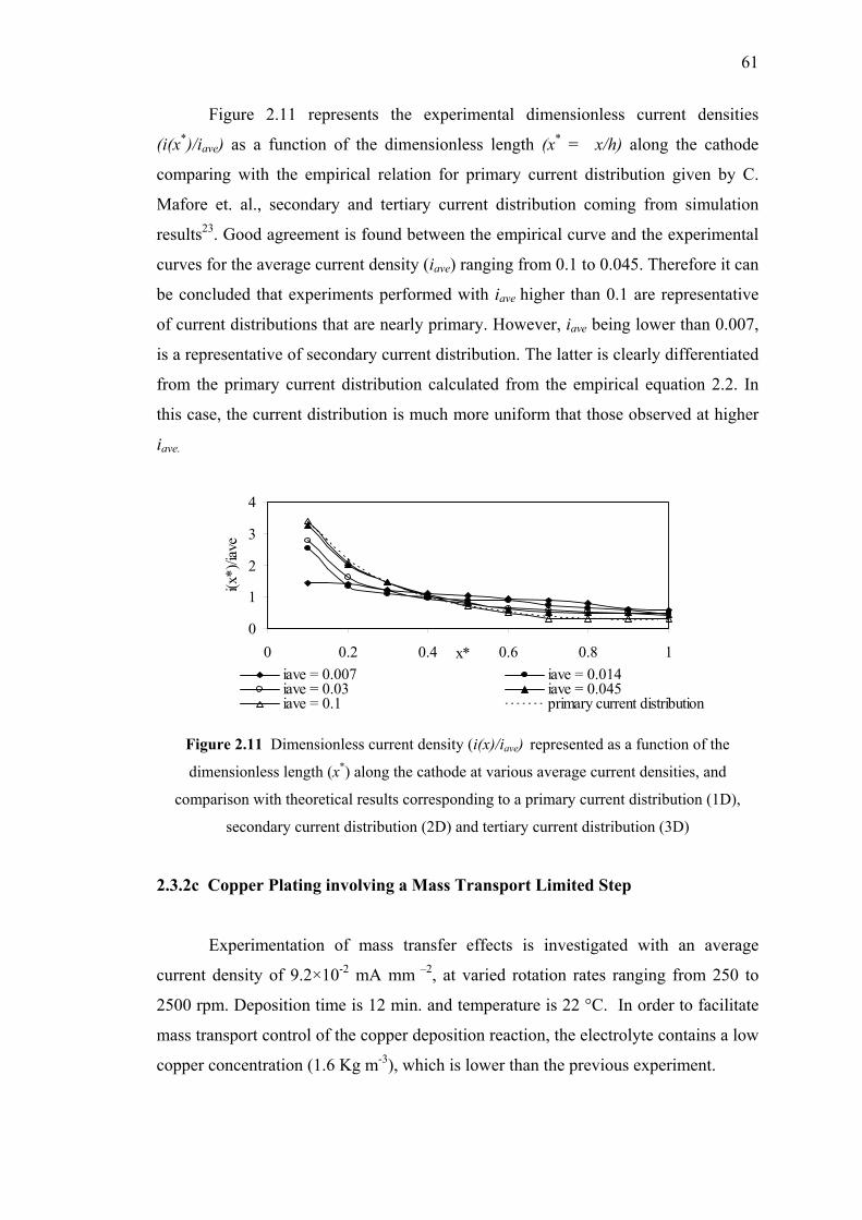
61

Figure 2.11 represents the experimental dimensionless current densities

(i(x*)/iave) as a function of the dimensionless length (x* = x/h) along the cathode

comparing with the empirical relation for primary current distribution given by C.

Mafore et. al., secondary and tertiary current distribution coming from simulation

results23. Good agreement is found between the empirical curve and the experimental

curves for the average current density (iave) ranging from 0.1 to 0.045. Therefore it can

be concluded that experiments performed with iave higher than 0.1 are representative

of current distributions that are nearly primary. However, iave being lower than 0.007,

is a representative of secondary current distribution. The latter is clearly differentiated

from the primary current distribution calculated from the empirical equation 2.2. In

this case, the current distribution is much more uniform that those observed at higher

iave.

0

1

2

3

4

0 0.2 0.4 0.6 0.8 1x*

i(x*)

/iave

iave = 0.007 iave = 0.014iave = 0.03 iave = 0.045iave = 0.1 primary current distribution

Figure 2.11 Dimensionless current density (i(x)/iave) represented as a function of the

dimensionless length (x*) along the cathode at various average current densities, and

comparison with theoretical results corresponding to a primary current distribution (1D),

secondary current distribution (2D) and tertiary current distribution (3D)

2.3.2c Copper Plating involving a Mass Transport Limited Step

Experimentation of mass transfer effects is investigated with an average

current density of 9.2×10-2 mA mm –2, at varied rotation rates ranging from 250 to

2500 rpm. Deposition time is 12 min. and temperature is 22 °C. In order to facilitate

mass transport control of the copper deposition reaction, the electrolyte contains a low

copper concentration (1.6 Kg m-3), which is lower than the previous experiment.

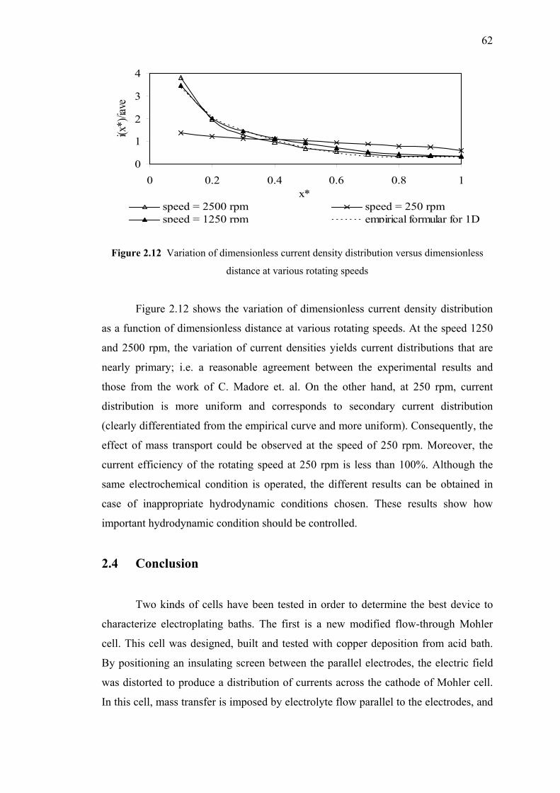
62

0

1

2

3

4

0 0.2 0.4 0.6 0.8 1x*

i(x*)

/iave

speed = 2500 rpm speed = 250 rpmspeed = 1250 rpm empirical formular for 1D

Figure 2.12 Variation of dimensionless current density distribution versus dimensionless

distance at various rotating speeds

Figure 2.12 shows the variation of dimensionless current density distribution

as a function of dimensionless distance at various rotating speeds. At the speed 1250

and 2500 rpm, the variation of current densities yields current distributions that are

nearly primary; i.e. a reasonable agreement between the experimental results and

those from the work of C. Madore et. al. On the other hand, at 250 rpm, current

distribution is more uniform and corresponds to secondary current distribution

(clearly differentiated from the empirical curve and more uniform). Consequently, the

effect of mass transport could be observed at the speed of 250 rpm. Moreover, the

current efficiency of the rotating speed at 250 rpm is less than 100%. Although the

same electrochemical condition is operated, the different results can be obtained in

case of inappropriate hydrodynamic conditions chosen. These results show how

important hydrodynamic condition should be controlled.

2.4 Conclusion

Two kinds of cells have been tested in order to determine the best device to

characterize electroplating baths. The first is a new modified flow-through Mohler

cell. This cell was designed, built and tested with copper deposition from acid bath.

By positioning an insulating screen between the parallel electrodes, the electric field

was distorted to produce a distribution of currents across the cathode of Mohler cell.

In this cell, mass transfer is imposed by electrolyte flow parallel to the electrodes, and

63

the experiments performed with this cell can be used to simulate electroplating under

industrial hydrodynamic conditions, especially for modern types of industrial cells

where mass transfer is imposed by circulation. Except for edge effects at the inlet and

outlet of the cathode, the ratio of the maximum to minimum current densities studied

was low, ranging from 1 to 2. This fact was confirmed by the results of a model

simulating a primary current distribution. However, it could be concluded that this

cell is not very useful as a bath control cell where a large range of current densities

must occur. The large area cathode allows study of the influence of current on the

deposit structure.

The second is a Rotating Cylinder Hull cell (RCH), which has been tested,

using the same electrolyte. It has been shown that experimental results agree well with

the empirical formula and theoretical results determined for primary current

distribution. In this case, the ratio of the maximum to the minimum current density (a

ratio of 7) covers wider range than those observed from the Mohler cell. It could be

concluded that this RCH cell constitutes an appropriate reactor to bath control.

Conclusion The current distribution is widely different in the reactor and significantly

relates to the composition. Accordingly, analysis of current distribution in the reactor

is an important factor in clarifying the composition, in relation to the current

distribution. The simulation study which is complicated and time consuming, was

performed by the research team. Basically, the mechanism model and its kinetic

parameters obtained from doing elemental experiments are solid foundations in

simulation study. The next part of this thesis therefore shows how the kinetic

parameters can be determined and how the mechanism model can be developed.

PART 3

MICROSCOPIC MODEL

Introduction

Increasing availability of computing power has made it possible to simulate

complex electrochemical phenomena. In addition, the design of complex substrate

geometry and the electroplating test cell have also been simulated. For example, the

simulation results for the current distribution of copper plating along the cathode

surface in Mohler cell and RCH cell have well corresponded to the experimental

observations in the part 2. For the simulation in the part 2, the simple mechanism and

kinetic constant are known with a certain boundary condition.

The mathematical model is not only the extremely useful tool to predict

physical event but also to process scale up or scale down, and to identify of

mechanisms as a guide to new complicate development of experiments such as alloy

plating, and prediction of the alloy composition from a minimum number of

experiments.

According to the part 2, the pieces of equipment controlling the bath

performance have been determined. In addition, the effects of current distributions

have been analyzed. The modeling of the electrochemical cell therefore could be

useful. The research team has done the simulation and model of the electrochemical

plating test cell. The data such as the boundary conditions, and kinetic parameters are

needed for completing the simulation. In the third chapter of this part is mentioned

how to determine these data.

The following concentrates on mathematical models predicting the

composition of electrodeposited binary alloys. The pure metal deposition is a simple

case study, while alloy deposition is more complicated and interesting. Zn-Ni alloy

deposition thus is investigated in the following study. The mechanism model of Zn-Ni

65

alloy is analyzed, and determined the kinetic parameters assuming a homogeneous

current distribution and mass transport rate on the working electrode. The established

model can be applied further for the computing simulation. The procedure is firstly

analyzed the behavior of the Zn-Ni alloy system according to the experimental part.

The following procedure is to determine the mechanism of Zn-Ni alloy and the kinetic

constant of the model.

The experiments to examine Zn-Ni alloy deposition depending on the

operation parameters have been carried out in order to hypothesize effectively the

mechanism model. The effect of complex agent to Zn-Ni alloy deposition has also

been studied.

Hence, the structure of this part follows by four main chapters.

Firstly, the bibliography relating to alloy plating, the literature reports of Zn-Ni alloy

deposition experiment, and of Zn-Ni alloy mechanisms have been reviewed.

Secondly, the experimental investigation of Zn-Ni alloy deposition has been carried

out. The microscopic model of Zn-Ni alloy deposition is followed as the third chapter.

The last one is thus the complex agent effect to Zn-Ni alloy deposition.

66

Chapter 1

Bibliography

1.1 Theoretical Aspect of Alloy Plating

1.1.1 Definition of Alloy

According to the metal handbooks, alloy can be defined as “ A substance that

has metallic properties and is composed of two or more chemical elements of which at

least one is a metal ” 27.

1.1.2 Plating Variable

The functional properties of electrodeposited alloys depend on their chemical

composition and on their structure in the micro and nano scales. Many factors could

affect the composition and microstructure of electrodeposited alloy as in Figure 1.1.

Figure 1.1 Factors influencing the composition and structure of electroplated alloys 13

Alloy Properties

Composition

Structure (micro, nano) Nucleation kinetic Growth kinetic Stress development Recrystallization Thermodynamics (phase diagram)

Electrode kinetic, adsorption Mass transport conditions Applied potential (current) Current (potential) distribution

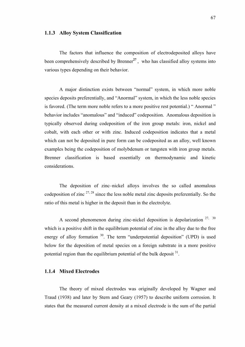
67

1.1.3 Alloy System Classification

The factors that influence the composition of electrodeposited alloys have

been comprehensively described by Brenner27 , who has classified alloy systems into

various types depending on their behavior.

A major distinction exists between “normal” system, in which more noble

species deposits preferentially, and “Anormal” system, in which the less noble species

is favored. (The term more noble refers to a more positive rest potential.) “ Anormal ”

behavior includes “anomalous” and “induced” codeposition. Anomalous deposition is

typically observed during codeposition of the iron group metals: iron, nickel and

cobalt, with each other or with zinc. Induced codeposition indicates that a metal

which can not be deposited in pure form can be codeposited as an alloy, well known

examples being the codeposition of molybdenum or tungsten with iron group metals.

Brenner classification is based essentially on thermodynamic and kinetic

considerations.

The deposition of zinc–nickel alloys involves the so called anomalous

codeposition of zinc 27, 28 since the less noble metal zinc deposits preferentially. So the

ratio of this metal is higher in the deposit than in the electrolyte.

A second phenomenon during zinc-nickel deposition is depolarization 27, 30

which is a positive shift in the equilibrium potential of zinc in the alloy due to the free

energy of alloy formation 30. The term “underpotential deposition” (UPD) is used

below for the deposition of metal species on a foreign substrate in a more positive

potential region than the equilibrium potential of the bulk deposit 31.

1.1.4 Mixed Electrodes

The theory of mixed electrodes was originally developed by Wagner and

Traud (1938) and later by Stern and Geary (1957) to describe uniform corrosion. It

states that the measured current density at a mixed electrode is the sum of the partial

68

current densities of all anodic and cathodic reactions (anodic partial current densities

are taken as positive value and cathodic partial current densities as negative one).

Normally, during alloy deposition, at least two electrochemical reactions

proceed simultaneously onto the cathode such as the deposition of the alloy

constituents and sometimes the formation of hydrogen. For deposition of a binary

alloy of metals A and B yields

i = iA + iB + iH2 (1.1)

where iA and iB are the partial current densities of alloy components A and B,

respectively, and iH is the current density for hydrogen formation. The current

efficiency for alloy deposition and the composition of the deposited alloy can be

expressed in terms of partial current densities. For deposition of a binary alloy AB,

this yields for the current efficiency, ε

iii BA +

=ε (1.2)

and for the alloy composition, xB (expressed as mole % of B)

100×+

=BBAA

BBB /ni/ni

/nix (1.3)

Here nA is the electron number involved in the deposition of component A of the

alloy, and nB for deposition of B. It follows from these equations that for given plating

conditions the composition of electrodeposited alloys and the current efficiency are

uniquely determined by the value of the partial current densities.

1.1.5 Variation of Alloy Compositions with Potential: Kinetic and

Thermodynamic Aspects

Figure 1.2 illustrates how the kinetics of partial reactions affects the

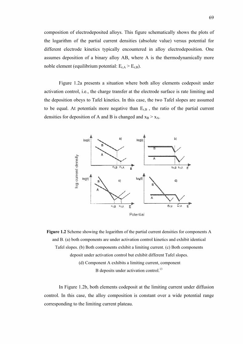
69

composition of electrodeposited alloys. This figure schematically shows the plots of

the logarithm of the partial current densities (absolute value) versus potential for

different electrode kinetics typically encountered in alloy electrodeposition. One

assumes deposition of a binary alloy AB, where A is the thermodynamically more

noble element (equilibrium potential: Er,A > Er,B).

Figure 1.2a presents a situation where both alloy elements codeposit under

activation control, i.e., the charge transfer at the electrode surface is rate limiting and

the deposition obeys to Tafel kinetics. In this case, the two Tafel slopes are assumed

to be equal. At potentials more negative than Er,B , the ratio of the partial current

densities for deposition of A and B is changed and xB > xA.

Figure 1.2 Scheme showing the logarithm of the partial current densities for components A

and B. (a) both components are under activation control kinetics and exhibit identical

Tafel slopes. (b) Both components exhibit a limiting current. (c) Both components

deposit under activation control but exhibit different Tafel slopes.

(d) Component A exhibits a limiting current, component

B deposits under activation control.13

In Figure 1.2b, both elements codeposit at the limiting current under diffusion

control. In this case, the alloy composition is constant over a wide potential range

corresponding to the limiting current plateau.

70

Figure 1.2c shows a situation where both elements codeposit under activation

control, but contrary to Figure 1.2a, here, the Tafel slope of element B is higher than

those of element A. The alloy composition therefore varies with potential. At not too

negative potentials, the partial current density of A dominates and the deposited alloy

contains mostly this element. On the other hand, at very negative potentials the partial

current density of B dominates and the alloy deposit therefore contains mostly B.

Note that over a wide potential range, the less noble element B deposits at a higher

rate than the more noble element A. In this case, the thermodynamic equilibrium

potential therefore gives no indication about the alloy composition resulting from

codeposition.

Figure 1.2d shows a situation where element A deposits under diffusion

control and B under activation control. At potentials more positive than the

equilibrium potential of B, only the more noble element A deposits, while at very

negative potentials, deposition of B dominates. The described situation is typical for

alloy plating electrolytes containing a noble element at low concentration and a less

noble element at high concentration.

1.1.6 Experimental Considerations: Determination of Partial Current

Densities

To study the codeposition behavior, we need to know how the partial current

densities vary with potential. Unfortunately partial current densities cannot be

measured directly. Their values must be calculated from the quantity and

composition of the deposited alloy. For example, for a binary alloy AB and a

thickness of deposit ∆d, the partial current density of B is

BB

BB m

tMFni∆

= (1.4)

Here, mB is the mass of element B deposited in the alloy, MB is the atomic weight of

element B, ∆t is the deposition time and nB is the number of electrons involved in the

71

reaction of element B. One can therefore estimate either the thickness by assuming

the density or the mass of the deposit.

Different chemical and physical methods are available for determining the

composition. This one can be obtained by chemical solution analysis after chemical

or electrochemical dissolution of the deposit or by physical methods such as X-ray

fluorescence (XRF). Electron microprobe analysis, microspot XRF, or scanning

Auger electron spectroscopy can also be used to determine the local and surface

composition of alloy deposits.

1.2 State of the Art on Experimental Investigation of Zn-Ni Alloy

Deposition

The use of zinc and its alloys for improving the corrosion resistance of coated

steel sheet has been growing worldwide. In the automotive industry, for example, its

use has been growing in a search to increase the corrosion resistance of chassis. In

recent years the interest in zinc alloy coatings, such Zn-Ni, Zn-Fe and Zn-Co, has

been increasing as a consequence of their better mechanical and anti-corrosion

properties than pure zinc coatings, and as a substitute for toxic and high cost

cadmium coatings. The Zn-Ni alloys obtained by electrodeposition processes, with

the amount of nickel varying between 8% and 14% by weight, give corrosion

protection five to six times superior to that obtained with pure zinc deposits32, 33.

Electrodepositions of zinc alloy in particular, Zn-Ni, are currently the subject of

many studies. They mainly concern sulfate or chloride bath33-36.

1.2.1 Zn-Ni Alloy Deposition from Acid and Alkaline Bath

1.2.1a Operating Conditions

The main Zn-Ni alloy processes are based on two types of electrolyte systems

as shown in Table 1.1. One acid type uses zinc and nickel salts (sulfate or chloride)

as the main source of metal ions in solution. The acid electrolyte contains buffering

agents, such as boric acid or acetic acid, to stabilize the pH during plating. Some

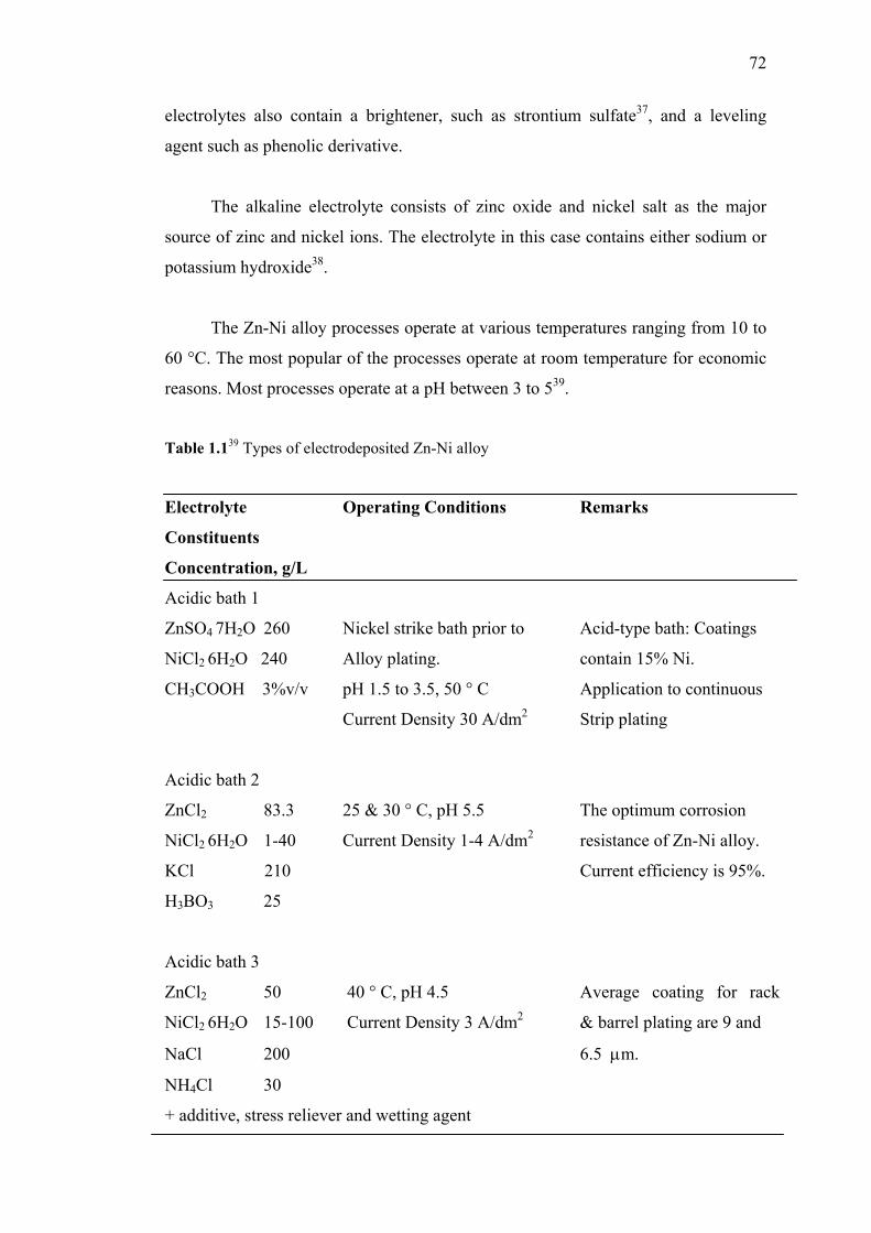
72

electrolytes also contain a brightener, such as strontium sulfate37, and a leveling

agent such as phenolic derivative.

The alkaline electrolyte consists of zinc oxide and nickel salt as the major

source of zinc and nickel ions. The electrolyte in this case contains either sodium or

potassium hydroxide38.

The Zn-Ni alloy processes operate at various temperatures ranging from 10 to

60 °C. The most popular of the processes operate at room temperature for economic

reasons. Most processes operate at a pH between 3 to 539.

Table 1.139 Types of electrodeposited Zn-Ni alloy

Electrolyte Operating Conditions Remarks

Constituents

Concentration, g/L

Acidic bath 1

ZnSO4 7H2O 260 Nickel strike bath prior to Acid-type bath: Coatings

NiCl2 6H2O 240 Alloy plating. contain 15% Ni.

CH3COOH 3%v/v pH 1.5 to 3.5, 50 ° C Application to continuous

Current Density 30 A/dm2 Strip plating

Acidic bath 2

ZnCl2 83.3 25 & 30 ° C, pH 5.5 The optimum corrosion

NiCl2 6H2O 1-40 Current Density 1-4 A/dm2 resistance of Zn-Ni alloy.

KCl 210 Current efficiency is 95%.

H3BO3 25

Acidic bath 3

ZnCl2 50 40 ° C, pH 4.5 Average coating for rack

NiCl2 6H2O 15-100 Current Density 3 A/dm2 & barrel plating are 9 and

NaCl 200 6.5 µm.

NH4Cl 30

+ additive, stress reliever and wetting agent

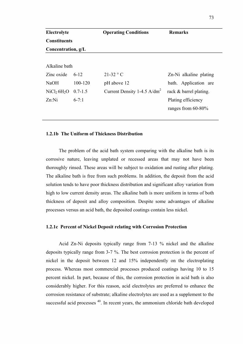
73

Electrolyte Operating Conditions Remarks

Constituents

Concentration, g/L

Alkaline bath

Zinc oxide 6-12 21-32 ° C Zn-Ni alkaline plating

NaOH 100-120 pH above 12 bath. Application are

NiCl2 6H2O 0.7-1.5 Current Density 1-4.5 A/dm2 rack & barrel plating.

Zn:Ni 6-7:1 Plating efficiency

ranges from 60-80%

1.2.1b The Uniform of Thickness Distribution

The problem of the acid bath system comparing with the alkaline bath is its

corrosive nature, leaving unplated or recessed areas that may not have been

thoroughly rinsed. These areas will be subject to oxidation and rusting after plating.

The alkaline bath is free from such problems. In addition, the deposit from the acid

solution tends to have poor thickness distribution and significant alloy variation from

high to low current density areas. The alkaline bath is more uniform in terms of both

thickness of deposit and alloy composition. Despite some advantages of alkaline

processes versus an acid bath, the deposited coatings contain less nickel.

1.2.1c Percent of Nickel Deposit relating with Corrosion Protection

Acid Zn-Ni deposits typically range from 7-13 % nickel and the alkaline

deposits typically range from 3-7 %. The best corrosion protection is the percent of

nickel in the deposit between 12 and 15% independently on the electroplating

process. Whereas most commercial processes produced coatings having 10 to 15

percent nickel. In part, because of this, the corrosion protection in acid bath is also

considerably higher. For this reason, acid electrolytes are preferred to enhance the

corrosion resistance of substrate; alkaline electrolytes are used as a supplement to the

successful acid processes 40. In recent years, the ammonium chloride bath developed

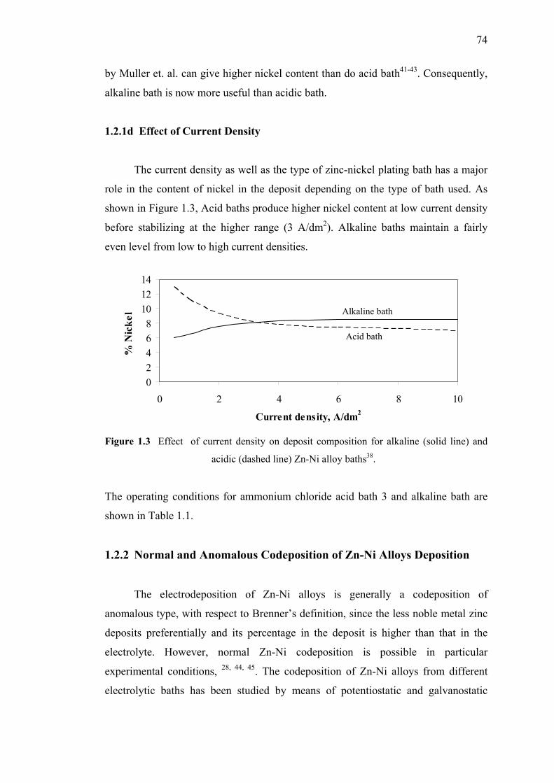
74

by Muller et. al. can give higher nickel content than do acid bath41-43. Consequently,

alkaline bath is now more useful than acidic bath.

1.2.1d Effect of Current Density

The current density as well as the type of zinc-nickel plating bath has a major

role in the content of nickel in the deposit depending on the type of bath used. As

shown in Figure 1.3, Acid baths produce higher nickel content at low current density

before stabilizing at the higher range (3 A/dm2). Alkaline baths maintain a fairly

even level from low to high current densities.

02468

101214

0 2 4 6 8 10

Current density, A/dm2

% N

icke

l

Figure 1.3 Effect of current density on deposit composition for alkaline (solid line) and

acidic (dashed line) Zn-Ni alloy baths38.

The operating conditions for ammonium chloride acid bath 3 and alkaline bath are

shown in Table 1.1.

1.2.2 Normal and Anomalous Codeposition of Zn-Ni Alloys Deposition

The electrodeposition of Zn-Ni alloys is generally a codeposition of

anomalous type, with respect to Brenner’s definition, since the less noble metal zinc

deposits preferentially and its percentage in the deposit is higher than that in the

electrolyte. However, normal Zn-Ni codeposition is possible in particular

experimental conditions, 28, 44, 45. The codeposition of Zn-Ni alloys from different

electrolytic baths has been studied by means of potentiostatic and galvanostatic

Alkaline bath

Acid bath

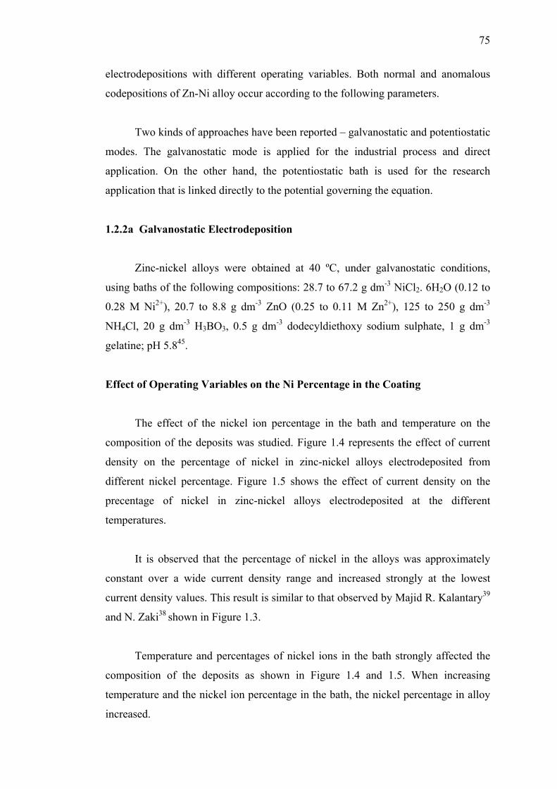
75

electrodepositions with different operating variables. Both normal and anomalous

codepositions of Zn-Ni alloy occur according to the following parameters.

Two kinds of approaches have been reported – galvanostatic and potentiostatic

modes. The galvanostatic mode is applied for the industrial process and direct

application. On the other hand, the potentiostatic bath is used for the research

application that is linked directly to the potential governing the equation.

1.2.2a Galvanostatic Electrodeposition

Zinc-nickel alloys were obtained at 40 ºC, under galvanostatic conditions,

using baths of the following compositions: 28.7 to 67.2 g dm-3 NiCl2. 6H2O (0.12 to

0.28 M Ni2+), 20.7 to 8.8 g dm-3 ZnO (0.25 to 0.11 M Zn2+), 125 to 250 g dm-3

NH4Cl, 20 g dm-3 H3BO3, 0.5 g dm-3 dodecyldiethoxy sodium sulphate, 1 g dm-3

gelatine; pH 5.845.

Effect of Operating Variables on the Ni Percentage in the Coating

The effect of the nickel ion percentage in the bath and temperature on the

composition of the deposits was studied. Figure 1.4 represents the effect of current

density on the percentage of nickel in zinc-nickel alloys electrodeposited from

different nickel percentage. Figure 1.5 shows the effect of current density on the

precentage of nickel in zinc-nickel alloys electrodeposited at the different

temperatures.

It is observed that the percentage of nickel in the alloys was approximately

constant over a wide current density range and increased strongly at the lowest

current density values. This result is similar to that observed by Majid R. Kalantary39

and N. Zaki38 shown in Figure 1.3.

Temperature and percentages of nickel ions in the bath strongly affected the

composition of the deposits as shown in Figure 1.4 and 1.5. When increasing

temperature and the nickel ion percentage in the bath, the nickel percentage in alloy

increased.

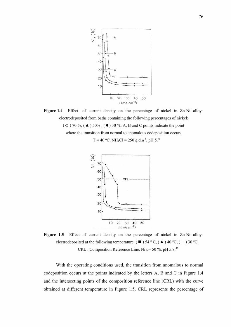
76

Figure 1.4 Effect of current density on the percentage of nickel in Zn-Ni alloys

electrodeposited from baths containing the following percentages of nickel:

( ) 70 %, ( ) 50% , ( ) 30 %. A, B and C points indicate the point

where the transition from normal to anomalous codeposition occurs.

T = 40 ºC, NH4Cl = 250 g dm-3, pH 5.45

Figure 1.5 Effect of current density on the percentage of nickel in Zn-Ni alloys

electrodeposited at the following temperature: ( ) 54 º C, ( ) 40 ºC, ( ) 30 ºC.

CRL : Composition Reference Line. Ni b = 50 %, pH 5.8.45

With the operating conditions used, the transition from anomalous to normal

codeposition occurs at the points indicated by the letters A, B and C in Figure 1.4

and the intersecting points of the composition reference line (CRL) with the curve

obtained at different temperature in Figure 1.5. CRL represents the percentage of

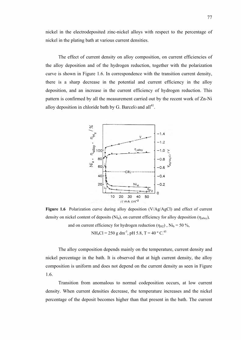
77

nickel in the electrodeposited zinc-nickel alloys with respect to the percentage of

nickel in the plating bath at various current densities.

The effect of current density on alloy composition, on current efficiencies of

the alloy deposition and of the hydrogen reduction, together with the polarization

curve is shown in Figure 1.6. In correspondence with the transition current density,

there is a sharp decrease in the potential and current efficiency in the alloy

deposition, and an increase in the current efficiency of hydrogen reduction. This

pattern is confirmed by all the measurement carried out by the recent work of Zn-Ni

alloy deposition in chloride bath by G. BarcelÒ and all41.

Figure 1.6 Polarization curve during alloy deposition (V/Ag/AgCl) and effect of current

density on nickel content of deposits (Nid), on current efficiency for alloy deposition (ηalloy),

and on current efficiency for hydrogen reduction (ηH2) , Nib = 50 %,

NH4Cl = 250 g dm-3, pH 5.8, T = 40 º C.45

The alloy composition depends mainly on the temperature, current density and

nickel percentage in the bath. It is observed that at high current density, the alloy

composition is uniform and does not depend on the current density as seen in Figure

1.6.

Transition from anomalous to normal codeposition occurs, at low current

density. When current densities decrease, the temperature increases and the nickel

percentage of the deposit becomes higher than that present in the bath. The current

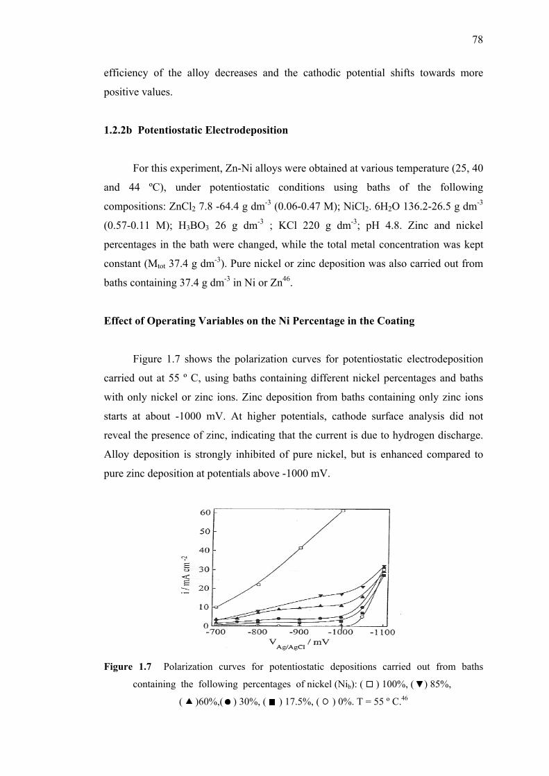
78

efficiency of the alloy decreases and the cathodic potential shifts towards more

positive values.

1.2.2b Potentiostatic Electrodeposition

For this experiment, Zn-Ni alloys were obtained at various temperature (25, 40

and 44 ºC), under potentiostatic conditions using baths of the following

compositions: ZnCl2 7.8 -64.4 g dm-3 (0.06-0.47 M); NiCl2. 6H2O 136.2-26.5 g dm-3

(0.57-0.11 M); H3BO3 26 g dm-3 ; KCl 220 g dm-3; pH 4.8. Zinc and nickel

percentages in the bath were changed, while the total metal concentration was kept

constant (Mtot 37.4 g dm-3). Pure nickel or zinc deposition was also carried out from

baths containing 37.4 g dm-3 in Ni or Zn46.

Effect of Operating Variables on the Ni Percentage in the Coating

Figure 1.7 shows the polarization curves for potentiostatic electrodeposition

carried out at 55 º C, using baths containing different nickel percentages and baths

with only nickel or zinc ions. Zinc deposition from baths containing only zinc ions

starts at about -1000 mV. At higher potentials, cathode surface analysis did not

reveal the presence of zinc, indicating that the current is due to hydrogen discharge.

Alloy deposition is strongly inhibited of pure nickel, but is enhanced compared to

pure zinc deposition at potentials above -1000 mV.

Figure 1.7 Polarization curves for potentiostatic depositions carried out from baths

containing the following percentages of nickel (Nib): ( ) 100%, ( ) 85%,

( )60%,( ) 30%, ( ) 17.5%, ( ) 0%. T = 55 º C.46

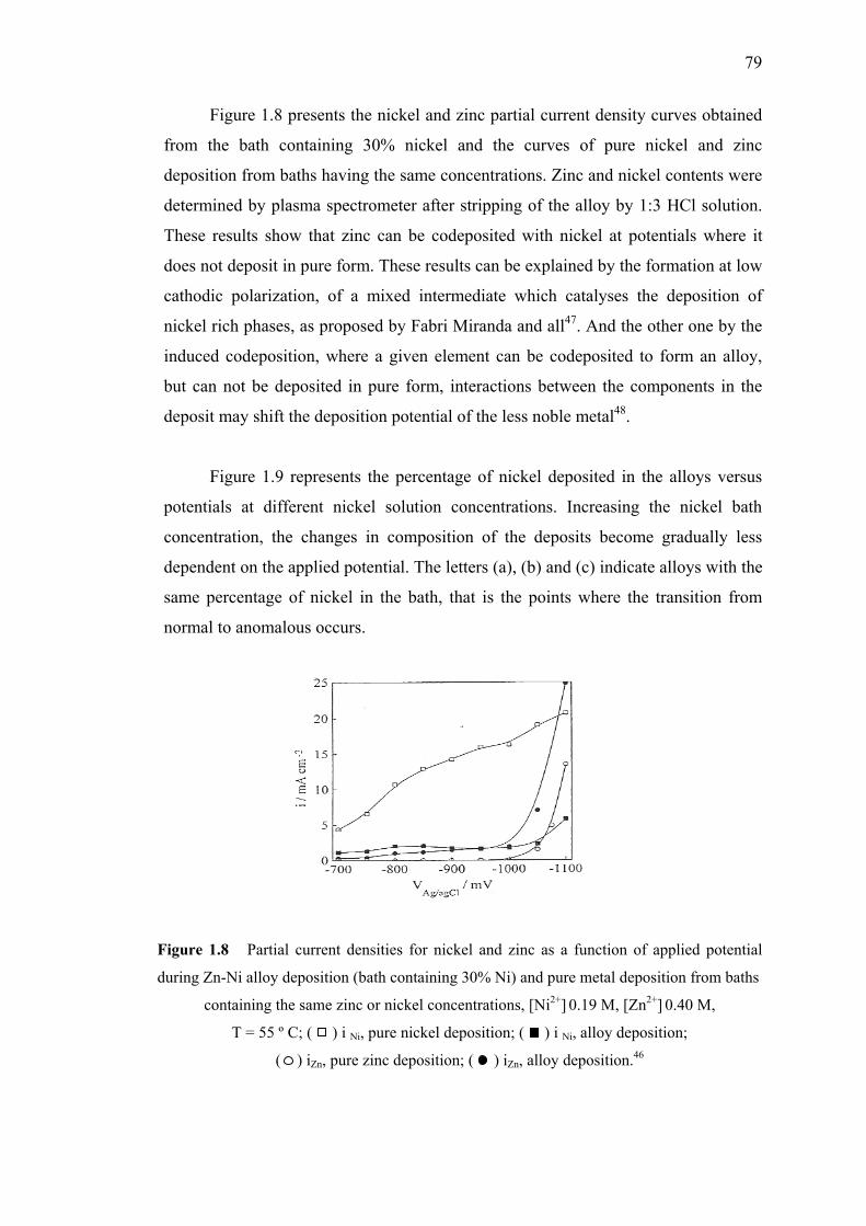
79

Figure 1.8 presents the nickel and zinc partial current density curves obtained

from the bath containing 30% nickel and the curves of pure nickel and zinc

deposition from baths having the same concentrations. Zinc and nickel contents were

determined by plasma spectrometer after stripping of the alloy by 1:3 HCl solution.

These results show that zinc can be codeposited with nickel at potentials where it

does not deposit in pure form. These results can be explained by the formation at low

cathodic polarization, of a mixed intermediate which catalyses the deposition of

nickel rich phases, as proposed by Fabri Miranda and all47. And the other one by the

induced codeposition, where a given element can be codeposited to form an alloy,

but can not be deposited in pure form, interactions between the components in the

deposit may shift the deposition potential of the less noble metal48.

Figure 1.9 represents the percentage of nickel deposited in the alloys versus

potentials at different nickel solution concentrations. Increasing the nickel bath

concentration, the changes in composition of the deposits become gradually less

dependent on the applied potential. The letters (a), (b) and (c) indicate alloys with the

same percentage of nickel in the bath, that is the points where the transition from

normal to anomalous occurs.

Figure 1.8 Partial current densities for nickel and zinc as a function of applied potential

during Zn-Ni alloy deposition (bath containing 30% Ni) and pure metal deposition from baths

containing the same zinc or nickel concentrations, [Ni2+] 0.19 M, [Zn2+] 0.40 M,

T = 55 º C; ( ) i Ni, pure nickel deposition; ( ) i Ni, alloy deposition;

( ) iZn, pure zinc deposition; ( ) iZn, alloy deposition.46

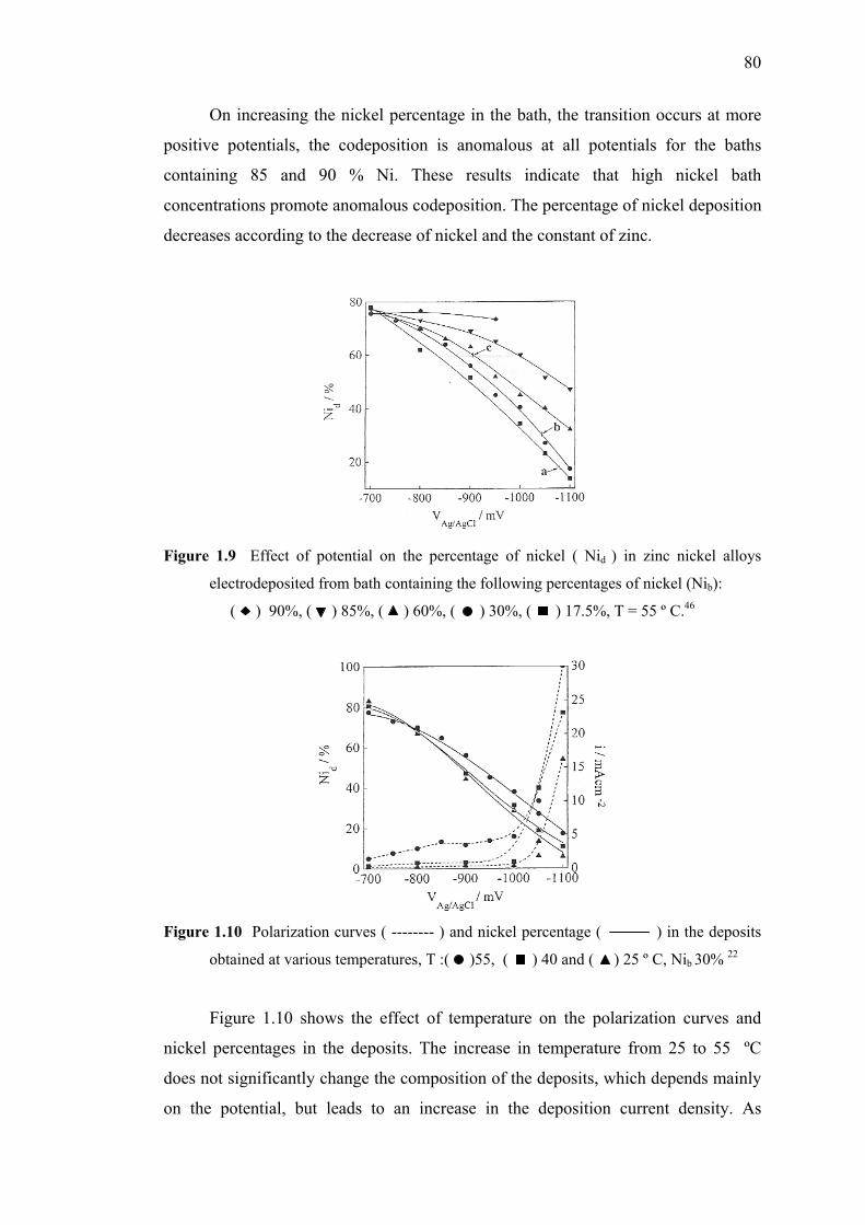
80

On increasing the nickel percentage in the bath, the transition occurs at more

positive potentials, the codeposition is anomalous at all potentials for the baths

containing 85 and 90 % Ni. These results indicate that high nickel bath

concentrations promote anomalous codeposition. The percentage of nickel deposition

decreases according to the decrease of nickel and the constant of zinc.

Figure 1.9 Effect of potential on the percentage of nickel ( Nid ) in zinc nickel alloys

electrodeposited from bath containing the following percentages of nickel (Nib):

( ) 90%, ( ) 85%, ( ) 60%, ( ) 30%, ( ) 17.5%, T = 55 º C.46

Figure 1.10 Polarization curves ( -------- ) and nickel percentage ( ) in the deposits

obtained at various temperatures, T :( )55, ( ) 40 and ( ) 25 º C, Nib 30% 22

Figure 1.10 shows the effect of temperature on the polarization curves and

nickel percentages in the deposits. The increase in temperature from 25 to 55 ºC

does not significantly change the composition of the deposits, which depends mainly

on the potential, but leads to an increase in the deposition current density. As

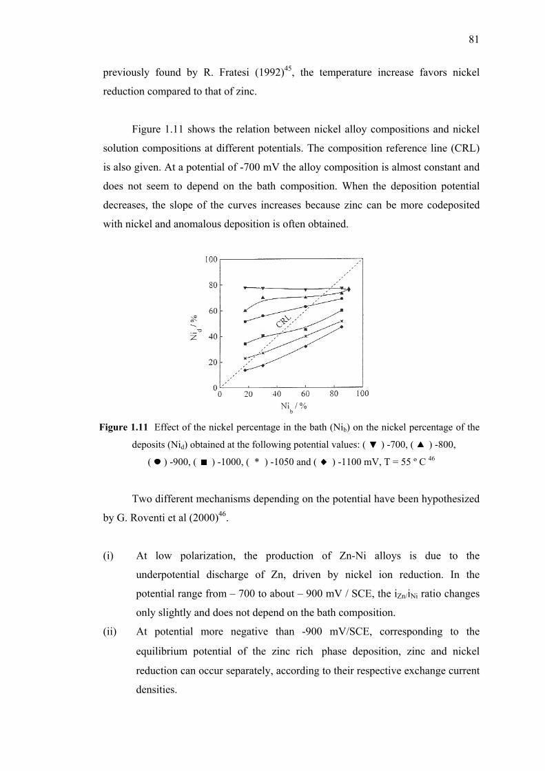
81

previously found by R. Fratesi (1992)45, the temperature increase favors nickel

reduction compared to that of zinc.

Figure 1.11 shows the relation between nickel alloy compositions and nickel

solution compositions at different potentials. The composition reference line (CRL)

is also given. At a potential of -700 mV the alloy composition is almost constant and

does not seem to depend on the bath composition. When the deposition potential

decreases, the slope of the curves increases because zinc can be more codeposited

with nickel and anomalous deposition is often obtained.

Figure 1.11 Effect of the nickel percentage in the bath (Nib) on the nickel percentage of the

deposits (Nid) obtained at the following potential values: ( ) -700, ( ) -800,

( ) -900, ( ) -1000, ( * ) -1050 and ( ) -1100 mV, T = 55 º C 46

Two different mechanisms depending on the potential have been hypothesized

by G. Roventi et al (2000)46.

(i) At low polarization, the production of Zn-Ni alloys is due to the

underpotential discharge of Zn, driven by nickel ion reduction. In the

potential range from – 700 to about – 900 mV / SCE, the iZn/iNi ratio changes

only slightly and does not depend on the bath composition.

(ii) At potential more negative than -900 mV/SCE, corresponding to the

equilibrium potential of the zinc rich phase deposition, zinc and nickel

reduction can occur separately, according to their respective exchange current

densities.

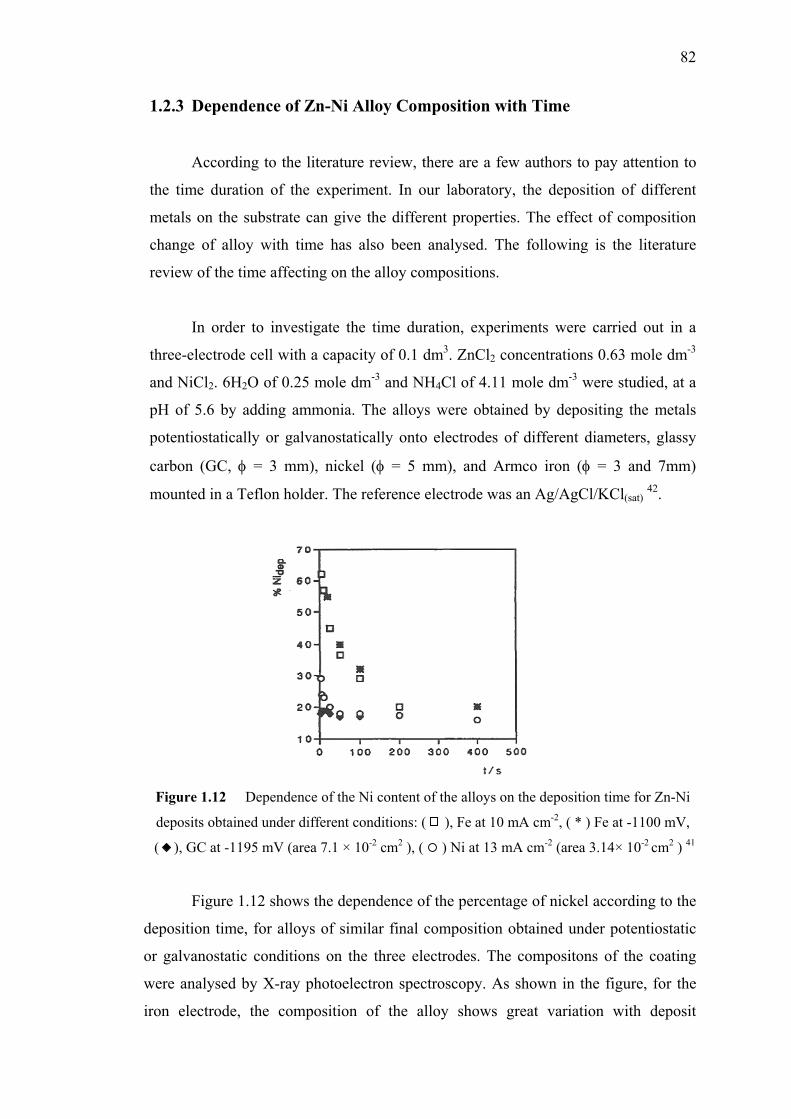
82

1.2.3 Dependence of Zn-Ni Alloy Composition with Time

According to the literature review, there are a few authors to pay attention to

the time duration of the experiment. In our laboratory, the deposition of different

metals on the substrate can give the different properties. The effect of composition

change of alloy with time has also been analysed. The following is the literature

review of the time affecting on the alloy compositions.

In order to investigate the time duration, experiments were carried out in a

three-electrode cell with a capacity of 0.1 dm3. ZnCl2 concentrations 0.63 mole dm-3

and NiCl2. 6H2O of 0.25 mole dm-3 and NH4Cl of 4.11 mole dm-3 were studied, at a

pH of 5.6 by adding ammonia. The alloys were obtained by depositing the metals

potentiostatically or galvanostatically onto electrodes of different diameters, glassy

carbon (GC, φ = 3 mm), nickel (φ = 5 mm), and Armco iron (φ = 3 and 7mm)

mounted in a Teflon holder. The reference electrode was an Ag/AgCl/KCl(sat) 42.

Figure 1.12 Dependence of the Ni content of the alloys on the deposition time for Zn-Ni

deposits obtained under different conditions: ( ), Fe at 10 mA cm-2, ( * ) Fe at -1100 mV,

( ), GC at -1195 mV (area 7.1 × 10-2 cm2 ), ( ) Ni at 13 mA cm-2 (area 3.14× 10-2 cm2 ) 41

Figure 1.12 shows the dependence of the percentage of nickel according to the

deposition time, for alloys of similar final composition obtained under potentiostatic

or galvanostatic conditions on the three electrodes. The compositons of the coating

were analysed by X-ray photoelectron spectroscopy. As shown in the figure, for the

iron electrode, the composition of the alloy shows great variation with deposit

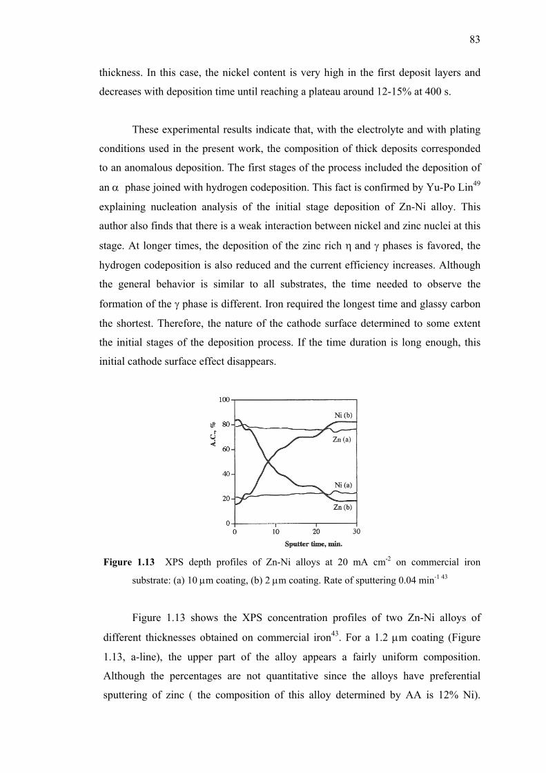
83

thickness. In this case, the nickel content is very high in the first deposit layers and

decreases with deposition time until reaching a plateau around 12-15% at 400 s.

These experimental results indicate that, with the electrolyte and with plating

conditions used in the present work, the composition of thick deposits corresponded

to an anomalous deposition. The first stages of the process included the deposition of

an α phase joined with hydrogen codeposition. This fact is confirmed by Yu-Po Lin49

explaining nucleation analysis of the initial stage deposition of Zn-Ni alloy. This

author also finds that there is a weak interaction between nickel and zinc nuclei at this

stage. At longer times, the deposition of the zinc rich η and γ phases is favored, the

hydrogen codeposition is also reduced and the current efficiency increases. Although

the general behavior is similar to all substrates, the time needed to observe the

formation of the γ phase is different. Iron required the longest time and glassy carbon

the shortest. Therefore, the nature of the cathode surface determined to some extent

the initial stages of the deposition process. If the time duration is long enough, this

initial cathode surface effect disappears.

Figure 1.13 XPS depth profiles of Zn-Ni alloys at 20 mA cm-2 on commercial iron

substrate: (a) 10 µm coating, (b) 2 µm coating. Rate of sputtering 0.04 min-1 43

Figure 1.13 shows the XPS concentration profiles of two Zn-Ni alloys of

different thicknesses obtained on commercial iron43. For a 1.2 µm coating (Figure

1.13, a-line), the upper part of the alloy appears a fairly uniform composition.

Although the percentages are not quantitative since the alloys have preferential

sputtering of zinc ( the composition of this alloy determined by AA is 12% Ni).

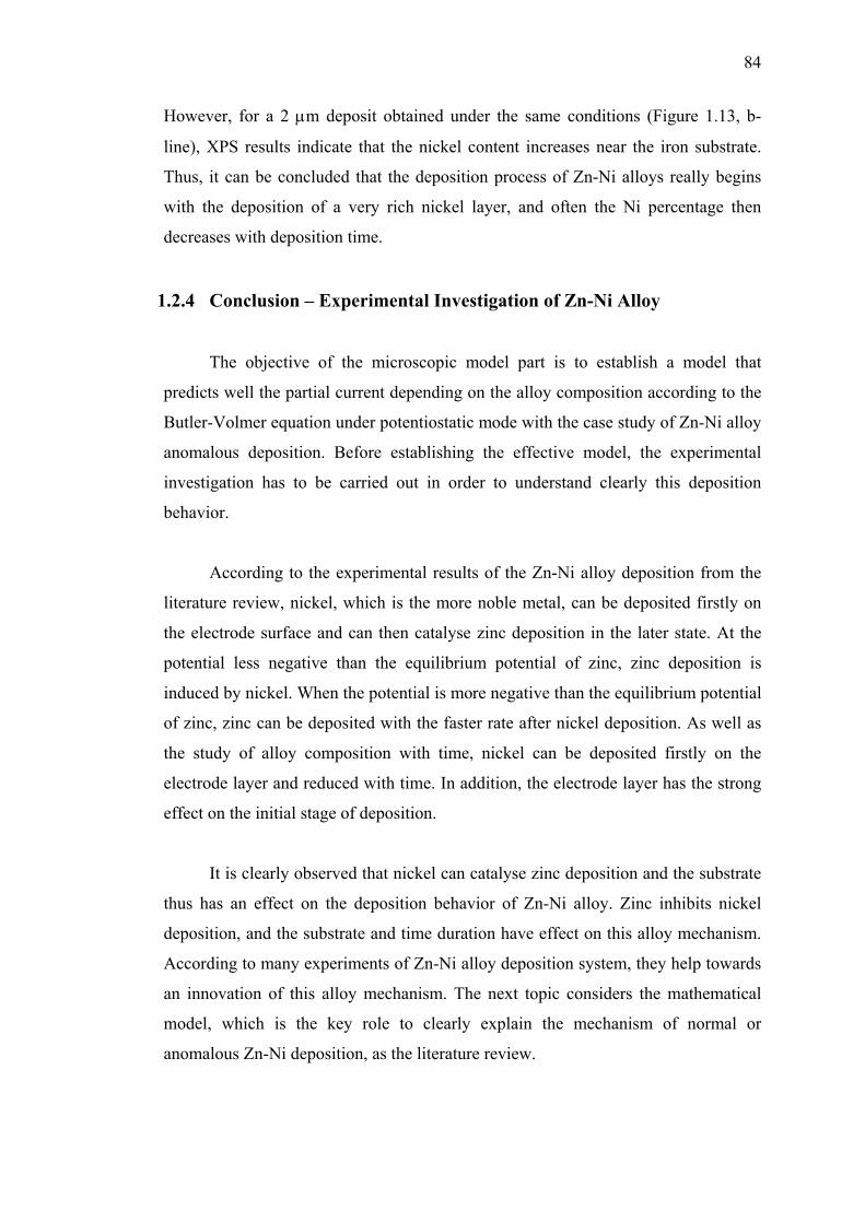
84

However, for a 2 µm deposit obtained under the same conditions (Figure 1.13, b-

line), XPS results indicate that the nickel content increases near the iron substrate.

Thus, it can be concluded that the deposition process of Zn-Ni alloys really begins

with the deposition of a very rich nickel layer, and often the Ni percentage then

decreases with deposition time.

1.2.4 Conclusion – Experimental Investigation of Zn-Ni Alloy

The objective of the microscopic model part is to establish a model that

predicts well the partial current depending on the alloy composition according to the

Butler-Volmer equation under potentiostatic mode with the case study of Zn-Ni alloy

anomalous deposition. Before establishing the effective model, the experimental

investigation has to be carried out in order to understand clearly this deposition

behavior.

According to the experimental results of the Zn-Ni alloy deposition from the

literature review, nickel, which is the more noble metal, can be deposited firstly on

the electrode surface and can then catalyse zinc deposition in the later state. At the

potential less negative than the equilibrium potential of zinc, zinc deposition is

induced by nickel. When the potential is more negative than the equilibrium potential

of zinc, zinc can be deposited with the faster rate after nickel deposition. As well as

the study of alloy composition with time, nickel can be deposited firstly on the

electrode layer and reduced with time. In addition, the electrode layer has the strong

effect on the initial stage of deposition.

It is clearly observed that nickel can catalyse zinc deposition and the substrate

thus has an effect on the deposition behavior of Zn-Ni alloy. Zinc inhibits nickel

deposition, and the substrate and time duration have effect on this alloy mechanism.

According to many experiments of Zn-Ni alloy deposition system, they help towards

an innovation of this alloy mechanism. The next topic considers the mathematical

model, which is the key role to clearly explain the mechanism of normal or

anomalous Zn-Ni deposition, as the literature review.

85

1.3 Mathematical Modeling investigation of Zn-Ni Alloy Deposition

Electrodeposition of binary alloys of the iron group metals exhibits anomalous

codeposition, which the less noble metal electrodeposits preferentially, as stated by

Brenner27. Anomalous behavior for binary systems is most often associated with the

mutual codeposition of the iron group metal (Fe, Ni or Co) and zinc or cadmium. In

the system of Zn-Ni alloy and Fe-Ni alloy are normally the anomalous deposition

behavior.

Many authors have studied the mechanism of anomalous codeposition of iron

group metals and several hypotheses have been presented, but there is still no theory

universally accepted. By this research, two models, the hydroxide suppression

mechanism model and the property interface model, are categorized from many

models of literature review.

1.3.1 Mechanism Involving Hydroxide Species

1.3.1a Hydroxide Suppression Mechanism [H. Dahms and I. M. Croll, 1965]50

This model assumes the dependence of the anomalous codeposition of iron-

nickel alloys on the pH at the cathode surface is investigated. An equation is derived

to evaluate the surface pH as a function of bulk pH, rate of hydrogen evolution, buffer

concentration, and diffusion mass conditions. The experimental results obtained on

rotating disk electrodes show that anomalous codeposition is due to a suppression of

nickel discharge and that suppression occurs only when the surface pH is high enough

to cause hydroxide formation. They concluded that the increased hydroxide ion

concentration near the surface should lead to the formation of ferrous hydroxide,

which is adsorbed further on the cathode and suppresses the deposition of nickel and

permits a high discharge rate of Fe2+. The mechanism is proposed by which the

adsorption of ferrous hydroxide suppresses the deposition of nickel, but permits a

high rate of iron discharge.

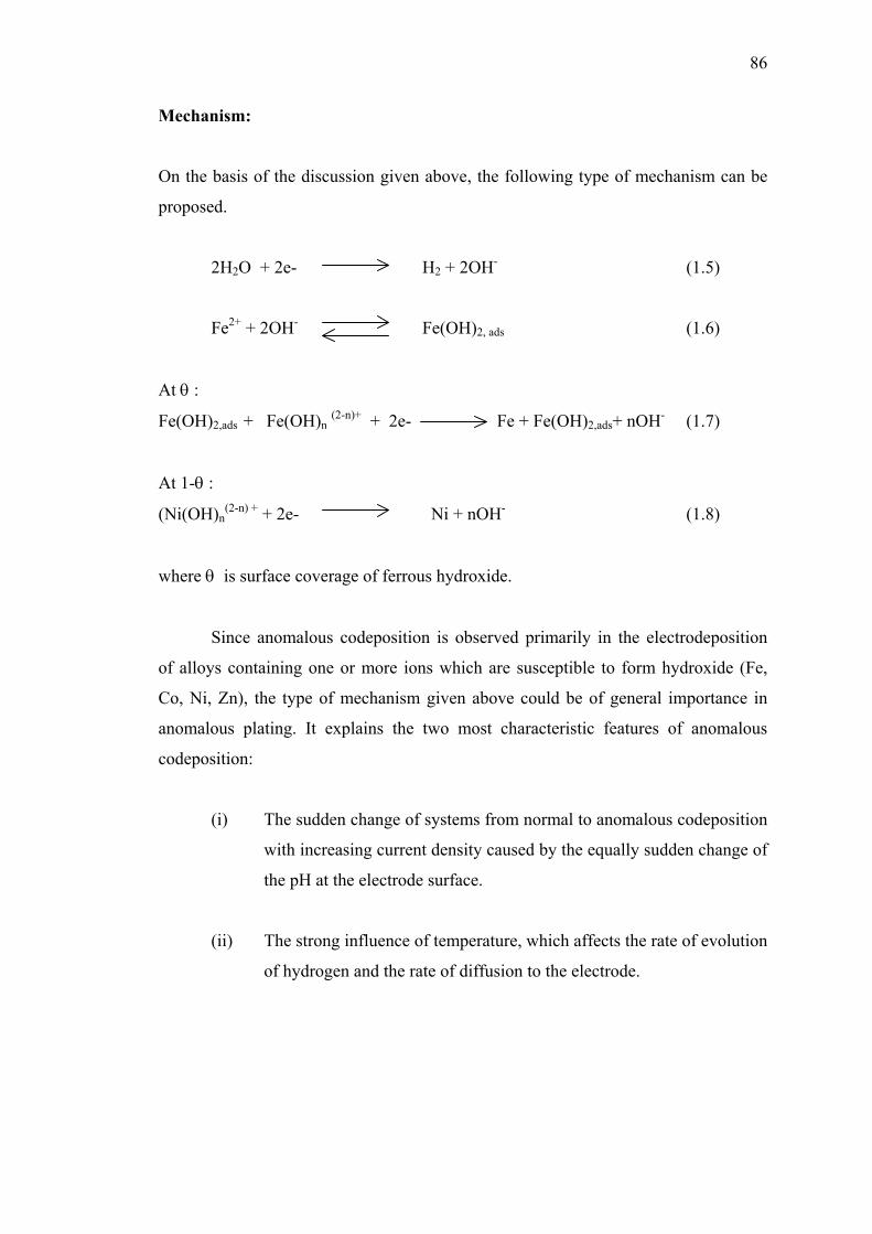
86

Mechanism:

On the basis of the discussion given above, the following type of mechanism can be

proposed.

2H2O + 2e- H2 + 2OH- (1.5)

Fe2+ + 2OH- Fe(OH)2, ads (1.6)

At θ :

Fe(OH)2,ads + Fe(OH)n (2-n)+ + 2e- Fe + Fe(OH)2,ads+ nOH- (1.7)

At 1-θ :

(Ni(OH)n(2-n) + + 2e- Ni + nOH- (1.8)

where θ is surface coverage of ferrous hydroxide.

Since anomalous codeposition is observed primarily in the electrodeposition

of alloys containing one or more ions which are susceptible to form hydroxide (Fe,

Co, Ni, Zn), the type of mechanism given above could be of general importance in

anomalous plating. It explains the two most characteristic features of anomalous

codeposition:

(i) The sudden change of systems from normal to anomalous codeposition

with increasing current density caused by the equally sudden change of

the pH at the electrode surface.

(ii) The strong influence of temperature, which affects the rate of evolution

of hydrogen and the rate of diffusion to the electrode.

87

The Model Disadvantages:

- A large pH rise is not a prerequisite for anomalous codeposition 51-55

due to the fact that such anomalous codeposition could also be

observed for low pH. This agrees with several authors.

- This theory does not explain the enhancement of zinc reduction

observed in the normal deposition region, the high current efficiency

during anomalous codeposition and the increase in nickel content in

the alloy with increasing pH 35.

According to above disadvantages, this model is not taken into account for

developing Zn-Ni alloy mechanism. Other mechanisms involving hydroxide species

are those proposed by Wendy C. Grande and Jan B. Talbot.

1.3.1b The pH Dependent Competitive Adsorption of Monohydroxide Species,

MOH+ [Wendy C. Grande and Jan B. Talbot, 1993]53

According to the explanation of anomalous mechanism was proposed by

Dahms and Croll, their experimental results suggested that the onset of anomalous

codeposition coincided with a rise in surface pH due to simultaneous hydrogen

evolution and alloy deposition at the cathode. They concluded that the increased

hydroxide ion concentration near the surface should lead to the formation of ferrous

hydroxide which, when adsorbed on the cathode, suppresses the deposition of nickel

and permits a high discharge rate of Fe2+. Recently, experimental results56-58 and

mathematical modeling51, 58 of nickel-iron deposition have shown anomalous

behavior even at low hydrogen evolution rates, these studies suggest that a rise in

surface pH is not necessarily required for anomalous codeposition to occur.

In this study, a mathematical model is developed to describe the codeposition

of nickel and iron in a simple sulfate solution. The approach to analyze anomalous

codeposition of Ni-Fe is comprised of two parts:

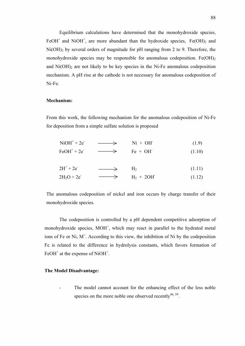
88

Equilibrium calculations have determined that the monohydroxide species,

FeOH+ and NiOH+, are more abundant than the hydroxide species, Fe(OH)2 and

Ni(OH)2 by several orders of magnitude for pH ranging from 2 to 9. Therefore, the

monohydroxide species may be responsible for anomalous codeposition. Fe(OH)2

and Ni(OH)2 are not likely to be key species in the Ni-Fe anomalous codeposition

mechanism. A pH rise at the cathode is not necessary for anomalous codeposition of

Ni-Fe.

Mechanism:

From this work, the following mechanism for the anomalous codeposition of Ni-Fe

for deposition from a simple sulfate solution is proposed

NiOH+ + 2e- Ni + OH- (1.9)

FeOH+ + 2e- Fe + OH- (1.10)

2H+ + 2e- H2 (1.11)

2H2O + 2e- H2 + 2OH- (1.12)

The anomalous codeposition of nickel and iron occurs by charge transfer of their

monohydroxide species.

The codeposition is controlled by a pH dependent competitive adsorption of

monohydroxide species, MOH+, which may react in parallel to the hydrated metal

ions of Fe or Ni, M+. According to this view, the inhibition of Ni by the codeposition

Fe is related to the difference in hydrolysis constants, which favors formation of

FeOH+ at the expense of NiOH+.

The Model Disadvantage:

- The model cannot account for the enhancing effect of the less noble

species on the more noble one observed recently46, 59.

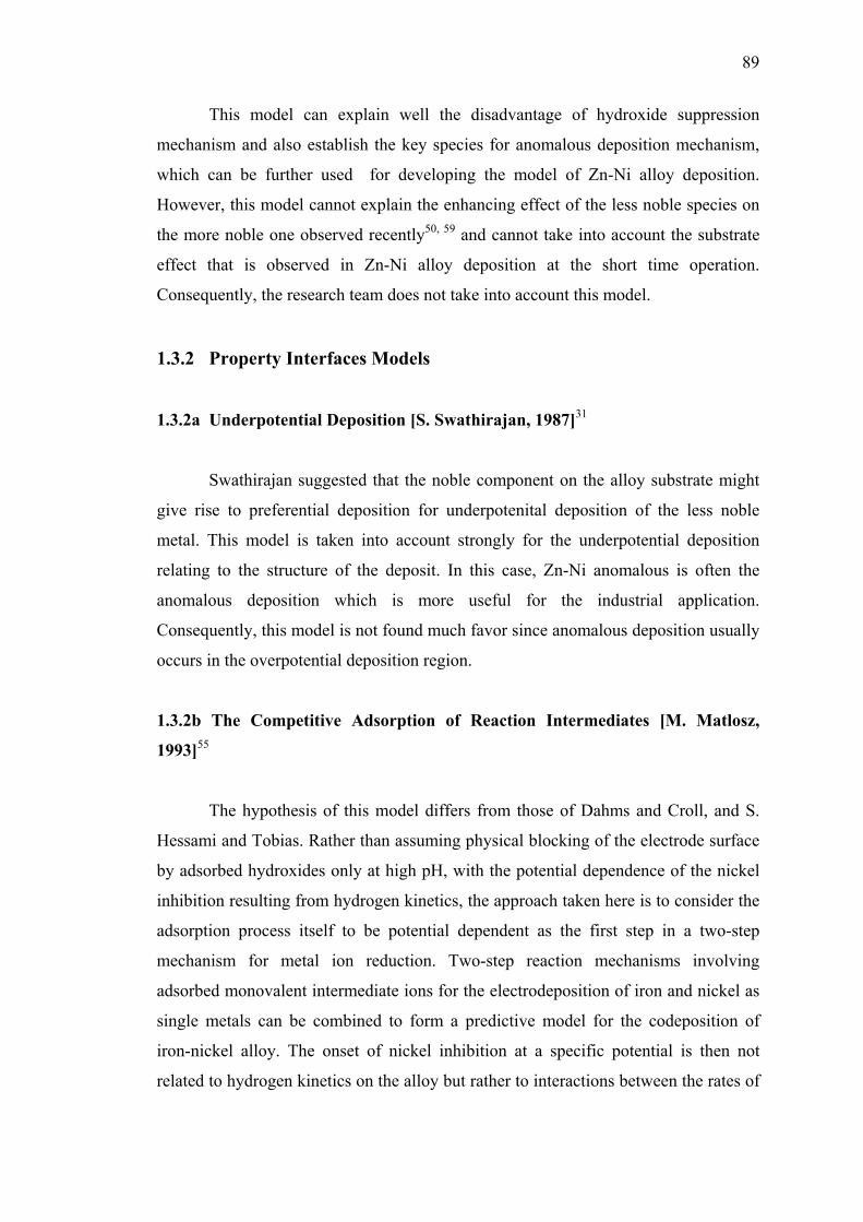
89

This model can explain well the disadvantage of hydroxide suppression

mechanism and also establish the key species for anomalous deposition mechanism,

which can be further used for developing the model of Zn-Ni alloy deposition.

However, this model cannot explain the enhancing effect of the less noble species on

the more noble one observed recently50, 59 and cannot take into account the substrate

effect that is observed in Zn-Ni alloy deposition at the short time operation.

Consequently, the research team does not take into account this model.

1.3.2 Property Interfaces Models

1.3.2a Underpotential Deposition [S. Swathirajan, 1987]31

Swathirajan suggested that the noble component on the alloy substrate might

give rise to preferential deposition for underpotenital deposition of the less noble

metal. This model is taken into account strongly for the underpotential deposition

relating to the structure of the deposit. In this case, Zn-Ni anomalous is often the

anomalous deposition which is more useful for the industrial application.

Consequently, this model is not found much favor since anomalous deposition usually

occurs in the overpotential deposition region.

1.3.2b The Competitive Adsorption of Reaction Intermediates [M. Matlosz,

1993]55

The hypothesis of this model differs from those of Dahms and Croll, and S.

Hessami and Tobias. Rather than assuming physical blocking of the electrode surface

by adsorbed hydroxides only at high pH, with the potential dependence of the nickel

inhibition resulting from hydrogen kinetics, the approach taken here is to consider the

adsorption process itself to be potential dependent as the first step in a two-step

mechanism for metal ion reduction. Two-step reaction mechanisms involving

adsorbed monovalent intermediate ions for the electrodeposition of iron and nickel as

single metals can be combined to form a predictive model for the codeposition of

iron-nickel alloy. The onset of nickel inhibition at a specific potential is then not

related to hydrogen kinetics on the alloy but rather to interactions between the rates of

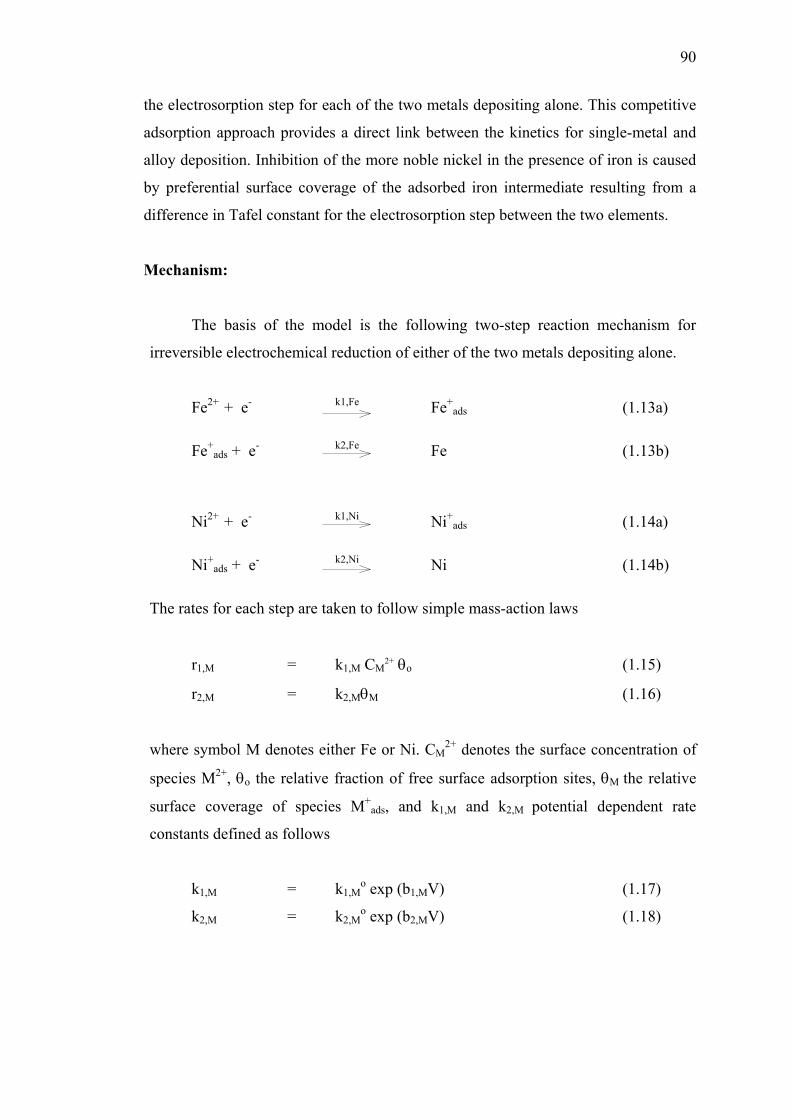
90

the electrosorption step for each of the two metals depositing alone. This competitive

adsorption approach provides a direct link between the kinetics for single-metal and

alloy deposition. Inhibition of the more noble nickel in the presence of iron is caused

by preferential surface coverage of the adsorbed iron intermediate resulting from a

difference in Tafel constant for the electrosorption step between the two elements.

Mechanism:

The basis of the model is the following two-step reaction mechanism for

irreversible electrochemical reduction of either of the two metals depositing alone.

Fe2+ + e- k1,Fe Fe+ads (1.13a)

Fe+ads + e- k2,Fe Fe (1.13b)

Ni2+ + e- k1,Ni Ni+ads (1.14a)

Ni+ads + e- k2,Ni Ni (1.14b)

The rates for each step are taken to follow simple mass-action laws

r1,M = k1,M CM2+ θo (1.15)

r2,M = k2,MθM (1.16)

where symbol M denotes either Fe or Ni. CM2+ denotes the surface concentration of

species M2+, θo the relative fraction of free surface adsorption sites, θM the relative

surface coverage of species M+ads, and k1,M and k2,M potential dependent rate

constants defined as follows

k1,M = k1,Mo exp (b1,MV) (1.17)

k2,M = k2,Mo exp (b2,MV) (1.18)

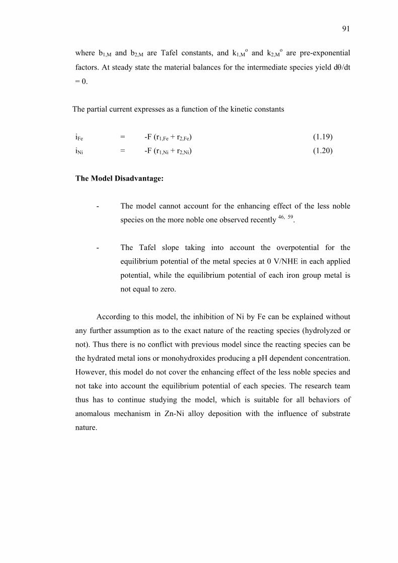
91

where b1,M and b2,M are Tafel constants, and k1,Mo and k2,M

o are pre-exponential

factors. At steady state the material balances for the intermediate species yield dθ/dt

= 0.

The partial current expresses as a function of the kinetic constants

iFe = -F (r1,Fe + r2,Fe) (1.19)

iNi = -F (r1,Ni + r2,Ni) (1.20)

The Model Disadvantage:

- The model cannot account for the enhancing effect of the less noble

species on the more noble one observed recently 46, 59.

- The Tafel slope taking into account the overpotential for the

equilibrium potential of the metal species at 0 V/NHE in each applied

potential, while the equilibrium potential of each iron group metal is

not equal to zero.

According to this model, the inhibition of Ni by Fe can be explained without

any further assumption as to the exact nature of the reacting species (hydrolyzed or

not). Thus there is no conflict with previous model since the reacting species can be

the hydrated metal ions or monohydroxides producing a pH dependent concentration.

However, this model do not cover the enhancing effect of the less noble species and

not take into account the equilibrium potential of each species. The research team

thus has to continue studying the model, which is suitable for all behaviors of

anomalous mechanism in Zn-Ni alloy deposition with the influence of substrate

nature.

92

1.3.2c An Adsorbed Mixed Reaction Intermediate containing the Two

Codepositing Species in Partly Reduced Form [ N. Zech, E.J. Podlaha and D.

Landolt, 1999]59 and [E. Chassiang and R. Wiart ]60

The different models proposed further in the literature can explain the

observed inhibition of Ni by Fe, but they cannot account for the enhancing effect of

the less noble species on the more noble one observed recently by G. Roventi et al46

and N. Zech59. In this model, anomalous deposition model is presented and critically

evaluated which includes both inhibiting effects and enhancing effects. The model

assumes that the controlling mechanism for both inhibiting and enhancement

involves the formation of an adsorbed mixed reaction intermediate containing the

two codepositing species in partly reduced from.

A mathematical model for anomalous codeposition of iron group metals is

presented which describes effects of inhibition and enhancement observed

experimentally during codeposition of Fe-Ni alloy. The model assumes three parallel

reaction paths, each one proceeding in two consecutive steps, and takes into account

the effect of mass transport. The model assumes that deposition involved an adsorbed

reaction intermediate containing both metal ions in partly reduced form. This

reaction intermediate is responsible for both the inhibition of the more noble species

and the enhancement of the less noble species.

Mechanism

The present model is based on the assumption that both single metals are reduced in

two consecutive steps, as described by Matlosz55.

Fe2+ + e- k11 Fe+ads (1.25a)

Fe+ads + e- k12 Fe(s) (1.25b)

Ni2+ + e- k21 Ni+ads (1.26a)

Ni+ads + e- k22 Ni(s) (1.26b)

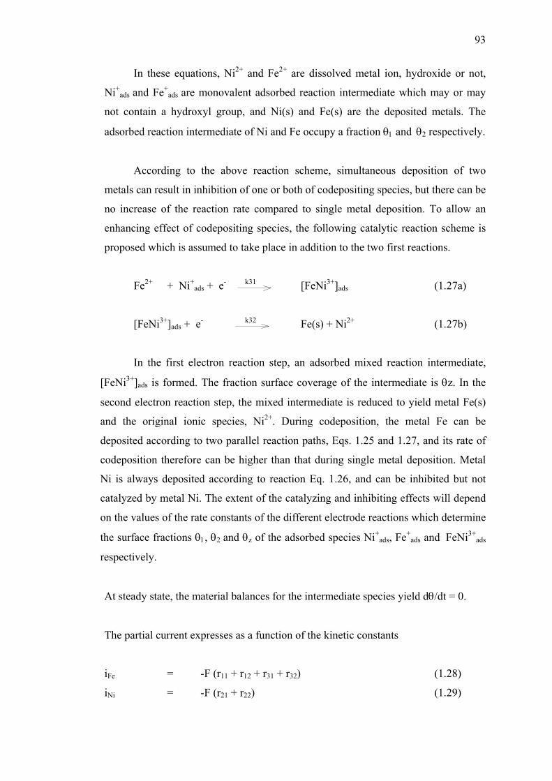
93

In these equations, Ni2+ and Fe2+ are dissolved metal ion, hydroxide or not,

Ni+ads and Fe+

ads are monovalent adsorbed reaction intermediate which may or may

not contain a hydroxyl group, and Ni(s) and Fe(s) are the deposited metals. The

adsorbed reaction intermediate of Ni and Fe occupy a fraction θ1 and θ2 respectively.

According to the above reaction scheme, simultaneous deposition of two

metals can result in inhibition of one or both of codepositing species, but there can be

no increase of the reaction rate compared to single metal deposition. To allow an

enhancing effect of codepositing species, the following catalytic reaction scheme is

proposed which is assumed to take place in addition to the two first reactions.

Fe2+ + Ni+ads + e- k31 [FeNi3+]ads (1.27a)

[FeNi3+]ads + e- k32 Fe(s) + Ni2+ (1.27b)

In the first electron reaction step, an adsorbed mixed reaction intermediate,

[FeNi3+]ads is formed. The fraction surface coverage of the intermediate is θz. In the

second electron reaction step, the mixed intermediate is reduced to yield metal Fe(s)

and the original ionic species, Ni2+. During codeposition, the metal Fe can be

deposited according to two parallel reaction paths, Eqs. 1.25 and 1.27, and its rate of

codeposition therefore can be higher than that during single metal deposition. Metal

Ni is always deposited according to reaction Eq. 1.26, and can be inhibited but not

catalyzed by metal Ni. The extent of the catalyzing and inhibiting effects will depend

on the values of the rate constants of the different electrode reactions which determine

the surface fractions θ1, θ2 and θz of the adsorbed species Ni+ads, Fe+

ads and FeNi3+ads

respectively.

At steady state, the material balances for the intermediate species yield dθ/dt = 0.

The partial current expresses as a function of the kinetic constants

iFe = -F (r11 + r12 + r31 + r32) (1.28)

iNi = -F (r21 + r22) (1.29)

94

The Model Disadvantage

- The Tafel slope taking into account the overpotential for the

equilibrium potential of the metal species at 0 V/MSE in each applied

potentials, while the equilibrium potential of each metals in iron group

metal is not equal to zero.

- The kinetic parameters for the mixed-intermediate reaction pathway

can only be obtained from the experimental data of alloy deposition.

Therefore, the model does not permit a prediction of anomalous

codeposition behavior in case of single metal kinetics.

- The model cannot be used for the quantitative prediction of the effect

of electrolyte concentration on the resulting alloy composition. This is

due to uncertainties in the prevailing electrode reaction mechanisms

and the interaction effects, which are uncalculated in case of single

metal kinetics.

According to the present model, the inhibition of the more noble metal is due

to a surface blocking effect of adsorbed species similar to that described by Matlosz55.

The enhancement of the deposition rate of the less noble metal is attributed to the

formation of the adsorbed mixed intermediate. The results of this study show that the

proposed model describes adequately the main features of the experimentally

observed codeposition behavior of iron group metals, including both the inhibition

and the enhancement of partial reaction rates due to the codepositing species.

However, the theoretical predictions depend critically on the value of the kinetic

constants, because the essential features of the model lie in the kinetic expressions and

adsorption effects at the surface. The kinetic parameters for the mixed intermediate

reaction pathway can only be obtained from alloy data. Therefore, the present model

does not permit a prediction of anomalous codeposition behavior only from single

metal kinetics. In addition, this model takes into account the equilibrium potential for

all deposited species.

95

As the model shortcoming described above, this model is considered for

developing the mechanism of anomalous deposition for Zn-Ni alloy by taking into

account the enhancing effect.

1.3.3 Conclusion – Mathematical Model Investigation of Zn-Ni Alloy

Two kinds of model dealing with the mechanism model of Zn-Ni alloy have

been investigated – the hydroxide suppression mechanism model and the property

interfaces model.

According to the anomalous mechanisms described above, the competitive

adsorption effects described by Matlosz is valuable to establish Zn-Ni alloy

mechanism. This kind of model is namely the original model, studying of anomalous

codeposition developed by combining two-step reaction mechanisms for the

electrochemical reduction of the single metals depositing alone. In addition, N. Zech,

E. J. Podlaha, and D. Landolt59 have adapted this original model to establish the

mixed species effect.

There is less observed the enhancing effect in the literature. The Matlosz

model is therefore adapted to account for the enhancing effect of the less noble metal

proposed by N. Zech. In addition, there is no mechanism model concerning the

substrate effect and the composition evolution versus time observed in the recently

review of Zn-Ni alloy deposition. The next chapter, all these mechanisms provide an

idea to develop the experiments and mechanism model of Zn-Ni alloy system.

1.4 Conclusion

According to a large volume of literature review, it appears that the Zn-Ni

alloy deposition is a complex process. Depending upon the operating conditions,

deposits can change from normal to anormalous behavior as well as the changing

mechanism model to explain in each behavior. It also shows that nickel deposition is

inhibited when adding zinc to the solution and that zinc deposition is enhanced when

nickel is in the solution. Furthermore, recent works have demonstrated that the layer’s

96

composition changes with time at the beginning of the deposition process. These

conclusions will be checked in the next part concerning to our experimental

contribution of the study of Zn-Ni deposition. Concerning the mechanism involved in

the codeposition process, a lot of mechanisms have been proposed, but no one

actually considers these experimental observations. Even though, the observations can

explain the inhibition of the more noble metal during the codeposition, less explain

the enhancement of the less noble metal. Also, no one can reproduce the evolution of

the layer’s composition versus time. Thus, two proposal models will be determined in

the chapter 3 of this part.

Further efforts in modeling anomalous codeposition should be focused on a

critical evaluation of the Matlosz model taking into account the equilibrium potential

dependent for each reacting species under steady state and their effluence on substrate

nature. In order to establish well the mechanism model specifying the substrate effect,

the experimental investigation of Zn-Ni alloy deposition has been carried out in the

following chapter.

97

Chapter 2

The Experimental Investigation of Zn-Ni Alloy Deposition

2.1 Introduction

Alloy coating on metal-based substrates provide desirable surface properties

with respect to corrosion protection, wear resistance, and electromagnetic

phenomena34. For example, coatings of zinc-nickel on steel better protects corrosion

than do pure zinc films 39.

According to Brenner’s definition,27 the electrodeposition of Zn-Ni alloy

system is classified as anomalous codeposition. Zinc, less noble metal, is mostly

preferentially deposited. However, normal Zn-Ni codeposition is possible on

particular experimental conditions 28, 45, 46.

Until now, the codeposition mechanism of zinc with nickel is not clearly

identified. At first, Dahms and Croll (1965) proposed that anomalous codeposition

was attributed to a local pH increase, which would induce zinc hydroxide

precipitation and would inhibit the nickel discharge. However, several authors found

that such large pH rise is not a prerequisite for anomalous 51-55. Another theory31

assumed that anomalous deposition is attributed to the underpotential deposition

(UPD) of zinc, but usually anomalous deposition is observed in zinc by overpotential

deposition region.

According to the literature reports, other mechanism models of Zn-Ni alloy

involved several adsorbed intermediates60. In normal deposition region, a mixed

intermediate (NiZn)+ads acts as a catalyst for Ni2+ discharged ions, leading to a nickel

rich phase at low cathodic polarization. Anomalous deposition appears when the

polarization is increased. Zinc deposition becomes predominant and is incorporated

thank to this intermediate into the deposit, leading to Zn rich phase. In anomalous

mechanism model , the assumption of mixed intermediate species is applied for all

anomalous deposition for iron group metals 59.

98

Recently, it has been shown that the electrode layer significantly affects the

initial stage of Zn-Ni alloy deposition 43, 49. In addition, XPS study has been observed

that the deposition process of Zn-Ni alloys really begins with the deposition of rich

nickel layers and afterwards the percentage of nickel decreases in accordance with

deposition time until reaching a constant value 42. These facts synchronize with those

mentioned by Lin (1993) dealing with nucleation analysis of the initial stage

deposition of Zn-Ni alloy. He found that codeposition of hydrogen and nickel occurs

in the initial stage of deposition. Adsorption and evolution of hydrogen are

significant, and cause the enhancement of nickel content. Consequently, the alloy

composition is influenced not only by the electrodeposition rate (related to the

operating conditions) but also, sometimes strongly, by the substrate layer. Most of

recent Zn-Ni alloy mechanism has been focused on the mixed intermediate species

but there is no studies dealing with the effect of substrate layer. This paper thus

considers and clarifies the question of how substrate nature could determine

electrodeposited Zn-Ni alloy composition, and hypothesizes a mechanism model of

Zn-Ni alloy deposition. The main objective is to investigate in more details of

substrate effect between zinc and nickel, and to provide experimental data suitable for

theoretical models. Not only studying the substrate effect, but also giving the

coherence of all previous considering models are also considered.

2.2 Experiment

In this study, Zn-Ni alloy potentiostatic electrodeposition was carried out from

chloride bath for potential ranging from -700 to -1500 mV vs SCE, where both

normal and anomalous codeposition occur. For these experiments, an electrochemical

quartz microbalance (EQCM)61 was used. EQCM is a very sensitive probe allowing in

situ mass measurements. Experiments of elemental and alloy deposition of Zn-Ni

were performed in steady state and potentiostatic modes in order to simplify further

modeling works.

A submerged impinging jet cell connecting with EQCM, as shown in Figure

2.1 , is used. The nozzle is 8 mm in diameter, glass tube fitted on the cell axis. The

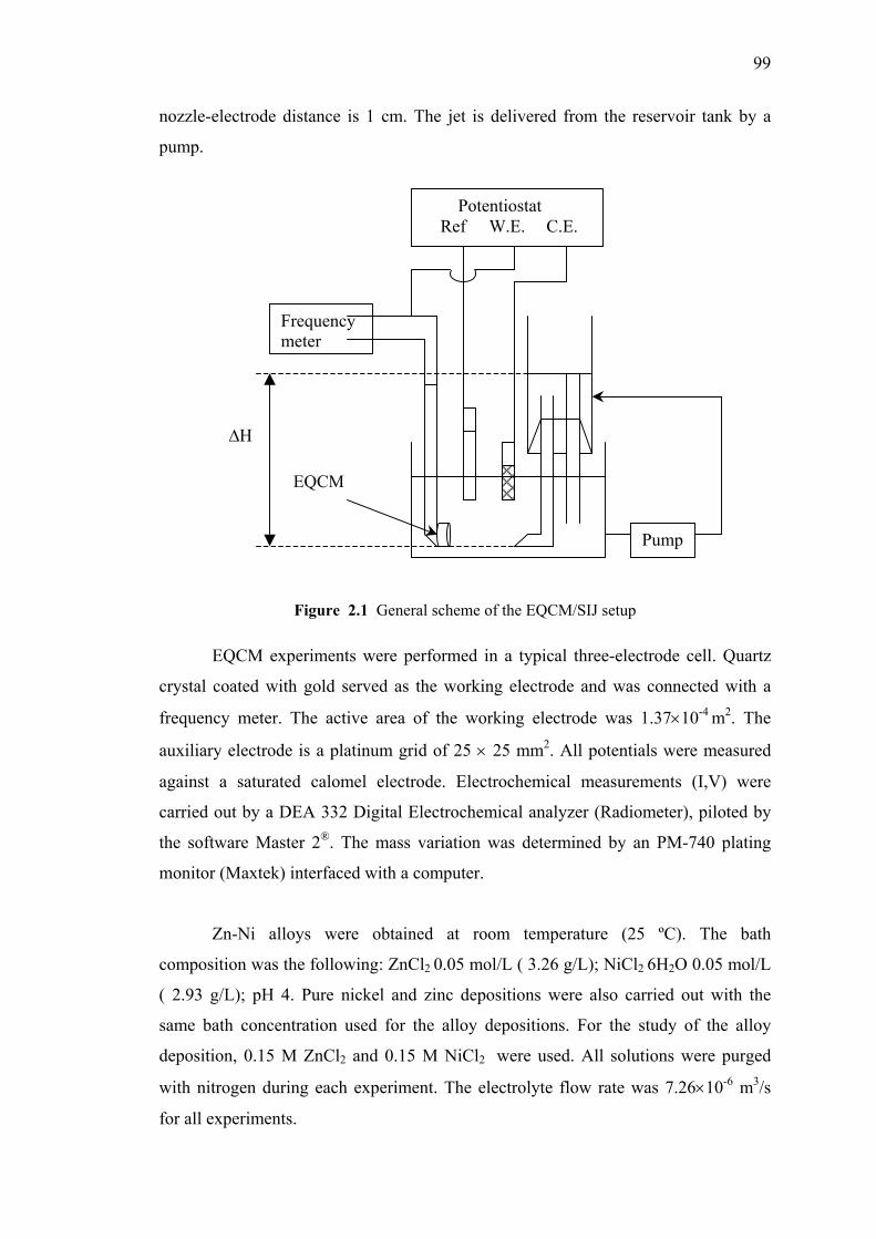
99

nozzle-electrode distance is 1 cm. The jet is delivered from the reservoir tank by a

pump.

Figure 2.1 General scheme of the EQCM/SIJ setup

EQCM experiments were performed in a typical three-electrode cell. Quartz

crystal coated with gold served as the working electrode and was connected with a

frequency meter. The active area of the working electrode was 1.37×10-4 m2. The

auxiliary electrode is a platinum grid of 25 × 25 mm2. All potentials were measured

against a saturated calomel electrode. Electrochemical measurements (I,V) were

carried out by a DEA 332 Digital Electrochemical analyzer (Radiometer), piloted by

the software Master 2®. The mass variation was determined by an PM-740 plating

monitor (Maxtek) interfaced with a computer.

Zn-Ni alloys were obtained at room temperature (25 ºC). The bath

composition was the following: ZnCl2 0.05 mol/L ( 3.26 g/L); NiCl2 6H2O 0.05 mol/L

( 2.93 g/L); pH 4. Pure nickel and zinc depositions were also carried out with the

same bath concentration used for the alloy depositions. For the study of the alloy

deposition, 0.15 M ZnCl2 and 0.15 M NiCl2 were used. All solutions were purged

with nitrogen during each experiment. The electrolyte flow rate was 7.26×10-6 m3/s

for all experiments.

Frequency meter

∆H

EQCM

Potentiostat Ref W.E. C.E.

Pump

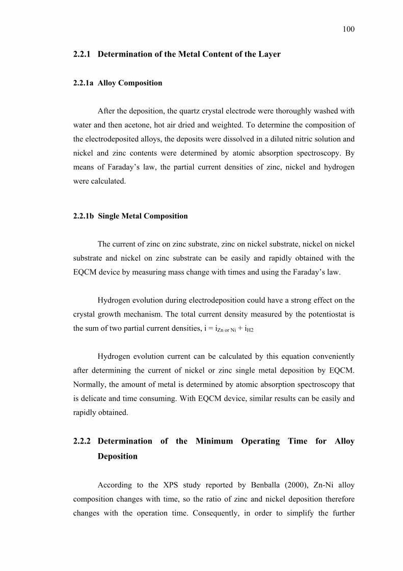
100

2.2.1 Determination of the Metal Content of the Layer

2.2.1a Alloy Composition

After the deposition, the quartz crystal electrode were thoroughly washed with

water and then acetone, hot air dried and weighted. To determine the composition of

the electrodeposited alloys, the deposits were dissolved in a diluted nitric solution and

nickel and zinc contents were determined by atomic absorption spectroscopy. By

means of Faraday’s law, the partial current densities of zinc, nickel and hydrogen

were calculated.

2.2.1b Single Metal Composition

The current of zinc on zinc substrate, zinc on nickel substrate, nickel on nickel

substrate and nickel on zinc substrate can be easily and rapidly obtained with the

EQCM device by measuring mass change with times and using the Faraday’s law.

Hydrogen evolution during electrodeposition could have a strong effect on the

crystal growth mechanism. The total current density measured by the potentiostat is

the sum of two partial current densities, i = iZn or Ni + iH2

Hydrogen evolution current can be calculated by this equation conveniently

after determining the current of nickel or zinc single metal deposition by EQCM.

Normally, the amount of metal is determined by atomic absorption spectroscopy that

is delicate and time consuming. With EQCM device, similar results can be easily and

rapidly obtained.

2.2.2 Determination of the Minimum Operating Time for Alloy

Deposition

According to the XPS study reported by Benballa (2000), Zn-Ni alloy

composition changes with time, so the ratio of zinc and nickel deposition therefore

changes with the operation time. Consequently, in order to simplify the further

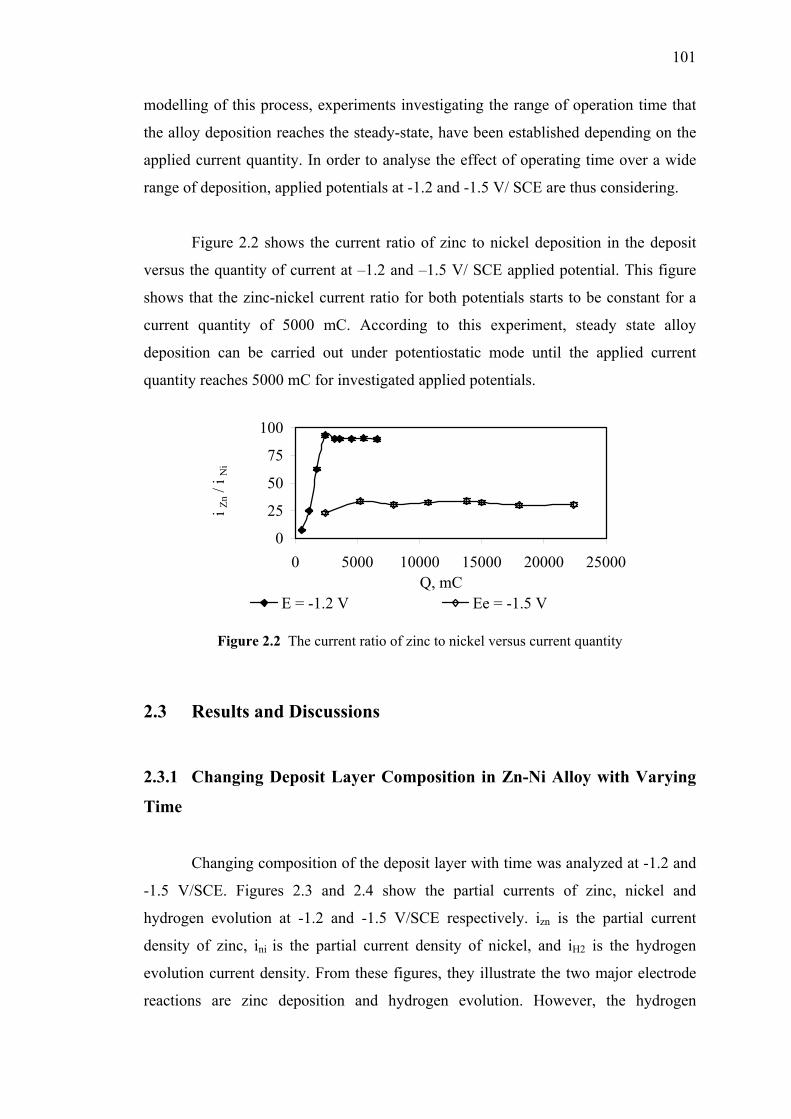
101

modelling of this process, experiments investigating the range of operation time that

the alloy deposition reaches the steady-state, have been established depending on the

applied current quantity. In order to analyse the effect of operating time over a wide

range of deposition, applied potentials at -1.2 and -1.5 V/ SCE are thus considering.

Figure 2.2 shows the current ratio of zinc to nickel deposition in the deposit

versus the quantity of current at –1.2 and –1.5 V/ SCE applied potential. This figure

shows that the zinc-nickel current ratio for both potentials starts to be constant for a

current quantity of 5000 mC. According to this experiment, steady state alloy

deposition can be carried out under potentiostatic mode until the applied current

quantity reaches 5000 mC for investigated applied potentials.

0

25

50

75

100

0 5000 10000 15000 20000 25000Q, mC

i Zn /

i N

i

E = -1.2 V Ee = -1.5 V Figure 2.2 The current ratio of zinc to nickel versus current quantity


2.3.1 Changing Deposit Layer Composition in Zn-Ni Alloy with Varying

Time

Changing composition of the deposit layer with time was analyzed at -1.2 and

-1.5 V/SCE. Figures 2.3 and 2.4 show the partial currents of zinc, nickel and

hydrogen evolution at -1.2 and -1.5 V/SCE respectively. izn is the partial current

density of zinc, ini is the partial current density of nickel, and iH2 is the hydrogen

evolution current density. From these figures, they illustrate the two major electrode

reactions are zinc deposition and hydrogen evolution. However, the hydrogen

102

evolution decays quickly from the initial stages of deposition. The nickel content in

the alloy decreases sharply and is being steady at 800 and 400 seconds, by applying

potential -1.2 and -1.5 V / SCE respectively.

2.3.1a Applied Potential at -1.2 V/SCE

With considering time ranging from 200 to 800 seconds, corresponding to the

initial stages of alloy deposition, nickel and hydrogen evolution contents are reduced,

while the current efficiency, zinc content and the ratio of Zn/Ni content are increased.

0

20

40

60

80

100

0 200 400 600 800 1000 1200 1400time, s

i Zn, i

H2,

i Zn/i N

i , A

/m2

00.10.20.30.40.50.60.7

iNi,

A/m

2

Figure 2.3 Nickel, zinc and hydrogen currents evolution versus the deposition time

Eapp = -1.2 V/ SCE. ZnCl2 0.05 mol/L, NiCl2 6H2O 0.05 mol/L and pH of 4

These results are similar to those of Lin and Selman, 1993 and Benballa et.

al., 2000 which observed high nickel and hydrogen evolution in the initial stages of

alloy deposition. Nickel will firstly deposit on substrate and act as catalyst for

hydrogen co-deposition, resulting in the very low cathodic current efficiency and zinc

content on the substrate. Afterwards, Zinc, being less catalytic than nickel, will

increasingly act as catalyst while nickel deposition and hydrogen evolution is

gradually reduced. Increasing both current efficiency and the surface coverage by zinc

deposition reduces the nickel content of the alloy. After the time 800 seconds, the

content of zinc, nickel, and hydrogen evolution are constant, and leads to a constant of

Zn/Ni current ratio and to a steady state deposition.

iZn iNi * iH2 x iZn/ iNi

103

The change of alloy composition observed with time relates to substrate effect.

Nickel deposits firstly on the gold electrode due to the less surface free energy

distribution. Zinc deposition on the preceding nickel substrate is the next step. Zinc is

more induced by the preceding nickel substrate than the gold electrode according to

the less surface free energy distribution taken by nickel 49.

According to this experiment, normal deposition mechanism was found at

initial operating time, as indicated in the literature, less than 50 seconds for

ammonium chloride bath43. It can be explained by the substrate effect. In Benbella ’s

works43, the XPS analysis (surface analysis) was applied for a real time indicator.

However, the cumulative indicator was used to analyze all the deposit composition

content in this experiment. As a result, there is more time taken for reaching a steady

state.

2.3.1b Applied Potential at -1.5 V/SCE

The mechanism of Zn-Ni alloy deposition can be explained as the applied

potential at -1.2 V/ SCE, changing the nature of electrode surface with time.

At this potential, the reduction rates of zinc and nickel are high compared to -

1.2 V/SCE. Zinc is able to deposit on the preceding nickel nuclei more rapidly. The

substrate layer grows faster because both intensities are bigger leading to blocking

and to decreasing of nickel content. Because of the high reduction of zinc at this

potential, the total current reaches the steady state at 400 seconds, while 800 seconds

are necessary for applied potential at-1.2 V/SCE.

These results indicate that the change of the electrode nature from gold

substrate to zinc-nickel substrate with time, due to the alloy deposition, affects the

total current relating to zinc and nickel contents on the electrode surface.

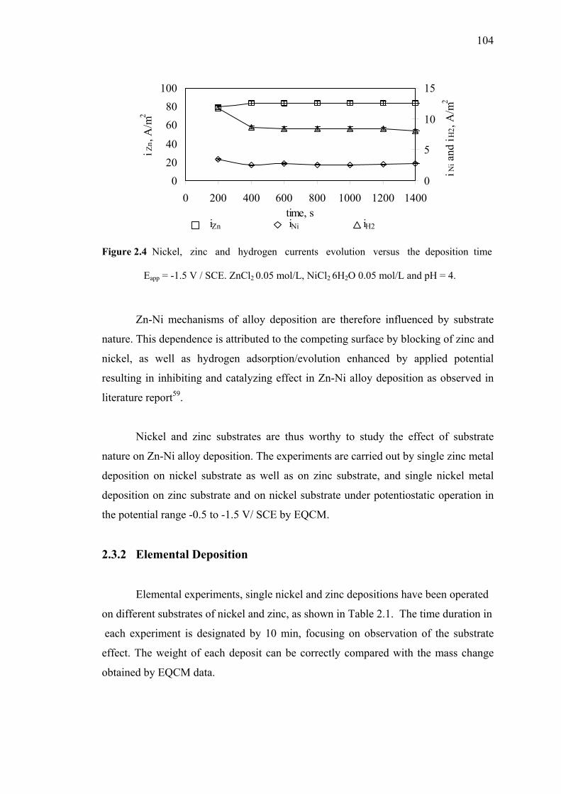
104

02040

6080

100

0 200 400 600 800 1000 1200 1400time, s

i Zn,

A/m

2

0

5

10

15

i Ni a

nd i H

2, A

/m2

iZn iNi iH2

Figure 2.4 Nickel, zinc and hydrogen currents evolution versus the deposition time

Eapp = -1.5 V / SCE. ZnCl2 0.05 mol/L, NiCl2 6H2O 0.05 mol/L and pH = 4.

Zn-Ni mechanisms of alloy deposition are therefore influenced by substrate

nature. This dependence is attributed to the competing surface by blocking of zinc and

nickel, as well as hydrogen adsorption/evolution enhanced by applied potential

resulting in inhibiting and catalyzing effect in Zn-Ni alloy deposition as observed in

literature report59.

Nickel and zinc substrates are thus worthy to study the effect of substrate

nature on Zn-Ni alloy deposition. The experiments are carried out by single zinc metal

deposition on nickel substrate as well as on zinc substrate, and single nickel metal

deposition on zinc substrate and on nickel substrate under potentiostatic operation in

the potential range -0.5 to -1.5 V/ SCE by EQCM.

2.3.2 Elemental Deposition

Elemental experiments, single nickel and zinc depositions have been operated

on different substrates of nickel and zinc, as shown in Table 2.1. The time duration in

each experiment is designated by 10 min, focusing on observation of the substrate

effect. The weight of each deposit can be correctly compared with the mass change

obtained by EQCM data.

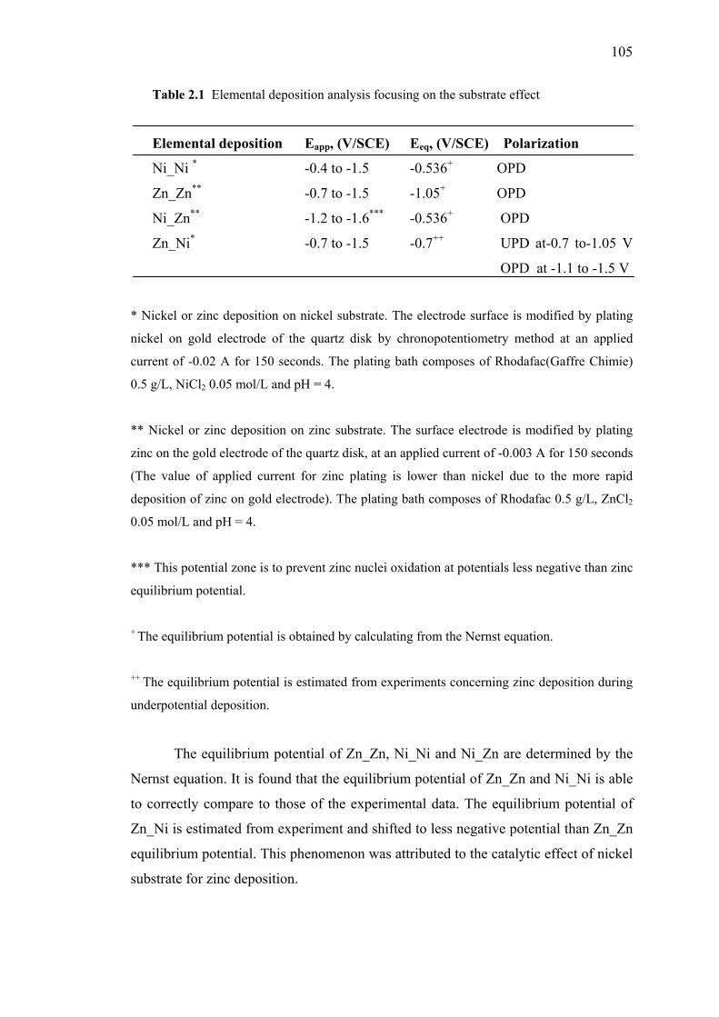
105

Table 2.1 Elemental deposition analysis focusing on the substrate effect

Elemental deposition Eapp, (V/SCE) Eeq, (V/SCE) Polarization

Ni_Ni * -0.4 to -1.5 -0.536+ OPD

Zn_Zn** -0.7 to -1.5 -1.05+ OPD

Ni_Zn** -1.2 to -1.6*** -0.536+ OPD

Zn_Ni* -0.7 to -1.5 -0.7++ UPD at-0.7 to-1.05 V

OPD at -1.1 to -1.5 V

* Nickel or zinc deposition on nickel substrate. The electrode surface is modified by plating

nickel on gold electrode of the quartz disk by chronopotentiometry method at an applied

current of -0.02 A for 150 seconds. The plating bath composes of Rhodafac(Gaffre Chimie)

0.5 g/L, NiCl2 0.05 mol/L and pH = 4.

** Nickel or zinc deposition on zinc substrate. The surface electrode is modified by plating

zinc on the gold electrode of the quartz disk, at an applied current of -0.003 A for 150 seconds

(The value of applied current for zinc plating is lower than nickel due to the more rapid

deposition of zinc on gold electrode). The plating bath composes of Rhodafac 0.5 g/L, ZnCl2

0.05 mol/L and pH = 4.

*** This potential zone is to prevent zinc nuclei oxidation at potentials less negative than zinc

equilibrium potential.

+ The equilibrium potential is obtained by calculating from the Nernst equation.

++ The equilibrium potential is estimated from experiments concerning zinc deposition during

underpotential deposition.

The equilibrium potential of Zn_Zn, Ni_Ni and Ni_Zn are determined by the

Nernst equation. It is found that the equilibrium potential of Zn_Zn and Ni_Ni is able

to correctly compare to those of the experimental data. The equilibrium potential of

Zn_Ni is estimated from experiment and shifted to less negative potential than Zn_Zn

equilibrium potential. This phenomenon was attributed to the catalytic effect of nickel

substrate for zinc deposition.

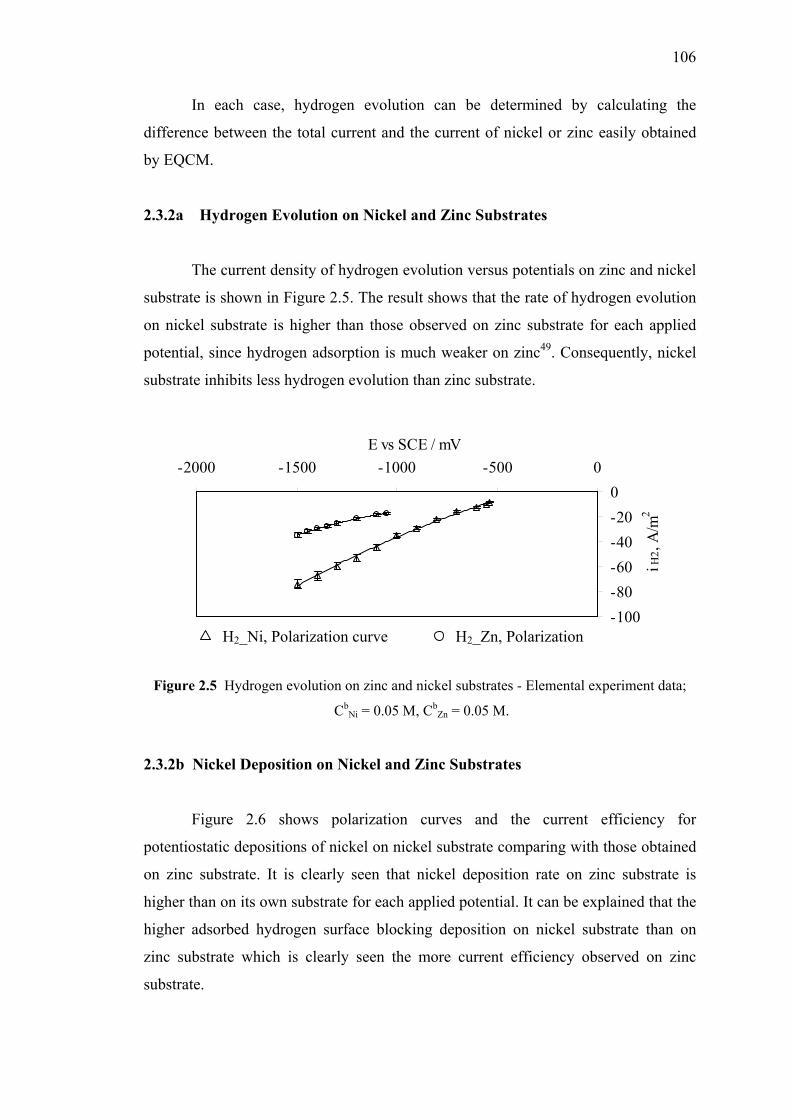
106

In each case, hydrogen evolution can be determined by calculating the

difference between the total current and the current of nickel or zinc easily obtained

by EQCM.

2.3.2a Hydrogen Evolution on Nickel and Zinc Substrates

The current density of hydrogen evolution versus potentials on zinc and nickel

substrate is shown in Figure 2.5. The result shows that the rate of hydrogen evolution

on nickel substrate is higher than those observed on zinc substrate for each applied

potential, since hydrogen adsorption is much weaker on zinc49. Consequently, nickel

substrate inhibits less hydrogen evolution than zinc substrate.

-100-80-60-40-200

-2000 -1500 -1000 -500 0E vs SCE / mV

i H2,

A/m

2

Figure 2.5 Hydrogen evolution on zinc and nickel substrates - Elemental experiment data;

CbNi = 0.05 M, Cb

Zn = 0.05 M.

2.3.2b Nickel Deposition on Nickel and Zinc Substrates

Figure 2.6 shows polarization curves and the current efficiency for

potentiostatic depositions of nickel on nickel substrate comparing with those obtained

on zinc substrate. It is clearly seen that nickel deposition rate on zinc substrate is

higher than on its own substrate for each applied potential. It can be explained that the

higher adsorbed hydrogen surface blocking deposition on nickel substrate than on

zinc substrate which is clearly seen the more current efficiency observed on zinc

substrate.

H2_Ni, Polarization curve H2_Zn, Polarization

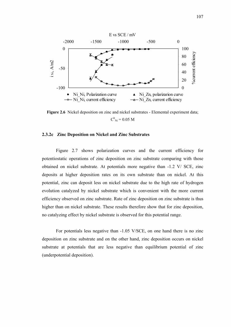
107

-100

-50

0-2000 -1500 -1000 -500 0

E vs SCE / mV

i Ni,

A/m

2

0

20

40

60

80

100

%cu

rrent

effi

cienc

y

Ni_Ni, Polarization curve Ni_Zn, polarizarion curveNi_Ni, current efficiency Ni_Zn, current efficiency

Figure 2.6 Nickel deposition on zinc and nickel substrates - Elemental experiment data;

CbNi = 0.05 M

2.3.2c Zinc Deposition on Nickel and Zinc Substrates

Figure 2.7 shows polarization curves and the current efficiency for

potentiostatic operations of zinc deposition on zinc substrate comparing with those

obtained on nickel substrate. At potentials more negative than -1.2 V/ SCE, zinc

deposits at higher deposition rates on its own substrate than on nickel. At this

potential, zinc can deposit less on nickel substrate due to the high rate of hydrogen

evolution catalyzed by nickel substrate which is convenient with the more current

efficiency observed on zinc substrate. Rate of zinc deposition on zinc substrate is thus

higher than on nickel substrate. These results therefore show that for zinc deposition,

no catalyzing effect by nickel substrate is observed for this potential range.

For potentials less negative than -1.05 V/SCE, on one hand there is no zinc

deposition on zinc substrate and on the other hand, zinc deposition occurs on nickel

substrate at potentials that are less negative than equilibrium potential of zinc

(underpotential deposition).

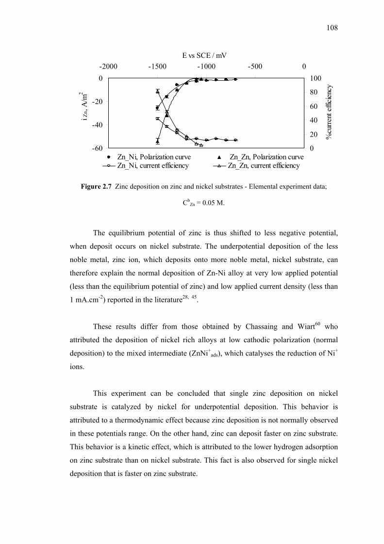
108

-60

-40

-20

0-2000 -1500 -1000 -500 0

E vs SCE / mV

i Zn,

A/m

2

0

20

40

60

80

100

%cu

rrent

effi

cienc

y

Zn_Ni, Polarization curve Zn_Zn, Polarization curveZn_Ni, current efficiency Zn_Zn, current efficiency

Figure 2.7 Zinc deposition on zinc and nickel substrates - Elemental experiment data;

CbZn = 0.05 M.

The equilibrium potential of zinc is thus shifted to less negative potential,

when deposit occurs on nickel substrate. The underpotential deposition of the less

noble metal, zinc ion, which deposits onto more noble metal, nickel substrate, can

therefore explain the normal deposition of Zn-Ni alloy at very low applied potential

(less than the equilibrium potential of zinc) and low applied current density (less than

1 mA.cm-2) reported in the literature28, 45.

These results differ from those obtained by Chassaing and Wiart60 who

attributed the deposition of nickel rich alloys at low cathodic polarization (normal

deposition) to the mixed intermediate (ZnNi+ads), which catalyses the reduction of Ni+

ions.

This experiment can be concluded that single zinc deposition on nickel

substrate is catalyzed by nickel for underpotential deposition. This behavior is

attributed to a thermodynamic effect because zinc deposition is not normally observed

in these potentials range. On the other hand, zinc can deposit faster on zinc substrate.

This behavior is a kinetic effect, which is attributed to the lower hydrogen adsorption

on zinc substrate than on nickel substrate. This fact is also observed for single nickel

deposition that is faster on zinc substrate.

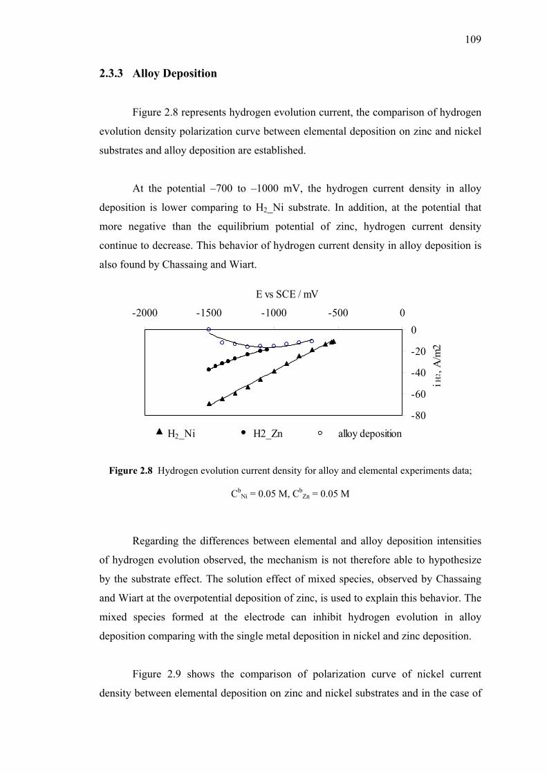
109

2.3.3 Alloy Deposition

Figure 2.8 represents hydrogen evolution current, the comparison of hydrogen

evolution density polarization curve between elemental deposition on zinc and nickel

substrates and alloy deposition are established.

At the potential –700 to –1000 mV, the hydrogen current density in alloy

deposition is lower comparing to H2_Ni substrate. In addition, at the potential that

more negative than the equilibrium potential of zinc, hydrogen current density

continue to decrease. This behavior of hydrogen current density in alloy deposition is

also found by Chassaing and Wiart.

-80

-60

-40

-20

0-2000 -1500 -1000 -500 0

E vs SCE / mV

i H2 ,

A/m

2 H2_Ni H2_Zn alloy deposition

Figure 2.8 Hydrogen evolution current density for alloy and elemental experiments data;

CbNi = 0.05 M, Cb

Zn = 0.05 M

Regarding the differences between elemental and alloy deposition intensities

of hydrogen evolution observed, the mechanism is not therefore able to hypothesize

by the substrate effect. The solution effect of mixed species, observed by Chassaing

and Wiart at the overpotential deposition of zinc, is used to explain this behavior. The

mixed species formed at the electrode can inhibit hydrogen evolution in alloy

deposition comparing with the single metal deposition in nickel and zinc deposition.

Figure 2.9 shows the comparison of polarization curve of nickel current

density between elemental deposition on zinc and nickel substrates and in the case of

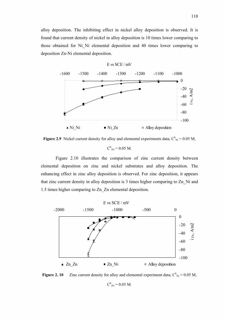
110

alloy deposition. The inhibiting effect in nickel alloy deposition is observed. It is

found that current density of nickel in alloy deposition is 10 times lower comparing to

those obtained for Ni_Ni elemental deposition and 40 times lower comparing to

deposition Zn-Ni elemental deposition.

-100

-80

-60

-40

-20

0-1600 -1500 -1400 -1300 -1200 -1100 -1000

E vs SCE / mV

i Ni,

A/m

2

Ni_Ni Ni_Zn Alloy deposition

Figure 2.9 Nickel current density for alloy and elemental experiments data; CbNi = 0.05 M,

CbZn = 0.05 M.

Figure 2.10 illustrates the comparison of zinc current density between

elemental deposition on zinc and nickel substrates and alloy deposition. The

enhancing effect in zinc alloy deposition is observed. For zinc deposition, it appears

that zinc current density in alloy deposition is 3 times higher comparing to Zn_Ni and

1.5 times higher comparing to Zn_Zn elemental deposition.

-100

-80

-60

-40

-20

0-2000 -1500 -1000 -500 0

E vs SCE / mV

i Zn,

A/m

2

Zn_Zn Zn_Ni Alloy deposition

Figure 2. 10 Zinc current density for alloy and elemental experiment data; CbNi = 0.05 M,

CbZn = 0.05 M.

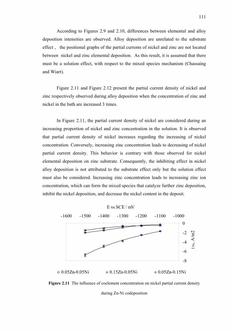
111

According to Figures 2.9 and 2.10, differences between elemental and alloy

deposition intensities are observed. Alloy deposition are unrelated to the substrate

effect , the positional graphs of the partial currents of nickel and zinc are not located

between nickel and zinc elemental deposition. As this result, it is assumed that there

must be a solution effect, with respect to the mixed species mechanism (Chassaing

and Wiart).

Figure 2.11 and Figure 2.12 present the partial current density of nickel and

zinc respectively observed during alloy deposition when the concentration of zinc and

nickel in the bath are increased 3 times.

In Figure 2.11, the partial current density of nickel are considered during an

increasing proportion of nickel and zinc concentration in the solution. It is observed

that partial current density of nickel increases regarding the increasing of nickel

concentration. Conversely, increasing zinc concentration leads to decreasing of nickel

partial current density. This behavior is contrary with those observed for nickel

elemental deposition on zinc substrate. Consequently, the inhibiting effect in nickel

alloy deposition is not attributed to the substrate effect only but the solution effect

must also be considered. Increasing zinc concentration leads to increasing zinc ion

concentration, which can form the mixed species that catalyze further zinc deposition,

inhibit the nickel deposition, and decrease the nickel content in the deposit.

-8

-6

-4

-2

0-1600 -1500 -1400 -1300 -1200 -1100 -1000

E vs SCE / mV

i Ni,

A/m

2

0.05Zn-0.05Ni 0.15Zn-0.05Ni 0.05Zn-0.15Ni

Figure 2.11 The influence of coelement concentration on nickel partial current density

during Zn-Ni codeposition

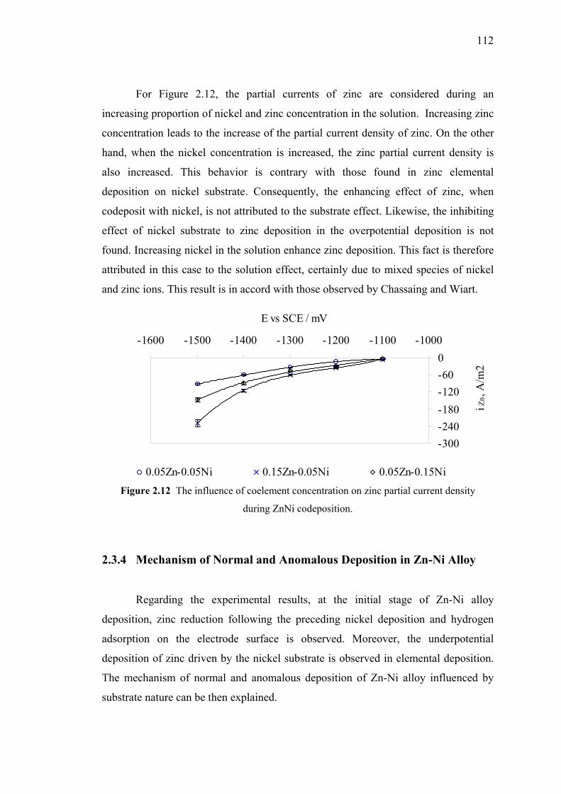
112

For Figure 2.12, the partial currents of zinc are considered during an

increasing proportion of nickel and zinc concentration in the solution. Increasing zinc

concentration leads to the increase of the partial current density of zinc. On the other

hand, when the nickel concentration is increased, the zinc partial current density is

also increased. This behavior is contrary with those found in zinc elemental

deposition on nickel substrate. Consequently, the enhancing effect of zinc, when

codeposit with nickel, is not attributed to the substrate effect. Likewise, the inhibiting

effect of nickel substrate to zinc deposition in the overpotential deposition is not

found. Increasing nickel in the solution enhance zinc deposition. This fact is therefore

attributed in this case to the solution effect, certainly due to mixed species of nickel

and zinc ions. This result is in accord with those observed by Chassaing and Wiart.

-300-240-180-120-600

-1600 -1500 -1400 -1300 -1200 -1100 -1000

E vs SCE / mV

i Zn,

A/m

20.05Zn-0.05Ni 0.15Zn-0.05Ni 0.05Zn-0.15Ni

Figure 2.12 The influence of coelement concentration on zinc partial current density

during ZnNi codeposition.

2.3.4 Mechanism of Normal and Anomalous Deposition in Zn-Ni Alloy

Regarding the experimental results, at the initial stage of Zn-Ni alloy

deposition, zinc reduction following the preceding nickel deposition and hydrogen

adsorption on the electrode surface is observed. Moreover, the underpotential

deposition of zinc driven by the nickel substrate is observed in elemental deposition.

The mechanism of normal and anomalous deposition of Zn-Ni alloy influenced by

substrate nature can be then explained.

113

The normal deposition can be explained by the following mechanism. At the

initial stage, a high deposition of nickel happens because nickel more noble properties

and then catalyses hydrogen adsorption, leading to high nickel and hydrogen

evolution observed in the beginning of Zn-Ni alloy deposit. In the later stage, the

deposited nickel at the initial stage induces zinc reduction in an underpotential

deposition mode. As a result, rich nickel content and low zinc content always occur in

the low potential operation. In addition, Zinc reduction is still not high in this normal

deposition.

However, when the applied potential is higher than the equilibrium potential

of zinc, high zinc deposition rates occur, resulting in anomalous deposition. This

circumstance could happen after hydrogen adsorption and nickel deposition in the

early stage of the deposition process. Nickel substrate does not catalyze zinc

deposition at the overpotential of zinc, in the elemental deposition analysis. This

means the enhancement of zinc deposition can not be explained by the substrate

effect. Anomalous deposition therefore is not the substrate relate. According to the

alloy deposition experiments, the anomalous deposition is explained by the solution

effect. It’s possible that zinc codeposits with nickel to form a mixed species of nickel

and zinc ion leading to an enhancement of zinc deposition. The anomalous deposition

is thus hypothesized by the mixed species effect in the high polarization.

2.4 Conclusion

Zn-Ni alloy potentiostatic electrodepositions in the range -0.7 to -1.5 V / SCE

by EQCM and the study of Zn-Ni alloy composition changing with time have been

analyzed. The mechanism of Zn-Ni alloy deposition depending on the applied

potential and the scale time considered can be hypothesized.

(i) Normal deposition mechanism in Zn-Ni alloy for low polarization is

due to the underpotential deposition of zinc driven by the preceding

nickel nuclei depositing at the initial deposition stage. (substrate effect)

114

(ii) The enhancing effect of zinc and the inhibiting effect of nickel are

found in alloy deposition. It leads to the anomalous deposition which

attributes to the solution effect at the high polarization, due to the

mixed species at the steady state.

(iii) For time less than 800 seconds, the time deposition has an effect on the

composition of the deposit. This effect was attributed to a substrate

related.

115

Chapter 3

Mathematical Modelling of Zn-Ni Alloy Deposition

According to the experimental results in chapter 2, the substrate has an effect

on the mechanism of Zn-Ni deposition, especially at the initial stage deposition and the

UPD of zinc on nickel substrate. On the other hand, the solution has an effect on the

mechanism of Zn-Ni deposition at the overpotential deposition of zinc. The solution

effect is due to the mixed species observed by Wiart and Zech in the literature reports.

This chapter is composed of models explaining Zn-Ni mechanism in terms of substrate

and solution effect.

3.1 Substrate Effect Model

3.1.1 Introduction

In chapter 2, the electrodeposition of Zn-Ni alloy is investigated. It is

suggested that initial nuclei of nickel adsorbed on the electrode surface act as a

substrate to catalyse zinc deposition, resulting in inhibiting nickel deposition. It is also

shown that pure zinc cannot be electrodeposited from aqueous electrolytes at the

UPD, but can be codeposited with nickel. These phenomena can be explained that

nickel nuclei deposited firstly with hydrogen atom as an adsorbed species to catalyse

zinc deposition. At more negative potential than equilibrium potential of zinc, zinc

deposition rate is high enough, and inhibits nickel deposition resulting in “Anomalous

deposition”. The purpose of this research is to verify the experimental result of Zn-Ni

alloy codeposition taking into account the substrate effects, from chapter 1.

3.1.2 Model Assumption

In this chapter, a mathematical model describing the codeposition behaviour

of nickel and zinc, in a more quantitative way, is presented. According to the

experimental result of chapter 2, the adsorbed nuclei of nickel acting as a substrate to

catalyse zinc deposition is of great value to make a model, Zn-Ni alloy mechanism

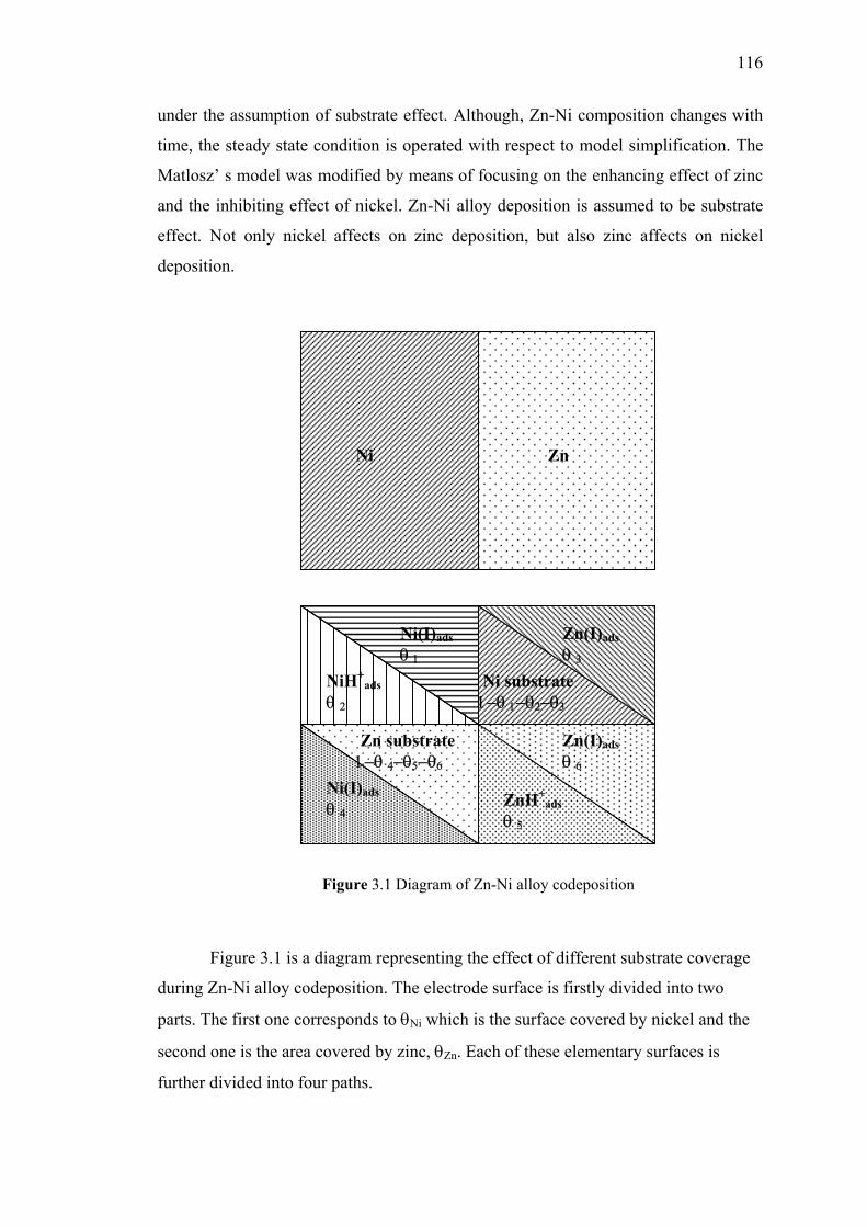
116

under the assumption of substrate effect. Although, Zn-Ni composition changes with

time, the steady state condition is operated with respect to model simplification. The

Matlosz’ s model was modified by means of focusing on the enhancing effect of zinc

and the inhibiting effect of nickel. Zn-Ni alloy deposition is assumed to be substrate

effect. Not only nickel affects on zinc deposition, but also zinc affects on nickel

deposition.

Figure 3.1 Diagram of Zn-Ni alloy codeposition

Figure 3.1 is a diagram representing the effect of different substrate coverage

during Zn-Ni alloy codeposition. The electrode surface is firstly divided into two

parts. The first one corresponds to θNi which is the surface covered by nickel and the

second one is the area covered by zinc, θZn. Each of these elementary surfaces is

further divided into four paths.

Ni(I)ads

θ 1

NiH+ads

θ 2

Ni substrate

1−θ 1−θ2−θ3

Zn(I)ads

θ 3

Zn(I)ads θ 6

Zn substrate 1−θ 4−θ5−θ6

ZnH+

ads

θ 5

Ni(I)ads

θ 4

Ni Zn

117

In case of nickel alloy deposition, θNiθ1 corresponds to the surface area of

nickel substrate covered by Ni(I)ads. θNiθ2 corresponds to the surface area of nickel

substrate covered by NiH+ads. θNiθ3 corresponds to the surface area of nickel substrate

covered by Zn(I)ads. The free surface area θNi(1-θ1-θ2-θ3) corresponds to the surface

area of nickel substrate path.

In case of zinc alloy deposition, θZnθ6 corresponds to the surface area of zinc

substrate covered by Zn(I)ads. θZnθ5 corresponds to the surface area of zinc substrate

covered by ZnH+ads. θZnθ4 corresponds to the surface area of zinc substrate covered by

Ni(I)ads. The free surface area θZn(1-θ4-θ5-θ6 ) corresponds to the surface area of zinc

substrate path.

3.1.3 Theoretical Model

3.1.3.1 General Mechanism of the Electrode Reaction

A reaction path has been developed by the basis of the substrate effect. The

present model is assumed that the deposition of each individual component follows a

two-step reaction as described by Matlosz. Nickel ion can deposit on its own substrate

and on zinc’s substrate according to reaction 1 and 2 respectively. Also, Zinc ion can

deposit on zinc’s substrate and on nickel’s substrate as seen in reaction 4 and 5. In

addition, the reactions of the hydrogenated blocking the adsorbent ZnH+ads and

NiH+ads , are supposed to be strongly bonded to the electrode surface and taken into

account as reaction 3 and 6 respectively.

Ni(II) will react to give NiH+ads and this adsorbed species will then react to

deposit Ni. Also, Zn (II) will react to give ZnH+ads and then this absorbed species

has to react to deposit Zn. Depending upon the substrate, the first step (adsorption)

could have a different kinetics.

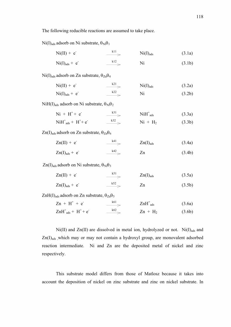
118

The following reducible reactions are assumed to take place.

Ni(I)ads adsorb on Ni substrate, θNiθ1

Ni(II) + e- k11 Ni(I)ads (3.1a)

Ni(I)ads + e- k12 Ni (3.1b)

Ni(I)ads adsorb on Zn substrate, θZnθ4


Ni(I)ads + e- k22 Ni (3.2b)

NiH(I)ads adsorb on Ni substrate, θNiθ2

Ni + H+ + e- k31 NiH+ads (3.3a)

NiH+ads + H++ e- k32 Ni + H2 (3.3b)

Zn(I)ads adsorb on Zn substrate, θZnθ6

Zn(II) + e- k41 Zn(I)ads (3.4a)

Zn(I)ads + e- k42 Zn (3.4b)

Zn(I)ads adsorb on Ni substrate, θNiθ3


Zn(I)ads + e- k52 Zn (3.5b)

ZnH(I)ads adsorb on Zn substrate, θZnθ5

Zn + H+ + e- k61 ZnH+ads (3.6a)

ZnH+ads + H+ + e- k62 Zn + H2 (3.6b)

Ni(II) and Zn(II) are dissolved in metal ion, hydrolyzed or not. Ni(I)ads and

Zn(I)ads ,which may or may not contain a hydroxyl group, are monovalent adsorbed

reaction intermediate. Ni and Zn are the deposited metal of nickel and zinc

respectively.

This substrate model differs from those of Matlosz because it takes into

account the deposition of nickel on zinc substrate and zinc on nickel substrate. In

119

addition, this model explains both the inhibition effect of nickel deposition and the

enhancing effect of zinc deposition, observed in Zn-Ni alloy codeposition.

3.1.3.2 Mass Transfer Effect

The model further assumes steady state conditions. Concentration variations

are restricted to a thin boundary layer near the electrode surface. Mass transport

across this layer is governed by diffusion. Migration effects are considered to be

negligible.

The steady state material balances within the diffusion layer for species Ni(II),

Zn(II) and H+, 0<x<d, can be written in order to investigate the concentration in the

diffusion layer.

(3.7)

(3.8)

(3.9)

(3.10)

Assuming a constant diffusion coefficient, D, the flux of each species i, in the

diffusion layer is Ni = -D dCi / dx. The assumed values of the diffusion coefficients

are 4×10-10 m2 s-1 for Ni(II), 5.09×10-10 m2 s-1 for Zn(II), and 9.3×10-9 m2 s-1 for

solvated protons, and 5.5×10-9 m2 s-1 for hydroxide ions59.

The intermediate species, Ni(I)ads, NiH+ads, Zn(I)ads and ZnH+

ads exist only at

the electrode surface so their concentration are equal to zero in the solution. At the

electrode surface (x = 0), the partial current densities are related to the species fluxes

by the following reaction:

+⋅−=

=+⋅∇=⋅∇=⋅∇

HOH

H

Zn(II)Ni(II)

CCwK0N0N0N

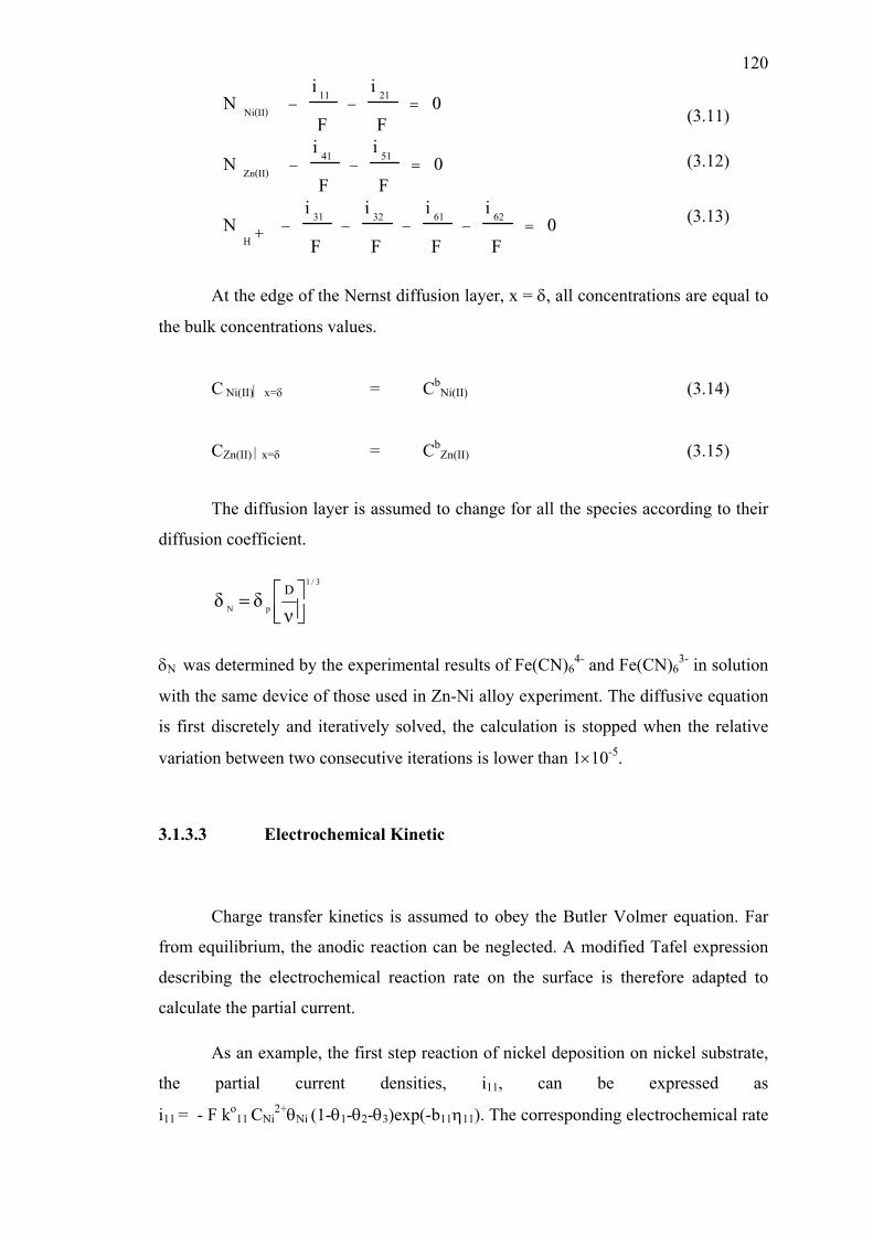
120

(3.11)

(3.12)

(3.13)

At the edge of the Nernst diffusion layer, x = δ, all concentrations are equal to

the bulk concentrations values.

C Ni(II) x=δ = CbNi(II) (3.14)

CZn(II) x=δ = Cb

Zn(II) (3.15)

The diffusion layer is assumed to change for all the species according to their

diffusion coefficient.

3/1

pND

=ν

δδ

δΝ was determined by the experimental results of Fe(CN)64- and Fe(CN)6

3- in solution

with the same device of those used in Zn-Ni alloy experiment. The diffusive equation

is first discretely and iteratively solved, the calculation is stopped when the relative

variation between two consecutive iterations is lower than 1×10-5.

3.1.3.3 Electrochemical Kinetic

Charge transfer kinetics is assumed to obey the Butler Volmer equation. Far

from equilibrium, the anodic reaction can be neglected. A modified Tafel expression

describing the electrochemical reaction rate on the surface is therefore adapted to

calculate the partial current.

As an example, the first step reaction of nickel deposition on nickel substrate,

the partial current densities, i11, can be expressed as

i11 = - F ko11 CNi

2+θNi (1-θ1-θ2-θ3)exp(-b11η11). The corresponding electrochemical rate

0F

iF

iF

iF

iN

0F

iF

iN

0F

iF

iN

62613231H

5141Zn(II)

2111Ni(II)

=−−−−+

=−−

=−−

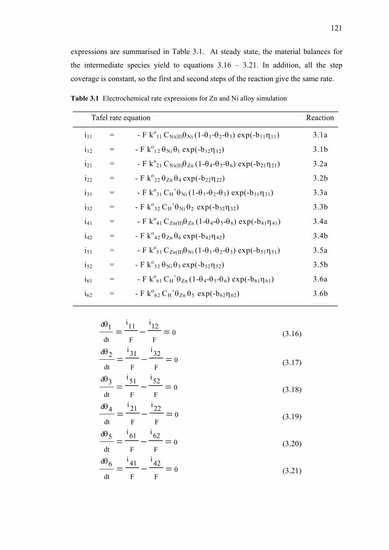
121

expressions are summarised in Table 3.1. At steady state, the material balances for

the intermediate species yield to equations 3.16 – 3.21. In addition, all the step

coverage is constant, so the first and second steps of the reaction give the same rate.

Table 3.1 Electrochemical rate expressions for Zn and Ni alloy simulation

Tafel rate equation Reaction

i11 = - F ko11 CNi(II)θNi (1-θ1-θ2-θ3) exp(-b11η11) 3.1a

i12 = - F kο12 θNi θ1 exp(-b12η12) 3.1b

i21 = - F ko21 CNi(II)θZn (1-θ4-θ5-θ6) exp(-b21η21) 3.2a

i22 = - F kο22 θZn θ4 exp(-b22η22) 3.2b

i31 = - F ko31 CH

+θNi (1-θ1-θ2-θ3) exp(-b31η31) 3.3a

i32 = - F kο32 CH

+θNi θ2 exp(-b32η32) 3.3b

i41 = - F ko41 CZn(II)θZn (1-θ4-θ5-θ6) exp(-b41η41) 3.4a

i42 = - F kο42 θZn θ6 exp(-b42η42) 3.4b

i51 = - F ko51 CZn(II)θNi (1-θ1-θ2-θ3) exp(-b51η51) 3.5a

i52 = - F kο52 θNi θ3 exp(-b52η52) 3.5b

i61 = - F ko61 CH

+θZn (1-θ4-θ5-θ6) exp(-b61η61) 3.6a

i62 = - F kο62 CH

+θZn θ5 exp(-b62η62) 3.6b

(3.16) (3.17) (3.18) (3.19) (3.20) (3.21)

0F42i

F41i

dt6d

0F62i

F61i

dt5d

0F22i

F21i

dt4d

0F52i

F51i

dt3d

0F32i

F31i

dt2d

0F12i

F11i

dt1d

=−=

=−=

=−=

=−=

=−=

=−=

θ

θ

θ

θ

θ

θ

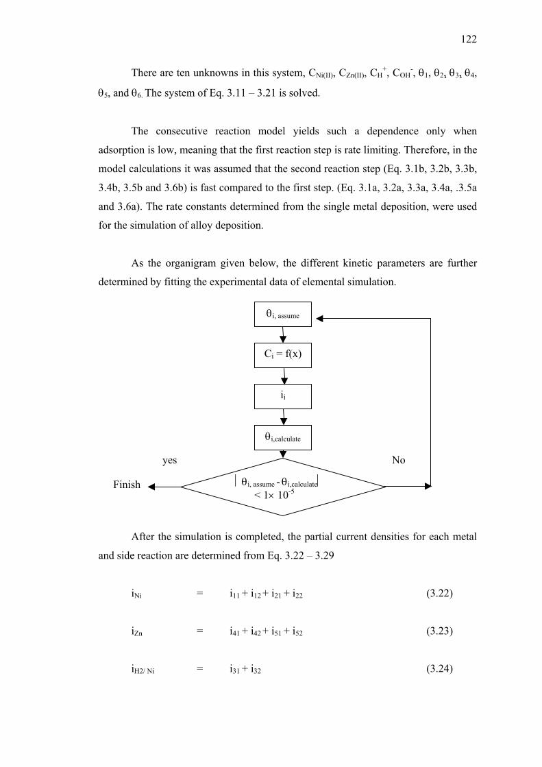
122

There are ten unknowns in this system, CNi(II), CZn(II), CH+, COH

-, θ1, θ2, θ3, θ4,

θ5, and θ6. The system of Eq. 3.11 – 3.21 is solved.

The consecutive reaction model yields such a dependence only when

adsorption is low, meaning that the first reaction step is rate limiting. Therefore, in the

model calculations it was assumed that the second reaction step (Eq. 3.1b, 3.2b, 3.3b,

3.4b, 3.5b and 3.6b) is fast compared to the first step. (Eq. 3.1a, 3.2a, 3.3a, 3.4a, .3.5a

and 3.6a). The rate constants determined from the single metal deposition, were used

for the simulation of alloy deposition.

As the organigram given below, the different kinetic parameters are further

determined by fitting the experimental data of elemental simulation.

After the simulation is completed, the partial current densities for each metal

and side reaction are determined from Eq. 3.22 – 3.29

iNi = i11 + i12 + i21 + i22 (3.22) iZn = i41 + i42 + i51 + i52 (3.23) iH2/ Ni

= i31 + i32 (3.24)

θi, assume

Ci = f(x)

ii

θi,calculate

yes No

Finish θi, assume - θi,calculate < 1× 10-5

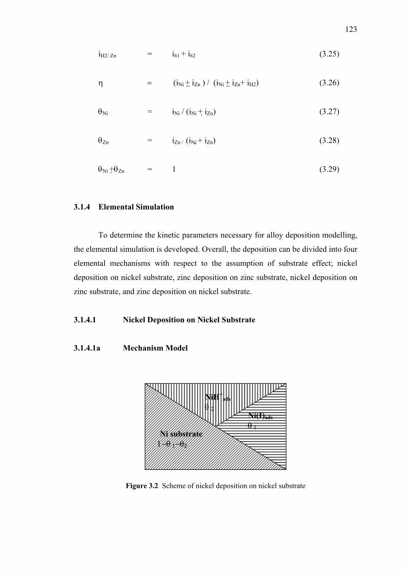
123

iH2/ Zn = i61 + i62 (3.25)

η = (iNi + iZn ) / (iNi + iZn+ iH2) (3.26) θNi = iNi / (iNi + iZn) (3.27) θZn = iZn / (iNi + iZn) (3.28) θNi + θZn = 1 (3.29)

3.1.4 Elemental Simulation

To determine the kinetic parameters necessary for alloy deposition modelling,

the elemental simulation is developed. Overall, the deposition can be divided into four

elemental mechanisms with respect to the assumption of substrate effect; nickel

deposition on nickel substrate, zinc deposition on zinc substrate, nickel deposition on

zinc substrate, and zinc deposition on nickel substrate.

3.1.4.1 Nickel Deposition on Nickel Substrate

3.1.4.1a Mechanism Model

Figure 3.2 Scheme of nickel deposition on nickel substrate

Ni(I)ads

θ 1

NiH+ads

θ 2

Ni substrate

1−θ 1−θ2

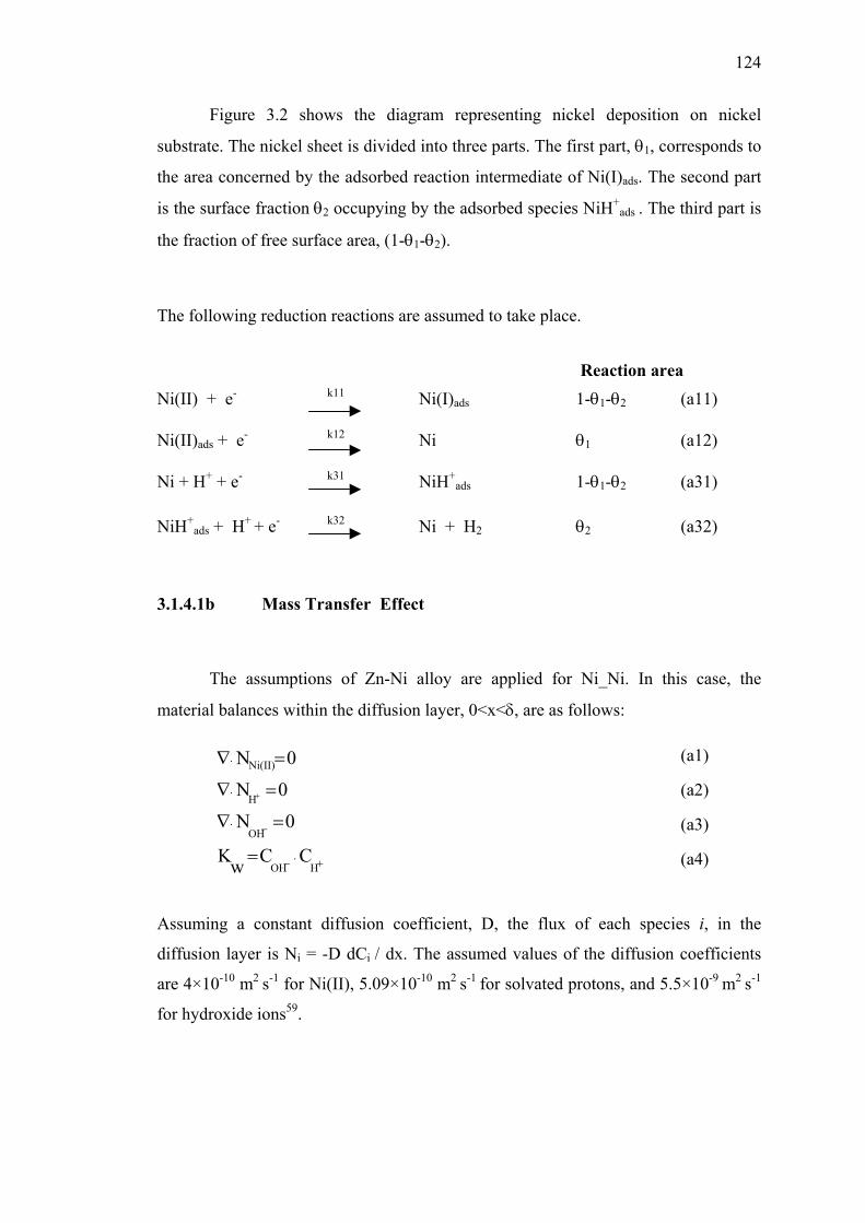
124

Figure 3.2 shows the diagram representing nickel deposition on nickel

substrate. The nickel sheet is divided into three parts. The first part, θ1, corresponds to

the area concerned by the adsorbed reaction intermediate of Ni(I)ads. The second part

is the surface fraction θ2 occupying by the adsorbed species NiH+ads . The third part is

the fraction of free surface area, (1-θ1-θ2).

The following reduction reactions are assumed to take place.

Reaction area Ni(II) + e- k11 Ni(I)ads 1-θ1-θ2 (a11) Ni(II)ads + e- k12 Ni θ1 (a12) Ni + H+ + e- k31 NiH+

ads 1-θ1-θ2 (a31) NiH+

ads + H+ + e- k32 Ni + H2 θ2 (a32)

3.1.4.1b Mass Transfer Effect

The assumptions of Zn-Ni alloy are applied for Ni_Ni. In this case, the

material balances within the diffusion layer, 0<x<δ, are as follows:

(a1)

(a2)

(a3)

(a4)



are 4×10-10 m2 s-1 for Ni(II), 5.09×10-10 m2 s-1 for solvated protons, and 5.5×10-9 m2 s-1

for hydroxide ions59.

+⋅−

−⋅

⋅

⋅

=

=∇

=∇

=∇

+

HOH

OH

H

Ni(II)

CCwK

0N

0N

0N

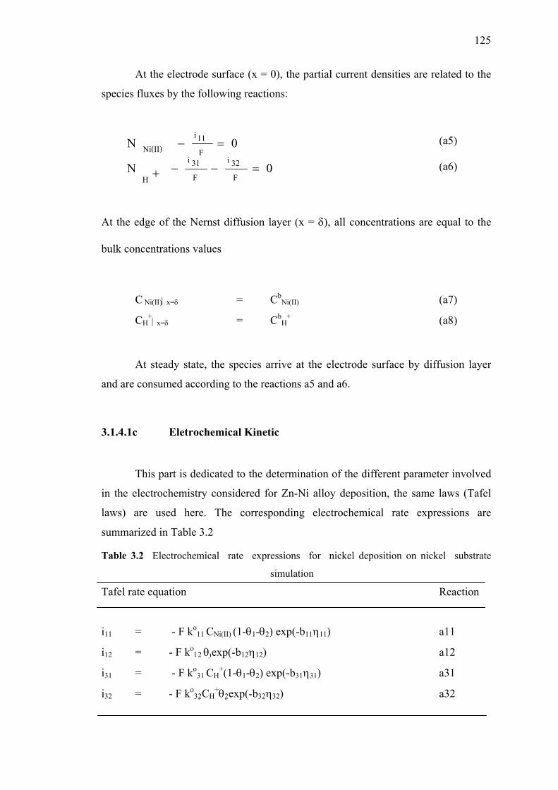
125

At the electrode surface (x = 0), the partial current densities are related to the

species fluxes by the following reactions:

(a5)

(a6)

At the edge of the Nernst diffusion layer (x = δ), all concentrations are equal to the

bulk concentrations values

C Ni(II)x=δ = CbNi(II) (a7)

CH+

x=δ = CbH

+ (a8)

At steady state, the species arrive at the electrode surface by diffusion layer

and are consumed according to the reactions a5 and a6.

3.1.4.1c Eletrochemical Kinetic

This part is dedicated to the determination of the different parameter involved

in the electrochemistry considered for Zn-Ni alloy deposition, the same laws (Tafel

laws) are used here. The corresponding electrochemical rate expressions are

summarized in Table 3.2

Table 3.2 Electrochemical rate expressions for nickel deposition on nickel substrate

simulation


i11 = - F ko11 CNi(II) (1-θ1-θ2) exp(-b11η11) a11

i12 = - F kο12 θexp(-b12η12) a12

i31 = - F ko31 CH

+(1-θ1-θ2) exp(-b31η31) a31

i32 = - F kο32CH

+θ2 exp(-b32η32) a32

0N0N

F32i

F31i

H

F11i

Ni(II)=−−+

=−

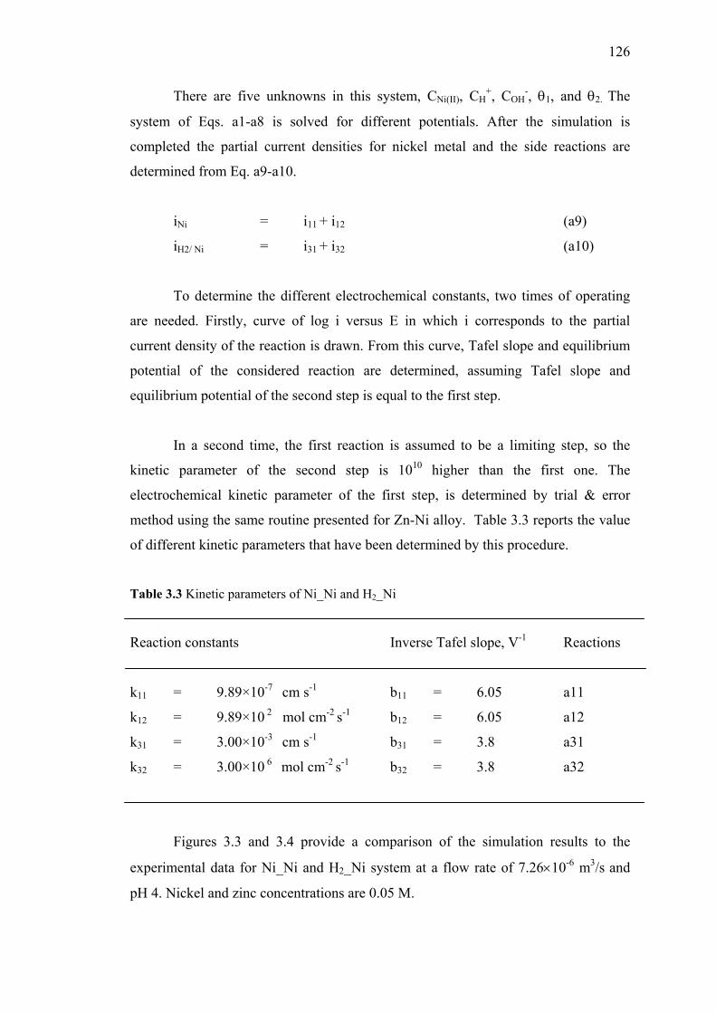
126

There are five unknowns in this system, CNi(II), CH+, COH

-, θ1, and θ2. The

system of Eqs. a1-a8 is solved for different potentials. After the simulation is

completed the partial current densities for nickel metal and the side reactions are

determined from Eq. a9-a10.

iNi = i11 + i12 (a9)

iH2/ Ni = i31 + i32 (a10)

To determine the different electrochemical constants, two times of operating

are needed. Firstly, curve of log i versus E in which i corresponds to the partial

current density of the reaction is drawn. From this curve, Tafel slope and equilibrium

potential of the considered reaction are determined, assuming Tafel slope and

equilibrium potential of the second step is equal to the first step.

In a second time, the first reaction is assumed to be a limiting step, so the

kinetic parameter of the second step is 1010 higher than the first one. The

electrochemical kinetic parameter of the first step, is determined by trial & error

method using the same routine presented for Zn-Ni alloy. Table 3.3 reports the value

of different kinetic parameters that have been determined by this procedure.

Table 3.3 Kinetic parameters of Ni_Ni and H2_Ni

Reaction constants Inverse Tafel slope, V-1 Reactions

k11 = 9.89×10-7 cm s-1 b11 = 6.05 a11

k12 = 9.89×10 2 mol cm-2 s-1 b12 = 6.05 a12

k31 = 3.00×10-3 cm s-1 b31 = 3.8 a31

k32 = 3.00×10 6 mol cm-2 s-1 b32 = 3.8 a32

Figures 3.3 and 3.4 provide a comparison of the simulation results to the

experimental data for Ni_Ni and H2_Ni system at a flow rate of 7.26×10-6 m3/s and

pH 4. Nickel and zinc concentrations are 0.05 M.

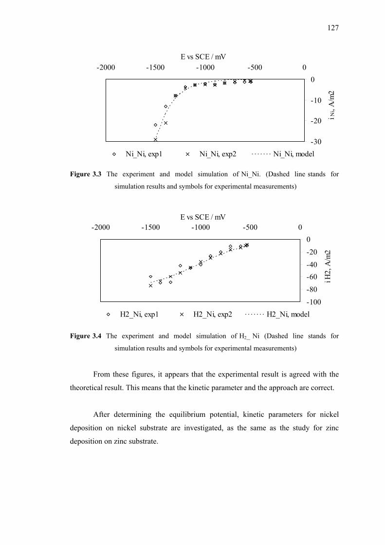
127

-30

-20

-10

0-2000 -1500 -1000 -500 0

E vs SCE / mV

i Ni,

A/m

2

Ni_Ni, exp1 Ni_Ni, exp2 Ni_Ni, model

Figure 3.3 The experiment and model simulation of Ni_Ni. (Dashed line stands for

simulation results and symbols for experimental measurements)

-100-80-60-40-200

-2000 -1500 -1000 -500 0E vs SCE / mV

i H2,

A/m

2

H2_Ni, exp1 H2_Ni, exp2 H2_Ni, model

Figure 3.4 The experiment and model simulation of H2_ Ni (Dashed line stands for

simulation results and symbols for experimental measurements)

From these figures, it appears that the experimental result is agreed with the

theoretical result. This means that the kinetic parameter and the approach are correct.

After determining the equilibrium potential, kinetic parameters for nickel

deposition on nickel substrate are investigated, as the same as the study for zinc

deposition on zinc substrate.

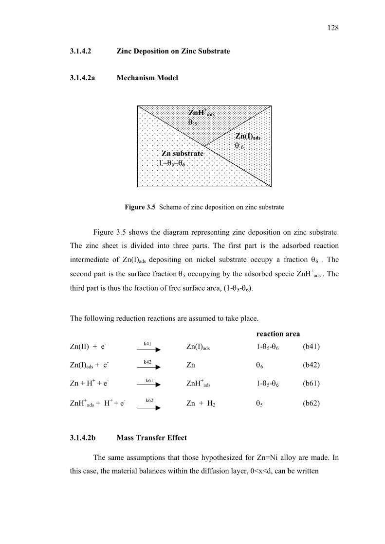
128

3.1.4.2 Zinc Deposition on Zinc Substrate


Figure 3.5 Scheme of zinc deposition on zinc substrate

Figure 3.5 shows the diagram representing zinc deposition on zinc substrate.

The zinc sheet is divided into three parts. The first part is the adsorbed reaction

intermediate of Zn(I)ads depositing on nickel substrate occupy a fraction θ6 . The

second part is the surface fraction θ5 occupying by the adsorbed specie ZnH+ads . The

third part is thus the fraction of free surface area, (1-θ5-θ6).


reaction area Zn(II) + e- k41 Zn(I)ads 1-θ5-θ6 (b41) Zn(I)ads + e- k42 Zn θ6 (b42) Zn + H+ + e- k61 ZnH+

ads 1-θ5-θ6 (b61) ZnH+

ads + H+ + e- k62 Zn + H2 θ5 (b62)


The same assumptions that those hypothesized for Zn=Ni alloy are made. In

this case, the material balances within the diffusion layer, 0<x<d, can be written

Zn(I)ads

θ 6

Zn substrate

1−θ5−θ6

ZnH+ads

θ 5

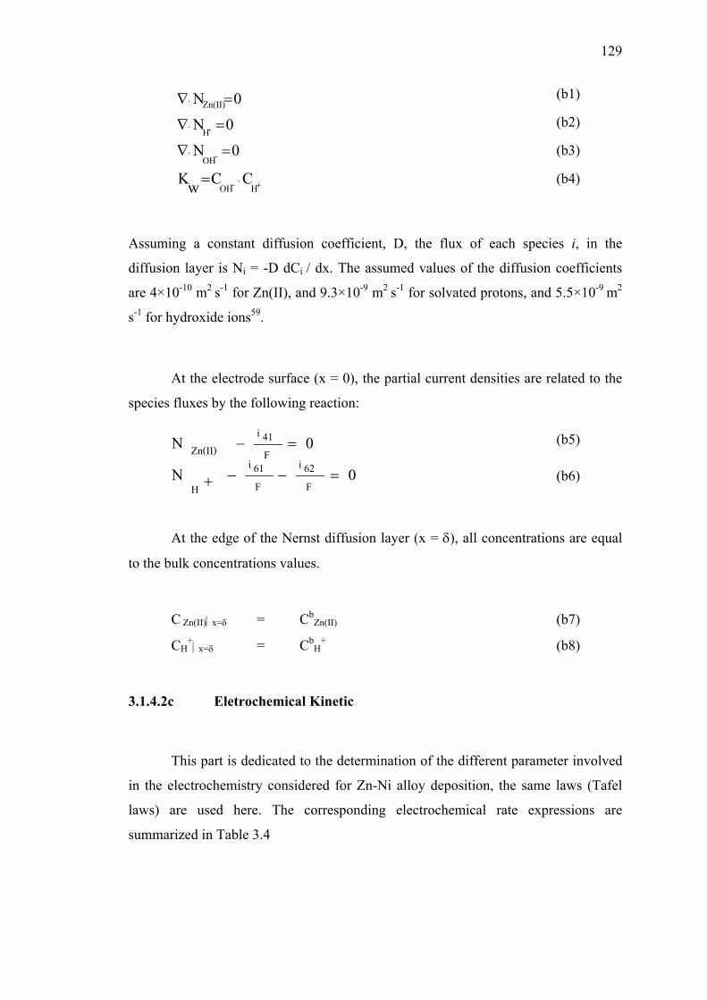
129

(b1)

(b2)

(b3)

(b4)



are 4×10-10 m2 s-1 for Zn(II), and 9.3×10-9 m2 s-1 for solvated protons, and 5.5×10-9 m2

s-1 for hydroxide ions59.


species fluxes by the following reaction:

(b5)

(b6)

At the edge of the Nernst diffusion layer (x = δ), all concentrations are equal

to the bulk concentrations values.

C Zn(II)x=δ = CbZn(II) (b7)

CH+

x=δ = CbH

+ (b8)

3.1.4.2c Eletrochemical Kinetic

This part is dedicated to the determination of the different parameter involved

in the electrochemistry considered for Zn-Ni alloy deposition, the same laws (Tafel



0N0N

F62i

F61i

H

F41i

Zn(II)=−−+

=−

+⋅−

−⋅

⋅

⋅

=

=∇

=∇

=∇

+

HOH

OH

H

Zn(II)

CCwK

0N

0N

0N

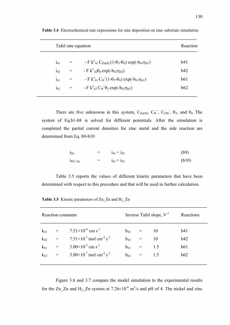
130

Table 3.4 Electrochemical rate expressions for zinc deposition on zinc substrate simulation


i41 = - F ko41 CZn(II) (1-θ5-θ6) exp(-b41η41) b41

i42 = - F kο42θ6 exp(-b42η42) b42

i61 = - F ko61 CH

+(1-θ5-θ6) exp(-b61η61) b61

i62 = - F kο62 CH

+θ5 exp(-b62η62) b62

There are five unknowns in this system, CZn(II), CH+, COH


system of Eq.b1-b8 is solved for different potentials. After the simulation is

completed the partial current densities for zinc metal and the side reaction are

determined from Eq. b9-b10

iZn = i41 + i42 (b9)

iH2/ Zn = i61 + i62 (b10)

Table 3.5 reports the values of different kinetic parameters that have been

determined with respect to this procedure and that will be used in further calculation.

Table 3.5 Kinetic parameters of Zn_Zn and H2_Zn


k41 = 7.51×10-6 cm s-1 b41 = 10 b41

k42 = 7.51×10 3 mol cm-2 s-1 b43 = 10 b42

k61 = 3.00×10-2 cm s-1 b61 = 1.5 b61

k62 = 3.00×10 7 mol cm-2 s-1 b62 = 1.5 b62

Figure 3.6 and 3.7 compare the model simulation to the experimental results

for the Zn_Zn and H2_Zn system at 7.26×10-6 m3/s and pH of 4. The nickel and zinc

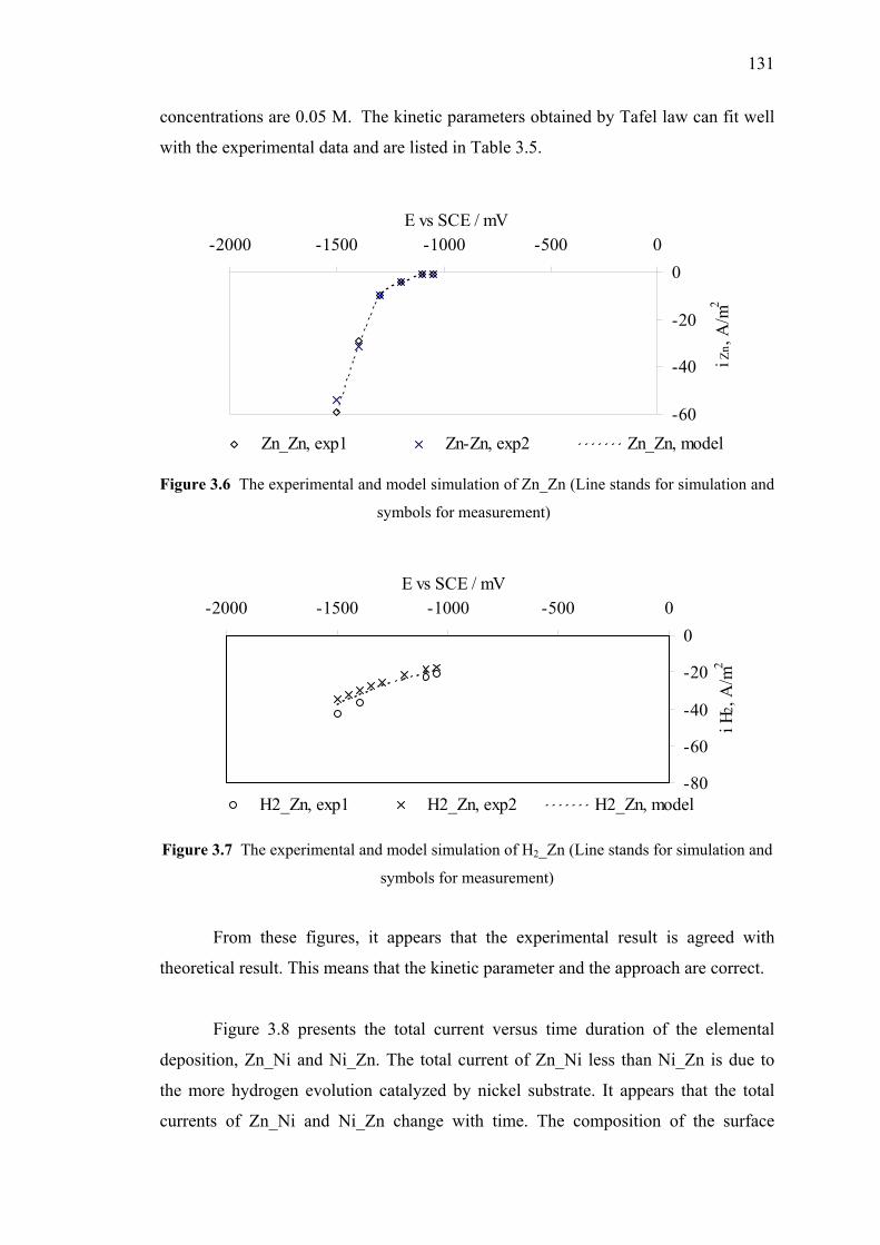
131

concentrations are 0.05 M. The kinetic parameters obtained by Tafel law can fit well

with the experimental data and are listed in Table 3.5.

-60

-40

-20

0-2000 -1500 -1000 -500 0

E vs SCE / mV

i Zn

, A/m

2

Zn_Zn, exp1 Zn-Zn, exp2 Zn_Zn, model

Figure 3.6 The experimental and model simulation of Zn_Zn (Line stands for simulation and

symbols for measurement)

-80

-60

-40

-20

0-2000 -1500 -1000 -500 0

E vs SCE / mV

i H2,

A/m

2

H2_Zn, exp1 H2_Zn, exp2 H2_Zn, model

Figure 3.7 The experimental and model simulation of H2_Zn (Line stands for simulation and


From these figures, it appears that the experimental result is agreed with


Figure 3.8 presents the total current versus time duration of the elemental

deposition, Zn_Ni and Ni_Zn. The total current of Zn_Ni less than Ni_Zn is due to

the more hydrogen evolution catalyzed by nickel substrate. It appears that the total

currents of Zn_Ni and Ni_Zn change with time. The composition of the surface

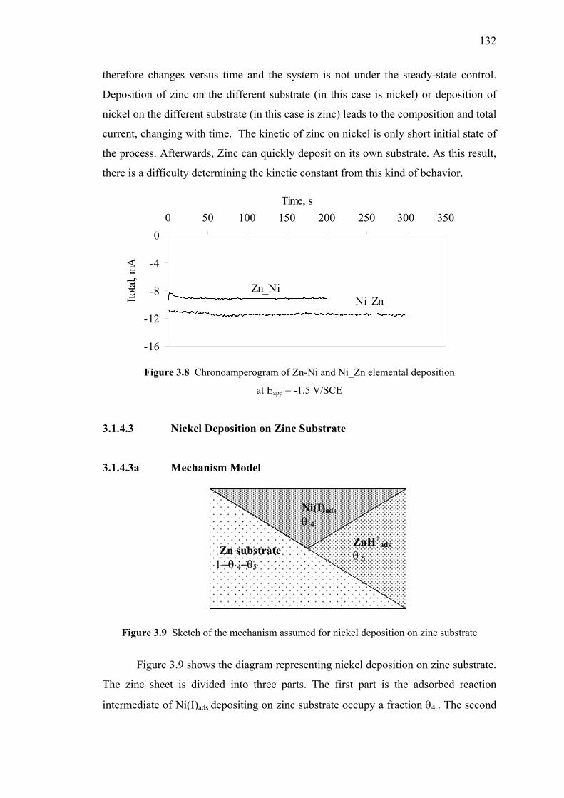
132

therefore changes versus time and the system is not under the steady-state control.

Deposition of zinc on the different substrate (in this case is nickel) or deposition of

nickel on the different substrate (in this case is zinc) leads to the composition and total

current, changing with time. The kinetic of zinc on nickel is only short initial state of

the process. Afterwards, Zinc can quickly deposit on its own substrate. As this result,

there is a difficulty determining the kinetic constant from this kind of behavior.

-16

-12

-8

-4

00 50 100 150 200 250 300 350

Time, s

Itota

l, m

A

Zn_NiNi_Zn

Figure 3.8 Chronoamperogram of Zn-Ni and Ni_Zn elemental deposition

at Eapp = -1.5 V/SCE

3.1.4.3 Nickel Deposition on Zinc Substrate


Figure 3.9 Sketch of the mechanism assumed for nickel deposition on zinc substrate

Figure 3.9 shows the diagram representing nickel deposition on zinc substrate.

The zinc sheet is divided into three parts. The first part is the adsorbed reaction

intermediate of Ni(I)ads depositing on zinc substrate occupy a fraction θ4 . The second

ZnH+ads

θ 5

Ni(I)adsθ 4

Zn substrate 1−θ 4−θ5

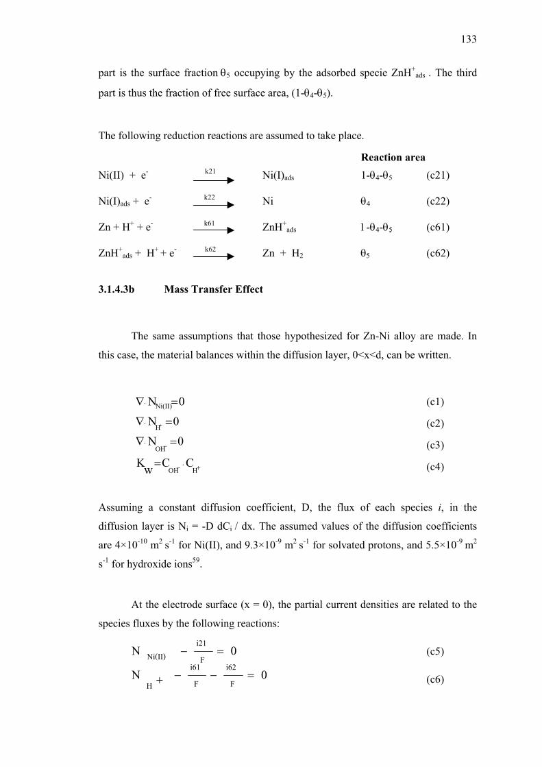
133

part is the surface fraction θ5 occupying by the adsorbed specie ZnH+ads . The third

part is thus the fraction of free surface area, (1-θ4-θ5).


Reaction area Ni(II) + e- k21 Ni(I)ads 1-θ4-θ5 (c21) Ni(I)ads + e- k22 Ni θ4 (c22) Zn + H+ + e- k61 ZnH+

ads 1-θ4-θ5 (c61)

ZnH+ads + H+ + e- k62 Zn + H2 θ5 (c62)


The same assumptions that those hypothesized for Zn-Ni alloy are made. In

this case, the material balances within the diffusion layer, 0<x<d, can be written.

(c1)

(c2)

(c3)

(c4)



are 4×10-10 m2 s-1 for Ni(II), and 9.3×10-9 m2 s-1 for solvated protons, and 5.5×10-9 m2



species fluxes by the following reactions:

(c5)

(c6) 0N0N

Fi62

Fi61

H

Fi21

Ni(II)=−−+

=−

+⋅−

−⋅

⋅

⋅

=

=∇

=∇

=∇

+

HOH

OH

H

Ni(II)

CCwK

0N

0N

0N

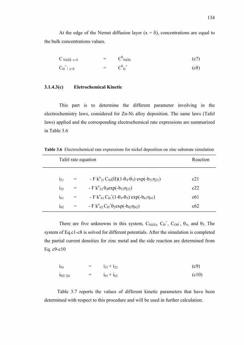
134

At the edge of the Nernst diffusion layer (x = δ), concentrations are equal to


C Ni(II)x=δ = CbNi(II) (c7)

CH+

x=δ = CbH

+ (c8)

3.1.4.3(c) Eletrochemical Kinetic

This part is to determine the different parameter involving in the

electrochemistry laws, considered for Zn-Ni alloy deposition. The same laws (Tafel

laws) applied and the corresponding electrochemical rate expressions are summarized

in Table 3.6

Table 3.6 Electrochemical rate expressions for nickel deposition on zinc substrate simulation


i21 = - F ko21 CNi(II)(1-θ4-θ5) exp(-b21η21) c21

i22 = - F kο22 θ4exp(-b22η22) c22

i61 = - F ko61 CH

+(1-θ4-θ5) exp(-b61η61) c61

i62 = - F kο62 CH

+θ5 exp(-b62η62) c62

There are five unknowns in this system, CNi(II), CH+, COH


system of Eq.c1-c8 is solved for different potentials. After the simulation is completed

the partial current densities for zinc metal and the side reaction are determined from

Eq. c9-c10

iNi = i21 + i22 (c9)

iH2/ Zn = i61 + i62 (c10)


determined with respect to this procedure and will be used in further calculation.

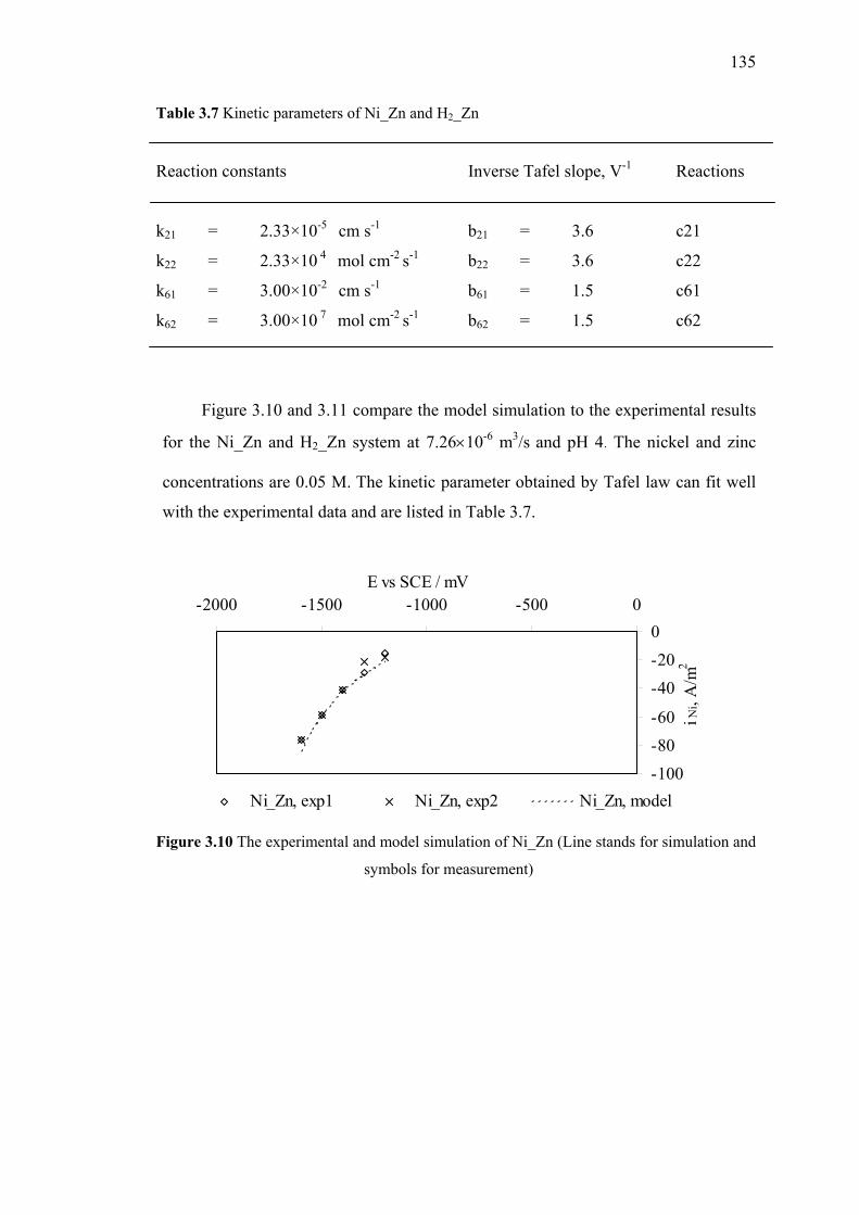
135

Table 3.7 Kinetic parameters of Ni_Zn and H2_Zn


k21 = 2.33×10-5 cm s-1 b21 = 3.6 c21

k22 = 2.33×10 4 mol cm-2 s-1 b22 = 3.6 c22

k61 = 3.00×10-2 cm s-1 b61 = 1.5 c61

k62 = 3.00×10 7 mol cm-2 s-1 b62 = 1.5 c62

Figure 3.10 and 3.11 compare the model simulation to the experimental results

for the Ni_Zn and H2_Zn system at 7.26×10-6 m3/s and pH 4. The nickel and zinc

concentrations are 0.05 M. The kinetic parameter obtained by Tafel law can fit well

with the experimental data and are listed in Table 3.7.

-100-80-60

-40-200

-2000 -1500 -1000 -500 0E vs SCE / mV

i Ni,

A/m

2

Ni_Zn, exp1 Ni_Zn, exp2 Ni_Zn, model

Figure 3.10 The experimental and model simulation of Ni_Zn (Line stands for simulation and


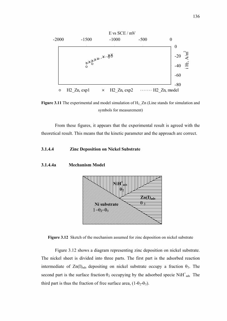
136

-80

-60

-40

-20

0-2000 -1500 -1000 -500 0

E vs SCE / mV

i H2,

A/m

2

H2_Zn, exp1 H2_Zn, exp2 H2_Zn, model

Figure 3.11 The experimental and model simulation of H2_Zn (Line stands for simulation and




3.1.4.4 Zinc Deposition on Nickel Substrate 3.1.4.4a Mechanism Model

Figure 3.12 Sketch of the mechanism assumed for zinc deposition on nickel substrate

Figure 3.12 shows a diagram representing zinc deposition on nickel substrate.

The nickel sheet is divided into three parts. The first part is the adsorbed reaction

intermediate of Zn(I)ads depositing on nickel substrate occupy a fraction θ3. The

second part is the surface fraction θ2 occupying by the adsorbed specie NiH+ads The

third part is thus the fraction of free surface area, (1-θ2-θ3).

NiHads θ 2

Zn(I)adsθ 3 Ni substrate

1−θ2−θ3

NiH+ads

θ2

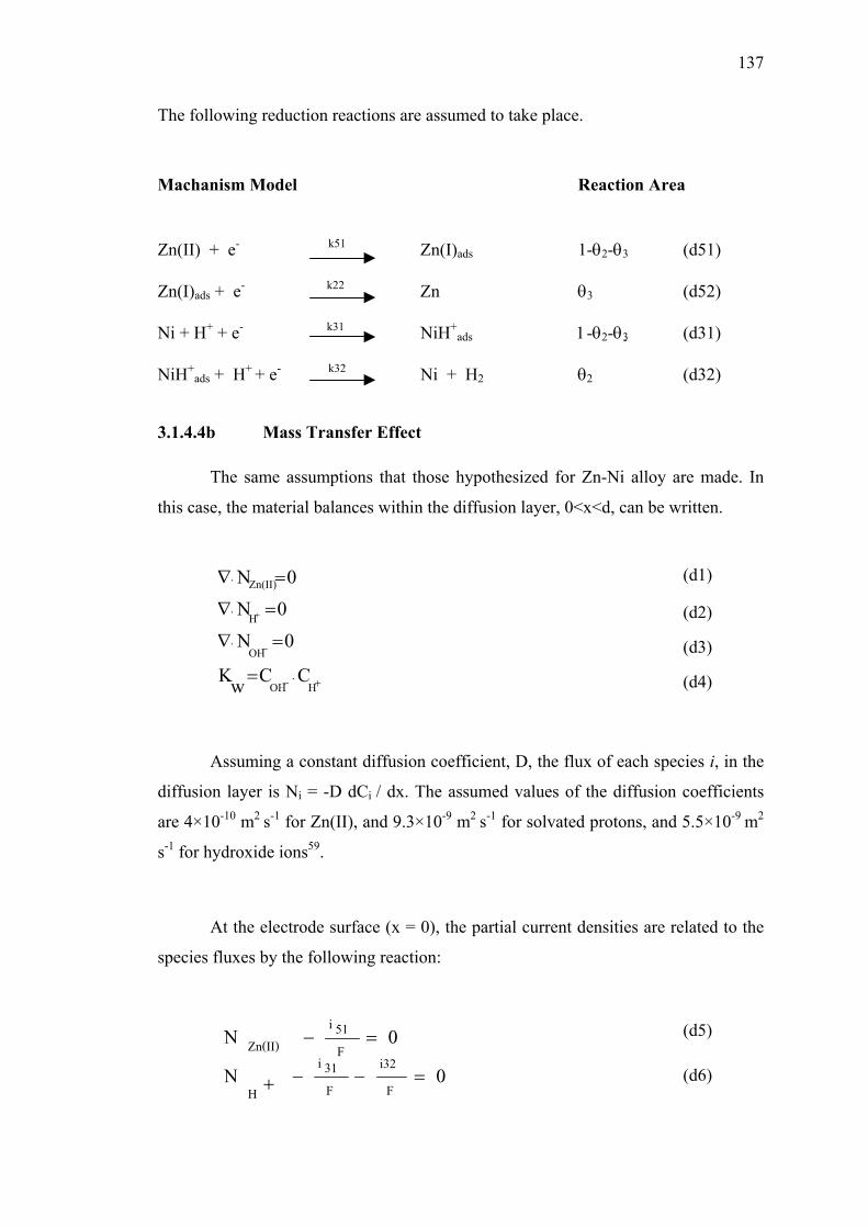
137


Machanism Model Reaction Area

Zn(II) + e- k51 Zn(I)ads 1-θ2-θ3 (d51) Zn(I)ads + e- k22 Zn θ3 (d52) Ni + H+ + e- k31 NiH+

ads 1-θ2-θ3 (d31)

NiH+ads + H+ + e- k32 Ni + H2 θ2 (d32)


The same assumptions that those hypothesized for Zn-Ni alloy are made. In

this case, the material balances within the diffusion layer, 0<x<d, can be written.

(d1)

(d2)

(d3)

(d4)



are 4×10-10 m2 s-1 for Zn(II), and 9.3×10-9 m2 s-1 for solvated protons, and 5.5×10-9 m2



species fluxes by the following reaction:

(d5)

(d6) 0N0N

Fi32

F31i

H

F51i

Zn(II)=−−+

=−

+⋅−

−⋅

⋅

⋅

=

=∇

=∇

=∇

+

HOH

OH

H

Zn(II)

CCwK

0N

0N

0N

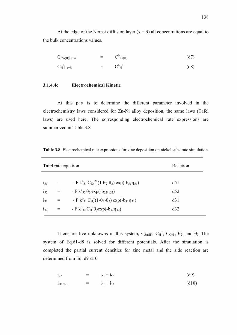
138

At the edge of the Nernst diffusion layer (x = δ) all concentrations are equal to


C Zn(II)x=δ = CbZn(II) (d7)

CH+

x=δ = CbH

+ (d8)

3.1.4.4c Electrochemical Kinetic

At this part is to determine the different parameter involved in the

electrochemistry laws considered for Zn-Ni alloy deposition, the same laws (Tafel



Table 3.8 Electrochemical rate expressions for zinc deposition on nickel substrate simulation


i51 = - F ko51 CZn

2+(1-θ2-θ3) exp(-b51η51) d51

i52 = - F kο52 θ3 exp(-b52η52) d52

i31 = - F ko31 CH

+(1-θ2-θ3) exp(-b31η31) d31

i32 = - F kο32 CH

+θ2 exp(-b32η32) d32

There are five unknowns in this system, CZn(II), CH+, COH


system of Eq.d1-d8 is solved for different potentials. After the simulation is

completed the partial current densities for zinc metal and the side reaction are

determined from Eq. d9-d10

iZn = i51 + i52 (d9)

iH2/ Ni = i31 + i32 (d10)

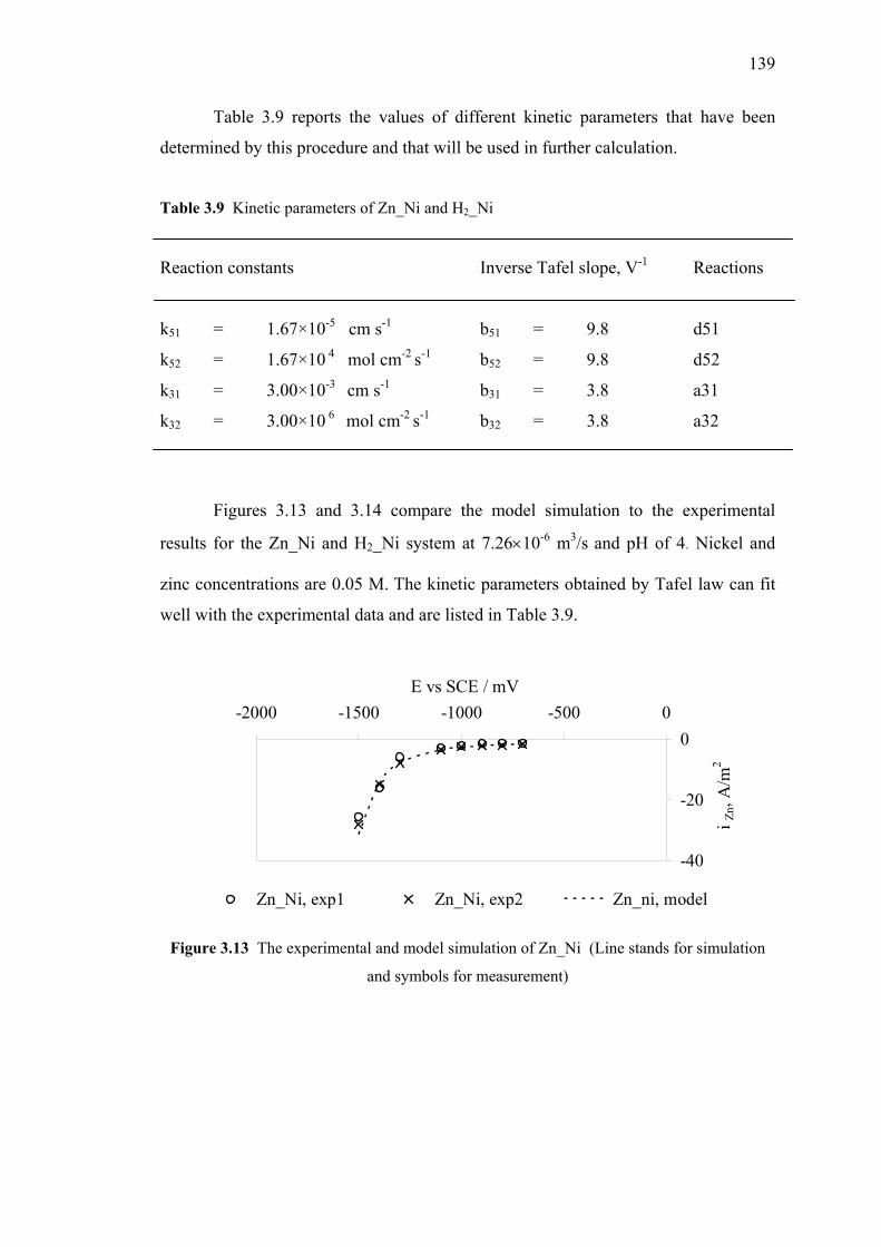
139


determined by this procedure and that will be used in further calculation.

Table 3.9 Kinetic parameters of Zn_Ni and H2_Ni


k51 = 1.67×10-5 cm s-1 b51 = 9.8 d51

k52 = 1.67×10 4 mol cm-2 s-1 b52 = 9.8 d52

k31 = 3.00×10-3 cm s-1 b31 = 3.8 a31

k32 = 3.00×10 6 mol cm-2 s-1 b32 = 3.8 a32

Figures 3.13 and 3.14 compare the model simulation to the experimental

results for the Zn_Ni and H2_Ni system at 7.26×10-6 m3/s and pH of 4. Nickel and

zinc concentrations are 0.05 M. The kinetic parameters obtained by Tafel law can fit

well with the experimental data and are listed in Table 3.9.

-40

-20

0-2000 -1500 -1000 -500 0

E vs SCE / mV

i Zn

, A/m

2

Zn_Ni, exp1 Zn_Ni, exp2 Zn_ni, model

Figure 3.13 The experimental and model simulation of Zn_Ni (Line stands for simulation

and symbols for measurement)

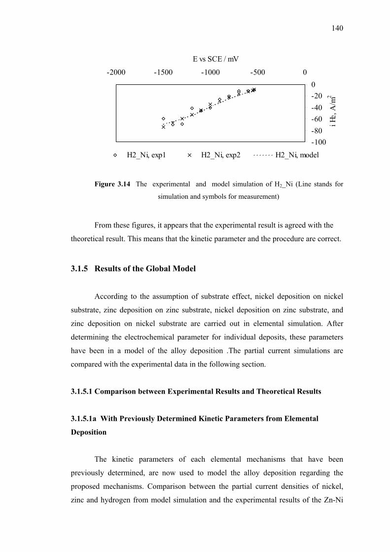
140

-100-80-60-40-200

-2000 -1500 -1000 -500 0

E vs SCE / mV

i H2,

A/m

2

H2_Ni, exp1 H2_Ni, exp2 H2_Ni, model

Figure 3.14 The experimental and model simulation of H2_Ni (Line stands for

simulation and symbols for measurement)


theoretical result. This means that the kinetic parameter and the procedure are correct.

3.1.5 Results of the Global Model

According to the assumption of substrate effect, nickel deposition on nickel

substrate, zinc deposition on zinc substrate, nickel deposition on zinc substrate, and

zinc deposition on nickel substrate are carried out in elemental simulation. After

determining the electrochemical parameter for individual deposits, these parameters

have been in a model of the alloy deposition .The partial current simulations are

compared with the experimental data in the following section.

3.1.5.1 Comparison between Experimental Results and Theoretical Results

3.1.5.1a With Previously Determined Kinetic Parameters from Elemental

Deposition

The kinetic parameters of each elemental mechanisms that have been

previously determined, are now used to model the alloy deposition regarding the

proposed mechanisms. Comparison between the partial current densities of nickel,

zinc and hydrogen from model simulation and the experimental results of the Zn-Ni

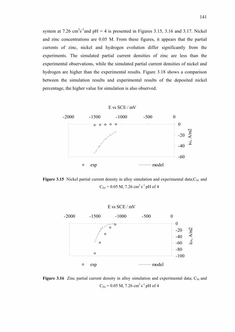
141

system at 7.26 cm3s-1and pH = 4 is presented in Figures 3.15, 3.16 and 3.17. Nickel

and zinc concentrations are 0.05 M. From these figures, it appears that the partial

currents of zinc, nickel and hydrogen evolution differ significantly from the

experiments. The simulated partial current densities of zinc are less than the

experimental observations, while the simulated partial current densities of nickel and

hydrogen are higher than the experimental results. Figure 3.18 shows a comparison

between the simulation results and experimental results of the deposited nickel

percentage, the higher value for simulation is also observed.

-60

-40

-20

0-2000 -1500 -1000 -500 0

E vs SCE / mV

iNi,

A/m

2

exp model

Figure 3.15 Nickel partial current density in alloy simulation and experimental data;CNi and

CZn = 0.05 M, 7.26 cm3 s-1 pH of 4

-100-80-60-40-200

-2000 -1500 -1000 -500 0

E vs SCE / mV

iZn, A

/m2

exp model

Figure 3.16 Zinc partial current density in alloy simulation and experimental data; CNi and

CZn = 0.05 M, 7.26 cm3 s-1 pH of 4

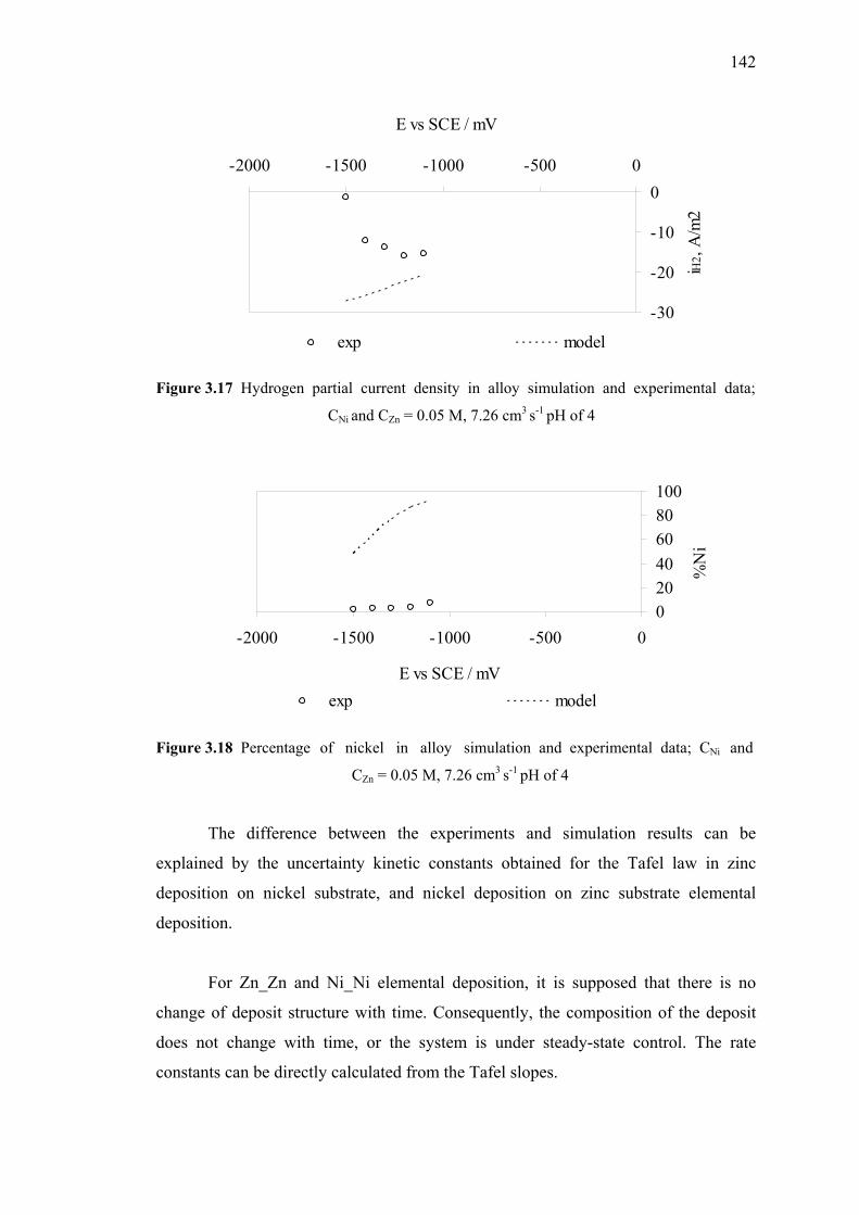
142

-30

-20

-10

0-2000 -1500 -1000 -500 0

E vs SCE / mV

iH2,

A/m

2

exp model

Figure 3.17 Hydrogen partial current density in alloy simulation and experimental data;

CNi and CZn = 0.05 M, 7.26 cm3 s-1 pH of 4

020406080100

-2000 -1500 -1000 -500 0

E vs SCE / mV%

Ni

exp model

Figure 3.18 Percentage of nickel in alloy simulation and experimental data; CNi and

CZn = 0.05 M, 7.26 cm3 s-1 pH of 4

The difference between the experiments and simulation results can be

explained by the uncertainty kinetic constants obtained for the Tafel law in zinc

deposition on nickel substrate, and nickel deposition on zinc substrate elemental

deposition.

For Zn_Zn and Ni_Ni elemental deposition, it is supposed that there is no

change of deposit structure with time. Consequently, the composition of the deposit

does not change with time, or the system is under steady-state control. The rate

constants can be directly calculated from the Tafel slopes.

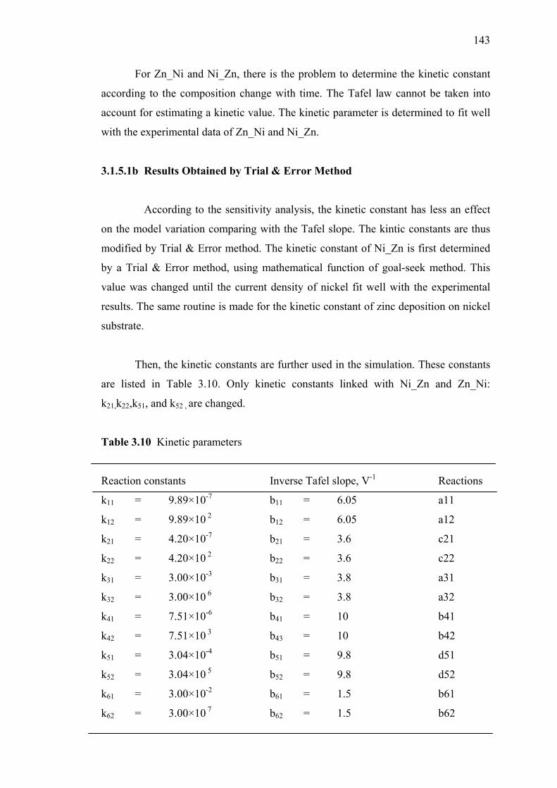
143

For Zn_Ni and Ni_Zn, there is the problem to determine the kinetic constant

according to the composition change with time. The Tafel law cannot be taken into

account for estimating a kinetic value. The kinetic parameter is determined to fit well

with the experimental data of Zn_Ni and Ni_Zn.

3.1.5.1b Results Obtained by Trial & Error Method

According to the sensitivity analysis, the kinetic constant has less an effect

on the model variation comparing with the Tafel slope. The kintic constants are thus

modified by Trial & Error method. The kinetic constant of Ni_Zn is first determined

by a Trial & Error method, using mathematical function of goal-seek method. This

value was changed until the current density of nickel fit well with the experimental

results. The same routine is made for the kinetic constant of zinc deposition on nickel

substrate.

Then, the kinetic constants are further used in the simulation. These constants

are listed in Table 3.10. Only kinetic constants linked with Ni_Zn and Zn_Ni:

k21,k22,k51, and k52 , are changed.

Table 3.10 Kinetic parameters


k11 = 9.89×10-7 b11 = 6.05 a11

k12 = 9.89×10 2 b12 = 6.05 a12

k21 = 4.20×10-7 b21 = 3.6 c21

k22 = 4.20×10 2 b22 = 3.6 c22

k31 = 3.00×10-3 b31 = 3.8 a31

k32 = 3.00×10 6 b32 = 3.8 a32

k41 = 7.51×10-6 b41 = 10 b41

k42 = 7.51×10 3 b43 = 10 b42

k51 = 3.04×10-4 b51 = 9.8 d51

k52 = 3.04×10 5 b52 = 9.8 d52

k61 = 3.00×10-2 b61 = 1.5 b61

k62 = 3.00×10 7 b62 = 1.5 b62

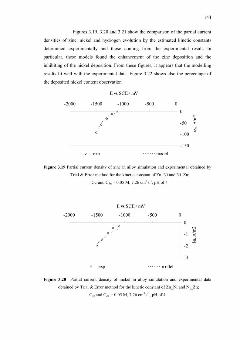
144

Figures 3.19, 3.20 and 3.21 show the comparison of the partial current

densities of zinc, nickel and hydrogen evolution by the estimated kinetic constants

determined experimentally and those coming from the experimental result. In

particular, these models found the enhancement of the zinc deposition and the

inhibiting of the nickel deposition. From these figures, it appears that the modelling

results fit well with the experimental data. Figure 3.22 shows also the percentage of

the deposited nickel content observation

-150

-100

-50

0-2000 -1500 -1000 -500 0

E vs SCE / mV

iZn, A

/m2

exp model

Figure 3.19 Partial current density of zinc in alloy simulation and experimental obtained by

Trial & Error method for the kinetic constant of Zn_Ni and Ni_Zn;

CNi and CZn = 0.05 M, 7.26 cm3 s-1, pH of 4

-3

-2

-1

0-2000 -1500 -1000 -500 0

E vs SCE / mV

iNi,

A/m

2

exp model

Figure 3.20 Partial current density of nickel in alloy simulation and experimental data

obtained by Trial & Error method for the kinetic constant of Zn_Ni and Ni_Zn;


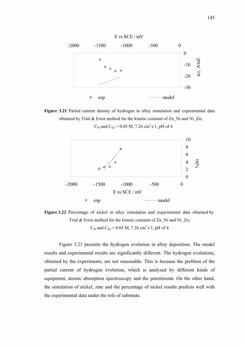
145

-30

-20

-10

0-2000 -1500 -1000 -500 0

E vs SCE / mV

iH2,

A/m

2

exp model

Figure 3.21 Partial current density of hydrogen in alloy simulation and experimental data

obtained by Trial & Error method for the kinetic constant of Zn_Ni and Ni_Zn;


0246810

-2000 -1500 -1000 -500 0E vs SCE / mV

%N

iexp model

Figure 3.22 Percentage of nickel in alloy simulation and experimental data obtained by

Trial & Error method for the kinetic constant of Zn_Ni and Ni_Zn;


Figure 3.21 presents the hydrogen evolution in alloy deposition. The model

results and experimental results are significantly different. The hydrogen evolutions,

obtained by the experiments, are not reasonable. This is because the problem of the

partial current of hydrogen evolution, which is analysed by different kinds of

equipment, atomic absorption spectroscopy and the potentiostat. On the other hand,

the simulation of nickel, zinc and the percentage of nickel results predicts well with

the experimental data under the role of substrate.

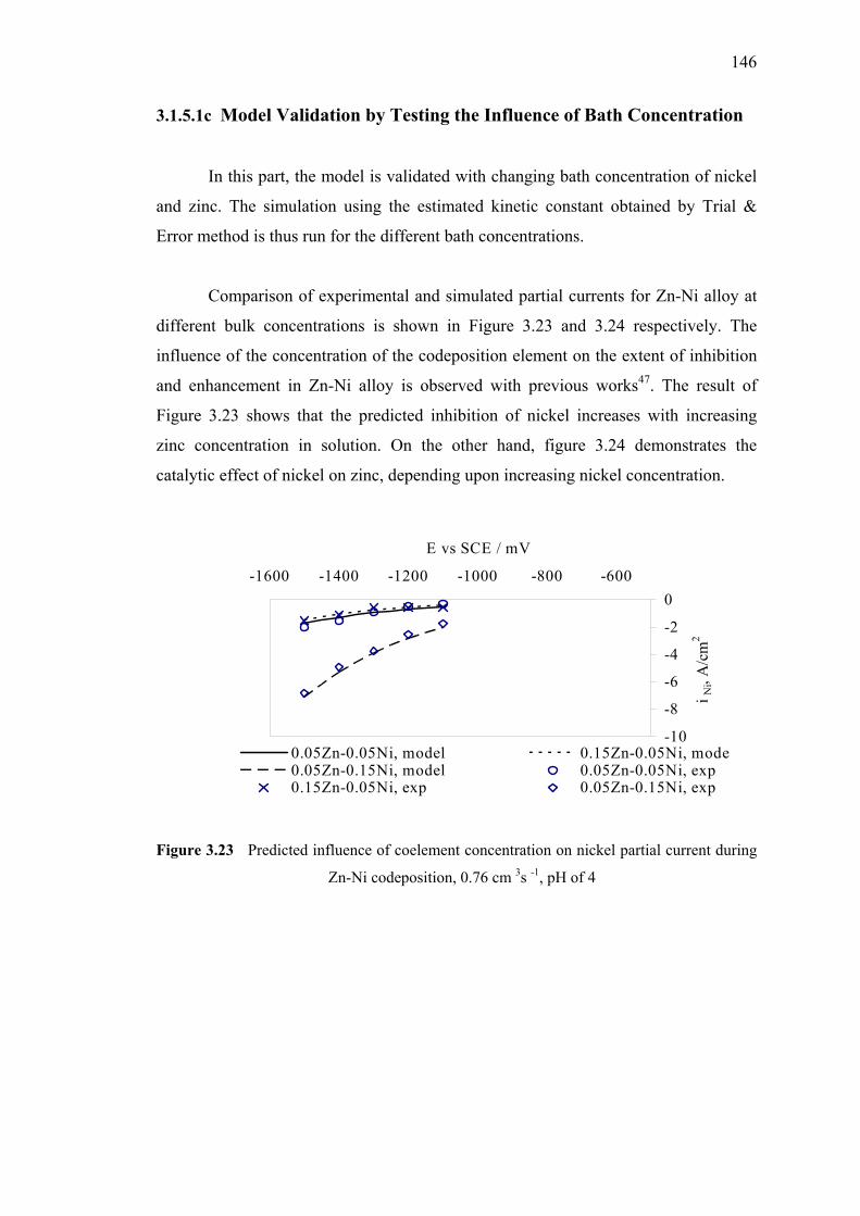
146

3.1.5.1c Model Validation by Testing the Influence of Bath Concentration

In this part, the model is validated with changing bath concentration of nickel

and zinc. The simulation using the estimated kinetic constant obtained by Trial &

Error method is thus run for the different bath concentrations.

Comparison of experimental and simulated partial currents for Zn-Ni alloy at

different bulk concentrations is shown in Figure 3.23 and 3.24 respectively. The

influence of the concentration of the codeposition element on the extent of inhibition

and enhancement in Zn-Ni alloy is observed with previous works47. The result of

Figure 3.23 shows that the predicted inhibition of nickel increases with increasing

zinc concentration in solution. On the other hand, figure 3.24 demonstrates the

catalytic effect of nickel on zinc, depending upon increasing nickel concentration.

-10

-8

-6

-4

-2

0-1600 -1400 -1200 -1000 -800 -600

E vs SCE / mV

i Ni,

A/c

m2

0.05Zn-0.05Ni, model 0.15Zn-0.05Ni, mode0.05Zn-0.15Ni, model 0.05Zn-0.05Ni, exp0.15Zn-0.05Ni, exp 0.05Zn-0.15Ni, exp

Figure 3.23 Predicted influence of coelement concentration on nickel partial current during

Zn-Ni codeposition, 0.76 cm 3s -1, pH of 4

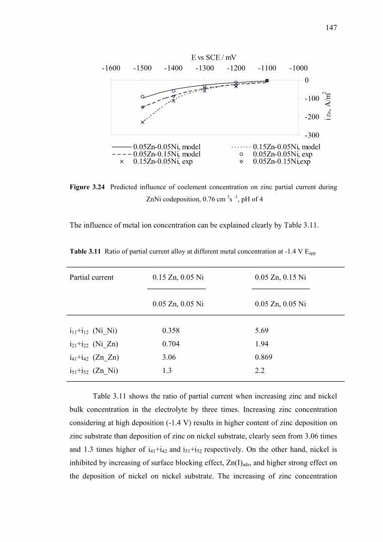
147

-300

-200

-100

0-1600 -1500 -1400 -1300 -1200 -1100 -1000

E vs SCE / mV

i Zn,

A/m

2

0.05Zn-0.05Ni, model 0.15Zn-0.05Ni, model0.05Zn-0.15Ni, model 0.05Zn-0.05Ni, exp0.15Zn-0.05Ni, exp 0.05Zn-0.15Ni,exp

Figure 3.24 Predicted influence of coelement concentration on zinc partial current during

ZnNi codeposition, 0.76 cm 3s -1, pH of 4

The influence of metal ion concentration can be explained clearly by Table 3.11.

Table 3.11 Ratio of partial current alloy at different metal concentration at -1.4 V Eapp

Partial current 0.15 Zn, 0.05 Ni 0.05 Zn, 0.15 Ni

0.05 Zn, 0.05 Ni 0.05 Zn, 0.05 Ni

i11+i12 (Ni_Ni) 0.358 5.69

i21+i22 (Ni_Zn) 0.704 1.94

i41+i42 (Zn_Zn) 3.06 0.869

i51+i52 (Zn_Ni) 1.3 2.2

Table 3.11 shows the ratio of partial current when increasing zinc and nickel

bulk concentration in the electrolyte by three times. Increasing zinc concentration

considering at high deposition (-1.4 V) results in higher content of zinc deposition on

zinc substrate than deposition of zinc on nickel substrate, clearly seen from 3.06 times

and 1.3 times higher of i41+i42 and i51+i52 respectively. On the other hand, nickel is

inhibited by increasing of surface blocking effect, Zn(I)ads, and higher strong effect on

the deposition of nickel on nickel substrate. The increasing of zinc concentration

148

therefore has a strong effect on enhancing rate of zinc deposition on zinc substrate and

inhibiting rate of nickel on nickel substrate.

Increasing nickel concentration results in higher content of nickel deposition

on nickel substrate than deposition of nickel on zinc substrate, clearly seen from 5.69

times and 1.94 times higher of i11+i12 and i21+i22 respectively. The result shows the

higher rate of zinc deposition that is able to deposit on nickel substrate as seen from

2.2 times higher of i51+i52. On the other hand, zinc is inhibited by increasing of surface

blocking effect, Ni(I)ads, but only the deposition of zinc on zinc substrate. Increasing

of nickel concentration therefore has a strong effect on enhancing rate of zinc

deposition on nickel substrate, nickel on nickel substrate and inhibiting rate of zinc on

zinc substrate.

3.1.6 Discussion

The present theoretical model gives a satisfactory description of observed

experimental results for different metal concentration of zinc and nickel. This

indicates that the basic physical assumptions underlying the model are reasonable.

According to the present model, the inhibition of the more noble metal, nickel, is due

to a surface blocking effect of adsorbed species similar to that described by Matlosz.

The enhancement of the deposition rate of the less noble metal, zinc, is attributed to

the catalyzing of zinc deposition current by nickel nuclei and the fresh nickel nuclei

that is the substrate related through Eq. 5a. The theoretical predictions depend

critically on the value of the kinetic contents, because the essential features of the

model lie on the kinetic expressions and adsorption effects at the surface. The kinetic

parameters for all reaction pathways can be obtained from single metal kinetics. The

model can therefore be used for the quantitative prediction of the effect of electrolyte

concentration on the resulting alloy composition. In addition, this model taking into

account the overpotential for determining the partial current by the Tafel equation.

The equilibrium potential depends on the substrate, which metal ions deposit on. The

equilibrium potentials of nickel, depositing on both nickel substrate and zinc

substrate, are -0.53 V. Conversely, the equilibrium potentials of zinc, depositing on

zinc substrate and nickel substrate, are different, as indicated -1.05 V and -0.07 V

149

respectively. The overpotentials in each partial current, in relation to substrate effect,

give more correct calculation of simulated partial currents.

3.1.7 Conclusion

The model entails a mathematical framework for the description of the

codeposition of Zn-Ni alloy lying on substrate effect for different electrolyte

concentration and applied potentials. The inhibition effect observed in nickel

deposition is attributed to the partial surface blocking by the adsorbed intermediates,

and the enhancing effect of zinc deposition is attributed to the catalyzing of zinc

deposition current by nickel nuclei. The model is able to simulate the influence of

potential, electrolyte concentration, and diffusion mass transport on the partial

currents and the resulting alloy codeposition.

Although it is found that the substrate model predicts well with the

experimental data. According to the experimental results of Zn-Ni alloy in chapter 2,

the mechanism model can be proposed in the role of mixed species effect. In the next

chapter, modelling the Zn-Ni mechanism under the role of mixed species will be

performed, as proposed by N. Zech. In this part, the model is modified in order to

predict the deposit content in the quantitative way.

150

3.2 Mixed Species Model

3.2.1 Introduction

In the first section of this chapter, the effect of substrate has been considered

for the modelling. As previously said, although the results of this model fit well with

the experimental evolution, there is no conclusive evidence that the nickel nuclei are

responsible for the enhancement of zinc deposition rate. Consequently, examining and

improving models with mixed species are taken into account. The experiment went

onto the modelling of Zn-Ni alloy, regarding the mixed species proposed by Wiart60

and later by Zech59. The partial currents of nickel, zinc and hydrogen are calculated as

a function of different bath concentrations. The partial currents determine the alloy

composition and current efficiency, which are compared to the experimental results.

3.2.2 Model Assumption

According to the experimental results in chapter 2, enhancing of zinc alloy

deposition and inhibiting of nickel alloy deposition, comparing with the elemental

deposition, are possible due to Zn-Ni mixed species. In this chapter, the mathematical

model describing the codeposition behaviour of nickel and zinc is therefore presented.

The model is essentially based on two general principles, as the following:

(1) Interfacial kinetics of the adsorbed species of nickel, zinc, Zn-Ni mixed

species, and hydrogen evolution on Zn-Ni substrate. In addition, the

adsorbed species can form at the electrode surface.

(2) Mass transport assuming a Nernst diffusion layer.

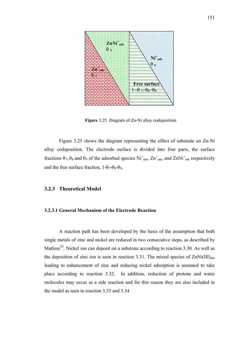
151

Figure 3.25 Diagram of Zn-Ni alloy codeposition

Figure 3.25 shows the diagram representing the effect of substrate on Zn-Ni

alloy codeposition. The electrode surface is divided into four parts, the surface

fractions θ7, θ8 and θ9 of the adsorbed species Ni+ads, Zn+

ads, and ZnNi+ads respectively

and the free surface fraction, 1-θ7-θ8-θ9.

3.2.3 Theoretical Model

3.2.3.1 General Mechanism of the Electrode Reaction

A reaction path has been developed by the basis of the assumption that both

single metals of zinc and nickel are reduced in two consecutive steps, as described by

Matlosz55. Nickel ion can deposit on a substrate according to reaction 3.30. As well as

the deposition of zinc ion is seen in reaction 3.31. The mixed species of ZnNi(III)ads

leading to enhancement of zinc and reducing nickel adsorption is assumed to take

place according to reaction 3.32. In addition, reduction of protons and water

molecules may occur as a side reaction and for this reason they are also included in

the model as seen in reaction 3.33 and 3.34

Zn+ads

θ 7

Ni+ads

θ 8

ZnNi+ads

θ 9

Free surface 1−θ 7−θ8−θ9

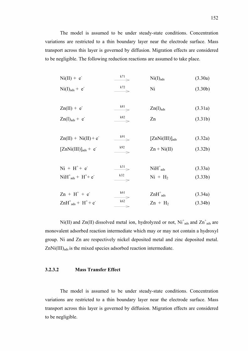
152

The model is assumed to be under steady-state conditions. Concentration

variations are restricted to a thin boundary layer near the electrode surface. Mass

transport across this layer is governed by diffusion. Migration effects are considered

to be negligible. The following reduction reactions are assumed to take place.


Ni(I)ads + e- k72 Ni (3.30b)


Zn(I)ads + e- k82 Zn (3.31b)

Zn(II) + Ni(II) + e- k91 [ZnNi(III)]ads (3.32a)

[ZnNi(III)]ads + e- k92 Zn + Ni(II) (3.32b)

Ni + H+ + e- k31 NiH+ads (3.33a)

NiH+ads + H++ e- k32 Ni + H2 (3.33b)

Zn + H+ + e- k61 ZnH+ads (3.34a)

ZnH+ads + H+ + e- k62 Zn + H2 (3.34b)

Ni(II) and Zn(II) dissolved metal ion, hydrolyzed or not, Ni+ads and Zn+

ads are

monovalent adsorbed reaction intermediate which may or may not contain a hydroxyl

group. Ni and Zn are respectively nickel deposited metal and zinc deposited metal.

ZnNi(III)ads is the mixed species adsorbed reaction intermediate.

3.2.3.2 Mass Transfer Effect

The model is assumed to be under steady-state conditions. Concentration

variations are restricted to a thin boundary layer near the electrode surface. Mass

transport across this layer is governed by diffusion. Migration effects are considered

to be negligible.

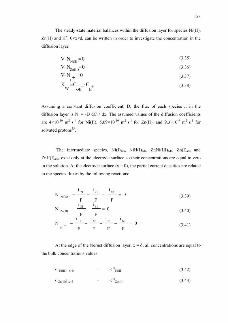
153

The steady-state material balances within the diffusion layer for species Ni(II),

Zn(II) and H+, 0<x<d, can be written in order to investigate the concentration in the

diffusion layer.

(3.35)

(3.36)

(3.37)

(3.38)



are 4×10-10 m2 s-1 for Ni(II), 5.09×10-10 m2 s-1 for Zn(II), and 9.3×10-9 m2 s-1 for

solvated protons35.

The intermediate species, Ni(I)ads, NiH(I)ads, ZnNi(III)ads, Zn(I)ads and

ZnH(I)ads, exist only at the electrode surface so their concentrations are equal to zero

in the solution. At the electrode surface (x = 0), the partial current densities are related

to the species fluxes by the following reactions:

(3.39)

(3.40)

(3.41)

At the edge of the Nernst diffusion layer, x = δ, all concentrations are equal to

the bulk concentrations values

C Ni(II) x=δ = CbNi(II) (3.42)

CZn(II) x=δ = Cb

Zn(II) (3.43)

+⋅−=

=+⋅∇=⋅∇=⋅∇

HOH

H

Zn(II)Ni(II)

CCwK0N0N0N

0F

iF

iF

iF

iN

0F

iF

iN

0F

iF

iF

iN

62613231H

9181Zn(II)

929171Ni(II)

=−−−−+

=−−

=−− −

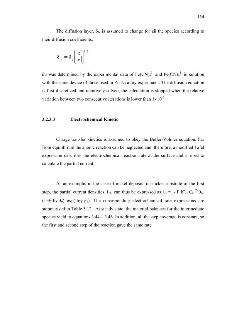
154

The diffusion layer, δN is assumed to change for all the species according to

their diffusion coefficients.

3/1

pND

= νδδ

δΝ was determined by the experimental data of Fe(CN)63- and Fe(CN)6

4- in solution

with the same device of those used in Zn-Ni alloy experiment. The diffusion equation

is first discretized and iteratively solved, the calculation is stopped when the relative

variation between two consecutive iterations is lower than 1×10-5.

3.2.3.3 Electrochemical Kinetic

Charge transfer kinetics is assumed to obey the Butler-Volmer equation. Far

from equilibrium the anodic reaction can be neglected and, therefore, a modified Tafel

expression describes the electrochemical reaction rate at the surface and is used to

calculate the partial current.

As an example, in the case of nickel deposits on nickel substrate of the first

step, the partial current densities, i71, can thus be expressed as i71 = - F ko71 CNi

2+θNi

(1-θ7-θ8-θ9) exp(-b71η71). The corresponding electrochemical rate expressions are

summarized in Table 3.12. At steady state, the material balances for the intermediate

species yield to equations 3.44 – 3.46. In addition, all the step coverage is constant, so

the first and second step of the reaction gave the same rate.

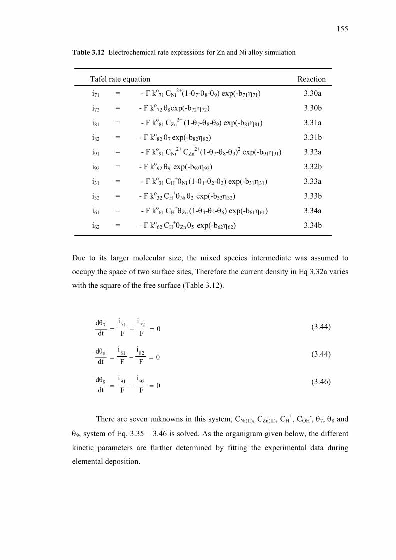
155

Table 3.12 Electrochemical rate expressions for Zn and Ni alloy simulation


i71 = - F ko71 CNi

2+(1-θ7-θ8-θ9) exp(-b71η71) 3.30a

i72 = - F kο72 θ8exp(-b72η72) 3.30b

i81 = - F ko81 CZn

2+ (1-θ7-θ8-θ9) exp(-b81η81) 3.31a

i82 = - F kο82 θ7 exp(-b82η82) 3.31b

i91 = - F ko91 CNi

2+ CZn

2+(1-θ7-θ8-θ9)2 exp(-b91η91) 3.32a

i92 = - F kο92 θ9 exp(-b92η92) 3.32b

i31 = - F ko31 CH

+θNi (1-θ1-θ2-θ3) exp(-b31η31) 3.33a

i32 = - F kο32 CH

+θNi θ2 exp(-b32η32) 3.33b

i61 = - F ko61 CH

+θZn (1-θ4-θ5-θ6) exp(-b61η61) 3.34a

i62 = - F kο62 CH

+θZn θ5 exp(-b62η62) 3.34b

Due to its larger molecular size, the mixed species intermediate was assumed to

occupy the space of two surface sites, Therefore the current density in Eq 3.32a varies

with the square of the free surface (Table 3.12).

(3.44)

(3.44)

(3.46)

There are seven unknowns in this system, CNi(II), CZn(II), CH

+, COH-, θ7, θ8 and

θ9, system of Eq. 3.35 – 3.46 is solved. As the organigram given below, the different

kinetic parameters are further determined by fitting the experimental data during

elemental deposition.

0F

i

F

i

dtθd

0F

i

F

i

dtθd

0F

i

F

i

dtdθ

92919

82818

72717

=−=

=−=

=−=

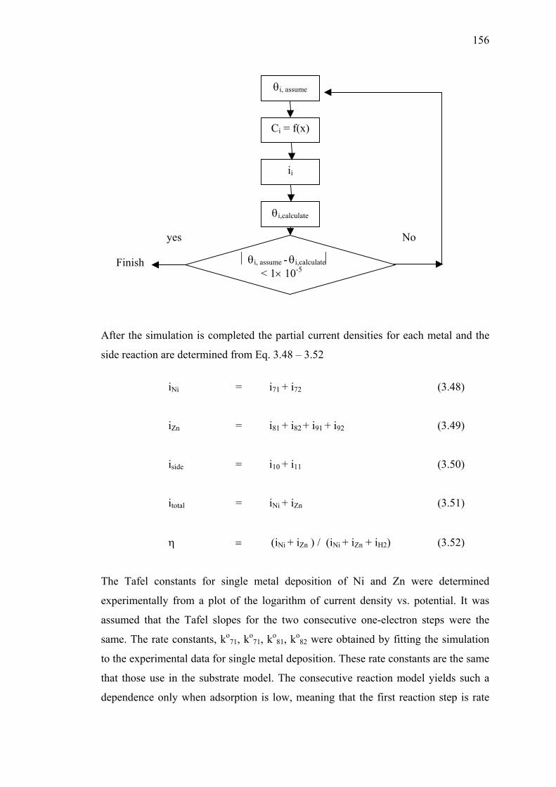
156

After the simulation is completed the partial current densities for each metal and the

side reaction are determined from Eq. 3.48 – 3.52

iNi = i71 + i72 (3.48) iZn = i81 + i82 + i91 + i92 (3.49) iside

= i10 + i11 (3.50) itotal = iNi + iZn (3.51) η = (iNi + iZn ) / (iNi + iZn + iH2) (3.52) The Tafel constants for single metal deposition of Ni and Zn were determined

experimentally from a plot of the logarithm of current density vs. potential. It was

assumed that the Tafel slopes for the two consecutive one-electron steps were the

same. The rate constants, ko71, ko

71, ko81, ko

82 were obtained by fitting the simulation

to the experimental data for single metal deposition. These rate constants are the same

that those use in the substrate model. The consecutive reaction model yields such a

dependence only when adsorption is low, meaning that the first reaction step is rate

θi, assume

Ci = f(x)

ii

θi,calculate

yes No

Finish θi, assume - θi,calculate < 1× 10-5

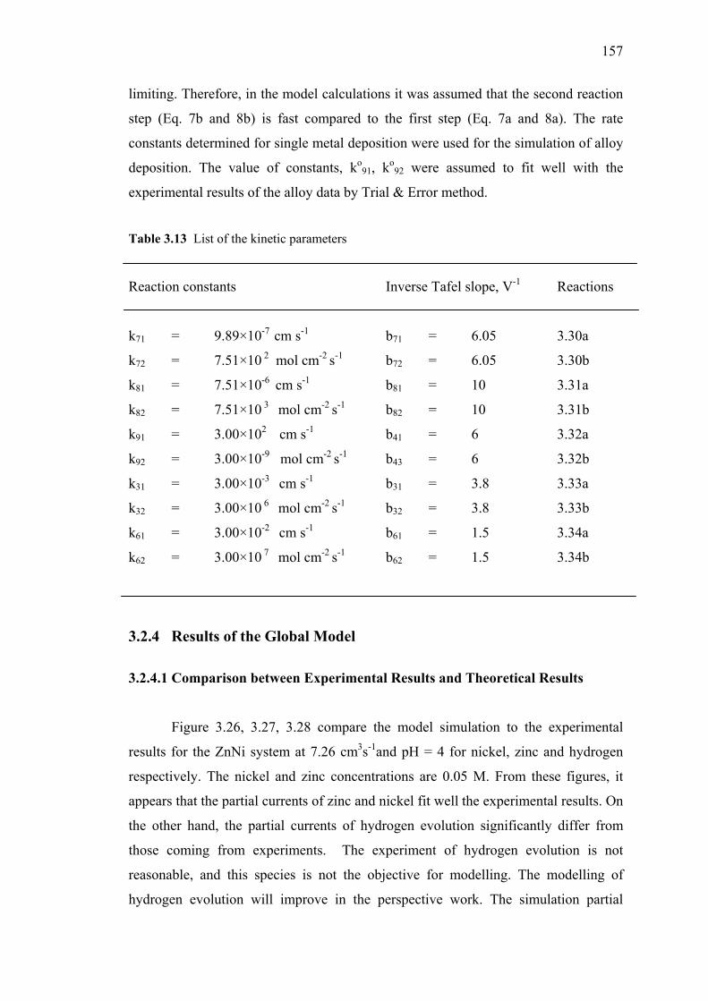
157

limiting. Therefore, in the model calculations it was assumed that the second reaction

step (Eq. 7b and 8b) is fast compared to the first step (Eq. 7a and 8a). The rate

constants determined for single metal deposition were used for the simulation of alloy

deposition. The value of constants, ko91, ko

92 were assumed to fit well with the

experimental results of the alloy data by Trial & Error method.

Table 3.13 List of the kinetic parameters


k71 = 9.89×10-7 cm s-1 b71 = 6.05 3.30a

k72 = 7.51×10 2 mol cm-2 s-1 b72 = 6.05 3.30b

k81 = 7.51×10-6 cm s-1 b81 = 10 3.31a

k82 = 7.51×10 3 mol cm-2 s-1 b82 = 10 3.31b

k91 = 3.00×102 cm s-1 b41 = 6 3.32a

k92 = 3.00×10-9 mol cm-2 s-1 b43 = 6 3.32b

k31 = 3.00×10-3 cm s-1 b31 = 3.8 3.33a

k32 = 3.00×10 6 mol cm-2 s-1 b32 = 3.8 3.33b

k61 = 3.00×10-2 cm s-1 b61 = 1.5 3.34a

k62 = 3.00×10 7 mol cm-2 s-1 b62 = 1.5 3.34b

3.2.4 Results of the Global Model

3.2.4.1 Comparison between Experimental Results and Theoretical Results

Figure 3.26, 3.27, 3.28 compare the model simulation to the experimental

results for the ZnNi system at 7.26 cm3s-1and pH = 4 for nickel, zinc and hydrogen

respectively. The nickel and zinc concentrations are 0.05 M. From these figures, it

appears that the partial currents of zinc and nickel fit well the experimental results. On

the other hand, the partial currents of hydrogen evolution significantly differ from

those coming from experiments. The experiment of hydrogen evolution is not

reasonable, and this species is not the objective for modelling. The modelling of

hydrogen evolution will improve in the perspective work. The simulation partial

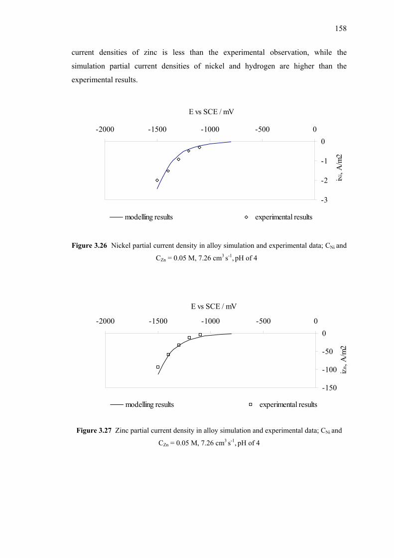
158

current densities of zinc is less than the experimental observation, while the

simulation partial current densities of nickel and hydrogen are higher than the

experimental results.

-3

-2

-1

0-2000 -1500 -1000 -500 0

E vs SCE / mV

iNi,

A/m

2

modelling results experimental results

Figure 3.26 Nickel partial current density in alloy simulation and experimental data; CNi and

CZn = 0.05 M, 7.26 cm3 s-1, pH of 4

-150

-100

-50

0-2000 -1500 -1000 -500 0

E vs SCE / mV

iZn, A

/m2

modelling results experimental results

Figure 3.27 Zinc partial current density in alloy simulation and experimental data; CNi and

CZn = 0.05 M, 7.26 cm3 s-1, pH of 4

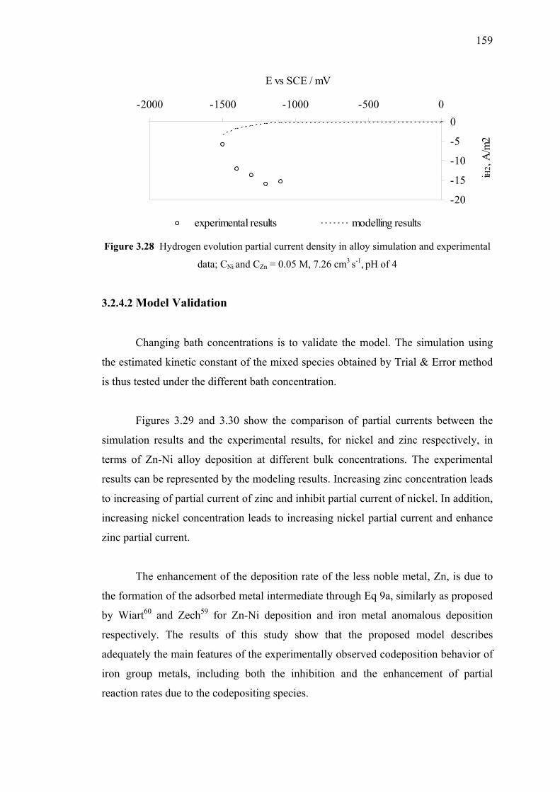
159

-20

-15

-10

-5

0-2000 -1500 -1000 -500 0

E vs SCE / mV

iH2,

A/m

2

experimental results modelling results

Figure 3.28 Hydrogen evolution partial current density in alloy simulation and experimental

data; CNi and CZn = 0.05 M, 7.26 cm3 s-1, pH of 4

3.2.4.2 Model Validation

Changing bath concentrations is to validate the model. The simulation using

the estimated kinetic constant of the mixed species obtained by Trial & Error method

is thus tested under the different bath concentration.

Figures 3.29 and 3.30 show the comparison of partial currents between the

simulation results and the experimental results, for nickel and zinc respectively, in

terms of Zn-Ni alloy deposition at different bulk concentrations. The experimental

results can be represented by the modeling results. Increasing zinc concentration leads

to increasing of partial current of zinc and inhibit partial current of nickel. In addition,

increasing nickel concentration leads to increasing nickel partial current and enhance

zinc partial current.

The enhancement of the deposition rate of the less noble metal, Zn, is due to

the formation of the adsorbed metal intermediate through Eq 9a, similarly as proposed

by Wiart60 and Zech59 for Zn-Ni deposition and iron metal anomalous deposition

respectively. The results of this study show that the proposed model describes

adequately the main features of the experimentally observed codeposition behavior of

iron group metals, including both the inhibition and the enhancement of partial

reaction rates due to the codepositing species.

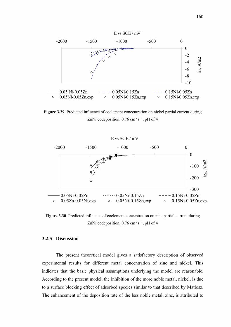
160

-10-8-6-4-20

-2000 -1500 -1000 -500 0

E vs SCE / mV

iNi,

A/m

2

0.05 Ni-0.05Zn 0.05Ni-0.15Zn 0.15Ni-0.05Zn0.05Ni-0.05Zn,exp 0.05Ni-0.15Zn,exp 0.15Ni-0.05Zn,exp

Figure 3.29 Predicted influence of coelement concentration on nickel partial current during


-300

-200

-100

0-2000 -1500 -1000 -500 0

E vs SCE / mV

iZn, A

/m2

0.05Ni-0.05Zn 0.05Ni-0.15Zn 0.15Ni-0.05Zn0.05Zn-0.05Ni,exp 0.05Ni-0.15Zn,exp 0.15Ni-0.05Zn,exp

Figure 3.30 Predicted influence of coelement concentration on zinc partial current during


3.2.5 Discussion

The present theoretical model gives a satisfactory description of observed

experimental results for different metal concentration of zinc and nickel. This

indicates that the basic physical assumptions underlying the model are reasonable.

According to the present model, the inhibition of the more noble metal, nickel, is due

to a surface blocking effect of adsorbed species similar to that described by Matlosz.

The enhancement of the deposition rate of the less noble metal, zinc, is attributed to

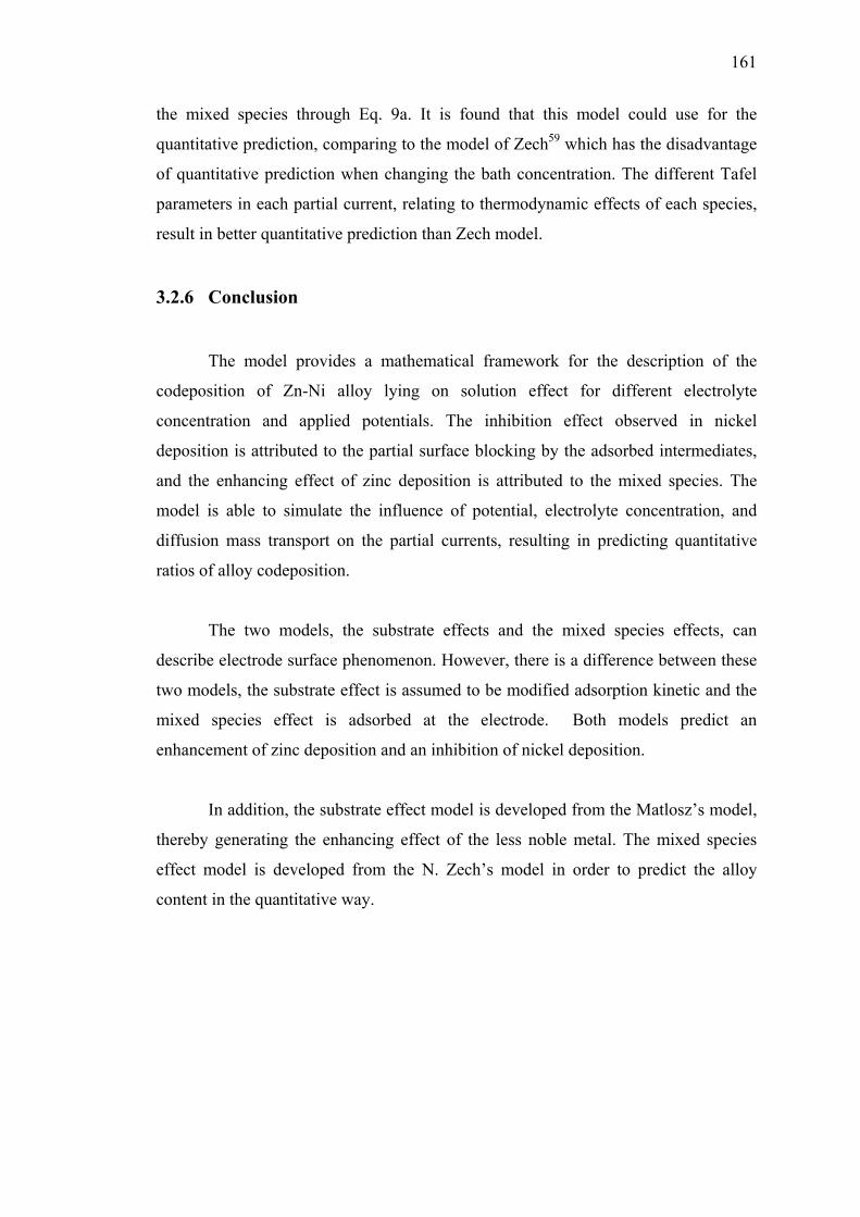
161

the mixed species through Eq. 9a. It is found that this model could use for the

quantitative prediction, comparing to the model of Zech59 which has the disadvantage

of quantitative prediction when changing the bath concentration. The different Tafel

parameters in each partial current, relating to thermodynamic effects of each species,

result in better quantitative prediction than Zech model.

3.2.6 Conclusion

The model provides a mathematical framework for the description of the

codeposition of Zn-Ni alloy lying on solution effect for different electrolyte

concentration and applied potentials. The inhibition effect observed in nickel

deposition is attributed to the partial surface blocking by the adsorbed intermediates,

and the enhancing effect of zinc deposition is attributed to the mixed species. The

model is able to simulate the influence of potential, electrolyte concentration, and

diffusion mass transport on the partial currents, resulting in predicting quantitative

ratios of alloy codeposition.

The two models, the substrate effects and the mixed species effects, can

describe electrode surface phenomenon. However, there is a difference between these

two models, the substrate effect is assumed to be modified adsorption kinetic and the

mixed species effect is adsorbed at the electrode. Both models predict an

enhancement of zinc deposition and an inhibition of nickel deposition.

In addition, the substrate effect model is developed from the Matlosz’s model,

thereby generating the enhancing effect of the less noble metal. The mixed species

effect model is developed from the N. Zech’s model in order to predict the alloy

content in the quantitative way.

162

3.3 Effect of Complexing Agent on Zn-Ni Alloy Deposition

3.3.1 Introduction

According to chapter 2 of the third part of this thesis, the experimental

investigation and mathematical modeling of Zn-Ni alloy electrodeposition have been

carried out. In this part, the complexing agent imposing on the Zn-Ni alloy

mechanism is focused. Consequently, the electrodeposition of Zn-Ni alloy from

potassium chloride bath under potentiostatic mode was studied in order to enhance

knowledge of this process and to establish a mathematical model of complexing agent

effect on Zn-Ni alloy deposition.

Comprehensive studies have been carried out on such electrodepositions from

different baths, including cyanide1, sulfate2-3 and chloride baths 4-6. In recent years,

there has been a preference for chloride-based solutions since it is probably easier to

obtain NiCl precipitation of 10%-15%, nickel-containing layers. Some of these

chloride electrolytes also contain other species acting as a buffer and / or complexing

agent, such as boric acid38-40, acetic acid44, 45 or ammonium chloride41, 46. Now, the

alkaline bath developed by Muller is preferred and mainly used for corrosion

protection.

From the assumption of the anomalous behavior is attributed to the formation

of a zinc hydroxide film on the electrode surface, which suppresses the discharge of

nickel ions. The zinc hydroxide formation arises from the local increase in pH due to

the hydrogen reduction. Presence of NH4Cl in the chloride bath therefore prevents the

precipitation of zinc hydroxide and increases the reduction of nickel, and then

increases the nickel content in the deposit. This suggests the formation of ammonium

complexes, such as [Zn(NH3)4]2+ and [Ni(NH3)6]2+ which prevent hydroxide

precipitation47.

The other assumption of chloride bath is the adsorption of chloride ion, Cl- and

the chloride complex. Zinc can be complex by chloride such as [ZnCl+], [ZnCl2],

[ZnCl-3] and [ZnCl2-

4], while nickel is not complex by chloride ion. This chloride

163

complexing behavior of zinc is also able to increase more nickel depositing on the

electrode surface48.

The objective of this work is to model Zn-Ni alloy deposition, which takes

into account the role of complexing effect of chloride ion comparing with the

experiment of KCl bath. The salt, KCl has been used in Zn-Ni deposition and

investigated how it can affect the system. Consequently, this study is the previous

proposal dealing with how the salt involves in the complexing effect.

3.3.2 Experiment

Experiments are carried out with an EQCM. The alloy content is determined

by atomic adsorption spectroscopy. The electroplating solution contained 0.05 mole

dm-3 ZnCl2, 0.05 mole dm-3 , NiCl2 6H2O for the bath with no complexing agent

effect. In order to study the effect of complexing agent, KCl 1 and 2 mole dm-3 is

added to the electrolyte. The pH of the electrolyte is kept constantly at pH 4.

The alloys are obtained at 25 ºC by depositing the metals potentiostatically

onto the crystal quartz gold electrode with a diameter of 1.37 cm2. The electrolyte

flow rate is 0.76 cm 3s -1. The reference electrode is the saturated calomel electrode,

and a platinum mesh is used as a counter electrode.

3.3.3 Results and Discussions

Figure 3.31 shows the current – time dependence for the deposition of Zn-Ni

alloy comparing with and without KCl complexing agent at -1.4 V of applied

potential. The increase of total current resulted only from adding KCl,

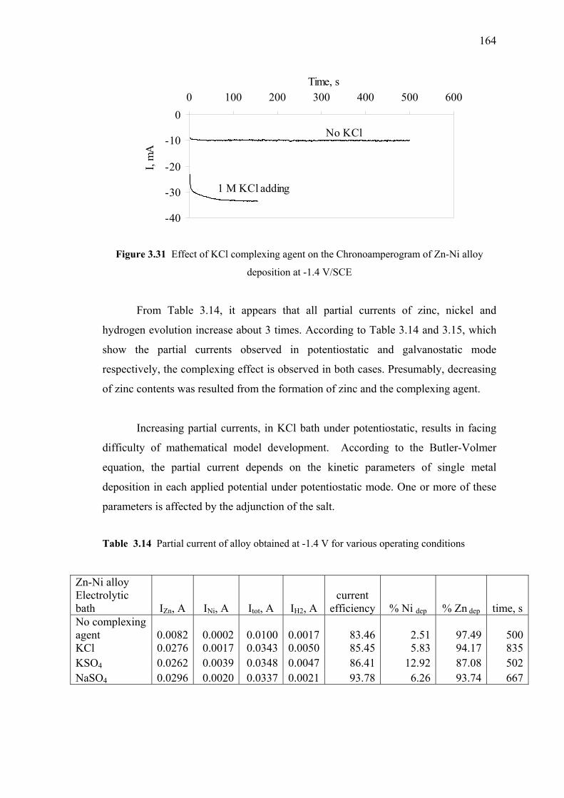
164

-40

-30

-20

-10

00 100 200 300 400 500 600

Time, s

I, m

A

1 M KCl adding

No KCl

Figure 3.31 Effect of KCl complexing agent on the Chronoamperogram of Zn-Ni alloy

deposition at -1.4 V/SCE

From Table 3.14, it appears that all partial currents of zinc, nickel and

hydrogen evolution increase about 3 times. According to Table 3.14 and 3.15, which

show the partial currents observed in potentiostatic and galvanostatic mode

respectively, the complexing effect is observed in both cases. Presumably, decreasing

of zinc contents was resulted from the formation of zinc and the complexing agent.

Increasing partial currents, in KCl bath under potentiostatic, results in facing

difficulty of mathematical model development. According to the Butler-Volmer

equation, the partial current depends on the kinetic parameters of single metal

deposition in each applied potential under potentiostatic mode. One or more of these

parameters is affected by the adjunction of the salt.

Table 3.14 Partial current of alloy obtained at -1.4 V for various operating conditions

Zn-Ni alloy Electrolytic bath IZn, A INi, A Itot, A IH2, A

current efficiency % Ni dep % Zn dep time, s

No complexing agent 0.0082 0.0002 0.0100 0.0017 83.46 2.51 97.49 500KCl 0.0276 0.0017 0.0343 0.0050 85.45 5.83 94.17 835KSO4 0.0262 0.0039 0.0348 0.0047 86.41 12.92 87.08 502NaSO4 0.0296 0.0020 0.0337 0.0021 93.78 6.26 93.74 667

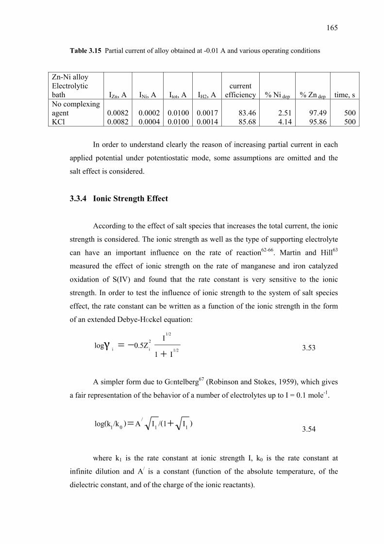
165

Table 3.15 Partial current of alloy obtained at -0.01 A and various operating conditions

Zn-Ni alloy Electrolytic bath IZn, A INi, A Itot, A IH2, A

current efficiency % Ni dep % Zn dep time, s

No complexing agent 0.0082 0.0002 0.0100 0.0017 83.46 2.51 97.49 500KCl 0.0082 0.0004 0.0100 0.0014 85.68 4.14 95.86 500

In order to understand clearly the reason of increasing partial current in each

applied potential under potentiostatic mode, some assumptions are omitted and the

salt effect is considered.

3.3.4 Ionic Strength Effect

According to the effect of salt species that increases the total current, the ionic

strength is considered. The ionic strength as well as the type of supporting electrolyte

can have an important influence on the rate of reaction62-66. Martin and Hill63

measured the effect of ionic strength on the rate of manganese and iron catalyzed

oxidation of S(IV) and found that the rate constant is very sensitive to the ionic

strength. In order to test the influence of ionic strength to the system of salt species

effect, the rate constant can be written as a function of the ionic strength in the form

of an extended Debye-HÜckel equation:

1/2

1/22ii I1

I0.5Zlogγ+

−= 3.53

A simpler form due to GÜntelberg67 (Robinson and Stokes, 1959), which gives

a fair representation of the behavior of a number of electrolytes up to I = 0.1 mole-1.

)I/(1IA)/klog(k 11/

01 += 3.54

where k1 is the rate constant at ionic strength I, k0 is the rate constant at

infinite dilution and A/ is a constant (function of the absolute temperature, of the

dielectric constant, and of the charge of the ionic reactants).

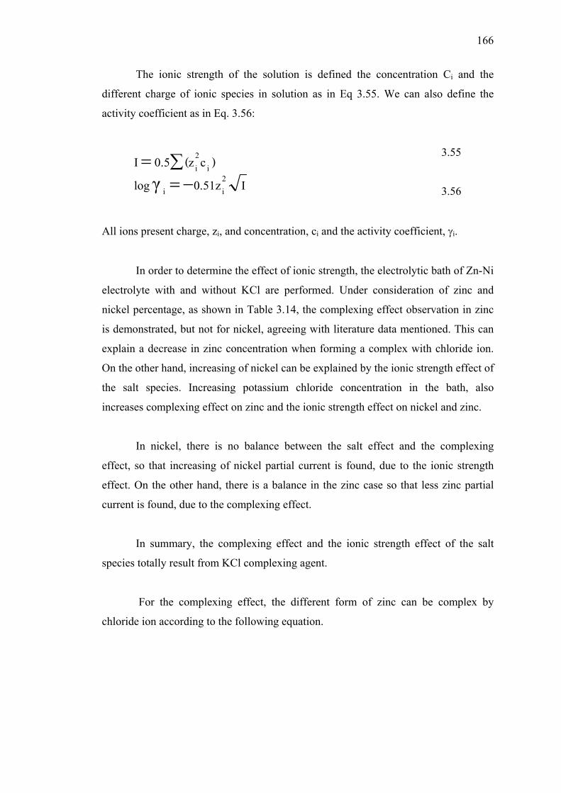
166

The ionic strength of the solution is defined the concentration Ci and the

different charge of ionic species in solution as in Eq 3.55. We can also define the

activity coefficient as in Eq. 3.56:

3.55

3.56

All ions present charge, zi, and concentration, ci and the activity coefficient, γi.

In order to determine the effect of ionic strength, the electrolytic bath of Zn-Ni

electrolyte with and without KCl are performed. Under consideration of zinc and

nickel percentage, as shown in Table 3.14, the complexing effect observation in zinc

is demonstrated, but not for nickel, agreeing with literature data mentioned. This can

explain a decrease in zinc concentration when forming a complex with chloride ion.

On the other hand, increasing of nickel can be explained by the ionic strength effect of

the salt species. Increasing potassium chloride concentration in the bath, also

increases complexing effect on zinc and the ionic strength effect on nickel and zinc.

In nickel, there is no balance between the salt effect and the complexing

effect, so that increasing of nickel partial current is found, due to the ionic strength

effect. On the other hand, there is a balance in the zinc case so that less zinc partial

current is found, due to the complexing effect.

In summary, the complexing effect and the ionic strength effect of the salt

species totally result from KCl complexing agent.

For the complexing effect, the different form of zinc can be complex by

chloride ion according to the following equation.

Iz51.0log)cz(5.0I

2ii

i2i

−=∑=

γ

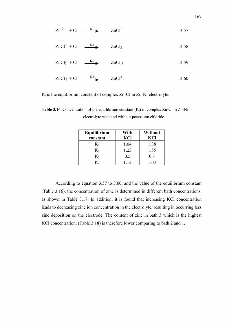
167

Zn 2+ + Cl - K1 ZnCl+ 3.57

ZnCl+ + Cl- K2 ZnCl2 3.58

ZnCl2 + Cl- K3 ZnCl-3 3.59

ZnCl-3 + Cl- K4 ZnCl2-

4 3.60

Ki is the equilibrium constant of complex Zn-Cl in Zn-Ni electrolyte.

Table 3.16 Concentration of the equilibrium constant (Ki) of complex Zn-Cl in Zn-Ni

electrolyte with and without potassium chloride

Equilibrium constant

With KCl

Without KCl

K1 1.04 1.38 K2 1.25 1.55 K3 0.5 0.3 K4 1.13 1.03

According to equation 3.57 to 3.60, and the value of the equilibrium constant

(Table 3.16), the concentration of zinc is determined in different bath concentrations,

as shown in Table 3.17. In addition, it is found that increasing KCl concentration

leads to decreasing zinc ion concentration in the electrolyte, resulting in occurring less

zinc deposition on the electrode. The content of zinc in bath 3 which is the highest

KCl concentration, (Table 3.18) is therefore lower comparing to bath 2 and 1.

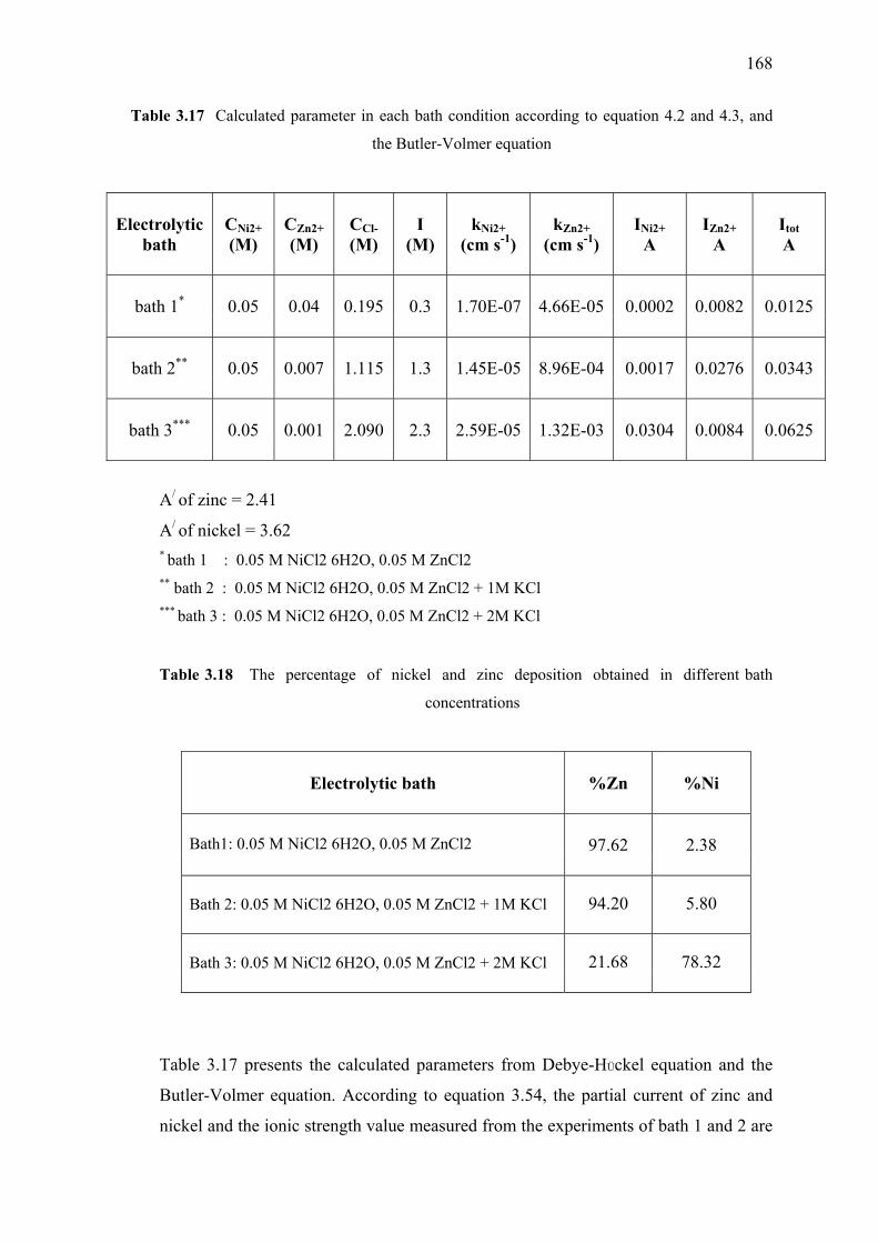
168

Table 3.17 Calculated parameter in each bath condition according to equation 4.2 and 4.3, and

the Butler-Volmer equation

Electrolytic

bath

CNi2+ (M)

CZn2+ (M)

CCl-(M)

I (M)

kNi2+ (cm s-1)

kZn2+ (cm s-1)

INi2+ A

IZn2+ A

Itot A

bath 1*

0.05

0.04

0.195

0.3

1.70E-07

4.66E-05

0.0002

0.0082

0.0125

bath 2**

0.05

0.007

1.115

1.3

1.45E-05

8.96E-04

0.0017

0.0276

0.0343

bath 3***

0.05

0.001

2.090

2.3

2.59E-05

1.32E-03

0.0304

0.0084

0.0625

A/ of zinc = 2.41

A/ of nickel = 3.62 * bath 1 : 0.05 M NiCl2 6H2O, 0.05 M ZnCl2 ** bath 2 : 0.05 M NiCl2 6H2O, 0.05 M ZnCl2 + 1M KCl *** bath 3 : 0.05 M NiCl2 6H2O, 0.05 M ZnCl2 + 2M KCl

Table 3.18 The percentage of nickel and zinc deposition obtained in different bath

concentrations

Electrolytic bath

%Zn

%Ni

97.62 2.38

Bath1: 0.05 M NiCl2 6H2O, 0.05 M ZnCl2

Bath 2: 0.05 M NiCl2 6H2O, 0.05 M ZnCl2 + 1M KCl 94.20 5.80

Bath 3: 0.05 M NiCl2 6H2O, 0.05 M ZnCl2 + 2M KCl 21.68 78.32

Table 3.17 presents the calculated parameters from Debye-HÜckel equation and the

Butler-Volmer equation. According to equation 3.54, the partial current of zinc and

nickel and the ionic strength value measured from the experiments of bath 1 and 2 are

169

used to calculate the kinetic parameters and A/ of zinc and nickel. These parameters

are then used to calculate the partial current of nickel and zinc for the bath 3.

In order to prove the effect of the ionic strength, in bath 3 condition, the partial

currents of zinc and nickel are determined by Butler-Volmer equation as shown in

Table 3.1, Part 3. The kinetic parameters of zinc and nickel in the Butler-Volmer

equation are calculated by equation 3.54, whereas the ionic strength is determined

from the experiments. The concentration of zinc used in the Butler-Volmer equation

is calculated with respect to the complexing effect. As mentioned above, the

summation of zinc and nickel partial current from the calculation is not exceed the

total current. The ionic strength effect and the complexing effect by KCl are thus able

to explain this behavior.

According to Table 3.17, the rate constant of zinc and nickel calculated by the

Debye-HÜckel equation is increased, in accordance with an increase of added KCl

concentration. This can be explained that salt species has an effect on catalyzing rate

of zinc and nickel deposition in Zn-Ni electrolyte. On the other hand, there is the

complexing effect of chloride ion on zinc. Decreasing of zinc and increasing of nickel

content on the deposit, shown in Table 3.18, are therefore due to the complexing

effect and the ionic strength effect respectively.

3.3.5 Conclusion

According to the assumption, the complexing agent is able to form a complex

with zinc ion in the solution in many forms with chloride ion, while nickel is not

complexed by chloride ion. There is an increase of complexing effect to zinc with

respect to increasing KCl concentration in the bath, while no effect on nickel.

Decreasing of zinc content on the deposit is thus explained by the complexing effect.

On the other hand, increasing nickel leads to more nickel on the deposit, and can be

explained by the ionic strength of the salt species. This work is the first research

studies investigating the salt effect on the growth rate of Zn-Ni alloy. It is

recommended that the further study should be conducted and followed in the

perspective work.

GENERAL CONCLUSION

This research devoted to the analysis of the electrochemical reactors. A multi-

scale approach, from the macroscale to the microscale, was applied. At the first stage,

macroscopic scale application is geared towards predicting a link between the outlet

reactor and the inlet reactor, depending upon the operating conditions. This model has

been developed for the recovery of a heavy metal in solution. In this case, copper was

removed from an acidic solution. Experimental results have been compared with data

coming from the model. It was found that theoretical data fit well with the

experimental ones, especially when the device operates in mass transfer limitation.

The model can use to explain experimental results and provide a predictive model,

particularly for design and operation of electrical plating. In particular, this model can

determine a proper time of adding species in the bath, as well as a proper time of

replacing the bath. Moreover, this model could be used to design and conduct device

for electrosynthesis applications.

In a second time, a development of more local approach dealing with the

current distribution is performed. This work is principally experimental; nevertheless,

some theoretical results performed in the research team are presented. Two kinds of

cells are tested to determine the best device, resulting in characterizing electroplating

baths. The first one is modified Mohler cell. This cell was designed, built and tested

for copper deposition from acid bath. By positioning an insulating screen between the

parallel electrodes, the electric field was distorted in such a way to produce a

distribution of currents across the cathode of Mohler cell. In this cell, mass transfer is

imposed by electrolyte flow parallel to the electrodes. This cell can thus be used to

simulate electroplating under industrial hydrodynamic conditions, especially for

modern types of industrial cells which mass transfer is imposed by circulation. Except

for edge effect at the inlet and outlet of the cathode, the ratio of the maximum to

minimum current densities studied was low, ranging from 1 to 2. This fact was

confirmed by the results of a model simulating a primary current distribution. It could

be concluded that this cell is not very useful as a bath control cell where a large range

of current densities occurs. However, large area cathode allows study of the influence

171

of current on the deposit structure. Alternatively, a Rotating Cylinder Hull cell (RCH)

has been tested using the same electrolyte. Experimental results agree well with the

empirical formula and theoretical results determined for primary current distribution.

In this case, the ratio of the maximum to the minimum current is equal to 7 and covers

wider range than that observed from the Mohler cell. It was also shown the effect of

the stirring rate. In case of low stirring rate, the secondary current distribution is

obtained and the ratio between the maximum to the minimum current density will be

distinctly reduced to around 2. It could be concluded that this RCH cell constitutes an

appropriate reactor to bath control to elaborate and test new plating baths.

The last part of this work is devoted to analysis of the Zn-Ni alloy

codeposition. The mathematical model in combination with numerical simulation is

an invaluable tool for the study of alloy deposition phenomena. It allows one to study

the interactions between different phenomena and to simulate the effect of critical

variables. Modeling can thus contribute significantly to the advancement of the

fundamental understanding of codeposition mechanisms and to a better control of

alloy deposition process. A general framework for modeling charge-transfer, coupled

with codeposition phenomena has been presented based on the consideration of

simultaneously occurring inhibiting and catalytic interactions. The proposed approach

permits the mathematical modeling of “normal” and “anomalous” codeposition

phenomena in a unifying way based on one set of kinetic equations. To achieve this

goal, the hypothesis should be proposed with respect to reduction of a codepositing

metal. It can take place by two different approaches. On one hand, a codepositing

metal can be deposited on its own and on the other nuclei substrate surface by using

the substrate effect model. On the other hand, it may be reduced by a catalytic

reaction, involving both metals and proceeding through an adsorbed mixed

intermediate, by using the mixed species model. Reacting metal is reduced in two

consecutive steps and taken into account the equilibrium potential of each

codepositing metal. Depending on the relative value of the rate constants for the two

reaction paths, codeposition of a given metal may be catalysed or inhibited.

The presented approach to modeling codeposition phenomena was shown to

describe correctly the main features of codeposition of zinc and nickel alloy.

Furthermore, theoretical models for alloy deposition available at present are generally

172

capable to predict the alloy compositions at different electrolyte compositions. On the

other hand, the proposed approach is subject to certain limitations. First of all, the

underlying reaction mechanisms are deduced from observed overall deposition

behavior, but no independent confirmation of the postulated reaction intermediates is

available, regarding the mixed species model. Moreover, a large number of kinetic

parameters established in the substrate effect model are necessary to define.

In mathematical modeling of alloy deposition processes, it is generally

concluded that using a larger number of fitting parameters can improve model

accuracy, but at the expense of a loss of physical insight. On the other hand, if a

model is too simple, it may become irrelevant from a practical point of view. Future

work should aim towards testing the proposed approach, modeling of alloy

deposition, over a wider range of experimental conditions and at the characterization

of adsorbed reaction intermediates by independent methods.

REFERENCES

[1] Greef, R. Instrumental Methods in Electrochemistry (vol.1). New York: John

Wiley & Sons, 1985.

[2] Greef, R. Instrumental Methods in Electrochemistry (vol. 2). New York: John

Wiley & Sons, 1985.

[3] Bard, J. and Faulkner, R. Electrochemical Methods; New York: John Wiley &

Sons, 1980.

[4] Farkas, J. and Mitchell, G. D. A Novel Electrochemical Treatment Process for

Heavy Metal Recovery from Wastewaters. New York: Melville, 1984.

[5] Scott, K.; and Walsh, F. C. Chemistry and Industry 13 (1993): 473.

[6] Walsh, F. C. Industrial Electrochemistry 2nd ed. New York: Chapman & Hall,

1990.

[7] Walsh, F. C.; and Robinson, D. Chemical Technology Europe 16 (May/June

1995).

[8] Genders, J. D.; and Weinberg, N. L. Electrochemical Technology for a

Cleaner Environment Lancaster, New York: Electrosynthesis Compony Inc.,

1992.

[9] Gabe, D. R.; Walsh, F. C.; Wilcox G. D.; and Conzalez-Garcia, J. J. Applied

Electrochem 28 (1998): 759.

[10] Trinidad, P.; and Walsh, F. Int. J. Engng Ed. 14 (1998): 431.

[11] Pickett, D. J. Electrochemical Reactor Design, Elsevier Scientific Publishing

company, 1979.

174

[12] Gerth L.; and Lapicque, F. J. electrochem. Soc. 143 (1996): 3910-3917.

[13] Landolt, D. Electrochim. Acta 39 (1993): 1075.

[14] Hull, R. O. AM Electroplat Soc. 27 (1939): 52-60.

[15] Kadija, I.; and Abys, J. A.; Chinchankar, V.; and Straschil, H. K. Plat. and

Surf. Fin. 78 (July, 1991): 60-67.

[16] Durney, L. J. Electroplating Engineering Handbook. New York: Van

nostrand Reinhold Co., 1984.

[17] Lu , P. Y. Plat. and Surf. Fin. 78 (Oct., 1991): 62-65.

[18] Yen, S. C.; and Lu, I. M. Plat. and Surf. Fin. 81 (1994): 56-59.

[19] Madore, C.; Matlosz, M.; and Landolt, D. J. Appl. Electrochem. 22

(1992) :1155.

[20] Lacourcelle, L. Information à L’usage du Concepteur. fiche 24. Paris:

Librairie du traitement de surface, 1997.

[21] Faust, E. Stage Recherche. Toulouse : INP, July 2001.

[22] Dupuy, F.; Vergnes, H.; Fenouillet, B.; and Duverneuil, P. ECCE 4th European

congress of chemical engineering. Granada Spain. (Sep 2003) : 21-25.

[23] Dupuy, F.; Vergnes, H.; Fenouillet, B.; and Duverneuil, P. Saint-Nazaire.

(Sep 2003): 9-11

[24] Madore, C.; and Landolt, D. Plat. and Surf. Fin. 80 (1993): 73-78.

175

[25] Madore, C.; West, A. C.; Matlosz, M.; and Landolt, C. Electrochim Acta 37

(1991): 69-74.

[26] Ibl, N. Comprehensive Treatise of Electrochemistry (Edited by E. Yeager).

Vol. 6. New York: Plenum Press, 1983.

[27] Brenner, A. Electrodeposition of alloys. Vol. 1&2. New York: Academic

Press, 1963.

[28] Hall, D. E. Plating Surf. Finish. 71 (1983): 59.

[29] Gorbunova, M.; and Polukarov, Yu. M. in Delahay, P.; and Tobias, C. W.

(Eds.) Acvances in Electrochemistry and Electrochemical Engineering. Vol.5.

New York: Wiley-Interscience, 1996.

[30] Ramachar, T. L. Electroplat. 1 (1959): 165.

[31] Swathirajan, S. J. Electroanal. Chem. 221 (1987): 211.

[32] Crotty, D. Met. Finish. 94 (1996): 54.

[33] Bruet-Hotellaz; Bonino, J.P.; and Rousset, A . J. Mat. Sc. 34 (1999): 881-886.

[34] Bories, C.; Bonino, J.P.; and Rousset, A. J. Appl. Electrochem. 29 (1999):

1045- 1051.

[35] Fabri Miranda, F. J.; Barcia, O.E.; Mattos, O.R.; and Wiart, R. J. Electrochem.

Soc. 144 (1997): 3441.

[36] Pouderoux, P; Bonino, J.P.; Rousset, A. Proceeding of the Surface Finishing

International Congress “ Interfinish 92”, SAOPAULO (1992): 451-463.

[37] Tsuda, T. and Kuremoto, T. U.S.patent 4-249-999 (1981).

176

[38] Zaki, N. Metal Fin. 87(6) (1989): 57-60.

[39] Kalantary, M. R. Plating Surf. Finish. 71 (1994): 80-88.

[40] Verberne, W.W.J.C. Proc. 60th Int’l Conf. On Surf. Fin. Telford, UK (Sept.,

1992) : 158-169.

[41] Barcelo, G.; Garci, J.; Muller, C.; and Pregonas, J. Metal Finish. 90 (1992):

1249.

[42] Elkhatabi, F.; Barcelo, G.; Sarret, M.; and Muller, C. J. Electroanal. Chem.

419 (1996): 71-76.

[43] Benballa, M.; Nils, L.; Sarret, M.; and Muller, C. Surf. Coat. Technol. 123

(2000): 55.

[44] Fukushima, H.; Akiyama, T.; Higashi, K.; Kammel. R.; and Karimkhani, M.

Metall. 42 (1988): 242.

[45] Fratesi, R.; and Roventi, G. J. Appl. Electrochem. Soc. 112 (1965): 657.

[46] Roventi, G.; Fratesi, R.; Guardia, R. A. D.; and Barucca, G. J. Appl.

Electrochem. 30 (2000): 173.

[47] Mathias, M. F.; and Chapman, T.W. J. Electrochem. Soc. 134 (1987):1408.

[48] Chassaing, E.; Quang, K. Vu. ; and Wuart, R. J. Appl. Electrochem. 19

(1989): 893.

[49] Lin, Y. P.; and Robert Selman, J. J. Electrochem. Soc. 140 (1993):1304.

[50] Dahms, H.; and Croll, J. M. J. Appl. Electrochem. 122 (1965): 771.

[51] Hessami, S.; and Tobias, C. W. J. Electrochem. Soc. 136 (1989): 3611.

177

[52] Gangasingh, D.; and Talbot, J. B. J. Electrochem. Soc. 138 (1994): 3605.

[53] Grande, W.; and Talbot, J. B. J. Electrochem. Soc. 140 (1993): 675.

[54] Sasaki, K.; and Talbot, J. B. J. Electrochem. Soc. 142 (1995): 775.

[55] Matlosz, M. J. Electrochem. Soc. 140 (1993): 2272.

[56] J. Horkans, J. Electrochem. Soc. 126 (1979) 1861.

[57] Andricacos, P.; Arana, C.; Tabib, J.; Dukovic, J. and Romankiw, L. T. J.

Electrochem. Soc. 136 (1336): 1989.

[58] Gangasingh, D.; and Talbot, J. B. J. Electrochem. Soc. 138 (1994): 3605.

[59] Zech, N.; Podlaha E. J.; and Landolt, D. J. Electrochem. Soc. 146 (1999):

2892.

[60] Chassang, E.; and Wiart, R. Electrochimica. Acta. 37 (1992): 545.

[61] Arkam, C.; Bouet, V.; Gabrielli, C.; Maurin, G.; and Perrot, H. J. Electrochem.

Soc. 141 (1994): L103.

[62] Huss, A.; Lim, P. K.; and Eckert, C. A. J. Phys. Chem. 86 (1982): 4224.

[63] Martin, L.R. ; and Hill, M.V. Atm. Env. 21 (1987a): 1487.

[64] Berglund, J.; and Elding, L. I. Atm. Env. 29 (1993): 1379.

[65] Brandt, C.; and Van Eldik, R. Chemical Reviews. 95 (1995): 119.

[66] Grgic, I.; Dovzan, A.; Bercic, G.; and Hudnik, V. J. J. Phys. Chem. 29 (1998):

315.

178

[67] Robinson, R. A.; and Stokes, R. H. Electrolyte Solution London: Butterworth,

1959.

BIOGRAPHY

Ms. Manida Teeratananon was born in 1976 in Udorn Thani, Thailand. She

obtained diploma degree in analytical chemistry from Institute of Analytical Training

School, Faculty of Science, Chulalongkorn University in 1997 and Bachelor degree in

Chemical Engineering from Department of Chemical Technology, Faculty of Science,

Chulalongkorn University in 2000. With the assistance of Thailand Research Fund

and the French embassy of Thailand for the research financial support, she has

continued studying Doctor degree at the same Department in 2000. She took her

research works at ENSIACET, INP Toulouse, France in 2002 -2004.

The conference and publication involving her research works are the following

Teeratananon, M.; Pruksathorn, K.; Damronglerd, S.; Dupuy. F.; Hugues, V; Fenouillet, B.; and Duverneuil, P. Experimental investigation on the mechanism of zinc-nickel alloys electrodeposition. ASCON FBR 2004. Taipei, Taiwan, Nov. 21 – 24, 2004. Teeratananon, M.; Saidi, K.; Fenouillet, B.; and Vergnes, H. Etude des depots d ’

alliage nickel/zinc, Journees d’ electrochimic. Poiters, France, June 2003.

Teeratananon, M.; Damronglerd, S.; Pruksathorn, K.; Duverneuil, P.; and Hugues, V;

Effect of applied current on kinetic and mass transport in an electrochemical batch

reactor. 9 th APPChE Congress and CHEMECA 2002. Christchurch, New Zealand,

Sep. 29 – Oct. 3, 2002.

Teeratananon, M.; Pruksathorn, K.; Damronglerd, S.; Dupuy. F.; Hugues, V;

Fenouillet, B.; and Duverneuil, P. Experimental investigation of the current

distribution in Mohler cell and Rotating Cylinder Hull cell, Science Asia (in print).

At present, 2004, she is working as a reliability engineer, in Tribology section,

Western Digital BangPa-In (Thailand).

Documents

Current distribution analysis of electroplating reactors and