Embed Size (px)
Citation preview
Decay Branching Ratios of Excited States in Mg24
by
Justin Michael Munson
A dissertation submitted in partial satisfaction of the
requirements for the degree of
Doctor of Philosophy
in
Engineering - Nuclear Engineering
in the
Graduate Division
of the
University of California, Berkeley
Committee in charge:
Dr. Eric Norman, ChairDr. Kai Vetter
Dr. Larry PhairDr. Daniel Kasen
Summer 2015
Decay Branching Ratios of Excited States in Mg24
Copyright 2015by
Justin Michael Munson
1
Abstract
Decay Branching Ratios of Excited States in Mg24
by
Justin Michael Munson
Doctor of Philosophy in Engineering - Nuclear Engineering
University of California, Berkeley
Dr. Eric Norman, Chair
The carbon burning nuclear reactions 12C(12C, α)20Ne, 12C(12C, p)23Na, and 12C(12C, n)23Mgoccur during the carbon burning phase of sufficiently large stars and during explosive eventssuch as supernovae. The Gamow window for these reactions is typically around 1.5 MeV,however direct measurements at energies in this range are very difficult due to the largeCoulomb barrier between the carbon atoms. The compound nucleus formed during thesereactions is 24Mg. For energies around the Gamow window this compound nucleus has anexcitation energy of 15 to 16 MeV. A surrogate experiment which produces the compoundnucleus can measure the branching ratios for the excited compound nucleus and thus theratios between the carbon burning reaction cross sections. An experiment was performedusing inelastic scattering of 40 MeV alpha particles to produce 24Mg excited up to 27 MeVand the applicability of these results as a surrogate for the carbon burning reactions isexamined. A successful surrogate measurement, which this experiment partially achieves,will both provide the branching ratios within the Gamow window and aid future directmeasurements of carbon burning within the Gamow window.

i
ii
Contents
List of Figures iv
List of Tables vi
1 Introduction 1
2 Astrophysical Motivation 32.1 Stellar Evolution . . . . . . . . . . . . . . . . . . . . . . . . . . . . . . . . . 32.2 The Gamow Window . . . . . . . . . . . . . . . . . . . . . . . . . . . . . . . 52.3 Steady Carbon Burning . . . . . . . . . . . . . . . . . . . . . . . . . . . . . 82.4 Supernovae . . . . . . . . . . . . . . . . . . . . . . . . . . . . . . . . . . . . 82.5 Previous Measurements . . . . . . . . . . . . . . . . . . . . . . . . . . . . . . 92.6 Branching Ratios . . . . . . . . . . . . . . . . . . . . . . . . . . . . . . . . . 10
3 Surrogate Method 19
4 Experimental Setup 224.1 Overview . . . . . . . . . . . . . . . . . . . . . . . . . . . . . . . . . . . . . . 224.2 Beam . . . . . . . . . . . . . . . . . . . . . . . . . . . . . . . . . . . . . . . . 224.3 Targets . . . . . . . . . . . . . . . . . . . . . . . . . . . . . . . . . . . . . . . 234.4 Silicon Detectors . . . . . . . . . . . . . . . . . . . . . . . . . . . . . . . . . 274.5 Germanium Detectors . . . . . . . . . . . . . . . . . . . . . . . . . . . . . . 30
5 Results and Analysis 335.1 24Mg Excitation Spectrum for Detected Events . . . . . . . . . . . . . . . . . 335.2 Gamma Ray Spectrum . . . . . . . . . . . . . . . . . . . . . . . . . . . . . . 345.3 Angular Distributions . . . . . . . . . . . . . . . . . . . . . . . . . . . . . . . 375.4 Channel Identification and Branching Ratios . . . . . . . . . . . . . . . . . . 435.5 Resulting Branching Ratios . . . . . . . . . . . . . . . . . . . . . . . . . . . 615.6 Efficiency Check . . . . . . . . . . . . . . . . . . . . . . . . . . . . . . . . . . 705.7 Normalized Branching Ratios . . . . . . . . . . . . . . . . . . . . . . . . . . 72

iii
6 Conclusion 75
Bibliography 77
iv
List of Figures
2.1 Gamow Peak . . . . . . . . . . . . . . . . . . . . . . . . . . . . . . . . . . . 72.2 Level Diagram . . . . . . . . . . . . . . . . . . . . . . . . . . . . . . . . . . . 112.3 24Mg Level Diagram . . . . . . . . . . . . . . . . . . . . . . . . . . . . . . . 122.4 20Ne Level Diagram . . . . . . . . . . . . . . . . . . . . . . . . . . . . . . . . 132.5 23Na Level Diagram . . . . . . . . . . . . . . . . . . . . . . . . . . . . . . . . 132.6 Coulomb Barrier . . . . . . . . . . . . . . . . . . . . . . . . . . . . . . . . . 152.7 Previous branching ratio measurements using ejected particles . . . . . . . . 172.8 Previous branching ratio measurements using characteristic gammas . . . . . 18
4.1 Silicon Detector Arrangement for the LBNL Run . . . . . . . . . . . . . . . 284.2 Silicon Detector Arrangement for TAMU Run 1 . . . . . . . . . . . . . . . . 294.3 Silicon Detector Arrangement for TAMU Run 2 . . . . . . . . . . . . . . . . 294.4 Clover detector positions . . . . . . . . . . . . . . . . . . . . . . . . . . . . . 31
5.1 Excitation Spectrum . . . . . . . . . . . . . . . . . . . . . . . . . . . . . . . 345.2 Gamma Spectrum . . . . . . . . . . . . . . . . . . . . . . . . . . . . . . . . . 355.3 Gamma Energy vs Excitation . . . . . . . . . . . . . . . . . . . . . . . . . . 365.4 Elastic angular cross section . . . . . . . . . . . . . . . . . . . . . . . . . . . 385.5 Inelastic scattering cross section for the 1368 keV excited state of 24Mg . . . 395.6 Inelastic scattering cross section for the 4123 keV excited state of 24Mg . . . 395.7 Inelastic scattering cross section for the 4238 keV excited state of 24Mg . . . 405.8 Inelastic scattering cross section for the 6011 keV excited state of 24Mg . . . 405.9 Inelastic scattering cross section for the 6432 keV excited state of 24Mg . . . 415.10 Angular Distribution of Alphas for Higher 24Mg Excitation Energies . . . . . 425.11 dE Energy Loss Rate vs Particle Energy for PID . . . . . . . . . . . . . . . . 465.12 Particle PID . . . . . . . . . . . . . . . . . . . . . . . . . . . . . . . . . . . . 475.13 Particle PID, 1D projection . . . . . . . . . . . . . . . . . . . . . . . . . . . 485.14 Recoil Calculation Diagram . . . . . . . . . . . . . . . . . . . . . . . . . . . 505.15 Second particle energy . . . . . . . . . . . . . . . . . . . . . . . . . . . . . . 565.16 Outgoing proton energy . . . . . . . . . . . . . . . . . . . . . . . . . . . . . 575.17 20Ne excitation as a function of 24Mg excitation . . . . . . . . . . . . . . . . 58
v
5.18 23Na excitation as a function of 24Mg excitation, without PID . . . . . . . . 595.19 23Na excitation as a function of 24Mg excitation, with PID . . . . . . . . . . 605.20 Alpha branch to the ground state of 20Ne. . . . . . . . . . . . . . . . . . . . 625.21 Alpha branch to the first excited state of 20Ne. . . . . . . . . . . . . . . . . . 625.22 Alpha branch to the second excited state of 20Ne. . . . . . . . . . . . . . . . 635.23 Alpha branch to the third excited state of 20Ne. . . . . . . . . . . . . . . . . 635.24 Alpha branch to higher excited states of 20Ne which decay by alpha emission. 645.25 Total alpha branch . . . . . . . . . . . . . . . . . . . . . . . . . . . . . . . . 645.26 Proton branch to the ground state of 23Na . . . . . . . . . . . . . . . . . . . 665.27 Proton branch to the first excited state of 23Na . . . . . . . . . . . . . . . . 665.28 Proton branch to the second excited state of 23Na . . . . . . . . . . . . . . . 675.29 Proton branch to the third excited state of 23Na . . . . . . . . . . . . . . . . 675.30 Proton branch to the fifth excited state of 23Na . . . . . . . . . . . . . . . . 685.31 Total proton branch . . . . . . . . . . . . . . . . . . . . . . . . . . . . . . . 685.32 Neutron branching ratio to the first excited state of 23Mg . . . . . . . . . . . 705.33 Gamma rays emitted per 24Mg excitation . . . . . . . . . . . . . . . . . . . . 715.34 Sum of measured channels . . . . . . . . . . . . . . . . . . . . . . . . . . . . 715.35 Final branching ratios . . . . . . . . . . . . . . . . . . . . . . . . . . . . . . 725.36 Final 20Ne Branch and Previous Data . . . . . . . . . . . . . . . . . . . . . . 735.37 Final 23Na Branch and Previous Data . . . . . . . . . . . . . . . . . . . . . . 74
vi
List of Tables
2.1 p-p chains . . . . . . . . . . . . . . . . . . . . . . . . . . . . . . . . . . . . . 42.2 CNO Cycle . . . . . . . . . . . . . . . . . . . . . . . . . . . . . . . . . . . . 42.3 Carbon-Carbon Reactions . . . . . . . . . . . . . . . . . . . . . . . . . . . . 12
4.1 Magnesium Enrichment . . . . . . . . . . . . . . . . . . . . . . . . . . . . . . 244.2 Magnesium Impurities . . . . . . . . . . . . . . . . . . . . . . . . . . . . . . 254.3 Targets Used . . . . . . . . . . . . . . . . . . . . . . . . . . . . . . . . . . . 264.4 Silicon Detector Arrangements . . . . . . . . . . . . . . . . . . . . . . . . . . 28
5.1 Angular Distribution Gates . . . . . . . . . . . . . . . . . . . . . . . . . . . 385.2 226Ra Decay Chain . . . . . . . . . . . . . . . . . . . . . . . . . . . . . . . . 445.3 PID Ranges . . . . . . . . . . . . . . . . . . . . . . . . . . . . . . . . . . . . 455.4 Methods used to measure exit channels . . . . . . . . . . . . . . . . . . . . . 51
vii
Acknowledgments
I would like to thank Eric Norman as my adviser at UC-Berkeley, Jason Burke as myprimary contact at LLNL and the lead for the STARS-LiBerACE, STARLiTe, and STAR-LiTeR group that made this measurement possible, Larry Phair for his help particularly inthe setup and test run phases at the LBNL 88” Cyclotron and Daniel Lee for the productionof the magnesium targets. I would like to thank Robert Casperson, Ellen McCleskey, MattMcCleskey, Richard Hughes, and Shuya Ota for their help in setting up, troubleshooting,and taking shifts both before and during the runs. I would also like to thank ShamsuzzohaBasunia, Jennifer Jo Ressler, Perry Chodash, Agnieszka Czeszumska, Roby Austin, AnttiSaastamoinen, Alex Spiridon, Roman Chyzh, and Timothy Ross for taking shifts on theexperiment, often at late hours, and for the staff at both the LBNL 88” Cyclotron and theTexas A&M Cyclotron Institute, both for their work providing the beam and for the helpreceived from the machine shop staff at each facility.
Without their assistance as well as that of others I’ve failed to list this project could nothave been completed. Thank you.
1
Chapter 1
Introduction
The decay branching ratios of 24Mg inelastically excited to energies up to 27 MeV weremeasured. In addition to providing data on inelastic scattering itself, this measurementwas selected to gain knowledge about stellar carbon burning. During carbon burning instars, carbon undergoes the reactions 12C +12 C→20 Ne + α, 12C +12 C→23 Na + p, and12C +12 C→23 Mg + n. These reactions proceed through a short lived compound nucleus ofexcited 24Mg. At a typical carbon burning temperature of 5 ∗ 108 K the reactions take placeat a center of mass energy of 1 to 2 MeV, corresponding to an excitation energy in the 24Mgnucleus of 15 to 16 MeV.
With the compound nucleus assumption the cross section for each reaction is the productof the formation cross section for the compound nucleus and the branching ratio for thecompound nucleus to decay by the corresponding exit channel. Since the 24Mg compoundnucleus is formed with a high level of excitation, many overlapping states in the compoundnucleus contribute. The formation cross section for a given energy window is the sum ofthe formation cross sections for each underlying state and the branching ratio is a weightedaverage of the branching ratios of the populated compound nucleus states. In particular,there will be a distribution of excited states in the compound nuclei with regard to energy,spin, and parity.
The surrogate method is an approach to studying cross sections that makes use of thecompound nucleus assumption. Since the branching ratios are a function of the compoundnucleus, the same compound nucleus produced by a different formation reaction will stillhave the same branching ratios. However, since different formation cross sections may pro-duce compound nuclei with different spin and parity distributions, assumptions must oftenbe made about how the surrogate compound nucleus compares to the desired compoundnucleus. One common assumption is the Weisskopf-Ewing limit which states that undercertain conditions the branching ratios for the compound nucleus do not depend on spin orparity. This is discussed more in Chapter 3.
The surrogate method is used to measure cross sections for reactions that are impracticalto measure directly. In the case of carbon burning the formation cross section for two 12C
CHAPTER 1. INTRODUCTION 2
nuclei to form a 24Mg compound nucleus falls off rapidly with decreasing energy due to theCoulomb barrier between the carbon nuclei. Direct measurements for carbon burning havebeen made down to around 2 to 2.5 MeV [1] [2] [3] [4] [5] [6] [7]. This is still higher than the1 to 2 MeV energies of primary interest to stellar carbon burning.
This work presents measurements of the branching ratios of 24Mg inelastically excited by40 MeV alpha particles and discusses the application of these measurements as a surrogatefor carbon burning. Chapter 2 gives an overview of the astrophysical motivation to studycarbon burning and existing measurements for these reactions. Chapter 3 discusses thesurrogate method. Chapter 4 details the experiments performed and the equipment used.Chapter 5 describes the analysis methods used and discusses the results obtained. Chapter6 gives the conclusions reached.
3
Chapter 2
Astrophysical Motivation
2.1 Stellar Evolution
To introduce the importance of carbon burning in stars a brief overview of the lifecycle ofa star is presented. Texts such as [8] and [9] give a more detailed treatment. This overviewis primarily drawn from these two sources.
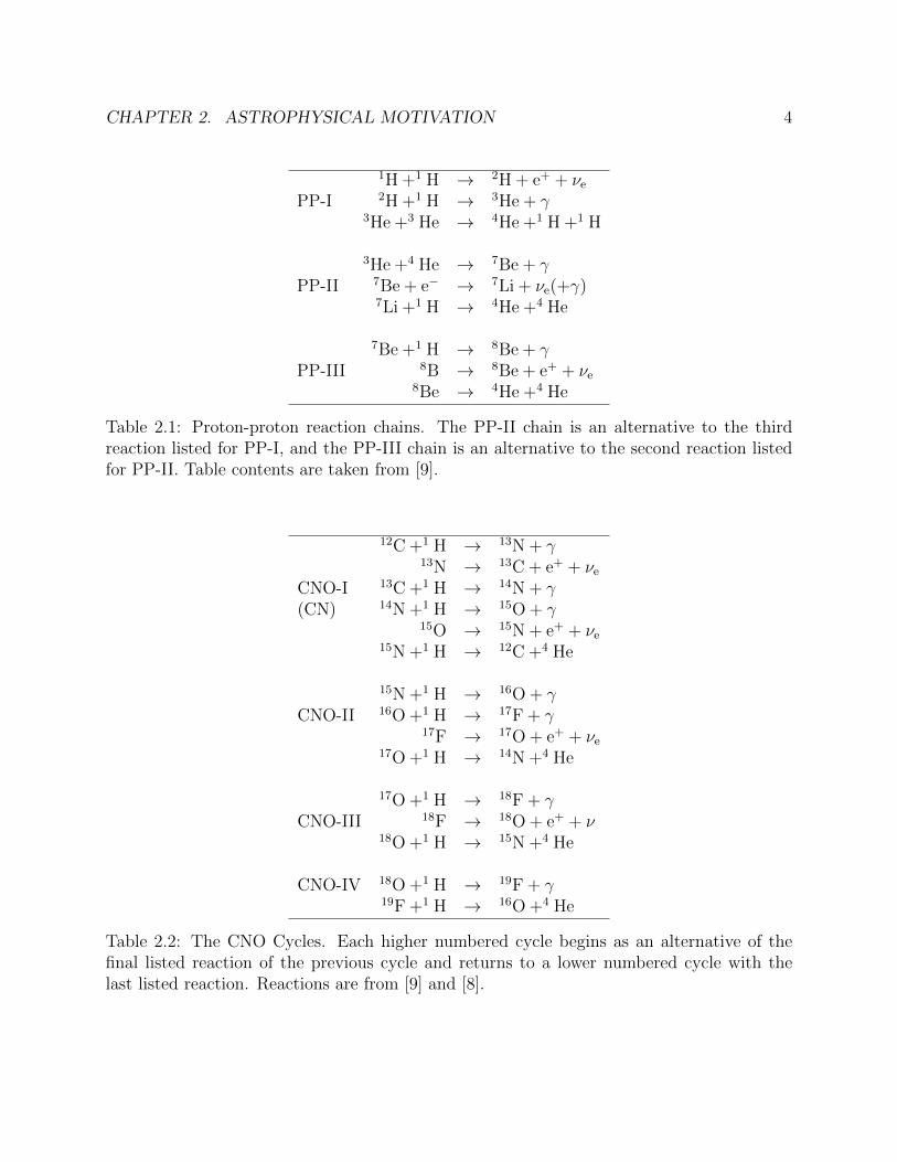
The evolution of a star is a sequence of gravitational contraction and nuclear reactionphases[8]. When a cloud of gas contracts the gravitational potential energy released providesa source of thermal energy which allows the ignition of the first nuclear burning phase,hydrogen burning. Hydrogen burning can follow the p-p chain, one of the CNO cycles (I-IV,or at higher temperatures the “Hot CNO” cycle), the NeNa cycle, or the MgAl cycle. Thep-p chain reactions are listed in Table 2.1 and the CNO cycle reactions are listed in Table2.2. Which reaction is dominant depends on the temperature of the star. The sun generatesabout 10% of its energy from the CNO cycle, though at core temperatures slightly higherthan the sun the CNO cycle will dominate[9]. The CNO cycle also requires the presence ofcarbon, nitrogen, and oxygen catalysts that are not present in first generation stars, limitingthese stars to the proton-proton chains.
Hydrogen burning provides pressure in stars that prevents further gravitational contrac-tion. Since this is the longest burn phase, stars in their hydrogen burning phase are referredto as main sequence stars[8]. Higher mass stars have higher luminosity since more pressurefrom the burn is required to find equilibrium. As a result, higher mass stars exhaust theirhydrogen fuel in less time than lower mass stars. As the hydrogen fuel is exhausted, gravi-tational contraction again takes over until the temperatures needed for helium burning arereached. In the process, the gravitational contraction will accelerate the hydrogen burningnear the core, driving the outer layer away from the core to form a red giant[8].
Helium burning proceeds by the triple alpha process. This process can be thought ofas two reactions. The first is 4He +4 He↔8 Be. The isotope 8Be has a very short (10−16
seconds) lifetime and so to have a significant population of 8Be the temperature needs to
CHAPTER 2. ASTROPHYSICAL MOTIVATION 4
1H +1 H → 2H + e+ + νe
PP-I 2H +1 H → 3He + γ3He +3 He → 4He +1 H +1 H
3He +4 He → 7Be + γPP-II 7Be + e− → 7Li + νe(+γ)
7Li +1 H → 4He +4 He
7Be +1 H → 8Be + γPP-III 8B → 8Be + e+ + νe
8Be → 4He +4 He
Table 2.1: Proton-proton reaction chains. The PP-II chain is an alternative to the thirdreaction listed for PP-I, and the PP-III chain is an alternative to the second reaction listedfor PP-II. Table contents are taken from [9].
12C +1 H → 13N + γ13N → 13C + e+ + νe
CNO-I 13C +1 H → 14N + γ(CN) 14N +1 H → 15O + γ
15O → 15N + e+ + νe15N +1 H → 12C +4 He
15N +1 H → 16O + γCNO-II 16O +1 H → 17F + γ
17F → 17O + e+ + νe17O +1 H → 14N +4 He
17O +1 H → 18F + γCNO-III 18F → 18O + e+ + ν
18O +1 H → 15N +4 He
CNO-IV 18O +1 H → 19F + γ19F +1 H → 16O +4 He
Table 2.2: The CNO Cycles. Each higher numbered cycle begins as an alternative of thefinal listed reaction of the previous cycle and returns to a lower numbered cycle with thelast listed reaction. Reactions are from [9] and [8].
CHAPTER 2. ASTROPHYSICAL MOTIVATION 5
reach a minimum of about 1.2 ∗ 108 Kelvin[9] where a significant population of 4He canaccess the resonant reaction to the ground state of 8Be. With a population of 8Be formedthe capture reaction 8Be +4 He↔12 C can proceed. The carbon is formed in its 7.654 MeVexcited state which has a high probability of emitting an alpha, so again a high productionrate of the excited 12C is needed so that the gamma decay channel can produce significantquantities of ground state 12C[9].
Following helium burning, gravitational contraction can continue to begin carbon burn-ing. In this process, two carbon nuclei are consumed, producing neon, sodium, or magnesium.The amount of each product is determined by the branching ratio of the nuclear reaction aswell as by the total reaction rate. At stellar temperatures the total reaction rate is dominatedby the Coulomb barrier[8][9]. Since the average kinetic energy of the carbon nuclei is wellbelow the Coulomb barrier, the total cross section is very small, and rapidly decreases withdecreasing energy. Attempts to measure the cross section using particle accelerators becomesincreasingly difficult as the energy is decreased closer to those of astrophysical interest.
The Coulomb barrier is not as restrictive to the exit channels. The alpha and protonchannels which produce neon and sodium are both exothermic [10] and release enough energythat even if the two carbon nuclei had zero kinetic energy, the alpha particle or proton wouldbe above its Coulomb barrier. The neutron channel has no Coulomb barrier, but is slightlyendothermic and only contributes at higher energies. In principle two carbon nuclei couldalso be emitted, however the same Coulomb barrier which dominates the total reaction ratemakes this channel very small.
While any measurement of the entrance channel will have to contend with the 12C +12 CCoulomb barrier in some manner, measuring the exit channels alone can avoid this difficulty.By recreating the nuclear conditions which occur after two carbon nuclei penetrate theirmutual Coulomb barrier, the exit channels’ branching ratios can be measured. By makingsome assumptions about the compound nucleus, primarily that the particles come to thermalequilibrium prior to particle emission, this becomes a realistic approach [11].
2.2 The Gamow Window
The nuclei within a star have a thermal distribution given by the Maxwell-Boltzmannvelocity distribution
φ(v) = 4πv2( m
2πkT
)3/2
exp
(−mv
2
2kT
)(2.1)
or in terms of energy as[8]
φ(E) ∝ E ∗ exp(−E/kT ) (2.2)
At high energies (E � kT ) the density decreases exponentially with increasing energy.
CHAPTER 2. ASTROPHYSICAL MOTIVATION 6
The nuclear reaction cross sections for charged particles at stellar energies are dominatedby the probability of penetrating the Coulomb barrier. At energies well below the Coulombbarrier peak this penetration probability is approximated by
P = exp(−2πη) (2.3)
where η is the Sommerfeld parameter η = Z1Z2e2
hv= 31.29
2πZ1Z2
(µE
)1/2[8]. It is common to
express astrophysical cross sections in the form
σ(E) =1
Eexp(−2πη)S(E) (2.4)
where the 1E
term accounts for the energy dependence of the de Broglie wavelength (πλ2 ∝ 1E
)which relates to the classical analog of the area of the target as seen by the projectile, andthe term S(E) contains the nuclear effects on the cross section. In the absence of resonancesS(E) is a slowly changing function of energy[8].
The reaction rate is a function of both the cross section at a given energy and the popu-lation of the reacting nuclei at that energy. Thus for a given temperature the (differential)reaction rate as a function of energy is of the form
dr
dE∝ φ(E)σ(E) (2.5)
where drdE
is the reaction rate at a given energy [8]. Entering the formulas for φ(E) and σ(E)from above results in
dr
dE∝ E ∗ exp(−E/kT )
1
Eexp(−2πη)S(E) = exp(−E/kT − 2πη)S(E) (2.6)
The energy dependence of 2πη can be separated out,
2πη =b
E1/2(2.7)
where b = (2µ)1/2πe2Z1Z2/h = 0.989Z1Z2µ1/2(MeV )1/2. This defines the Gamow energy,
which is b2 [8].Assuming that S(E) is relatively constant, the reaction rate as a function of energy can
be qualitatively described by
dr
dE∝ exp
(− E
kT− b
E1/2
)(2.8)
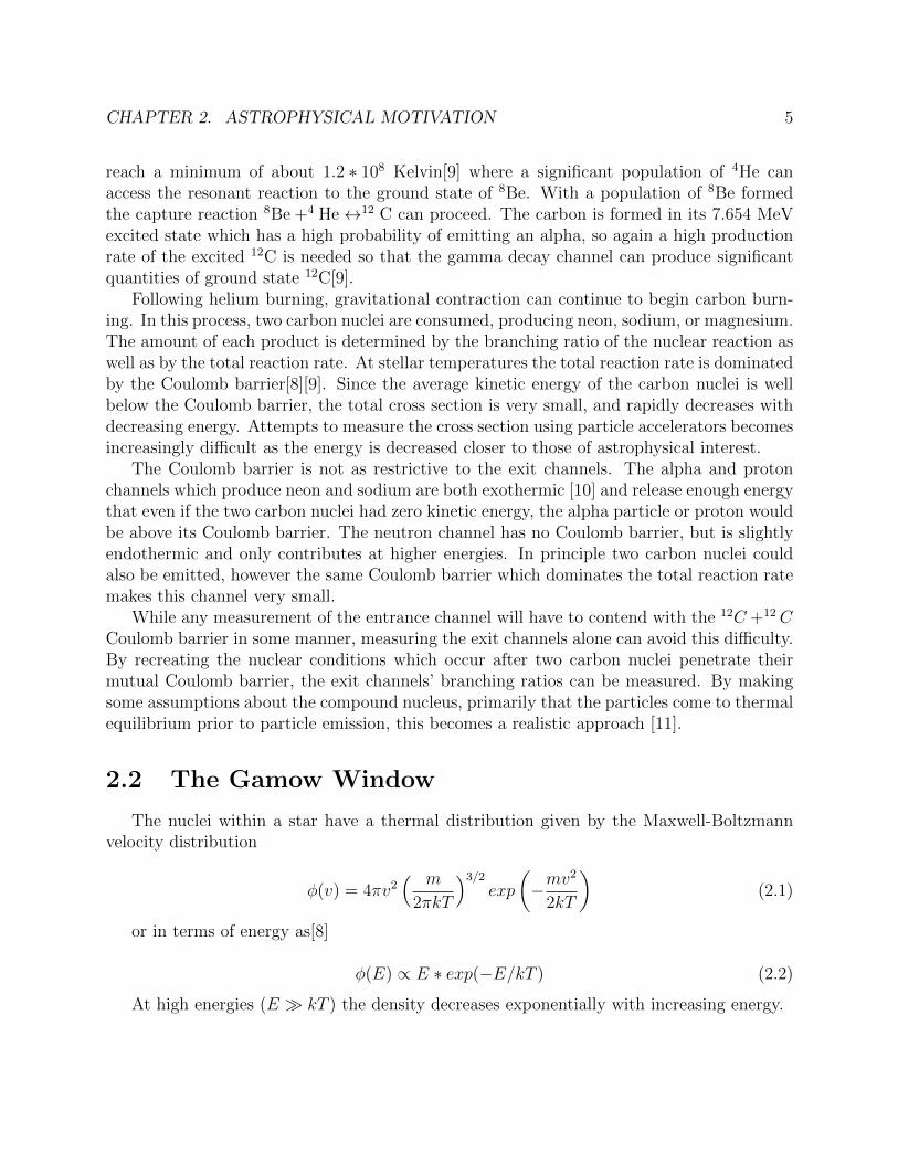
This is shown in Figure 2.1.A feature of this function is a peak where most reactions occur. The energy range
containing this peak is the Gamow window. At energies above the Gamow window thethermal population of nuclei is too small to have a significant contribution to the total
CHAPTER 2. ASTROPHYSICAL MOTIVATION 7
0.5 1 1.5 2 2.5
Arb
itra
ryU
nit
s
MeV
Gamow Peak
Gamow PeakThermal Distribution
Coulomb Barrier Penetration
Figure 2.1: An approximation of the reaction rate as a function of energy for two 12C nucleiat 5 ∗ 108 Kelvin. The units for the vertical axis are arbitrary. This is similar to a plot in[8].
CHAPTER 2. ASTROPHYSICAL MOTIVATION 8
reaction rate, and at energies below the Gamow window the cross section falls off too rapidlyto have a significant contribution. As a result, cross section measurements are most usefuland will have the greatest impact in the energy range of the Gamow window.
2.3 Steady Carbon Burning
In stars of greater mass than around 8-10 times that of the sun carbon burning can occurat a steady rate following the hydrogen and helium burning phases. For example a 25 solarmass star will undergo a steady carbon burning phase for around 600 years[8]. This processoccurs at a temperature around 5 ∗ 108 K [8].
2.4 Supernovae
A bright nova was identified with the combination of the observation the nova on Au-gust 31, 1885 by Hartwig in the Andromeda galaxy and the estimation of the distance toAndromeda galaxy by Lundmark in 1920[12] [13]. The distinction between novae and super-novae was first made by Baade and Zwicky in 1934 [14] [13]. Initially the distinction betweennovae and supernovae was one of magnitude, with supernovae releasing on the order of 1000times the energy of other novae. Novae are the result of mass transfer in a binary starsystem, eventually causing the transferred hydrogen to ignite, leading to a greatly increasedbrightness which fades over time. The two binary stars remain and the cycle can repeat[9]. Some but not all types of supernovae involve binary systems and the explosion in asupernova leads to a major change in the star itself, such as complete disruption, a remnantwhite dwarf, neutron star, or black hole [9]. The division of supernovae into types I and IIwas made in 1940 by Minkowski [15]. A further division of type I supernovae was made byWheeler and Harkness [16] after studies going back as early as 1960 [17] [18] [19].
Type Ia supernovae have become of particular interest due to their use as distance indi-cators or standard candles. The idea that supernovae could be used to estimate distancesto galaxies was proposed by both Zwicky in 1938 [20] and Wilson in 1939 [21] due to theirrelatively uniform brightness. Most of the supernovae which led to this conclusion were laterdetermined to be of type Ia [13].
While type Ia supernovae do appear fairly uniform, they do exhibit enough variabilitythat there may be differences among the source stars and the explosion mechanisms [13].This leads to a desire for a well understood explosion model, hopefully leading to a greaterconfidence when using these supernovae to estimate distances.
Numerous models have been proposed for explaining in paticular type Ia supernovae.These models can be divided into Chandrasekhar mass explosion models, sub- chandrasekharmass models and colliding white dwarf models. Chadrasekhar mass models can further bedivided into deflagration, delayed detonation and pulsed detonation models [13] which differ
CHAPTER 2. ASTROPHYSICAL MOTIVATION 9
in the manner in which the reaction front travels through the star.Chandrasekhar mass explosion models are based on a white dwarf star gaining material
from a nearby companion star until it approaches the Chandrasekhar mass, the mass whichcan be supported by electron degeneracy. Such a star then begins to contract, convertinggravitational energy into heat and igniting the primarily carbon fuel to create a supernova[17].
Soon after the distinction between novae and supernovae was made by Baade and Zwickyit was also recognized that supernovae were good candidates for producing heavy elements.An early model for this was that a statistical equilibrium would form in supernovae betweenradiation and radioactive nuclei [22]. For a density of 107 grams/cm and a temperature of4 ∗ 109 kelvin this equilibrum is reached in about 100 seconds, with a strong dependence ontemperature [22].
2.5 Previous Measurements
A number of direct measurements have been made by bombarding a 12C target with a12C beam [1] [2] [3] [4] [5] [6] [7]. Many of these experiments measured the alpha, protonand neutron channels by detecting the emitted gamma rays from the resulting 20Ne, 23Naand 23Mg nuclei [2] [4] [5] [6] [7]. This method only measures the reactions which producean excited product nuclei. The portion of the reaction producing ground state nuclei mustbe added in by theory or by comparison to other experiments.
Some differences exist in the various data sets. The total fusion cross section differencesare discussed and a potential resolution is presented by Aguilera et al. [5] who proposed ashift in the energy scale and a normalization factor be applied to each data set. These factorswere justified by the possibility that carbon could build up on a target and compromise theenergy measurement of outgoing particles as well as the measurement of the total numberof target atoms. Since the total cross section is rapidly decreasing with decreasing energy,a small shift in the energy scale can result in a large change in the measured cross section.In the vicinity of 4.5 MeV, a 200 keV shift results in approximately a factor of 2 change intotal cross section [5].
A few methods have been proposed to extend the total cross section measurements tolower energies. One method uses the generalized optical theorem [23] [24] to relate thetotal reaction cross section to the angular elastic scattering cross section [25]. This methodrequires good angular resolution and statistics, particularly at small forward angles. Othermethods rely on theoretical models such as that by Jiang, Rehm, Back, and Janssens[26].The theoretical models can differ by up to two orders of magnitude for a kinetic energy of 1.5MeV [8]. This is partly due to the influence of resonances at these energies, and the variationsin the available cross section datasets mentioned above, especially at energies below about3 MeV [26]. Some datasets, notably that of Mazarakis and Stephens [1] fall off less thanwould be expected for the Coulomb barrier. This would be consistent with the phenomenon
CHAPTER 2. ASTROPHYSICAL MOTIVATION 10
of “absorption under the barrier” which allows some fusion to initiate at distances greaterthan the nuclear radius. Other datasets such as that of Becker et al. [3] do not appear tohave this feature, which seems to give evidence against absorption under the barrier. Theexistence or absence of absorption under the barrier should not affect the branching ratioshowever.
2.6 Branching Ratios
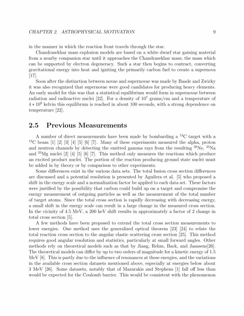
The 12C +12 C reaction can proceed through several channels. The primary two channelswhich are energetically possible at any 12C +12 C energy are 12C(12C, α)20Ne and12C(12C, p)23Na. At higher energies the reaction 12C(12C, n)23Mg also becomes important.Other possible reactions, such as those leaving an oxygen nucleus as a product, are notfavored at low energies due to the large Coulomb barrier present in these exit channels.
The relative probability of each exit channel is referred to as the “branching ratio” ofthat channel. The branching ratio is defined by the ratio of the cross section of the reactionleading to a specific exit channel to the sum of all cross sections of reactions leading to anyexit channel. As a result, the sum of the branching ratios of all of the exit channels is one.In the present context, the branching ratio gives the probability that a specific nuclei suchas 20Ne is produced given that two 12C nuclei fuse into a compound nucleus.
Branching Ratio =σchannelσsum
(2.9)
CHAPTER 2. ASTROPHYSICAL MOTIVATION 11
Gamow
Q (MeV) =
12C +12 C0.0
-14.0
@@
-4.0
-3.0
-2.0
-1.0
1.0
2.0
3.0
4.0MeV, CM MeV
24Mg13.934
0.0
@@
10.0
11.0
12.0
13.0
14.0
15.0
16.0
17.0
@@ @@
20Ne+ α4.617
23Na+ p2.241
23Mg + n-2.598
Figure 2.2: Level Diagram for the isotopes of interest. The approximate location of theGamow window is shown by the horizontal band.
CHAPTER 2. ASTROPHYSICAL MOTIVATION 12
Reaction Q Value Coulomb Barrier Difference(Exit Channel)
(NNDC [10]) (Bass [27][28])12C +12 C 5.413 MeV
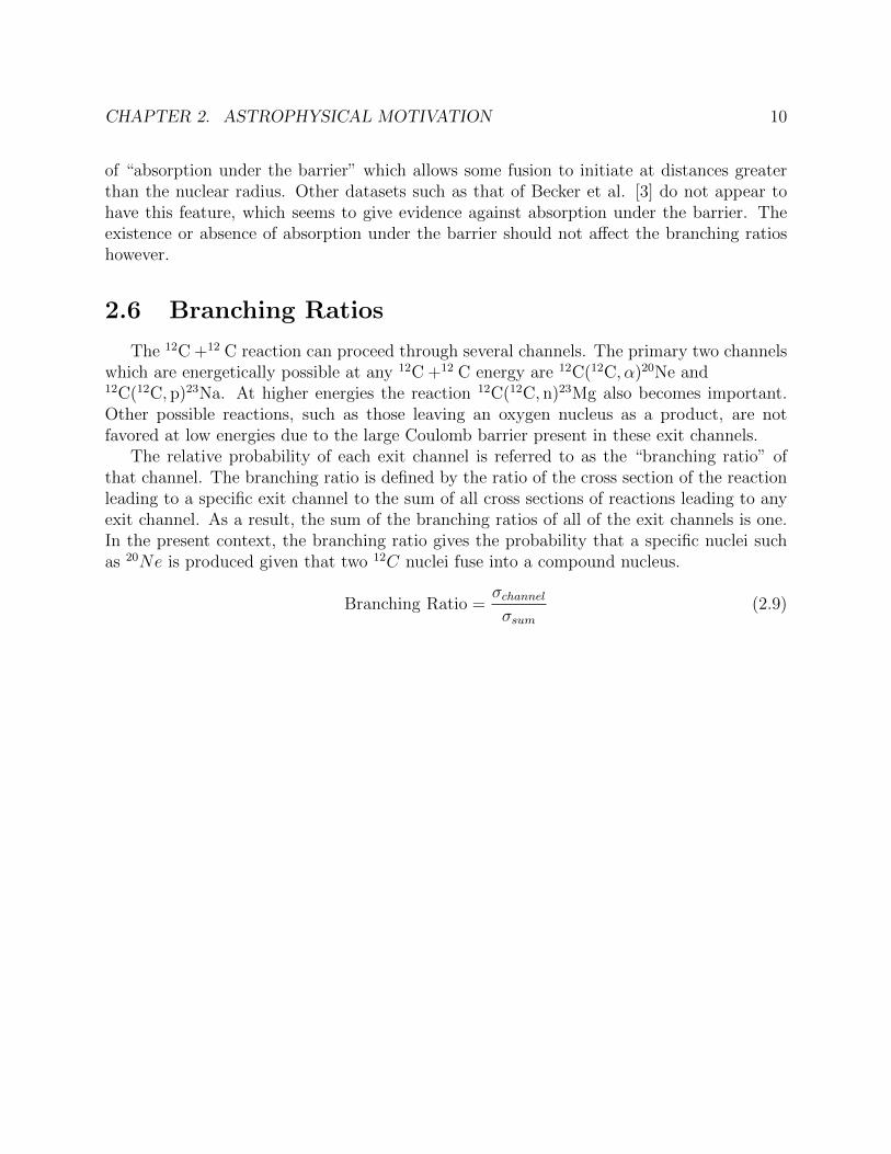
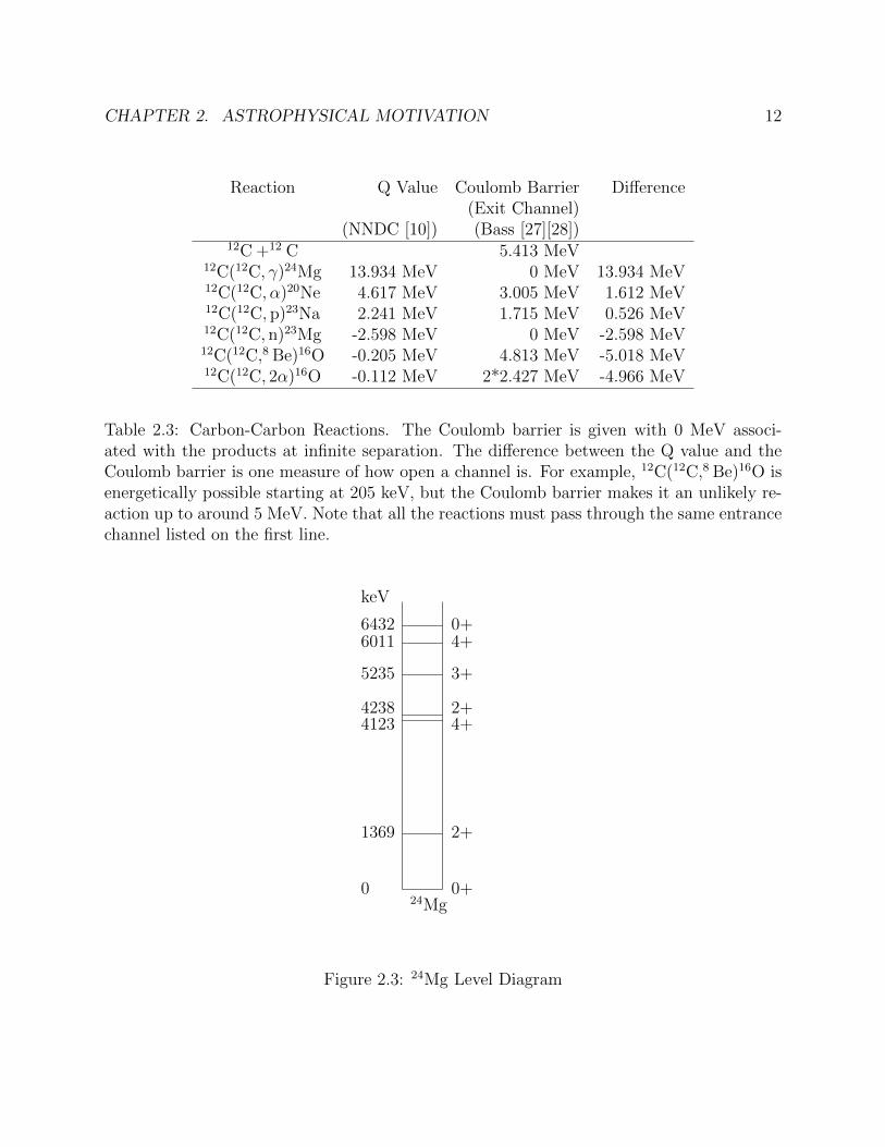
12C(12C, γ)24Mg 13.934 MeV 0 MeV 13.934 MeV12C(12C, α)20Ne 4.617 MeV 3.005 MeV 1.612 MeV12C(12C, p)23Na 2.241 MeV 1.715 MeV 0.526 MeV12C(12C, n)23Mg -2.598 MeV 0 MeV -2.598 MeV12C(12C,8 Be)16O -0.205 MeV 4.813 MeV -5.018 MeV12C(12C, 2α)16O -0.112 MeV 2*2.427 MeV -4.966 MeV
Table 2.3: Carbon-Carbon Reactions. The Coulomb barrier is given with 0 MeV associ-ated with the products at infinite separation. The difference between the Q value and theCoulomb barrier is one measure of how open a channel is. For example, 12C(12C,8 Be)16O isenergetically possible starting at 205 keV, but the Coulomb barrier makes it an unlikely re-action up to around 5 MeV. Note that all the reactions must pass through the same entrancechannel listed on the first line.
keV
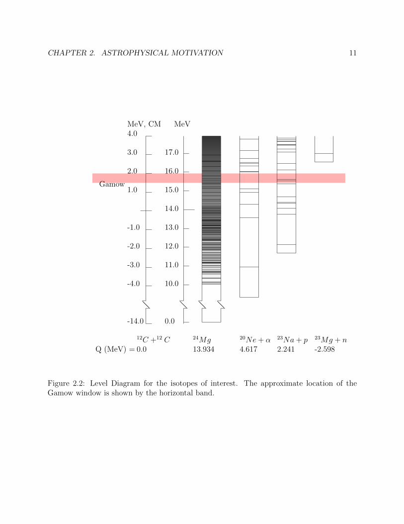
24Mg0 0+
1369 2+
4123 4+4238 2+
5235 3+
6011 4+6432 0+
Figure 2.3: 24Mg Level Diagram
CHAPTER 2. ASTROPHYSICAL MOTIVATION 13
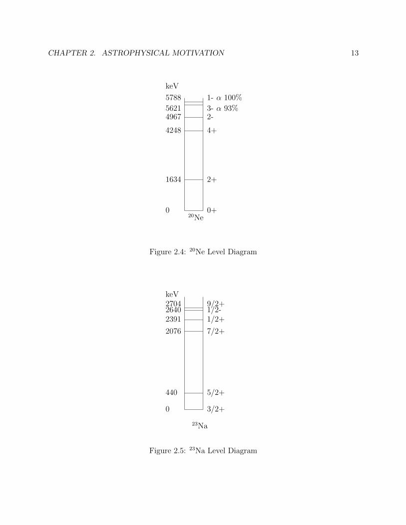
keV
20Ne0 0+
1634 2+
4248 4+
4967 2-5621 3- α 93%
5788 1- α 100%
Figure 2.4: 20Ne Level Diagram
keV
23Na
0 3/2+
440 5/2+
2076 7/2+
2391 1/2+2640 1/2-2704 9/2+
Figure 2.5: 23Na Level Diagram
CHAPTER 2. ASTROPHYSICAL MOTIVATION 14
An idea of which exit channels are important can be developed by looking at the Coulombbarriers and Q values for each reaction. These are shown in Table 2.3 and a level diagramfor the A = 24 system is shown in Figure2.2. If the Q value plus the initial kinetic energyis less than the Coulomb barrier then the emitted particle would have to tunnel throughthe Coulomb barrier. This would make the exit channel much less favorable and greatlydiminish its branching ratio. If the Q value plus the initial kinetic energy is negative, thenthe exit channel is not energetically possible. Additionally, since nuclear forces are muchstronger than electromagnetic forces, channels which emit particles will be favored to thosewhich emit gamma rays when there is sufficient energy for the emitted particles to clear theCoulomb barrier. This is why 24Mg is not a major exit channel for the 12C +12 C reactiondespite the high Q value and the absence of a Coulomb barrier for the gamma ray.
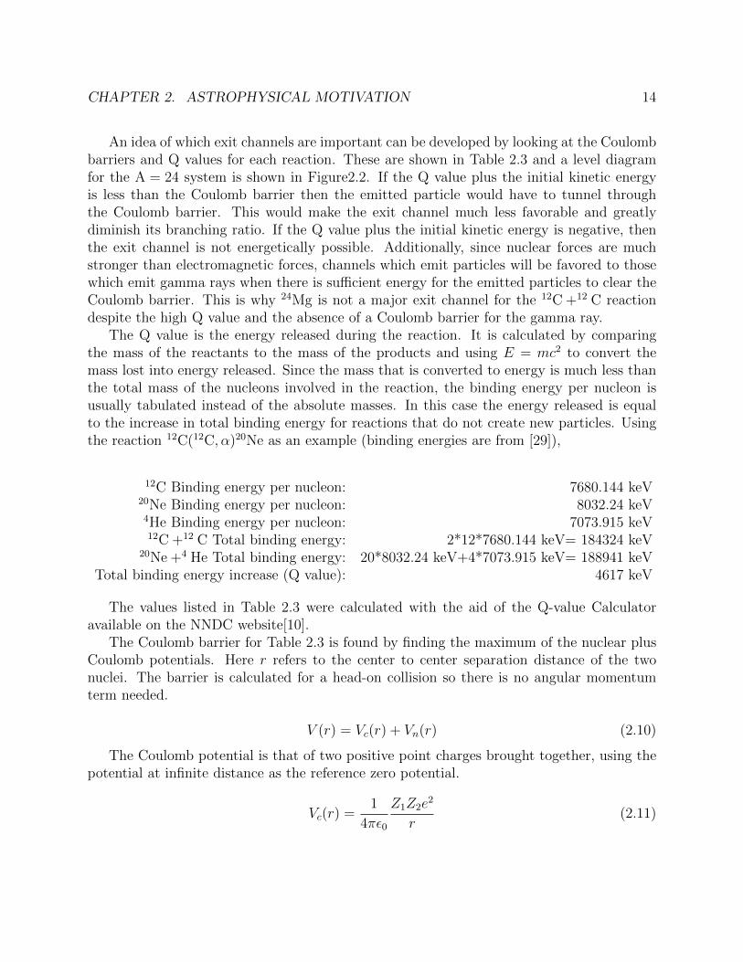
The Q value is the energy released during the reaction. It is calculated by comparingthe mass of the reactants to the mass of the products and using E = mc2 to convert themass lost into energy released. Since the mass that is converted to energy is much less thanthe total mass of the nucleons involved in the reaction, the binding energy per nucleon isusually tabulated instead of the absolute masses. In this case the energy released is equalto the increase in total binding energy for reactions that do not create new particles. Usingthe reaction 12C(12C, α)20Ne as an example (binding energies are from [29]),
12C Binding energy per nucleon: 7680.144 keV20Ne Binding energy per nucleon: 8032.24 keV4He Binding energy per nucleon: 7073.915 keV12C +12 C Total binding energy: 2*12*7680.144 keV= 184324 keV
20Ne +4 He Total binding energy: 20*8032.24 keV+4*7073.915 keV= 188941 keVTotal binding energy increase (Q value): 4617 keV
The values listed in Table 2.3 were calculated with the aid of the Q-value Calculatoravailable on the NNDC website[10].
The Coulomb barrier for Table 2.3 is found by finding the maximum of the nuclear plusCoulomb potentials. Here r refers to the center to center separation distance of the twonuclei. The barrier is calculated for a head-on collision so there is no angular momentumterm needed.
V (r) = Vc(r) + Vn(r) (2.10)
The Coulomb potential is that of two positive point charges brought together, using thepotential at infinite distance as the reference zero potential.
Vc(r) =1
4πε0
Z1Z2e2
r(2.11)
CHAPTER 2. ASTROPHYSICAL MOTIVATION 15
-4
-2
0
2
4
6
8
10
4 6 8 10 12 14 16 18 20
MeV
Center to Center Distance (fm)
Coulomb Barrier
Barrier Height
Coulomb PotentialNuclear Potential
Total Potential
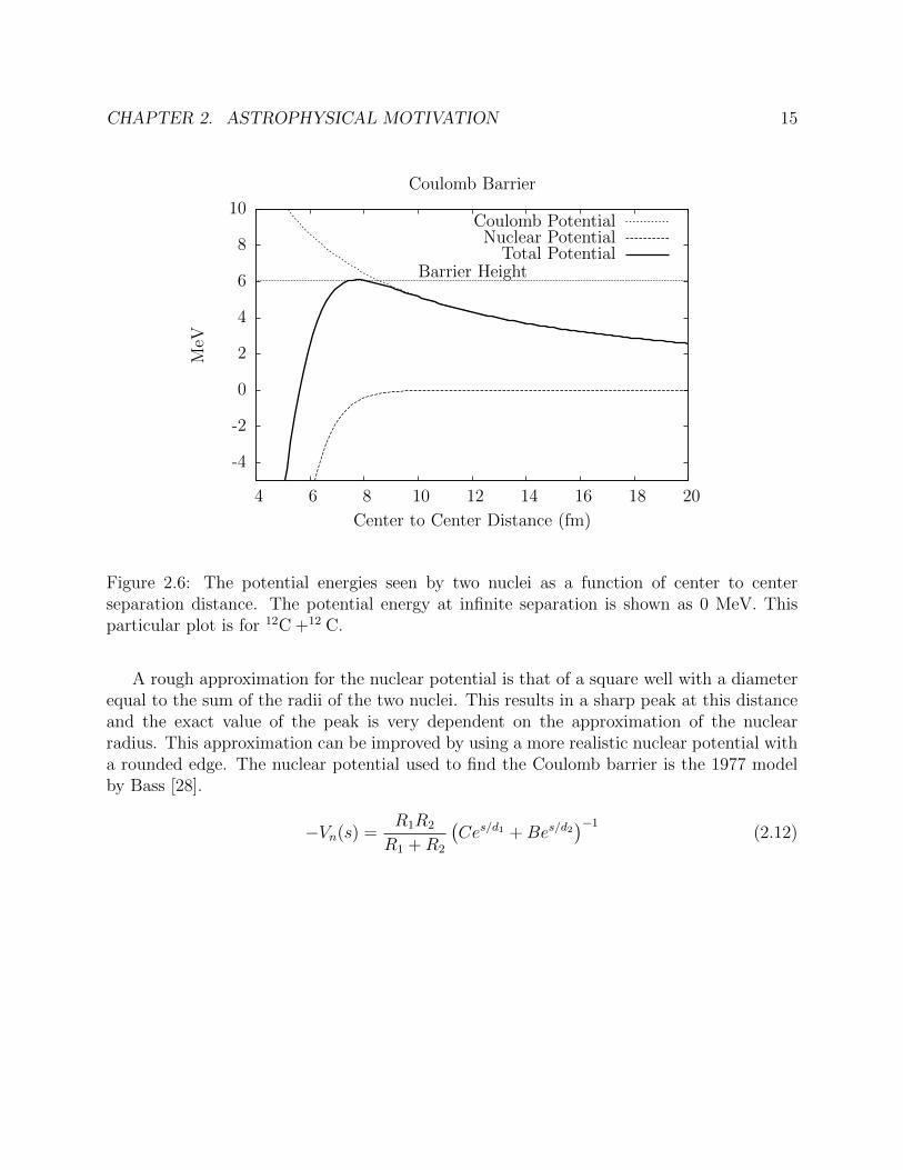
Figure 2.6: The potential energies seen by two nuclei as a function of center to centerseparation distance. The potential energy at infinite separation is shown as 0 MeV. Thisparticular plot is for 12C +12 C.
A rough approximation for the nuclear potential is that of a square well with a diameterequal to the sum of the radii of the two nuclei. This results in a sharp peak at this distanceand the exact value of the peak is very dependent on the approximation of the nuclearradius. This approximation can be improved by using a more realistic nuclear potential witha rounded edge. The nuclear potential used to find the Coulomb barrier is the 1977 modelby Bass [28].
−Vn(s) =R1R2
R1 +R2
(Ces/d1 +Bes/d2
)−1(2.12)
CHAPTER 2. ASTROPHYSICAL MOTIVATION 16
where
r =Center to Center distance
C =0.0300 fm/MeV
B =0.0061 fm/MeV
d1 =3.30 fm
d2 =0.65 fm
s =r −R1 −R2 = Surface separation distance
and
R =aA1/3 − b2(aA1/3)−1 = the nuclear radius
a =1.16 fm
b2/a =1.39 fm
A =the atomic mass of the nucleus.
Finally, equations 2.11 and 2.12 are inserted into equation 2.10. The peak location isfound where the derivative with respect to the separation distance (or equivalently the centerto center distance since this is offset by a constant) is zero, and evaluating the potential atthis location gives the height of the Coulomb barrier. A graphical representation of thepotential energies is shown in Figure 2.6.
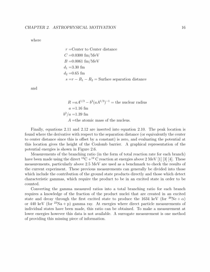
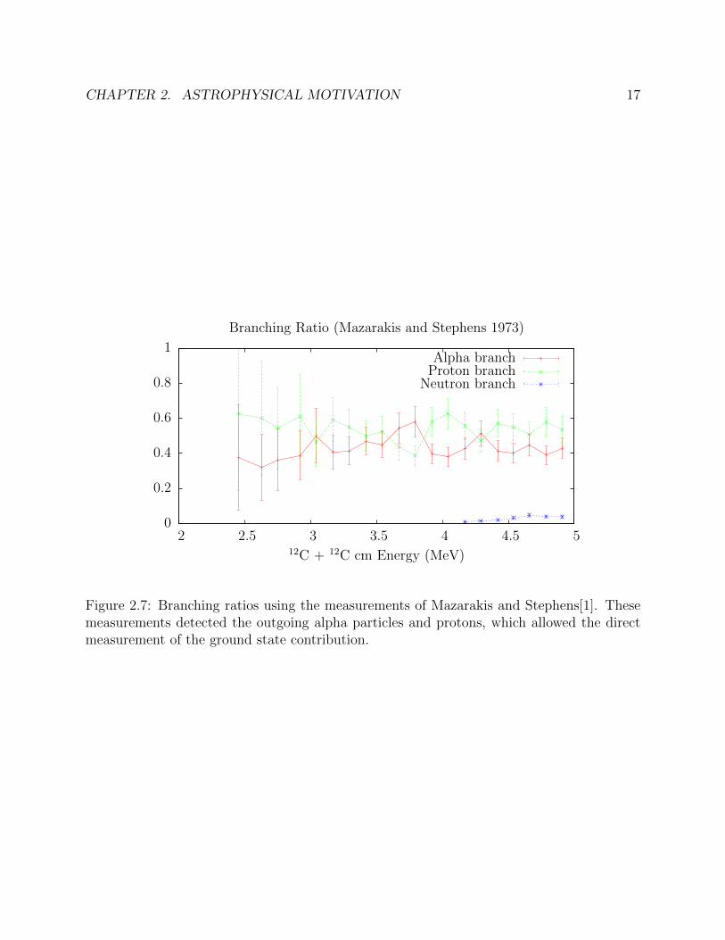
Measurements of the branching ratio (in the form of total reaction rate for each branch)have been made using the direct 12C +12 C reaction at energies above 2 MeV [1] [3] [4]. Thesemeasurements, particularly above 2.5 MeV are used as a benchmark to check the results ofthe current experiment. These previous measurements can generally be divided into thosewhich include the contribution of the ground state products directly and those which detectcharacteristic gammas, which require the product to be in an excited state in order to becounted.
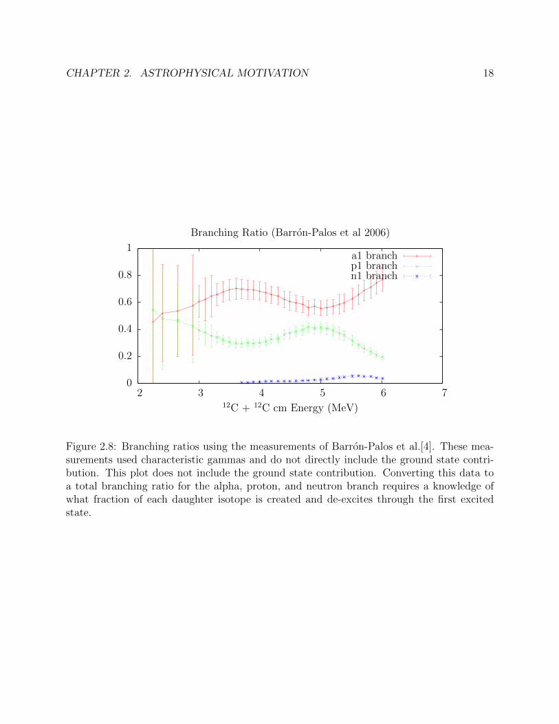
Converting the gamma measured ratios into a total branching ratio for each branchrequires a knowledge of the fraction of the product nuclei that are created in an excitedstate and decay through the first excited state to produce the 1634 keV (for 20Ne + α)or 440 keV (for 23Na + p) gamma ray. At energies where direct particle measurements ofindividual states have been made, this ratio can be obtained. To make a measurement atlower energies however this data is not available. A surrogate measurement is one methodof providing this missing piece of information.
CHAPTER 2. ASTROPHYSICAL MOTIVATION 17
0
0.2
0.4
0.6
0.8
1
2 2.5 3 3.5 4 4.5 512C + 12C cm Energy (MeV)
Branching Ratio (Mazarakis and Stephens 1973)
Alpha branchProton branch
Neutron branch
Figure 2.7: Branching ratios using the measurements of Mazarakis and Stephens[1]. Thesemeasurements detected the outgoing alpha particles and protons, which allowed the directmeasurement of the ground state contribution.
CHAPTER 2. ASTROPHYSICAL MOTIVATION 18
0
0.2
0.4
0.6
0.8
1
2 3 4 5 6 712C + 12C cm Energy (MeV)
Branching Ratio (Barron-Palos et al 2006)
a1 branchp1 branchn1 branch
Figure 2.8: Branching ratios using the measurements of Barron-Palos et al.[4]. These mea-surements used characteristic gammas and do not directly include the ground state contri-bution. This plot does not include the ground state contribution. Converting this data toa total branching ratio for the alpha, proton, and neutron branch requires a knowledge ofwhat fraction of each daughter isotope is created and de-excites through the first excitedstate.
19
Chapter 3
Surrogate Method
Many cross sections are difficult to measure directly for various reasons. The surrogatemethod has been used to measure fission and other cross sections for a number of heavynuclei by the STARS/LiBerACE [11], STARLiTe, and STARLiTeR groups. For a numberof these experiments, direct (n, f) measurements were impractical due to the short half lifeof the target nuclei, requiring other reactions on neighboring nuclei (“surrogate reactions”)to be measured in order to infer the desired (n, f) cross section.
The surrogate method relies on the existence of an intermediate state called the compoundnucleus which is a mixture of the beam and target particles’ nucleons. The energy of theparticles is in thermodynamic equilibrium and individual particles are not identified by theirorigin in the target nucleus or the beam nucleus. This hypothesis allows the conclusion thatthe same compound nucleus can be produced for study using a number of beam and targetpairings[11]. The key items to match in the compound nucleus are the number of protonsand neutrons, the excitation energy, and spin distribution. The best entrance channel touse is a compromise between getting the closest matching compound nucleus and choosingbeam and target nuclei which are experimentally feasible to work with.
In the case of 12C +12 C reactions, the compound nucleus is 24Mg. The Q value going tothe compound nucleus is just under 14 MeV. Since the stellar reactions of interest occur atenergies around 1.5 MeV, a typical excitation energy of interest in the compound nucleus isaround 15.5 MeV. A formation reaction that produces 24Mg in a range of excitations betweenabout 14 and 20 MeV is desired.
To further improve the measurement, angular momentum should be considered. Angularmomentum comes into the compound nucleus in two ways. One is from the intrinsic spinof the colliding particles. The 12C nucleus has an intrinsic angular momentum of 0, makingthis contribution 0 for 12C +12 C reactions. The other contribution comes from the orbitalangular momentum of the impact. A convenient image for this contribution is two ballshitting each other either head on or receiving a glancing blow, then being glued together onimpact. The head on case delivers no angular momentum, while the glancing blow wouldprovide the maximum angular momentum. Using this model and typical estimates for the
CHAPTER 3. SURROGATE METHOD 20
radii of a 12C nucleus leads to spins up to 3h to 4h.The difference in the reaction rates as a result of this potential spin difference can be
neglected if certain criteria are met [30]. A primary condition is that the excitation energymust be sufficiently high that the possible branches are dominated by level density integralsrather than individual states [31]. This independence of the branching ratios from spin andparity is called the Weisskopf-Ewing approximation. For carbon burning reactions this ismet for the compound nucleus but not for the daughter nuclei, therefore matching the spindistribution for the compound nucleus is still important to minimize the change in branchingratios that may occur due to different spin distributions.
Several reactions can be considered. The first is the direct method using 12C +12 C.This method requires very high beam currents at low energies due to the Coulomb barrier.Measurements using this method are discussed in Chapter 2 Section 2.5. Similarly, otherreactions with two larger atoms such as 14N +10 B would generally see similar Coulombbarriers and not escape the fundamental difficulty with 12C +12 C.
The reactions 20Ne + α and 23Na + p both bring in smaller amounts of angular momen-tum from the collision (though the sodium reaction has intrinsic momentum it brings in)and do not have prohibitive Coulomb barriers. However, to scan different amounts of excita-tion in the compound nucleus using these reactions would require many runs using differentbeam energies. Also, the channels to be measured would often have the same signature inthe detector as scattering reactions. For example if the compound nucleus was populatedwith the reaction 20Ne + α and the outgoing alpha channel was measured, the result is ascattering measurement. Separation of the compound component and other components tothe scattering cross section (ie, elastic, direct inelastic, or pre-equilibrium inelastic) makesthis approach not ideal.
The approach that was selected is to excite 24Mg using inelastic scattering. Using inelasticexcitation allows for the scattered particle to be used to identify the excitation produced inthe surrogate compound nucleus1. By identifying the excitation of the compound nucleuson a per event basis the correct excitation distribution can be reconstructed for a range ofdifferent stellar temperatures.
Lighter ions are preferred for the inelastic excitation for a few reasons. First is thatlighter ions will provide a much clearer signature in a deltaE-E silicon detector setup afterscattering. Second, lighter ions will produce less angular momentum during collision. Dueto the beam needing a much higher energy than the kinetic energy of the 12C +12 C reaction,a tendency towards higher angular momenta needs to be counteracted. Using Talys[32]calculations, protons will produce angular momenta greater than 4 around 15% of the timeat 30 MeV while alpha particles will produce angular momenta greater than 4 around 35% to45% of the time. Therefore on reducing the higher spin population alone protons are slightly
1Since inelastic excitation does not combine two nuclei, referring to the resulting excited nucleus as acompound nucleus is not standard notation. The notation is kept here to emphasize the intended parallelbetween the excited 24Mg nucleus produced by inelastic excitation and the nucleus produced by combiningtwo 12C nuclei.
CHAPTER 3. SURROGATE METHOD 21
favorable, however alpha particles were ultimately selected because they would favorablypopulate the same parity pattern (0+, 2+, etc.) and because the scattered alpha particleshave a convenient stopping range in the silicon detector setup.
22
Chapter 4
Experimental Setup
4.1 Overview
Three experimental runs were performed. The first took place at the LBNL 88” Cyclotronstarting March 12, 2011 and ending the following day. This run was intended to be a testrun which would support a longer run if the results looked favorable. The second run wasat the TAMU K150 (88”) Cyclotron at the Texas A&M Cyclotron Institute and ran fromDecember 4, 2012 to December 12, 2012. Data from this run had problems with unexplainedlow energy particles being detected, and it was eventually decided that the measurementneeded to be repeated. The third and final run was also at the TAMU K150 Cyclotron andtook place from November 11, 2014 until November 18, 2014. Data from this final run atTAMU was used for the analysis.
The LBNL run made use of the STARS/LiBerACE [33] target chamber and detectorsystem. The Texas A&M runs made use of the STARLiTeR system, which is an upgrade ofthe STARS/LiBerACE system previously located at LBNL. The system includes the STARStarget chamber which holds the silicon detectors and target under vacuum and in line with theparticle beam, up to six germanium detectors each within a BGO detector whose purpose isto veto Compton scattering events in the germanium detector, and the electronics necessaryto record the signals from each detector. During operation, a master trigger is generatedwhich causes the readout for all detectors. For this experiment, the master trigger wasgenerated by a coincidence of the two downstream silicon detectors, described in Section 4.4.
4.2 Beam
An alpha particle beam with a nominal energy of 40 MeV was used for all three runs.During analysis, the beam energy was considered a free parameter which was fitted using theenergy of scattered beam at different angles for the various target masses (12C, 24Mg, and208Pb). The fitted values were close to the 40 MeV nominal value. The value adopted for
CHAPTER 4. EXPERIMENTAL SETUP 23
the final TAMU run was 39.58 MeV at the beginning of the run and 39.33 MeV at the end ofthe run. The change in the fitted value occurred over a period of about 24 hours during themiddle of the week long run. Fits within each stable period had a scatter of approximately0.07 MeV. The cause of the change was not positively identified.
The beam current was adjusted to be in the range of 1 to 1.5 nA for the first run andin the range of 0.5 to 2 nA for the second two runs when the primary 24Mg target wasin place. Trigger rates for the silicon detectors were the limiting factor for beam current.The final run at TAMU went though several periods when the beam current would oscillateby a factor of two or more. Efforts were made by the staff to smooth these oscillationswhen they occurred. These oscillations had the potential to affect the energy calibration ofthe detectors by causing the count rate to oscillate with the beam current and exceed thedesired maximum count rate, however this was not seen in the analysis and the data duringthese periods of current oscillation appears to be valid. The beam current for other targets(carbon, mylar, etc.) were adjusted such that the trigger rate was similar to that of the maintarget, which was typically around 7 to 10 kHz.
4.3 Targets
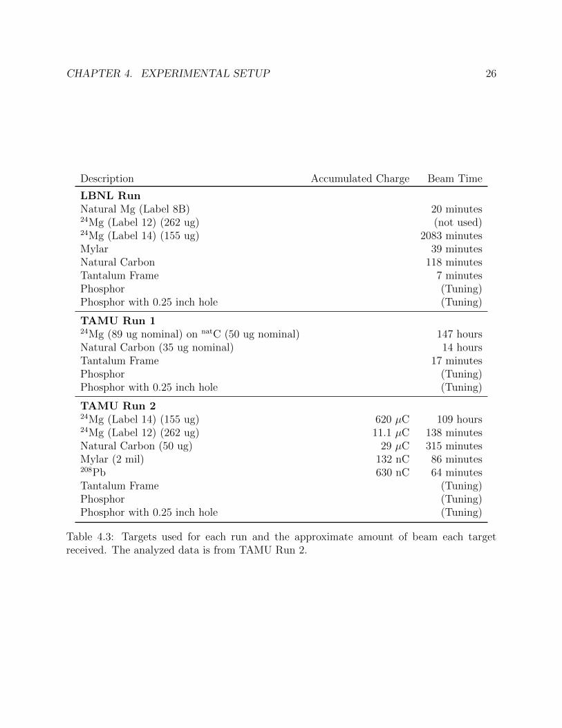
The STARS chamber[33] is designed to hold up to eight targets. A knob is locatedoutside the target chamber which can be manually turned in order to select which target isin the beam line. Each experiment had a different but similar array of targets which wereused during the experiment, including a primary 24Mg target, a carbon target for beamdiagnostics and carbon subtraction, and phosphors and an empty frame for tuning. Targetspresent for each run are listed in Table 4.3.
The LBNL test run and the second TAMU run both used a thin, self supporting 24Mgtarget as the primary target. Several self supporting magnesium targets were made priorto the LBNL run in an attempt to bring the thickness down as much as possible. Themagnesium used for the enriched targets was obtained from Oak Ridge National Laboratoryand was 99.9%± 0.02% 24Mg. Other isotopes and impurities in the original material arelisted in Table 4.1 and Table 4.2. These targets were made by using evaporation depositionof magnesium onto glass slides coated and buffed with Liquinox soap which was used as arelease agent, with the intent of removing the magnesium by “floating,” or slowly dippingthe glass slide at an angle into water, which would lift the magnesium and hold it on thesurface of the water with surface tension. This floating process is commonly used for carbonfoils. In practice the magnesium did not lift in this manner. The foils were instead removedby scraping a razor along the glass, creating a rolled tube of magnesium. This rolled tubewas unrolled by placing it on a piece of plastic which was then given a small electrostaticcharge using a cotton swab. Once the foil was unrolled, a glue-coated target frame was placeddirectly on top of the foil and slowly lifted. The main target was the thinnest target producedusing this method. Targets at this thickness were easy to tear during the scraping process and
CHAPTER 4. EXPERIMENTAL SETUP 24
Isotope Atomic Percent Precision24Mg 99.90 0.0225Mg 0.0726Mg 0.03
Table 4.1: Isotopic abundances for the enriched magnesium
all thinner attempts tore. The thinnest target successfully produced was used as the maintarget for both the LBNL run and the second TAMU run. The target thickness was measuredtwo ways. The first was using a second glass slide coated at the same time as the main target.This slide was measured to be 174 ug/cm2 at the center using a profilograph. The thicknesswas also measured using an alpha source and a silicon detector and relating the energy lostby the alpha to the thickness of the target. This measurement gave a thickness of 155± 10ug/cm2. Since this experiment is designed to measure ratios, the primary importance of thethickness measurement is to properly account for the energy lost by the particle within thetarget. Using a thin target minimizes this energy loss and the associated energy uncertainty.
The main target for the first TAMU run was made by coating a thin, mounted naturalcarbon backing with magnesium. The motivation for this was that the total target thicknesscould be lower than the thinnest freestanding magnesium target. Enriched 12C foils wereintended as the backing, but only foils from an older production run could be obtainedand these foils disintegrated during the floating process. The main target for this run was89 ug/cm2 on a carbon backing with a nominal thickness of 50 ug/cm2. The magnesiumthickness was measured using a glass plate coated at the same time as the carbon backingby a profilometer. During the experiment a natural carbon target from the same batch asthe carbon backing was used with the intent of subtracting the effects of the carbon backing.Difficulties with the data from the first TAMU run led to the decision to return to the olderfreestanding target for the second run, though it is not clear what role the carbon backingplayed in the data.
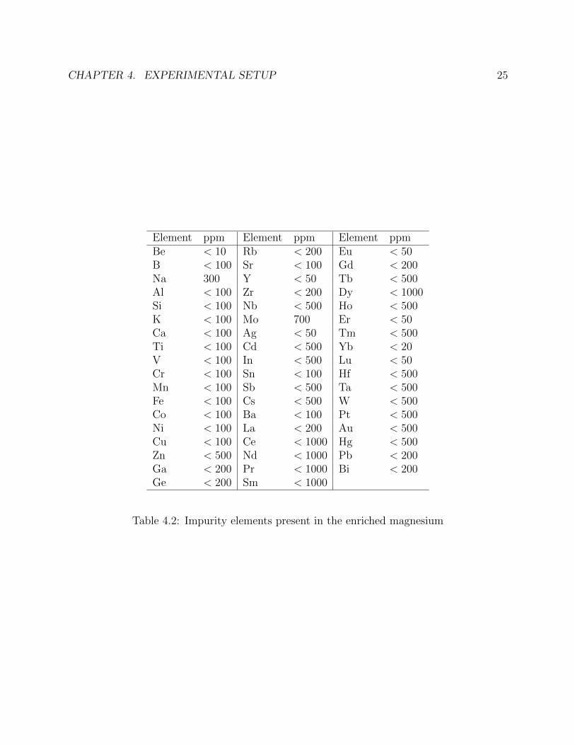
CHAPTER 4. EXPERIMENTAL SETUP 25
Element ppm Element ppm Element ppmBe < 10 Rb < 200 Eu < 50B < 100 Sr < 100 Gd < 200Na 300 Y < 50 Tb < 500Al < 100 Zr < 200 Dy < 1000Si < 100 Nb < 500 Ho < 500K < 100 Mo 700 Er < 50Ca < 100 Ag < 50 Tm < 500Ti < 100 Cd < 500 Yb < 20V < 100 In < 500 Lu < 50Cr < 100 Sn < 100 Hf < 500Mn < 100 Sb < 500 Ta < 500Fe < 100 Cs < 500 W < 500Co < 100 Ba < 100 Pt < 500Ni < 100 La < 200 Au < 500Cu < 100 Ce < 1000 Hg < 500Zn < 500 Nd < 1000 Pb < 200Ga < 200 Pr < 1000 Bi < 200Ge < 200 Sm < 1000
Table 4.2: Impurity elements present in the enriched magnesium
CHAPTER 4. EXPERIMENTAL SETUP 26
Description Accumulated Charge Beam Time
LBNL RunNatural Mg (Label 8B) 20 minutes24Mg (Label 12) (262 ug) (not used)24Mg (Label 14) (155 ug) 2083 minutesMylar 39 minutesNatural Carbon 118 minutesTantalum Frame 7 minutesPhosphor (Tuning)Phosphor with 0.25 inch hole (Tuning)
TAMU Run 124Mg (89 ug nominal) on natC (50 ug nominal) 147 hoursNatural Carbon (35 ug nominal) 14 hoursTantalum Frame 17 minutesPhosphor (Tuning)Phosphor with 0.25 inch hole (Tuning)
TAMU Run 224Mg (Label 14) (155 ug) 620 µC 109 hours24Mg (Label 12) (262 ug) 11.1 µC 138 minutesNatural Carbon (50 ug) 29 µC 315 minutesMylar (2 mil) 132 nC 86 minutes208Pb 630 nC 64 minutesTantalum Frame (Tuning)Phosphor (Tuning)Phosphor with 0.25 inch hole (Tuning)
Table 4.3: Targets used for each run and the approximate amount of beam each targetreceived. The analyzed data is from TAMU Run 2.
CHAPTER 4. EXPERIMENTAL SETUP 27
4.4 Silicon Detectors
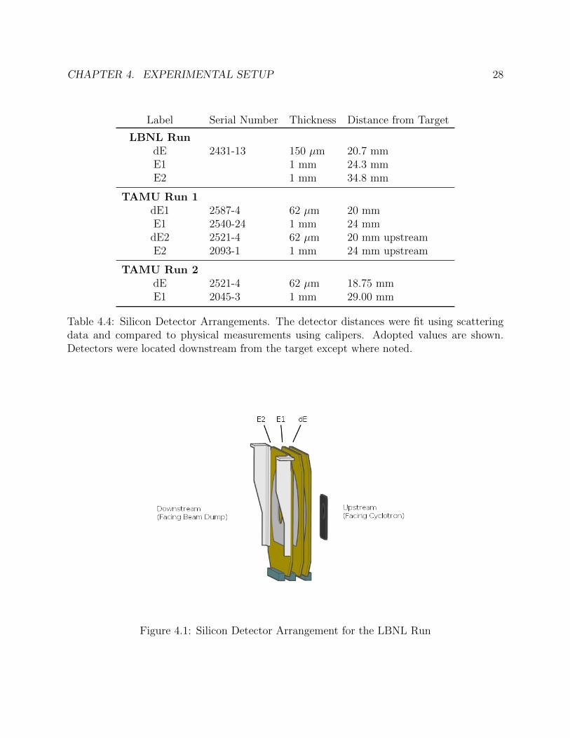
Micron Semiconductor “S2” type silicon detectors were used to detect and measure theoutgoing charged particles. These detectors are disk shaped, with a hole in the center forthe non-scattered beam to pass through. The silicon is divided into 48 rings and 16 sectorswhich allows for the (polar) angle from the beam and (azimuth) angle around the beam to berecorded. This segmentation also allows for a single detector to record multiple particle hits.The inner ring is located at a radius of 11 mm and the outer ring at 35 mm, making eachring 0.5 mm wide. The STARS chamber allows up to four of these detectors to be mountedand gives flexibility to the mounting position of each. A typical mounting arrangement is a“dE-E” arrangement. For this setup a thin (generally less than 150 µm) detector is placed infront of a thicker (generally 1 mm) detector. A scattered particle passes through the thinner“dE” detector, losing some of its energy, then deposits the rest in the thicker “E” detector.Since different particles lose energy at different rates for the same initial energy this setupcan be used to identify different charged particles assuming that they have enough energyto pass through the dE, and generally assuming they do not have enough energy to passthrough the E detector. The specific silicon setup for each run is shown in Table 4.4. Due tolimitations on the total number of channels, signals from adjacent rings and from adjacentsectors are often paired together resulting in a detector with 24 rings and 8 sectors. Thiswas done with all the detectors except for the dE detector in the second TAMU run.
CHAPTER 4. EXPERIMENTAL SETUP 28
Label Serial Number Thickness Distance from Target
LBNL RundE 2431-13 150 µm 20.7 mmE1 1 mm 24.3 mmE2 1 mm 34.8 mm
TAMU Run 1dE1 2587-4 62 µm 20 mmE1 2540-24 1 mm 24 mmdE2 2521-4 62 µm 20 mm upstreamE2 2093-1 1 mm 24 mm upstream
TAMU Run 2dE 2521-4 62 µm 18.75 mmE1 2045-3 1 mm 29.00 mm
Table 4.4: Silicon Detector Arrangements. The detector distances were fit using scatteringdata and compared to physical measurements using calipers. Adopted values are shown.Detectors were located downstream from the target except where noted.
Figure 4.1: Silicon Detector Arrangement for the LBNL Run
CHAPTER 4. EXPERIMENTAL SETUP 29
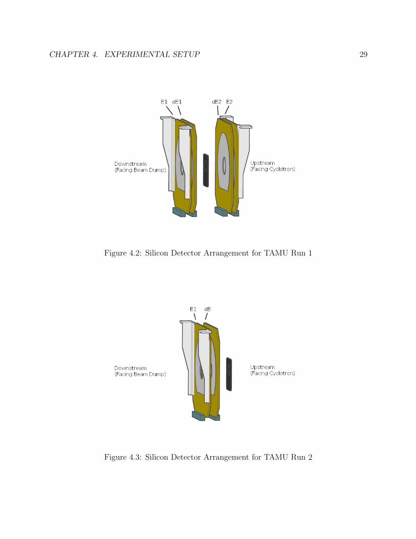
Figure 4.2: Silicon Detector Arrangement for TAMU Run 1
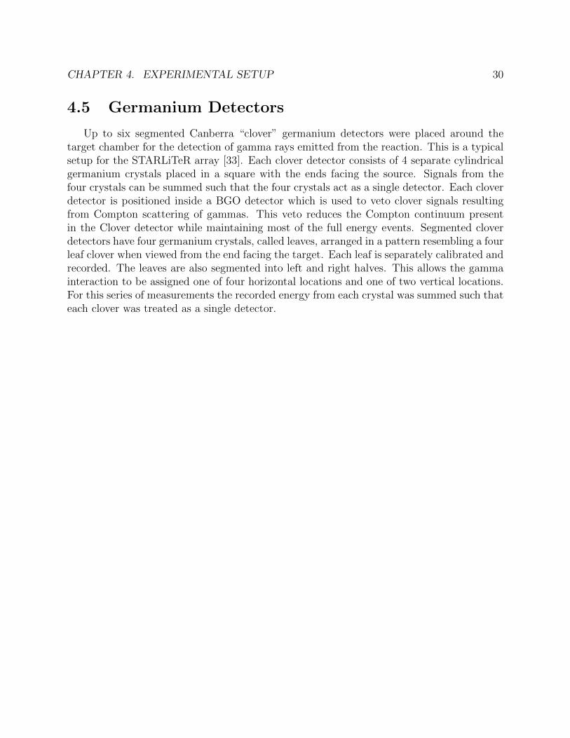
Figure 4.3: Silicon Detector Arrangement for TAMU Run 2
CHAPTER 4. EXPERIMENTAL SETUP 30
4.5 Germanium Detectors
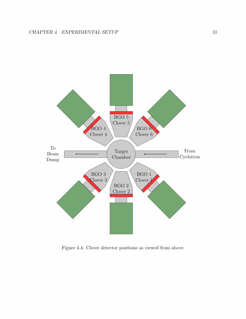
Up to six segmented Canberra “clover” germanium detectors were placed around thetarget chamber for the detection of gamma rays emitted from the reaction. This is a typicalsetup for the STARLiTeR array [33]. Each clover detector consists of 4 separate cylindricalgermanium crystals placed in a square with the ends facing the source. Signals from thefour crystals can be summed such that the four crystals act as a single detector. Each cloverdetector is positioned inside a BGO detector which is used to veto clover signals resultingfrom Compton scattering of gammas. This veto reduces the Compton continuum presentin the Clover detector while maintaining most of the full energy events. Segmented cloverdetectors have four germanium crystals, called leaves, arranged in a pattern resembling a fourleaf clover when viewed from the end facing the target. Each leaf is separately calibrated andrecorded. The leaves are also segmented into left and right halves. This allows the gammainteraction to be assigned one of four horizontal locations and one of two vertical locations.For this series of measurements the recorded energy from each crystal was summed such thateach clover was treated as a single detector.
CHAPTER 4. EXPERIMENTAL SETUP 31
ToBeamDump
FromCyclotron
TargetChamber
BGO 1Clover 1
BGO 2Clover 2
BGO 3Clover 3
BGO 4Clover 4
BGO 5Clover 5
BGO 6Clover 6
Figure 4.4: Clover detector positions as viewed from above.
CHAPTER 4. EXPERIMENTAL SETUP 32
Since the gamma rays of interest are emitted from nuclei that may have a recoil energy ofseveral MeV it is necessary to apply a Doppler correction to the detected gamma energy todetermine the gamma ray energy in the rest frame of the nucleus. For this purpose the twoupstream and two downstream detectors were considered to be at a 45 degree angle to thebeam and the final two detectors were at 90 degrees. These angles were within 5 degrees ofthe actual angle to the center of each detector from the target. This allowed for a sufficientDoppler correction to produce clean peaks in the gamma ray spectrum. The clover detectorarrangement is shown in Figure 4.4. The velocity used for the nucleus was that found forthe recoiling 24Mg nucleus. The 20Ne and 23Na nuclei receive an additional kick from theejected particle, but this generally a small change in velocity compared to the 24Mg recoilvelocity.
Most lines were well separated when they had sufficient counts to be visible. An importantexception is the 1634 keV line from the first excited state of 20Ne and the 1636 keV line fromthe second excited state of 23Na. It is unlikely that these lines could be resolved even withoutthe additional complication of the Doppler shift.
33
Chapter 5
Results and Analysis
5.1 24Mg Excitation Spectrum for Detected Events
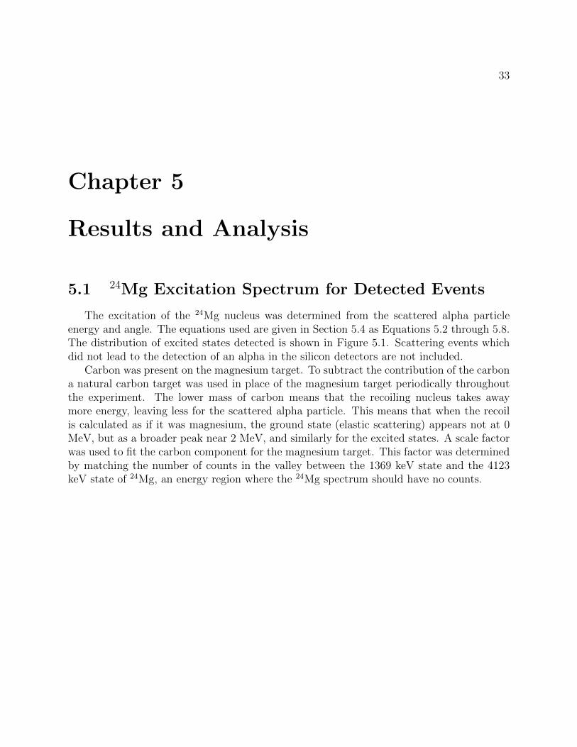
The excitation of the 24Mg nucleus was determined from the scattered alpha particleenergy and angle. The equations used are given in Section 5.4 as Equations 5.2 through 5.8.The distribution of excited states detected is shown in Figure 5.1. Scattering events whichdid not lead to the detection of an alpha in the silicon detectors are not included.
Carbon was present on the magnesium target. To subtract the contribution of the carbona natural carbon target was used in place of the magnesium target periodically throughoutthe experiment. The lower mass of carbon means that the recoiling nucleus takes awaymore energy, leaving less for the scattered alpha particle. This means that when the recoilis calculated as if it was magnesium, the ground state (elastic scattering) appears not at 0MeV, but as a broader peak near 2 MeV, and similarly for the excited states. A scale factorwas used to fit the carbon component for the magnesium target. This factor was determinedby matching the number of counts in the valley between the 1369 keV state and the 4123keV state of 24Mg, an energy region where the 24Mg spectrum should have no counts.
CHAPTER 5. RESULTS AND ANALYSIS 34
0
100000
200000
300000
400000
500000
600000
700000
800000
900000
0 5 10 15 20 25 30
counts
MeV
Mg24 Excitation from Detected Alphas
Elastic
1369 keVRegion ofinterestfor Gamowpeak
Mg target with C SubtractedMg target including C
C component of Mg target spectrum
Figure 5.1: The spectrum of excitation in 24Mg corresponding to detected alpha particles.This plot shows the contribution from 12C before and after having been subtracted.
5.2 Gamma Ray Spectrum
For many of the excited states in the product nuclei, requiring a coincidence with acharacteristic gamma allows a much cleaner identification of the outgoing channel. For thesecond and third excited states of 20Ne, the second, third, and fifth excited states of 23Na,and the first excited state of 23Mg the identification was made using a coincidence betweenthe scattered alpha and a characteristic gamma ray. The 2076 keV (second excited) state of23Na is fed by the fifth excited state requiring the fifth excited state to be determined priorto the second state and its contribution subtracted from the strength of the second state’scharacteristic gamma ray.
The ground state and first excited (440 keV) state of 23Na could not be well separatedfrom each other using particle data alone, though the pair was well separated from higherexcited states. The 440 keV gamma ray coincident with the first excited state was used toseparate the contributions of these two states.
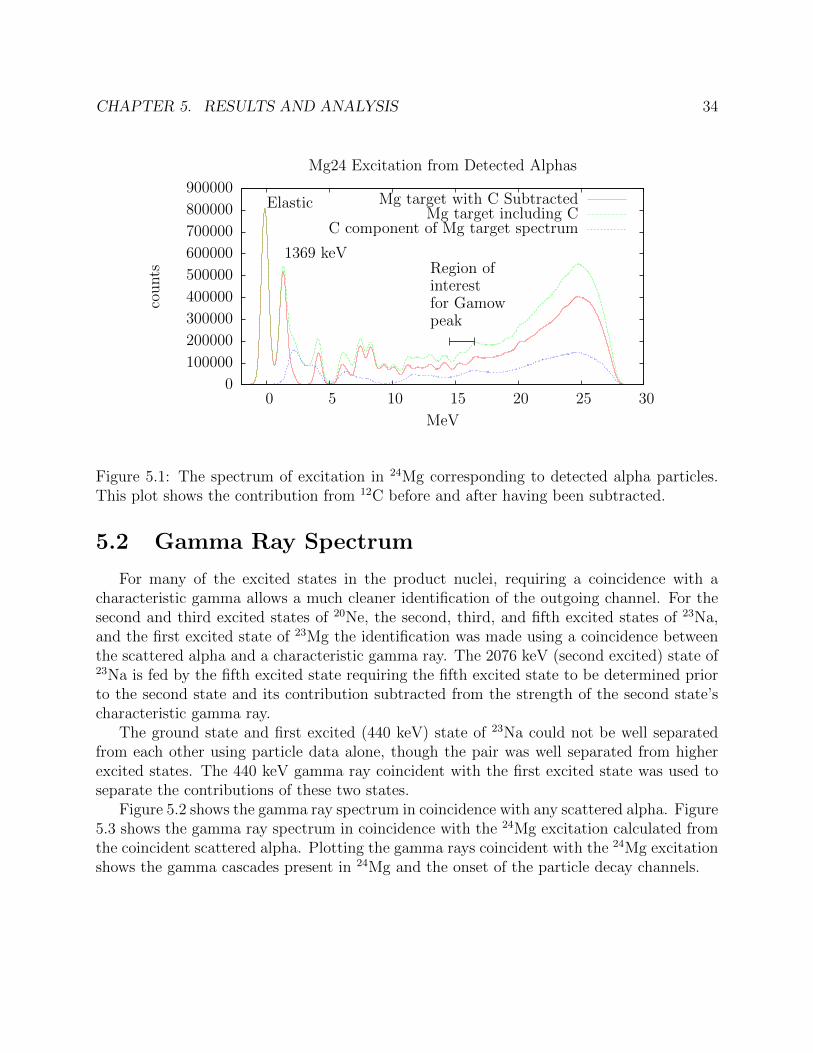
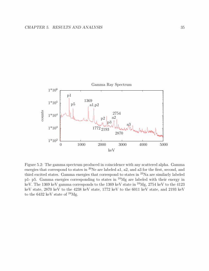
Figure 5.2 shows the gamma ray spectrum in coincidence with any scattered alpha. Figure5.3 shows the gamma ray spectrum in coincidence with the 24Mg excitation calculated fromthe coincident scattered alpha. Plotting the gamma rays coincident with the 24Mg excitationshows the gamma cascades present in 24Mg and the onset of the particle decay channels.
CHAPTER 5. RESULTS AND ANALYSIS 35
1*102
1*103
1*104
1*105
1*106
0 1000 2000 3000 4000 5000
counts
keV
Gamma Ray Spectrum
1369
p1
a1,p2
a2
a3
p2p3
p5
2754
28701772 2193
Figure 5.2: The gamma spectrum produced in coincidence with any scattered alpha. Gammaenergies that correspond to states in 20Ne are labeled a1, a2, and a3 for the first, second, andthird excited states. Gamma energies that correspond to states in 23Na are similarly labeledp1- p5. Gamma energies corresponding to states in 24Mg are labeled with their energy inkeV. The 1369 keV gamma corresponds to the 1369 keV state in 24Mg, 2754 keV to the 4123keV state, 2870 keV to the 4238 keV state, 1772 keV to the 6011 keV state, and 2193 keVto the 6432 keV state of 24Mg.
CHAPTER 5. RESULTS AND ANALYSIS 36
0
5
10
15
20
25
30
0 1000 2000 3000 4000 5000
Exci
tati
on(M
eV)
Gamma Energy (keV)
Gamma Ray Energy vs Mg24 Excitation from Scattered Alpha
0
500
1000
1500
2000
2500
Figure 5.3: The gamma ray energies vs the excitation of 24Mg as calculated from the coinci-dent scattered alpha. The 1369 keV gamma from the first excited state of 24Mg can bee seenstrongly at lower excitation energies as it is fed by many of the higher excited states. Ataround 13 to 14 MeV excitation it can be seen to diminish in favor of the 440 keV gammafrom 23Na and the 1634 keV gamma from 20Ne, showing the opening of the particle decaychannels at higher excitation energies.
CHAPTER 5. RESULTS AND ANALYSIS 37
5.3 Angular Distributions
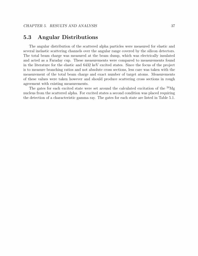
The angular distribution of the scattered alpha particles were measured for elastic andseveral inelastic scattering channels over the angular range covered by the silicon detectors.The total beam charge was measured at the beam dump, which was electrically insulatedand acted as a Faraday cup. These measurements were compared to measurements foundin the literature for the elastic and 6432 keV excited states. Since the focus of the projectis to measure branching ratios and not absolute cross sections, less care was taken with themeasurement of the total beam charge and exact number of target atoms. Measurementsof these values were taken however and should produce scattering cross sections in roughagreement with existing measurements.
The gates for each excited state were set around the calculated excitation of the 24Mgnucleus from the scattered alpha. For excited states a second condition was placed requiringthe detection of a characteristic gamma ray. The gates for each state are listed in Table 5.1.
CHAPTER 5. RESULTS AND ANALYSIS 38
24Mg State Minimum Maximum Characteristic Minimum MaximumExcitation Excitation Gamma Gamma Gamma
Energy EnergyGround (Elastic) - 0.7 MeV - - -
1368 keV 0.6 MeV 2.0 MeV 1368 keV 1350 keV 1390 keV4123 keV 3.4 MeV 4.8 MeV 2754 keV 2735 keV 2770 keV4238 keV 3.4 MeV 4.8 MeV 2870 keV 2850 keV 2885 keV6011 keV 5.3 MeV 6.8 MeV 1772 keV 1760 keV 1780 keV6432 keV 5.8 MeV 6.8 MeV 2193 keV 2180 keV 2205 keV
Table 5.1: The 24Mg excitation energy requirement and gamma ray energy requirement forthe identification of the 24Mg states.
0.1
1
10
100
30 35 40 45 50 55
mb/s
tr
Degrees (lab frame)
Elastic Scattering of Alphas on Mg24 (0+) Angular Cross Section
TAMU RunLBNL Run
J,IZV,32,604,1968
Figure 5.4: Elastic angular cross section. An existing data set taken at 40 MeV is shown forcomparison. Data points below 33 degrees for both the LBNL and TAMU runs as well asdata points above 47 degrees for the TAMU run and 53 degrees for the LBNL run fall offdue to the edge of the detector and should not be considered valid. The error bars for theTAMU and LBNL runs denote statistical uncertainty only.
CHAPTER 5. RESULTS AND ANALYSIS 39
0.1
1
10
30 35 40 45 50 55
mb/s
tr
Degrees (lab frame)
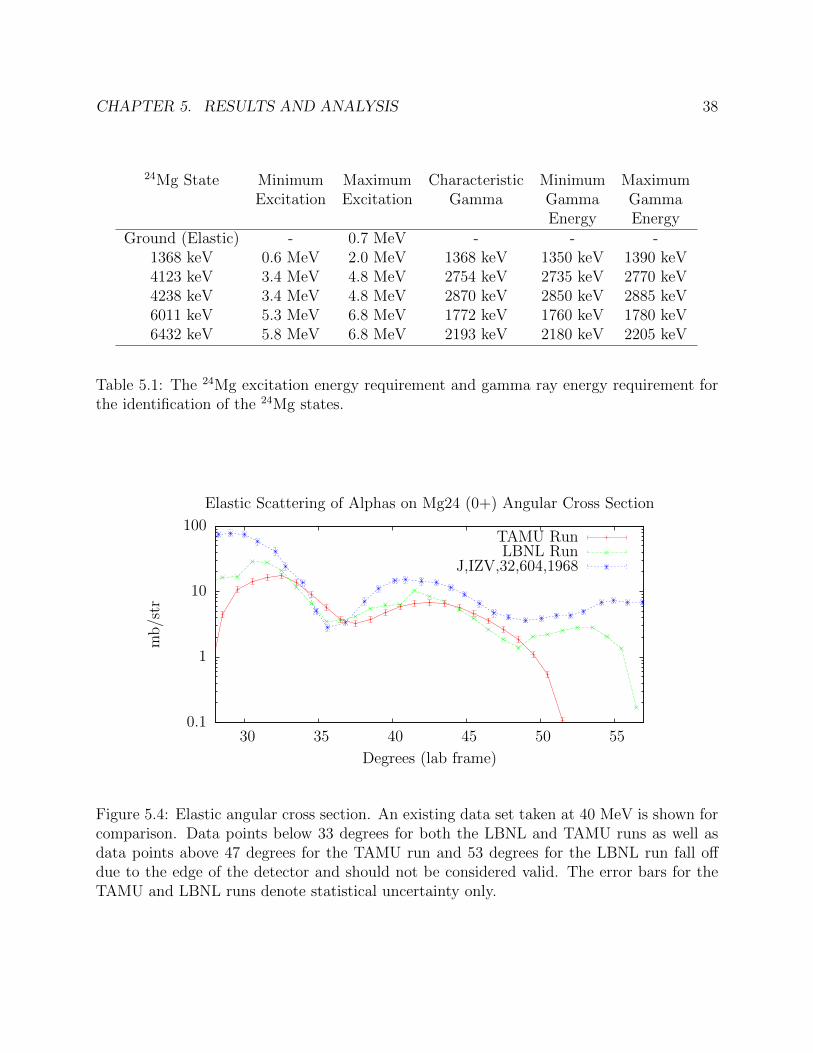
1368 keV State of Mg24 (2+) Inelastic Alpha Scattering
TAMU Run
Figure 5.5: Inelastic scattering cross section for the 1368 keV excited state of 24Mg. Data isshown in the lab frame of reference. The error bars denote statistical uncertainty only.
0.1
1
10
30 35 40 45 50 55
mb/s
tr
Degrees (lab frame)
4123 keV State of Mg24 (4+) Inelastic Alpha Scattering
TAMU Run
Figure 5.6: Inelastic scattering cross section for the 4123 keV excited state of 24Mg. Data isshown in the lab frame of reference. The error bars denote statistical uncertainty only.
CHAPTER 5. RESULTS AND ANALYSIS 40
0.1
1
10
30 35 40 45 50 55
mb/s
tr
Degrees (lab frame)
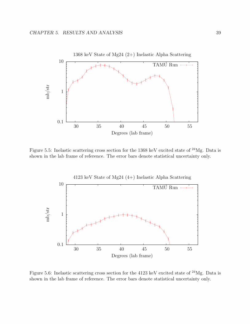
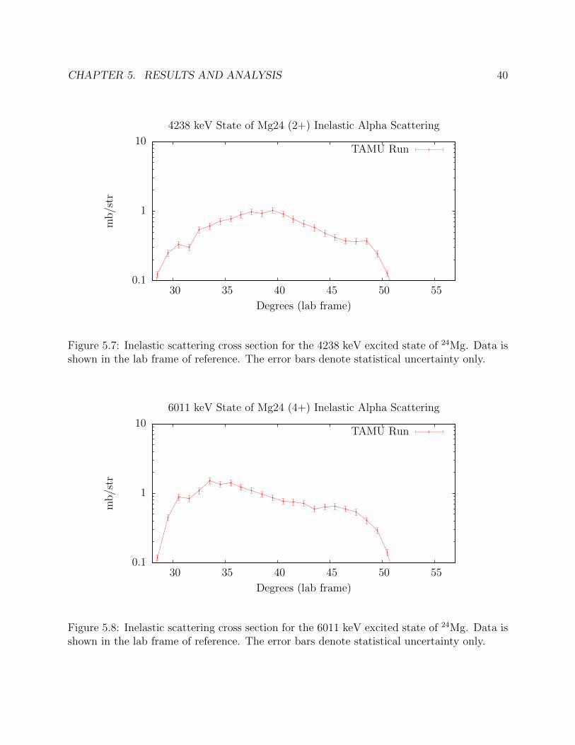
4238 keV State of Mg24 (2+) Inelastic Alpha Scattering
TAMU Run
Figure 5.7: Inelastic scattering cross section for the 4238 keV excited state of 24Mg. Data isshown in the lab frame of reference. The error bars denote statistical uncertainty only.
0.1
1
10
30 35 40 45 50 55
mb/s
tr
Degrees (lab frame)
6011 keV State of Mg24 (4+) Inelastic Alpha Scattering
TAMU Run
Figure 5.8: Inelastic scattering cross section for the 6011 keV excited state of 24Mg. Data isshown in the lab frame of reference. The error bars denote statistical uncertainty only.
CHAPTER 5. RESULTS AND ANALYSIS 41
0.1
1
10
30 35 40 45 50 55
mb/s
tr
Degrees (lab frame)
6432 keV State of Mg24 (0+) Inelastic Alpha Scattering
TAMU RunJ.PR/C 33 40 1986
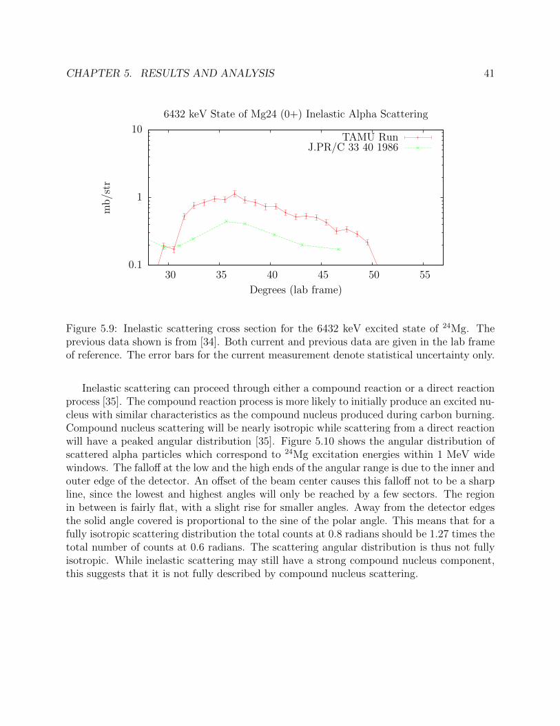
Figure 5.9: Inelastic scattering cross section for the 6432 keV excited state of 24Mg. Theprevious data shown is from [34]. Both current and previous data are given in the lab frameof reference. The error bars for the current measurement denote statistical uncertainty only.
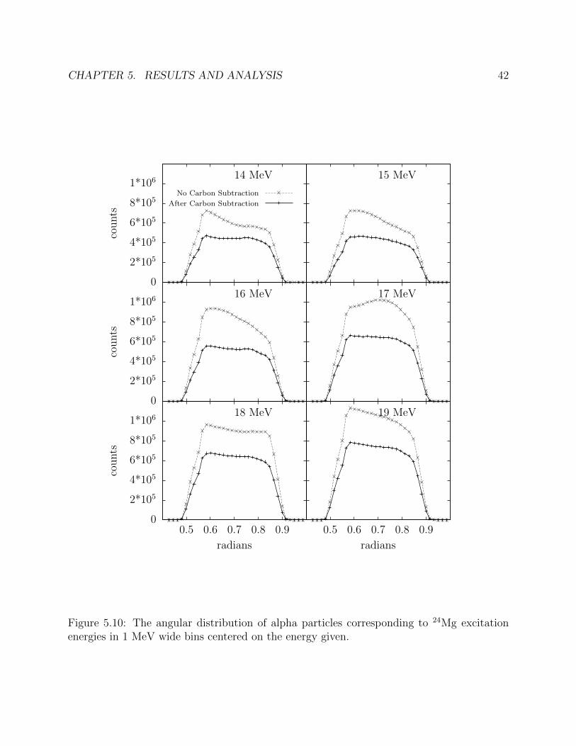
Inelastic scattering can proceed through either a compound reaction or a direct reactionprocess [35]. The compound reaction process is more likely to initially produce an excited nu-cleus with similar characteristics as the compound nucleus produced during carbon burning.Compound nucleus scattering will be nearly isotropic while scattering from a direct reactionwill have a peaked angular distribution [35]. Figure 5.10 shows the angular distribution ofscattered alpha particles which correspond to 24Mg excitation energies within 1 MeV widewindows. The falloff at the low and the high ends of the angular range is due to the inner andouter edge of the detector. An offset of the beam center causes this falloff not to be a sharpline, since the lowest and highest angles will only be reached by a few sectors. The regionin between is fairly flat, with a slight rise for smaller angles. Away from the detector edgesthe solid angle covered is proportional to the sine of the polar angle. This means that for afully isotropic scattering distribution the total counts at 0.8 radians should be 1.27 times thetotal number of counts at 0.6 radians. The scattering angular distribution is thus not fullyisotropic. While inelastic scattering may still have a strong compound nucleus component,this suggests that it is not fully described by compound nucleus scattering.
CHAPTER 5. RESULTS AND ANALYSIS 42
0
2*105
4*105
6*105
8*105
1*106
counts
14 MeV 15 MeV
0
2*105
4*105
6*105
8*105
1*106
counts
16 MeV 17 MeV
0
2*105
4*105
6*105
8*105
1*106
0.5 0.6 0.7 0.8 0.9
counts
radians
18 MeV
0.5 0.6 0.7 0.8 0.9
radians
19 MeV
No Carbon Subtraction
After Carbon Subtraction
Figure 5.10: The angular distribution of alpha particles corresponding to 24Mg excitationenergies in 1 MeV wide bins centered on the energy given.
CHAPTER 5. RESULTS AND ANALYSIS 43
5.4 Channel Identification and Branching Ratios
Identifying the excitation produced in the 24Mg nucleus, the daughter nucleus produced,and the excitation of the daughter nucleus relies on the scattered alpha particle from thebeam and the emitted particles and gammas from the excited 24Mg. The scattered andejected alpha particles and protons are detected using the silicon detectors located inside thetarget chamber.
The electrical contacts on each silicon detector are divided into 48 rings on one side and16 sectors on the other, with each ring and sector connected to its own preamp and ADC.The 16 sectors combined make a complete circle around the beam. The inner ring is locatedat a radius of 11 mm and each ring is 0.5 mm wide, with the last ring at a radius of 35 mm.Ideally a particle will produce a signal across one ring and one sector, though in practicesmall signals are often generated on neighboring rings either due to cross talk or occasionallydue to a particle entering near the boundary between two rings. For the LBNL run and thefirst TAMU run adjacent rings and adjacent sectors were connected prior to the preamps toproduce a detector with 24 ring pairs and 8 sector pairs. This was also done for the thickerE detector in the second TAMU run. This was done to reduce the number of ADC channelsneeded to read out the detectors. Timing (TAC) channels were also connected to rings andsectors individually, though due to a limit on the total number of TAC channels only selectedrings and sectors were connected to a TAC. All rings and sectors of the dE silicon detectorwere connected to a TAC, while the E detector had all sectors connected to a TAC. TheTAC was used to tighten the required coincidence timing window to reduce the total numberof random coincidences.
The energy readings for each ring and sector were calibrated individually using a 226Rasource. Silicon detectors have a near 100% efficiency for charged particles at the energiesof interest that hit active areas of the detector. The efficiency of each detector is thenapproximately the solid angle covered by the active area of the detector. A Monte Carlocode was used to model the final efficiency for detecting each particle. This approach was usedso that the forward scattering of the particles would be accounted for as well as situationssuch as a particle passing through the thinner dE detector but missing the thicker E detectorbehind it, as might happen for particles hitting the outer rings of the dE detector.
All detectors were read out when a “master gate” was produced. A master gate wasproduced when the downstream dE detector (labeled dE1 for the first TAMU run, dE forthe LBNL and second TAMU runs) and the downstream E detector (labeled E1 for theLBNL run and the first TAMU run, E for the second TAMU run) each had at least one ringor sector signal above a threshold corresponding to approximately 500 keV.
Signals from the rings and sectors were compared while sorting the data to determinewhich pixels (overlaps of ring and sector) were hit. The pairing was done by comparingthe calibrated energy of each ring to each sector. The ring with the energy closest to thesector was considered to be the matching ring for that hit. Rings with an energy more than700 keV different from the sector were not considered. If adjacent rings fired their sum
CHAPTER 5. RESULTS AND ANALYSIS 44
Decay Reaction Main Alpha Energy Branch Half Life226Ra(α)222Rn 4784.34 keV 100% 1600 years222Rn(α)218Po 5489.48 keV 100% 3.8235 days218Po(α)214Pb 6002.35 keV 99.980% 3.098 minutes
214Pb(β−)214Bi 100% 26.8 minutes214Bi(β1)214Po 99.98% 19.9 minutes214Po(α)210Pb 7686.82 keV 100% 163.4 microseconds
210Pb(β−)210Bi 100% 22.20 years210Bi(β−)210Po 100% 2.012 days210Po(α)206Pb 5304.33 keV 100% 138.376 days
206Pb Stable
Table 5.2: The decay chain for 226Ra. The first four alpha peaks in the decay chain were insecular equilibrium since the half lives of 222Rn through 214Po are all much less than the ageof the source. The source was not old enough for 210Pb to be in secular equilibrium yet andas a result the 5.3 MeV Peak from 210Po was small and not used for calibrations. Data isfrom the NNDC website[29].
was compared to the sector in a similar way, with the higher energy ring being assignedas the corresponding ring to the hit sector. Once the corresponding ring was found for asector, the adjacent rings were removed from the search for other sectors that might havefired. This process started with the highest energy sector and proceeded to lower energysectors in order. Multiple hits within a single event were common, and necessary for theparticle-particle coincidence measurements.
Pixels for the dE and E detectors were paired based on a ray trace window. First, thesector for the dE hit had to overlap the sector for the E hit. Second, each E detector ringpair was assigned 5 acceptable dE rings, the center of which was in line with the center of thetarget. If both criteria were satisfied, these signals were considered to have been producedby a single particle passing through the dE and hitting the E detector behind it. Signalsthat corresponded to a dE hit that was not paired to a E1 hit were kept since these hits maybe particles with a low enough energy that they did not pass through the dE detector. Edetector hits that did not have a corresponding dE detector hit were discarded.
Once a dE and an E hit were paired, their energies were used to determine what typeof particle they were. Different charged particles lose energy at different rates while passingthough the dE detector and this can be used to identify protons and alpha particles. Somedeuterons and tritons were also identified this way and this identification was used to discardthose events. Figure 5.11 shows the measured energy loss in the dE detector divided by thepath length of the particle in the dE detector for particles of different total energy. Dividingby the path length accounts for the greater amount of energy a particle at a high angle would
CHAPTER 5. RESULTS AND ANALYSIS 45
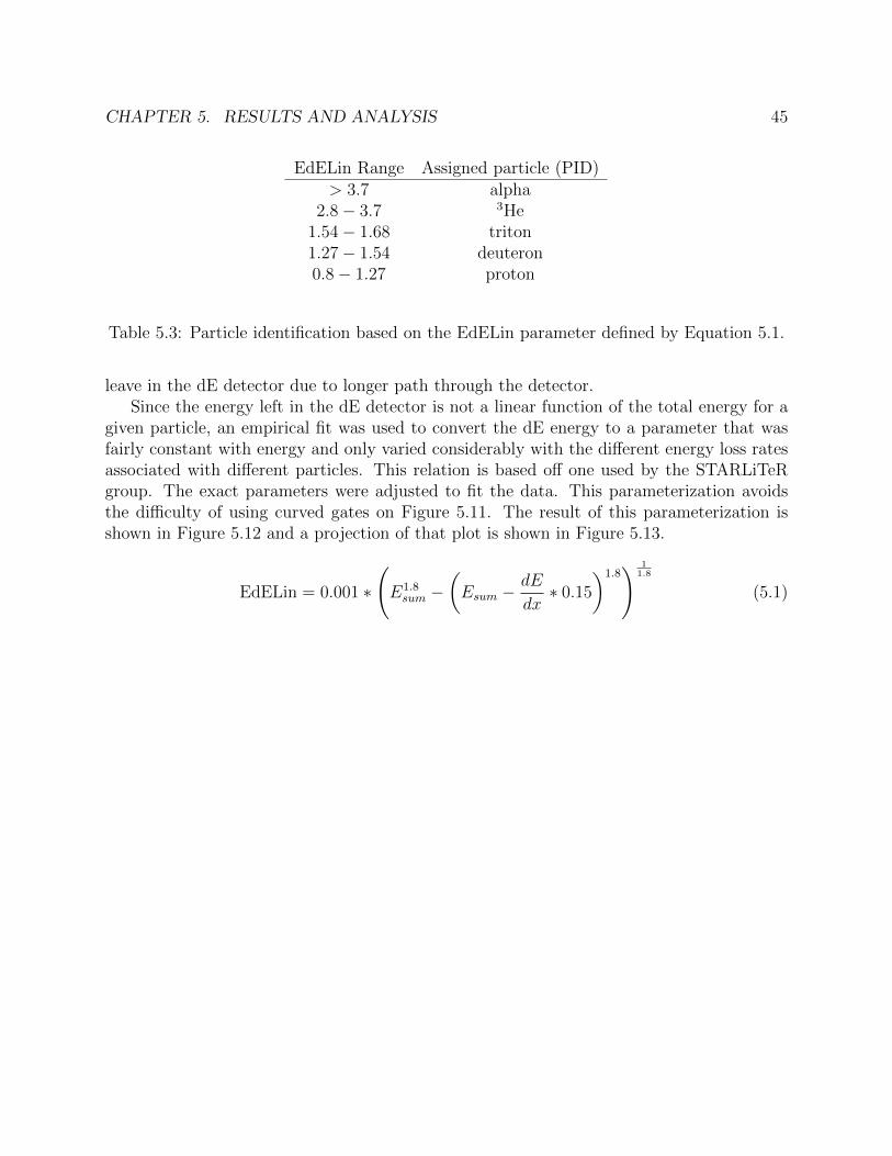
EdELin Range Assigned particle (PID)> 3.7 alpha
2.8− 3.7 3He1.54− 1.68 triton1.27− 1.54 deuteron0.8− 1.27 proton
Table 5.3: Particle identification based on the EdELin parameter defined by Equation 5.1.
leave in the dE detector due to longer path through the detector.Since the energy left in the dE detector is not a linear function of the total energy for a
given particle, an empirical fit was used to convert the dE energy to a parameter that wasfairly constant with energy and only varied considerably with the different energy loss ratesassociated with different particles. This relation is based off one used by the STARLiTeRgroup. The exact parameters were adjusted to fit the data. This parameterization avoidsthe difficulty of using curved gates on Figure 5.11. The result of this parameterization isshown in Figure 5.12 and a projection of that plot is shown in Figure 5.13.
EdELin = 0.001 ∗
(E1.8sum −
(Esum −
dE
dx∗ 0.15
)1.8) 1
1.8
(5.1)
CHAPTER 5. RESULTS AND ANALYSIS 46
0
20
40
60
80
100
120
0 5 10 15 20 25 30 35 40
Ener
gyL
oss
Rat
e(M
eV/u
m)
Total Energy (MeV)
Energy Loss Rate in the dE Detector vs Total Particle E
p
d
alpha
0
200000
400000
600000
800000
1e+006
p
d
alpha
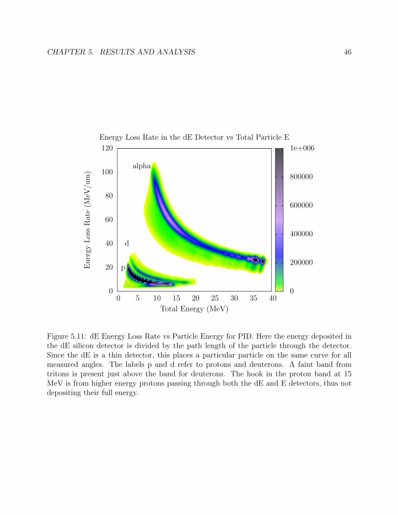
Figure 5.11: dE Energy Loss Rate vs Particle Energy for PID. Here the energy deposited inthe dE silicon detector is divided by the path length of the particle through the detector.Since the dE is a thin detector, this places a particular particle on the same curve for allmeasured angles. The labels p and d refer to protons and deuterons. A faint band fromtritons is present just above the band for deuterons. The hook in the proton band at 15MeV is from higher energy protons passing through both the dE and E detectors, thus notdepositing their full energy.
CHAPTER 5. RESULTS AND ANALYSIS 47
0
1
2
3
4
5
0 5 10 15 20 25 30 35 40
PID
Par
amet
er
Total Energy (MeV)
Linearized PID Parameter vs Total Particle PID
pd
t
alpha
0
100000
200000
300000
400000
500000
pd
t
alpha
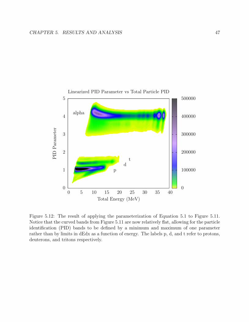
Figure 5.12: The result of applying the parameterization of Equation 5.1 to Figure 5.11.Notice that the curved bands from Figure 5.11 are now relatively flat, allowing for the particleidentification (PID) bands to be defined by a minimum and maximum of one parameterrather than by limits in dEdx as a function of energy. The labels p, d, and t refer to protons,deuterons, and tritons respectively.
CHAPTER 5. RESULTS AND ANALYSIS 48
0
1e+007
2e+007
3e+007
4e+007
5e+007
6e+007
7e+007
8e+007
0 1 2 3 4 5
counts
Linearized PID
Linearized PID Projection
p
d
alpha
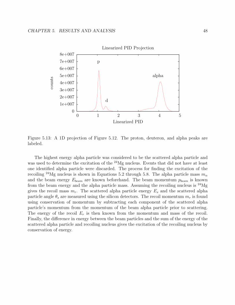
Figure 5.13: A 1D projection of Figure 5.12. The proton, deuteron, and alpha peaks arelabeled.
The highest energy alpha particle was considered to be the scattered alpha particle andwas used to determine the excitation of the 24Mg nucleus. Events that did not have at leastone identified alpha particle were discarded. The process for finding the excitation of therecoiling 24Mg nucleus is shown in Equations 5.2 through 5.8. The alpha particle mass mα
and the beam energy Ebeam are known beforehand. The beam momentum pbeam is knownfrom the beam energy and the alpha particle mass. Assuming the recoiling nucleus is 24Mggives the recoil mass mr. The scattered alpha particle energy Es and the scattered alphaparticle angle θs are measured using the silicon detectors. The recoil momentum mr is foundusing conservation of momentum by subtracting each component of the scattered alphaparticle’s momentum from the momentum of the beam alpha particle prior to scattering.The energy of the recoil Er is then known from the momentum and mass of the recoil.Finally, the difference in energy between the beam particles and the sum of the energy of thescattered alpha particle and recoiling nucleus gives the excitation of the recoiling nucleus byconservation of energy.
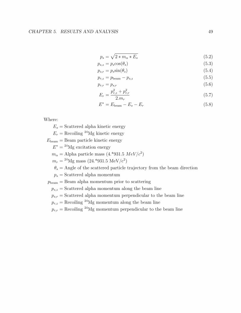
CHAPTER 5. RESULTS AND ANALYSIS 49
ps =√
2 ∗mα ∗ Es (5.2)
ps,z = pscos(θs) (5.3)
ps,r = pssin(θs) (5.4)
pr,z = pbeam − ps,z (5.5)
pr,r = ps,r (5.6)
Er =p2r,z + p2
r,r
2.mr
(5.7)
E∗ = Ebeam − Es − Er (5.8)
Where:
Es = Scattered alpha kinetic energy
Er = Recoiling 24Mg kinetic energy
Ebeam = Beam particle kinetic energy
E∗ = 24Mg excitation energy
mα = Alpha particle mass (4.*931.5 MeV/c2)
mr = 24Mg mass (24.*931.5 MeV/c2)
θs = Angle of the scattered particle trajectory from the beam direction
ps = Scattered alpha momentum
pbeam = Beam alpha momentum prior to scattering
ps,z = Scattered alpha momentum along the beam line
ps,r = Scattered alpha momentum perpendicular to the beam line
pr,z = Recoiling 24Mg momentum along the beam line
pr,r = Recoiling 24Mg momentum perpendicular to the beam line
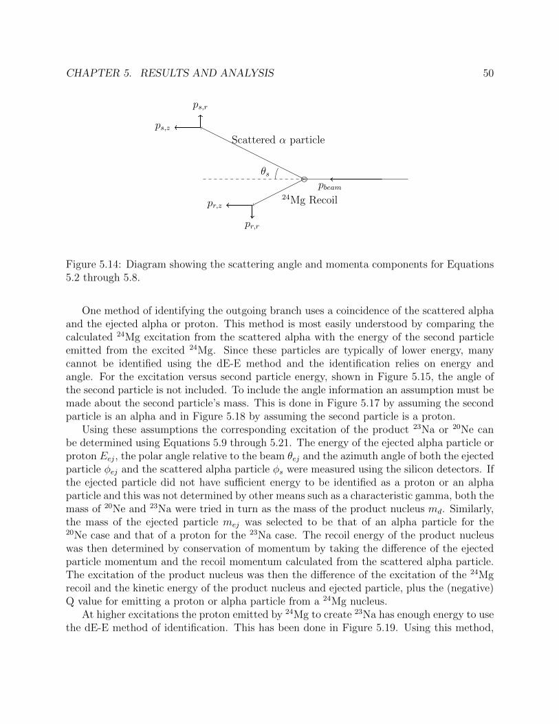
CHAPTER 5. RESULTS AND ANALYSIS 50
pbeam
θs
Scattered α particle
ps,z
ps,r
pr,z
pr,r
24Mg Recoil
Figure 5.14: Diagram showing the scattering angle and momenta components for Equations5.2 through 5.8.
One method of identifying the outgoing branch uses a coincidence of the scattered alphaand the ejected alpha or proton. This method is most easily understood by comparing thecalculated 24Mg excitation from the scattered alpha with the energy of the second particleemitted from the excited 24Mg. Since these particles are typically of lower energy, manycannot be identified using the dE-E method and the identification relies on energy andangle. For the excitation versus second particle energy, shown in Figure 5.15, the angle ofthe second particle is not included. To include the angle information an assumption must bemade about the second particle’s mass. This is done in Figure 5.17 by assuming the secondparticle is an alpha and in Figure 5.18 by assuming the second particle is a proton.
Using these assumptions the corresponding excitation of the product 23Na or 20Ne canbe determined using Equations 5.9 through 5.21. The energy of the ejected alpha particle orproton Eej, the polar angle relative to the beam θej and the azimuth angle of both the ejectedparticle φej and the scattered alpha particle φs were measured using the silicon detectors. Ifthe ejected particle did not have sufficient energy to be identified as a proton or an alphaparticle and this was not determined by other means such as a characteristic gamma, both themass of 20Ne and 23Na were tried in turn as the mass of the product nucleus md. Similarly,the mass of the ejected particle mej was selected to be that of an alpha particle for the20Ne case and that of a proton for the 23Na case. The recoil energy of the product nucleuswas then determined by conservation of momentum by taking the difference of the ejectedparticle momentum and the recoil momentum calculated from the scattered alpha particle.The excitation of the product nucleus was then the difference of the excitation of the 24Mgrecoil and the kinetic energy of the product nucleus and ejected particle, plus the (negative)Q value for emitting a proton or alpha particle from a 24Mg nucleus.
At higher excitations the proton emitted by 24Mg to create 23Na has enough energy to usethe dE-E method of identification. This has been done in Figure 5.19. Using this method,
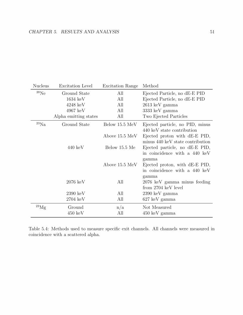
CHAPTER 5. RESULTS AND ANALYSIS 51
Nucleus Excitation Level Excitation Range Method20Ne Ground State All Ejected Particle, no dE-E PID
1634 keV All Ejected Particle, no dE-E PID4248 keV All 2613 keV gamma4967 keV All 3333 keV gamma
Alpha emitting states All Two Ejected Particles
23Na Ground State Below 15.5 MeV Ejected particle, no PID, minus440 keV state contribution
Above 15.5 MeV Ejected proton with dE-E PID,minus 440 keV state contribution
440 keV Below 15.5 Me Ejected particle, no dE-E PID,in coincidence with a 440 keVgamma
Above 15.5 MeV Ejected proton, with dE-E PID,in coincidence with a 440 keVgamma
2076 keV All 2076 keV gamma minus feedingfrom 2704 keV level
2390 keV All 2390 keV gamma2704 keV All 627 keV gamma
23Mg Ground n/a Not Measured450 keV All 450 keV gamma
Table 5.4: Methods used to measure specific exit channels. All channels were measured incoincidence with a scattered alpha.
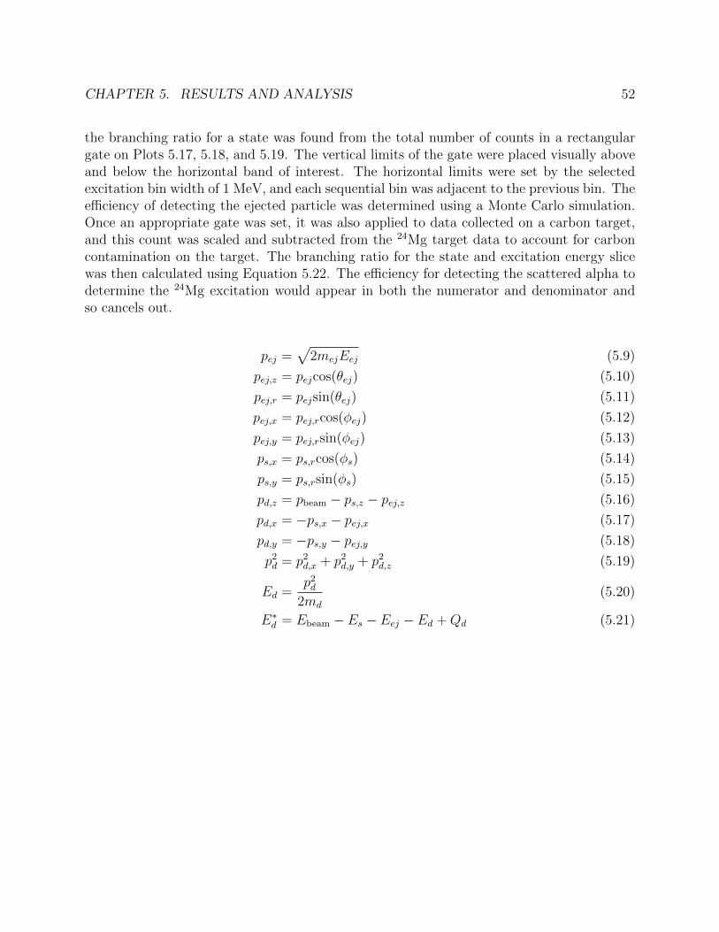
CHAPTER 5. RESULTS AND ANALYSIS 52
the branching ratio for a state was found from the total number of counts in a rectangulargate on Plots 5.17, 5.18, and 5.19. The vertical limits of the gate were placed visually aboveand below the horizontal band of interest. The horizontal limits were set by the selectedexcitation bin width of 1 MeV, and each sequential bin was adjacent to the previous bin. Theefficiency of detecting the ejected particle was determined using a Monte Carlo simulation.Once an appropriate gate was set, it was also applied to data collected on a carbon target,and this count was scaled and subtracted from the 24Mg target data to account for carboncontamination on the target. The branching ratio for the state and excitation energy slicewas then calculated using Equation 5.22. The efficiency for detecting the scattered alpha todetermine the 24Mg excitation would appear in both the numerator and denominator andso cancels out.
pej =√
2mejEej (5.9)
pej,z = pejcos(θej) (5.10)
pej,r = pejsin(θej) (5.11)
pej,x = pej,rcos(φej) (5.12)
pej,y = pej,rsin(φej) (5.13)
ps,x = ps,rcos(φs) (5.14)
ps,y = ps,rsin(φs) (5.15)
pd,z = pbeam − ps,z − pej,z (5.16)
pd,x = −ps,x − pej,x (5.17)
pd,y = −ps,y − pej,y (5.18)
p2d = p2
d,x + p2d,y + p2
d,z (5.19)
Ed =p2d
2md
(5.20)
E∗d = Ebeam − Es − Eej − Ed +Qd (5.21)
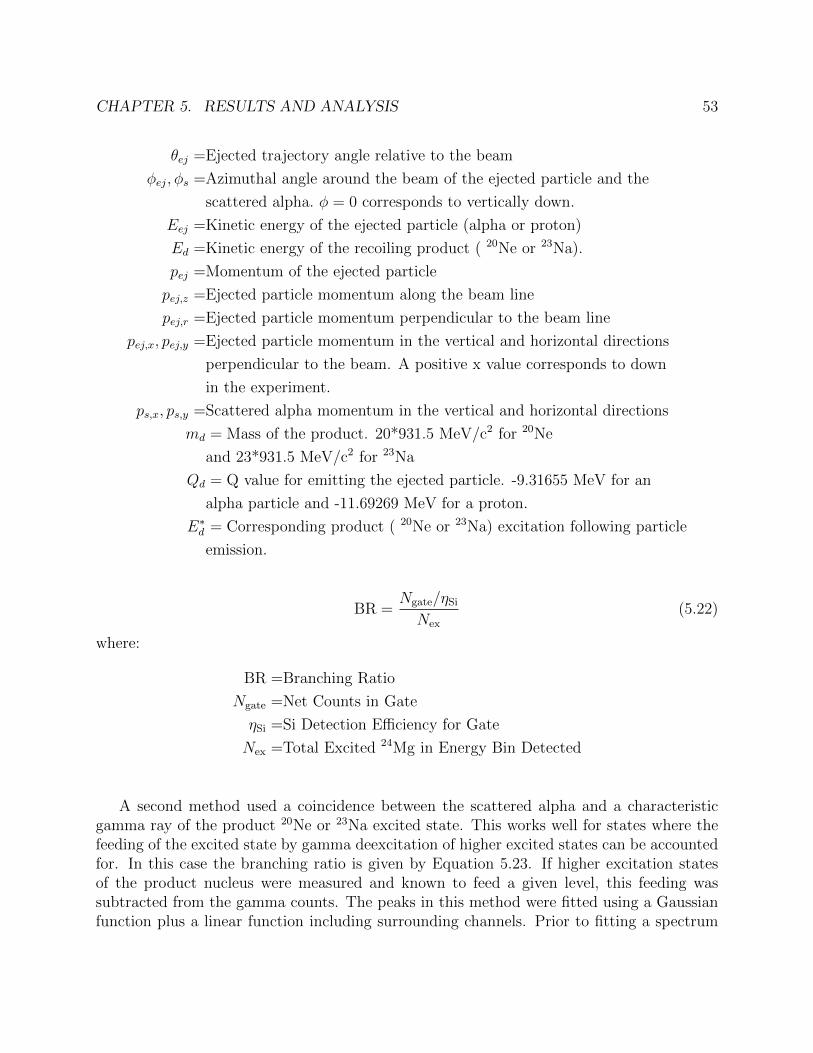
CHAPTER 5. RESULTS AND ANALYSIS 53
θej =Ejected trajectory angle relative to the beam
φej, φs =Azimuthal angle around the beam of the ejected particle and the
scattered alpha. φ = 0 corresponds to vertically down.
Eej =Kinetic energy of the ejected particle (alpha or proton)
Ed =Kinetic energy of the recoiling product ( 20Ne or 23Na).
pej =Momentum of the ejected particle
pej,z =Ejected particle momentum along the beam line
pej,r =Ejected particle momentum perpendicular to the beam line
pej,x, pej,y =Ejected particle momentum in the vertical and horizontal directions
perpendicular to the beam. A positive x value corresponds to down
in the experiment.
ps,x, ps,y =Scattered alpha momentum in the vertical and horizontal directions
md = Mass of the product. 20*931.5 MeV/c2 for 20Ne
and 23*931.5 MeV/c2 for 23Na
Qd = Q value for emitting the ejected particle. -9.31655 MeV for an
alpha particle and -11.69269 MeV for a proton.
E∗d = Corresponding product ( 20Ne or 23Na) excitation following particle
emission.
BR =Ngate/ηSi
Nex
(5.22)
where:
BR =Branching Ratio
Ngate =Net Counts in Gate
ηSi =Si Detection Efficiency for Gate
Nex =Total Excited 24Mg in Energy Bin Detected
A second method used a coincidence between the scattered alpha and a characteristicgamma ray of the product 20Ne or 23Na excited state. This works well for states where thefeeding of the excited state by gamma deexcitation of higher excited states can be accountedfor. In this case the branching ratio is given by Equation 5.23. If higher excitation statesof the product nucleus were measured and known to feed a given level, this feeding wassubtracted from the gamma counts. The peaks in this method were fitted using a Gaussianfunction plus a linear function including surrounding channels. Prior to fitting a spectrum
CHAPTER 5. RESULTS AND ANALYSIS 54
taken from the carbon target was subtracted. Since this spectrum did not have the samepeaks, this resulted only in a slight reduction to the background counts and did not have astrong affect on the number of counts attributed to the peak.
BR =Npeak/ηGe
Nex
(5.23)
where:
Npeak =Net Counts in Gamma Peak
ηGe =Peak Efficiency of the Clover Array for that Gamma
A particle-particle-gamma method was used to separate states that were not clearlyseparated using the particle method and had sufficient gamma feeding from higher excitationlevels to make the scattered alpha-characteristic gamma coincidence alone difficult to correct.The additional coincidence made the separation of the state very specific, but also reducedthe available statistics since both the ejected particle detection efficiency and the cloverarray efficiency had an effect. For this method the gate was set in the same method as thescattered alpha-ejected particle method with the addition of a gate around a characteristicgamma emitted by the excited state of interest. The branching ratio for this method is givenby Equation 5.24.
BR =Ngate/ (ηSi ∗ ηGe)
Nex
(5.24)
Finally, higher excited states of 20Ne decay by alpha decay, which makes the abovemethods difficult. The Q-value for 20Ne to emit an alpha particle is -4.73 MeV, and thefirst excited state to primarily decay by alpha emission is at 5.62 MeV. For this and higherstates a coincidence between the scattered alpha and two more particle hits was required.The efficiency of the silicon detectors to detect both ejected alpha particles was determinedusing a Monte Carlo simulation. The result is close to, but not exactly the efficiency fordetecting one ejected alpha squared. Part of this deviation is due to separate particle hits ina single sector not being distinguished from each other. This decision was made in order touse the sector detector energy as the particle energy. The other is due to slight differencesin the kinematic forward focusing. The branching ratio is determined by Equation 5.25. Allalpha emitting states were measured together for each 24Mg excitation slice.
BR =N2ej/ηSi,2ej
Nex
(5.25)
where:
N2ej =Number of 2 ejected particle events counted
ηSi,2ej =Silicon efficiency to detect two ejected particles
CHAPTER 5. RESULTS AND ANALYSIS 55
The method used for each state, the gammas used in the gate and whether the ejectedparticle was required to pass through the dE detector to provide a dE-E particle identificationis given in Table 5.4.
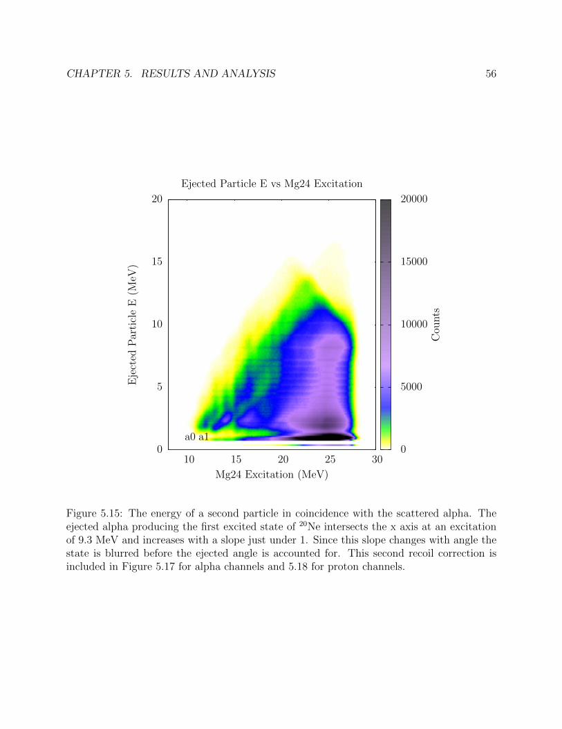
CHAPTER 5. RESULTS AND ANALYSIS 56
0
5
10
15
20
10 15 20 25 30
Eje
cted
Par
ticl
eE
(MeV
)
Mg24 Excitation (MeV)
Ejected Particle E vs Mg24 Excitation
0
5000
10000
15000
20000
Cou
nts
a0 a1
Figure 5.15: The energy of a second particle in coincidence with the scattered alpha. Theejected alpha producing the first excited state of 20Ne intersects the x axis at an excitationof 9.3 MeV and increases with a slope just under 1. Since this slope changes with angle thestate is blurred before the ejected angle is accounted for. This second recoil correction isincluded in Figure 5.17 for alpha channels and 5.18 for proton channels.
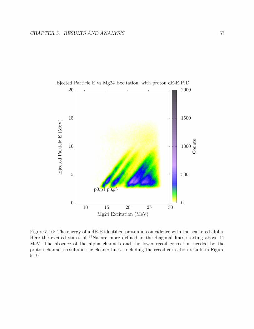
CHAPTER 5. RESULTS AND ANALYSIS 57
0
5
10
15
20
10 15 20 25 30
Eje
cted
Par
ticl
eE
(MeV
)
Mg24 Excitation (MeV)
Ejected Particle E vs Mg24 Excitation, with proton dE-E PID
0
500
1000
1500
2000
Cou
nts
p0,p1 p3,p5
Figure 5.16: The energy of a dE-E identified proton in coincidence with the scattered alpha.Here the excited states of 23Na are more defined in the diagonal lines starting above 11MeV. The absence of the alpha channels and the lower recoil correction needed by theproton channels results in the cleaner lines. Including the recoil correction results in Figure5.19.
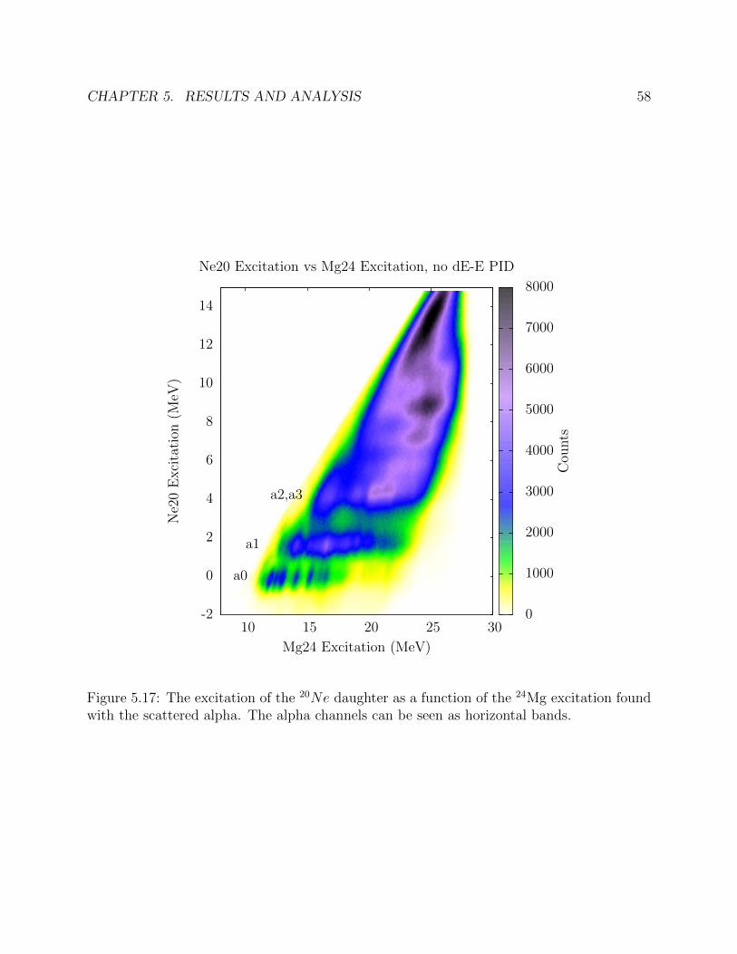
CHAPTER 5. RESULTS AND ANALYSIS 58
-2
0
2
4
6
8
10
12
14
10 15 20 25 30
Ne2
0E
xci
tati
on(M
eV)
Mg24 Excitation (MeV)
Ne20 Excitation vs Mg24 Excitation, no dE-E PID
0
1000
2000
3000
4000
5000
6000
7000
8000
Cou
nts
a0
a1
a2,a3
Figure 5.17: The excitation of the 20Ne daughter as a function of the 24Mg excitation foundwith the scattered alpha. The alpha channels can be seen as horizontal bands.
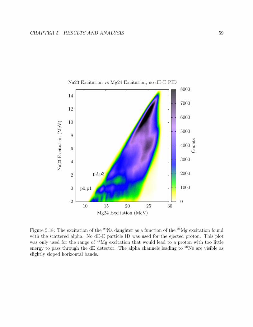
CHAPTER 5. RESULTS AND ANALYSIS 59
-2
0
2
4
6
8
10
12
14
10 15 20 25 30
Na2
3E
xci
tati
on(M
eV)
Mg24 Excitation (MeV)
Na23 Excitation vs Mg24 Excitation, no dE-E PID
0
1000
2000
3000
4000
5000
6000
7000
8000
Cou
nts
p0,p1
p2,p3
Figure 5.18: The excitation of the 23Na daughter as a function of the 24Mg excitation foundwith the scattered alpha. No dE-E particle ID was used for the ejected proton. This plotwas only used for the range of 24Mg excitation that would lead to a proton with too littleenergy to pass through the dE detector. The alpha channels leading to 20Ne are visible asslightly sloped horizontal bands.
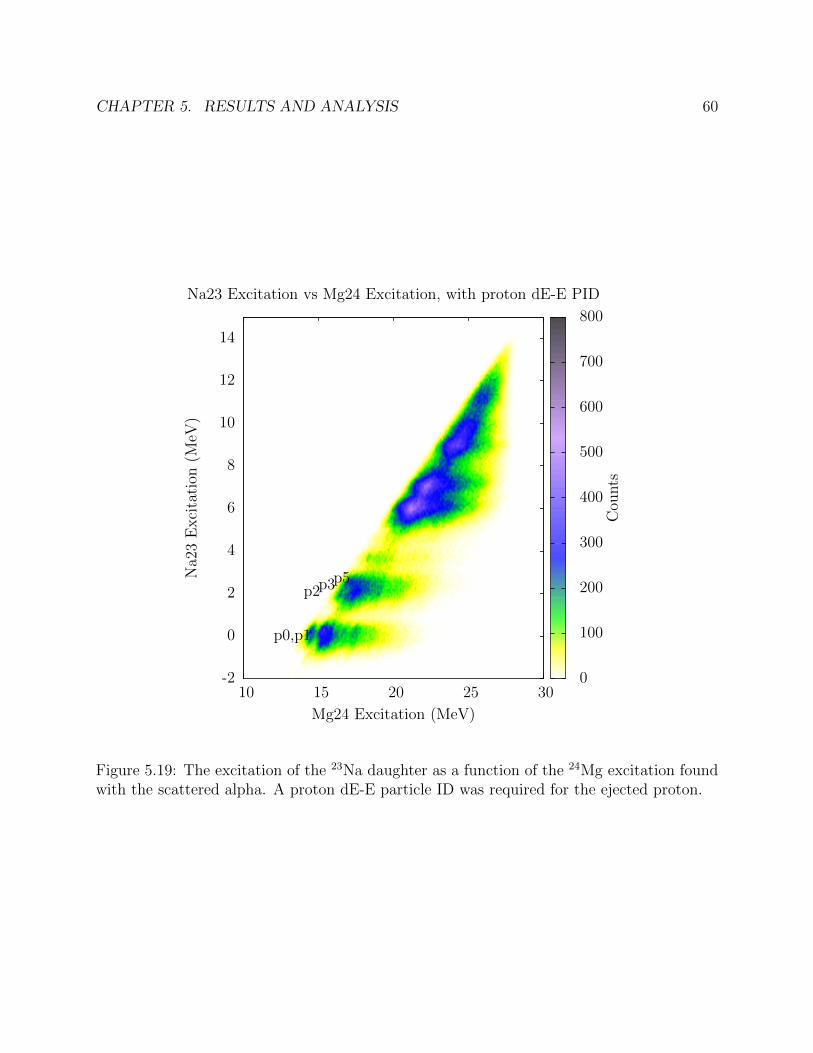
CHAPTER 5. RESULTS AND ANALYSIS 60
-2
0
2
4
6
8
10
12
14
10 15 20 25 30
Na2
3E
xci
tati
on(M
eV)
Mg24 Excitation (MeV)
Na23 Excitation vs Mg24 Excitation, with proton dE-E PID
0
100
200
300
400
500
600
700
800
Cou
nts
p0,p1
p2p3p5
Figure 5.19: The excitation of the 23Na daughter as a function of the 24Mg excitation foundwith the scattered alpha. A proton dE-E particle ID was required for the ejected proton.
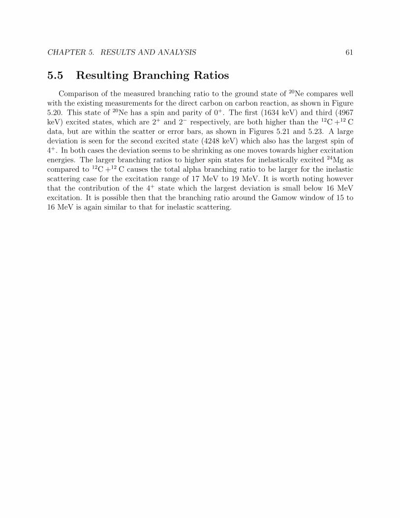
CHAPTER 5. RESULTS AND ANALYSIS 61
5.5 Resulting Branching Ratios
Comparison of the measured branching ratio to the ground state of 20Ne compares wellwith the existing measurements for the direct carbon on carbon reaction, as shown in Figure5.20. This state of 20Ne has a spin and parity of 0+. The first (1634 keV) and third (4967keV) excited states, which are 2+ and 2− respectively, are both higher than the 12C +12 Cdata, but are within the scatter or error bars, as shown in Figures 5.21 and 5.23. A largedeviation is seen for the second excited state (4248 keV) which also has the largest spin of4+. In both cases the deviation seems to be shrinking as one moves towards higher excitationenergies. The larger branching ratios to higher spin states for inelastically excited 24Mg ascompared to 12C +12 C causes the total alpha branching ratio to be larger for the inelasticscattering case for the excitation range of 17 MeV to 19 MeV. It is worth noting howeverthat the contribution of the 4+ state which the largest deviation is small below 16 MeVexcitation. It is possible then that the branching ratio around the Gamow window of 15 to16 MeV is again similar to that for inelastic scattering.
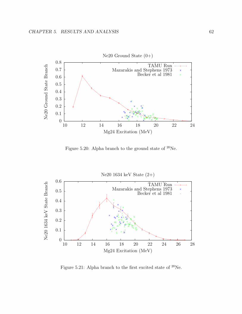
CHAPTER 5. RESULTS AND ANALYSIS 62
0
0.1
0.2
0.3
0.4
0.5
0.6
0.7
0.8
10 12 14 16 18 20 22 24
Ne2
0G
round
Sta
teB
ranch
Mg24 Excitation (MeV)
Ne20 Ground State (0+)
TAMU RunMazarakis and Stephens 1973
Becker et al 1981
Figure 5.20: Alpha branch to the ground state of 20Ne.
0
0.1
0.2
0.3
0.4
0.5
0.6
10 12 14 16 18 20 22 24 26 28
Ne2
016
34ke
VSta
teB
ranch
Mg24 Excitation (MeV)
Ne20 1634 keV State (2+)
TAMU RunMazarakis and Stephens 1973
Becker et al 1981
Figure 5.21: Alpha branch to the first excited state of 20Ne.
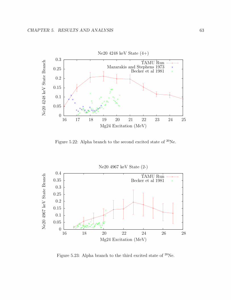
CHAPTER 5. RESULTS AND ANALYSIS 63
0
0.05
0.1
0.15
0.2
0.25
0.3
16 17 18 19 20 21 22 23 24 25
Ne2
042
48ke
VSta
teB
ranch
Mg24 Excitation (MeV)
Ne20 4248 keV State (4+)
TAMU RunMazarakis and Stephens 1973
Becker et al 1981
Figure 5.22: Alpha branch to the second excited state of 20Ne.
0
0.05
0.1
0.15
0.2
0.25
0.3
0.35
0.4
16 18 20 22 24 26 28
Ne2
049
67ke
VSta
teB
ranch
Mg24 Excitation (MeV)
Ne20 4967 keV State (2-)
TAMU RunBecker et al 1981
Figure 5.23: Alpha branch to the third excited state of 20Ne.
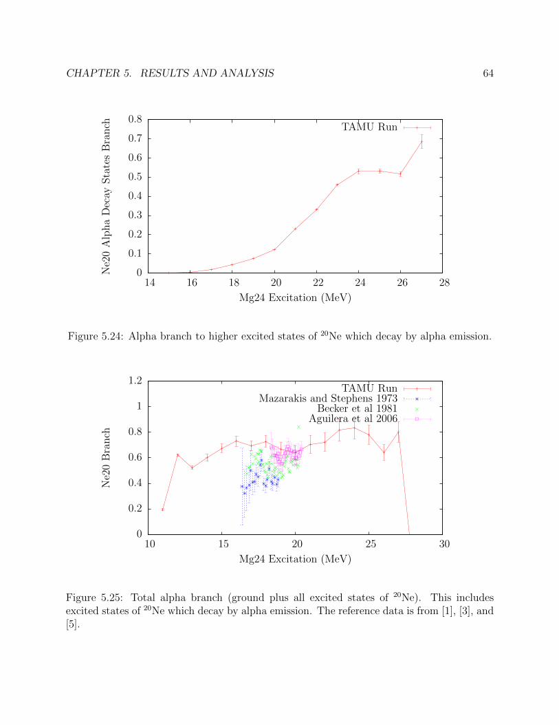
CHAPTER 5. RESULTS AND ANALYSIS 64
0
0.1
0.2
0.3
0.4
0.5
0.6
0.7
0.8
14 16 18 20 22 24 26 28
Ne2
0A
lpha
Dec
aySta
tes
Bra
nch
Mg24 Excitation (MeV)
TAMU Run
Figure 5.24: Alpha branch to higher excited states of 20Ne which decay by alpha emission.
0
0.2
0.4
0.6
0.8
1
1.2
10 15 20 25 30
Ne2
0B
ranch
Mg24 Excitation (MeV)
TAMU RunMazarakis and Stephens 1973
Becker et al 1981Aguilera et al 2006
Figure 5.25: Total alpha branch (ground plus all excited states of 20Ne). This includesexcited states of 20Ne which decay by alpha emission. The reference data is from [1], [3], and[5].
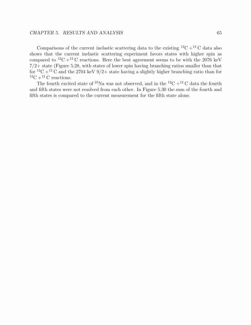
CHAPTER 5. RESULTS AND ANALYSIS 65
Comparisons of the current inelastic scattering data to the existing 12C +12 C data alsoshows that the current inelastic scattering experiment favors states with higher spin ascompared to 12C +12 C reactions. Here the best agreement seems to be with the 2076 keV7/2+ state (Figure 5.28, with states of lower spin having branching ratios smaller than thatfor 12C +12 C and the 2704 keV 9/2+ state having a slightly higher branching ratio than for12C +12 C reactions.
The fourth excited state of 23Na was not observed, and in the 12C +12 C data the fourthand fifth states were not resolved from each other. In Figure 5.30 the sum of the fourth andfifth states is compared to the current measurement for the fifth state alone.
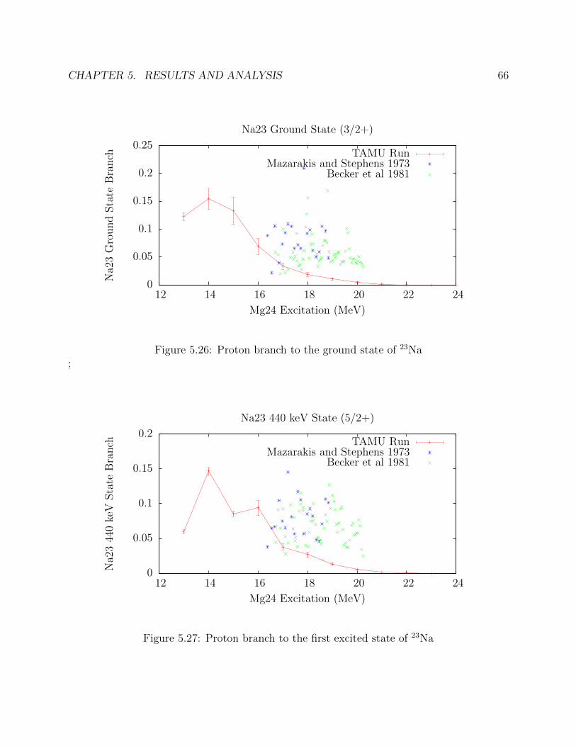
CHAPTER 5. RESULTS AND ANALYSIS 66
0
0.05
0.1
0.15
0.2
0.25
12 14 16 18 20 22 24
Na2
3G
round
Sta
teB
ranch
Mg24 Excitation (MeV)
Na23 Ground State (3/2+)
TAMU RunMazarakis and Stephens 1973
Becker et al 1981
Figure 5.26: Proton branch to the ground state of 23Na;
0
0.05
0.1
0.15
0.2
12 14 16 18 20 22 24
Na2
344
0ke
VSta
teB
ranch
Mg24 Excitation (MeV)
Na23 440 keV State (5/2+)
TAMU RunMazarakis and Stephens 1973
Becker et al 1981
Figure 5.27: Proton branch to the first excited state of 23Na
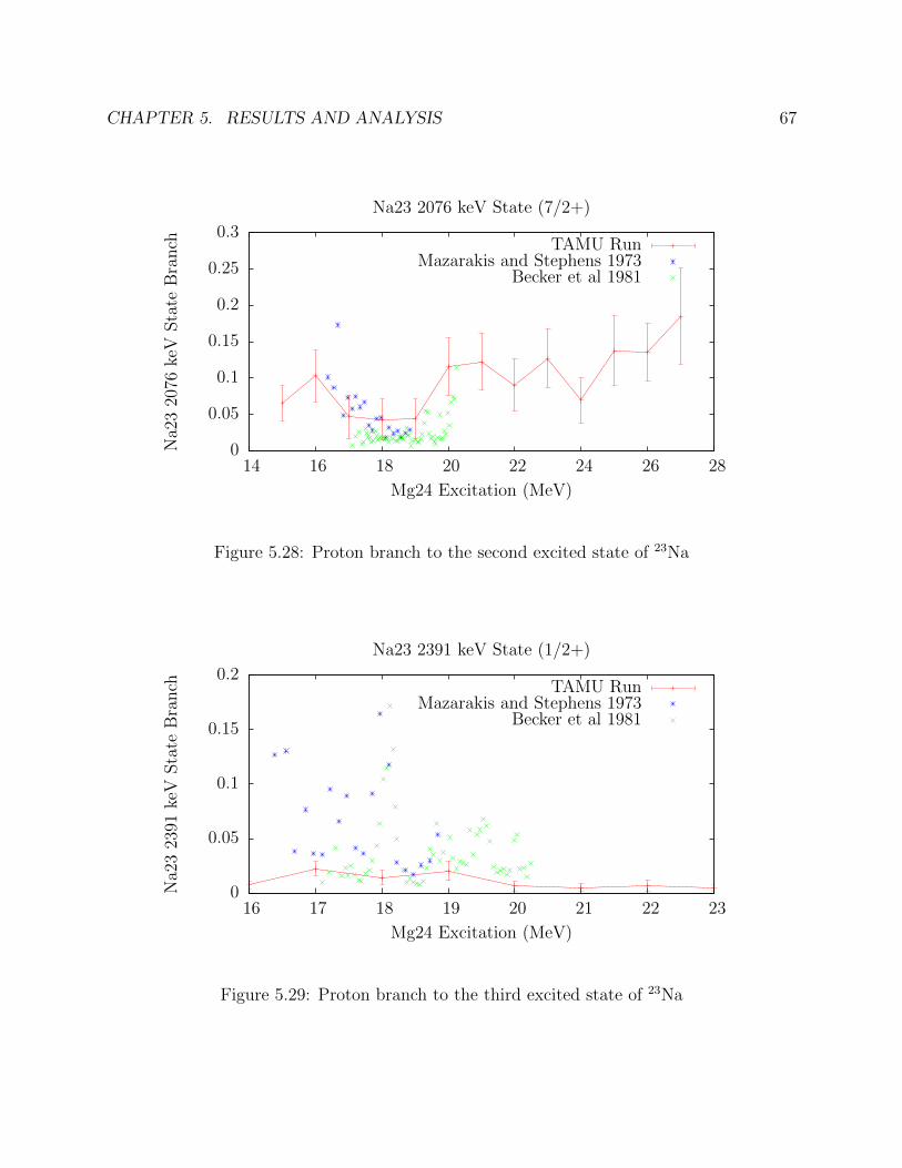
CHAPTER 5. RESULTS AND ANALYSIS 67
0
0.05
0.1
0.15
0.2
0.25
0.3
14 16 18 20 22 24 26 28
Na2
320
76ke
VSta
teB
ranch
Mg24 Excitation (MeV)
Na23 2076 keV State (7/2+)
TAMU RunMazarakis and Stephens 1973
Becker et al 1981
Figure 5.28: Proton branch to the second excited state of 23Na
0
0.05
0.1
0.15
0.2
16 17 18 19 20 21 22 23
Na2
323
91ke
VSta
teB
ranch
Mg24 Excitation (MeV)
Na23 2391 keV State (1/2+)
TAMU RunMazarakis and Stephens 1973
Becker et al 1981
Figure 5.29: Proton branch to the third excited state of 23Na
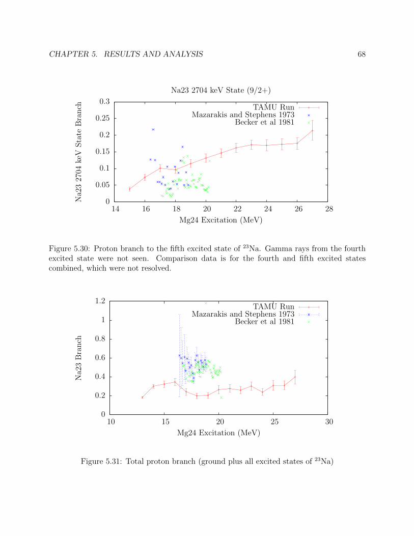
CHAPTER 5. RESULTS AND ANALYSIS 68
0
0.05
0.1
0.15
0.2
0.25
0.3
14 16 18 20 22 24 26 28
Na2
327
04ke
VSta
teB
ranch
Mg24 Excitation (MeV)
Na23 2704 keV State (9/2+)
TAMU RunMazarakis and Stephens 1973
Becker et al 1981
Figure 5.30: Proton branch to the fifth excited state of 23Na. Gamma rays from the fourthexcited state were not seen. Comparison data is for the fourth and fifth excited statescombined, which were not resolved.
0
0.2
0.4
0.6
0.8
1
1.2
10 15 20 25 30
Na2
3B
ranch
Mg24 Excitation (MeV)
TAMU RunMazarakis and Stephens 1973
Becker et al 1981
Figure 5.31: Total proton branch (ground plus all excited states of 23Na)
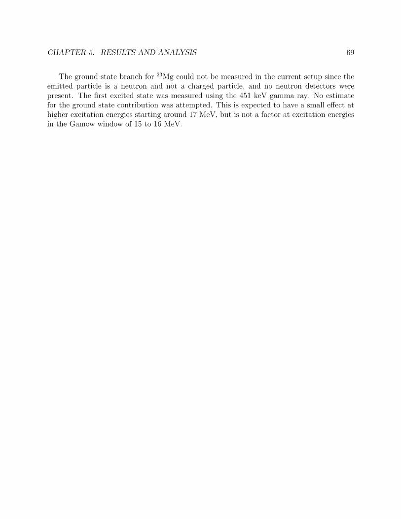
CHAPTER 5. RESULTS AND ANALYSIS 69
The ground state branch for 23Mg could not be measured in the current setup since theemitted particle is a neutron and not a charged particle, and no neutron detectors werepresent. The first excited state was measured using the 451 keV gamma ray. No estimatefor the ground state contribution was attempted. This is expected to have a small effect athigher excitation energies starting around 17 MeV, but is not a factor at excitation energiesin the Gamow window of 15 to 16 MeV.
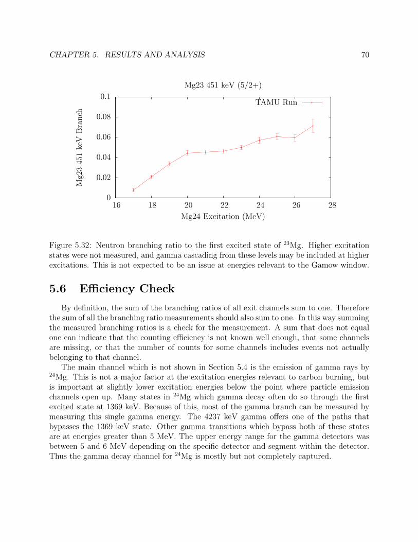
CHAPTER 5. RESULTS AND ANALYSIS 70
0
0.02
0.04
0.06
0.08
0.1
16 18 20 22 24 26 28
Mg2
345
1ke
VB
ranch
Mg24 Excitation (MeV)
Mg23 451 keV (5/2+)
TAMU Run
Figure 5.32: Neutron branching ratio to the first excited state of 23Mg. Higher excitationstates were not measured, and gamma cascading from these levels may be included at higherexcitations. This is not expected to be an issue at energies relevant to the Gamow window.
5.6 Efficiency Check
By definition, the sum of the branching ratios of all exit channels sum to one. Thereforethe sum of all the branching ratio measurements should also sum to one. In this way summingthe measured branching ratios is a check for the measurement. A sum that does not equalone can indicate that the counting efficiency is not known well enough, that some channelsare missing, or that the number of counts for some channels includes events not actuallybelonging to that channel.
The main channel which is not shown in Section 5.4 is the emission of gamma rays by24Mg. This is not a major factor at the excitation energies relevant to carbon burning, butis important at slightly lower excitation energies below the point where particle emissionchannels open up. Many states in 24Mg which gamma decay often do so through the firstexcited state at 1369 keV. Because of this, most of the gamma branch can be measured bymeasuring this single gamma energy. The 4237 keV gamma offers one of the paths thatbypasses the 1369 keV state. Other gamma transitions which bypass both of these statesare at energies greater than 5 MeV. The upper energy range for the gamma detectors wasbetween 5 and 6 MeV depending on the specific detector and segment within the detector.Thus the gamma decay channel for 24Mg is mostly but not completely captured.
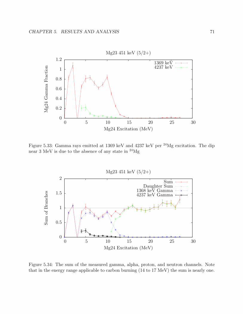
CHAPTER 5. RESULTS AND ANALYSIS 71
0
0.2
0.4
0.6
0.8
1
1.2
0 5 10 15 20 25 30
Mg2
4G
amm
aF
ract
ion
Mg24 Excitation (MeV)
Mg23 451 keV (5/2+)
1369 keV4237 keV
Figure 5.33: Gamma rays emitted at 1369 keV and 4237 keV per 24Mg excitation. The dipnear 3 MeV is due to the absence of any state in 24Mg
0
0.5
1
1.5
2
0 5 10 15 20 25 30
Sum
ofB
ranch
es
Mg24 Excitation (MeV)
Mg23 451 keV (5/2+)
SumDaughter Sum
1368 keV Gamma4237 keV Gamma
Figure 5.34: The sum of the measured gamma, alpha, proton, and neutron channels. Notethat in the energy range applicable to carbon burning (14 to 17 MeV) the sum is nearly one.
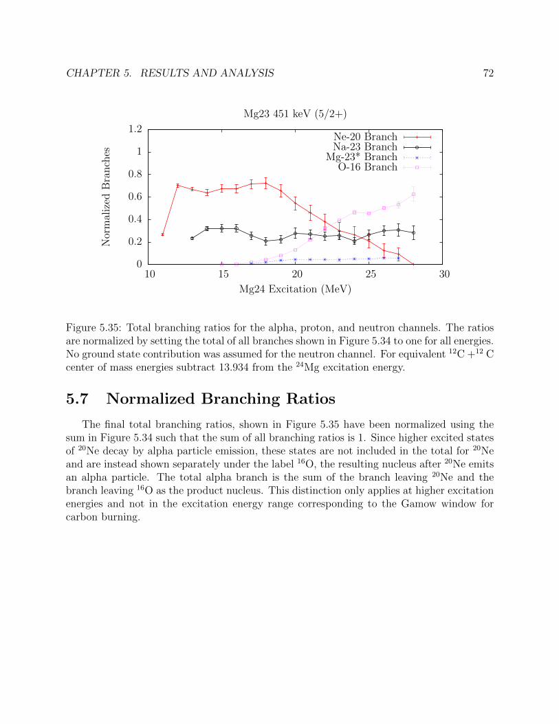
CHAPTER 5. RESULTS AND ANALYSIS 72
0
0.2
0.4
0.6
0.8
1
1.2
10 15 20 25 30
Nor
mal
ized
Bra
nch
es
Mg24 Excitation (MeV)
Mg23 451 keV (5/2+)
Ne-20 BranchNa-23 Branch
Mg-23* BranchO-16 Branch
Figure 5.35: Total branching ratios for the alpha, proton, and neutron channels. The ratiosare normalized by setting the total of all branches shown in Figure 5.34 to one for all energies.No ground state contribution was assumed for the neutron channel. For equivalent 12C +12 Ccenter of mass energies subtract 13.934 from the 24Mg excitation energy.
5.7 Normalized Branching Ratios
The final total branching ratios, shown in Figure 5.35 have been normalized using thesum in Figure 5.34 such that the sum of all branching ratios is 1. Since higher excited statesof 20Ne decay by alpha particle emission, these states are not included in the total for 20Neand are instead shown separately under the label 16O, the resulting nucleus after 20Ne emitsan alpha particle. The total alpha branch is the sum of the branch leaving 20Ne and thebranch leaving 16O as the product nucleus. This distinction only applies at higher excitationenergies and not in the excitation energy range corresponding to the Gamow window forcarbon burning.
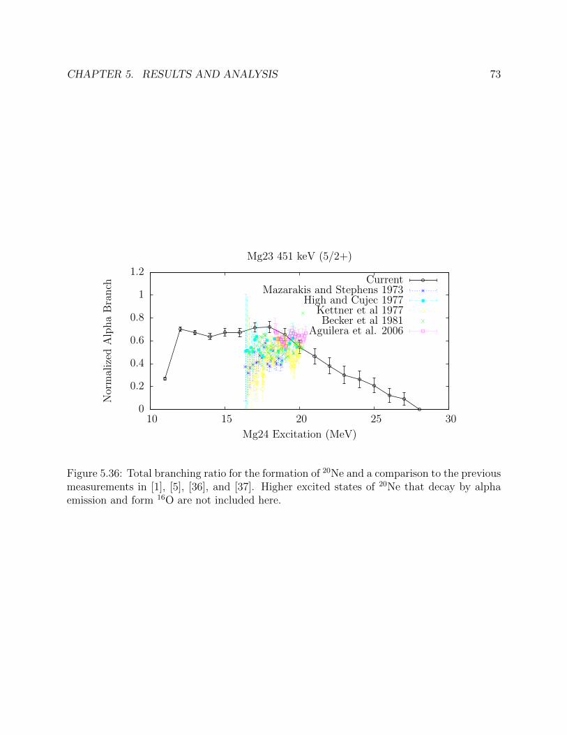
CHAPTER 5. RESULTS AND ANALYSIS 73
0
0.2
0.4
0.6
0.8
1
1.2
10 15 20 25 30
Nor
mal
ized
Alp
ha
Bra
nch
Mg24 Excitation (MeV)
Mg23 451 keV (5/2+)
CurrentMazarakis and Stephens 1973
High and Cujec 1977Kettner et al 1977Becker et al 1981
Aguilera et al. 2006
Figure 5.36: Total branching ratio for the formation of 20Ne and a comparison to the previousmeasurements in [1], [5], [36], and [37]. Higher excited states of 20Ne that decay by alphaemission and form 16O are not included here.
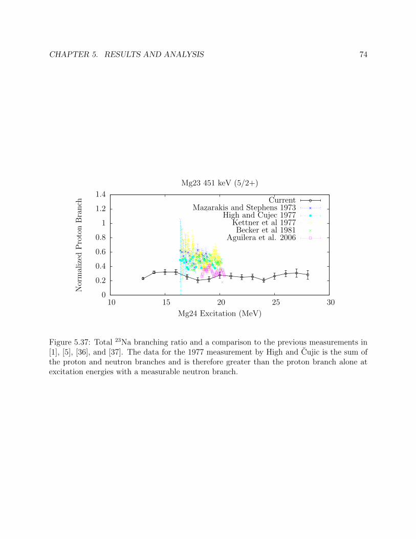
CHAPTER 5. RESULTS AND ANALYSIS 74
0
0.2
0.4
0.6
0.8
1
1.2
1.4
10 15 20 25 30
Nor
mal
ized
Pro
ton
Bra
nch
Mg24 Excitation (MeV)
Mg23 451 keV (5/2+)
CurrentMazarakis and Stephens 1973
High and Cujec 1977Kettner et al 1977Becker et al 1981
Aguilera et al. 2006
Figure 5.37: Total 23Na branching ratio and a comparison to the previous measurements in[1], [5], [36], and [37]. The data for the 1977 measurement by High and Cujic is the sum ofthe proton and neutron branches and is therefore greater than the proton branch alone atexcitation energies with a measurable neutron branch.
75
Chapter 6
Conclusion
Measurements of the branching ratios for the decay of 24Mg excited by the inelasticscattering of 40 MeV alpha particles have been made. The range of excitation energiesstudied extends to 27 MeV. This range includes the excitation energies present in the 24Mgcompound nucleus formed in carbon burning reactions, which have excitation energies in therange of 15 to 16 MeV. This experiment was selected as a possible surrogate measurementfor the branching ratios for the carbon burning compound nucleus, and consequently theratios of the cross sections for the reactions 12C +12 C→20 Ne + α, 12C +12 C→23 Na + p,and 12C +12 C→23 Mg + n.
The angular distribution of the scattered alpha particles leading to 24Mg excitation en-ergies similar to those present in a carbon burning reaction compound nucleus show somepreference for smaller angles in the region of 0.4 to 0.8 radians. A fully compound re-action mechanism for inelastic scattering would produce an angular cross section that isapproximately isotropic. This indicates that the scattering mechanism is not only that of acompound reaction. Scattering in a compound reaction would leave the nucleus in a statethat is similar to the compound nucleus in a carbon burning reaction but this does not ruleout the possibility that a nucleus excited by a different mechanism would evolve into a statesimilar to that of a carbon burning compound nucleus.
A related issue is that of the angular momentum distribution of the inelastically excited24Mg as compared to the 24Mg compound nucleus in carbon burning. Inelastic scattering of40 MeV alpha particles has the potential to bring in higher amounts of angular momentumthan expected for the carbon burning compound nucleus. If the Weisskopf-Ewing limitholds for this system then the difference in the angular momentum distributions will notaffect the branching ratios, but this assumption must be supported by comparisons to datataken from direct carbon on carbon experiments. These comparisons show that at leastfor certain ranges of excitation energy that inelastic scattering of 40 MeV alpha particlesproduces a distribution of excited 24Mg that favors decays into higher spin states of 20Ne and23Na relative to the excited 24Mg created as the compound nucleus in carbon burning. Thisindicates that this system does not fully meet the criteria for the Weisskopf-Ewing limit. It
CHAPTER 6. CONCLUSION 76
also suggests that the average spin distribution in the inelastically excited 24Mg is higherthan that of the 24Mg compound nucleus in carbon burning.
While these differences prevent assigning a direct equality between the branching ratiosfound with inelastic scattering and in carbon burning, the branching ratios found in theinelastic scattering case do appear to have a relation to those in carbon burning which mightallow an estimate of the branching ratios for carbon burning to be made in the region of theGamow window. The branching ratios to some states of 20Ne and 23Na were very similarfor the inelastic scattering case and the carbon burning case. Additionally, as the excitationenergy is decreased to the range of the Gamow window many of the branching ratios to thehigher excited states diminish, reducing the total number of states which must be understoodin order to predict the branching ratio.
77
Bibliography
[1] M. G. Mazarakis and W. E. Stephens. Experimental measurements of the 12C +12 Cnuclear reactions at low energies. Physical Review C, 7(4):1280–1287, 1973.
[2] R. Dayras, Z. E. Switkowski, and S. E. Woosley. Neutron branching in the reaction 12c+ 12c. Nuclear Physics A, 279(1):70–84, 1977.
[3] H.W. Becker, K.U. Kettner, C. Rolfs, and H.P. Trautvetter. The12c+12c reaction atsubcoulomb energies (ii). Zeitschrift fA¼r Physik A Atoms and Nuclei, 303(4):305–312,1981.
[4] L. Barron-Palos, E. Chavez L., A. Huerta H., M. Ortiz, G. Murillo O., E. Aguilera R.,E. Martınez Q., E. Moreno, R. Policroniades R., and A. Varela G. 12C +12 C cross-section measurements at low energies. The European Physical Journal A - Hadrons andNuclei, 25:645–646, 2005. 10.1140/epjad/i2005-06-008-2.
[5] E. F. Aguilera, P. Rosales, E. Martinez-Quiroz, G. Murillo, M. Fernandez, H. Berdejo,D. Lizcano, A. Gomez-Camacho, R. Policroniades, A. Varela, E. Moreno, E. Chavez,M. E. Ortız, A. Huerta, T. Belyaeva, and M. Wiescher. New [gamma]-ray measurementsfor 12c + 12c sub-coulomb fusion: Toward data unification. Physical Review C, 73:064601,2006.
[6] L. Barron-Palos, E.F. Aguilera, J. Aspiazu, A. Huerta, E. Martınez-Quiroz, R. Monroy,E. Moreno, G. Murillo, M.E. Ortiz, R. Policroniades, A. Varela, and E. Chavez. Absolutecross sections measurement for the 12c + 12c system at astrophysically relevant energies.Nuclear Physics A, 779:318–332, 2006.
[7] T. Spillane, F. Raiola, C. Rolfs, D. Schurmann, F. Strieder, S. Zeng, H.-W. Becker,C. Bordeanu, L. Gialanella, M. Romano, and J. Schweitzer. 12C +12 C fusion reactionsnear the gamow energy. Physical Review Letters, 98:122501, 2007.
[8] Claus E. Rolfs and William S. Rodney. Cauldrons in the Cosmos. The University ofChicago Press, Chicago 60637, 1988.
[9] C. J. Hansen and S. D. Kawaler. Stellar Interiors: Physical Principles, Structure, andEvolution. Springer-Verlag New York, Inc., 1994.
BIBLIOGRAPHY 78
[10] Q value calculator. http://www.nndc.bnl.gov/qcalc/. Accessed: 2015-04-19.
[11] Jutta E. Escher, Frank S. Dietrich, and Christian Forssen. Surrogate nuclear reactionmethods for astrophysics. Nuclear Instruments and Methods in Physics Research Sec-tion B: Beam Interactions with Materials and Atoms, 261(1-2):1075–1078, 2007. TheApplication of Accelerators in Research and Industry - Proceedings of the NineteenthInternational Conference on The Application of Accelerators in Research and Industry,Nineteenth International Conference on The Application of Accelerators in Researchand Industry.
[12] K. Lundmark. Svenska Vetenkapsakad. Handl., 60:8, 1920.
[13] Wolfgang Hillebrandt and Jens C. Niemeyer. Type ia supernova explosion models.Annual Review of Astronomy and Astrophysics, 38:191 – 230, 2000.
[14] W. Baade and F. Zwicky. Remarks on super-novae and cosmic rays. Phys. Rev.,46(1):76–77, Jul 1934.
[15] R. Minkowski. Publ. Astron. Soc. Pac., 52:206, 1940.
[16] J. C. Wheeler and R. P. Harkness. Rep. Prog. Phys., 53:1467–557, 1990.
[17] F. Hoyle and W. A. Fowler. Nucleosynthesis in supernovae. Astrophysical Journal,132:565–590, 1960.
[18] J. W. Truran, D. Arnett, and A. G. W. Cameron. Canad. J. Physics, 45:2315–32, 1967.
[19] S. A. Colgate and C. McKee. Astrophysical Journal, 157:623, 1969.
[20] F. Zwicky. On the theory and observation of highly collapsed stars. Phys. Rev.,55(8):726–743, Apr 1939.
[21] O. C. Wilson. Astrophysical Journal, 90:634, 1939.
[22] F. Hoyle. The synthesis of elements from hydrogen. M. N. R. A. S., 106:343 – 383,1946.
[23] C. Marty. Generalized optical theorem and integrated cross-sections. Zeitschrift furPhysik A Hadrons and Nuclei, 309:261–265, 1983. 10.1007/BF01413758.
[24] R. and Lipperheide. Heavy-ion reaction cross sections from elastic scattering data.Nuclear Physics A, 469(1):190–204, 1987.
[25] A. N. Ostrowski, T. Davinson, K. Fohl, M. Seidl, and H. Voit. Carbon-burning: Totalreaction cross section at ec.m.=2.5-1.6 mev. Nuclear Physics A, 688(1-2):130–133, 2001.

BIBLIOGRAPHY 79
[26] C. L. Jiang, K. E. Rehm, B. B. Back, and R. V. F. Janssens. Expectations for 12C and16O induced fusion cross sections at energies of astrophysical interest. Physical ReviewC, 75:015803, 2007.
[27] R. Bass. Fusion of heavy nuclei in a classical model. Nuclear Physics A, 231:45 – 63,1974.
[28] R. Bass. Nucleus-nucleus potential deduced from experimental fusion cross sections.Physical Review Letters, 39(5):265 – 268, 1977.
[29] Nndc website. http://www.nndc.bnl.gov/. Accessed: 2015-06-15.
[30] Frank S. Dietrich. Simple derivation of the hauser-feshbach and weisskoph-ewing for-mulae, with application to surrogate reactions ucrl-tr-201718.
[31] Jutta E. Escher and Frank S. Dietrich. Determining (n, f) cross sections for actinidenuclei indirectly: Examination of the surrogate ratio method. Phys. Rev. C, 74:054601,Nov 2006.
[32] A. J. Koning, S. Hilaire, and M. C. Duijvestijn. Talys-1.0. Proceedings of the Interna-tional Conference on Nuclear Data for Science and Technology - ND2007, pages 211 –214, 2007.
[33] S.R. Lesher, L. Phair, L.A. Bernstein, D.L. Bleuel, J.T. Burke, J.A. Church, P. Fallon,J. Gibelin, N.D. Scielzo, and M. Wiedeking. Stars/liberace: Segmented silicon andhigh-purity germanium detector arrays for low-energy nuclear reaction and structurestudies. Nuclear Instruments and Methods in Physics Research Section A: Accelerators,Spectrometers, Detectors and Associated Equipment, 621(1a€“3):286 – 291, 2010.
[34] M. Pignanelli, S. Micheletti, R. De Leo, S. Brandenburg, and M. N. Harakeh. Nuclearmatter density effects in monopole transitions. Phys. Rev. C, 33:40–49, Jan 1986.
[35] Kenneth S. Krane. Introductory Nuclear Physics. John Wiley & Sons, Inc., 1988.
[36] M.D. High and B. AŒujec. The 12c + 12c sub-coulomb fusion cross section. NuclearPhysics A, 282(1):181 – 188, 1977.
[37] K. U. Kettner, H. Lorenz-Wirzba, C. Rolfs, and H. Winkler. Study of the fusion reaction12C + 12C below the coulomb barrier. Phys. Rev. Lett., 38:337–340, Feb 1977.