Digital image processingusing Matlab

School of Mechanical Engineering

Pusan National University

Kim Dong Woon

dongwoonkim@pusan.ac.kr

051-510-3921

통합기계관 120호

Digital image processing

• 디지털 화상처리 또는 디지털 영상 처리는 컴퓨터 알고리즘을 사용하여

디지털 이미지에 대한 화상처리를 수행하는 것이다.

• 디지털 영상 처리는 영상 처리를 위한 훨씬 더 복잡한 알고리즘 사용을 가

능하게 하므로, 단순작업에 더욱 정교한 성능과 아날로그 수단으로는 불가

능한 방법의 실행, 양쪽을 가능하게 한다.

영상을 높은 질의 영상으로 변환 (Image Enhancement)

변질된 영상을 복원 (Image Restoration)

영상내의 특징을 추출, 사용 (Image Understanding)

영상의 일부분으로부터 새로운 영상을 생성 (New Image Creation)

영상 압축 (Image Abstraction / Compression)

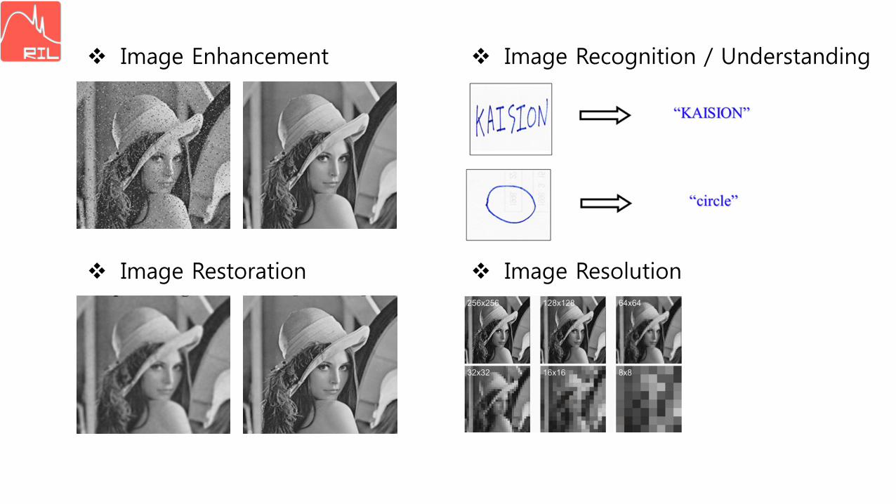
Image Enhancement

Image Restoration

Image Recognition / Understanding

Image Resolution

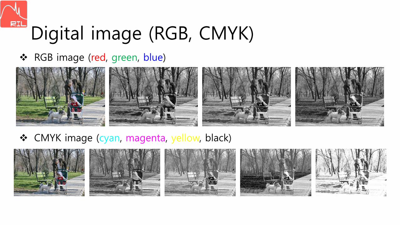
Digital image (RGB, CMYK) RGB image (red, green, blue)

CMYK image (cyan, magenta, yellow, black)

ImageJ

• http://imagej.nih.gov/ij/

• Google -> ImageJ 검색

• ImageJ is an open sourceprocessing program designedfor scientific multidimensionalimages

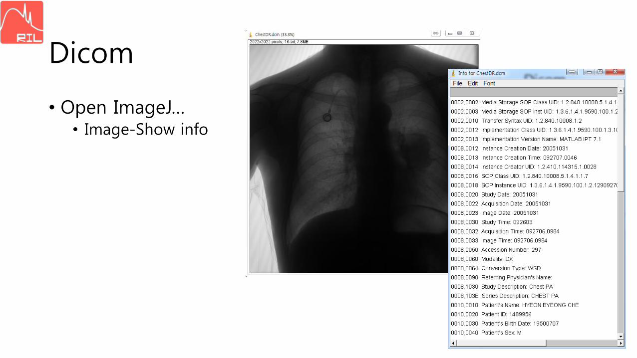
Dicom

• Open ImageJ…• Image-Show info

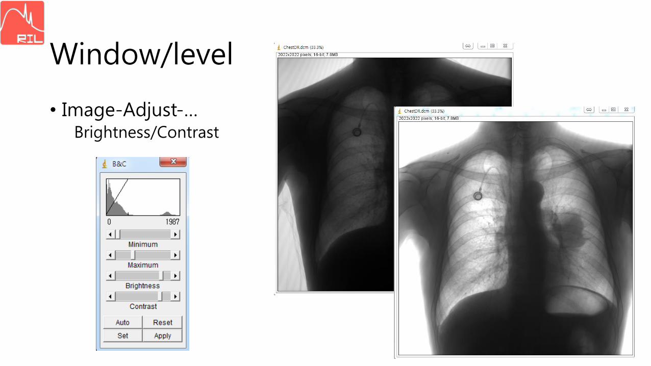
Window/level

• Image-Adjust-…Brightness/Contrast

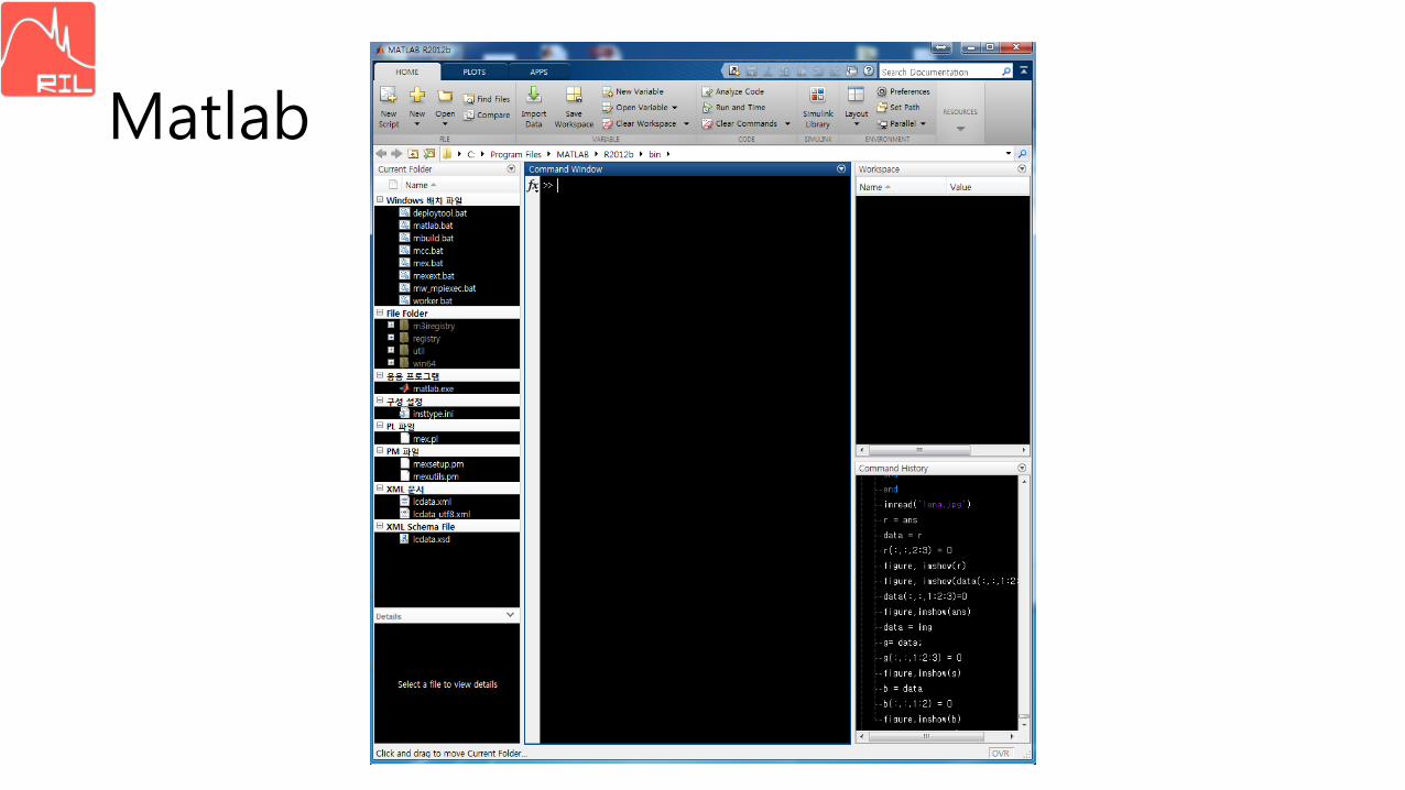
Matlab

Matlab

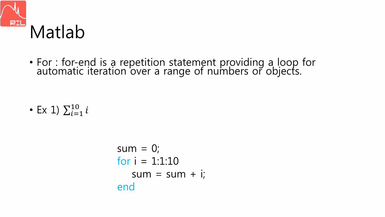
• For : for-end is a repetition statement providing a loop for automatic iteration over a range of numbers or objects.

• Ex 1) σ𝑖=110 𝑖

sum = 0;for i = 1:1:10

sum = sum + i;end

Matlab

• Ex 2) sum(1:10), odd number

Sum = 0;

for i=1:1:10

if mod(i,2)==1

Sum = Sum+i;

end

end

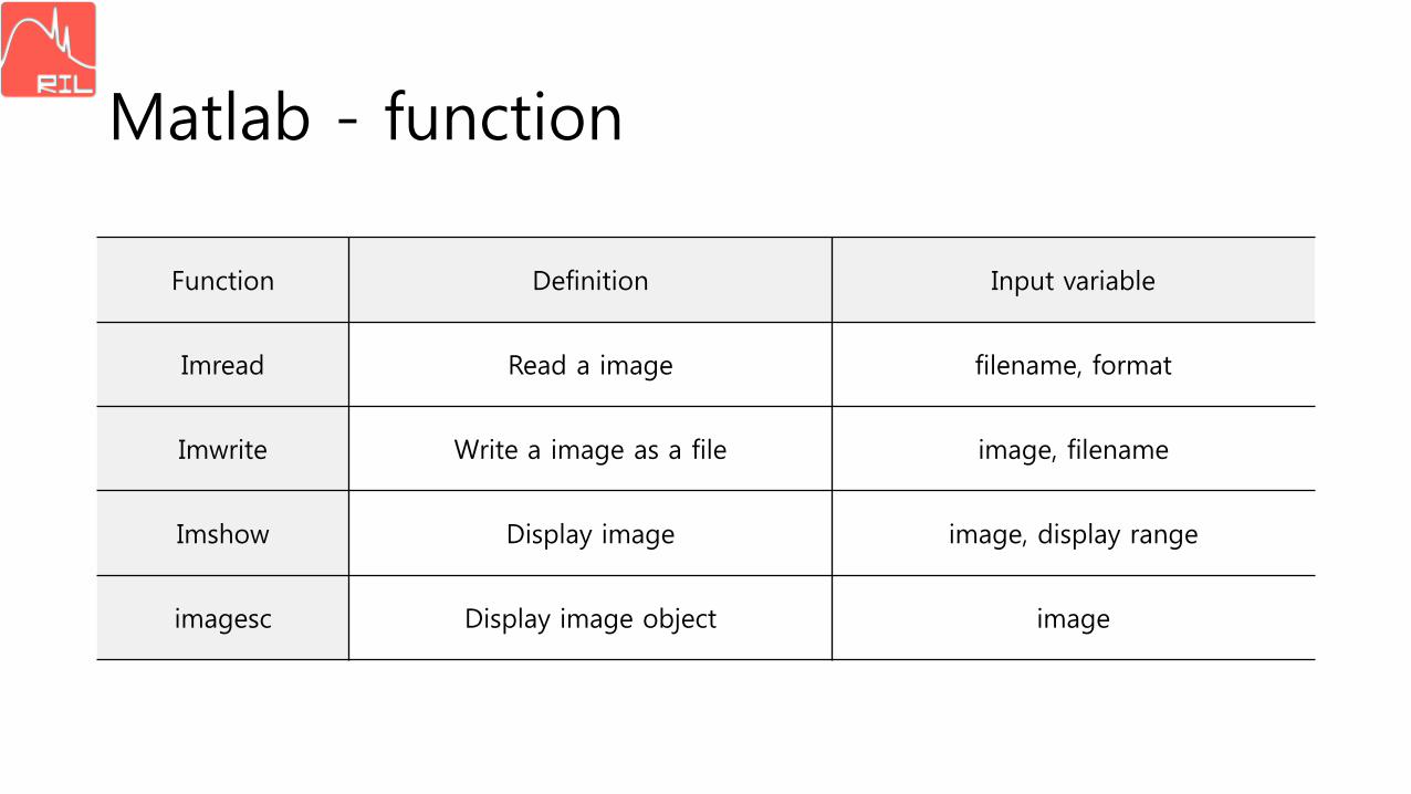
Matlab - function

Function Definition Input variable

Imread Read a image filename, format

Imwrite Write a image as a file image, filename

Imshow Display image image, display range

imagesc Display image object image

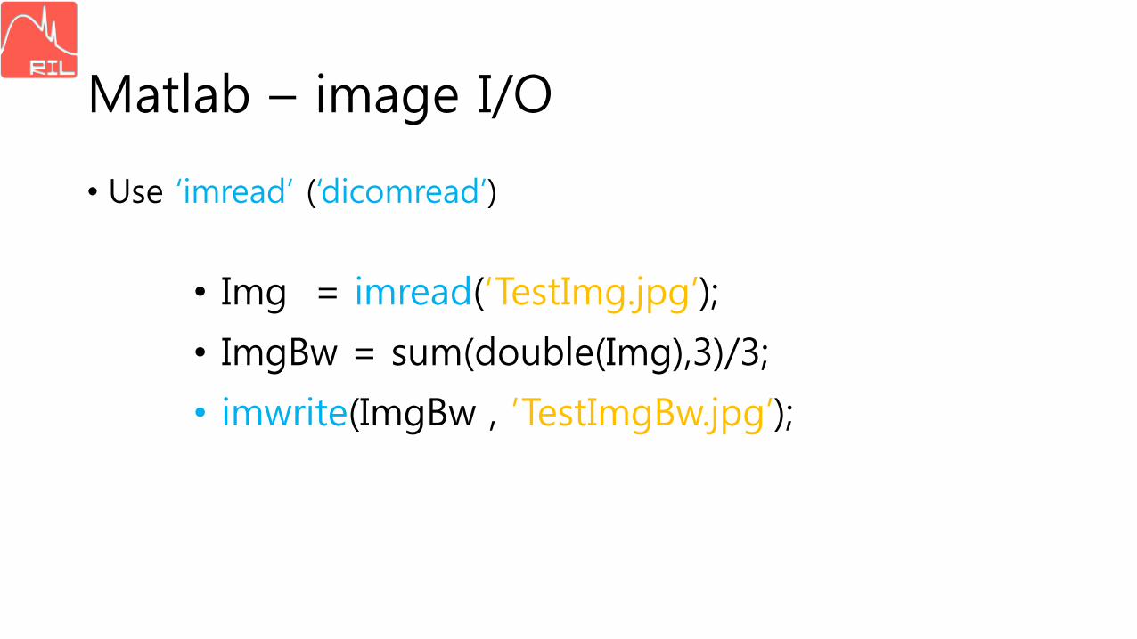
Matlab – image I/O

• Use ‘imread’ (‘dicomread’)

• Img = imread(‘TestImg.jpg’);

• ImgBw = sum(double(Img),3)/3;

• imwrite(ImgBw , ’TestImgBw.jpg’);

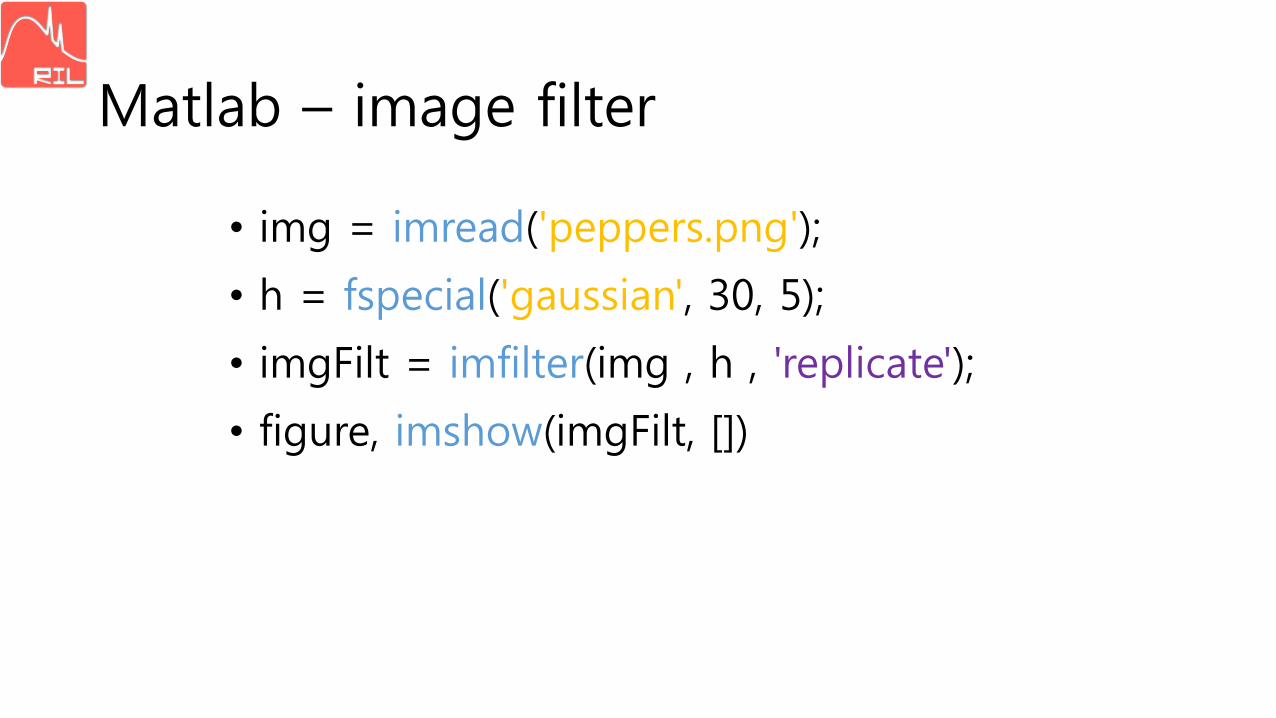
Matlab – image filter

• img = imread('peppers.png');

• h = fspecial('gaussian', 30, 5);

• imgFilt = imfilter(img , h , 'replicate');

• figure, imshow(imgFilt, [])

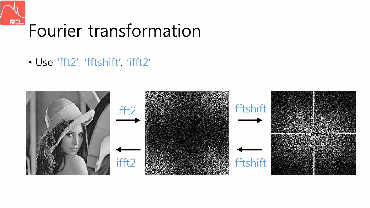
Fourier transformation

• Use ‘fft2’, ‘fftshift’, ‘ifft2’

fft2 fftshift

ifft2 fftshift

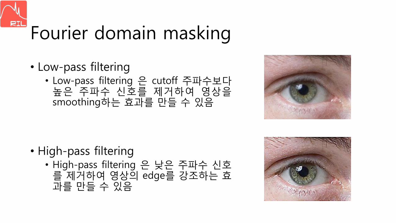
Fourier domain masking

• Low-pass filtering• Low-pass filtering 은 cutoff 주파수보다높은 주파수 신호를 제거하여 영상을smoothing하는 효과를 만들 수 있음

• High-pass filtering• High-pass filtering 은 낮은 주파수 신호를 제거하여 영상의 edge를 강조하는 효과를 만들 수 있음

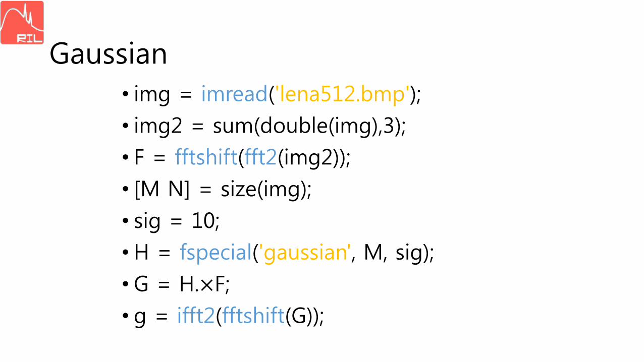
Gaussian

• img = imread('lena512.bmp');

• img2 = sum(double(img),3);

• F = fftshift(fft2(img2));

• [M N] = size(img);

• sig = 10;

•H = fspecial('gaussian', M, sig);

• G = H.×F;

• g = ifft2(fftshift(G));

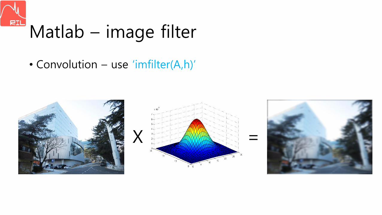
Matlab – image filter

• Convolution – use ‘imfilter(A,h)’

X =

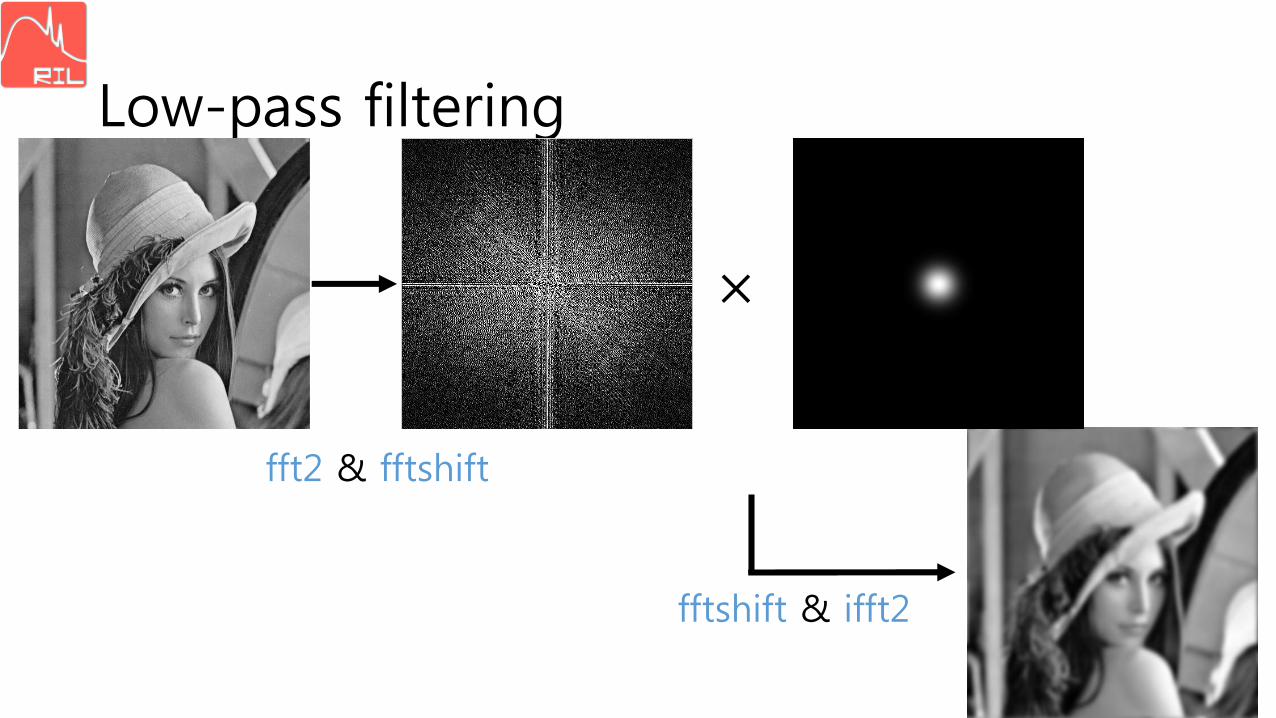
Low-pass filtering

fft2 & fftshift

×

fftshift & ifft2

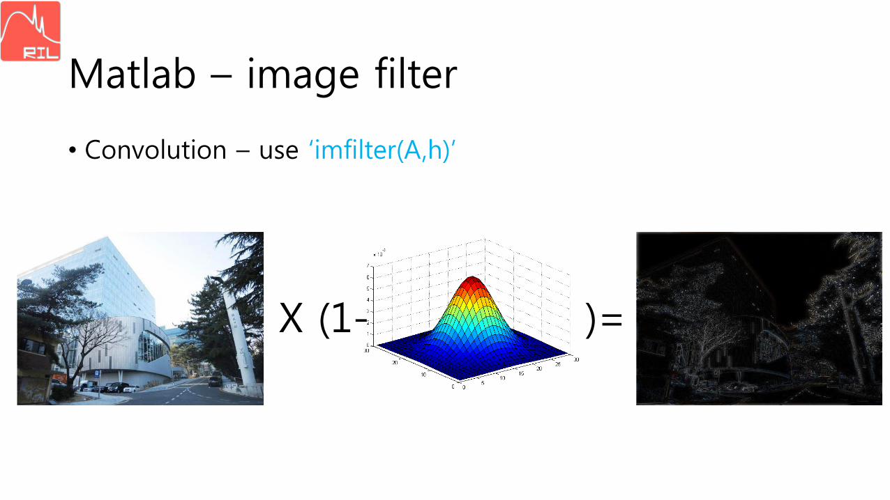
Matlab – image filter

• Convolution – use ‘imfilter(A,h)’

X (1- )=

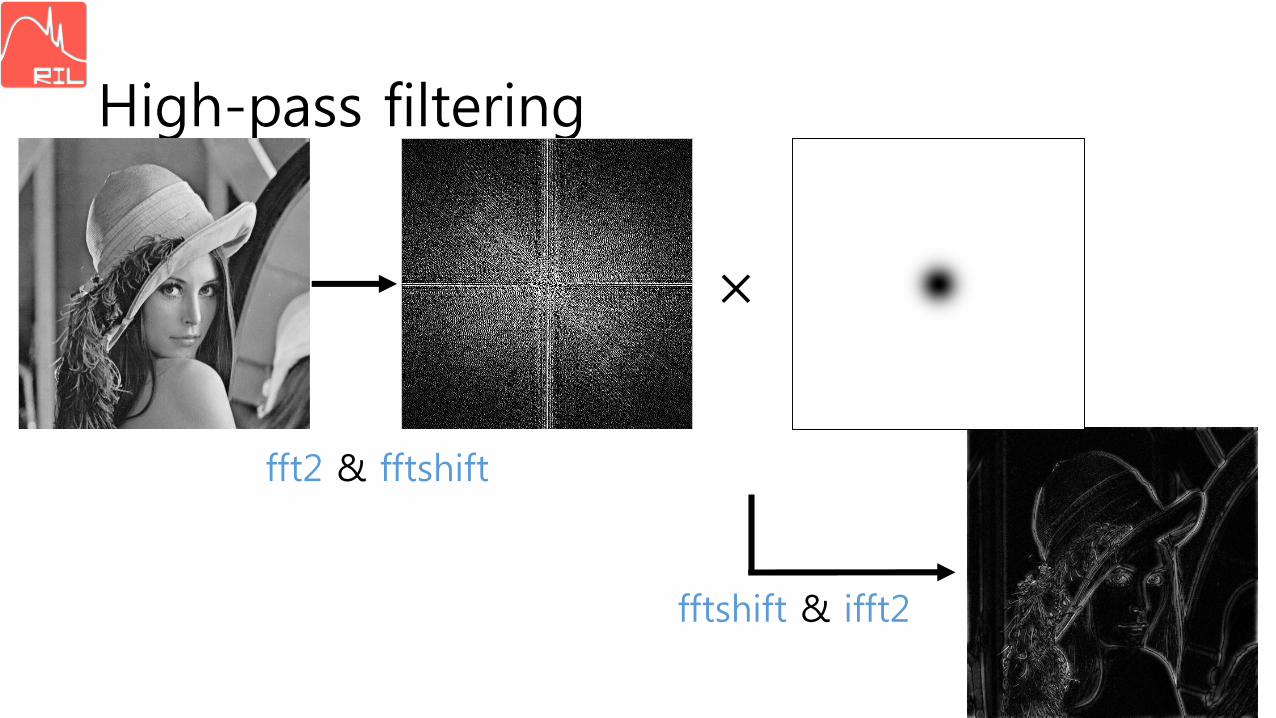
High-pass filtering

fft2 & fftshift

×

fftshift & ifft2

Matlab – image filter

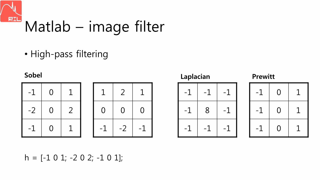
• High-pass filtering

-1 0 1

-2 0 2

-1 0 1

1 2 1

0 0 0

-1 -2 -1

-1 -1 -1

-1 8 -1

-1 -1 -1

-1 0 1

-1 0 1

-1 0 1

Sobel Laplacian Prewitt

h = [-1 0 1; -2 0 2; -1 0 1];

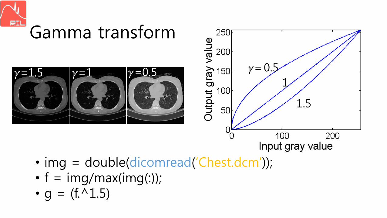
Gamma transform

0.5

1

1.5

𝛾=𝛾=1.5 𝛾=1 𝛾=0.5

• img = double(dicomread(‘Chest.dcm'));• f = img/max(img(:));• g = (f.^1.5)

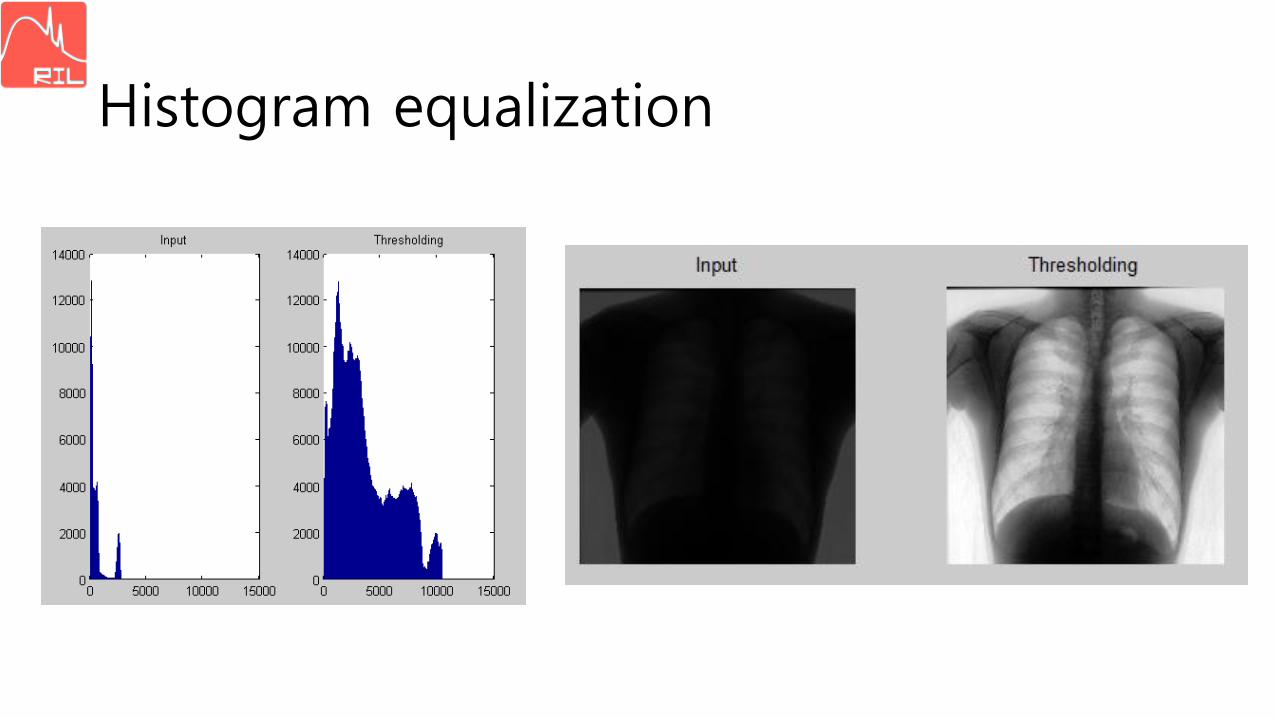
Histogram equalization

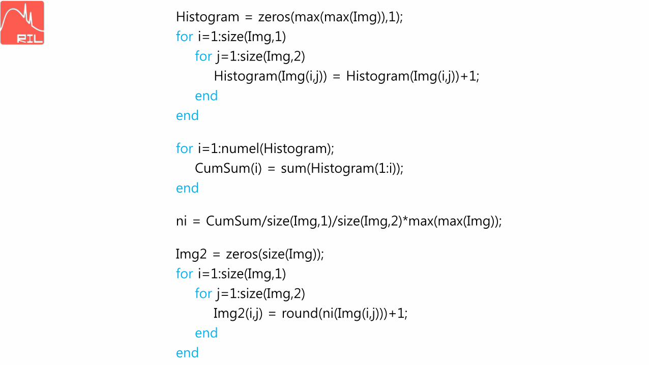
Histogram = zeros(max(max(Img)),1);

for i=1:size(Img,1)

for j=1:size(Img,2)

Histogram(Img(i,j)) = Histogram(Img(i,j))+1;

end

end

for i=1:numel(Histogram);

CumSum(i) = sum(Histogram(1:i));

end

ni = CumSum/size(Img,1)/size(Img,2)*max(max(Img));

Img2 = zeros(size(Img));

for i=1:size(Img,1)

for j=1:size(Img,2)

Img2(i,j) = round(ni(Img(i,j)))+1;

end

end

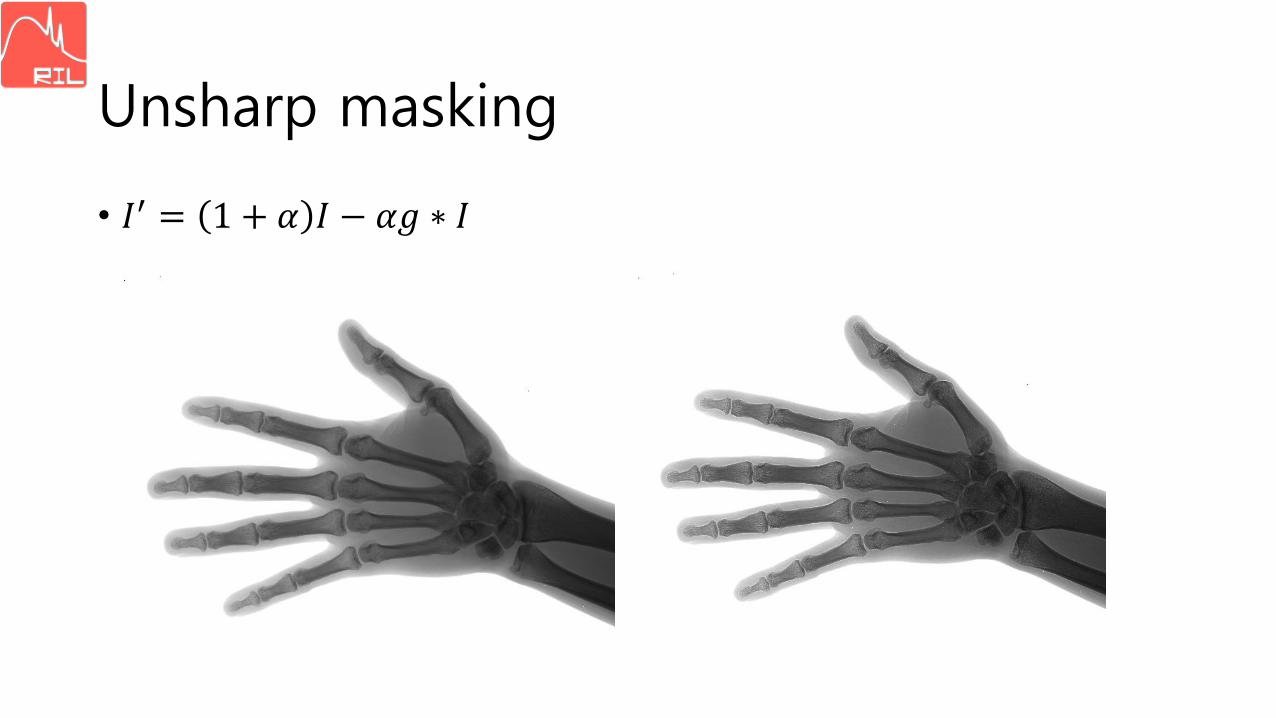
Unsharp masking

• 𝐼′ = 1 + 𝛼 𝐼 − 𝛼𝑔 ∗ 𝐼

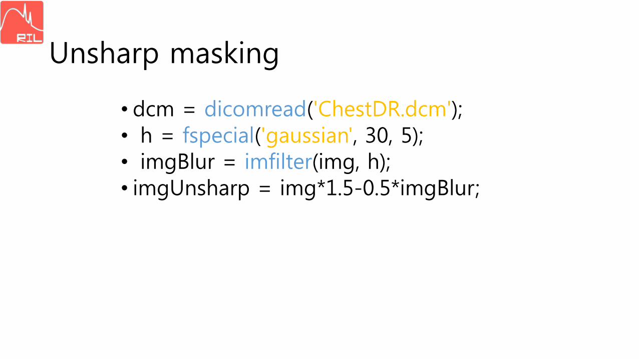
Unsharp masking

• dcm = dicomread('ChestDR.dcm');• h = fspecial('gaussian', 30, 5);• imgBlur = imfilter(img, h);• imgUnsharp = img*1.5-0.5*imgBlur;

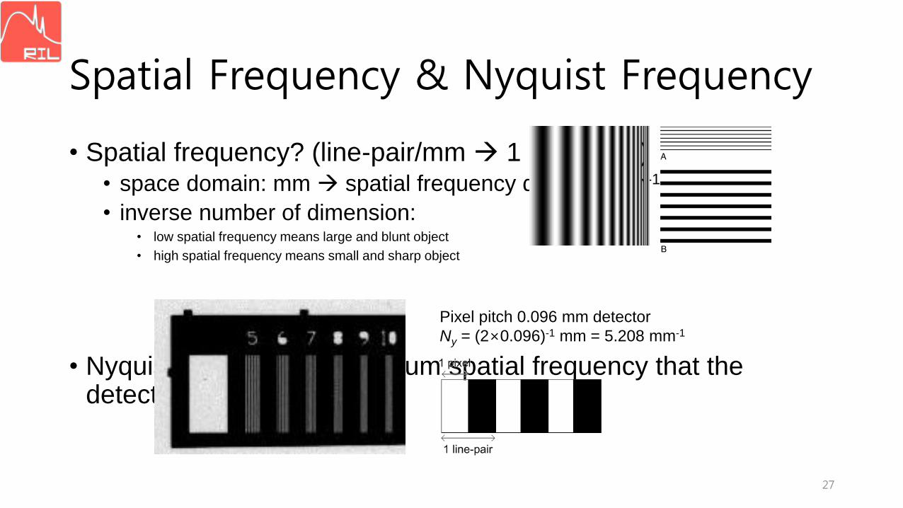
Spatial Frequency & Nyquist Frequency

• Spatial frequency? (line-pair/mm 1 cycle/mm)• space domain: mm spatial frequency domain: mm-1

• inverse number of dimension: • low spatial frequency means large and blunt object

• high spatial frequency means small and sharp object

• Nyquist frequency = maximum spatial frequency that the detector can distinguish

27

Pixel pitch 0.096 mm detector

Ny = (2×0.096)-1 mm = 5.208 mm-1

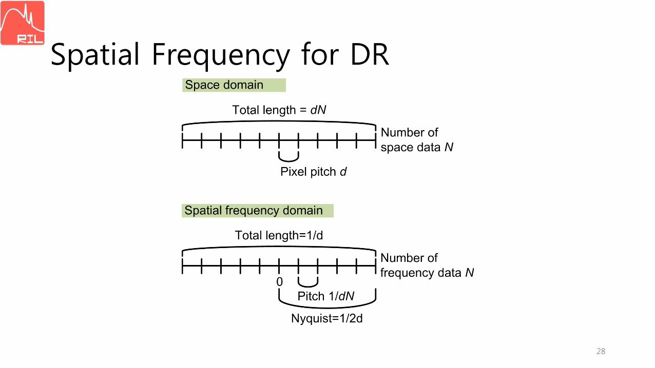
Spatial Frequency for DR

28

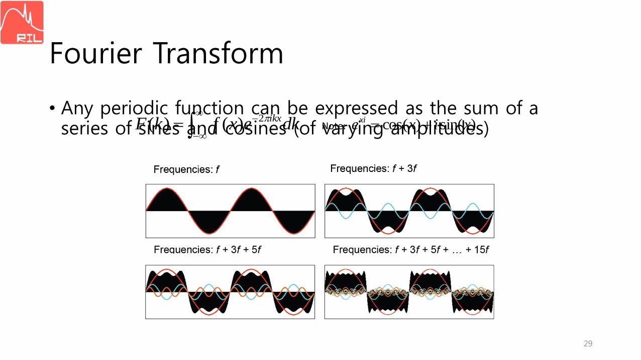
Fourier Transform

• Any periodic function can be expressed as the sum of a series of sines and cosines (of varying amplitudes)

29

dkexfkF ikx2)()( )sin()cos( xixexi Note:

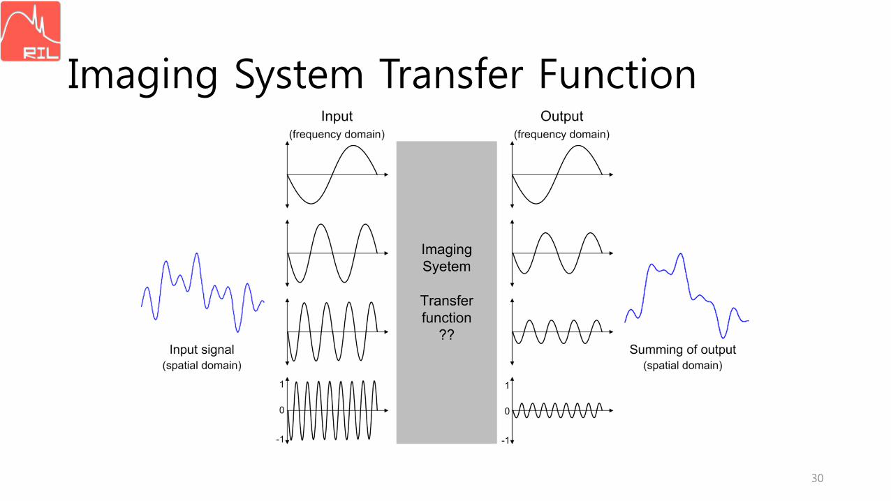
Imaging System Transfer Function

30

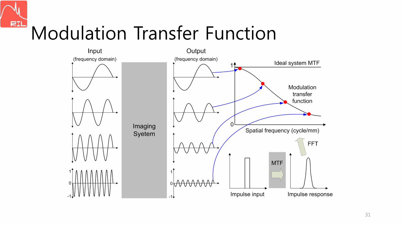
Modulation Transfer Function

31

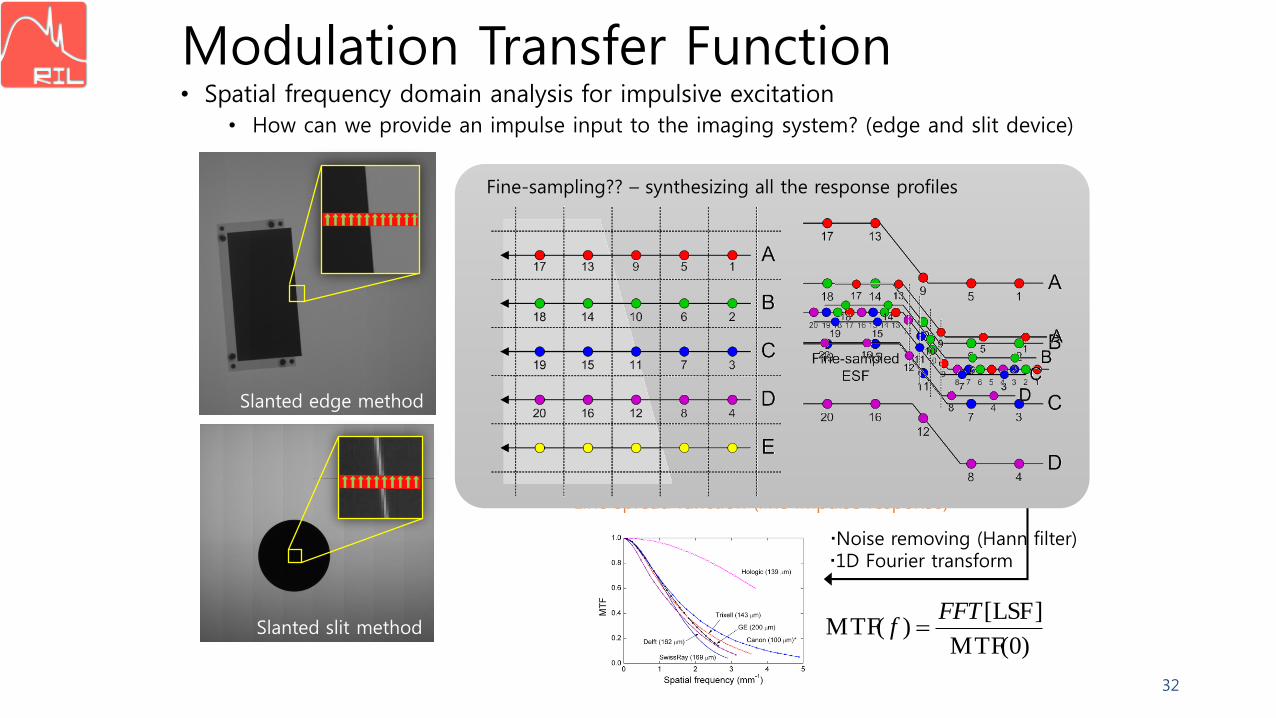
• Spatial frequency domain analysis for impulsive excitation

• How can we provide an impulse input to the imaging system? (edge and slit device)

Modulation Transfer Function

32

Slanted slit method

Slanted edge method

Extracting edge profile

Fine-sampling

Differentiation

1D Fourier transform

Edge spread function (step impulse response)

Line spread function (line impulse response)

)0(MTF

]LSF[)(MTF

FFTf

Extracting slit profile

Fine-sampling

Edge method

Slit method

???

Fine-sampling?? – synthesizing all the response profiles

Noise removing (Hann filter)

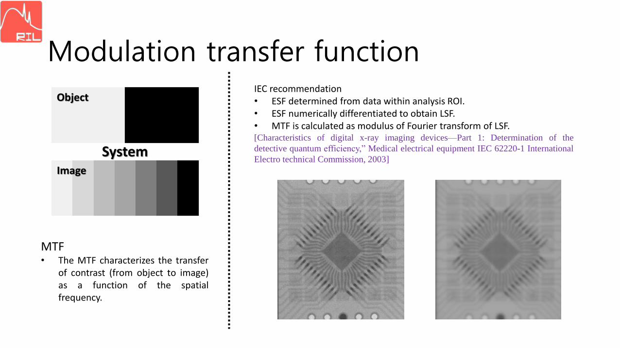
Modulation transfer function

MTF• The MTF characterizes the transfer

of contrast (from object to image)as a function of the spatialfrequency.

System

Object

Image

IEC recommendation• ESF determined from data within analysis ROI.• ESF numerically differentiated to obtain LSF.• MTF is calculated as modulus of Fourier transform of LSF.[Characteristics of digital x-ray imaging devices—Part 1: Determination of the

detective quantum efficiency,” Medical electrical equipment IEC 62220-1 International

Electro technical Commission, 2003]

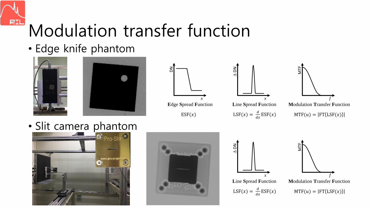
Modulation transfer function• Edge knife phantom

• Slit camera phantom

DN

x

DN

x f

MTF

Edge Spread Function Line Spread Function

LSF(𝑥) =𝑑

𝑑𝑥ESF(𝑥)

Modulation Transfer Function

MTF(𝑢) = FT LSF(𝑥)ESF(𝑥)

DN

x f

MTF

Line Spread Function

LSF(𝑥) =𝑑

𝑑𝑥ESF(𝑥)

Modulation Transfer Function

MTF(𝑢) = FT LSF(𝑥)

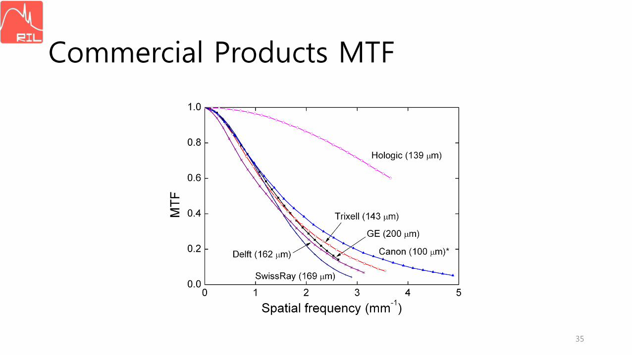
Commercial Products MTF

35