Discussion Papers In Economics And Business

Graduate School of Economics and Osaka School of International Public Policy (OSIPP)

Osaka University, Toyonaka, Osaka 560-0043, JAPAN

Relationship-specific Investment as a Barrier to Entry

Hiroshi Kitamura, Akira Miyaoka and Misato Sato

Discussion Paper 13-24

September 2013

Graduate School of Economics and Osaka School of International Public Policy (OSIPP)

Osaka University, Toyonaka, Osaka 560-0043, JAPAN

Relationship-specific Investment as a Barrier to Entry

Hiroshi Kitamura, Akira Miyaoka and Misato Sato

Discussion Paper 13-24

Relationship-specific Investment as a Barrier to Entry∗

Hiroshi Kitamura† Akira Miyaoka‡ Misato Sato§

September 16, 2013

Abstract

This study constructs a model of a relationship-specific investment in a dynamicframework. Although such investment decreases operating costs and increases the cur-rent joint profits of firms in vertical relationships, its specificity reduces the ex-post flex-ibility to change a trading partner in the future. We demonstrate that whether the invest-ment contract deters entry even in the absence of exclusionary terms depends on not onlythe specificity but also the efficiency of the investment. We also show that an increase inthe investment efficiency does not necessarily improve the equilibrium social welfare.

JEL Classifications Code: L12, L41, L42.Keywords: Vertical Relation; Entry Deterrence; Relationship-Specific Investment; Switch-ing Costs

∗We would like to thank Katsuya Takii, Reiko Aoki, Koki Arai, Hiroaki Ino, Akira Ishii, Hideshi Itoh,Masayuki Kanezaki, Keisuke Hattori, Noriaki Matsushima, Keizo Mizuno, Jun Nakabayashi, Hiroyuki Oda-giri, Jun Oshiro, Daniel Rubinfeld, Daisuke Shimizu, Tetsuya Shinkai, Mitsuru Sunada, Noriyuki Yanagawa,Takenobu Yuki, conference participants at the Japanese Association for Applied Economics, Japanese EconomicAssociation, and Institutions and Economics International Conference and seminar participants at HitotsubashiUniversity, Japan Fair Trade Commission, Kwansei Gakuin University, Osaka University, Osaka PrefectureUniversity, and Sapporo Gakuin University for helpful discussions and comments. We gratefully acknowledgefinancial support from JSPS Grant-in-Aid for Research Activity start-up No. 22830075, for Young Scientists(B) No. 24730220, for Scientific Research (A) No. 22243022, and for JSPS Fellows No. 12J01593 and finan-cial support from the Global COE program entitled “Human Behavior and Socioeconomic Dynamics” of OsakaUniversity. The usual disclaimer applies.

†Corresponding Author: Faculty of Economics, Kyoto Sangyo University, Motoyama, Kamigamo, Kita-Ku,Kyoto-City, Kyoto, 603-8555 Japan. E-mail: hiroshikitamura@cc.kyoto-su.ac.jp

‡Graduate School of Economics, Osaka University, 1-7 Machikaneyama, Toyonaka, Osaka, 560-0043,Japan. Email: jge013ma@mail2.econ.osaka-u.ac.jp

§Department of Economics, The George Washington University, 2115 G street, NW Monroe Hall 340 Wash-ington DC 20052, USA. Email: smisato@gwmail.gwu.edu

1 Introduction

In a number of vertical relationships, upstream firms make a relationship-specific investment

in downstream firms. For example, some firms develop original systems or instruments and

introduce them to downstream firms.1 Similarly, some firms provide special training pro-

grams to the downstream firm’s employees.2 These types of investments seem to decrease

the operating costs and increase the joint profits of firms in vertical relationships. In addition,

they seem to increase industry output and generate a socially efficient effect. From a static

viewpoint, these predictions are correct.

However, a relationship-specific investment usually generates specificity in vertical re-

lationships. For example, through special training programs or the introduction of original

systems, employees in downstream firms can establish specific routines (called “habitual rou-

tines”) for their operations with a current trading partner. Owing to such specificity, when

downstream firms change the trading partner, employees must usually unlearn these old rou-

tines before commencing operations with a new trading partner (Postrel and Rumelt, 1992).

This generates switching costs such as temporary performance degradation or an increase

in retraining costs for the ex-post change of the trading partner. Therefore, a relationship-

specific investment may deter efficient future entry and lead to socially inefficient outcomes

in a dynamic perspective.3

This study aims to theoretically explore the role of a relationship-specific investment as a

barrier to efficient entry and its welfare implication based on a dynamic framework. It con-

structs a two-period model of entry deterrence with the relationship-specific investment. In

the first period, one upstream incumbent exists but in the second period, a more efficient firm

appears. The upstream incumbent offers the single downstream firm an investment contract

with some fixed payments such as an introduction campaign for new systems or instruments

for a limited time.1For example, Ticketmaster, the leading ticket sales and distribution company in the United States, develops

an original system for concert venues. See Whinston (2006). See also Holden and O’Toole’s (2004) study, whichexplores the role of communication in determining the governance of manufacturer–retailer relationships.

2Ticketmaster also trains a venue’s personnel in the use of its system.3Postrel and Rumelt (1992) refer to the difficulty experienced by several companies such as Wedgwood and

Nucor in changing employees’ old habits. Further, in the psychological literature, Shiffrin and Schneider (1977)provide experimental evidence on this issue.

1

The key assumption in our model is that investment specificity generates switching costs

when the downstream firm changes its trading partner. When specificity is high, the accep-

tance of such investment restricts trading partner choices of the downstream firm because it

makes dealing with the entrant in the second period impossible. This exposes the downstream

firm to the intertemporal trade-off that once it accepts the specific investment, it becomes effi-

cient in the current period but cannot transact with an efficient entrant in the future. Therefore,

for examining the existence of entry deterrence, we need to focus on the downstream firm’s

incentive to accept or reject the investment.

In this setting, we explore the existence of entry deterrence because of the relationship-

specific investment and show that not only the investment specificity but also its efficiency

is an important factor that makes entry deterrence possible. To understand the importance of

investment efficiency in triggering entry deterrence, we begin by analyzing the case where the

investment is not efficient: that is, the investment does not reduce operating costs. We show

that the incumbent cannot then profitably design the investment contract to deter future entry

even when the investment is considerably specific. When the downstream firm rejects the

investment, the entrant offers a better wholesale price than the incumbent does in the second

period. This leads to a higher level of rejection profits for the downstream firm, which the

incumbent cannot profitably compensate under the investment contract.

In contrast, when the investment is efficient and reduces operating costs, the incumbent

can profitably design the investment contract to deter future entry if the investment is suffi-

ciently specific. In this case, the acceptance of investment increases the joint profits of the

incumbent and the downstream firm in the first period. We point out that this allows the

incumbent to profitably compensate the downstream firm’s rejection profits.

Our results imply that an improvement in investment efficiency can trigger entry deter-

rence. This leads to an important welfare implication that an improvement in investment ef-

ficiency does not necessarily increase the equilibrium social welfare; that is, the relationship

between the investment efficiency and equilibrium social welfare becomes non-monotonic.

Hence, our results suggest that we should have a dynamic perspective when we discuss the

welfare effect of relationship-specific investments. In a static view, such investment decreases

the current operating costs of firms in vertical relationships and improves social welfare.

2

However, in a dynamic view, the investment efficiency might reduce social welfare because

together with imposing switching costs, it can deter efficient future entry. Therefore, to eval-

uate the welfare effect of such investment, we need to consider these intertemporal effects.

Otherwise, we might obtain misleading predictions.

On interpreting our findings differently, our analysis predicts that entry deterrence owing

to an investment contract is more likely to be observed in an industry where downstream

firms are small companies. Small companies usually have fewer internal reserves and assets

because of difficulty in obtaining finance. Thus, upstream firms are more likely to need to

incur investment costs to develop instruments and systems for downstream firms.

This study is related to the literature on entry deterrence with switching costs.4 Klemperer

(1987) shows that entry deterrence is possible when the incumbent firm uses switching costs

in committing to a production capacity. In contrast, in the present study, entry deterrence

arises because switching costs restrict trading partner choices of the downstream firm and the

investment can increase the present joint profits of the firms in the vertical relationship.

This study is also related to the literature on entry deterrence through exclusive contracts.

In the 1970s, the Chicago School (Posner, 1976; Bork, 1978) argued that if we consider

downstream buyers’ incentives to accept exclusive contracts, rational economic agents would

not engage in exclusive dealing for anticompetitive reasons, and thus, entry deterrence is

impossible by using exclusive contracts. In rebuttal of the Chicago School argument, post-

Chicago economists show that entry deterrence is possible by using exclusive contracts in the

presence of scale economies5 (Rasmusen, Ramseyer, and Wiley, 1991; Segal and Whinston,

2000a) and downstream competition6 (Simpson and Wickelgren, 2007; Abito and Wright,

4Entry deterrence is analyzed in a number of studies wherein it arises owing to excess capacity (Spence,1977; Dixit, 1980), quality uncertainty (Schmalensee, 1982), and cost uncertainty (Milgrom and Roberts, 1982).

5Doganoglu and Wright (2010) explore exclusion in the presence of network externalities, which are anexample of scale economies. Fumagalli and Motta (2006) explore an extended model of Rasmusen, Ramseyer,and Wiley (1991) and of Segal and Whinston (2000a), where buyers are not final consumers but competingfirms. They show that intense downstream competition reduces the possibility of exclusion. However, Abitoand Wright (2008) point out that this result depends on the assumption that buyers are undifferentiated Bertrandcompetitors who need to incur epsilon participation fees to stay active and show that if buyers are differentiatedBertrand competitors, then intense downstream competition enhances exclusion. Wright (2009) also points outthat the equilibrium analysis of Fumagalli and Motta (2006) in the case of two-part tariffs contains some errorsand shows that exclusion arises when scale economies are sufficiently large or the entrant’s cost advantage isnot too big.

6See also Wright (2008), Argenton (2010), Kitamura (2010, 2011), Johnson (2012), Gratz and Reisinger

3

2008). The present study has a similar motivation because we explore entry deterrence by

considering downstream buyers’ incentive to accept an investment contract. In contrast to

earlier studies, however, this study shows that when a specific investment is made, the in-

vestment contract can deter efficient entry even in the absence of exclusionary terms, scale

economies, and downstream competition.

Exclusion with non-exclusive contracts has recently been analyzed by many economists

(Elhauge, 2009; Elhauge and Wickelgren, 2011, 2012a, and 2012b; Semenov and Wright,

forthcoming). These studies consider the design of wholesale pricing to deter efficient en-

trants and show that exclusion is possible even in the absence of exclusionary terms. The

present study shows another way of exclusion with non-exclusive contracts by using the in-

vestment contract.

Finally, this study is related to the literature on relationship-specific investments and ex-

clusive dealing (Marvel, 1982; Segal and Whinston, 2000b; De Meza and Selvaggi, 2007;

De Fontenay, Gans, and Groves, 2010). These studies examine the role of exclusive dealing

in enhancing the level of relationship-specific investment and show that exclusive dealing

may solve the hold-up problem and increase the level of investment in a specific market en-

vironment.7 In contrast, the present study focuses on the specificity of relationship-specific

investments as a barrier to future entry.

The reminder of this paper is organized as follows. Section 2 sets up the model. Section

3 analyzes the existence of entry deterrence because of the relationship-specific investment.

Section 4 explores the welfare implications of the investment. Section 5 discusses the ro-

bustness of our results under linear wholesale pricing. Finally, Section 6 contains concluding

remarks. Proofs of the results are provided in the Appendix.

(forthcoming), and Kitamura, Sato, and Arai (forthcoming).7Recently, in an extension to Segal and Whinston (2000b), Fumagalli, Motta, and Rønde (2012) show that

disregarding the interaction between investment promotion and market foreclosure may lead to misleading re-sults. They show that the investment promotion effect of exclusive dealing enhances anticompetitive exclusivedealing.

4

2 The model

This section sets up the model. We first characterize upstream and downstream markets in

2.1. Then, we introduce the timing of the game in 2.2.

2.1 Upstream and downstream markets

In the upstream market, two upstream firms exist, an incumbent (denoted byI ) and an entrant

(denoted byE). They produce an identical product but differ in cost efficiency. While the

incumbent has a marginal cost of productioncI , the entrant is more efficient and has a lower

marginal cost; that is,cE < cI .

In the downstream market, a monopolistic downstream firm exists (denoted byD).8 The

downstream firm purchases inputs from the upstream firm to produce a final product. We

assume that one unit of the final product requires one unit of the input and that the marginal

cost of transformation or resale iscD. We also assume that the demand for the final product

Q is given by a simple linear functionQ(p) = 1− p wherep is the final product’s price. We

also assume thatcI + cD < 1 such that selling to final consumers is at least profitable.

2.2 The timing of the game

The timing of the game follows that of Klemperer (1987) (see also Figure 1). The model

contains two periods (t = 1,2). At Period 1, only the incumbent exists in the upstream market.

This may be because of a patent right, efficient marketing, or an industry protection policy.

Period 1 consists of three stages. At Period 1.1, the incumbent offers the downstream firm

an investment contract involving some fixed compensationx ≥ 0. This offer is interpreted

as an introduction campaign for new systems or instruments developed by the incumbent

for a limited time.9 The investment reduces the marginal cost of the downstream firm for

the operation with the incumbent byd ∈ [0, cD). The level ofd is interpreted as the degree

8In the literature on anticompetitive exclusive dealing, in the absence of multiple downstream buyers, anupstream incumbent cannot deter efficient entry. Therefore, our modeling strategy of assuming a downstreammonopoly clarifies the role of investment as an entry barrier.

9As stated earlier, if downstream firms in an industry are small companies, they usually have limited internalreserves and assets because they cannot obtain finance easily. Thus, upstream firms are more likely to incurinvestment costs and offer a specific investment to downstream firms.

5

of investment efficiency. To simplify the analysis, we assume that the investment cost is

zero.10 The downstream firm decides to accept or reject this offer. We denote the decision

by θ ∈ {a, r}, whereθ = a (r) indicates the acceptance (rejection). We assume that when

the downstream firm is indifferent between accepting and rejecting the investment contract,

it accepts the contract.11

At Period 1.2, the incumbent offers wholesale contracts consisting of two-part tariffs

(wI |t=1, FI |t=1) ∈ R2+. In Section 5, we briefly discuss the case of linear wholesale pricing.12 At

Period 1.3, the downstream firm sells to final consumers. Note that because the incumbent

uses two-part tariffs, it optimally sets its per-unit wholesale price to equal its marginal cost

to remove the double marginalization problem; that is,wI |t=1 = cI . Therefore, if the down-

stream firm has accepted the investment contract at Period 1.1, then it operates atcI + cD − d.

However, if it has rejected the investment contract, then it operates atcI + cD (see also Table

1).

At Period 2, the entrant appears in the upstream market. Period 2 consists of four stages.

At Period 2.1, the entrant decides whether to enter the upstream market. We denote the

entrant’s decision byλ ∈ {in,out}, whereλ = in (out) indicates that the entrant enters (stays

out of) the market. We assume that the fixed cost of entry is negligible. Therefore, the

entrant always enters the market if its post-entry profits (gross of entry costs) are positive. At

Period 2.2, all active upstream firms offer wholesale contracts consisting of two-part tariffs

(wi|t=2, Fi|t=2), wherei ∈ {I ,E}, to the downstream firm. As in Period 1, active upstream firms

optimally set the per-unit wholesale prices to equal their marginal costs; that is,wi|t=2 = ci for

i ∈ {I ,E}.At Period 2.3, given the wholesale contracts offered by the upstream firm(s), the down-

stream firm decides on a trading partner. If the downstream firm deals with the incumbent

and has accepted the investment contract at Period 1, then the downstream firm operates at

10Introducing a positive investment cost does not alter our main results qualitatively.11If we assume that the downstream firm rejects the investment when it is indifferent, some of the arguments

in this study must be modified slightly. However, the essence of our results is still valid. See footnotes 18 and23 for details.

12Two-part tariffs allow us to illustrate our main results in a simpler way. As discussed in Section 5, althoughwe find almost the same results under linear wholesale pricing, the welfare analysis becomes considerablycomplicated.

6

cI + cD − d. If the downstream firm deals with the incumbent but has rejected the invest-

ment contract at Period 1, then the incumbent makes the investment offer again without fixed

compensationx and the downstream firm accepts the investment offer.13 As a result, the

downstream firm operates atcI +cD−d. On the other hand, if the downstream firm decides to

deal with the entrant, then the downstream firm operates atcE + cD.14 However, if the down-

stream firm has accepted the investment contract at Period 1, then it needs to incur switching

costsK > 0. The level of switching costs is interpreted as the degree of investment specificity.

For example, in the context of “habitual routines,” these switching costs include a temporary

performance degradation or an increase in the costs of familiarizing employees with a new

routine.15 We adopt the tie-break rule that when the downstream firm is indifferent between

dealing with the incumbent or the entrant, it continues to deal with the incumbent. At Period

2.4, the downstream firm orders the product produced by upstream firms and sells to final

consumers.

The incumbent’s and the downstream firm’s operating profits at Period 1 when the down-

stream firm’s investment decision at Period 1 isθ ∈ {a, r} are denoted byΠθI |t=1 andπθD|t=1,

respectively. Similarly, the incumbent’s, the downstream firm’s, and the entrant’s operating

profits at Period 2 when the downstream firm’s decision at Period 1 isθ ∈ {a, r} and the en-

trant’s decision at Period 2 isλ ∈ {in,out} are denoted byΠθ(λ)I |t=2, π

θ(λ)D|t=2, andΠ

θ(λ)E|t=2, respectively.

We assume no discounting between Period 1 and Period 2, for simplicity.16

Finally, in the analysis below, we assume that the following inequalities are satisfied:

13This is because the investment (at least) does not harm the downstream firm’s profits at Period 2.14We do not explicitly consider the investment between the entrant and the downstream firm. If the entrant

could offer the investment contract at Period 2, the downstream firm that decides to deal with the entrant alwaysaccepts the offer and this reduces the downstream firm’s operating costs to less thancE + cD. This does not alterour main results qualitatively.

15In this study, we assume that there is no switching cost when the downstream firm rejects the investmentcontract at Period 1. Of course, there can be a positive switching cost to change the trading partner even whenthe investment is not made. However, in the context of “habitual routines,” the ex-post change of trading partnercan be more costly when employees have established specific routines with the old partner than when they havenot. Therefore, our setting can be interpreted as one in which the general switching cost that does not dependon whether the investment is made is normalized to zero; we only focus on the switching cost owing to theinvestment specificity.

16Introducing a discount rateβ ∈ (0,1) between Period 1 and Period 2 does not change our results qualita-tively.

7

Assumption 1.

0 ≤ d < cI − cE ≤ cD. (1)

The second inequality guarantees that entry occurs at Period 2 as long as the investment

contract is rejected at Period 1. If the second inequality does not hold, the downstream firm

never deals with the entrant and entry never occurs at Period 2. The third inequality implies

that investment efficiencyd is in fact bounded bycI − cE and not bycD. This assumption

simplifies the analysis below.

3 Relationship-specific investment and entry deterrence

In this section, we analyze the existence of entry deterrence owing to the relationship-specific

investment. In 3.1, we describe the conditions to be satisfied so that the incumbent can deter

entry using an investment contract. In 3.2 and 3.3, we explore when these conditions are

actually satisfied. To understand easily the role of investment as an entry barrier, in 3.2, we

analyze the case where the investment is not efficient (d = 0) and in 3.3, we analyze the case

where the investment is efficient (d > 0).

3.1 Conditions for entry deterrence with a relationship-specific invest-ment

In this subsection, we describe the conditions to be satisfied for the incumbent to profitably

deter entry by using an investment contract. In brief, for the existence of entry deterrence

owing to a relationship-specific investment, the following two conditions must be satisfied

simultaneously:

Condition (i) Entry must be unprofitable for the entrant when the investment is undertaken

at Period 1.1,

Condition (ii) Entering into an investment contract at Period 1.1 must be profitable for both

the incumbent and the downstream firm.

In what follows, we describe these two conditions more formally.

8

3.1.1 Profitability of entry for the entrant

First, we examine Condition (i) and derive the condition that entry at Period 2.1 becomes

unprofitable for the entrant if the investment contract is made at Period 1.1. If the entrant

enters the market, the incumbent and the entrant compete for the downstream firm at Period

2.2. If the investment has been undertaken at Period 1.1, the downstream firm must incur

certain switching costs to change its trading partner. In this case, to attract the downstream

firm, the entrant must cover such switching costs in addition to guaranteeing the profits likely

to result for the downstream firm from the incumbent’s best offer. Therefore, we have the

following lemma that summarizes the condition under which entry at Period 2.1 becomes

unprofitable and the entrant does not enter the market:

Lemma 1. Suppose that the investment contract is made at Period 1.1. Then, the entrant

does not enter the market at Period 2.1 if and only if the investment is sufficiently specific or

efficient; that is, a pair of(K,d) satisfiesK ≥ K(d) andd ≥ 0 simultaneously, where

K(d) =(cI − cE − d)((1− (cI + cD − d)) + (1− (cE + cD)))

4, (2)

and whereK′(d) < 0 and limd→cI−cE K(d) = 0.

WhetherK ≥ K(d) holds depends on the degrees of investment specificityK, investment

efficiencyd, and entrant’s efficiencycE. Note that while the left-hand side ofK ≥ K(d) is

increasing inK, the right-hand side is decreasing in bothd andcE. As the investment becomes

more specific (asK increases), the downstream firm must incur larger switching costs to

change its trading partner at Period 2. Then, the entrant must offer a better wholesale contract

to induce the downstream firm to change its trading partner. Similarly, as the investment

becomes more efficient (asd increases), the entrant needs to offer a better wholesale contract

to the downstream firm. In these cases, it tends to be unprofitable for the entrant to enter the

market at Period 2.1. By contrast, as the entrant becomes more efficient (ascE decreases), it

can yield higher profits since the joint profits of the entrant and the downstream firm increase.

Therefore, market entry at Period 2.1 is more likely to be profitable for the entrant. Hence,

when the investment is highly specific but efficient and the entrant is not so efficient,K ≥ K(d)

is more likely to hold and the entrant tends to not enter the market at Period 2.1.

9

3.1.2 Investment contract design

Next, supposing thatK ≥ K(d) is satisfied, we examine Condition (ii) and derive the con-

dition that an investment contract deterring the efficient entrant needs to satisfy. Given the

equilibrium entry behavior of the entrant at Period 2.1, the equilibrium profits of the incum-

bent, entrant, and downstream firm in the subgames after Period 1.1 are summarized in Table

2.17 For the investment contract to be accepted at Period 1.1, it needs to satisfy the following

two conditions simultaneously.

First, the investment contract must satisfy financial feasibility for the incumbent: the

investment contract must enable the incumbent to yield higher profits, that is,

ΠaI |t=1 + Π

a(out)I |t=2 − x ≥ Πr

I |t=1 + ΠrI |t=2. (3)

Second, the investment contract must satisfy individual rationality for the downstream

firm: namely, the amount ofx must induce the downstream firm to accept the investment

contract, that is,

πaD|t=1 + πa(out)

D|t=2 + x ≥ πrD|t=1 + πr

D|t=2. (4)

From inequalities (3) and (4), we have the following inequality:

ΠaI |t=1 + Π

a(out)I |t=2 + πa

D|t=1 + πa(out)D|t=2 ≥ Πr

I |t=1 + ΠrI |t=2 + πr

D|t=1 + πrD|t=2. (5)

Inequality (5) implies that for the investment contract to be profitable for both the incumbent

and the downstream firm, this contract is required to at least increase the two-period joint

profits of contracting parties.

3.2 Benchmark: When investment is not efficient

From the discussion in 3.1, it is easy to see that the relationship-specific investment deters the

entrant if and only if inequalitiesK ≥ K(d) and (5) hold simultaneously. Now, we explore

when these conditions are actually satisfied. To understand easily the role of investment as

an entry barrier, in this subsection, we analyze the case where the investment is not efficient

(d = 0). In the next subsection, we analyze the case where the investment is efficient (d > 0).

17For the detailed derivation of the equilibrium offer and profit of each firm, see Appendix A.

10

Assume that the relationship-specific investment is not efficient; that is,d = 0. If in-

vestment specificityK is sufficiently low such thatK < K(0), then the downstream firm

can change the trading partner at Period 2 even when it accepts the investment at Period 1.

Then, the downstream firm tries to accept the investment at Period 1 and to deal with the en-

trant at Period 2. Therefore, the incumbent cannot deter the entrant by using the investment

contract.18

By contrast, if the investment is sufficiently specific such thatK ≥ K(0) holds, then the

acceptance of an investment contract induces the downstream firm to lose its best option of

accepting the investment contract at Period 1 but dealing with the entrant at Period 2. In such

a market environment, the downstream firm may strategically decide to reject the investment

offer so that it can deal with the entrant at Period 2. By considering the downstream firm’s

incentive to accept or reject the investment offer, the following proposition shows that when

the investment is not efficient, exclusion never occurs:

Proposition 1. Suppose that the relationship-specific investment is not efficient: d = 0. Then,

the incumbent cannot deter the efficient entrant even when the investment is sufficiently spe-

cific (even whenK ≥ K(0) holds).

The intuitive logic for the result underK ≥ K(0) is as follows (see also Figure 2). When

the downstream firm accepts the investment contract at Period 1, the entrant does not enter

the upstream market at Period 2 and only the incumbent offers wholesale contracts at both

Period 1 and Period 2. At each period, the joint profits of the incumbent and the downstream

firm coincide with monopoly profits for marginal costscI + cD.

However, when the downstream firm rejects the investment contract at Period 1, the en-

trant enters the upstream market, and the incumbent and the entrant compete for the down-

stream firm at Period 2. In the equilibrium, the downstream firm buys from the entrant under

a wholesale contract that leaves the downstream firm with slightly higher profits than the

monopoly profits for marginal costscI + cD. This implies that the acceptance of investment

18In this case, the incumbent accepts the investment owing to the assumption that if the downstream firm isindifferent between accepting and rejecting the investment contract, it accepts the contract. If instead we assumethat the downstream firm rejects the investment when it is indifferent, it is easy to see that the investment isrejected and the incumbent cannot deter the entrant.

11

reduces the two-period joint profits of the incumbent and the downstream firm; that is, in-

equality (5) does not hold. Therefore, the incumbent cannot profitably compensate the down-

stream firm for the rejection profits; that is, if the incumbent increasesx to satisfy inequality

(4), then inequality (3) does not hold.

3.3 When investment is efficient

We now assume that the relationship-specific investment is efficient; that is,d > 0. If invest-

ment specificityK is sufficiently low such thatK < K(d), the downstream firm can choose

its best option of accepting the investment contract at Period 1 but dealing with the entrant at

Period 2. Therefore, while the investment is always accepted, the incumbent cannot deter the

entrant with the investment contract.19

By contrast, if the investment is sufficiently specific such thatK ≥ K(d), the incumbent

can deter the efficient entrant unlike in the case whered = 0:

Proposition 2. The incumbent can deter the efficient entrant if and only if the investment is

not only specific but also efficient. More precisely, entry deterrence is possible for a pair of

(K,d) which satisfiesK ≥ K(d) andd > 0 simultaneously.

Figure 3 summarizes Proposition 2. To understand easily the results here, we provide the

intuitive logic by dividing the degree of investment specificity into two domains,K ≥ K(0)

andK < K(0). First, Figure 3 implies that when the investment specificity is sufficiently high

such thatK ≥ K(0), entry deterrence is possible in the presence of even small investment

efficiency d > 0. In this case, the crucial difference from the previous subsection arises

in the subgame after the downstream firm accepts the investment contract at Period 1 (see

also Figure 4). Unlike the case where the investment has no efficiency (d = 0), here, if the

downstream firm accepts the investment contract at Period 1, then the investment increases

the joint profits of the incumbent and the downstream firm at Period 1 to the monopoly profits

for marginal costscI + cD − d. An increase in the joint profits at Period 1 leads to an increase

19In this case, regardless of whether the investment contract is accepted at Period 1, the entrant always entersthe market at Period 2. This implies that while investing improves the joint profits of the incumbent and thedownstream firm at Period 1, it does not affect their joint profits at Period 2 (see Table 2). Therefore, thedownstream firm (strictly) prefers to accept the contract at Period 1 but to deal with the entrant at Period 2.

12

in the left-hand side of inequality (5) for alld > 0. This allows the incumbent to profitably

compensate the downstream firm for the rejection profits at Period 2.

Second, Figure 3 implies that when the investment specificity is sufficiently low such that

K < K(0), entry deterrence requires the higher investment efficiency d. In this case, the

investment is always accepted regardless of the level of investment efficiencyd. As discussed

in the interpretation of Lemma 1, an increase in investment efficiencyd forces the entrant to

offer better wholesale prices, which reduces the entrant’s post-entry profit. Therefore, for the

sufficiently efficient investment, entry is not profitable for the entrant when the investment

contract is accepted at Period 1. Since inequality (5) is satisfied for alld > 0, the incumbent

can deter the efficient entrant for the sufficiently higher investment efficiencyd that satisfies

K ≥ K(d).

Combining the results of Propositions 1 and 2, we obtain important insights into entry

deterrence under relationship-specific investment. The incumbent cannot exclude rivals only

with a specific investment: for exclusion, the investment needs to be not only specific but also

efficient.

Finally, note that our result in this section that entry deterrence can occur in the presence

of even small investment efficiencyd > 0 is due largely to the assumption of two-part tariff

contracts. In Section 5, we show that entry deterrence requires sufficiently higher efficiency

under linear wholesale pricing.

4 Relationship-specific investment and social welfare

In this section, we explore the welfare implications of the relationship-specific investment.

In 4.1, we analyze when the relationship-specific investment should be made from a social

welfare perspective by comparing the level of social welfare in the cases when the investment

is and is not made. In 4.2, we explore the relationship between the equilibrium social welfare

and investment efficiency.

13

4.1 Social desirability of the investment

In the previous section, we observed that in the equilibrium, the investment contract is always

accepted at Period 1 except when (K,d) satisfiesK ≥ K(0) andd = 0 simultaneously, as sum-

marized in Figure 3. In this subsection, by comparing the level of social welfare in the cases

when the investment is and is not made, we explore the conditions under which making the

relationship-specific investment is socially desirable (or undesirable).20 We analyze the two

types of investment separately, depending on whether the investment deters entry at Period 2.

In 4.1.1, we analyze the case where the investment deters entry. In 4.1.2, we analyze the case

where the investment does not deter entry.

4.1.1 When investment deters entry

We first assume that the investment is sufficiently specific that it deters the efficient entrant

at Period 2 (i.e.,K ≥ K(d) holds). In this case, the investment is accepted in the equilibrium

if and only if it is efficient. Therefore, here, we restrict our attention to the case ofd >

0. Let WINE denote the equilibrium level of social welfare (the superscriptINE stands for

“investment and no entry”), which is defined as follows:

WINE =3[1− (cI + cD − d)]2

8+

3[1− (cI + cD − d)]2

8. (6)

The first and second terms of the right-hand side of the above equation represent the

equilibrium level of social welfare at Period 1 and Period 2, respectively. In the equilibrium,

investing at Period 1 reduces the downstream firm’s marginal cost byd. However, such

investment also leads to entry deterrence and the downstream firm deals with the incumbent

at Period 2.

We compare this with the case where the investment is not made at Period 1. In the latter

case, although the downstream firm’s marginal cost is not reduced at Period 1, the efficient

entrant enters the upstream market and the downstream firm deals with the entrant at Period

20In this subsection, we explore the investment’s social desirability under the assumption that trading partnerchoices of the downstream firm at Period 2 are determined by the firms’ private incentives (i.e., whetherK ≥K(d) holds). Instead, if we assume that a social planner or the government could force the downstream firm todeal with the entrant at Period 2, the evaluation of the investment’s social desirability could be different fromthat in this subsection. Details are available from the authors upon request.

14

2. Let WNIE denote the levels of social welfare in this case (the superscriptNIE stands for

“no investment and entry”), which is defined as follows:

WNIE =3[1− (cI + cD)]2

8+

3[1− (cE + cD)]2

8. (7)

By comparing equations (6) and (7), we obtain the following proposition:

Proposition 3. Suppose that the relationship-specific investment is sufficiently specific such

that it leads to entry deterrence (K ≥ K(d)). Then, investing is socially desirable if and only

if this investment is sufficiently efficient; that is,WINE RWNIE if and only ifd R d, where

d =

√[1 − (cI + cD)]2 + [1 − (cE + cD)]2

2− (1− (cI + cD)) < cI − cE. (8)

The relationship-specific investment generates two contrary effects on social welfare.

First, the investment improves the efficiency of the vertical relationship between the incum-

bent and the downstream firm. Because this effect increases social welfare at Period 1, it can

be interpreted as the current benefit on investing. From equations (6) and (7), the current

benefitCB can be derived as the difference between the first terms of the right-hand sides of

equations (6) and (7), that is:

CB(d|K ≥ K(d)) =3[1− (cI + cD − d)]2

8− 3[1− (cI + cD)]2

8. (9)

Second, on the contrary, the investment deters the efficient entrant and this decreases

social welfare at Period 2. This effect can be regarded as the future loss on investing. The

future lossFL can be calculated as the difference between the second terms of the right-hand

sides of equations (6) and (7):

FL(d|K ≥ K(d)) =3[1− (cE + cD)]2

8− 3[1− (cI + cD − d)]2

8. (10)

By comparing equations (9) and (10), an increase in investment efficiencyd leads to dif-

ferent effects. On the one hand, the current benefit is increasing ind because the efficient

investment increases the social welfare at Period 1. On the other hand, the future loss is

decreasing ind because welfare loss at Period 2 decreases for the efficient investment. There-

fore, if the investment is sufficiently efficient (d > d), then the current benefit dominates the

future loss and the investment becomes socially desirable.

15

4.1.2 When investment does not deter entry

We next assume that the investment is not so specific and that it allows entry by an efficient

entrant at Period 2 (that is,K < K(d) holds). In the equilibrium for this market environment,

the investment contract withd ≥ 0 is always accepted at Period 1 but the efficient entrant

enters the upstream market and the downstream firm deals with the entrant at Period 2. Let

WIE denote the equilibrium levels of social welfare in this case (the superscriptIE stands for

“investment and entry”), which is defined as follows:

WIE =3[1− (cI + cD − d)]2

8+

[3[1− (cE + cD)]2

8− K

]. (11)

One of the important features ofWIE is represented in the brackets of the right-hand side

of equation (11). Although the entry occurs at Period 2, the downstream firm needs to incur

switching costK, which constitutes the social cost, to deal with the entrant.21 This implies

that the investment may be socially undesirable even when it does not lead to entry deterrence

at Period 2.

As in 4.1.1, we compare this with the case where the investment is not made at Period 1.

In the latter case, although the downstream firm’s marginal cost is not reduced at Period 1, the

entrant enters the upstream market and the downstream firm deals with the entrant without

switching costs at Period 2. Therefore, the level of social welfare in this case coincides with

WNIE, represented by equation (7). By comparing equations (7) and (11), we obtain the fol-

lowing proposition, which shows when the investment that does not lead to entry deterrence

becomes socially desirable:

Proposition 4. Suppose that the relationship-specific investment is not so specific and that it

allows entry at Period 2 (K < K(d)). Then, investing is socially desirable if and only if this

investment is not so specific or is sufficiently efficient. More precisely,

1. When the investment is sufficiently efficient (ford > d) or within an intermediate range

of efficiency (ford < d ≤ d), investing is always socially desirable; that is,WIE > WNIE

21In this model, switching costK could be interpreted as damages for breach of contract. However, in thatcase,K is just a monetary transfer between firms and does not affect the social welfare. Alternatively, in thisstudy, we considerK as, for example, a temporary performance degradation, which harms social welfare.

16

always holds, where

d =

√3[1− (cI + cD)]2 + 2[1− (cE + cD)]2

5− (1− (cI + cD)), (12)

and

2. When the investment is not too efficient (for d ≤ d), investing is socially desirable if

and only if the investment specificity is sufficiently low; that is,WNIE RWIE if and only

if K R K(d), where:

K(d) =3d((1− (cI + cD − d)) + (1− (cI + cD)))

8. (13)

As in the case of the investment that leads to entry deterrence in 4.1.1, the investment that

does not deter entry also has two contrary effects on social welfare: a current benefit and a

future loss. First, the investment improves the vertical relationship’s efficiency and increases

social welfare at Period 1. From the first terms of the right-hand sides of equations (7) and

(11), this current benefit on investing is the same as that in 4.1.1:

CB(d|K < K(d)) =3[1− (cI + cD − d)]2

8− 3[1− (cI + cD)]2

8. (14)

Second, on the contrary, the investment generates a future loss that is different from the

future loss in 4.1.1. In contrast to 4.1.1, here, investing does not lead to entry deterrence.

However, it requires the downstream firm to incur switching costK to deal with the entrant

at Period 2. This becomes the future loss to make the investment that does not deter entry:

FL(d|K < K(d)) = K. (15)

The comparison between equations (14) and (15) implies that the current benefit is in-

creasing in investment efficiencyd but the future loss is not. It also implies that the current

benefit does not depend on investment specificityK but that the future loss is increasing in

K. Therefore, if the investment efficiency is sufficiently high or the switching cost is not too

high, then the current benefit is predominant and such investing improves social welfare.

The results of Propositions 3 and 4 are summarized in Figure 5. Note that the curve

K = K(d), which we derived in Lemma 1, represents the critical values ofK above which

17

Proposition 3 applies and below which Proposition 4 applies. From Figure 5, it can be seen

that overall, a relationship-specific investment is socially desirable when its efficiency is suf-

ficiently high. This implies that a high-efficiency investment is more likely to improve social

welfare than a low-efficiency one. However, as we explain below, a close look at Figure 5

reveals that this argument does not always hold.

Figure 5 shows that for an intermediate level of investment specificity (i.e., forK ∈(K(d), K(d))), there is a non-monotonic relationship between the investment’s social desir-

ability and its degree of efficiency. More precisely, as the investment becomes more efficient,

the welfare property of the investment shifts from socially undesirable to desirable, then back

to undesirable, and, finally, to desirable.

This result reflects the property of the future loss on investing; the future loss discontin-

uously changes according to investment efficiencyd. In contrast to the current benefit, the

future loss differs in the cases when the investment deters and does not deter entry. In the for-

mer case, the future loss is derived from the failure of efficient entry owing to the existence

of a switching cost (equation (10)). By contrast, when the investment does not deter entry,

the future loss is derived from the switching cost itself (equation (15)).

Figure 6 illustrates the property of future loss for an intermediate level of specificity.

Figure 6 shows that if investment efficiencyd increases above the threshold valued2, then

the future loss increases discontinuously. At this increase ofd, the equilibrium outcome at

Period 2 moves from entry to entry deterrence. Because entry deterrence leads to higher

market prices and to a smaller level of consumer surplus, the change of equilibrium outcome

reduces the social welfare at Period 2. This leads to a discontinuous change in future loss.

By comparing the future loss and the current benefit in Figure 6, an increase in the invest-

ment efficiency (ford ∈ [d1,d2)) first makes the investment socially desirable as the current

benefit increases and dominates the future loss. However, a further increase in efficiency (for

d ∈ [d2,d)) enables the investment to deter entry at Period 2 and this raises the future loss

discontinuously, thereby making the investment socially undesirable. Finally, as the invest-

ment becomes sufficiently efficient (ford ≥ d), the current benefit on investing dominates the

future loss again. Therefore, investing becomes socially desirable.

18

4.2 Social welfare and investment efficiency

In this subsection, for a given degree of specificityK, we explore how a change in invest-

ment efficiencyd ≥ 0 affects the equilibrium social welfare. Intuitively, an improvement in

investment efficiency decreases the operating costs and thus increases the equilibrium social

welfare. This view seems correct because it is easy to see thatWINE andWIE are increasing

in d from equations (6) and (11).22

However, the following proposition shows that the possibility of entry deterrence trig-

gered by the investment efficiency leads to a non-monotonic relationship between the invest-

ment efficiency and equilibrium social welfare:

Proposition 5. For a given degree of specificityK, the equilibrium social welfare is increas-

ing in investment efficiencyd except where it discontinuously decreases by triggering entry

deterrence. More precisely, a slight improvement in investment efficiencyd aroundd(K) re-

duces the equilibrium social welfare, where

d(K) =

0 f or K ≥ K(0),√

(1− (cE + cD))2 − 4K − (1− (cI + cD)) f or K < K(0).(16)

Note thatd(K) for K < K(0) is the inverse function ofK(d) (see equation (2)). When

K ≥ K(0), the investment contract is rejected and entry occurs underd = 0. However, the

presence of (even small) investment efficiency enables the contract to be accepted and entry

deterrence occurs. Therefore, as the investment efficiency increases from zero to positive, the

equilibrium social welfare changes fromWNIE to WINE.

By contrast, whenK < K(0), the investment contract is accepted for anyd ≥ 0. However,

whether entry deterrence occurs still depends on the investment efficiency. In this case, by

making entry less profitable for the entrant, the higher investment efficiency leads to entry

deterrence. Therefore, as the investment efficiency increases aboved(K), the equilibrium

social welfare changes fromWIE to WINE.23 These discontinuous changes for bothK ≥ K(0)

22From equation (7), it is easy to see thatWNIE is independent of investment efficiencyd.23If we assume that the downstream firm rejects an investment contract when it is indifferent, the investment

is accepted only ford > 0 also underK < K(0). Therefore, the equilibrium social welfare underK < K(0)discontinuously changes not only aroundd = d(K) but also aroundd = 0. In the latter case, as the investmentefficiency slightly increases from zero to positive, the equilibrium social welfare underK < K(0) changes fromWNIE to WIE . Proposition 4 implies that this discontinuous change reduces the equilibrium social welfare.

19

andK < K(0) reduce the equilibrium social welfare.

The results in this section clarify the importance of a dynamic perspective for the discus-

sion of relationship-specific investments. In a static view, the investment efficiency decreases

operating costs among vertical relations and has a welfare improving effect. However, in

a dynamic view, the investment specificity generates a switching cost to change the trading

partner and has a welfare reducing effect regardless of whether the investment deters future

entry. In addition, from a dynamic perspective, an improvement in investment efficiency does

not necessarily increase social welfare, because it can trigger entry deterrence. Therefore, to

consider the welfare effect of the investment, we need to consider these intertemporal effects

of the investment. Otherwise, we may obtain misleading predictions.

5 Linear wholesale pricing

In this section, we briefly discuss the case when the upstream firms can use only linear whole-

sale pricing. For analysis, we make an additional assumption as follows:

Assumption 2.

cI − d <1− cD + cE

2. (17)

Note that the right-hand side of this inequality represents a monopoly wholesale price by

the entrant. It is easy to see that this inequality is more likely to hold whencI is small orcE is

large. This assumption implies that the entrant’s cost advantage is so small that it cannot set

the monopoly price in wholesale competition with the incumbent.24 Combining Assumptions

1 and 2, under linear wholesale pricing, we restrict our attention to investment efficiencyd,

which satisfies the following inequality:

max

{(cI − cE) − (1− (cD + cI ))

2,0

}< d < cI − cE. (18)

In the case of linear wholesale pricing, as the next proposition shows, we have qualitatively

the same results as under two-part tariffs but the investment efficiency becomes more impor-

tant to trigger entry deterrence.

24A similar assumption is often made in the exclusive dealing literature (e.g., Fumagalli and Motta, 2006;Abito and Wright, 2008; Kitamura, 2010). Entry deterrence can still occur without this assumption, but theanalysis becomes more complicated.

20

Proposition 6. Suppose that the upstream firms can only use linear wholesale contracts.

Then, the incumbent can deter the efficient entrant through the investment contract if and

only if the investment is sufficiently specific and efficient; that is, a pair of(K,d) satisfies

K ≥ K(d) andd > d simultaneously, where

d =

√6− 22

(1− (cD + cI )) > 0, (19)

and where(√

6− 2)/2 ≈ 0.2247.

Recall that under two-part tariffs, entry deterrence under the investment contract occurs

if and only if K ≥ K(d) and d > 0 (Proposition 2). Unlike under two-part tariffs, entry

deterrence under linear wholesale pricing requires asufficiently higher efficiency; that is,

d > d > 0.25 Figure 7 illustrates the result of Proposition 6 whend falls within the range of

inequality (18).26

In the case of linear wholesale pricing, the major difference from the case of two-part

tariffs is the presence of a double marginalization problem. UnderK ≥ K(d), when the in-

vestment contract is accepted, the incumbent maintains a monopoly throughout both periods

and the double marginalization problem reduces the joint profits of the incumbent and the

downstream firm in both periods. By contrast, when the investment contract is rejected, that

problem reduces the joint profits of the incumbent and the downstream firm only at Period

1 because the wholesale price competition between the incumbent and the entrant eliminates

the problem at Period 2. This means that the left-hand side of inequality (5) decreases more

significantly than the right-hand side. Therefore, under linear wholesale pricing, condition

(5) becomes tighter and the investment needs to be still more efficient than the one under

two-part tariffs.

In relation to the welfare implications of the investment under linear wholesale pricing,

various cases arise depending on the parameter values and the analysis becomes considerably

25d falls within the range of inequality (18) if and only if√

6/2 < (1− (cD + cE))/(1− (cD + cI )) <√

6. When(1− (cD + cE))/(1− (cD + cI )) ≤

√6/2, we haved ≥ cI − cE and the incumbent can never deter the entrant with

the investment contract that satisfies inequality (18). By contrast, when (1− (cD + cE))/(1− (cD + cI )) ≥√

6, wehaved ≤ [(cI − cE) − (1− (cD + cI ))]/2 and the incumbent can always deter the entrant under inequality (18).

26As Figure 7 shows, underK < K(d), the investment contract is accepted but entry occurs regardless of thevalue ofd. This is for the same reason as under two-part tariffs. See footnote 19.

21

complicated. However, whend falls within the range of inequality (18), we obtain results

similar to those under two-part tariffs: first, investing tends to be socially desirable when

the investment is not so specific but highly efficient; second, the equilibrium social welfare

discontinuously decreases asd exceeds the threshold valued.

6 Concluding remarks

This study explored the role of relationship-specific investment as a barrier to efficient entry.

The investment generates switching costs to change the trading partner, thereby reducing the

downstream firm’s ex-post flexibility to deal with the efficient entrant in the future. However,

the investment also increases the current joint profits of the incumbent and the downstream

firm. We showed that because ofboth the switching costs and an increase in current joint

profits, the incumbent could deter the efficient entrant in the future by using an investment

contract. We also showed that the investment’s welfare effect depends on both its specificity

and efficiency and that an increase in the investment efficiency can reduce the equilibrium

social welfare.

These results provide an important policy implication. When we discuss the welfare effect

of a relationship-specific investment, we need to have a dynamic perspective. From a static

perspective, the investment reduces current operating costs among vertical relationships and

it seems to be efficient. From a dynamic perspective, however, the investment efficiency

itself enables the investment contract to be accepted even when it generates switching costs

to change a trading partner in the future. Therefore, the seemingly efficient investment can

also be the cause of inefficiency. To evaluate the relationship-specific investment correctly,

we need to pay attention to both of these opposing effects on social welfare.

By interpreting our results differently, we obtain an important policy implication that an

inefficient firm may survive for a long time because of relationship-specific investments. In

the international trade literature, a number of economists argue that vertical relationships

within Japanese companies, known askeiretsu, play the role of a structural trade barrier (e.g.,

Lawrence, 1991, 1993a, and 1993b; Spencer and Qiu, 2001).27 One important feature of

27In the Structural Impediments Initiative (SII) between Japan and the United States during 1989–1990,particular attention was paid to the role ofkeiretsu. The U.S. government argued thatkeiretsulinkages made

22

keiretsuis that relationship-specific investments are common among its members, for exam-

ple, as in the auto industry. Our results might be one possible explanation of why foreign

firms cannot easily enter the Japanese market in the presence of relationship-specific invest-

ments withinkeiretsugroups.

Several outstanding issues require future research. First, there is a concern about the gen-

erality of our results. Although our analysis is in terms of a parametric example, the results

may extend to more general settings. Second, a concern about the role of strategic interac-

tion between downstream firms exists. In our model, a downstream firm is a monopolist in

its final product market. However, the competition between downstream firms is an impor-

tant research topic. We predict that, as discussed by Simpson and Wickelgren (2007) and

Abito and Wright (2008) in their studies on anticompetitive exclusive dealing, competition

between downstream firms enables the upstream incumbent to deter efficient entry under the

relationship-specific investment more easily.

Finally, a concern about the incumbent’s strategic behavior exists. According to our re-

sults, the incumbent may have an incentive to control the investment specificity. For example,

its investment may be too specific. We trust that this study will assist future researchers in

addressing these issues.

A Equilibria in the subgame following Period 1.1

In this Appendix, we analyze the equilibrium in each of the possible subgames after Period

1.1. Especially, we explore the wholesale contracts offered by upstream firms, realized profit

of each firm, and entry behavior of the entrant in the equilibrium of each subgame.

foreign entry into the Japanese market difficult. At the end of the SII talks, the Japanese government agreedto strengthen monitoring by its Fair Trade Commission of transactions amongkeiretsufirms and to take thenecessary steps toward eliminating any restraints on competition that might arise from their business practices(Lawrence, 1993b).

23

A.1 When the downstream firm accepts the investment contract at Pe-riod 1.1

First, suppose that the downstream firm accepts the relationship-specific investment at Period

1.1. At Period 1.2, to solve the double marginalization problem, the incumbent sets its per-

unit wholesale price to equal its marginal cost and extracts all of the downstream firm’s profit

through the fixed fee; that is, the incumbent offers the following wholesale contract:

(wI |t=1, FI |t=1) =

(cI ,

[1 − (cI + cD − d)]2

4

). (20)

Therefore, the incumbent and the downstream firm respectively yield the following operating

profits at Period 1.3:

ΠaI |t=1 =

[1 − (cI + cD − d)]2

4,

πaD|t=1 = 0.

(21)

At Period 2.1, the entrant decides whether to enter the upstream market. If the entrant

does not enter the upstream market, the incumbent monopolizes the market and offers the

same wholesale contract as at Period 1. Therefore, the equilibrium operating profits for the

incumbent, the entrant, and the downstream firm respectively become

Πa(out)I |t=2 =

[1 − (cI + cD − d)]2

4,

Πa(out)E|t=2 = 0,

πa(out)D|t=2 = 0.

(22)

By contrast, when the entrant enters the upstream market, the incumbent and the entrant com-

pete for the downstream firm at Period 2.2. While the incumbent’s best offer (wI |t=2, FI |t=2) =

(cI ,0) leaves the downstream firm with [1−(cI+cD−d)]2/4, the entrant’s best offer (wE|t=2, FE|t=2) =

(cE,0) leaves the downstream firm with [1− (cE + cD)]2/4− K.28 Therefore, which upstream

firm profitably captures the downstream firm depends on the specificity and efficiency of the

investment. First, if [1− (cI + cD − d)]2/4 ≥ [1 − (cE + cD)]2/4− K, which is equivalent to

28Note that since the downstream firm has accepted the investment contract at Period 1.1, it must incurswitching costs to change the trading partner to the entrant at Period 2.

24

K ≥ K(d), the downstream firm’s switching costs are so high that the incumbent can prof-

itably attract the downstream firm.29 Anticipating that the post-entry profit is zero, the entrant

does not enter the market in the equilibrium (owing to negligible entry costs). Therefore, in

this case, the equilibrium profit of each firm at Period 2 is given by equation (22).

Second, if [1− (cI +cD−d)]2/4 < [1− (cE +cD)]2/4−K, which is equivalent toK < K(d),

the level of switching costs is low enough for the entrant to profitably attract the downstream

firm. In this case, the incumbent and the entrant offer the following wholesale contracts:

(wI |t=2, FI |t=2) = (cI ,0),

(wE|t=2, FE|t=2) =

(cE,

[1 − (cE + cD)]2

4−

[[1 − (cI + cD − d)]2

4+ K + ε

]),

(23)

whereε is some infinitesimally small number.30 At Period 2.3, the downstream firm chooses

the entrant as the trading partner. At Period 2.4, each firm yields the following operating

profits:

Πa(in)I |t=2 = 0,

Πa(in)E|t=2 =

[1 − (cE + cD)]2

4−

[[1 − (cI + cD − d)]2

4+ K + ε

],

πa(in)D|t=2 =

[1 − (cI + cD − d)]2

4+ ε.

(24)

Therefore, anticipating that the post-entry profit is strictly positive, the entrant enters the

market at Period 2.1 in the equilibrium.

A.2 When the downstream firm rejects the investment contract at Pe-riod 1.1

Next, suppose that the downstream firm rejects the relationship-specific investment at Period

1.1. At Period 1.2, the incumbent offers the following wholesale contract:

(wI |t=1, FI |t=1) =

(cI ,

[1 − (cI + cD)]2

4

). (25)

29The incumbent can do this by offeringwI |t=2 = cI and choosing the fixed fee that makes the downstreamfirm indifferent between its offer and the entrant’s:FI |t=2 = [1 − (cI + cD − d)]2/4−

[[1 − (cE + cD)]2/4− K

].

30The entrant sets the per-unit wholesale price at the marginal cost level and chooses the fixed fee that leavesthe downstream firm with slightly more profit than the incumbent’s best offer.

25

Therefore, at Period 1.3, the incumbent and the downstream firm respectively yield:

ΠrI |t=1 =

[1 − (cI + cD)]2

4,

πrD|t=1 = 0.

(26)

At Period 2.1, the entrant decides whether to enter the market. If the entrant enters the

upstream market, the incumbent and the entrant compete for the downstream firm at Period

2.2. While the incumbent’s best offer leaves the downstream firm with [1− (cI + cD − d)]2/4,

the entrant’s best offer leaves the downstream firm with [1− (cE + cD)]2/4.31 Therefore, the

entrant can profitably capture the downstream firm. In the equilibrium, the incumbent and

the entrant respectively offer the following wholesale contracts:

(wI |t=2, FI |t=2) = (cI ,0) ,

(wE|t=2, FE|t=2) =

(cE,

[1 − (cE + cD)]2

4−

[[1 − (cI + cD − d)]2

4+ ε

]).

(27)

Then, the downstream firm decides to deal with the entrant and each firm yields the following

operating profits:

ΠrI |t=2 = 0,

ΠrE|t=2 =

[1 − (cE + cD)]2

4−

[[1 − (cI + cD − d)]2

4+ ε

],

πrD|t=2 =

[1 − (cI + cD − d)]2

4+ ε.

(28)

Therefore, anticipating the positive post-entry profit, the entrant enters the market at Period

2.1 in the equilibrium.

B Proofs

Proof of Lemma 1

Note that since we assume negligibly small entry costs, the entrant does not enter the market

if and only if its post-entry profit is less than or equal to zero. If the entrant enters the market,

the incumbent and the entrant compete for the downstream firm at Period 2.2. While the

31Since the downstream firm has rejected the investment contract at Period 1.1, there are no switching costsfor the downstream firm to change its trading partner.

26

incumbent’s best offer leaves the downstream firm with [1− (cI + cD − d)]2/4, the entrant’s

best offer leaves the downstream firm with [1− (cE + cD)]2/4− K. Therefore, if

[1 − (cI + cD − d)]2

4≥ [1 − (cE + cD)]2

4− K (29)

holds, the incumbent profitably attracts the downstream firm and the entrant’s post-entry

profit becomes zero. By solving this inequality with respect toK, we haveK ≥ K(d).

Q.E.D.

Proof of Proposition 1

See the proof of Proposition 2.

Q.E.D.

Proof of Proposition 2

Recall that the relationship-specific investment deters the entrant if and only if both of in-

equalitiesK ≥ K(d) and (5) hold. Substituting equilibrium profits (see Table 2 or Appendix

A) into inequality (5), it can be rewritten as follows:

2

([1 − (cI + cD − d)]2

4

)≥ [1 − (cI + cD)]2

4+

[1 − (cI + cD − d)]2

4+ ε. (30)

It is easy to see that this inequality holds if and only ifd > 0. Therefore, whend = 0,

inequality (30) does not hold and incumbent cannot profitably induce the downstream firm

to accept the investment contract, even ifK ≥ K(d) underd = 0 is satisfied (Proposition 1).

On the other hand, whend > 0, inequality (30) always holds and the incumbent can deter the

efficient entrant if and only ifK ≥ K(d) is satisfied (Proposition 2).

Q.E.D.

Proof of Proposition 3

From equations (6) and (7), we have

WINE RWNIE ⇔ 3[1− (cI + cD − d)]2

4R

3[1− (cI + cD)]2

8+

3[1− (cE + cD)]2

8

⇔ d R

√[1 − (cI + cD)]2 + [1 − (cE + cD)]2

2− (1− (cI + cD)).

(31)

27

Let d denote the right-hand side of last inequality. Then, we haveWINE R WNIE if and only

if d R d.

Q.E.D.

Proof of Proposition 4

From equations (7) and (11), we have

WNIE RWIE ⇔ 3[1− (cI + cD)]2

8R

3[1− (cI + cD − d)]2

8− K

⇔ K R3d((1− (cI + cD − d)) + (1− (cI + cD)))

8.

(32)

Let K(d) denote the right-hand side of last inequality. It is easy to see that∂K(d)/∂d > 0

and K(0) = 0. Recall that we now consider the case ofK < K(d). From the properties of

K(d) andK(d), there existsd ∈ (0, cI − cE) such thatK(d) = K(d). Then,d can be obtained

as equation (12) and it is easy to see thatd < d. Whend > d, we haveK < K(d) < K(d).

Therefore,WNIE < WIE always holds. On the other hand, whend ≤ d, we haveK(d) ≥ K(d).

Therefore, we haveWNIE RWIE if and only if K R K(d).

Q.E.D.

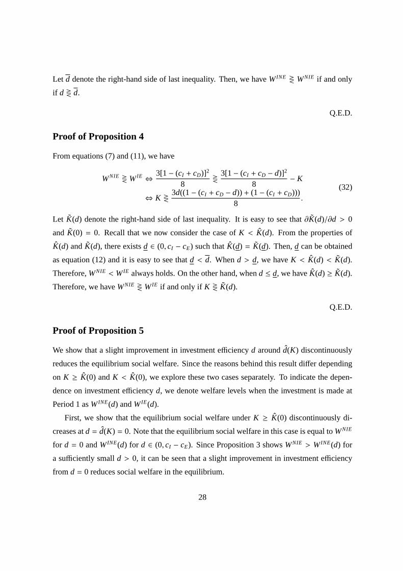
Proof of Proposition 5

We show that a slight improvement in investment efficiencyd aroundd(K) discontinuously

reduces the equilibrium social welfare. Since the reasons behind this result differ depending

on K ≥ K(0) andK < K(0), we explore these two cases separately. To indicate the depen-

dence on investment efficiencyd, we denote welfare levels when the investment is made at

Period 1 asWINE(d) andWIE(d).

First, we show that the equilibrium social welfare underK ≥ K(0) discontinuously di-

creases atd = d(K) = 0. Note that the equilibrium social welfare in this case is equal toWNIE

for d = 0 andWINE(d) for d ∈ (0, cI − cE). Since Proposition 3 showsWNIE > WINE(d) for

a sufficiently smalld > 0, it can be seen that a slight improvement in investment efficiency

from d = 0 reduces social welfare in the equilibrium.

28

Next, we show that the equilibrium social welfare underK < K(0) discontinuously di-

creases atd = d(K) =√

(1− (cE + cD))2 − 4K−(1−(cI +cD)). Note that the equilibrium social

welfare in this case is equal toWIE(d) for d ∈ [0, d(K)) andWINE(d) for d ∈ [d(K), cI − cE).

From equations (6) and (11), we have

limd→d(K)−0

WIE(d) =3(1− (cE + cD))2

4− 5

2K,

WINE(d(K)) =3(1− (cE + cD))2

4− 3K,

(33)

and it is easy to see that limd→d(K)−0 WIE(d) > WINE(d(K)). Therefore, the equilibrium social

welfare discontinuously decreases whend exceeds or even equalsd(K).

Q.E.D.

Proof of Proposition 6

As in the case of two-part tariffs, for the existence of entry deterrence under linear wholesale

pricing, the two conditions mentioned in Subsection 3.1 must be satisfied simultaneously.

First, entry at Period 2.1 must be unprofitable for the entrant if the investment contract

is accepted at Period 1.1. Note that the entrant does not enter the market if and only if its

post-entry profit is less than or equal to zero. If the entrant enters the market, the incumbent

and the entrant compete for the downstream firm at Period 2.2. While the incumbent’s best

offerwI |t=2 = cI leaves the downstream firm with [1− (cI + cD−d)]2/4, the entrant’s best offer

wE|t=2 = cE leaves the downstream firm with [1− (cE + cD)]2/4− K. Therefore, if

[1 − (cI + cD − d)]2

4≥ [1 − (cE + cD)]2

4− K (34)

holds, the incumbent profitably attracts the downstream firm and the entrant’s post-entry

profit becomes zero. By solving this inequality with respect toK, we haveK ≥ K(d).

Next, supposing thatK ≥ K(d) is satisfied, an investment contract which deters the ef-

ficient entrant must be profitable for both the incumbent and the downstream firm, that is,

inequality (5) must be satisfied. Below, we derive the equilibrium profit of each firm in the

possible subgames after Period 1.1.

29

First, suppose that the downstream firm accepts the investment contract at Period 1.1. At

Period 1.2, as an upstream monopolist, the incumbent offerswI |t=1 = (1 − (cD − d) + cI )/2.

Therefore, the incumbent and the downstream firm respectively yield the following operating

profits at Period 1.3:

ΠaI |t=1 =

[1 − (cI + cD − d)]2

8,

πaD|t=1 =

[1 − (cI + cD − d)]2

16.

(35)

At Period 2.1, assumingK ≥ K(d) holds, the entrant does not enter the upstream market.

In this case, the incumbent offers the same wholesale price as at Period 1, and the equilibrium

operating profits for the incumbent, the entrant, and the downstream firm respectively become

Πa(out)I |t=2 =

[1 − (cI + cD − d)]2

8,

Πa(out)E|t=2 = 0,

πa(out)D|t=2 =

[1 − (cI + cD − d)]2

16.

(36)

Suppose next that the downstream firm rejects the investment contract at Period 1.1. At

Period 1.2, the incumbent offers wI |t=1 = (1 − cD + cI )/2. Therefore, at Period 1.3, the

incumbent and the downstream firm respectively yield:

ΠrI |t=1 =

[1 − (cI + cD)]2

8,

πrD|t=1 =

[1 − (cI + cD)]2

16.

(37)

At Period 2.1, the entrant makes the entry decision. When it enters the upstream market,

the incumbent and the entrant compete for the downstream firm at Period 2.2. While the

incumbent’s best offerwI |t=2 = cI leaves the downstream firm with [1− (cI + cD − d)]2/4, the

entrant’s best offer wE|t=2 = cE leaves the downstream firm with [1− (cE + cD)]2/4. From

Assumption 1, it is easy to see that the entrant can profitably capture the downstream firm.

Therefore, in equilibrium, the entrant always enters the market and the entrant’s wholesale

price becomeswE|t=2 = cI − d − ε, whereε is some infinitesimally small number, from

30

Assumption 2. Then, each firm yields the following operating profits:

ΠrI |t=2 = 0,

ΠrE|t=2 =

(cI − cE − d)(1− (cI + cD − d))2

,

πrD|t=2 =

[1 − (cI + cD − d)]2

4+ ε.

(38)

By substituting above equilibrium profits in each case into inequality (5), it can be rewrit-

ten as follows:

2

(3[1− (cI + cD − d)]2

16

)≥ 3[1− (cI + cD)]2

16+

[1 − (cI + cD − d)]2

4+ ε. (39)

By rearranging this inequality, we have inequality (19). Therefore, under linear wholesale

pricing, the incumbent can deter the efficient entrant if and only if inequalitiesK ≥ K(d) and

(19) are both satisfied.

Q.E.D.

References

Abito, J.M., and Wright, J., 2008.Exclusive Dealing with Imperfect Downstream Competi-

tion. International Journal of Industrial Organization26(1), 227–246.

Argenton, C., 2010.Exclusive Quality.Journal of Industrial Economics58(3), 690–716.

Bork, R.H., 1978.The Antitrust Paradox: A Policy at War with Itself.New York: Basic

Books.

De Fontenay, C.C., Gans, J.S., and Groves, V., 2010.Exclusivity, Competition, and the Ir-

relevance of Internal Investment.International Journal of Industrial Organization

28(4), 336–340.

De Meza, D., and Selvaggi, M., 2007.Exclusive Contracts Foster Relationship-Specific In-

vestment.RAND Journal of Economics38(1), 85–97.

Dixit, A., 1980. The Role of Investment in Entry Deterrence.Economic Journal90, 95–106.

31

Doganoglu, T., and Wright, J., 2010.Exclusive Dealing with Network Effects.International

Journal of Industrial Organization28(2), 145–154.

Elhauge, E., 2009.How Loyalty Discounts Can Perversely Discourage Discounting.Journal

of Competition Law& Economics5(2), 189–231.

Elhauge, E., and Wickelgren, A.L., 2011.Anti-Competitive Exclusion and Market Division

through Loyalty Discounts with Buyer Commitment. mimeo.

Elhauge, E., and Wickelgren, A.L., 2012a.Robust Exclusion through Loyalty Discounts with

Buyer Commitment. mimeo.

Elhauge, E., and Wickelgren, A.L., 2012b.Robust Exclusion through Loyalty Discounts with-

out Buyer Commitment. mimeo.

Fumagalli, C., and Motta, M., 2006.Exclusive Dealing and Entry, when Buyers Compete.

American Economic Review96(3), 785–795.

Fumagalli, C., Motta, M., and Rønde, T., 2012.Exclusive Dealing: Investment Promotion May

Facilitate Inefficient Foreclosure.Journal of Industrial Economics60(4), 599-608.

Gratz, L. and Reisinger, M., forthcoming.On the Competition Enhancing Effects of Exclu-

sive Dealing Contracts.International Journal of Industrial Organization.

Holden, M.T., and O’Toole, T., 2004.A Quantitative Exploration of Communication’s Role

in Determining the Governance of Manufacturer–Retailer Relationships.Industrial

Marketing Management33, 539–548.

Johnson, J.P., 2012.Adverse Selection and Partial Exclusive Dealing. mimeo.

Kitamura, H., 2010.Exclusionary Vertical Contracts with Multiple Entrants.International

Journal of Industrial Organization28(3), 213–219.

Kitamura, H., 2011.Exclusive Contracts under Financial Constraints.The B.E. Journal of

Economic Analysis& Policy11, Article 57.

32

Kitamura, H., Sato, M., and Arai, K., forthcoming.Exclusive Contracts when the Incumbent

can Establish a Direct Retailer.Journal of Economics.

Klemperer, P., 1987.Entry Deterrence in Markets with Consumer Switching Costs.Eco-

nomic Journal97, 99–117.

Lawrence, R.Z., 1991.Efficient or Exclusionist? The Import Behavior of Japanese Corporate

Groups.Brookings Papers on Economic Activity311-330.

Lawrence, R.Z., 1993a.Japan’s Different Trade Regime: An Analysis with Particular Refer-

ence to Keiretsu.Journal of Economic Perspectives7(3), 3–19.

Lawrence, R.Z., 1993b.Japan’s Low Levels of Inward Investment: The Role of Inhibitions

on Acquisitions. In: Froot, K.A. (Ed.),Foreign Direct Investment(pp. 85–112).

Chicago: University of Chicago Press.

Marvel, H.P., 1982.Exclusive Dealing.Journal of Law and Economics25(1), 1–25.

Milgrom, P., and Roberts, J., 1982.Limit Pricing and Entry under Incomplete Information:

An Equilibrium Analysis.Econometrica50, 443–459.

Posner, R.A., 1976.Antitrust Law: An Economic Perspective.Chicago: University of Chicago

Press.

Postrel, S., and Rumelt, R.P., 1992.Incentives, Routines, and Self-Command.Industrial and

Corporate Change1(3), 397–425.

Rasmusen, E.B., Ramseyer, J.M., and Wiley, J.S.Jr., 1991.Naked Exclusion.American Eco-

nomic Review81(5), 1137–1145.

Schmalensee, R., 1982.Product Differentiation Advantages of Pioneering Brands.American

Economic Review72(3), 349–365.

Segal, I.R., and Whinston, M.D., 2000a.Naked Exclusion: Comment.American Economic

Review90(1), 296–309.

33

Segal, I.R., and Whinston, M.D., 2000b.Exclusive Contracts and Protection of Investments.

RAND Journal of Economics31(4), 603–633.

Semenov, A., and Wright, J., forthcoming.Exclusion via Non-Exclusive Contracts.Cana-

dian Journal of Economics.

Shiffrin, R.M., and Schneider, W., 1977.Controlled and Automatic Human Information Pro-

cessing: II. Perceptual Learning, Automatic Attending, and a General Theory.Psycho-

logical Review84(2), 127–190.

Simpson, J., and Wickelgren, A.L., 2007.Naked Exclusion, Efficient Breach, and Downstream

Competition.American Economic Review97(4), 1305–1320.

Spence, A.M., 1977.Entry, Capacity, Investment and Oligopolistic Pricing.Bell Journal of

Economics8, 534–544.

Spencer, B.J, and Qiu, L.D., 2001.Keiretsu and Relationship-Specific Investment: A Barrier

to Trade.International Economic Review42(4), 871–901

Whinston, M.D., 2006.Lectures on Antitrust Economics. Cambridge, MA: MIT Press.

Wright, J., 2008.Naked Exclusion and the Anticompetitive Accommodation of Entry.Eco-

nomics Letters98(1), 107–112.

Wright, J., 2009.Exclusive Dealing and Entry, when Buyers Compete: Comment.American

Economic Review99(3), 1070–1081.

34

When D accepts the investment at Period 1.1

When D rejects the investment at Period 1.1

Period 1

Period 2

When D deals with I:

When D deals with E:

(D must incur the switching costs )

When D deals with I:

When D deals with E:

(There is no switching cost for D)

� � � �

� �

� � � �

� �

Table 1: Downstream firm’s total marginal cost at each period in each subgame

When D accepts the investmentat Period 1.1

When D rejects the investmentat Period 1.1

Period 1

Period2

If , E does not enter the market: E always enters the market:

If , E enters the market:

Table 2: Equilibrium profits and equilibrium entry behavior

in the subgames after Period 1.1

Note: is some infinitesimally small number.

I offers an investment contract and D decides to accept or reject it.

Period 1

I offers wholesale contract. D sells to consumers.

Period 2

1.1 1.2 1.3

2.1 2.2 2.3 2.4

E decides whether to enter the upstream market.

All active upstream firms offer wholesale contracts.

D sells to consumers.D decides on a trading partner.

Figure 1: Timeline

When D accepts the investmentat period 1.1

When D rejects the investmentat period 1.1

Period 1

Q

Q

Q

Q

p

p

p

pPeriod 2

Period 1

Period 2

Joint profits of I&D

Joint profits of I&D

Joint profits of I&D

Joint profits of E&D

� �

� �

� �

� �

Figure 2: Joint profits of upstream and downstream firms

when investment is not efficient

Entry Deterrence(with investment)

� �

Entry(with investment)

Entrynever occurs

Entry (without investment)

Figure 3: Area of entry deterrence

Joint Profits of

I & D

Period 1

Q

Q

Q

Q

p

p

p

p

Period 1

Period 2

Joint profits of I&D

Period 2

When D accepts the investmentat period 1.1

When D rejects the investmentat period 1.1

Joint profits of

I&D

Joint profits of

I&D Joint profits of E&D

� �

� �

� �

� �

Figure 4: Joint profits of upstream and downstream firms

when investment is efficient

Investment is socially desirable

Investment is socially undesirable

� �

Entrynever occurs

Figure 5: Social desirability of the relationship-specific investment

Entry Deterrence

current benefit future loss

current benefit

future loss under entry

Entry

future loss underentry deterrence

� �

( )( )

Figure 6: Current benefit and future loss

for an intermediate level of the specificity ∈ ( ( ) ( ))

Entry Deterrence(with investment)

� �

Entrynever occurs

Entry(without

investment)

Entry(with investment)

Figure 7: Area of entry deterrence under linear wholesale pricing