Embed Size (px)
Citation preview

AN ALGEBRA FOR OPENGIS® COVERAGES BASED ON TOPOLOGICAL PREDICATES
Danilo Mori Palomo
Master Thesis in Applied Computing Science, advised by Dr. Gilberto Câmara
INPE São José dos Campos
2007

2
MINISTÉRIO DA CIÊNCIA E TECNOLOGIA
INSTITUTO NACIONAL DE PESQUISAS ESPACIAIS INPE-
AN ALGEBRA FOR OPENGIS® COVERAGES BASED ON TOPOLOGICAL PREDICATES
Danilo Mori Palomo
Master Thesis in Applied Computing Science, advised by Dr. Gilberto Câmara.

3
AN ALGEBRA FOR OPENGIS® COVERAGES BASED ON TOPOLOGICAL PREDICATES
ABSTRACT
Map algebra is a collection of functions for handling spatial datasets where each data contains a set of geometries of the same type which bound to a geographical reference. The current theory for Map Algebra uses ad hoc operators proposed by Dana Tomlin. His proposal has had great practical success, and most GIS implementations provide its operations. However, there is a lack of theoretical foundations for the operations proposed in Tomlin’s map algebra. This is a limitation for the proposal of international standards for map algebra. Specifically, the Open Geospatial Consortium’s proposal for handling a map (the coverage data type) lacks a set of functions to manipulate its content. To address this problem, our work proposes a specification for an algebra for Open GIS® coverages which uses a dimension-extended version of Egenhofer and Herring’s 9-intersection predicates to express spatial operations. The proposed coverage algebra includes all Tomlin’s functions, as well as operations that are not part of Tomlin’s algebra, but are useful in practice. Our proposal could be the basis for setting up standard for operations on Open GIS coverages. The use of standards for operations in coverages would be a significant advance for increased interoperability of spatial data

4
UMA ÁLGEBRA PARA “OPENGIS® COVERAGES ” BASEADA EM
PREDICADOS TOPOLÓGICOS
RESUMO
Álgebra de mapas é uma coleção de funções para a manipulação de dados espaciais onde cada dado contém um conjunto de geometrias do mesmo tipo ligado a uma referência geográfica. A atual teoria para Álgebras de Mapas utiliza operadores ad hoc propostos por Dana Tomlin. Sua proposta obteve um grande sucesso prático, e a maioria das implementações de Sistemas de Informação Geográficos disponibiliza essas operações. Entretanto, existe uma carência de bases teóricas aos operadores propostos na álgebra de mapas de Tomlin. Já a proposta do Open Geospatial Consortium para a manipulação de mapas (ou coverages) necessita de um conjunto de funções para manipular esse conteúdo. Nosso trabalho propõe a especificação de uma Álgebra de Mapas para a coverage do Open Geospatial Consortium que utiliza uma versão extendida dos predicados topológicos propostos por Egenhofer e Herring. A álgebra para coverages proposta inclui todas as funções propostas por Tomlin, bem como operações que não são parte, mas que na prática são úteis. Nossa proposta pode ser uma base para o desenvolvimento de um padrão para as operações sobre Coverages.

5
TABLE OF CONTENTS
Page
FIGURE LIST ................................................................................................................ 6
TABLE LIST .................................................................................................................. 7
1. INTRODUCTION ...................................................................................................... 8
2. LITERATURE REVIEW ........................................................................................ 10 2.1 The OpenGIS® Coverage ................................................................................. 10 2.2 Topological operators for spatial relations....................................................... 12 2.3 Map Algebra..................................................................................................... 14
3. A GENERALIZED ALGEBRA FOR COVERAGES .......................................... 17 3.1 Conventions used in the text ............................................................................ 17 3.2 The Coverage Data Type.................................................................................. 18 3.3 Coverage operations......................................................................................... 20 3.4 Expressiveness of Topological Operators for Coverage Algebra .................... 23 3.5 Examples of Coverage Algebra........................................................................ 25
4. PROGRAM ENVIROMENT.................................................................................. 28 4.1 TerraHS ............................................................................................................ 28 4.2 Haskell Implementation ................................................................................... 29 4.3 Integration into GUI software .......................................................................... 32 4.4 Examples .......................................................................................................... 37
5. CONCLUSION AND FUTURE WORKS.............................................................. 42
REFERENCES ..............................................................................................................44

6
FIGURE LIST
Figure 2.1 - The Open GIS discrete coverage function.................................................. 11 Figure 2.2 – Coverage Subtypes..................................................................................... 12 Figure 2.3 – Topological predicates for area-area based on the 9-intersection matrix. . 13 Figure 2.4 – The Hybrid Raster Representation............................................................. 14 Figure 2.5 – Local Operation.......................................................................................... 15 Figure 2.6 – Focal Operation.......................................................................................... 15 Figure 2.7 – Zonal Operation ......................................................................................... 16 Figure 3.1 – Spatial Operations (selection + composition). ........................................... 22 Figure 3.2 – Focal sum of deforestation........................................................................ 26 Figure 4.1 - Retrieving and storing a coverage .............................................................. 30 Figure 4.2 – The main window....................................................................................... 33 Figure 4.3 – Insert Coverage .......................................................................................... 34 Figure 4.4 - Insert Single Argument Function............................................................... 35 Figure 4.5 - Insert Multiple Arguments Function........................................................... 35 Figure 4.6 – Insert Spatial Function ............................................................................... 36 Figure 4.7 – Build Windows .......................................................................................... 36 Figure 4.8 – Run Windows............................................................................................. 37 Figure 4.9 – Deforestation, protected areas and roads (Pará State, Brazil)................... 37 Figure 4.10 - Main header of the TerraHS programs ..................................................... 38 Figure 4.11 – Resulting coverage with classified deforestation..................................... 39 Figure 4.12 – Deforestation mean by protection area .................................................... 40 Figure 4.13 – Deforestation mean along the roads......................................................... 40

7
TABLE LIST
Table 3.1 – Topological operators applicable to spatial operations on coverages ......... 24 Table 3.2 – Convenience shorthand for non-spatial operators ....................................... 25 Table 3.3 – Examples of non-spatial operators .............................................................. 25 Table 3.4 – Examples of Spatial Operations .................................................................. 26 Table 4.1 – Comparison of spatial operators with Tomlin’s map algebra ..................... 41

8
CHAPTER 1
INTRODUCTION
In recent years, there has been a significant effort to standardize the technology of
geographical information systems (GIS). This effort is motivated by the large diffusion
of GIS worldwide, the need to share geographical data, and for long-term maintenance
of geographical archives. Sharing geographical data requires that different institutions,
using diverse technologies, have access to the same data sets. Long-term archive
maintenance needs that data outlives both its original media support and the software
used to build it. Thus, sharing and maintenance of geographical data need
standardization. The Open Geospatial Consortium (OGC) is developing standards for
modelling, accessing, storing, and sharing geographical data. The extent of the effort
involved in OGC’s mandate is significant. Therefore, despite the progress already
achieved, there are still areas where OGC’s task is not complete. One of the missing
parts of OGC’s specification is a set of functions for manipulation of coverages, a
subject commonly referred to as ‘map algebra’. The current version of OGC’s
specification for coverages (Kottman, 2000) mentions unary and binary operations, and
does not consider spatial operations. Since there is a literature on map operations
((Berry, 1987) (Frank, 1987) (Tomlin, 1990)), it is important to consider how these
operations can be used for handling OGC’s coverages. This work will discuss how to
extend OGC’s coverage data type to create an algebra for coverages.
The main contribution to map algebra comes from the work of Tomlin (Tomlin,
1990). Tomlin proposed a set of operations that has proven useful in practice.
Extensions to Tomlin’s map algebra include the GeoAlgebra of Takeyama and
Couclelis (Takeyama; Couclelis, 1997) and MapScript, a language that includes
dynamical models (Pullar, 2001). Extensions of map algebra for spatio-temporal data
handling are discussed by Mennis et al. (Mennis et al., 2005) and Frank (Frank, 2005).
All these works use Tomlin’s algebra as a basis for their work. The main problem with
Tomlin’s algebra and its extensions is their ad hoc basis. There is no foundation for

9
assessing the completeness of his algebra. Thus, there could be other types of operations
that are missing in his algebra.
Therefore, one of the open challenges in spatial information science is to
develop a theoretical foundation for a comprehensive set of operations on coverages.
We need to find out if Tomlin’s map algebra is part of a more general set. We state
these questions as: “What is the theoretical foundation for spatial operations on
coverages?”, “Could this theoretical foundation provide support for a comprehensive
spatial algebra for coverages?” To respond to these questions, we take the topological
predicates of Egenhofer and Herring (1991) as a basis for defining an algebra for
coverages. Using these predicates, we develop a coverage algebra that includes
Tomlin’s map algebra as a subset.
In what follows, we briefly review the literature about coverages, map algebra
and spatial predicates in chapter 2. In chapter 3, we present an algebraic specification of
an algebra for coverages. In chapter 4, we show the implementation of the algebra in the
Haskell language, some examples of its use, including some problems that are not
expressible in Tomlin’s work and the implementation of it into a GUI Interface. To
conclude, in chapter 5 we present our conclusions and pointing out future lines of
research.

10
CHAPTER 2
LITERATURE REVIEW
In this chapter, we review the main basis for our work: OGC’s definion of coverages,
Tomlin’s map algebra, and Egenhofer’s topological operators.
2.1 The OpenGIS® Coverage
OGC’s definition of coverage provides a support for the concepts of ‘fields’ and ‘maps’
(Kottman, 2000). A coverage in a spatial representation that covers a geographical area
and divides it in spatial partitions that may be either regular or irregular and assigns a
value to each partition. The computer representation of a coverage consists of a
coverage function over a discrete domain, called the DiscreteC_Function. Its domain is
a collection of geometries and its range is a set of vectors of attributes. The OGC
specification describes the DiscreteC_Function as having four operations, shown in
Figure 2.1:
• Num: finds the number of geometries in the coverage.
• Values: finds the possible values of the coverage function.
• Domain: finds the geometries in the domain of the coverage function.
• Evaluate: given a geometry, return a vector that represent the values of the
coverage function for the associated location.

11
Figure 2.1 - The Open GIS discrete coverage function
Source: (Kottman, 2000)
An example is coverage whose domain is the geometries that describe the states
of a country, and the range is each state’s population in 2004. A second example would
be a coverage whose domain is a set of regular cells and the range is a set of values
representing the maximum and minimum yearly temperatures the region covered by the
set of cells. OGC considers a set of coverage subtypes, where each subtype uses a
different spatial data structure to build its domain. The subtypes include polygons,
images, TINs, surfaces, and point sets. OGC describes how to evaluate the discrete
coverage function for different coverage subtypes (Kottman, 2000).
2.1.1 The Discrete Spatial Domain
The discrete spatial domain of a DiscreteC_Function may be any geometry or collection
of geometries.
The domain can be represented by a raster, i. e., a region composed by a planar-
enforced set of closed homogeneous rectangles (named “pixels”, “cells” or “locations”),
like an image or a cell space. A coverage with this kind of domain maps from
“locations” to values.
Furthermore, a domain can be composed of a collection of homogeneous
geometries. A geometry can be represented by a point, line or region. A coverage with
this kind of domain maps from geometries to values. Examples of elements in this

12
domain are rivers and roads, represented by lines, or states and forests, represented by
polygons. The Figure 2.2 shows all the subtypes domains that a Coverage Function can
assume.
Figure 2.2 – Coverage Subtypes
Source: (Kottman, 2000)
2.1.2 The Range of a Coverage and the DiscreteC_Function
The range of a DiscreteC_Function is a set of vectors of attributes. For any geometry
of the domain, the DiscreteC_Function maps to a vector of attributes.
DiscreteC_Function: (geometry in spatial domain) → (v1, v2, v3, ... , vn )
The DiscreteC_Function can be seen like a set of functions with the same
spatial domain, where each function maps to a unique attribute range.
f1 : p→ v1 , ... , fn : p→ vn where p is a geometry in the spatial domain.
For example, considering that the domain is composed by all states in a country,
the DiscreteC_Function may assign to each state its population of the years 2004 and
2005, and the percentage of deforestation area. Besides, considering the domain the
region of a forest portioned in a discrete way, a set of pixels, for each pixel the function
may assign its temperature, elevation, dampness, and deforestation value.
2.2 Topological operators for spatial relations
The OGC specification describes a set of topological predicates for spatial relations
between geometries of simple features (Herring, 2006). These predicates use a

13
dimension-extended version of the 9-intersection model proposed by Egenhofer and
Herring (Egenhofer et al., 1991). The 9-intersection model considers a geometrical
object (A) as composed by a set of boundary points (∂A), a set of interior points (Aº),
and a set of exterior points (A-).
This model allows identifying 512 binary relations in ℜ2. For area-area relations
the model presents a standard set of seven predicates {‘disjoint’, ‘equal’, ‘touch’,
‘inside’, ‘overlap’, ‘contains’, ‘intersects’}, as adopted by the Open Geospatial
Consortium (Figure 2.3). The predicate ‘intersects’ is included for user convenience,
following OGC’s proposal (OGC, 1998). ‘Intersects’ is defined as
intersects(a,b) ⇔ ! disjoint(a,b)
Figure 2.3 – Topological predicates for area-area based on the 9-intersection matrix.
Adapted from Egenhofer and Herring (1991)
For line-area relations, the model proposes the set {‘disjoint’, ‘touch’, ‘within’,
‘cross’, ‘intersects’}. For point-area relations, the model proposes the set {‘disjoint’,
‘touch’, ‘within’, ‘cross’}. Other topological relations are described in (Egenhofer et al.,
1991).

14
The works of Winter (1995) and Winter and Frank (2000) extends the
Egenhofer’s 9-intersection model to the application to raster representations.
Application of the Egenhofer’s 9-intersection model is only defined over entities that
have a set of interiors and exterior points. In a discrete raster representation of the
geographical space its entities don’t satisfy this requirement. Winter and Frank (2000)
present a new hybrid raster model, where they defining a raster element with boundary,
interior and exterior (Figure 2.4). So, “In this hybrid raster representation, topological
relations relate again to general topology in Euclidean space, and the four or nine-
intersection can be applied in full accordance to vector representations.” Winter and
Frank (2000).
Figure 2.4 – The Hybrid Raster Representation
Source: (Winter et al., 2000)
In what follows, we define spatial operations in coverage algebra should using
OGC’s topological predicates.
2.3 Map Algebra
The main contribution to map algebra comes from the work of Tomlin. Tomlin’s map
algebra (1990) includes first-order and higher-order functions for maps. First order
functions take values as arguments (these are the functions associated to the map
values). Higher order functions are functions that have other functions as arguments.
Higher order functions are the basis for map algebra operations (Frank, 1997). These
functions apply a first-order function to all elements of map. Tomlin (Tomlin, 1990)
proposes three higher-order functions
• Local function: produce a new map, whose value in each location p depends only
of the values in p in the input maps, as in “classify as unsuitable for farming all

15
areas with slope greater than 15%”. A local operation is a mapping between the
ranges of the input and output fields (Figure 2.5).
Figure 2.5 – Local Operation
Source: (Tomlin, 1990)
• Focal function: produce a new map, whose value in each location p depends only of
the values of a neighbourhood around p in the input map, as in the expression “for
each county, calculate the average population of its neighbours” (Figure 2.6). Focal
functions use the condition of adjacency, which matches the spatial predicate touch.
Figure 2.6 – Focal Operation
Source: (Tomlin, 1990)
• Zonal function: produce a new map, whose value in each location p depends on the
values of a region in an input map. This region is defined by a restriction on a third
map, called the reference map. Example is “given a map of cities and a digital
terrain model, calculate the mean altitude for each city” (Figure 2.7). Zonal

16
functions use the condition of topological containment, which matches the spatial
predicate inside.
Figure 2.7 – Zonal Operation
Source: (Tomlin, 1990)
We can express Tomlin’s spatial operations using Egenhofer and Herring’s
(Egenhofer et al., 1991) topological predicates. The focal operation uses the condition
of adjacency, which matches the spatial predicate ‘touch’. The zonal operation uses the
condition of containment, which matches the spatial predicate ‘within’. Since ‘touch’
and ‘within’ are part of a more general set of predicates, Tomlin’s operations use only a
subset of all possible topological relations between areas. Tomlin’s algebra uses spatial
predicates in a limited way. It applies the ‘touch’ relation (focal function) only over the
same input map. It also only applies the ‘within’ relation (a zonal operation) over a
reference map. If we remove the limits of Tomlin’s algebra, we can have a coverage
algebra based on the full set of topological predicates, whose operations don’t restrict
the way in which the predicates are used.

17
CHAPTER 3
A GENERALIZED ALGEBRA FOR COVERAGES
This section presents the design of an algebra for coverages. The proposed algebra
extends the coverage data type defined by the Open GIS consortium (Kottman, 2000)
and has nonspatial and spatial higher-order functions. The nonspatial operations are
Tomlin’s local operations. The spatial operations perform operations on coverages using
topological predicates.
3.1 Conventions used in the text
We define the coverage operations using an algebraic specification of data types. In our
definitions, we use CASL, the Common Algebraic Specification Language (Bidoit,
2004). CASL is a general-purpose language for both requirements and design
specifications. A basic specification in CASL consists of a set of declarations of
symbols, and a set of axioms and constraints, which restrict the interpretations of the
declared symbols. For a detailed syntax for CASL specifications, see (Bidoit, 2004). We
provide examples from the CASL user manual (Bidoit, 2004) to allow the reader to
better follow our proposal. The first example has a unique sort and a predicate:
spec STRICT_PARTIAL_ORDER = sort Elem
pred __ < __: Elem × Elem

18
axioms forall x,y,z: Elem
· x < x %(reflexive)%
· x=y if x < y /\ y < x %(antisymmetric)% · x < z if x < y /\ y < z %(transitive)%
The STRICT_PARTIAL_ORDER specification uses a sort Elem and a binary infix
predicate symbol ‘<’. Argument sorts are separated by the sign ‘×’. CASL uses ‘__ ‘
(pairs of underscores) as place-holders for arguments. The predicate ‘<’ is associated to
three axioms: reflectivity, antisymmetry and transitiveness. CASL provides the keyword
type to shorten declarations of sorts and constructors, as in the example:
spec CONTAINER [ sort Elem ] = type Container::= empty | insert (Elem: Container) pred __inside __: Elem × Container
axioms ∀ e, e’: Elem; C: Container
• ¬(e inside empty)
• e inside (insert (e’, C)) ⇔ (e = e’ ∨ e inside C)
end
3.2 The Coverage Data Type
This section presents an algebraic specification for an extended version of Open GIS
coverage. A coverage is a c_function:: G→ V over a finite collection of geometries G
and a set of attribute values V. Without loss of generality, we will discuss the case of
coverages where each geometry has only one value. The generalization to a coverage
that returns a vector of values is simple, but would need a slightly more complicated
notation. We will assume that Geometry and Value sorts are those used by OGC. The
reader should refer to (Kottman, 2000) for details. We begin by defining a set of
auxiliary specifications: list (a list of elements), single and multiargument functions,
comparison predicates and topological predicates. For brevity’s sake, we provide a
limited list of single and multiargument functions and of selection predicates. We can
extend these lists of functions if needed.
spec SINGLEFUNCTION = sort Value ops
log: Value → Value
exp: Value → Value

19
sin: Value → Value
sqrt: Value → Value
end
spec MULTIFUNCTION = sort Value
ops sum: Value × Value → Value
product: Value × Value → Value
maximum: Value × Value → Value
mean: Value × Value → Value
minimum: Value × Value → Value
end
spec LIST [ sort Elem ] type List::= empty | cons (Elem; List) ops length: List → Integer
end
spec COMPPRED = sort Value pred
__== __: Value × Value __<__ : Value × Value __ >__ : Value × Value __ != __ : Value × Value
end
spec TOPOPRED = sort Geometry
pred __within__: Geometry × Geometry __overlap__: Geometry × Geometry __disjoint__: Geometry × Geometry __equal __: Geometry × Geometry __touch__: Geometry × Geometry __contains__: Geometry × Geometry __cross__: Geometry × Geometry __intersects__: Geometry × Geometry
end
Using these definitions, we provide an abstract specification the Coverage data type.
It uses the operations defined by OGC (see Figure 2.1 above) and includes three
constructors, a new predicate and a new operation.
spec COVERAGE [sort Geometry, sort Value, sort List ] = type Coverage::= empty |
new (List [(Geometry, Value)])
subset (Coverage, List [Geometry])

20
ops insert: Coverage × (Geometry, Value) → Coverage
evaluate: Coverage × Geometry → Value
domain: Coverage → List [Geometry]
num: Coverage → Integer
values: Coverage → List [Value]
pred
__contains
__: Coverage × Geometry
axioms ∀g, g’: Geometry; v: Value; C: Container
• contains (C, g) ⇔ g ∈ domain (C)
• evaluate (C, g) == error ⇔ contains (C, g) == false
• evaluate (insert (C, (g, v)), g) = v
• v = evaluate (C, g) ⇔ v ∈ values (C)
• num (C) = length (domain (C))
• values (C) = List [ evaluate (C, g), ∀ g ∈ domain (C)]
• subset (C, List[g]) ⇔ (C1 = empty ())∧ insert (C1,(g, v)), ∀ g ∈ List [g] ∧ v = evaluate
(C, g) end
The first constructor (empty) builds an empty Coverage. The second constructor
(new) builds a new Coverage by providing a list of (Geometry, Value) pairs. The third
constructor (subset) builds a new Coverage by extracting a subset of the original
locations. The predicate contains verifies if a certain instance of Geometry is in the
Coverage. Insert includes a new (geometry, value) pair in the coverage. Evaluate takes
a coverage and a geometry and produces an output value (“give me the value of the
coverage at location g”). Domain returns the geometries of the coverage’s domain. Num
returns the number of geometries on the coverage’s domain. Values returns the list of
values of the coverage’s range. The axioms point to the various restrictions on the
Coverage specification. The last axiom shows that creating a Coverage from a subset of
locations of an existing one is the same as building an empty Coverage and then
inserting a list of (Geometry, Value) pairs.
3.3 Coverage operations
Operations on coverages are operations that produce a new coverage, and include
nonspatial and spatial ones. For nonspatial operations, the value of a location in the
output map depends on the values of the same location in one or more input maps. They

21
include logical expressions such as “classify as high-risk all areas without vegetation
with slope greater than 15%” and “find the average of deforestation in the last two
years”. We consider three types of nonspatial operations: single (single argument
operations), multiple (multiple argument operations) and select (nonspatial selection
using a comparison predicate).
Spatial operations are higher-order functions that use a topological predicate and
generalize Tomlin’s focal and zonal operations. They include expressions such as
“calculate the local mean of the map values” and “given a map of cities and a digital
terrain model, calculate the mean altitude for each city”. These operations take two
coverages (the reference coverage and the input coverage) and produce a new coverage,
which has the same geometries as the reference coverage. A spatial operation has two
parts: spatial query and composition. The spatial query operation starts by finding the
matching geometry in the reference coverage for each location p in the new coverage.
Then it applies a topological predicate between that geometry and all geometries of the
input coverage. The result of the spatial query is a new (temporary) coverage containing
the input geometries that match the predicate. The composition operation then applies a
function to the values on the new coverage to produce the result (Figure 3.1).
Take the expression “given a coverage of cities and a coverage of altitudes,
calculate the mean altitude for each city”. In this expression, the input coverage is the
altitude one and the reference coverage is one with cities. To evaluate the expression,
we first select the terrain values within each city. This uses the selection operator with
the within predicate. Then, we calculate the average of each set of these values. This
uses the composition operator with the mean function.

22
Figure 3.1 – Spatial Operations (selection + composition).
Adapted from (Tomlin, 1990)
To provide the abstract specification for the coverage operations, we distinguish
between nonspatial and spatial operations. For spatial operations, we define two
auxiliary functions (query and compose). We use the CASL the ‘local … within’
construct for such needs. This construct distinguishes between operations which are
visible outside the specification and auxiliary functions.
spec COVERAGE_OPERATIONS
[sort Geometry, sort Value, sort Coverage, sort SingleFunction, sort MultiFunction, sort List,
sort CompPred sort TopoPred]
ops
single: SingleFunction × Coverage → Coverage
multiple: MultiFunction × List[Coverage] → Coverage
select: Coverage × CompPred × Value → Coverage
local ops
sp_query: Coverage × TopoPred × Geometry → Coverage
compose : MultiFunction × Coverage → Integer
within op
spatial: MultiFunction × Coverage × TopoPred × Coverage
→ Coverage
axioms
∀g, g1: Geometry; v, v1: Value; C, C1, C2: Container, topo: TopoPred,
comp: CompPred, fs: SingleFunction, fm: MultiFunction

23
• single (fs, C) = new (List[g, v]),
∀ (g, v) | g ∈ domain (C) ∧ v = fs (evaluate (C, g))
• multiple (fm, C1, C2, …, Cn) = new (List[g, v]),
∀ (g, v) | g ∈ (domain (C1)∩ domain (C2) …)∩ domain (Cn)) ∧
v = fm (evaluate (C1, g), evaluate (C2, g)))
• select (C , comp, v1) = subset (C, S), where
S = List [g | g ∈ domain (C) ∧ comp (evaluate (C, g), v1)]
• sp_query (C, topo, g1) = subset (C, S), where
S = List [g | g ∈ domain (C) ∧ topo (g, g1)]
• compose (fm, C) = fm (values (C))
• spatial (f, C1, topo, C2) = new (List[g, v]),
∀ (g,v) | g ∈ domain (C2) ∧ v = compose (fm, sp_query(C1 , topo, g))
end
The first axiom describes the single operation, which applies a function to all
values of the input. The second axiom describes the multiple operation, which applies a
multivalued function to all values of the input. The third axiom describes the nonspatial
selection operation. The fourth axiom shows that the spatial query selects a subset of
the original coverage whose geometries satisfy a topological predicate (“select all
deforested areas within the state of Amazonas”). The fifth axiom describes the
composition operation. The last axiom describes the spatial function. It builds a new
coverage by providing a list of (Geometry, Value) pairs. The geometries of the new
coverage are the same as those of the reference coverage. We get the values of the new
coverage by combining a spatial query and a composition. In the next section, we show
how these operations for coverages are enough for a comprehensive algebra.
3.4 Expressiveness of Topological Operators for Coverage Algebra
All coverage subtypes proposed by OGC are implemented as discrete geometrical
spatial data structures. Thus it is important to consider what extent the topological
operators can cover the spatial relations between these coverage subtypes. As discussed
above, spatial operations have two parts: a spatial query and a composition on the
values selected by the query. The expressive power of the spatial query is limited by the
capacity of computing them it in each spatial data structures. Based on OGC’s proposal

24
for coverage subtypes (Kottman, 2000), we can distinguish different types of discrete
data structures for coverages:
• 2,5D structures: TIN coverages.
• 2D Area-based structures: grid coverages, images, polygon coverages, surfaces.
• 1D Line-based structures: segmented line coverages, line string coverages.
• 0D point-based structures: discrete point coverages, nearest neighbour
coverages, lost area interpolation.
Since the dimension-extended version of the 9-intersection model only handles 2D,
1D and 0D data structures, the proposed coverage algebra cannot be used for TIN
coverages. Also, consider that a spatial query operation involves two coverages: the
reference and the input coverages (see Section 3.2). Thus, application of topological
operators depends on the geometries of the reference and the input coverages, as
outlined in Table 3.1.
Table 3.1 – Topological operators applicable to spatial operations on coverages
Input coverage
type
Reference
coverage type
Operators
area area {‘disjoint’, ‘equal’, ‘touch’, ‘within’,
‘overlap’, ‘contains’, ‘intersects’}
area line {‘disjoint’, ‘touch’, ‘intersects’,
‘contains’}
area point {‘disjoint’, ‘touch’, ‘contains’}
line area {‘disjoint’, ‘cross’, ‘touch’, ‘within’,
‘intersects’}
line line {‘disjoint’, ‘equal’, ‘touch’, ‘within’,
‘overlap’, ‘intersects’}
line point {‘disjoint’, ‘touch’, ‘contains’}
point area {‘disjoint’, ‘touch’, ‘within’}
point line {‘disjoint’, ‘touch’, ‘within’}
point point {‘disjoint’, ‘equal’}

25
3.5 Examples of Coverage Algebra
To provide examples of the proposed coverage algebra, we propose a shorthand
notation for the operations, as follows:
Table 3.2 – Convenience shorthand for non-spatial operators
new_cov:= singlefun in_cov; % single value functions%
new_cov:= multifun [in_cov]; % multivalued functions%
new_cov:= in_cov comp_pred value; % selection%
new_cov:= multifun in_cov topo_pred ref_cov;
%for spatial operations%
The parameters for the operations are:
• new_cov is the coverage with the new values.
• singlefun is a single argument function as given in section 3.2.
• multifun is a multiargument function as given in section 3.2.
• in_cov is the input coverage.
• [in_cov] is a list of input coverages.
• comp_pred is a comparison predicate.
• value is the comparison value.
• topo_pred is a topological predicate (section 3.2)
• ref_cov is the reference coverage used as a basis for applying the topological predicate.
The examples of the Table 3.3 show the use of non-spatial operators applied to
coverages Table 3.4 shows examples of spatial operations.
Table 3.3 – Examples of non-spatial operators
Informal description Coverage Algebra Expression
“Find the square root of the
topography” topoSqrt:= sqrt topography;
“Find the square root of the
cities’ population” popSqrt := sqrt cityPop;
“Find the average of
deforestation in the last two
years”
defAve := mean (defor2004,
defor2003);
“Select areas higher than
500 meters” highM := topography > 500;

26
“Select the cities with the
population higher than
50.000”
highPop := cityPop > 50000;
Table 3.4 – Examples of Spatial Operations
Informal description Coverage Algebra Expression
“Given a coverage of cities and one of
states, find the total population for each
state”
statePop := sum cityPop
within statePop;
“For each cell, calculate the average
deforestation of its neighbours”
fsum := sum defor touch
fsum;
“Given a coverage of rivers and one of
cities with population, find the number of
people that live along each river”.
riversPop:= sum cityPop
intersects rivers;
“Given a coverage of cities and one of
deforestation, find the average
deforestation of each city”.
ave_city_defor:= average
defor within city;
“Given a coverage containing roads and
a one of deforestation, calculate the
mean deforestation along each road”.
defRoads:= mean defor
intersects roads;
Consider the operation: “For each cell, calculate the average deforestation of its
neighbours”. In Tomlin’s algebra, this is a focal operation (Figure4.b). Considering the
deforestation map (defor) as input and the local sum map (lsum) as output, we state the
operation as shown in Figure 5.
fsum := sum defor touch fsum;
Figure 3.2 – Focal sum of deforestation

27
Note one interesting feature: the result (fsum) is also the reference coverage for
the spatial predicate (defor touch fsum). This syntax may seem odd at first sight,
but it follows from the generality of the proposal. By taking the reference map and the
new map to be the same, we ensure the outcome satisfies the condition (“local mean”).
Had we used a third map as a reference, the result would be different if this map would
not have the same spatial partitioning as the output map.

28
CHAPTER 4
PROGRAM ENVIROMENT
This chapter shows how the proposal map algebra was implemented using the Haskell
functional language and integrated with a spatial database using TerraLib. A graphical
interface was build to help the users to write and maintains his programs. We also show
some examples of it use and compare our proposal to Tomlin’s map algebra.
4.1 TerraHS
To make our algebra useful was necessary to implement it in a computer language. The
implementation was made in the Haskell functional language (Jones, 2002), (Peyton
Jones et al., 1999) and (Thompson, 1999). Functional programming is a programming
paradigm that considers that computing is evaluating of mathematical functions.
Functional programming languages are convenient to translate algebraic specifications
into testable code (Frank e Kuhn, 1995; Frank e Medak, 1997) and functional languages
express the semantics of abstract data types directly, an essential property for formal
specification languages (Frank e Kuhn, 1995). The Haskell report describes the Haskell
language as:
“Haskell is a purely functional programming language incorporating many
recent innovations in programming language design. Haskell provides
higher-order functions, non-strict semantics, static polymorphic typing,
user-defined algebraic datatypes, pattern-matching, list comprehensions, a
module system, a monadic I/O system, and a rich set of primitive datatypes,
including lists, arrays, arbitrary and fixed precision integers, and floating-
point numbers” (Jones, 2002).
TerraLib is a spatial database programming environment that provides support to
storage and retrieve spatial data (Câmara et al.). TerraHS (Costa, 2006) was created as
an application that enables developing geographical applications in the Haskell
functional language using data stored in a spatial database manipulated with TerraLib.

29
4.2 Haskell Implementation
The Haskell implementation of the algebra was presented in (Costa, 2006). In this
section we will show this implementation, concentrating in how to translate the data
storage in a TerraLib database to coverages and in the syntax language that a user will
use to write his programs.
4.2.1 Data Type
Based on the Coverage specification on section 3.2, in TerraHS was defined the type
class Coverages in Haskell, described bellow:
class Coverages cov where
evaluate :: (Eq a, Eq b) => cov a b → a → Maybe b
domain :: cov a b → [a]
num :: cov a b → Int
values :: cov a b → [b]
new_cov :: [a] → (a → b ) → (cov a b)
fun :: (cov a b) → (a → b)
The functions of type class Coverages are parameterized on the input type a and the
output type b.
• evaluate is a function that takes a coverage and an input value a and
produces an output value.
• domain is a function that takes a coverage and returns the values of its
domain.
• num returns the number of elements of the coverage’s domain.
• values returns the values of the coverage’s range.
• new_cov, a function that returns a new coverage, given a domain and a
coverage function.
• fun: given a coverage , returns its coverage function.
The instance of the type class Coverages to the Coverage data type is shown
below:

30
instance Coverages Coverage where
new_cov a f = (Coverage (f, a))
evaluate f o
| (elem o (domain f)) = Just ((fun f) o)
| otherwise = Nothing
domain (Coverage (f, a)) = a
num f = length (domain f)
values f = map (fun f) (domain f)
fun (Coverage (f,_)) = f
TerraHS provides support to the object-set data type storage in TerraLib. Object-
set in TerraLib database is represented by a layer of geo-objects in a vector
representation and a table of attributes. Where each object of the layer is linked with
one line of the table. When we map an object set to a Coverage Function, we can take
the layer as the domain of the function and the range of one column of attribute as the
range of range of the function. The mapping of the function is given by the relationship
of the object and its attribute. The Figure 4.1 shows an example of retrieving and storing
a coverage
-- db connection
host = "localhost";
dbname = "tedbteste";
user = "root";
password = "";
db = database ( dbname, host, user, password, MySQL )
-- layers and attributes
layer_def = "def_cel";
ldef = layer (db, layer_def)
att_def = attr (ldef , "luc_def")
layer_def_out = "def_cel_out";
ldef_out = layer (db, layer_def_out)
main:: IO ()
main = do
cov_def <- loadMap att_def
let cov_def_sqrt = (single fsqrt cov_def)
saveMap cov_def_class "FSQRT" ldef_out
Figure 4.1 - Retrieving and storing a coverage

31
As showed in the example, to retrieve and storage the information from a
TerraLib database we need to inform the host, dbname, user name and password to
make the connection with the database.
The loadMap function connects to the database, loads the geo-object set,
converts these geo-objects into a coverage, and return it as output. The saveMap
function converts a coverage to a geo-object set that will be saved in the database. If the
column of attribute name not exist in the layer, it will be create.
4.2.2 Operations
We use a generic type class for the map algebra operations, as follows:
class (Coverages cov) => CoverageOps cov where
single :: (b → c) → (cov a b) → (cov a c)
multiple :: ([b]→c) → [(cov a b)] → (cov a b)→(cov a c)
select :: (cov a b) → (a → c → Bool) → c → (cov a b)
compose :: ([b] → b) → (cov a b) → b
spatial :: ([b] → b) → (cov a b) → (a → c → Bool)
→ (cov c b) → (cov c b)
The implicit assumption of these is that the geographical area of the output map
is the same of the reference map.
The instantiation of the coverage operations is provided by:
instance CoverageOps Coverage where
-- non-spatial operation on a single coverages
single f1 c = new_cov (domain c) ( f1 . (fun c))
-- non-spatial operation on multiple coverages
multiple fn clist c = new_cov (domain c)
(\x -> fn (faux clist x))
-- spatial selection
select cov pr o = new_cov sel_dom (fun cov)
where sel_dom = [l | l <- (domain cov) , (pr l o)]
-- spatial composition
compose f cov = (f (values cov))
-- spatial operation : selection + composition
spatial fn c1 predic cref = new_cov (domain cref)
32
(\x -> compose fn (select c1 predic x))
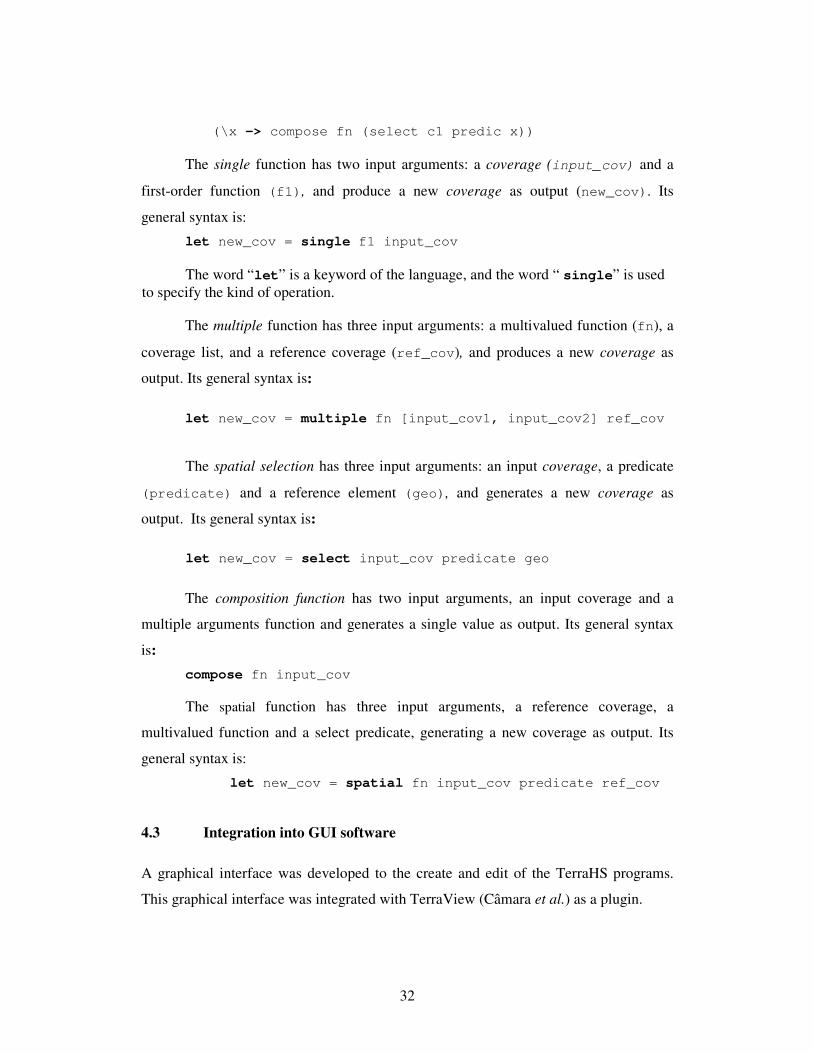
The single function has two input arguments: a coverage (input_cov) and a
first-order function (f1), and produce a new coverage as output (new_cov). Its
general syntax is:
let new_cov = single f1 input_cov
The word “let” is a keyword of the language, and the word “ single” is used to specify the kind of operation.
The multiple function has three input arguments: a multivalued function (fn), a
coverage list, and a reference coverage (ref_cov), and produces a new coverage as
output. Its general syntax is:
let new_cov = multiple fn [input_cov1, input_cov2] ref_cov
The spatial selection has three input arguments: an input coverage, a predicate
(predicate) and a reference element (geo), and generates a new coverage as
output. Its general syntax is:
let new_cov = select input_cov predicate geo
The composition function has two input arguments, an input coverage and a
multiple arguments function and generates a single value as output. Its general syntax
is:
compose fn input_cov
The spatial function has three input arguments, a reference coverage, a
multivalued function and a select predicate, generating a new coverage as output. Its
general syntax is:
let new_cov = spatial fn input_cov predicate ref_cov
4.3 Integration into GUI software
A graphical interface was developed to the create and edit of the TerraHS programs.
This graphical interface was integrated with TerraView (Câmara et al.) as a plugin.

33
4.3.1 Main Window
The main window has a text box that allows the edition of the programs (Figure 4.2).
When the user creates a new program, the text starts with the includes necessaries to
compile and run the Haskell program, and also sets the variables necessaries to the
database connection, according to the database connection opened in the TerraView.
Figure 4.2 – The main window
The interface presents two buttons relatives to the program generation; these
buttons assist the user to insert a coverage and to insert a operation in the program,

34
respectively Insert Coverage and Insert Operation. We also place three buttons to
compile and run a program. The Clear button is used to delete the intermediate files
generated by previous compilation of the program. The Build button is used to compile
the program and to generate an executable file. The RUN button executes the program.
4.3.2 Algebra Interfaces
The sort of windows showed above are used to Insert a Coverage, Insert a Single
Argument Function, Insert a Multiple Argument Function and Insert a Spatial Function.
When we conclude the procedure of insertion, it generates a text of the operation and
insert this text in the text box of the Main Window
• The window of the Figure 4.3 is used to insert a Coverage. To insert a coverage
we select the layer and the attribute; after this we give a name to the coverage.
Figure 4.3 – Insert Coverage
• To insert a single argument function we need to select the output coverage, the
single argument function and the input map (Figure 4.4).

35
Figure 4.4 - Insert Single Argument Function
• To insert a multiple argument function we need to select the output coverage,
the multiple argument function and the list of input coverages (Figure 4.5).
Figure 4.5 - Insert Multiple Arguments Function
• To insert a spatial function we need to select the output coverage, the multiple
argument function, the input coverage, the spatial predicate and the reference
coverage (Figure 4.6).

36
Figure 4.6 – Insert Spatial Function
• When the program is ready we compile it, pressing the “Build Button”. If the
program is correct the Message Box of the Figure 4.7.a will appear, else
Message Box of the figure Figure 4.7.b will appear.
a) b)
Figure 4.7 – Build Windows
• If the program was build with success, to run it we need to press the “Run
button”. If everything is correct the Message Box of the figure Figure 4.8.a) will
appear, else Message Box of the figure Figure 4.8.b) will appear.

37
a) b)
Figure 4.8 – Run Windows
4.4 Examples
The examples use INPE’s database of deforestation of the Brazilian Amazonia (Aguiar,
2006), We selected a data set from the central area of the Pará state, composed of three
coverages: deforestation (grid cells of 25 x 25 km2), roads (lines), and protected areas
(polygons), as shown in Figure 4.9.
Figure 4.9 – Deforestation, protected areas and roads (Pará State, Brazil)
The Figure 4.10 show the main header of the program used for all the programs
of the examples below.

38
module Main(main) where
--import
…
-- db connection
host = "localhost";
dbname = "tedbteste";
user = "root";
password = "";
db = database ( dbname, host, user, password, MySQL )
-- layers and attributes
layer_def = "def_cel"
ldef = layer (db, layer_def)
att_def = attr (ldef , "luc_def")
layer_roads = "roads_lin";
lroads = layer (db, layer_roads)
att_roads = attr (lroads, "object_id_3")
layer_pa = "pa_pol";
lpa = layer (db, layer_pa)
att_pa = attr (lpa, "object_id_1")
-- MAIN
main:: IO ()
main = do
cov_def <- loadMap att_def
cov_roads <- loadMap att_roads
cov_pa <- loadMap att_pa
Figure 4.10 - Main header of the TerraHS programs
We instance the three main coverages of the example:
• cov_def: the deforestation coverage
• cov_roads: the roads
• cov_ap: the protection areas

39
Our first example considers the expression: “Given a coverage of deforestation and
a classification function, return the classified coverage”. The input is the deforestation
coverage and the output is a classified coverage (cov_def_class) The classification
function defines four classes: (1) dense forest; (2) mixed forest with agriculture; (3)
agriculture with forest fragments; (4) agricultural area. This function is:
classify :: Value → Value
classify v
| v < 0.2 = "1"
| ((v > 0.2) && (v < 0.5)) = "2"
| (v > 0.5) && (v < 0.8) = "3"
| v > 0.8 = "4"
We get the classified map (Figure 4.11) using the expression
let cov_def_class = single classify cov_def
Figure 4.11 – Resulting coverage with classified deforestation
As a second example, take the expression: “Calculate the mean deforestation for
each protection area”. The inputs are: the deforestation coverage (cov_def), a spatial
predicate (within), a multivalued function (mean) and the coverage of protected
areas (cov_pa). The output is a coverage of the protected areas (cov_def_prot)
with the same objects as the reference coverage (cov_pa) and the deforestation for
each area.
let cov_def_prot = spatial mean cov_def within cov_ap
40
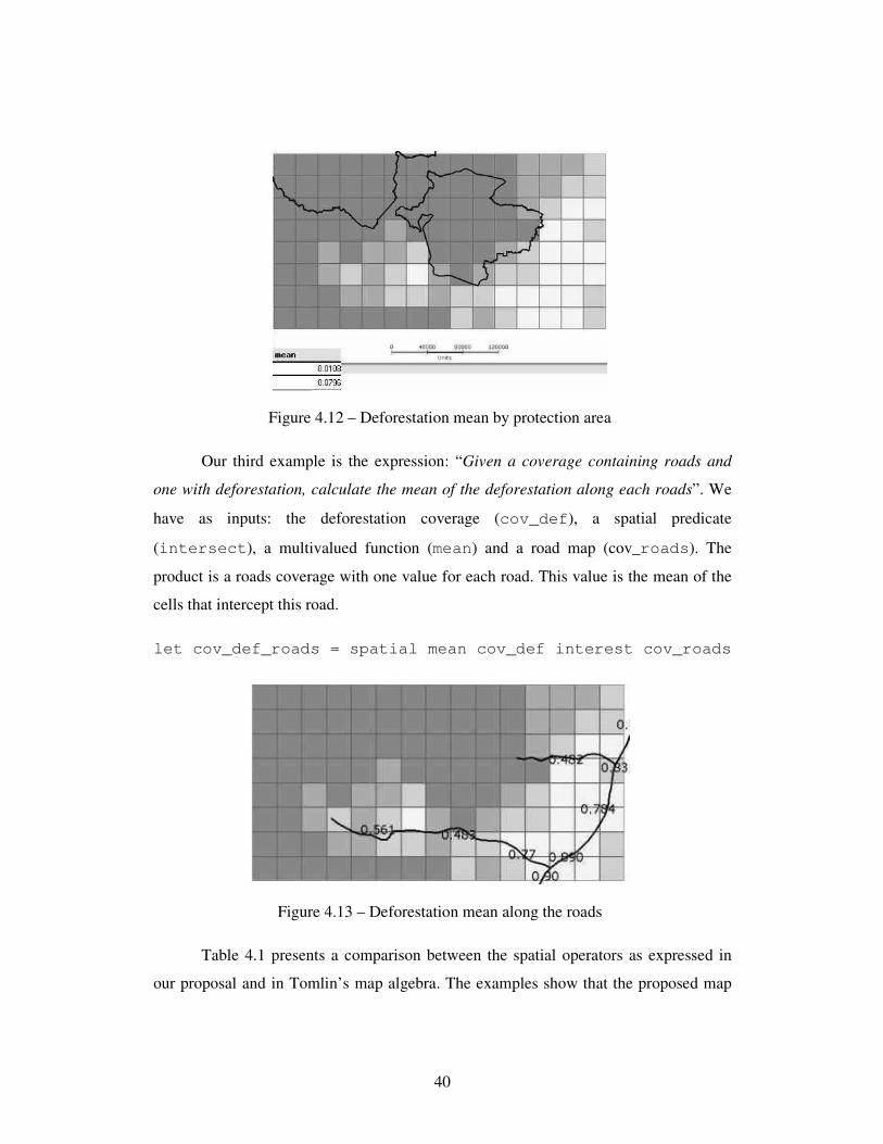
Figure 4.12 – Deforestation mean by protection area
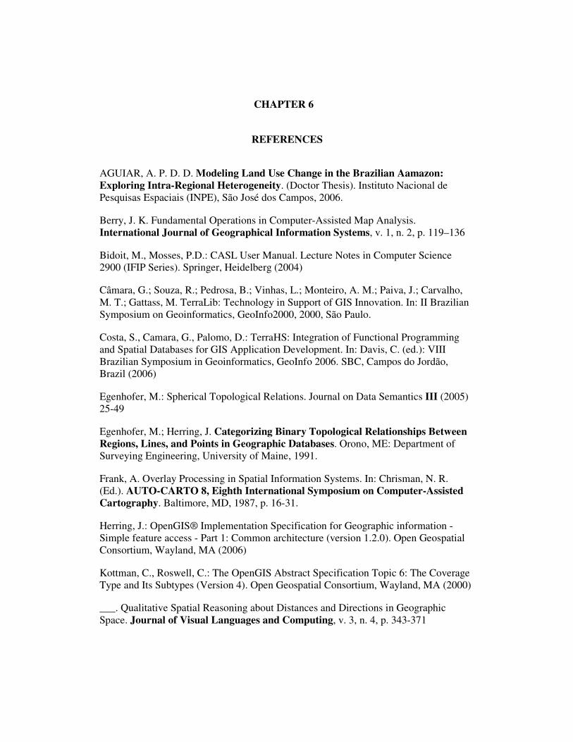
Our third example is the expression: “Given a coverage containing roads and
one with deforestation, calculate the mean of the deforestation along each roads”. We
have as inputs: the deforestation coverage (cov_def), a spatial predicate
(intersect), a multivalued function (mean) and a road map (cov_roads). The
product is a roads coverage with one value for each road. This value is the mean of the
cells that intercept this road.
let cov_def_roads = spatial mean cov_def interest cov_roads
Figure 4.13 – Deforestation mean along the roads
Table 4.1 presents a comparison between the spatial operators as expressed in
our proposal and in Tomlin’s map algebra. The examples show that the proposed map

41
algebra expresses the focal and zonal functions of Tomlin’s map algebra, using the
‘touch’ and ‘within’ topological predicates. Operations involving ‘overlap’,
‘contains’ and ‘intersects’ predicates are part of our proposed coverage algebra
and are not directly expressible by Tomlin’s algebra. This shows that the proposed
algebra is richer than Tomlin’s, as well as having a solid conceptual basis.
Table 4.1 – Comparison of spatial operators with Tomlin’s map algebra
Informal Description Generalized Map Algebra Tomlin
“Focal mean of topography”
fmean:= mean topo
touch fmean
FOCALMEAN OF
TOPOGRAPHY
“Given a coverage of cities and one of topography, find the mean altitude for each city.”
altcit:= mean topo
within city
ZONALMEAN OF
TOPOGRAPHY WITHIN
CITIES
“Given a coverage of national forests, get the deforestation at the edges of each forest”
defBord:= sum defor
overlaps forests
(no equivalent)
“Calculate the mean of the deforestation along the road”
defRoad:= mean defor
intersects road
(no equivalent)

CHAPTER 5
CONCLUSION AND FUTURE WORKS
Map algebra is a fundamental class of operations for spatial data sets. Most of the
current implementations of map algebra use Tomlin’s (Tomlin) proposal for local, focal
and zonal operations. However, Tomlin’s proposal uses ad hoc concepts and lacks a
sound theoretical basis. This work addresses this problem, by proposing a new
foundation for operations involving coverages. We have designed a coverage algebra
that uses topological predicates to express spatial operations and that includes Tomlin’s
algebra as a subset.
There is one important set of operations on coverages that is not part of our
proposal nor of Tomlin’s: convolution operators. A convolution operation requires two
coverages C1 and C2 produces a third coverage C3. The value of each point p of C3 is
the integral of the product of C1 and C2, when C2 is shifted so that its central point is
coincident with p. From a conceptual point of view, convolutions are not part of map
algebra, since the geometrical support for the second coverage C2 (also called a mask)
changes for each point of the output coverage. Convolution does not involve topological
relations, but rather the definition of an integral function.
Our proposal points to a situation where all modeling of topological relations in
two-dimensional spatial datasets can be handled by the 9-intersection model
(dimension-extended), both for simple features and for coverages. Spatial data sets of
higher dimensions (e.g., TIN coverages) need a different foundation. The foundation for
handling spatial relation of higher dimensions requires topological operators that
operate on 3D surfaces (Egenhofer, 2005). Convolution operations are a special case
and need to be handled separately. A possible extension to our algebra would be to
consider directional relations (Frank, 1992), which would be useful to express
operations such as “find the population of all cities north of the river”.

The development of the coverage algebra application using TerraHS in the
Haskell Language enabled it faster, easy and precise implementation. The use of this
implementation in real problems demonstrate the usability of the algebra. Is desirable
that in the future the implementation of coverage algebra can manipulate all the kind of
geographical data available at TerraLib.
Another possible future work is to extend our algebra to the spatiotemporal
domain. Examples of the proposal spatiotemporal algebras are presented in (Güting;
Schneider, 2005), which defines an algebra for moving objects and (Medak, 2001),
which proposes an algebra for modeling change in socio-economical units. To do this
we need to extend the geographical elements of the overage to spatiotemporal domain,
extend our algebra operations and extend the topological predicates to include temporal
predicates.
Even considering the limitations, the expressiveness of the proposed coverage
algebra is considerable. Given that it is based on a solid foundation, it could be
considered as the basis for setting up standard for operations on Open GIS coverages.
The use of standards for operations in coverages would be a significant advance for
increased interoperability of spatial data.
CHAPTER 6
REFERENCES
AGUIAR, A. P. D. D. Modeling Land Use Change in the Brazilian Aamazon: Exploring Intra-Regional Heterogeneity. (Doctor Thesis). Instituto Nacional de Pesquisas Espaciais (INPE), São José dos Campos, 2006.
Berry, J. K. Fundamental Operations in Computer-Assisted Map Analysis. International Journal of Geographical Information Systems, v. 1, n. 2, p. 119–136
Bidoit, M., Mosses, P.D.: CASL User Manual. Lecture Notes in Computer Science 2900 (IFIP Series). Springer, Heidelberg (2004)
Câmara, G.; Souza, R.; Pedrosa, B.; Vinhas, L.; Monteiro, A. M.; Paiva, J.; Carvalho, M. T.; Gattass, M. TerraLib: Technology in Support of GIS Innovation. In: II Brazilian Symposium on Geoinformatics, GeoInfo2000, 2000, São Paulo.
Costa, S., Camara, G., Palomo, D.: TerraHS: Integration of Functional Programming and Spatial Databases for GIS Application Development. In: Davis, C. (ed.): VIII Brazilian Symposium in Geoinformatics, GeoInfo 2006. SBC, Campos do Jordão, Brazil (2006)
Egenhofer, M.: Spherical Topological Relations. Journal on Data Semantics III (2005) 25-49
Egenhofer, M.; Herring, J. Categorizing Binary Topological Relationships Between Regions, Lines, and Points in Geographic Databases. Orono, ME: Department of Surveying Engineering, University of Maine, 1991.
Frank, A. Overlay Processing in Spatial Information Systems. In: Chrisman, N. R. (Ed.). AUTO-CARTO 8, Eighth International Symposium on Computer-Assisted Cartography. Baltimore, MD, 1987, p. 16-31.
Herring, J.: OpenGIS® Implementation Specification for Geographic information - Simple feature access - Part 1: Common architecture (version 1.2.0). Open Geospatial Consortium, Wayland, MA (2006)
Kottman, C., Roswell, C.: The OpenGIS Abstract Specification Topic 6: The Coverage Type and Its Subtypes (Version 4). Open Geospatial Consortium, Wayland, MA (2000)
___. Qualitative Spatial Reasoning about Distances and Directions in Geographic Space. Journal of Visual Languages and Computing, v. 3, n. 4, p. 343-371

___. Higher order functions necessary for spatial theory development. In: Auto-Carto 13, 1997, Seattle, WA. 5: ACSM/ASPRS, p. 11-22.
___. Map Algebra Extended with Functors for Temporal Data. In: Perspectives in Conceptual Modeling: ER 2005 Workshops, 2005, Klagenfurt, Austria. Springer, p. 194-207.
Mennis, J.; Viger, R.; Tomlin, D. Cubic Map Algebra Functions for Spatio-Temporal Analysis. Cartography and Geographic Information Science, v. 32, n. 1, p. 17-32
OGC. OpenGIS Simple Features Specification for SQL. Boston: Open GIS Consortium, 1998.
PEYTON JONES, S. Haskell 98 Language and Libraries the Revised Report 2002.
Peyton Jones, S.; Hughes, J.; Augustsson, L. Haskell 98: A Non-strict, Purely Functional Language. 1999. Disponível em: http://www.haskell.org/onlinereport/.
Pullar, D. MapScript: A Map Algebra Programming Language Incorporating Neighborhood Analysis. GeoInformatica, v. 5, n. 2, p. 145-163
Takeyama, M.; Couclelis, H. Map Dynamics: Integrating Cellular Automata and GIS through Geo-Algebra. International Journal of Geographical Information Systems, v. 11, n. 1, p. 73-91
Thompson, S. Haskell:The Craft of Functional Programming. Harlow, England: Pearson Education, 1999.
Tomlin, C. D. Geographic Information Systems and Cartographic Modeling. Englewood Cliffs, NJ: Prentice-Hall, 1990.
Winter, S. Topological Relations between Discrete Regions. In: Egenhofer, M.; Herring, J. (Ed.). Advances in Spatial Databases—4th International Symposium, SSD ‘95, Portland, ME. Lecture Notes in Computer Science, v. 951. Berlin: Springer-Verlag, 1995, p. 310-327.
Winter, S.; Frank, A. Topology in Raster and Vector Representation. GeoInformatica, v. 4, n. 1, p. 35-65