Embed Size (px)
Citation preview

Policy Research Working Paper 5011
Does the Village Fund Matter in Thailand?Jirawan BoonpermJonathan Haughton
Shahidur R. Khandker
The World BankDevelopment Research GroupSustainable Rural and Urban Development TeamJuly 2009
WPS5011P
ublic
Dis
clos
ure
Aut
horiz
edP
ublic
Dis
clos
ure
Aut
horiz
edP
ublic
Dis
clos
ure
Aut
horiz
edP
ublic
Dis
clos
ure
Aut
horiz
ed

Produced by the Research Support Team
Abstract
The Policy Research Working Paper Series disseminates the findings of work in progress to encourage the exchange of ideas about development issues. An objective of the series is to get the findings out quickly, even if the presentations are less than fully polished. The papers carry the names of the authors and should be cited accordingly. The findings, interpretations, and conclusions expressed in this paper are entirely those of the authors. They do not necessarily represent the views of the International Bank for Reconstruction and Development/World Bank and its affiliated organizations, or those of the Executive Directors of the World Bank or the governments they represent.
Policy Research Working Paper 5011
This paper evaluates the impact of the Thailand Village and Urban Revolving Fund on household expenditure, income, and assets. The revolving fund was launched in 2001 when the Government of Thailand promised to provide a million baht (about $22,500) to every village and urban community in Thailand as working capital for locally-run rotating credit associations. The money —about $2 billion in total—was quickly disbursed to locally-run committees in almost all of Thailand’s 74,000 villages and more than 4,500 urban (including military) communities. By May 2005, the committees had lent a total of about $8 billion, with an average loan of $466.Using data from the Thailand Socioeconomic Surveys of 2002 and 2004, each of which surveys almost 35,000
This paper—a product of the Sustainable Rural and Urban Development Team, Development Research Group—is part of a larger effort in the department to understand the cost-effectiveness of rural financial institutions. Policy Research Working Papers are also posted on the Web at http://econ.worldbank.org. The author may be contacted at [email protected].
households, the authors find that the borrowers were disproportionately poor and agricultural. A propensity score matching model finds that Fund borrowing in 2004 was associated with, on average, 1.9 percent more income, 3.3 percent more expenditure, and about 5 percent more ownership of durable goods. These results are broadly consistent with the results from instrumental variables models (where the identifying instrument was the inverse of village size), which however show a smaller (marginal) effect. Households that borrowed both from the revolving fund and from the Bank of Agriculture and Agricultural Cooperatives gained substantially more in terms of higher income than those who borrowed from either one or the other or from neither.

Does the Village Fund Matter in Thailand?
Jirawan Boonperm National Statistics Office of Thailand, Bangkok
Jonathan Haughton
Suffolk University, Boston
Shahidur R. Khandker World Bank, Washington DC
JEL codes: O16 G21 I38
Note: The authors listed above are in alphabetical order. They would like to thank Chalermkwun Chiemprachanarakorn and her colleagues at the Thai National Statistics Office for helping us work with the Thailand Socioeconomic Survey data, Sheila Buenafe for excellent research assistance and Xiaofei Xu for research support. We are deeply indebted to Kaspar Richter, who was instrumental in adding a special module on the Thailand Village Fund to the 2004 Socioeconomic Survey and arranging for a panel component for that survey. We benefited from comments received from Dean Karlan and Darlene Chisholm, and from participants at a seminar at Suffolk University at a presentation at NEUDC 2007. The views expressed in this paper are those of the authors, and not necessarily of the institutions with which they are affiliated.

Village Fund, draft of June 29, 2009 Page 2 of 34
1. Introduction
In 2001, the government of Thailand launched the Thailand Village and Urban Revolving Fund (VRF)
program, which aimed to provide a million baht (about $22,500) to every village and urban community in
Thailand as working capital for locally-run rotating credit associations.1
Thailand has almost 74,000 villages and over 4,500 urban (including military) communities, so the
total injection of capital into the economy envisaged by the “million baht fund” amounted to 78 billion baht,
equivalent to about $1.75 billion, making it the most ambitious of the estimated 120,000 microfinance
initiatives anywhere in the world.
2
1 The average exchange rate during 2001 was Bht44.51/$, which implies that a million baht are equivalent to $22,468. The exchange rate as of mid-July 2007 was Bht31.23/$, which would value a million baht at $32,020; this is the exchange rate that we use throughout the rest of the paper. 2 Estimated number of microfinance initiatives is from Kaboski and Townsend (2009), p.10.
The program was put into place rapidly. By the end of May 2005 the VRF
committees had lent a total of 259 billion baht ($8.3 billion at the July 2007 exchange rate of Baht 31.23/$) to
17.8 million borrowers (some of whom borrowed more than once). This represents an average loan of $466.
The total repayment of principal amounted to 168 billion baht, leaving outstanding principal of 91 billion
baht.
In this paper we ask a narrowly focused question: Has the VRF had an impact on household
incomes, spending, and asset accumulation, and, if so, how large are these effects? An answer to this
question is necessary, but not sufficient, to help the Government of Thailand determine whether the program
should be expanded or revised, and to help governments of other countries determine whether they should
introduce or expand similar microcredit schemes. In order fully to address these policy issues, one would also
need information on the costs of the program. A complete cost-benefit analysis of the Thailand Village Fund
would be highly desirable, but goes beyond the scope of this paper.
The VRF represents a policy experiment on a grand scale, but it is not the only major source of
household credit, even in rural areas. The Bank for Agriculture and Agricultural Cooperatives (BAAC) has an
extensive network of rural lending. So it is appropriate to ask what additional role the VRF has played, an
issue that we also address in this paper.
We summarize the relevant details of the VRF program in section 2, set out our general approach in
section 3, describe the data employed in the impact evaluation in section 4, and in the subsequent sections
explain the methodology and report the results of the impact evaluation using propensity score matching
(section 5), instrumental variables (section 6), and panel data methods (section 7). The paper ends with a
short set of conclusions in section 8.
Village Fund, draft of June 29, 2009 Page 3 of 34
2. The Thailand Village Revolving Fund
The Thailand Village Revolving Fund became operational very rapidly. Inaugurated in 2001, Village and
Urban Community Fund Committees (henceforth “Village Fund Committees”) had been formed in 92% of
the villages and urban communities in Thailand by 2002, and much of the money had been disbursed. By
May 2005, 99.1% of all villages had a Village Fund in operation and 77.5 billion baht, representing 98.3% of
the originally scheduled amount, had been distributed to Village Fund Committees (Arevart 2005).
Although the initial working capital came from the central government, the Village Funds are locally
run, and have some discretion in setting interest rates, maximum loan amounts, and the terms of loans; some
require, or at least encourage, savings deposits as a condition for borrowing. The Village Fund Committees
process loan applications; households borrow and repay with interest; and the money is lent out again. The
Village Fund Committees do not handle money directly; this is done by a number of intermediaries, of which
the most important are the Government Savings Bank (GSB), which operates mostly in urban areas, and the
Bank for Agriculture and Agricultural Cooperatives (BAAC), which operates only in rural areas and semi-
urban communities.
There are five steps that must be taken in order for a Village Fund to become operational:
(a). The village first sets up a local committee to run the fund and to determine the lending criteria
(interest rate, loan duration, maximum loan size, and objectives).
(b) The properly-established committee then opens an account at the BAAC (which has about 700
branches) or another "facilitator", and the government deposits a million baht into the account.
(c) The local Fund committee sifts through loan applications and determines who may borrow and
under what conditions (interest rate, duration, etc.).
(d) The borrowers go to the BAAC (or other facilitator) to get access to the loans. Each borrower
must open an account – the minimum balance, if it is at the BAAC, is 100 baht – to which their
loan is transferred.
(e) The borrower repays the loan with interest. This requires him or her to visit a BAAC branch
(or that of another facilitator); the borrower typically deposits the repayment directly into the
village fund account. The BAAC provides a regular listing of transactions to each Village Fund.
A number of rules govern the establishment and operating procedures of the committee: three
quarters of the adults in the village must be present at the meeting where it is established; the committee
should have about 15 members, half of them women; while there is some discretion about the amount lent
per loan, it should not generally exceed 20,000 baht and should never exceed 50,000 baht; the loans must
charge a positive interest rate; and it is recommended that loans have at least two guarantors.
The government rates Village Funds on a variety of efficiency and “social” criteria; in any given year,
those that are rated AAA are provided with a “bonus” of a further Bht100,000 to add to their working capital.
Village Fund, draft of June 29, 2009 Page 4 of 34
In addition, Village Funds can borrow an additional million baht (or sometimes just half a million baht, see
below) from the BAAC or other facilitator. The size of this additional loan - i.e. half a million, or a million
baht - is determined by the BAAC using its own (banker's) criteria. Only Village Funds that are ranked 1st
class or 2nd class by BAAC may borrow a million baht; the others (3rd class) may only borrow half a million
baht. The BAAC says that about 1% of these loans are overdue. The BAAC thus rates the managerial
efficiency and potential of VRF Associations and may be intending gradually to withdraw from micro-lending
by giving these village funds a space for competition to run village banks. The BAAC recognizes that Village
Fund Committees generally have an informational advantage in determining who is a good candidate for a
loan.3
3. Measuring the Impact of the Village Revolving Fund
Some of the more dynamic Village Funds are trying to become rural banks, which would potentially
lead to an efficiency gain in that it would allow money to move from one village to another.
The injection of loanable funds due to the VRF was substantial, averaging 2.7% of annual income, or 7.1% of
income for the 38% of households who borrowed. Because a million baht was available for every village,
regardless of size, the importance of the VRF declined with village size: in the smallest tenth of villages, VRF
loans represented 7.9% of income, but just 1.1% of income in the largest decile of villages (Table 1). What
impact might one expect from such a sizeable one-time infusion of cash?
It is not self-evident that an injection of credit into a rural economy will have a measurable impact, or
a positive impact. If financial markets operate well – information is cheap and readily available, there are no
policy distortions – then households should already have access to as much credit as they can productively
use, and they would mainly substitute VRF credit for other sources of credit. So for the VRF to have an
impact on output, it must be predicated on the existence of market imperfections. As a general proposition,
this is not unreasonable, as credit markets have well-known informational asymmetries that in turn can lead
to the inefficient allocation of credit, excessive loan default, monopoly profits for well-informed lenders, and
even credit market collapse (Bardhan and Udry 1999, p.91). The important point is that it cannot be
assumed, a priori, that the VRF will necessarily have a major impact on household welfare.
According to the Socio-Economic Survey undertaken in 2004, 24% of respondent households said
that they did not borrow from the VRF because they had no need for credit, and a further 25% said that they
did not borrow from the VRF because they did not want to take on more debt. We have assumed that in the
absence of general equilibrium effects, the introduction of the VRF credit cannot be expected to have an
3 This process, however, could potentially squeeze out some existing borrowers who may have less access to BAAC loans, and yet not be able to get VRF loans for one reason or another. Moreover, some VRFs may be inefficient for the following reasons: (i) lending to unqualified borrowers; (ii) favoring committee members; (iii) extending loans that are larger than the limit (e.g. 50,000 baht); (iv) not insisting on repayment; (v) charging a lower interest rate; and (vi) landing for longer-than-allowed periods.
Village Fund, draft of June 29, 2009 Page 5 of 34
impact on the incomes or spending patterns of these households; however, this is not an innocuous
assumption, because the very availability of easier credit may reduce the incentive for precautionary (“buffer
stock”) savings, and allow even non-borrowers to spend more than they otherwise would have.
Of those who did borrow, some may not have been credit-constrained, meaning that they had access
to as much credit as they wanted, given the available price. They would then only have taken on VRF loans
because they were cheaper. In part this would produce an income effect – substituting cheap for expensive
credit – but the lower price of credit would also provide an incentive to borrow more overall. The effect
could be large; one in six VRF borrowers said that they borrowed from another source to repay the VRF
loan, and the average annual interest rate paid on those sources was 46.0%; given an average VRF interest
rate of 6.0%, this represents a gain of 40%; given the mean loan size of 16,183 baht, the interest saving would
be equivalent to 4.9% of an average borrowing household’s annual income. While this probably an upper
bound on the cost savings from VRF borrowing, it is enough to allow non-interest consumption for
borrowers to rise by at least 6.1%, with no change in household income.
Other VRF borrowers may have been credit-constrained, in the sense that they already wanted to
borrow more at the available price of credit. Presumably existing lenders were reluctant to lend more due to
prudential concerns, which in turn may have been justified, or may have resulted from asymmetric
information. It is entirely possible that the village-level VRF would, in many cases, have better knowledge
about the ability of village households to service loans than most outside lenders, and thus improve the
efficiency with which credit is allocated.
We do not have direct evidence on whether VRF loans substituted for other credit, or supplemented
other borrowing. Kaboski and Townsend (2009), based on a rural sample of 800 households, find evidence
that in 2003, households took on VRF loans without reducing their other borrowing. This sits well with the
view that many households are credit-constrained, but of course is not inconsistent with the case of non-
constrained households responding to lower borrowing costs.
Much microlending is seen as desirable because it allows households to invest more, and so raise
their earnings, and certainly the VRF was originally viewed as a vehicle for promoting the development of
non-farm enterprise. In this case the impact goes from loan to more investment to more income to more
consumption. On the other hand, many households use credit for consumption purposes – to smooth
consumer spending over the course of a year, or make a lumpy purchases (including durable goods), or
increase consumer spending now relative to in the future. In this case one would observe an increase in
consumer spending without a corresponding rise in income. Given that households are heterogeneous, and
only some would borrow from the VRF for productive purposes, our presumption is that the VRF will have
a stronger impact on consumption spending than on income.
Whether VRF loans were used for investment or for consumer spending, the effect is likely to be
complicated by the fact that a number of credit schemes are already in place. In rural areas, the most
Village Fund, draft of June 29, 2009 Page 6 of 34
important is the Bank for Agriculture and Agricultural Cooperatives (BAAC), which practices individual as
well as group-based lending (mainly to support farming), mobilizes savings as part of financial intermediation,
and is widely considered to be a successful rural finance institution (Yaron 1992, Fitchett 1999). Therefore it
is legitimate to wonder whether the VRF has an added value to rural households that the BAAC could not
provide – are they substitutes or complements? In other words, the relative effectiveness of both programs is
an issue worth examining from the policy point of view, an issue to which we return in section 5.
In short, our main task is to measure the impact of the VRF program on three outcome variables of
interest:
• Expenditure per capita. The measure of expenditure available is based on the Socioeconomic
Surveys of 2002 and 2004, and includes 56 categories of expenditure (and home production),
including the rental value of housing, but does not include the rental value of the household’s durable
goods or vehicles (for lack of data).
• Income per capita. This measure includes 24 categories of income, and includes the rental value of
housing (but not of durable goods).
• A number of measures of household assets, including whether the household has a washing
machine, a VCR, or a motorized vehicle. The SES-2004 did not collect information on the total
value of household assets.
But now we are faced with a methodological problem: VRF borrowers do not represent a random sample of
the households (or adults) surveyed in the Socioeconomic Survey of 2004 – among other things, they are
poorer and more rural.
To get around the problem of non-random assignment, we are obliged to turn to a number of
econometric techniques. These include propensity score matching (section 5) and instrumental variables
(section 6), using data from the Thailand Socioeconomic Surveys of 2002 and 2004. These surveys also
included a panel of rural households, which allows us to estimate the impact of the VRF using double
differences, and instrumental variables with household fixed effects (section 7). But before discussing the
impact evaluation techniques and results, some additional description of the data is in order.
4. The Data
The data for the impact evaluation come from the Thailand Socioeconomic Surveys of 2002 and 2004. The
2004 survey interviewed 34,843 households (covering 116,444 people) throughout the country drawn from
2,044 municipal “blocks” and 1,596 villages in 808 districts. The data were collected in four rounds, spread
throughout the year. The survey collected a wide variety of socio-economic data, including relatively detailed
information on household income and expenditure. It used stratified random sampling with clustering; all the

Village Fund, draft of June 29, 2009 Page 7 of 34
descriptive results presented in this paper apply the appropriate weights (unless otherwise indicated). The
2002 survey used substantially the same questionnaire and covered 34,785 households.
An interesting feature of these two surveys is that they include a panel of 5,755 rural households. An
effort was made in 2004 to re-survey all 6,309 households that had been surveyed in rural areas in rounds 2
and 3 of the 2002 socioeconomic survey. This represents an annual attrition rate of 4.5%, which is relatively
low. A comparison between panel households and those who dropped out of the panel found no appreciable
differences in the relevant variables (in 2002), allaying concerns about attrition bias.
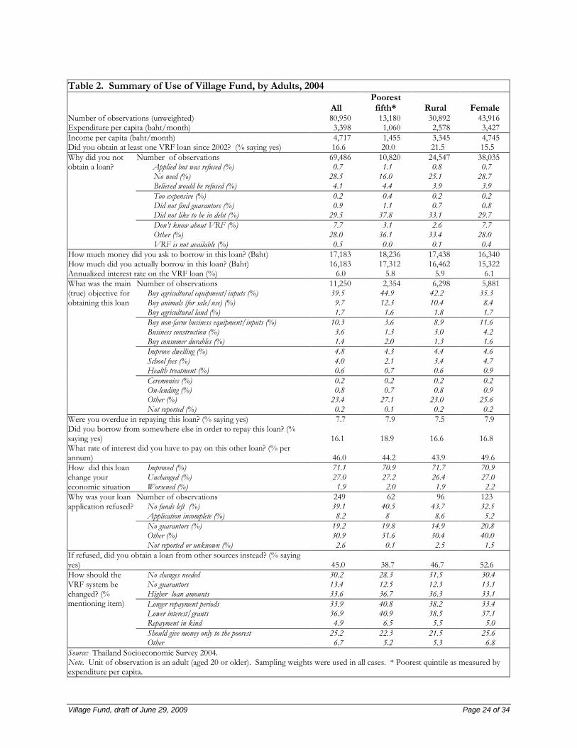
The summary statistics in Table 2 come from a special module that was included in the 2004
socioeconomic survey and that asked all adult members of households about their experience with the VRF.
By 2004, a sixth of all adults had borrowed at least once from the VF, with higher proportions of borrowers
among the poor (defined as those in the poorest quintile, as measured by expenditure per capita) and among
those in rural areas; in this respect, VRF lending differs sharply from the older “village bank” programs in
Northeast Thailand analyzed by Coleman (2002), where the bulk of the loans, and gains, accrued to the
wealthier villagers. Adults in 38 percent of households had borrowed from the VRF by 2004.
Of those adults who did not borrow, less than one percent had been refused a VRF loan, although a
further 4% thought that they would be turned down. On the other hand, over a quarter of non-borrowing
adults said they had no need to borrow, and almost a third said that they did not want to go into debt. Poor
households were less likely to indicate that they did not need to borrow, but more likely to be fearful to going
into debt.
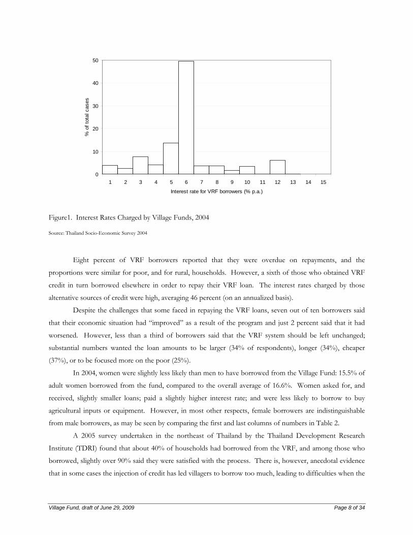
The average amount borrowed in the most recent VRF loan was 16,183 baht (about $518), and this
was only slightly less than the amount requested on average. The mean interest rate charged on VRF loans
was 6.0 percent per year, but there was considerable variation, as Figure 1 shows: substantial numbers of
Village Funds charged annual interest rates of 5, 3, or 12 percent. The interest rate paid by poor, or rural,
borrowers was essentially the same, or perhaps slightly lower, than that paid by other adults.
Although the rhetoric surrounding the Village Revolving Fund program emphasized the importance
of providing finance for processing and packaging, over half of all VRF borrowers said that they planned to
use the money for relatively traditional agricultural purposes. This effect was even more marked among poor
and rural borrowers. Borrowing is fungible, so this does not necessarily imply that spending on agricultural
activities actually rose as a result of the implementation of the Village Fund program, but there is a
dissonance between the reported uses of the borrowed funds and the original aspirations for the Fund.
Village Fund, draft of June 29, 2009 Page 8 of 34
0
10
20
30
40
50
1 2 3 4 5 6 7 8 9 10 11 12 13 14 15
Interest rate for VRF borrowers (% p.a.)
% o
f tot
al c
ases
Figure1. Interest Rates Charged by Village Funds, 2004
Source: Thailand Socio-Economic Survey 2004
Eight percent of VRF borrowers reported that they were overdue on repayments, and the
proportions were similar for poor, and for rural, households. However, a sixth of those who obtained VRF
credit in turn borrowed elsewhere in order to repay their VRF loan. The interest rates charged by those
alternative sources of credit were high, averaging 46 percent (on an annualized basis).
Despite the challenges that some faced in repaying the VRF loans, seven out of ten borrowers said
that their economic situation had “improved” as a result of the program and just 2 percent said that it had
worsened. However, less than a third of borrowers said that the VRF system should be left unchanged;
substantial numbers wanted the loan amounts to be larger (34% of respondents), longer (34%), cheaper
(37%), or to be focused more on the poor (25%).
In 2004, women were slightly less likely than men to have borrowed from the Village Fund: 15.5% of
adult women borrowed from the fund, compared to the overall average of 16.6%. Women asked for, and
received, slightly smaller loans; paid a slightly higher interest rate; and were less likely to borrow to buy
agricultural inputs or equipment. However, in most other respects, female borrowers are indistinguishable
from male borrowers, as may be seen by comparing the first and last columns of numbers in Table 2.
A 2005 survey undertaken in the northeast of Thailand by the Thailand Development Research
Institute (TDRI) found that about 40% of households had borrowed from the VRF, and among those who
borrowed, slightly over 90% said they were satisfied with the process. There is, however, anecdotal evidence
that in some cases the injection of credit has led villagers to borrow too much, leading to difficulties when the
Village Fund, draft of June 29, 2009 Page 9 of 34
funds had to be repaid (Laohong 2006, Gearing 2001). There have also been reports of corruption in the
administration of the VRF in some scores of villages.
The most rigorous study to date of the impact of the VRF uses data from the 2003 and earlier
rounds of a panel of 960 households that Robert Townsend and his colleagues have been following for a
number of years in four provinces of Thailand; 800 households were followed throughout 1997-2003, and
this is the sample used in the study by Kaboski and Townsend (2009). Although the sample size is relatively
small, the survey is rich in detail on household financial assets and transactions. Their most striking finding is
that the proportion of household credit coming from “formal” sources (including the VRF) jumped from
37% in 2001 to 69% in 2002, and was accompanied by little reduction in the use of other credit; in other
words, at least as of 2003, VRF credit supplemented rather than replaced existing sources of credit.
Although the VRF is widely used, and reported levels of satisfaction with it are high, this is no
guarantee that it has had a measurable impact on the outcome variables of interest. Some critics have argued
that many VRF borrowers view the money more as a grant than a loan, in which case it might be expected to
lead to a one-time increase in per capita expenditure and the value of household durables, but not raise
income. Defenders argue that the VRF has had an effect on productivity, raising income and, via higher
income, boosting expenditures. Yet others argue that the main effect of the VRF has been to substitute for
other sources of credit, with very little net impact on real output, spending, or welfare. To determine the
truth in these arguments, a formal impact evaluation is required.
5. Propensity Score Matching
Our first approach to measuring the impact of the VRF is by creating a quasi-experimental design that
matches VRF borrowers with “otherwise identical” non-borrowers, and quantifies any difference in outcome
variables between these two groups. Formally, let
Xi be a vector of pre-treatment covariates (such as age of head of household, location of household,
and so on),
Yi0 be the observed value of the outcome variable (such as expenditure) in the absence of the
treatment,
Yi1 be the observed value of the outcome variable for household i if it has been treated (i.e. it has
borrowed from the VRF), and
Ti be the treatment (equal to 1 if the household is treated, to 0 otherwise).
We want to measure τi ≡ Yi1-Yi0, but this is impossible, because an individual is either in the treatment group
(so be observe Yi1) or the comparison group (so we observe Yi0), but never in both. If we are willing to
assume that households are “assigned” randomly to the treatment group, once we have conditioned on the
covariates, then by a proposition first established by Rubin (1977), the average treatment effect (τ|T=1) is

Village Fund, draft of June 29, 2009 Page 10 of 34
identified and is equal to τ|T=1,X averaged over the distribution of X|Ti=1. In other words, we can measure the
average impact of the VRF by taking each borrower, finding an identical non-borrower (conditioned on the X
covariates), computing the difference in the outcome variable of interest, and taking its mean.
This procedure would only be straightforward if there were just a few covariates; in practice the
problem is more tractable if we can create a summary measure of similarity in the form of a propensity score.
Let p(Xi) be the probability that unit i be assigned to the treatment group, and define
).|()|1Pr()( iiiii XTEXTXp ==≡ (1)
In practice, this probability – the propensity score – could be estimated using a logit or probit equation.
Rosenbaum and Rubin (1983) show that conditional independence extends to the propensity score, so that
treatment cases may be matched with comparison cases using just the propensity score. Furthermore, the
average treatment effect may be obtained by computing the expected value of the difference in the outcome
variable between each treated household and the perfectly matched comparison household (as matched using
the propensity score). Perfect matching is not possible in reality, so in practice one needs to compute
,11|ˆ 1 ∑ ∑∈ ∈
=
−=
Ni Jjj
iiT
i
YJ
YN
τ (2)
where Yi is the observed outcome for the ith individual who is treated and Ji is the set of comparators for i.
The comparators may be chosen with replacement – the approach we take – in which case the bias is lower
but the standard error higher than without replacement. We use single nearest neighbor matching, whereby
one chooses the closest comparator, although other approaches are possible (Abadie et al. 2001); Dehejia and
Wahba (2002) argue that the choice of matching mechanism is not as crucial as the proper estimation of the
propensity scores.
Broadly following an algorithm outlined by Dehejia and Wahba (2002), we first estimated propensity
scores by applying a probit model to a limited number of covariates. We then sorted the observations by
propensity score and divided them into strata sufficiently fine to ensure that there was no statistically
significant difference in propensity scores between treated and non-treated households within each stratum.
We confined this comparison to the area of “common support” – where the propensity scores of the treated
and untreated overlap – and typically needed between 15 and 21 strata. We then checked for the “balancing
property,” which means that within each stratum we tested (using a 1% significance level) whether there was
a difference in the covariates between the treated and non-treated group. Our initial propensity score models
were not well balanced, so we added covariates (including dummy variables for Thailand’s 76 provinces) and
we were able to generate models that were adequately balanced. For instance, when we confined our sample
to rural areas, the propensity score model had 101 covariates, generated 13 strata, and produced 14 cases
where covariates were not balanced. This is acceptable, given that at a one percent level of statistical
significance one would expect to find, erroneously, about 13 cases of imbalance (false negatives).
Village Fund, draft of June 29, 2009 Page 11 of 34
A listing of the variables used in estimating the propensity scores for 2004 is given in Table 3 (except
for the provincial dummy variables). The first thing to note is that on average VRF borrowers are
substantially poorer than those who do not borrow from the VRF, whether measured by monthly
expenditure per capita (2,549 baht vs. 4,286 baht) or income per capita (3,209 baht vs. 6,088 baht), or by
access to subsidized medical care (93% have a 30 baht medical card, vs. 77% for non-borrowers). Compared
to non-borrowers, those who borrow from the VRF are more than twice as likely to be farmers and to be
self-employed, they are more likely to live in the Northeast region, they have larger families, and there are
more earners per household. The important point here is that borrowers differ appreciably from non-
borrowers, at least unless one conditions on the covariates.
The estimate of the probit propensity score equation for the full sample is also shown in Table 3.
The equation fits well enough and, as noted above, appears to be adequately balanced. One of the more
influential variables is the inverse of the number of households per village (or block): The Thai Village Fund
initially provided a fixed amount to every village, irrespective of size, which means that households living in a
large village are less likely to have access to these loans than those in a small village. This effect shows clearly
in the estimates of the propensity score equation reported in Table 3.
Basic Results
Given the propensity scores, it is then possible to match each treatment case with a nearby comparison case,
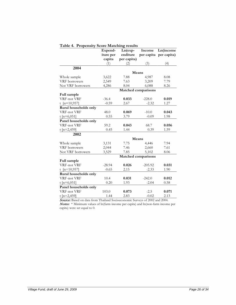
and hence to estimate the impact of VRF borrowing. The results are summarized in Table 4; the upper half
of the table refers to 2004 (with separate propensity score equations for the full sample, for rural households
only, and for the panel), and the bottom half to 2002.
When propensity score matching is used with the full sample of households surveyed in 2004, VRF
borrowing is associated with a statistically significant 3.3% more expenditure per capita and a not-quite-
significant 1.9% higher income per capita. Translated into average increases (at the mean) this implies a rise
in per capita spending of 84 baht per month and of income of 61 baht per month. A reasonable
interpretation is that VRF loans are partly, but not exclusively, functioning as consumer credit; they also
appear to be working through the effect on income. The results based on the 2002 data are comparable: VRF
borrowing is associated with a 3.1% rise in income (t=1.90) and a 2.6% rise in expenditure (t=2.15). To put
these numbers into perspective, the mean size of a VRF loan was 16,183 baht (Table 2), and mean monthly
income per person was 4,987 baht (Table 1) in 2004.
The increases reported in Table 4 are plausible. The boost to income in 2004 represents an
annualized rate of return of 4.5% on the amount borrowed (which averaged 16,183 baht). However, these
effects are only found when expenditure (or income) per capita is shown in log form; when measured in
levels, the VRF has no statistically significant impact in these cases. The use of the log of income (rather than
Village Fund, draft of June 29, 2009 Page 12 of 34
its level) puts more emphasis to increases for poorer households, as the proportional effects (i.e. logs) are
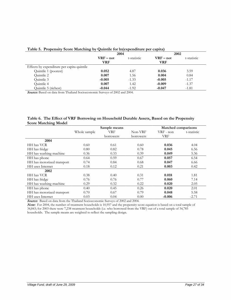
given more weight in these cases. To explore this further, we divided households into quintiles based on the
levels of expenditure per capita, and then applied propensity score matching (with a single nearest neighbor)
to each category. The striking result, shown in Table 5, is that the impact of VRF borrowing is only strong
for the poorest quintile, a finding that holds both for 2002 and 2004. It would thus be appropriate to
categorize the VRF policy as “pro-poor.”
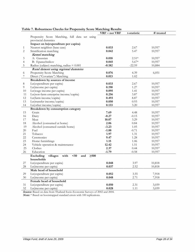
It is instructive to breakdown the impacts further, for each major category of income; the results are
shown in rows 8-14 in Table 7. More VRF borrowing is associated with more farm income (up 49%, albeit
from a modest base of just 522 baht per capita per month) and more income from non-farm enterprises (up
26%). On the other hand, VRF borrowing is not associated with higher wage or transfer income.
One may also break down the impacts by consumer expenditure category (see rows 15-26 in Table
7). There are substantial increases in spending on grain and meat, and also on vehicle operation, although this
last effect is not quite statistically significant. None of the other measured impacts are statistically significant.
These results differ somewhat from those reported by Kaboski and Townsend (2009, Table 5), who found,
for a sample of villages in central Thailand, that VFR credit raised spending on alcohol, and on repairs to
homes and vehicles.
The VRF appears to have the biggest impact in rural areas. If the analysis is repeated for rural
households only, the effect is a statistically significant 6.9% boost to expenditure and 4.3% increase in income
in 2004 (upper panel of Table 4), although the comparable effects in 2002 were much smaller.
There are minimal gender effects. For households that reported having a male head, VRF borrowing
was associated with a 5.2% rise in expenditure and 4.8% increase in income. These figures are only marginally
higher than those for female-headed households, where expenditure rose 5.0% and income by a (non-
significant) 2.8%, as shown in rows 31 and 32 of Table 7.
In addition to the effect on income or expenditure, it might also be expected that VRF borrowing
would have an effect on the accumulation of household assets. It is not possible to measure household gross
or net assets using the Socioeconomic Survey data, but there is a listing of the major physical assets, of which
some of the most important are given in Table 6. There we see, for instance, that 64% of all households
surveyed had a phone in 2004; the rate was 59% for VRF borrowers and 67% for non-borrowers. We then
used our propensity-score matching and found that, for instance, phone ownership among VRF borrowers
was 5.4 percentage points higher than among comparable non-borrowers. Similar effects were found for
VCRs, fridges, washing machines, and motorized transport. This, coupled with the smaller impact on income
than on expenditure, suggests that VRF borrowing was used to some extent in order to get improved access
to consumer and producer durables, despite the fact that fewer than 2% of households reported that this was
the ostensible purpose of their VRF borrowing (see Table 2).
Village Fund, draft of June 29, 2009 Page 13 of 34
Robustness
How robust are these findings? A number of useful checks are summarized in Table 7: row 1 shows the
basic result from Table 4, which is a 3.3% increase in expenditure per capita. Using the same propensity
score equation we first measured the sensitivity of the results to alternative matching methods. Most of the
results are of the same order of magnitude: stratification matching (i.e. matching within broader strata) shows
a 4.2% impact of VRF borrowing on expenditure; kernel matching, which compares the treated case with all
neighbors, but with high weights for near neighbors, shows an impact of between 1.8% (Gaussian kernel) and
4.5% (Epanechnikov kernel). Only caliper matching gives a radically different result – it compares all treated
cases (i.e. VRF borrowers) to those with a propensity score within a radius of 0.001 – indicating, implausibly,
that VRF borrowing reduced expenditure by 18%. This may be because a substantial number of borrowers
with high propensity scores were not matched, and so were excluded, because there were no comparators in
the immediate vicinity. However, this result does lead one to question the assertion by Dehejia and Wahba
(2002) that the choice of matching mechanism is of secondary importance.
A somewhat different check on the robustness of our results is to match treatment households with
non-treatment comparators using direct nearest neighbor matching rather than first estimating propensity
scores. It is not clear that direct (“covariate”) matching represents an improvement, even in principle, over
propensity-score matching, and it is computationally intensive, but if both approaches give similar results then
one can have more confidence in the conclusions. The results, for households living in rural areas (and using
dummy variable for regions, rather than provinces) are shown in rows 6 and 7 of Table 7 and show that while
VRF borrowing is associated with a statistically significant 7.6% increase in per capita spending as measured
using propensity score matching; the effect is much smaller using direct matching – an increase of 1.3% if the
direct match is based on a single nearest neighbor – and not statistically significant.
We also re-estimated the results after deleting villages that were either very small (under 50
households) or rather large (with at least 500 households). Perhaps surprisingly, the results are somewhat
stronger, and show a 4.8% increase in expenditure and 3.7% rise in income due to the VRF (lines 27 and 28
in Table 7).
The most important maintained assumption in propensity score matching is that “the process by
which individuals are assigned or assign themselves to treatment” is ignorable (DiPrete and Gangl 2004). That
is, after removing the effects of observable variables, we may proceed as if subjects were randomly assigned
to treatment. This is a strong assumption. In practice there are likely to be unobserved variables, such as
motivation or ability, that simultaneously affect the outcome, and the assignment to treatment. By definition
we cannot quantify the effects of this “hidden bias”. One solution, proposed by Rosenbaum (2002), is to test
the sensitivity of the results to the introduction of a hypothetical “confounding variable” W, that affects the

Village Fund, draft of June 29, 2009 Page 14 of 34
odds of being assignment to treatment. Let πi be the probability that unit i receives treatment, and Xi the
observed covariates. Then the log odds ratio is given by
ln ( ) , 0 1.1
ii i i
iU Uπ κ γ
π
= + ≤ ≤ − X
Under the hypothesis of ignorability, γ=0 (or equivalently, Γ=1, where Γ≡eγ). With higher values of Γ,
propensity score matching will be less precise. Rosenbaum shows how to obtain significance levels (using a
Wilcoxon sign-rank test) and new confidence intervals (if the treatment effects are additive) for different
values of Γ. The results of estimating these Rosenbaum bounds for the log of expenditure per capita are
shown in Table 8, and show that our results are not especially robust; if an unobserved variable were to cause
the odds ratio of treatment assignment to vary by a factor of about 1.07, then our finding of a impact would
no longer be statistically significant at even the 10% level. Although our results are sensitive to the
assumption of ignorability, this potential loss of significance is, as DiPrete and Gangl (2004) rightly point out,
just a worst-case scenario.
Our final robustness check is to estimate the effect of borrowing on income and consumption using
a common impact model (Haughton and Khandker 2009). Let Yi measure the outcome, Xi be a vector of
covariates, Ti measure the treatment under consideration (i.e. VRF borrowing), and εi represent a zero-mean
error term, and estimate
, 1,..., observations.i C TC i i iY T i nα α β ε= + + + =X
Then the estimate of the coefficient αTC should be able to measure the impact of the borrowing. The results
are shown in Table 9, and use the same other covariates as in the propensity score matching (see Table 3).
When the treatment is measured as a binary variable, set equal to 1 if the household borrows from the VRF,
then the impact is to raise expenditure per capita by 2.3% - broadly in line with the 3.3% impact as measured
using propensity score matching (Table 4); however, the estimated effect on income is nil. One may also
measure the impact of the amount of borrowing, given that one is a borrower. The middle section of Table 8
shows that an additional 100 baht of borrowing is associated with 83 baht more spending and 143 baht more
income, figures that are on the high side, particularly for income, unless “lumpiness” in investment is a
commonly binding constraint. The estimates in the bottom panel of Table 8 imply that a 10% higher loan is
associated with 1.4% more consumption or 1.8% more income, again rather large effects. The common
impact model is less compelling than propensity score matching because it does not confine the estimates to a
region of common support, and does not try to tailor comparisons for each treated case.
Village Fund, draft of June 29, 2009 Page 15 of 34
The Bank for Agriculture and Agricultural Cooperatives
The VRF is not the only, or even necessarily the most important, source of credit for Thai households. The
Bank for Agriculture and Agricultural Cooperatives has an extensive network of rural lending. Of the
households covered by the 2004 socioeconomic survey, 23% borrowed from the VRF only, 15% borrowed
from both the VRF and BAAC, and 6% borrowed from the BAAC only. These figures differ slightly from
those presented earlier because they only refer to the two most important loans incurred by any given
household. But the fact that many households borrow both from the VRF and the BAAC raises the
possibility that our earlier results may be picking up the effect of BAAC borrowing and attributing it to VRF
borrowing.
We therefore applied our propensity score matching approach to borrowing from the BAAC, and
report the results in Table 10. For each comparison (i.e. row in Table 10) we estimated separate propensity-
score equations. From Table 10 it is clear that those who borrowed from the BAAC in 2004 were
comparably poor to, and somewhat more dependent on farm income than, VRF borrowers.
The first point to note is that, based on the results of the propensity-score matching analysis set out
in Table 10, borrowing from the BAAC, with or without other loans, is associated with substantially higher
expenditure per capita (+6.5%) and income per capita (+6.1%). This effect is larger than that of borrowing
from the VRF (expenditure per capita rises 3.3%, income per capita by 1.9%, as shown in Table 4).
The most striking finding is that the combination of borrowing from the BAAC and VRF has
particularly powerful effects, and is associated with 9.1% higher expenditure and 8.5% higher income. Loans
from these two sources appear to be complementary. A plausible interpretation is that many households,
particularly farm households, are credit constrained, even if they borrow from the BAAC; the VRF, by
relaxing these constraints, enables them to boost their incomes. It is noteworthy that borrowing from the
BAAC but not VRF, or from the VRF but not BAAC, has a small and only marginally significant effect on
expenditure levels and an even weaker effect on incomes. This hints at a real, but moderate, degree of
“lumpiness” in investment, where the full return on using borrowed money is only obtained when the sum is
large enough.
The propensity score matching results appear, on balance, to show that VRF borrowing raised
household income and expenditures on average, and that much of the productive effect operated in
agriculture. In the next section we use a different approach, instrumental variables, further to check the
robustness of these results.

Village Fund, draft of June 29, 2009 Page 16 of 34
6. Instrumental Variables
We are interested in finding an unbiased estimate of the impact effect – an estimate of γ – in an outcome
equation of the form
niTY iiii ,...,1,. =+++= εβγα X (3)
where Yi is the outcome of interest, Ti is a dummy variable that equals 1 if the household borrows from the
VRF, and the Xi variables are relevant covariates. However, Ti is a “troublesome explanator” (Murray 2005)
because it is likely correlated with εi: as the basic numbers in Tables 2 and 4 show, VRF borrowers are not a
random sample of the population – they are poorer, spend less, and own fewer durable goods.
An unbiased estimate of γ may be found if one can construct an adequate participation (“first stage”)
equation of the form
),,( iii fT XZ= (4)
where the instruments Zi should be strongly correlated with Ti (“instrumental relevance”) yet be uncorrelated
with εi (“instrument exogeneity”). Then the estimated value, iT̂ , is used in place of iT in equation (3).
We may think of the instrumental variables (IV) estimate of γ as reflecting the “marginal” impact of
the treatment; that is, it measures the impact on expenditure (or income) of one more person borrowing from
the VRF. This differs from the propensity score matching measure, which quantifies the average impact
across all those who are treated. If treatment brings diminishing marginal returns, one might expect the
impact, as measured using propensity score matching, to be larger than that measured using the instrumental
variables approach.
The main practical problem with the IV approach is finding appropriate instruments, yet “the
credibility of IV estimates rests on the arguments offered for the instruments’ validity” (Murray 2005, p.11).
In our case there is one good candidate: the inverse of the size of the village. A feature of the VRF is that it
provided a million baht to each Village Rotating Fund, irrespective of the size of the village. Thus the
probability of obtaining a VRF loan (“participation”) is approximately in inverse proportion to the size of the
village. Our measure of the size of the village is the number of households, which is likely to be closely
correlated with the theoretically ideal measure (the number of people eligible for VRF loans, which is the
number of adults aged 20 and above).
The IV estimates of the impact of the VRF are summarized in Table 11. In each case the first step
equation is probit; an example, for the log of expenditure per capita, is shown in detail in Appendix Table A1.
In all cases the influence of the instrument in the first-stage equations is highly statistically significant, clearly
showing its relevance.
The second-stage equation is linear. Where possible, estimation was done using maximum likelihood
and using sampling weights; in the cases when this estimator did not converge we used a simpler two-step

Village Fund, draft of June 29, 2009 Page 17 of 34
procedure on the unweighted data. In all cases the reported z-statistics have been adjusted to account for the
fact that one is using iT̂ rather than iT in the outcome equation.
The IV results in Table 11, for 2004, show a positive but not statistically significant impact of the
VRF on expenditure and income. In rural areas the measured effects are negative. Curiously, the impact on
farm income, and on non-farm income, are separately large and positive. The results for 2002 show that VRF
borrowing raised expenditure by 9.9%, and income by 8.4%, although the latter effect is not highly
statistically significant.
These results are not particularly robust. The middle rows of Table 11 show the effect on the IV
estimates of adding other instruments. The first instrument is “anydebt”, which equals 1 if the household in
2004 has any outstanding debt. This is strongly correlated with whether a household borrows from the VRF,
but weakly associated with the outcome variable (e.g. simple correlation with expenditure per capita of -0.035;
weighted correlation of -0.109). The inclusion of this instrument raises the measured impact of the VRF to a
statistically significant 16% for income and 20% for expenditure, levels that are certainly on the high end.
It might be objected that “anydebt” is not exogenous, if households borrow from the VRF when
they would not otherwise have borrowed. Alternatively one could use a measure of “non-VRF debt”, set
equal to 1 if the household has debt other than VRF debt. With this instrument the measured impact of VRF
borrowing on household spending rises to an implausible 46%, but even here it might be argued that the new
instrument is not truly exogenous.
Finally, we also add, as an instrument, the interest rate charged by the VRF. It is plausible that a
higher interest rate would deter borrowing – indeed, the weighted correlation coefficient is -0.054 – and be
essentially unrelated to the log of expenditure per capita (correlation of 0.046). The inclusion of this
instrument raises the measure of the impact of VRF borrowing to unrealistically high levels. But it is by no
means a fully satisfactory instrument: when it is included, the sample size falls, because interest-rate
information is only available for villages that have an operating VRF.
In sum, the results of our IV analysis are not very sharp and are partly contradictory. It does seem
reasonable to conclude, however, that the most satisfactory models just use the inverse of the village size as
an instrument; and in this case, the marginal impact of the VRF on expenditure and income is minimal.
Combined with the propensity score matching results, it appears that the VRF raises spending and income on
average, but is experiencing diminishing returns at the margin.
Our results are broadly in line with those found by Kaboski and Townsend (2006), who also used an
instrumental variables approach, but with data from the 2003 and earlier rounds of a panel of 960 households
surveyed in four rural provinces. They checked for robustness by applying a variety of econometric
specifications (levels, changes, and estimates with and without outliers). Their main findings are that greater
use of the VFR was associated with somewhat higher levels of household expenditure, and perhaps an

Village Fund, draft of June 29, 2009 Page 18 of 34
increase in income, and with an increase in agricultural investment as well as spending on fertilizer and
pesticides.
Kaboski and Townsend also found that VRF borrowing was associated with an apparent reduction
in net household assets. This might seem surprising, but could be due to mismeasurement (a farmer might
have invested in drainage or field leveling, and this might not be picked up in survey questions), or because
better access to credit reduces the need to hold assets, or because households overborrowed.
7. Panel Data
An effort was made, in the socioeconomic survey of 2004, to re-survey half of the rural households that had
been interviewed in 2002. This produced a panel of 5,755 rural households for which information is available
for both years. The panel data allow us, in principle, to get a less biased measure of the impact of VRF
borrowing, because one can eliminate unobserved variable bias, provided that the bias is linear and does not
vary over time. It also helps that the introduction of the VRF was a “surprise”, in the sense that it was
proposed and implemented swiftly, and households in 2002 could not easily adjust their behavior in
anticipation of future lending.
Double Differencing
The simplest way to use the panel data is by double differencing. If, before the borrowing, income Yi
depends on covariates Xi, then
,. 0,0,0, tititi caY ε++= X (5)
and afterwards
... 1,1,1, titiiti cTbaY ε+++= X (6)
with .itiit µηε += Differencing gives
.).(. 2,1,0,1,2,1, titititiititi cTbYY µµ −+−+=− XX (7)
Considering those households that did not borrow from the VRF in 2002, a regression of the differenced
outcome variable on the treatment variable (which equals 1 for those who borrowed from the VRF in 2004)
and the change in the covariates should estimate the impact, while “sweeping away” the effects of
unobservable or mismeasured (but time-invariant) covariates. The results of this exercise are shown in the
middle panel of Table 12, which shows little to no impact of the VRF on expenditure (impact of 2.0% but t-
statistic of 1.04), income, or even farm or non-farm income.
To check the robustness of these results, before computing the double differences we first estimated
the propensity scores using the 2002 data and the same variables as in Table 3, and then confined the double

Village Fund, draft of June 29, 2009 Page 19 of 34
differencing to the area of common support. We weighted the differences for each treated case (i.e. VRF
borrower) by 1, and each comparison case by p/(1-p) – where p is the propensity score – as recommended by
Imbens (2004; also Ravallion 2006). The results, shown in the bottom panel of Table 12, were similar to those
of the unweighted, unconstrained estimates: there is a hint of an impact on expenditure per capita, and on
non-farm income per capita, but none of the effects are statistically significant at the conventional levels.
It is also possible to confine the double differencing to those who did not borrow in 2004 (and look
at the effects of borrowing in 2002); or to those who did borrow in 2002 (and look at the effects of
continuing to borrow in 2004).i
None of the results in these cases (not shown here) were statistically
significant.
Panel Instrumental Variables
As a final exercise we undertook an instrumental variables analysis using the (rural) panel data and
incorporating household fixed effects. The linear first-stage equation uses, as instruments, the presence of a
VRF in the village, this measure multiplied by the educational level of the household head, and the size of the
village multiplied by the educational level of the head. The full equations, for the case where the outcome is
the log of expenditure per capita and the comparison is between those who borrowed from the VRF in 2004
and those who borrowed neither in 2002 nor in 2004, are shown in Appendix Table A2.
The key results are summarized in table 13. Households that borrowed from the VRF in 2004 had
15% more income and 18% more expenditure than those who borrowed in neither year, holding other
influences constant; these increases are statistically significant, but also rather large. If, instead, the
comparison is between those who borrowed both in 2002 and 2004 and those who borrowed only in 2004,
the impact of the second year of borrowing was to raise income by 8% and spending by 10%. These
statistically significant rises are within the bounds of plausibility.
8. Conclusions
This study of the impact of the Thailand Village Fund is based entirely on data from the socio-economic
surveys of 2002 and 2004, undertaken just one and three years after the VRF was launched. In the absence of
random assignment, we were obliged to use quasi-experimental methods to quantify the effect of the VRF on
outcome variables. The propensity score matching approach generates reasonable results: the Village
Revolving Fund does appear to have had an impact, raising expenditures by 3.3% and income by 1.9% in
2004. These results are tolerably robust to most specifications of matching, and we may interpret these
numbers as reflecting the average impact of the VRF program.
Village Fund, draft of June 29, 2009 Page 20 of 34
By and large the other results – based on using instrumental variables on cross-section data, double
differences, and instrumental variables using a rural panel – do not contradict the propensity score matching
results. The instrumental variables estimates suggest that the marginal impact of the VRF may be small, even
though, based on the propensity score matching, the average impact is more substantial. The double
difference results show little effect, but the instrumental variables analysis with household fixed effects shows
a surprisingly large impact of VRF borrowing in rural areas.
Our interpretation of these findings is that the VRF has indeed had a moderate impact on household
spending, and also (but to a lesser extent) on household income; this is consistent with our expectations,
based on theory.
Further investigation shows a number of interesting patterns. First, most of the effect of VRF
borrowing is concentrated in the poorest quintile of the population (as measured by expenditure per capita),
where it raised spending by 5.2%, making the program markedly pro-poor. Second, the effect of the VRF
appears to work most convincingly through its influence on farm income, suggesting that it is credit-
constrained farmers who have best been able to put the loans to productive use. This is not what the
designers of the Fund had envisaged; instead they had expected that it would boost household-level non-farm
enterprise (and there is some, if modest, evidence of this too). We speculate that the short-term nature of the
VRF loans makes them suitable for farmers – they allow for the financing of inputs during a crop cycle – but
are not sufficiently long-term (or perhaps large) enough to be very useful for most of the other remunerative
activities that households might initiate.
The third interesting finding is that there are synergies between VRF and BAAC loans; borrowing
from one or the other alone has only a modest discernible impact on incomes or even expenditure, in
contrast to the large impact associated with borrowing from both sources. This has some important practical
implications. The BAAC should be slow to withdraw from village-level lending, even if it is tempted to do so
by a perception that the VRF can fill the gap; or alternatively, the BAAC should be sure to channel enough
resources via the VRF to allow it to fill the gap adequately. Our results also suggest that if the government
wants to expand the VRF, the most productive approach would be to target poorer farming communities.
Finally, a caveat. Our results do not allow one to make a judgment about the desirability of the VRF.
That would require additional information about the full costs of the program and an evaluation of its
sustainability. It would also be valuable to determine whether the impact of the VRF weakens over time, a
finding that is common elsewhere (e.g. Chen et al. 2006; Khandker 2005). These both require further
research, which would be particularly desirable given the importance of the Thai experiment with large-scale
microcredit.

Village Fund, draft of June 29, 2009 Page 21 of 34
References
Abadie, Alberto, David Drukker, Jane Leber Herr and Guido W. Imbens. 2001. “Implementing Matching Estimators for Average Treatment Effects in Stata,” The Stata Journal, 1(1): 1-18.
Arevart, Aupot. 2005. Village and Urban Community Fund Project (VUCFP), Office of the National Village and Urban Community Fund, 31 May.
Bardhan, Pranab and Christopher Udry. 1999. Development Microeconomics, Oxford University Press.
Chen, Shaohua, Ren Mu and Martin Ravallion. 2006. Are there Lasting Impacts of a Poor-Area Development Program? Development Research Group, World Bank, Washington DC.
Coleman, Brett. 2002. Microfinance in Northeast Thailand: Who Benefits and How Much? ERD Working Paper Series No. 9, Asian Development Bank, Manila.
Dehejia, Rajeev H. and Sadek Wahba. 2002. “Propensity Score-Matching Methods for Nonexperimental Causal Studies,” The Review of Economics and Statistics, 84(1): 151-161.
DiPrete, Thomas, and Markus Gangl. 2004. Assessing Bias in the Estimation of Causal Effects: Rosenbaum Bounds on Matching Estimators and Instrumental Variables Estimation with Imperfect Instruments. Unpublished, Department of Sociology, Duke University, Durham NC.
Fitchett, D. 1999. Bank for Agriculture and Agricultural Cooperatives (BAAC), Thailand (Case Study). CGAP, World Bank, Washington DC.
Gearing, Julian. 2001. “The Best Laid Plans …” Asiaweek, March 30.
Haughton, Jonathan and Shahidur Khandker. 2009. Handbook on Poverty and Inequality, World Bank, Washington DC.
Imbens, Guido. 2004. “Nonparametric Estimation of Average Treatment Effects under Exogeneity: A Review,” Review of Economics and Statistics, 86(1): 4-29.
Kaboski, Joseph and Robert Townsend. 2009. The Impacts of Credit on Village Economies. Unpublished, Ohio State University.
Khandker, Shahidur R.. 2005, “Microfinance and poverty: An Analysis using Panel Household Survey Data from Bangladesh” World Bank Economic Review.
Laohong, Ging-or. Laohong. 2005. “Thailand: Gov’t Million Dollar Funds Lead Villagers to Poverty,” Writing For Peace, http://www.ipsnewsasia.net/writingpeace/index.html . June 5. [Accessed July 13, 2006].
Murray, Michael. 2005. The Bad, the Weak, and the Ugly: Avoiding the Pitfalls of Instrumental Variables Estimation. Bates College. Unpublished.
Ravallion, Martin. 2006. Evaluating Anti-Poverty Programs. For Robert Evenson and T. Paul Schultz (eds.), Handbook of Development Economics, Vol. 4, North Holland, Amsterdam.
Rosenbaum, Paul. 2002. Observational Studies, 2nd edition. Springer, New York.
Rosenbaum, P. and D. Rubin. 1983. “The Central Role of the Propensity Score in Observational Studies for Causal Effects,” Biometrika, 70(1): 41-55. April.
Rubin, D. 1977. “Assignment to a Treatment Group on the Basis of a Covariate,” Journal of Educational Statistics, 2(1): 1-26. Spring.

Village Fund, draft of June 29, 2009 Page 22 of 34
Townsend, Robert M. 2006, The Thai Economy: Growth, Inequality, Poverty and the Evaluation of Financial Systems, draft. Chapter 8: “Impacts: Experimental and Econometric Program Evaluations.”
Yaron, J. 1992. Successful Rural Finance Institutions. World Bank Discussion Paper 150, Washington, DC.

Village Fund, draft of June 29, 2009 Page 23 of 34
Table 1. Village Rotating Fund Lending by Village Size
Income in 2004, baht per month Average VRF loan/income
% of households borrowing from VRF Decile # of households Per capita Per household
1 75 3,588 12,975 7.9 63.6 2 103 4,163 14,450 4.6 49.3 3 119 5,342 18,836 2.5 37.0 4 133 5,012 17,145 2.6 37.8 5 147 5,431 18,537 2.1 35.7 6 163 5,317 18,312 2.1 34.6 7 183 5,006 17,385 2.1 35.7 8 211 4,966 16,889 2.1 35.6 9 256 5,071 17,487 1.7 30.5 10 368 6,120 20,020 1.1 21.3
Total 175 4,987 17,198 2.7 38.2 Source: From Thailand Socio-Economic Survey of 2004.
Village Fund, draft of June 29, 2009 Page 24 of 34
Table 2. Summary of Use of Village Fund, by Adults, 2004
All Poorest fifth* Rural Female
Number of observations (unweighted) 80,950 13,180 30,892 43,916 Expenditure per capita (baht/month) 3,398 1,060 2,578 3,427 Income per capita (baht/month) 4,717 1,455 3,345 4,745 Did you obtain at least one VRF loan since 2002? (% saying yes) 16.6 20.0 21.5 15.5 Why did you not obtain a loan?
Number of observations 69,486 10,820 24,547 38,035 Applied but was refused (%) 0.7 1.1 0.8 0.7 No need (%) 28.5 16.0 25.1 28.7 Believed would be refused (%) 4.1 4.4 3.9 3.9 Too expensive (%) 0.2 0.4 0.2 0.2 Did not find guarantors (%) 0.9 1.1 0.7 0.8 Did not like to be in debt (%) 29.5 37.8 33.1 29.7 Don’t know about VRF (%) 7.7 3.1 2.6 7.7 Other (%) 28.0 36.1 33.4 28.0 VRF is not available (%) 0.5 0.0 0.1 0.4
How much money did you ask to borrow in this loan? (Baht) 17,183 18,236 17,438 16,340 How much did you actually borrow in this loan? (Baht) 16,183 17,312 16,462 15,322 Annualized interest rate on the VRF loan (%) 6.0 5.8 5.9 6.1 What was the main (true) objective for obtaining this loan
Number of observations 11,250 2,354 6,298 5,881 Buy agricultural equipment/inputs (%) 39.5 44.9 42.2 35.3 Buy animals (for sale/use) (%) 9.7 12.3 10.4 8.4 Buy agricultural land (%) 1.7 1.6 1.8 1.7 Buy non-farm business equipment/inputs (%) 10.3 3.6 8.9 11.6 Business construction (%) 3.6 1.3 3.0 4.2 Buy consumer durables (%) 1.4 2.0 1.3 1.6 Improve dwelling (%) 4.8 4.3 4.4 4.6 School fees (%) 4.0 2.1 3.4 4.7 Health treatment (%) 0.6 0.7 0.6 0.9 Ceremonies (%) 0.2 0.2 0.2 0.2 On-lending (%) 0.8 0.7 0.8 0.9 Other (%) 23.4 27.1 23.0 25.6 Not reported (%) 0.2 0.1 0.2 0.2
Were you overdue in repaying this loan? (% saying yes) 7.7 7.9 7.5 7.9 Did you borrow from somewhere else in order to repay this loan? (% saying yes) 16.1 18.9 16.6 16.8 What rate of interest did you have to pay on this other loan? (% per annum) 46.0 44.2 43.9 49.6 How did this loan change your economic situation
Improved (%) 71.1 70.9 71.7 70.9 Unchanged (%) 27.0 27.2 26.4 27.0 Worsened (%) 1.9 2.0 1.9 2.2
Why was your loan application refused?
Number of observations 249 62 96 123 No funds left (%) 39.1 40.5 43.7 32.5 Application incomplete (%) 8.2 8 8.6 5.2 No guarantors (%) 19.2 19.8 14.9 20.8 Other (%) 30.9 31.6 30.4 40.0 Not reported or unknown (%) 2.6 0.1 2.5 1.5
If refused, did you obtain a loan from other sources instead? (% saying yes) 45.0 38.7 46.7 52.6 How should the VRF system be changed? (% mentioning item)
No changes needed 30.2 28.3 31.5 30.4 No guarantors 13.4 12.5 12.3 13.1 Higher loan amounts 33.6 36.7 36.3 33.1 Longer repayment periods 33.9 40.8 38.2 33.4 Lower interest/grants 36.9 40.9 38.5 37.1 Repayment in kind 4.9 6.5 5.5 5.0 Should give money only to the poorest 25.2 22.3 21.5 25.6 Other 6.7 5.2 5.3 6.8
Source: Thailand Socioeconomic Survey 2004. Note. Unit of observation is an adult (aged 20 or older). Sampling weights were used in all cases. * Poorest quintile as measured by expenditure per capita.

Village Fund, draft of June 29, 2009 Page 25 of 34
Table 3. Summary of Variables Used in Propensity Score Analysis for 2004
Full sample VRF borrowers Propensity Score
Equation
Mean Std. Dev. Mean
Std. Dev. Coefficient p-value
Does household borrow from VRF? (Yes=1) 0.38 0.49 1.00 - Age of head (in years) 49.67 14.84 50.37 13.16 0.017 0.00 Educational level of head (in years) 7.09 4.39 6.09 3.18 0.100 0.00 Head of household is male (yes=1) 0.70 0.46 0.74 0.44 -0.048 0.05 Number of adult males in household 1.09 0.71 1.17 0.71 -0.153 0.00 Number of adult females in household 1.27 0.70 1.33 0.63 -0.136 0.00 Number of males working in agriculture 0.45 0.65 0.68 0.70 -0.042 0.42 Number of males working in industry 0.20 0.46 0.17 0.43 -0.113 0.03 Number of males working in trade 0.13 0.39 0.10 0.34 -0.241 0.00 Number of males working in services 0.20 0.44 0.15 0.39 -0.095 0.07 Number of females working in agriculture 0.44 0.60 0.69 0.64 0.053 0.30 Number of females working in industry 0.17 0.42 0.15 0.39 -0.118 0.02 Number of females working in trade 0.13 0.39 0.11 0.35 -0.196 0.00 Number of females working in services 0.21 0.48 0.15 0.39 -0.127 0.01 Municipal area (yes=1) 0.33 0.47 0.12 0.33 -0.452 0.00 Province 1 (metro Bangkok) -0.660 0.00 province2 -0.238 0.06 province3 -0.173 0.154 … Age of household head (in years ’00), squared 2,688 1,556 2,710 1,381 -1.935 0.00 Educational level of head (in years), squared 69.55 83.77 47.18 54.97 -0.006 0.00 One-person household 0.10 0.31 0.04 0.20 -0.257 0.00 Household with two parents 0.67 0.47 0.75 0.43 0.097 0.00 Household with one parent 0.10 0.30 0.09 0.29 -0.074 0.03 Household has 30 baht medical card 0.83 0.38 0.93 0.26 0.223 0.00 Household gets lunch or food subsidy 0.24 0.43 0.34 0.48 0.068 0.00 Size of household 3.45 1.66 3.84 1.61 0.100 0.00 Head of household is self-employed 0.48 0.50 0.65 0.48 -2.146 0.00 Head of household is an employee 0.34 0.47 0.23 0.42 -2.351 0.00 Head of household has another employment 0.18 0.39 0.12 0.33 -2.211 0.00 Number of earners in household 1.94 1.07 2.21 1.03 0.247 0.00 1/(number of households per village or block) 0.00694 0.0031 0.00775 0.0034 29.810 0.00 Constant 0.395 0.57 Memo: Outcome variables Household current income, baht/capita per mth 4,987 7,119 3,209 3,385 Pseudo R2 0.190 Household consumption, baht/capita per mth 3,622 4,190 2,549 2,410 Region of
common support
0.004 to 0.985 Household farm income, baht/capita per month 522 1,809 785 2,048
Household non-farm income, baht/capita per mth 3,964 6,780 2,065 2,855 Percentage rise in income since 2002 0.55 15.09 0.32 16.32 Number of observations 34,843 10,985 34,752 Source: Thailand socioeconomic survey, 2004. Note: Means are weighted to take structure of sampling into account.
Village Fund, draft of June 29, 2009 Page 26 of 34
Table 4. Propensity Score Matching results Expend-
iture per capita
Ln(exp-enditure
per capita)
Income per capita
Ln(income per capita)
(1) (2) (3) (4) 2004
Means Whole sample 3,622 7.88 4,987 8.08 VRF borrowers 2,549 7.63 3,209 7.79 Not VRF borrowers 4,286 8.04 6,088 8.26 Matched comparisons Full sample VRF-not VRF -36.4 0.033 -228.0 0.019 t [n=10,957] -0.59 2.67 -2.32 1.27 Rural households only VRF-not VRF 48.0 0.069 -10.0 0.043 t [n=6,051] 0.55 3.79 -0.09 1.98 Panel households only VRF-not VRF 59.2 0.043 68.7 0.056 t [n=2,459] 0.45 1.44 0.39 1.59
2002 Means Whole sample 3,131 7.75 4,446 7.94 VRF borrowers 2,044 7.46 2,660 7.61 Not VRF borrowers 3,529 7.85 5,102 8.06 Matched comparisons Full sample VRF-not VRF -28.94 0.026 -205.92 0.031 t [n=10,957] -0.65 2.15 -2.33 1.90 Rural households only VRF-not VRF 10.4 0.031 -242.0 0.012 t [n=6,051] 0.20 1.93 -2.04 0.58 Panel households only VRF-not VRF 103.0 0.073 -2.5 0.071 t [n=2,459] 1.44 2.83 -0.02 2.13 Source: Based on data from Thailand Socioeconomic Surveys of 2002 and 2004. Notes: * Minimum values of ln(farm income per capita) and ln(non-farm income per capita) were set equal to 0.
Village Fund, draft of June 29, 2009 Page 27 of 34
Table 5. Propensity Score Matching by Quintile for ln(expenditure per capita) 2004 2002 VRF – not
VRF t-statistic VRF – not
VRF t-statistic
Effects by expenditure per capita quintile Quintile 1 (poorest) 0.052 4.87 0.036 3.59 Quintile 2 0.007 1.56 0.004 0.84 Quintile 3 -0.005 -1.33 -0.005 -1.17 Quintile 4 0.007 1.42 -0.009 -1.37 Quintile 5 (richest) -0.044 -1.92 -0.047 -1.81
Source: Based on data from Thailand Socioeconomic Surveys of 2002 and 2004.
Table 6. The Effect of VRF Borrowing on Household Durable Assets, Based on the Propensity Score Matching Model Sample means Matched comparisons
Whole sample VRF borrowers
Non-VRF borrowers
VRF - non VRF
t-statistic
2004 HH has VCR 0.60 0.61 0.60 0.036 4.04 HH has fridge 0.80 0.82 0.78 0.045 6.56 HH has washing machine 0.36 0.33 0.39 0.049 5.36 HH has phone 0.64 0.59 0.67 0.057 6.54 HH has motorized transport 0.74 0.84 0.68 0.047 6.66 HH uses Internet 0.18 0.12 0.21 0.003 0.42
2002 HH has VCR 0.38 0.40 0.31 0.018 1.81 HH has fridge 0.76 0.76 0.77 0.060 7.14 HH has washing machine 0.29 0.32 0.22 0.020 2.05 HH has phone 0.40 0.45 0.26 0.020 2.01 HH has motorized transport 0.70 0.67 0.79 0.048 5.58 HH uses Internet 0.03 0.04 0.00 -0.006 -2.71 Source: Based on data from the Thailand Socioeconomic Surveys of 2002 and 2004. Note: For 2004, the number of treatment households is 10,957 and the propensity score equation is based on a total sample of 34,843; for 2003 there were 7,238 treatment households (i.e. who borrowed from the VRF) out of a total sample of 34,785 households. The sample means are weighted to reflect the sampling design.
Village Fund, draft of June 29, 2009 Page 28 of 34
Table 7. Robustness Checks for Propensity Score Matching Results
VRF – not VRF t-statistic # treated Propensity Score Matching, full data set using
provincial dummies
Impact on ln(expenditure per capita) 1 Nearest neighbor (base case) 0.033 2.67 10,957 2 Stratification matching 0.042 5.47 10,957
Kernel matching 3 A: Gaussian 0.018 2.51* 10,957 4 B: Epanechnikov 0.045 5.67* 10,957 5 Radius (caliper) matching, radius = 0.001 -0.182 -22.59 10,884 Rural dataset using regional dummies 6 Propensity Score Matching 0.076 4.39 6,051 7 Direct (“Covariate”) Matching 0.013 1.02
Breakdown by sources of income 8 Ln(expenditure per capita) 0.033 2.67 10,957 9 Ln(income per capita) 0.190 1.27 10,957 10 Ln(wage income per capita) 0.095 1.41 10,957 11 Ln(non-farm enterprise income/capita) 0.256 3.87 10,957 12 Ln(farm income/capita) 0.493 8.87 10,957 13 Ln(transfer income/capita) 0.050 0.93 10,957 14 Ln(other income/capita) 0.133 3.20 10,957
Breakdown by consumption category 15 Grain 7.69 4.48 10,957 16 Dairy -0.27 -0.15 10,957 17 Meat 10.07 3.29 10,957 18 Alcohol (consumed at home) 2.06 0.84 10,957 19 Alcohol (consumed outside home) -3.23 1.05 10,957 20 Fuel -1.88 -0.71 10,957 21 Tobacco 1.97 1.31 10,957 22 Ceremonies 9.47 1.28 10,957 23 Home furnishings 1.15 1.06 10,957 24 Vehicle operation & maintenance 12.42 1.51 10,957 25 Clothes 2.37 0.44 10,957 26 Education -1.79 -0.58 10,957 Excluding villages with <50 and ≥500
households
27 Ln(expenditure per capita) 0.048 3.97 10,818 28 Ln(income per capita) 0.037 2.52 10,818 Male head of household 29 Ln(expenditure per capita) 0.052 3.55 7,918 30 Ln(income per capita) 0.048 2.71 7,918 Female head of household 31 Ln(expenditure per capita) 0.050 2.31 3,039 32 Ln(income per capita) 0.028 1.11 3,039 Source: Based on data from Thailand Socio-Economic Surveys of 2002 and 2004. Note: * Based on bootstrapped standard errors with 100 replications.
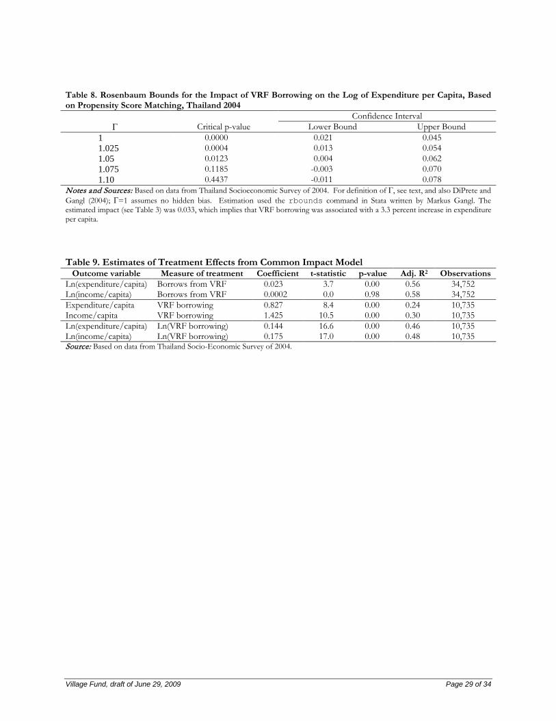
Village Fund, draft of June 29, 2009 Page 29 of 34
Table 8. Rosenbaum Bounds for the Impact of VRF Borrowing on the Log of Expenditure per Capita, Based on Propensity Score Matching, Thailand 2004
Confidence Interval Γ Critical p-value Lower Bound Upper Bound
1 0.0000 0.021 0.045 1.025 0.0004 0.013 0.054 1.05 0.0123 0.004 0.062 1.075 0.1185 -0.003 0.070 1.10 0.4437 -0.011 0.078
Notes and Sources: Based on data from Thailand Socioeconomic Survey of 2004. For definition of Γ, see text, and also DiPrete and Gangl (2004); Γ=1 assumes no hidden bias. Estimation used the rbounds command in Stata written by Markus Gangl. The estimated impact (see Table 3) was 0.033, which implies that VRF borrowing was associated with a 3.3 percent increase in expenditure per capita. Table 9. Estimates of Treatment Effects from Common Impact Model
Outcome variable Measure of treatment Coefficient t-statistic p-value Adj. R2 Observations Ln(expenditure/capita) Borrows from VRF 0.023 3.7 0.00 0.56 34,752 Ln(income/capita) Borrows from VRF 0.0002 0.0 0.98 0.58 34,752 Expenditure/capita VRF borrowing 0.827 8.4 0.00 0.24 10,735 Income/capita VRF borrowing 1.425 10.5 0.00 0.30 10,735 Ln(expenditure/capita) Ln(VRF borrowing) 0.144 16.6 0.00 0.46 10,735 Ln(income/capita) Ln(VRF borrowing) 0.175 17.0 0.00 0.48 10,735 Source: Based on data from Thailand Socio-Economic Survey of 2004.

Village Fund, draft of June 29, 2009 Page 30 of 34
Table 10. Propensity Score Matching Results for BAAC vs. VRF
2004
Expenditure per capita
Income per capita
# obser-vations
(unweighted) Level Log Level Log (1) (2) (3) (4) (7) Means
Whole sample 3,622 7.88 4,987 8.08 34,843 Borrow from VRF 2,549 7.63 3,209 7.79 10,985 Borrow from VRF but not BAAC 2,724 7.68 3,396 7.83 7,268 Borrow from BAAC 2,378 7.58 3,107 7.75 5,624 Borrow from BAAC but not VRF 2,656 7.66 3,463 7.82 2,854 Borrow from BAAC and VRF 2,292 7.56 2,934 7.73 3,717 Borrow from neither VRF nor BAAC 4,486 8.09 6,390 8.31 21,951
Matched Comparisons Level Log Level Log
Borrow from BAAC (and possibly others) BAAC-not BAAC 124.16 0.065 25.79 0.061 34,843 t-statistic 1.88 4.46 0.22 3.40 Borrow from BAAC (but not from VRF) BAAC-not BAAC 45.95 0.036 -29.01 0.038 34,843 t-statistic 0.41 1.63 -0.14 1.40 Borrow from VRF (but not from BAAC) VRF-not VRF 9.38 0.021 -98.67 0.015 34,843 t-statistic 0.15 1.67 -1.05 0.97 Borrow from TVC and BAAC BAAC+VRF-not BAAC or VRF 190.4 0.091 150.2 0.085 34,843 t-statistic 3.0 5.8 1.8 4.5
2002
Expenditure per capita
Income per capita
# observations
Level Log Level Log Means
Whole sample 3,130 7.75 4,446 7.94 34,785 Borrow from VRF 2,044 7.46 2,660 7.60 7,243 Borrow from VRF but not BAAC 2,111 2.48 2,733 7.62 4,760 Borrow from BAAC 2,018 7.43 2,724 7.59 5,326 Borrow from BAAC but not VRF 2,098 7.44 2,911 7.61 2,843 Borrow from BAAC and VRF 1,942 7.43 2,547 7.58 2,483 Borrow from neither VRF nor BAAC 4,486 8.09 6,390 8.31 21,951
Matched Comparisons Level Log Level Log
Borrow from BAAC (and possibly others) BAAC-not BAAC 125.79 0.061 131.11 0.098 34,785 t-statistic 2.68 4.42 1.06 5.26 Borrow from BAAC (but not from VRF) BAAC-not BAAC 112.12 0.043 99.10 0.057 34,785 t-statistic 1.84 2.54 0.59 2.49 Borrow from VRF (but not from BAAC) VRF-not VRF -178.54 -0.027 -378.17 -0.028 34,785 t-statistic 3.37 -1.97 -3.15 -1.57 Borrow from TVC and BAAC BAAC+VRF-not BAAC or VRF 122.9 0.071 8.6 0.077 34,785 t-statistic 2.3 4.2 0.1 3.3 Source: Based on data from Thailand Socioeconomic Surveys of 2002 and 2004. Notes: * Minimum value of ln(farm income per capita) and ln(non-farm income per capita) set equal to 0 in all cases. All the propensity score equations use dummy variables for the provinces, as well as the other variables
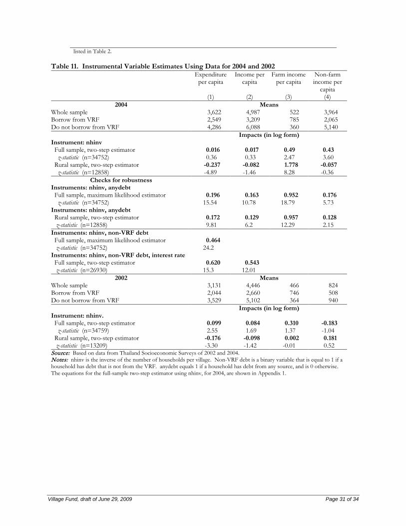
Village Fund, draft of June 29, 2009 Page 31 of 34
listed in Table 2. Table 11. Instrumental Variable Estimates Using Data for 2004 and 2002
Expenditure per capita
Income per capita
Farm income per capita
Non-farm income per
capita (1) (2) (3) (4)
2004 Means Whole sample 3,622 4,987 522 3,964 Borrow from VRF 2,549 3,209 785 2,065 Do not borrow from VRF 4,286 6,088 360 5,140
Impacts (in log form) Instrument: nhinv Full sample, two-step estimator 0.016 0.017 0.49 0.43 z-statistic (n=34752) 0.36 0.33 2.47 3.60 Rural sample, two-step estimator -0.237 -0.082 1.778 -0.057 z-statistic (n=12858) -4.89 -1.46 8.28 -0.36
Checks for robustness Instruments: nhinv, anydebt Full sample, maximum likelihood estimator 0.196 0.163 0.952 0.176 z-statistic (n=34752) 15.54 10.78 18.79 5.73 Instruments: nhinv, anydebt Rural sample, two-step estimator 0.172 0.129 0.957 0.128 z-statistic (n=12858) 9.81 6.2 12.29 2.15 Instruments: nhinv, non-VRF debt Full sample, maximum likelihood estimator 0.464 z-statistic (n=34752) 24.2 Instruments: nhinv, non-VRF debt, interest rate Full sample, two-step estimator 0.620 0.543 z-statistic (n=26930) 15.3 12.01
2002 Means Whole sample 3,131 4,446 466 824 Borrow from VRF 2,044 2,660 746 508 Do not borrow from VRF 3,529 5,102 364 940
Impacts (in log form) Instrument: nhinv. Full sample, two-step estimator 0.099 0.084 0.310 -0.183 z-statistic (n=34759) 2.55 1.69 1.37 -1.04 Rural sample, two-step estimator -0.176 -0.098 0.002 0.181 z-statistic (n=13209) -3.30 -1.42 -0.01 0.52 Source: Based on data from Thailand Socioeconomic Surveys of 2002 and 2004. Notes: nhinv is the inverse of the number of households per village. Non-VRF debt is a binary variable that is equal to 1 if a household has debt that is not from the VRF. anydebt equals 1 if a household has debt from any source, and is 0 otherwise. The equations for the full-sample two-step estimator using nhinv, for 2004, are shown in Appendix 1.
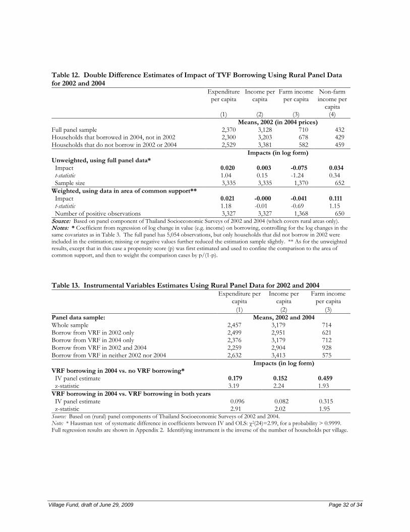
Village Fund, draft of June 29, 2009 Page 32 of 34
Table 12. Double Difference Estimates of Impact of TVF Borrowing Using Rural Panel Data for 2002 and 2004
Expenditure per capita
Income per capita
Farm income per capita
Non-farm income per
capita (1) (2) (3) (4) Means, 2002 (in 2004 prices)
Full panel sample 2,370 3,128 710 432 Households that borrowed in 2004, not in 2002 2,300 3,203 678 429 Households that do not borrow in 2002 or 2004 2,529 3,381 582 459
Impacts (in log form) Unweighted, using full panel data* Impact 0.020 0.003 -0.075 0.034 t-statistic 1.04 0.15 -1.24 0.34 Sample size 3,335 3,335 1,370 652 Weighted, using data in area of common support** Impact 0.021 -0.000 -0.041 0.111 t-statistic 1.18 -0.01 -0.69 1.15 Number of positive observations 3,327 3,327 1,368 650 Source: Based on panel component of Thailand Socioeconomic Surveys of 2002 and 2004 (which covers rural areas only). Notes: * Coefficient from regression of log change in value (e.g. income) on borrowing, controlling for the log changes in the same covariates as in Table 3. The full panel has 5,054 observations, but only households that did not borrow in 2002 were included in the estimation; missing or negative values further reduced the estimation sample slightly. ** As for the unweighted results, except that in this case a propensity score (p) was first estimated and used to confine the comparison to the area of common support, and then to weight the comparison cases by p/(1-p).
Table 13. Instrumental Variables Estimates Using Rural Panel Data for 2002 and 2004
Expenditure per capita
Income per capita
Farm income per capita
(1) (2) (3) Panel data sample: Means, 2002 and 2004 Whole sample 2,457 3,179 714 Borrow from VRF in 2002 only 2,499 2,951 621 Borrow from VRF in 2004 only 2,376 3,179 712 Borrow from VRF in 2002 and 2004 2,259 2,904 928 Borrow from VRF in neither 2002 nor 2004 2,632 3,413 575
Impacts (in log form) VRF borrowing in 2004 vs. no VRF borrowing* IV panel estimate 0.179 0.152 0.459 z-statistic 3.19 2.24 1.93 VRF borrowing in 2004 vs. VRF borrowing in both years IV panel estimate 0.096 0.082 0.315 z-statistic 2.91 2.02 1.95 Source: Based on (rural) panel components of Thailand Socioeconomic Surveys of 2002 and 2004. Note: * Hausman test of systematic difference in coefficients between IV and OLS: χ2(24)=2.99, for a probability > 0.9999. Full regression results are shown in Appendix 2. Identifying instrument is the inverse of the number of households per village.
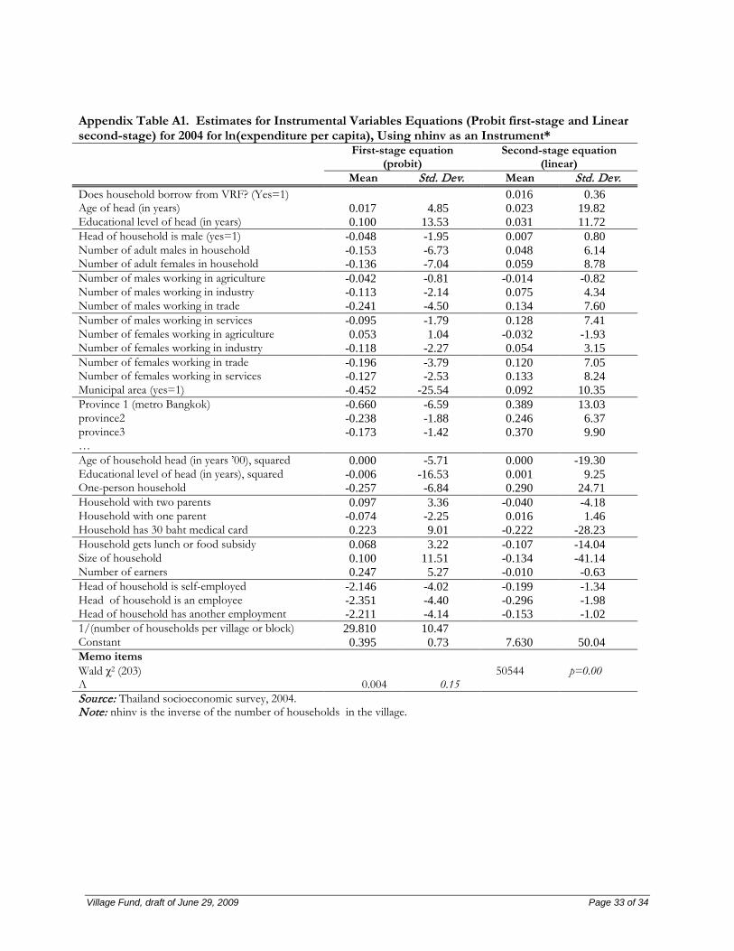
Village Fund, draft of June 29, 2009 Page 33 of 34
Appendix Table A1. Estimates for Instrumental Variables Equations (Probit first-stage and Linear second-stage) for 2004 for ln(expenditure per capita), Using nhinv as an Instrument*
First-stage equation
(probit) Second-stage equation
(linear) Mean Std. Dev. Mean Std. Dev.
Does household borrow from VRF? (Yes=1) 0.016 0.36 Age of head (in years) 0.017 4.85 0.023 19.82 Educational level of head (in years) 0.100 13.53 0.031 11.72 Head of household is male (yes=1) -0.048 -1.95 0.007 0.80 Number of adult males in household -0.153 -6.73 0.048 6.14 Number of adult females in household -0.136 -7.04 0.059 8.78 Number of males working in agriculture -0.042 -0.81 -0.014 -0.82 Number of males working in industry -0.113 -2.14 0.075 4.34 Number of males working in trade -0.241 -4.50 0.134 7.60 Number of males working in services -0.095 -1.79 0.128 7.41 Number of females working in agriculture 0.053 1.04 -0.032 -1.93 Number of females working in industry -0.118 -2.27 0.054 3.15 Number of females working in trade -0.196 -3.79 0.120 7.05 Number of females working in services -0.127 -2.53 0.133 8.24 Municipal area (yes=1) -0.452 -25.54 0.092 10.35 Province 1 (metro Bangkok) -0.660 -6.59 0.389 13.03 province2 -0.238 -1.88 0.246 6.37 province3 -0.173 -1.42 0.370 9.90 … Age of household head (in years ’00), squared 0.000 -5.71 0.000 -19.30 Educational level of head (in years), squared -0.006 -16.53 0.001 9.25 One-person household -0.257 -6.84 0.290 24.71 Household with two parents 0.097 3.36 -0.040 -4.18 Household with one parent -0.074 -2.25 0.016 1.46 Household has 30 baht medical card 0.223 9.01 -0.222 -28.23 Household gets lunch or food subsidy 0.068 3.22 -0.107 -14.04 Size of household 0.100 11.51 -0.134 -41.14 Number of earners 0.247 5.27 -0.010 -0.63 Head of household is self-employed -2.146 -4.02 -0.199 -1.34 Head of household is an employee -2.351 -4.40 -0.296 -1.98 Head of household has another employment -2.211 -4.14 -0.153 -1.02 1/(number of households per village or block) 29.810 10.47 Constant 0.395 0.73 7.630 50.04 Memo items Wald χ2 (203) 50544 p=0.00 Λ 0.004 0.15 Source: Thailand socioeconomic survey, 2004. Note: nhinv is the inverse of the number of households in the village.

Village Fund, draft of June 29, 2009 Page 34 of 34
Appendix Table A2. Estimated Equations for the Panel Instrumental Variables Analysis for ln(expenditure per capita), VRF Borrowers in 2004 vs. Non-Borrowers First-stage equation Second-stage equation
Coeffi-cient t-statistic p-value
Coeffi-cient t-statistic p-value
Did household borrow from VRF? (Yes=1) 0.179 3.19 0.001 Age of head (in years) 0.010 1.59 0.113 0.011 1.81 0.070 Educational level of head (in years) 0.048 3.53 0.000 0.002 0.20 0.840 Head of household is male (yes=1) -0.120 -3.13 0.002 0.044 1.16 0.245 Number of adult males in household 0.030 1.31 0.189 -0.065 -2.94 0.003 Number of adult females in household -0.012 -0.55 0.582 -0.161 -7.99 0.000 Number of males working in agriculture -0.135 -2.28 0.022 -0.170 -2.96 0.003 Number of males working in industry -0.068 -1.12 0.262 -0.121 -2.06 0.039 Number of males working in trade -0.094 -1.49 0.138 -0.110 -1.82 0.069 Number of males working in services -0.090 -1.54 0.124 -0.041 -0.72 0.469 Number of females working in agriculture -0.100 -1.72 0.086 -0.119 -2.11 0.035 Number of females working in industry -0.121 -2.00 0.046 -0.044 -0.75 0.455 Number of females working in trade -0.083 -1.32 0.186 -0.091 -1.51 0.131 Number of females working in services -0.039 -0.66 0.508 -0.056 -0.99 0.320 Age of household head (in years ’000), squared -0.032 -0.58 0.560 -0.107 -2.02 0.043 Educational level of head (in years ‘000), squared -0.015 -0.03 0.980 0.312 0.54 0.590 One-person household -0.042 -0.96 0.336 0.313 7.51 0.000 Household with two parents -0.012 -0.31 0.756 -0.144 -3.94 0.000 Household with one parent -0.085 -2.25 0.025 -0.014 -0.37 0.710 Household has 30 baht medical card 0.082 3.07 0.002 -0.089 -3.38 0.001 Household gets lunch or food subsidy 0.107 5.44 0.000 -0.027 -1.31 0.192 Head of household is self-employed 0.997 2.65 0.008 0.424 1.16 0.247 Head of household is an employee 0.958 2.55 0.011 0.418 1.14 0.253 Head of household has another employment 0.925 2.47 0.014 0.392 1.08 0.282 Number of earners in household 0.111 1.98 0.047 0.136 2.52 0.012 Village size × Educational level of head × 1000 -0.128 -2.96 0.003 Is there a VRF in village? (yes=1) 0.364 10.17 0.000 VRF in village × Educational level of head -0.005 -0.90 0.367 Constant -1.668 -4.23 0.000 7.312 18.88 0.000 Memo items: Hausman χ2 5.03 1.00 Number of observations 6,674 F-test of coefficients 17.93 (27,3308) 0.00 Wald χ2 test 3,007,000 (25) 0.00
F-test that ui=0 0.79 (3338,3308
) 1.00 3.10 (3338,3310)
0.00
R2: within / between / overall 0.127 0.016 0.042 0.099 0.186 0.168 Source: Thailand Socioeconomic Surveys of 2002 and 2004.
i From the panel of 5,054 households, we have the following breakdown of the number of households:
Did not borrow from VRF in 2004 Borrowed from VRF in 2004 Did not borrow from VRF in 2002 2,291 1,048 Borrowed from the VRF in 2002 303 1,412