Dual-fitting analysis of Greedy for Set Cover

We showed earlier that the greedy algorithm for set cover gives a Hn approximation

We will show that greedy produces a solution of cost at most Hn OPTLP

Note that OPTLP ≤ OPT

For this we need the dual of the LP for set cover

Primal and Dual for Set cover

Primal: mini=1m c(i) x(i)

∑i: e ∈ Six(i) ≥ 1 for each e ∈ Ux(i) ≥ 0 1 ≤ i ≤ m

Dual: max ∑e ∈ U y(e)∑e ∈ Si

y(e) ≤ c(i) for 1 ≤ i ≤ my(e) ≥ 0 e ∈ U

Dual-fitting

Recall the analysis of Hn approximation for greedy. Essentially dual-fitting in disguise as we see now.

Let hj be the index of set picked by Greedy in iteration jLet S’hj

be the new elements covered by Shj: that is those

elements covered in iteration jfor each e in S’hj

we set p(e) = c(hj)/|S’hj|

Dual-fitting

Note that by construction ∑e p(e) = cost of solution output by Greedy

Define y’(e) = p(e)/Hn

Lemma: y’ is a feasible solution to the dual LP

Assuming lemma, ∑e y’(e) ≤ OPTLP (by weak duality).Therefore cost of Greedy ≤ Hn OPTLP

Dual-fitting

Define y’(e) = p(e)/Hn

Lemma: y’ is a feasible solution to the dual LP

Need to show that for any set Si∑e in Si

y’(e) ≤ c(i) or in other words ∑e in Si

p(e) ≤ Hn c(i)

Renumber elements s.t e1, e2, ..., en are covered in that order

Dual-fitting

Renumber elements s.t e1, e2, ..., en are covered in that order

For a set Si let its elements be ei1, ei2

, ..., eitwhere |Si| = t

for l = 1 to t we claim that p(eil) ≤ c(i)/(t-l+1)

This is because when eitwas covered, Greedy could have

picked Si at density c(i)/(t-l+1)

Dual-fitting

for l = 1 to t we claim that p(eil) ≤ c(i)/(t -l+1)

This is because when eilwas covered, Greedy could have

picked Si at density c(i)/(t-l+1)

Therefore ∑e ∈ Sip(e) ≤ ∑

l=1t c(i)/(t-l+1) ≤ c(i) Ht

Remark: notice that the above analysis shows that Greedy’s cost is can be upper bounded by Hk OPTLPwhere k is the size of the largest set

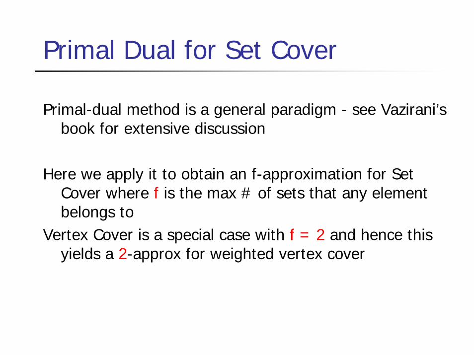
Primal Dual for Set Cover

Primal-dual method is a general paradigm - see Vazirani’s book for extensive discussion

Here we apply it to obtain an f-approximation for Set Cover where f is the max # of sets that any element belongs to

Vertex Cover is a special case with f = 2 and hence this yields a 2-approx for weighted vertex cover

Primal Dual for Set Cover

We obtain a feasible integral primal solution x and a feasible dual solution y

The pair (x,y) satisfy primal complementary slackness condition

x(i) > 0 implies ∑e ∈ Siy(e) = c(i)

since x is an integral solutionx(i) = 1 implies ∑e ∈ Si

y(e) = c(i)

Cost of solution

If we can find such a pair (x, y) then cost of solution is∑i c(i) x(i) = ∑i x(i) ∑e ∈ Si

y(e)

Changing the order of summation≤∑e y(e) ∑i: e ∈ Si

x(i)≤∑e y(e) f

Since y is feasible ∑e y(e) ≤ OPTLP

Therefore cost of solution ≤ f OPTLP ≤ f OPT

Primal-Dual algorithm

Start with feasible dual y = 0 and infeasible primal x = 0While some element is not covered

increase y(e) for all uncovered e uniformly until some constraint becomes tight (that is for some i, ∑e ∈ Si

y(e) = c(i) )

for all tight i, set x(i) = 1 and all elements in Si are covered

Primal-Dual

By induction on while loop iterations it can easily be seen that

y remains a feasible solution through out the algorithmthus at end of algorithm all elements covered are covered

(by x) and y is feasibleby construction x(i) = 1 iff i is tight hence primal

complementary slackness is satisfied for pair (x, y)

Integral Polyhedra

A rational polyhedron given by a system of inequalities Ax ≤ b is integral iff all its vertices have integer coords

Theorem: The polyhedron Ax ≤ b is integral iff for each integral w, the optimum value of max wx s.t Ax ≤ b is

an integer if it is finite.

Totally Unimodular Matrices

A 0,1 matrix A is called totally unimodular (TUM) iff for each square submatrix A’ of A, det(A’) ∈ {0,1,-1}

A simple consequence of the definition is the following

Theorem: For any integer vector b and TUM matrix A, the polyhedron A x ≤ b is an integral polyhedron

Totally Unimodular Matrices

Theorem: For any integer vector b and TUM matrix A, the polyhedron A x ≤ b is an integral polyhedron

Proof: Any vertex of the polyhedron is given by the solution to the system A’ x’ = b’ for some square non-singular sub-matrix A’ of A.

Therefore x’ = (A’)-1 b’ = ((A’)t/det(A’)) b’

Since A is TUM, det(A’) ∈ {+1, -1}. Therefore x’ is integral

since both A’ and b’ are integral

TUM matrices

Several operations preserve total unimodularityFor example we can add box constraints to Ax ≤ bThe system A x ≤ b, u ≤ x ≤ l for integer b, u, l is an

integral polyhedron if A is TUM

The dual of max c x, A ≤ b is min y b, y A = c

If c, b are integer then both primal and dual are integer polyhedra

Examples of TUM matrices

Given a directed graph G = (V, E) consider the adjacency matrix A = V x E with

A(u, e) = +1 if e = (u, v) for some v ∈ VA(u, e) = -1 if e = (v, u) for some v ∈ V

A(u, e) = 0 if u is not the head or tail of e

A is TUMFrom above one can deduce integrality of single-

commodity flows with integer capacities and also the maxflow-mincut theorem

Bipartite graphs

Bipartite graph G = (U, V, E) with U, V as the vertex sets of the two partitions

Adjacency matrix A = U x V withA(u, v) = 1 if uv ∈ E

= 0 otherwiseA is TUMFrom above one can deduce Konig’s theorem and Hall’s

theorems etc regarding matchings and vertex covers in bipartite graphs

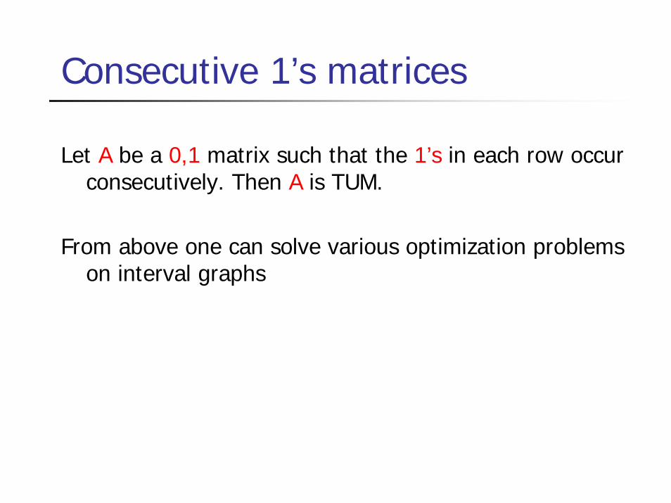
Consecutive 1’s matrices

Let A be a 0,1 matrix such that the 1’s in each row occur consecutively. Then A is TUM.

From above one can solve various optimization problems on interval graphs

Network matrices

The previous three cases are examples of network matrices. A network matrix is obtained from a directed graph G=(V, E) and a directed tree T = (V, E’) on the same vertex set. Note that the arcs of T can be oriented in any way. Given G, T we obtain a matrix A = E x E’ as follows

For e = (u,v) in E let Puv be the unique path from u to v in T (the path is simply a list of edges in E’)

A(e, e’) = +1 if e’ occurs in the direction of traversal of Puvfrom u to v

A(e, e’) = -1 if e’ occurs in the opposite direction of traversal from u to v

A(e, e’) = 0 if e’ is not in Puv

Network matrices

Theorem: Network matrices are TUM

Not all TUM matrices are network matrices

Exercise: show how each of the three classes seen before are examples of network matrices

(difficult theorem of Seymour)Theorem: Given a matrix A, poly-time algorithm to check if

A is TUM

Integer decomposability of TUM matrices

Useful to know following.

Theorem: Let x be a feasible point in A x ≤ b for some TUM A and integral b. Let k x be integral for some integer k. Then k x = x1 + x2 + ... + xk for integral vectors x1, ..., xk each of which is a feasible point in A x ≤ b.

Above also holds for system A x≤ b, l ≤ x ≤ u for integralbounds l, u