Embed Size (px)
Citation preview
DZD DPZ 10 – Image spectroscopy
Doc. Dr. Ing. Jiří Horák - Ing. Tomáš Peňáz, Ph.D.
Institut geoinformatiky
VŠB-TU Ostrava
Basic info
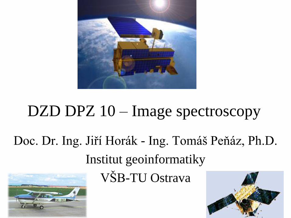
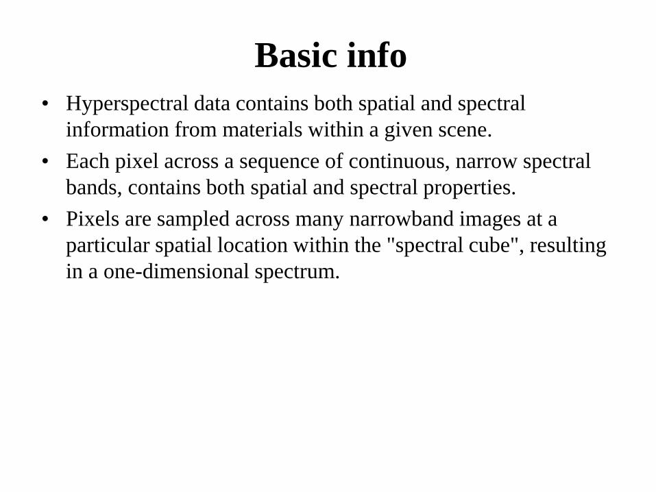
• Hyperspectral data contains both spatial and spectral
information from materials within a given scene.
• Each pixel across a sequence of continuous, narrow spectral
bands, contains both spatial and spectral properties.
• Pixels are sampled across many narrowband images at a
particular spatial location within the "spectral cube", resulting
in a one-dimensional spectrum.
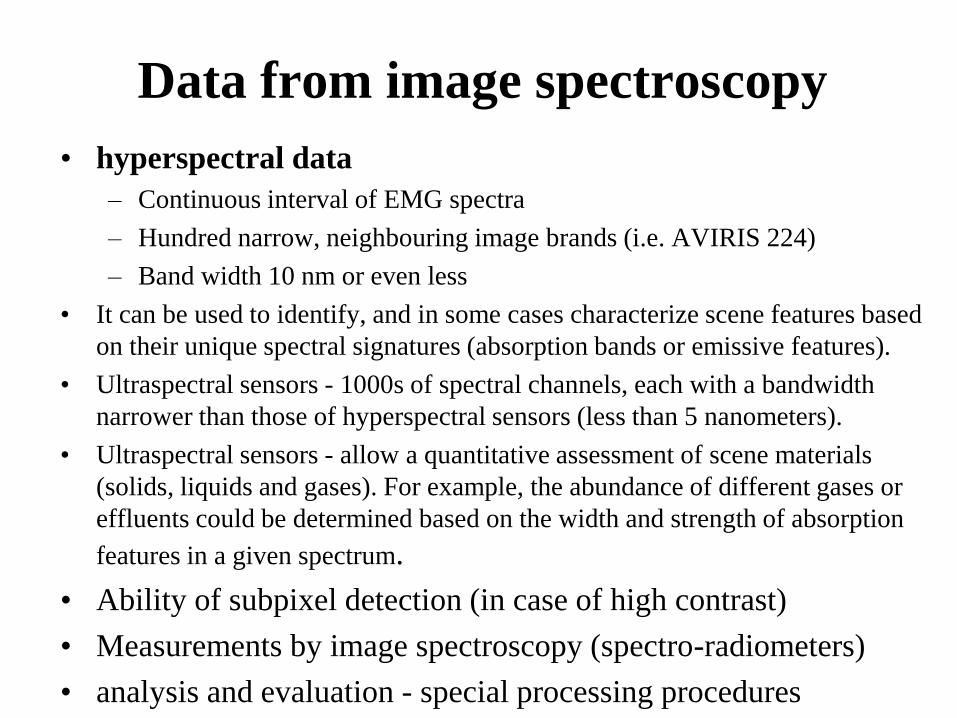
Data from image spectroscopy
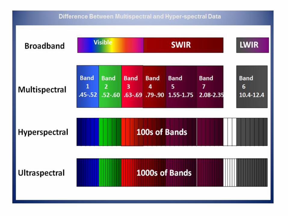
• hyperspectral data
– Continuous interval of EMG spectra
– Hundred narrow, neighbouring image brands (i.e. AVIRIS 224)
– Band width 10 nm or even less
• It can be used to identify, and in some cases characterize scene features based
on their unique spectral signatures (absorption bands or emissive features).
• Ultraspectral sensors - 1000s of spectral channels, each with a bandwidth
narrower than those of hyperspectral sensors (less than 5 nanometers).
• Ultraspectral sensors - allow a quantitative assessment of scene materials
(solids, liquids and gases). For example, the abundance of different gases or
effluents could be determined based on the width and strength of absorption
features in a given spectrum.
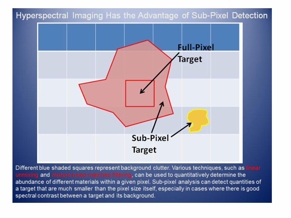
• Ability of subpixel detection (in case of high contrast)
• Measurements by image spectroscopy (spectro-radiometers)
• analysis and evaluation - special processing procedures
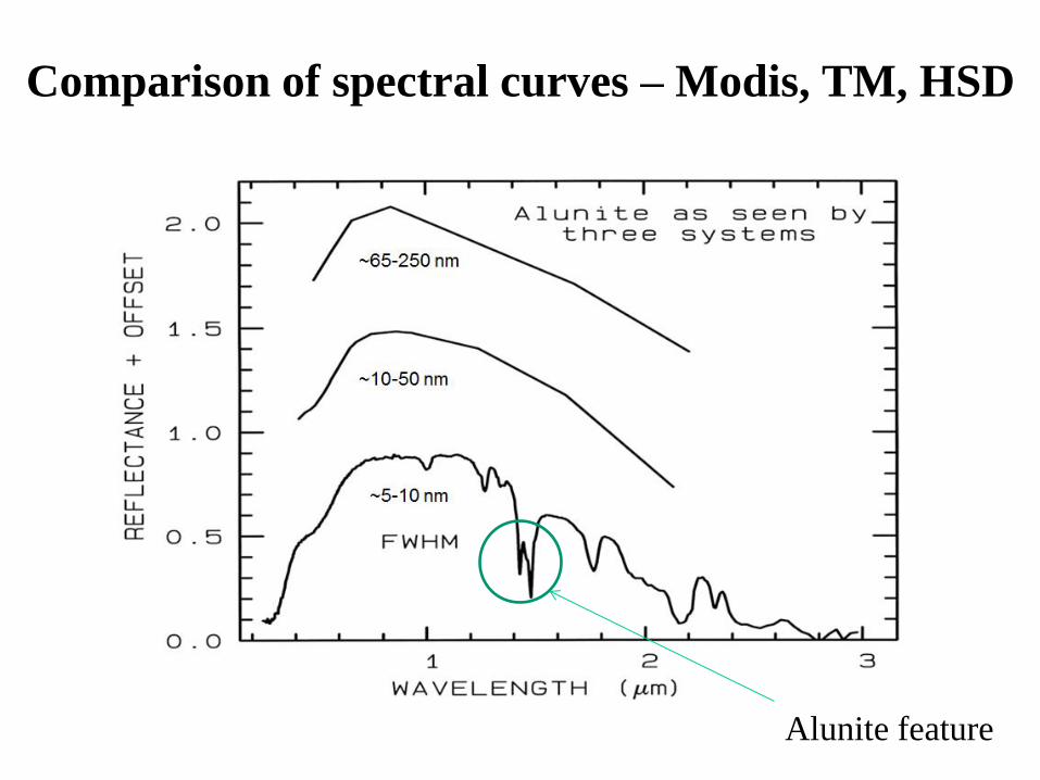
Comparison of spectral curves – Modis, TM, HSD
Alunite feature
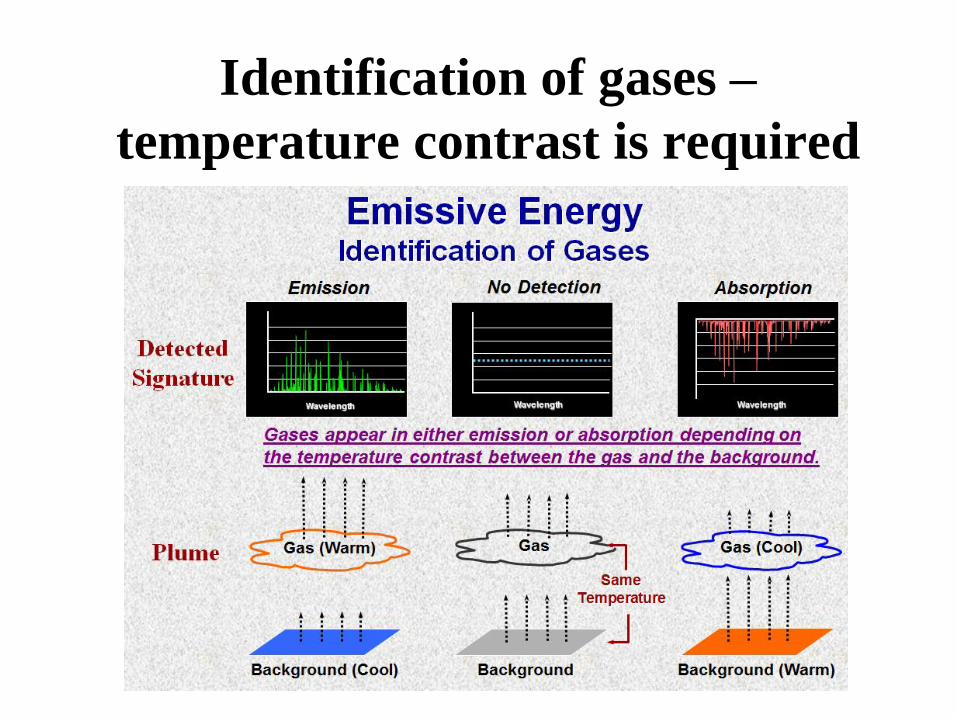
Identification of gases –
temperature contrast is required
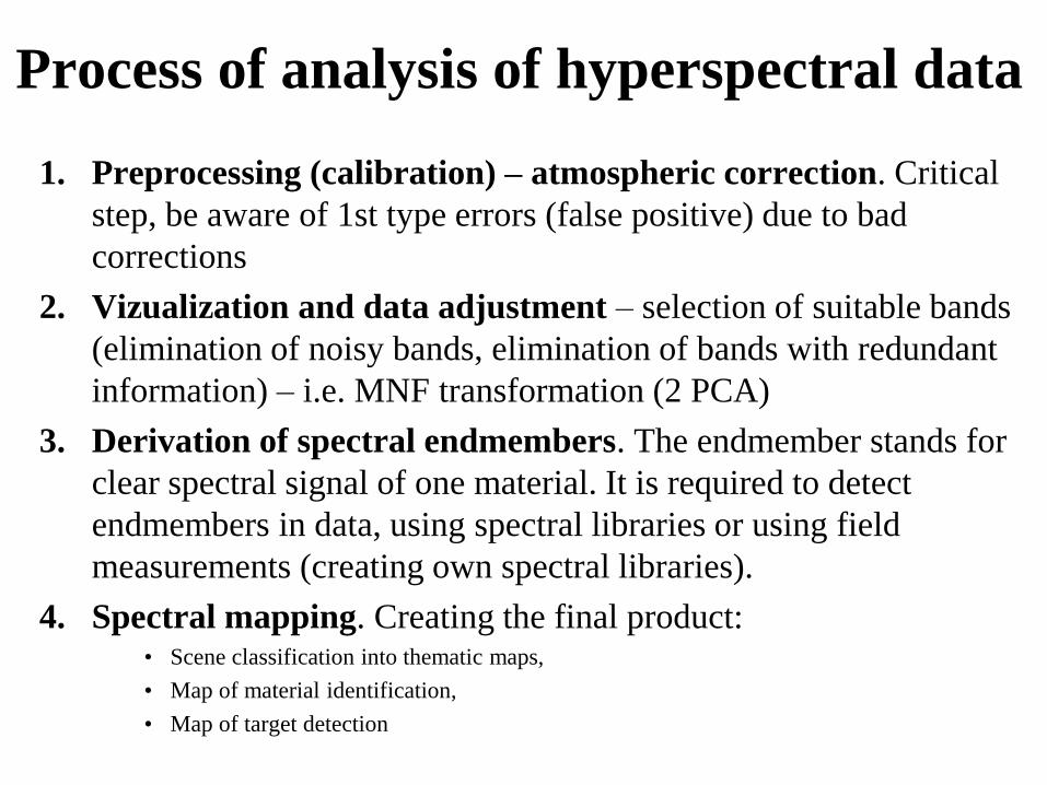
Process of analysis of hyperspectral data
1. Preprocessing (calibration) – atmospheric correction. Critical
step, be aware of 1st type errors (false positive) due to bad
corrections
2. Vizualization and data adjustment – selection of suitable bands
(elimination of noisy bands, elimination of bands with redundant
information) – i.e. MNF transformation (2 PCA)
3. Derivation of spectral endmembers. The endmember stands for
clear spectral signal of one material. It is required to detect
endmembers in data, using spectral libraries or using field
measurements (creating own spectral libraries).
4. Spectral mapping. Creating the final product: • Scene classification into thematic maps,
• Map of material identification,
• Map of target detection
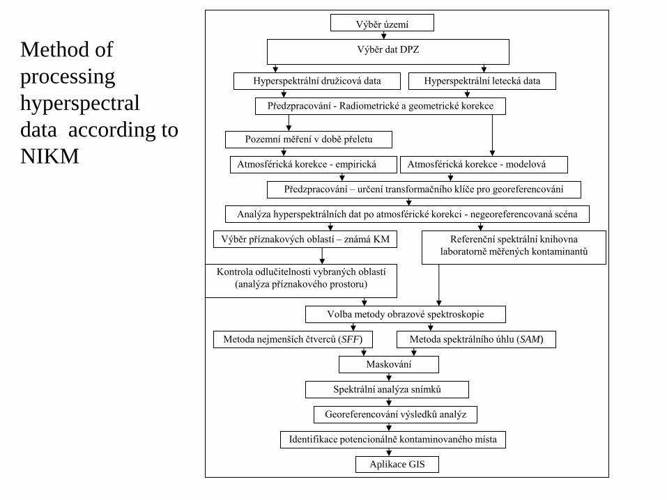
Method of
processing
hyperspectral
data according to
NIKM
Výběr území
Hyperspektrální družicová data Hyperspektrální letecká data
Pozemní měření v době přeletu
Atmosférická korekce - empirická
Předzpracování – určení transformačního klíče pro georeferencování
Předzpracování - Radiometrické a geometrické korekce
Atmosférická korekce - modelová
Výběr příznakových oblastí – známá KM
Kontrola odlučitelnosti vybraných oblastí
(analýza příznakového prostoru)
Výběr dat DPZ
Analýza hyperspektrálních dat po atmosférické korekci - negeoreferencovaná scéna
Spektrální analýza snímků
Identifikace potencionálně kontaminovaného místa
Aplikace GIS
Referenční spektrální knihovna
laboratorně měřených kontaminantů
Georeferencování výsledků analýz
Volba metody obrazové spektroskopie
Metoda nejmenších čtverců (SFF) Metoda spektrálního úhlu (SAM)
Maskování
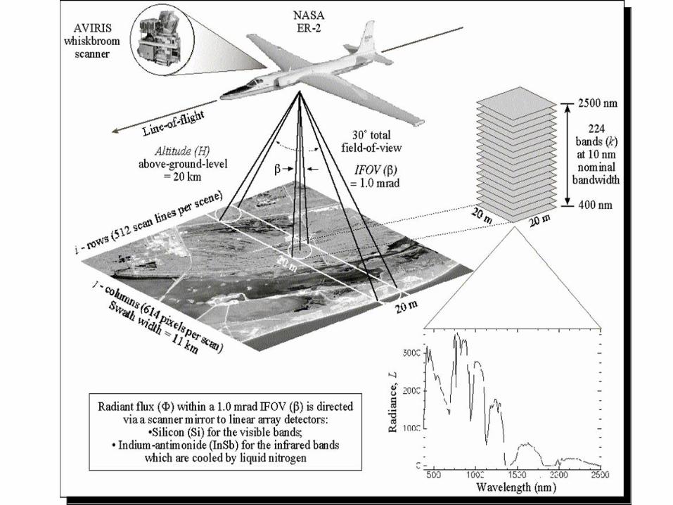
Collection of hyperspectral data
• Satellite (EO-1 Hyperion)
• Airborne (AVIRIS)
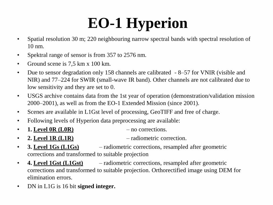
EO-1 Hyperion • Spatial resolution 30 m; 220 neighbouring narrow spectral bands with spectral resolution of
10 nm.
• Spektral range of sensor is from 357 to 2576 nm.
• Ground scene is 7,5 km x 100 km.
• Due to sensor degradation only 158 channels are calibrated - 8–57 for VNIR (visible and
NIR) and 77–224 for SWIR (small-wave IR band). Other channels are not calibrated due to
low sensitivity and they are set to 0.
• USGS archive contains data from the 1st year of operation (demonstration/validation mission
2000–2001), as well as from the EO-1 Extended Mission (since 2001).
• Scenes are available in L1Gst level of processing, GeoTIFF and free of charge.
• Following levels of Hyperion data preprocessing are available:
• 1. Level 0R (L0R) – no corrections.
• 2. Level 1R (L1R) – radiometric correction.
• 3. Level 1Gs (L1Gs) – radiometric corrections, resampled after geometric
corrections and transformed to suitable projection
• 4. Level 1Gst (L1Gst) – radiometric corrections, resampled after geometric
corrections and transformed to suitable projection. Orthorectified image using DEM for
elimination errors.
• DN in L1G is 16 bit signed integer.
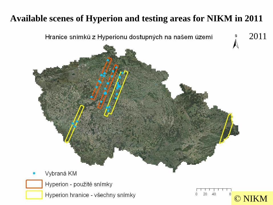
Available scenes of Hyperion and testing areas for NIKM in 2011
2011
© NIKM
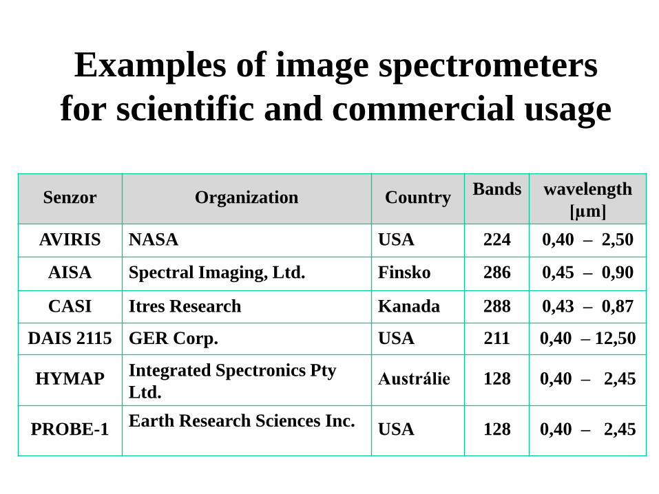
Examples of image spectrometers
for scientific and commercial usage
Senzor Organization Country Bands wavelength
[µm]
AVIRIS NASA USA 224 0,40 – 2,50
AISA Spectral Imaging, Ltd. Finsko 286 0,45 – 0,90
CASI Itres Research Kanada 288 0,43 – 0,87
DAIS 2115 GER Corp. USA 211 0,40 – 12,50
HYMAP Integrated Spectronics Pty
Ltd. Austrálie 128 0,40 – 2,45
PROBE-1 Earth Research Sciences Inc.
USA 128 0,40 – 2,45
Collection of hyperspectral data
• AVIRIS airborne hyperspectral imaging sensor obtains
spectral data over 224 continuous channels, each with a
bandwidth of 10 nm over a spectral range from 400 to 2500
nanometers.
• An example of an operational space-based hyperspectral
imaging platform, is the Air Force Research Lab's TacSat-
3/ARTEMIS sensor, which has 400 continuous spectral
channels, each with a bandwidth of 5 nm.
Mechanooptický spektrometr
Vizualization of hyperspectral data
• Curvatures of spectral behaviour
• Graphical representation in spectral space
• Image cube
Curvatures of spectral behaviour
• Absorption bands
• Typical shape of curvatures for some materials
– identification
– discrimination
• Libraries of curvatures of spectral behaviour:
– SW - ERDAS Imagine, ENVI, TNTmips, ER-Mapper
– www:
• http://speclib.jpl.nasa.gov/
• http://speclab.cr.usgs.gov/spectral.lib04/spectral-lib04.html
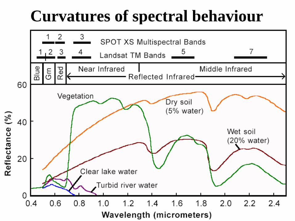
Curvatures of spectral behaviour
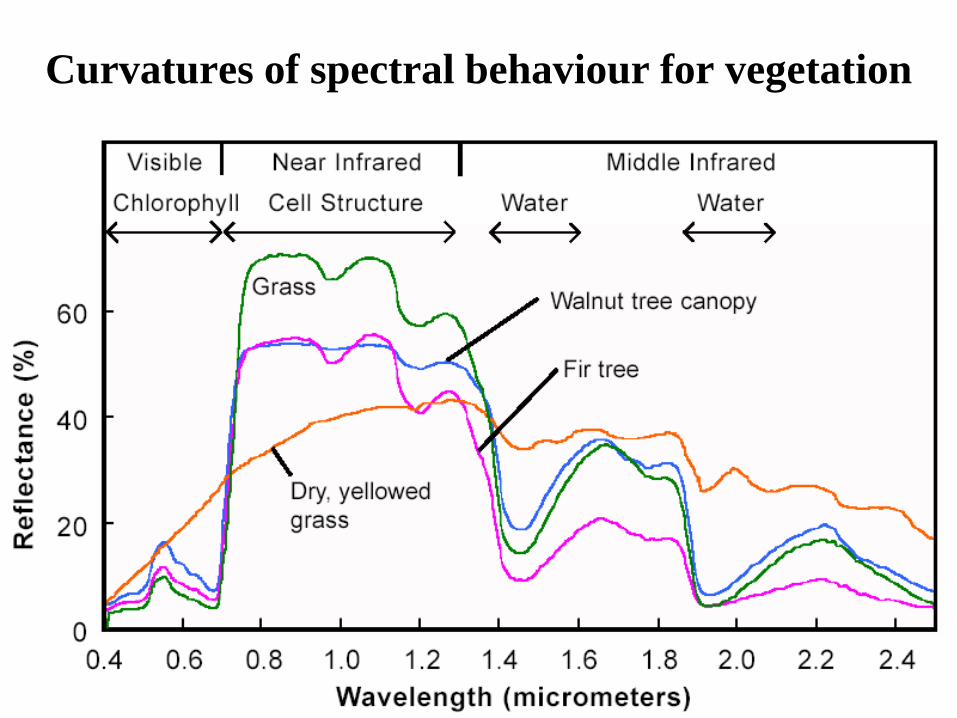
Curvatures of spectral behaviour for vegetation
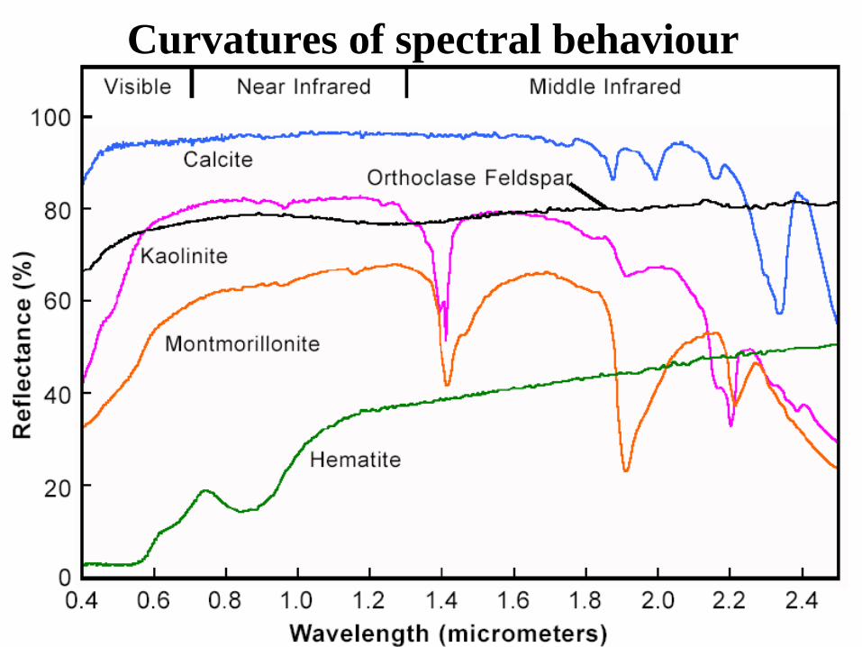
Curvatures of spectral behaviour
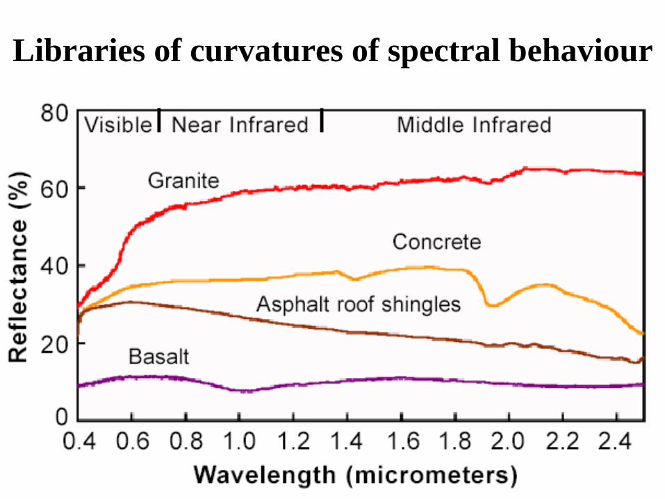
Libraries of curvatures of spectral behaviour
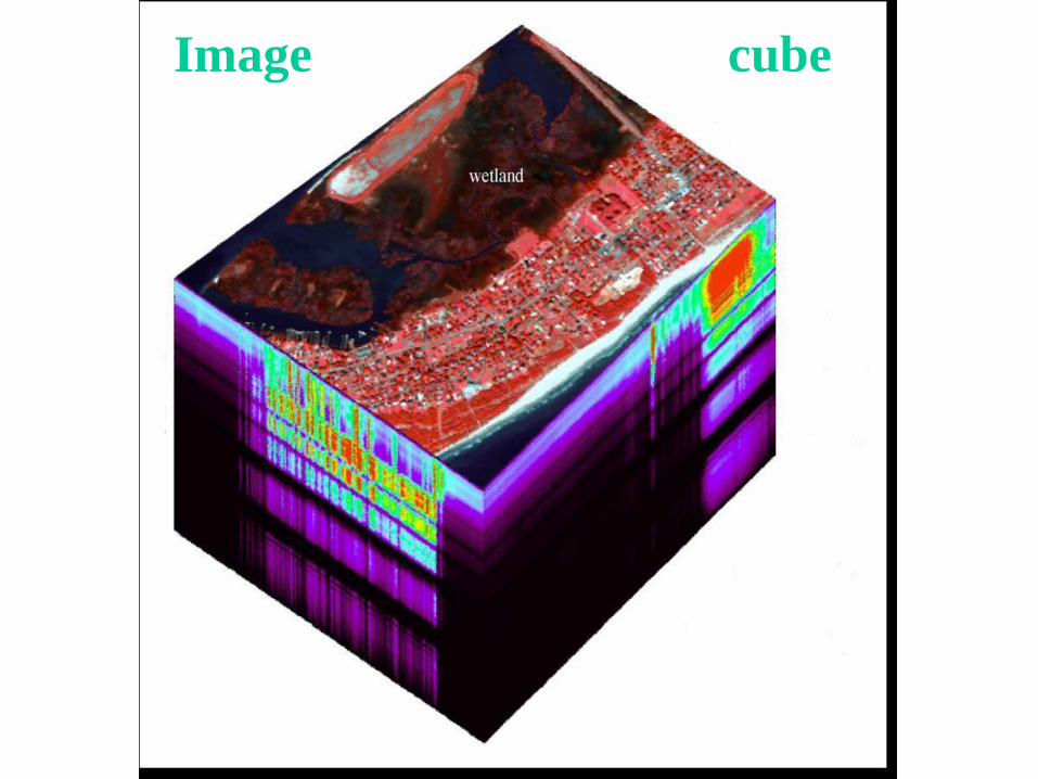
Image cube
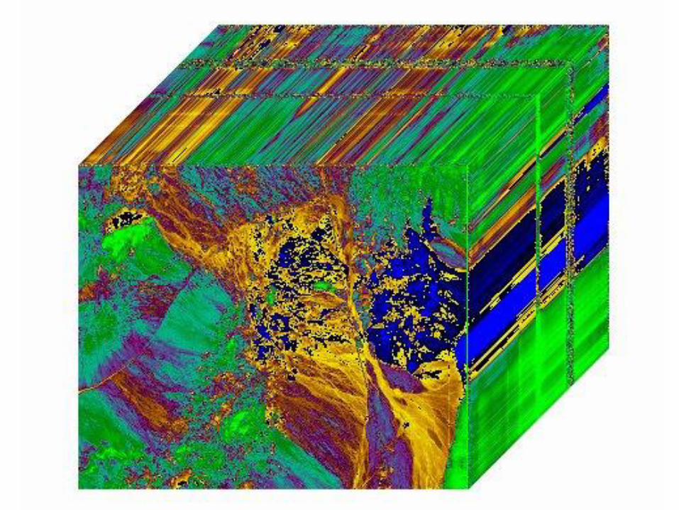
Obrazová kostka
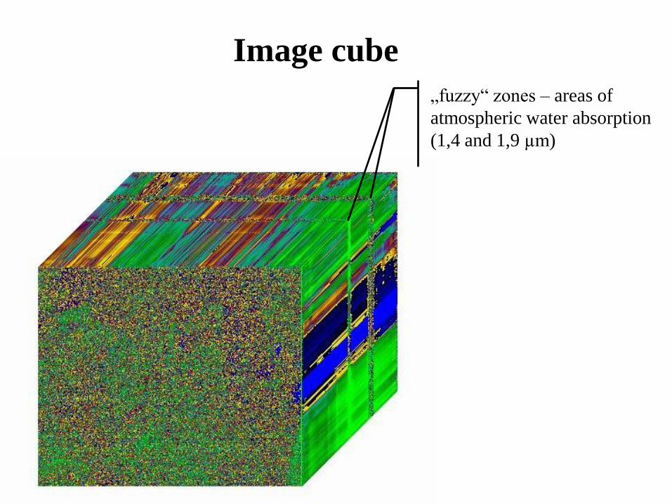
Image cube
„fuzzy“ zones – areas of
atmospheric water absorption
(1,4 and 1,9 µm)
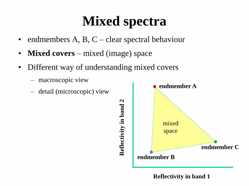
Mixed spectra
• endmembers A, B, C – clear spectral behaviour
• Mixed covers – mixed (image) space
• Different way of understanding mixed covers
– macroscopic view
– detail (microscopic) view
Reflectivity in band 1
Ref
lecti
vit
y i
n b
an
d 2
endmember A
endmember C
endmember B
mixed
space

Mixed spectra microscopic view
• Background – photon interacts with several types
of material (in the mixture)
• Mixed spectrum – nonlinear combination (difficult
description of individual shares)
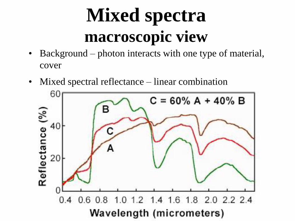
Mixed spectra macroscopic view
• Background – photon interacts with one type of material,
cover
• Mixed spectral reflectance – linear combination
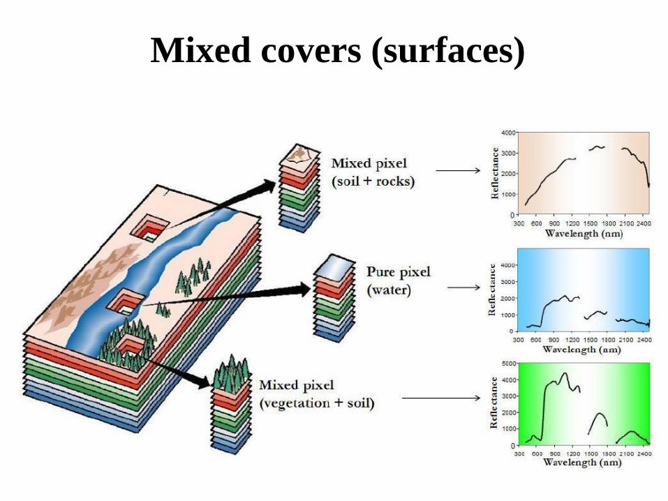
Mixed covers (surfaces)
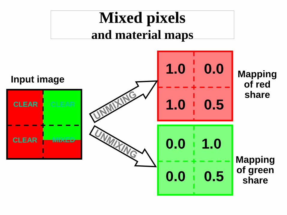
Mixed pixels and material maps
Input image 1.0
1.0
0.0
0.5
1.0 0.0
0.0 0.5
Mapping of red share
Mapping of green
share
CLEAR CLEAR
CLEAR MIXED
Preprocessing of hyperspectral data
Preprocessing of hyperspectral data
• Requirements of analysis of hyperspectral data
– atmospheric corrections
– corrections of local conditions (influences of terrain
complexity)
– Noise data elimination
Preprocessing of hyperspectral data
• methods of reflectivity conversion for hyperspectral
data
– flat field conversion
– conversion of average relative reflectance
– method of empirical line
– modelled methods
• Noise elimination in data
– Principal component analysis (PCA)
– Transformation of minimal noise fraction (MNF)
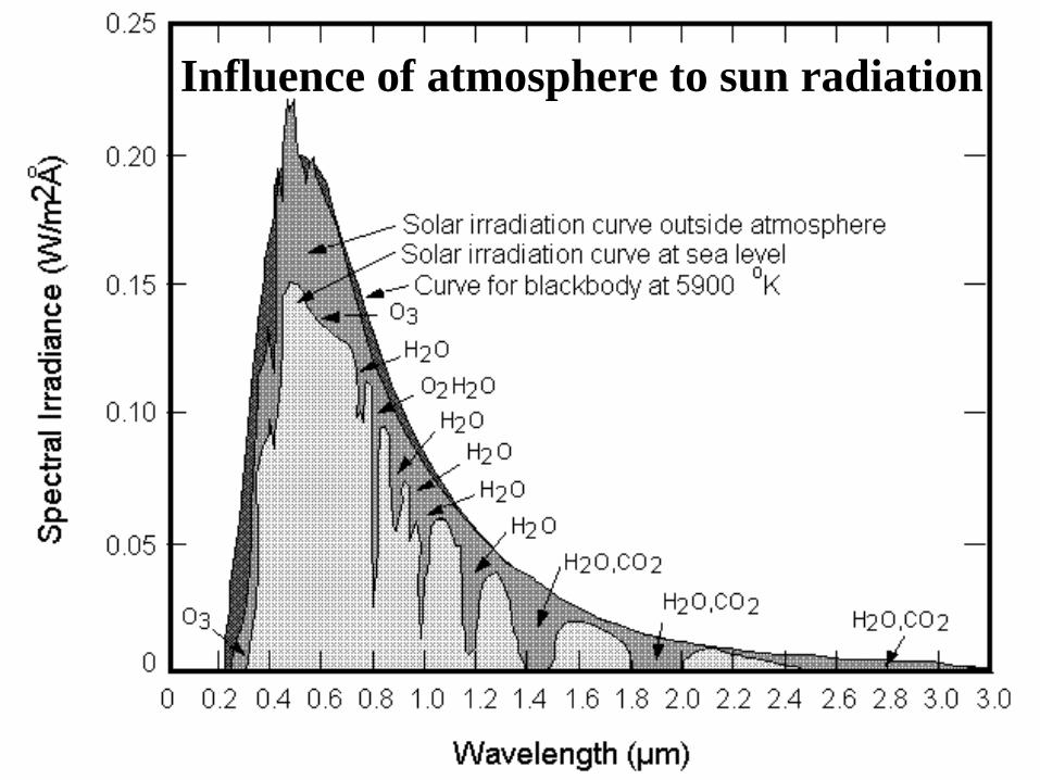
Influence of atmosphere to sun radiation
Flat Field Conversion
• Flat Field Conversion
• Average spectral response of the field is influenced by
– Solar irradiance
– atmospheric variance and absorption
• Image record from homogeneous area – so called „Flat Field“ – flat spectral curvature resp. its part
• Normalization of the image of spectral characteristics of the scene
• Conversion of the scene into „relative“ reflectance divided by average reflectance of „flat field“
Flat Field Conversion
• Selection of light areas
• Method suitable for homogeneous fields
– deserts
– dry basin of salt lake
– Light anthropogenous materials (concrete – in towns)
• method unsuitable for land with significant changes of the altitude (majority of the scene)
– Topographic Shading
– Atmospheric Path Differences
Average Relative Reflectance Conversion
• Normalization of spectral characteristics using
dividing by average value for the whole hyperspectral
record
• Such preprocessing will remove:
– topographical shadows
– changes of brightness intensity
Average Relative Reflectance Conversion
• Assumption – enough heterogeneity of records:
– eliminate spatial variability represented by spectral characteristics
– calculate average value of spectral characteristics (similar to flat field conversion)
• Suitable only for some regions
• May create spurious spectral characteristics
Other methods of spectral reflectance conversion
• Focused on mineral mapping
• Influence of atmosphere to the change of spectral reflectance:
– small - infrared <2; 2,5>μm
– neglectable – visible and near infrared <0,4;2,0>μm
• In case of dark materials and deep topographical shadows use approximate following correction of bands:
– Adjust minimal brightness value or average value in the shadow
– Subtract from each DN value
Empirical Line Method • Used for conversion of image data (DN) into ground
reflectance
• Measurements of ground spectral reflectance in two or more areas:
– Satisfactory enough, means distinguishable in the image
– Show substantially different DN values
• Relationship between spectral reflectance on the ground and above the atmosphere
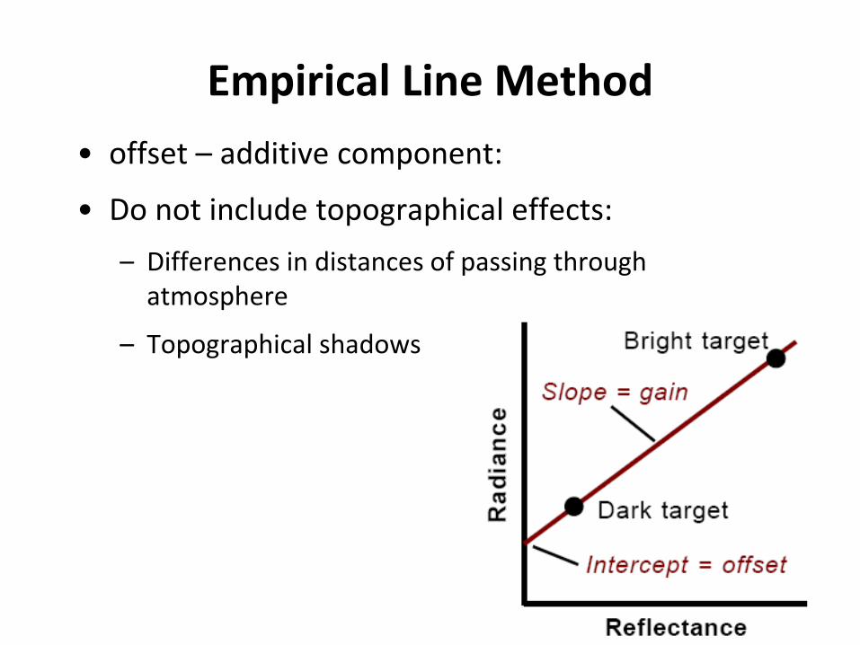
Empirical Line Method
• offset – additive component:
• Do not include topographical effects:
– Differences in distances of passing through atmosphere
– Topographical shadows
Modelling methods • Radiance conversion – simulation of sun radiance spectrum
according to the sun elevation
• Input atmospheric conditions:
– known – from field measurements
– Unknown – from estimation (using distribution of CO2, O2)
• Mixture of CO2, O2
• Scattering effect of water vapour – estimation and correction – and water absorption
• Topographical shadows may be included
• Example - model ATREM 3.0
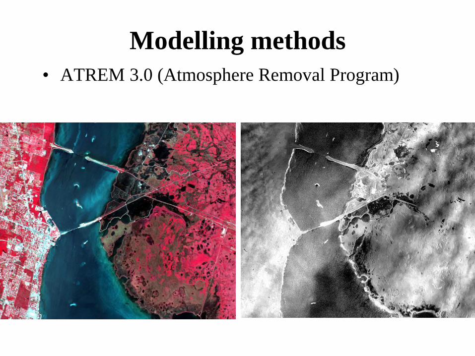
Modelling methods
• ATREM 3.0 (Atmosphere Removal Program)
Data modification (enhancement) – data
preparation before classification
PCA
• Elimination of data redundancy - numerical and
visual similarity of neighbour bands
• Information concentration in low level synthetic
bands
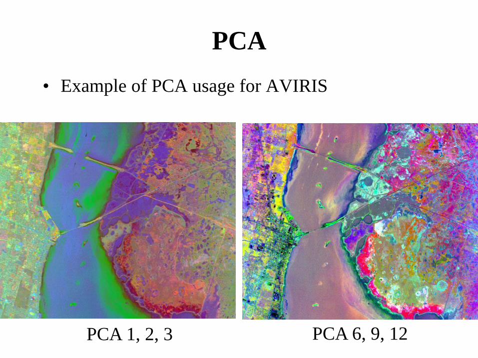
PCA
• Example of PCA usage for AVIRIS
PCA 1, 2, 3 PCA 6, 9, 12
Cross-correlation method
• Comparison of investigated band values with values of other
bands
• Calculate correlation coefficients for same pixels
• The output is a correlation raster of DN <0; 1>
• Processing by thresholding:
0 – no matching
1 – perfect match, pixel represents an elementary cover
• Robust method to brightness heterogeneity in records
Minimal Noise Fraction Transformation
(MNF) • Preliminary noise calculation in each band using spatial deviation
in brightness values
• 2 PCA follows
• Output – synthetic bands with equally distributed noise
• Bands with lower indexes contains:
– dominance of image information
– Small (neglectable) amount of noise
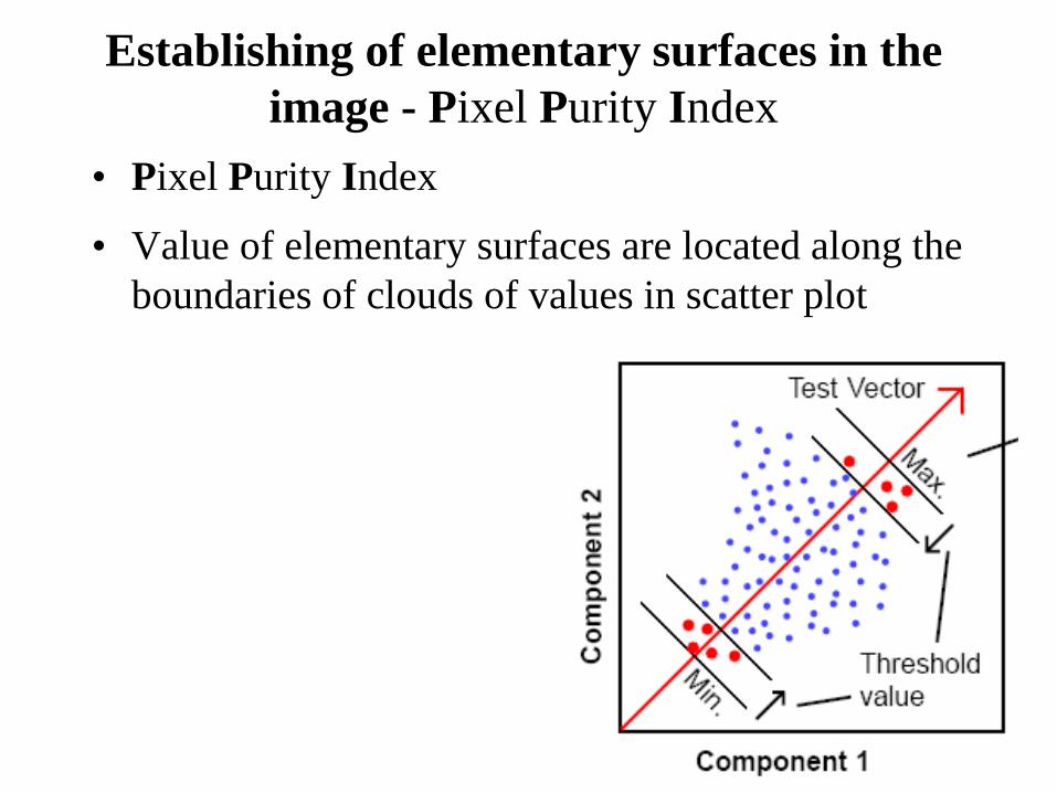
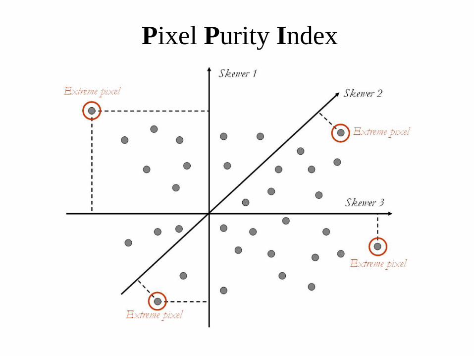
Establishing of elementary surfaces in the
image - Pixel Purity Index
• Pixel Purity Index
• Value of elementary surfaces are located along the
boundaries of clouds of values in scatter plot
Establishing of elementary surfaces in the image
• Input for PPI calculation if the result of MNF -
synthetic bands of low level – perform the linear
unmixing
• PPI is available in:
– TNTMips
– ENVI
• PPI raster as a mask for n-dimensional visual tools:
– TNTMips (n-Dimensional Visualizer )
– ENVI (n-D Visualizer )
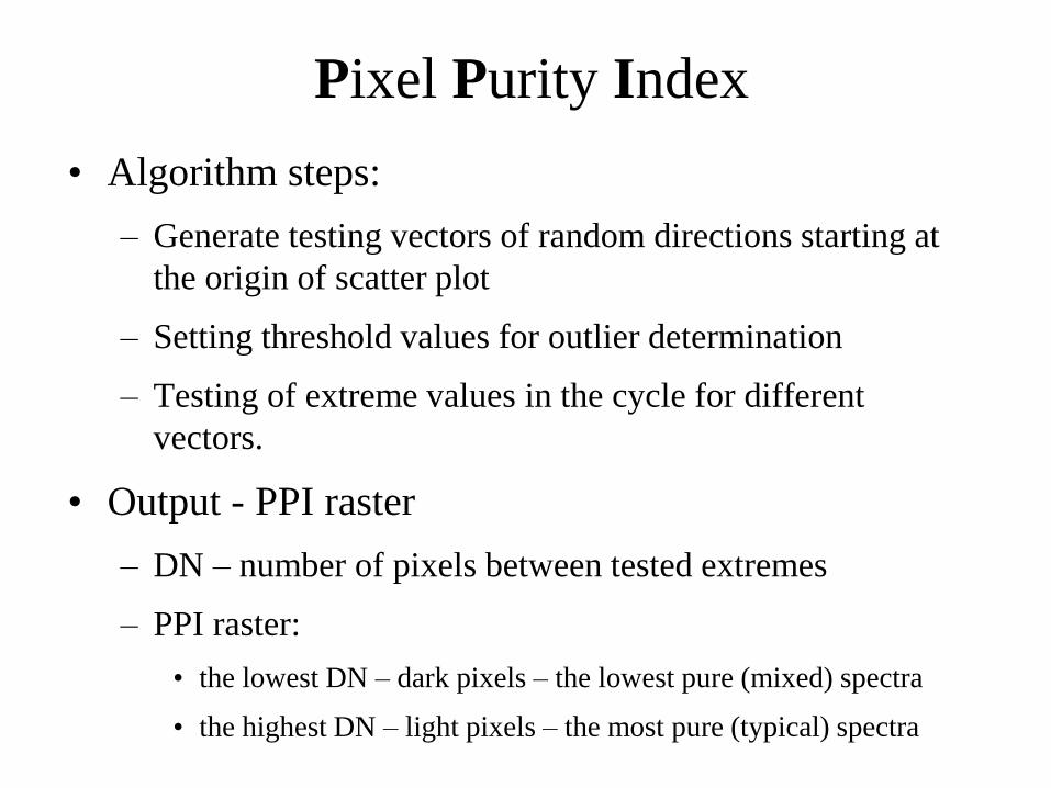
Pixel Purity Index
• Algorithm steps:
– Generate testing vectors of random directions starting at
the origin of scatter plot
– Setting threshold values for outlier determination
– Testing of extreme values in the cycle for different
vectors.
• Output - PPI raster
– DN – number of pixels between tested extremes
– PPI raster:
• the lowest DN – dark pixels – the lowest pure (mixed) spectra
• the highest DN – light pixels – the most pure (typical) spectra
Pixel Purity Index
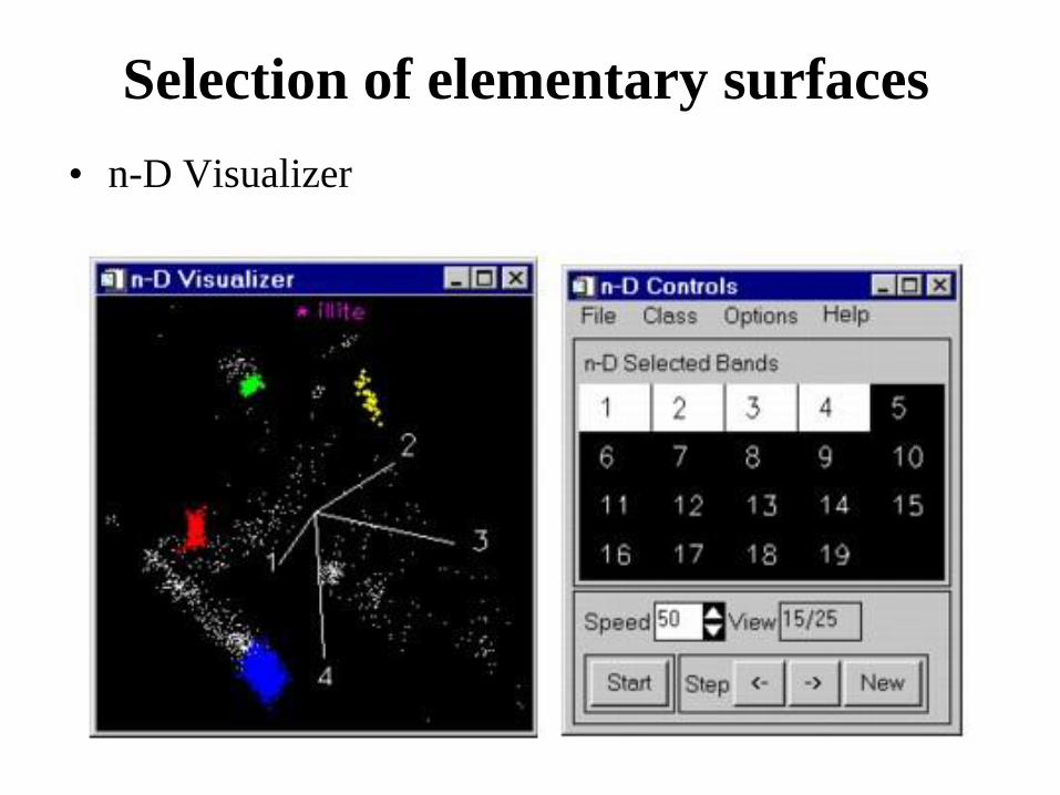
Selection of elementary surfaces
• n-D Visualizer
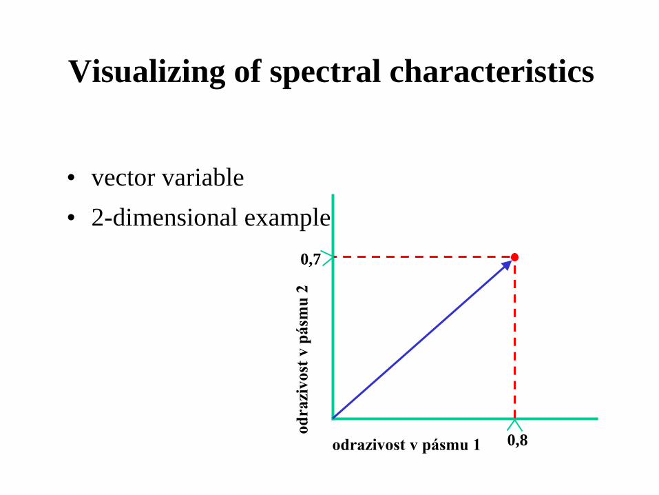
Visualizing of spectral characteristics
• vector variable
• 2-dimensional example
0,8
0,7
odrazivost v pásmu 1
od
razi
vo
st v
pásm
u 2
Classification Methods of hyperspectral data
• Classification by spectral angle (SAM)
• matched filters MF)
• Spectral Template Matching
• Spectral Feature Fitting (SSF)
• Adaptive Coherence Estimator (ACE)
• Mixture Tuned Matched Filter (MTMF)
• linear unmixing (LU)
• CEM
• MTMF/SAM
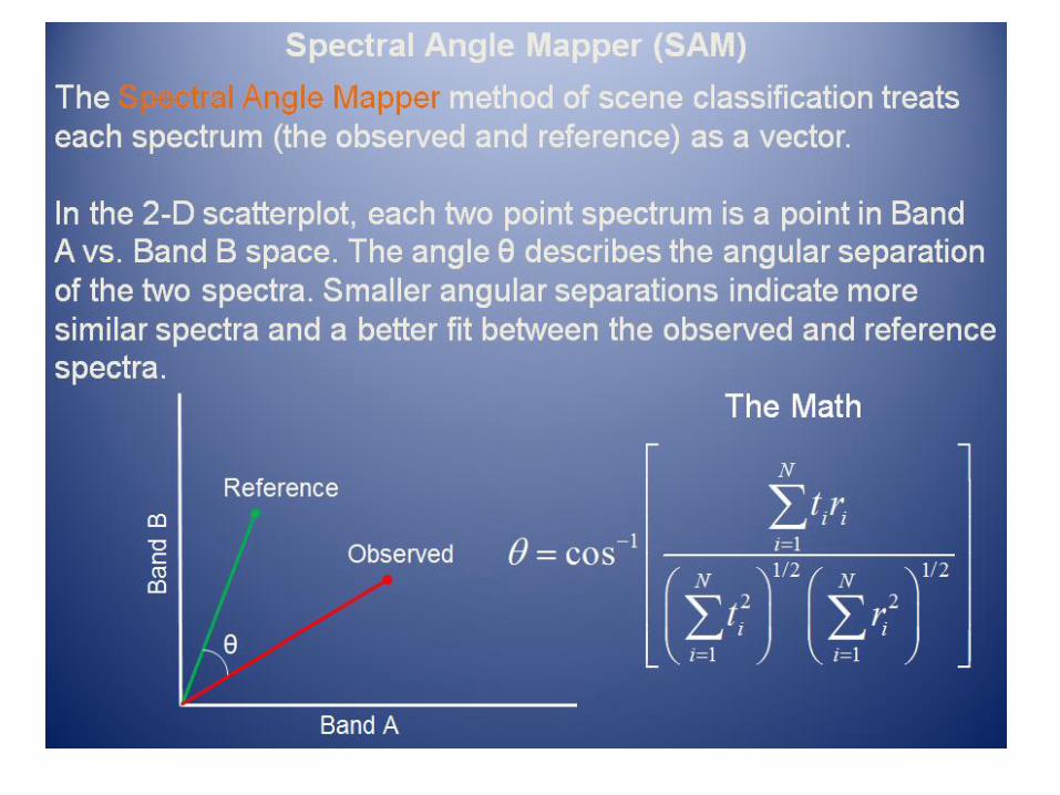
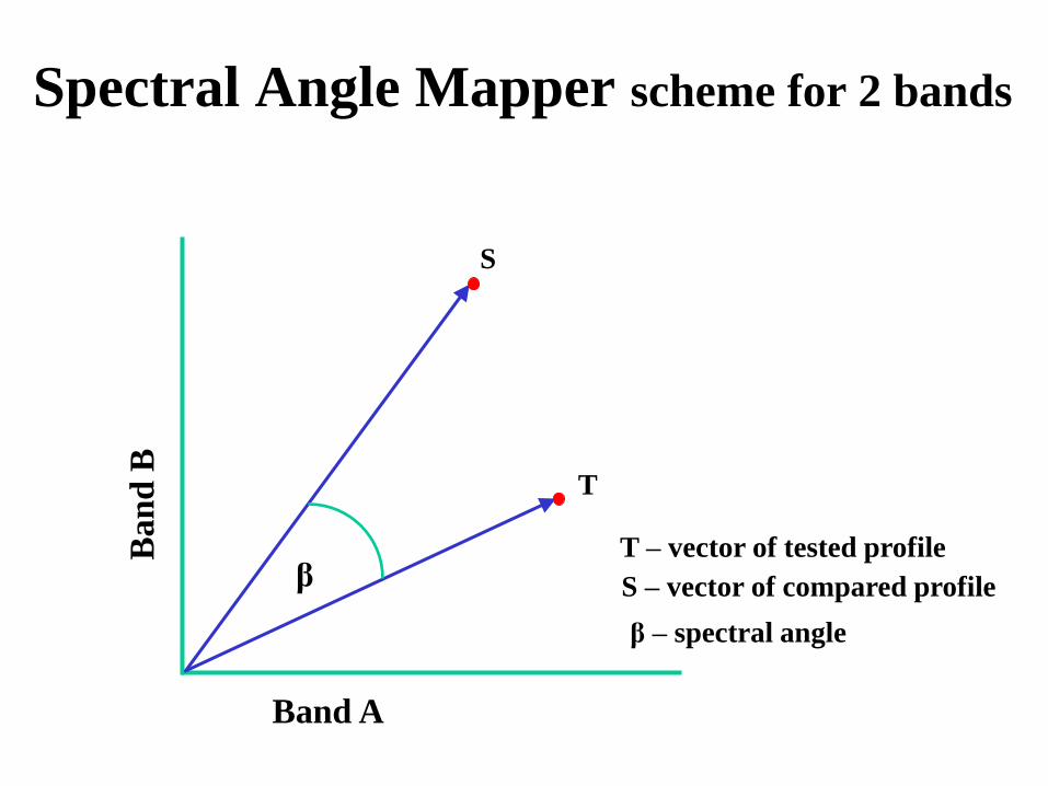
Spectral Angle Mapper scheme for 2 bands
Band A
Ban
d B
β T – vector of tested profile S – vector of compared profile
S
T
β – spectral angle
Classification by spectral angle
• Output is the raster where DN represents β
• Values of reflectance should be used but using radiation values will not cause serious errors
• The method is relatively insensitive for illumination and albedo effects
• The method do not require illumination corrections:
– Require the vector orientation (direction)
– Do not require a length of the vector
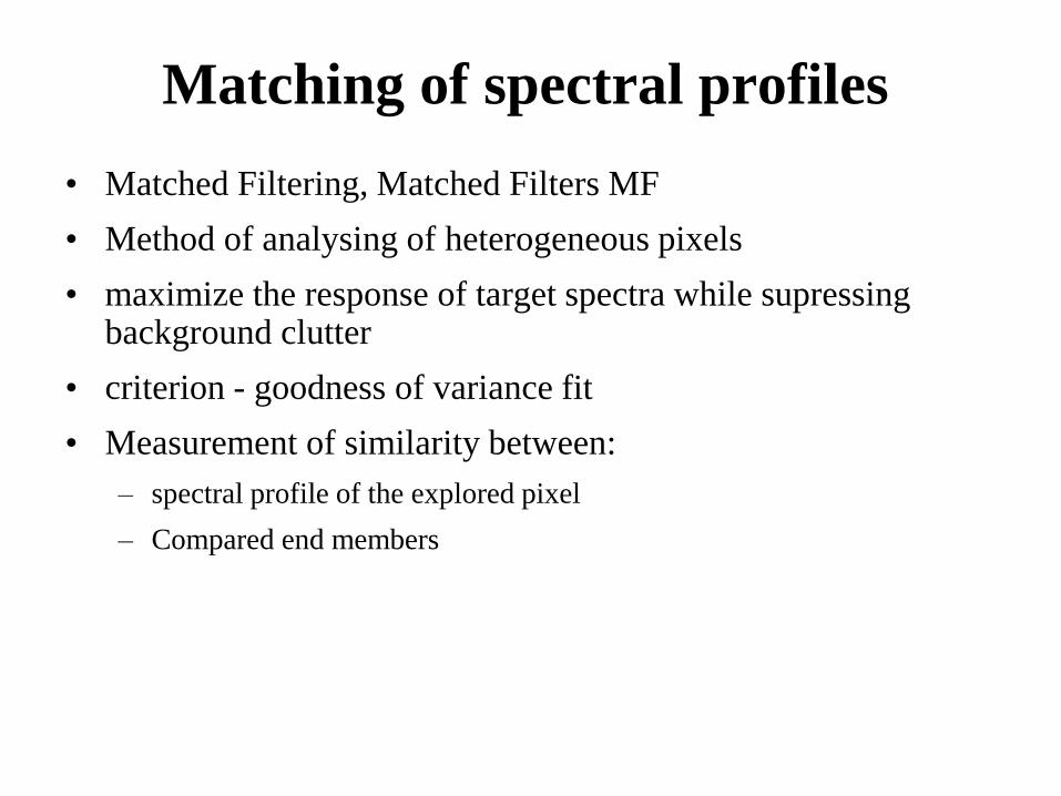
Matching of spectral profiles
• Matched Filtering, Matched Filters MF
• Method of analysing of heterogeneous pixels
• maximize the response of target spectra while supressing background clutter
• criterion - goodness of variance fit
• Measurement of similarity between:
– spectral profile of the explored pixel
– Compared end members
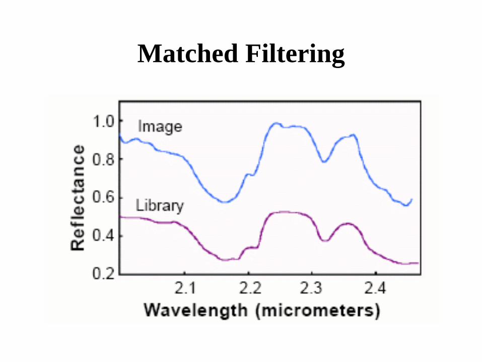
Matched Filtering
Matched Filtering
• The partial result is raster (for each compared spectral
profile - end member)
• Date type in this raster – floating point
DN = 1 => perfect match
DN < 1 => partial match
• The final result is the map of material (raster)
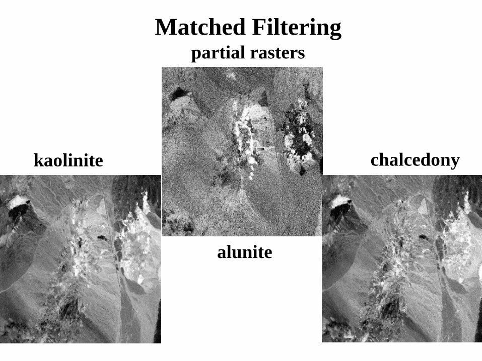
Matched Filtering partial rasters
alunite
kaolinite chalcedony
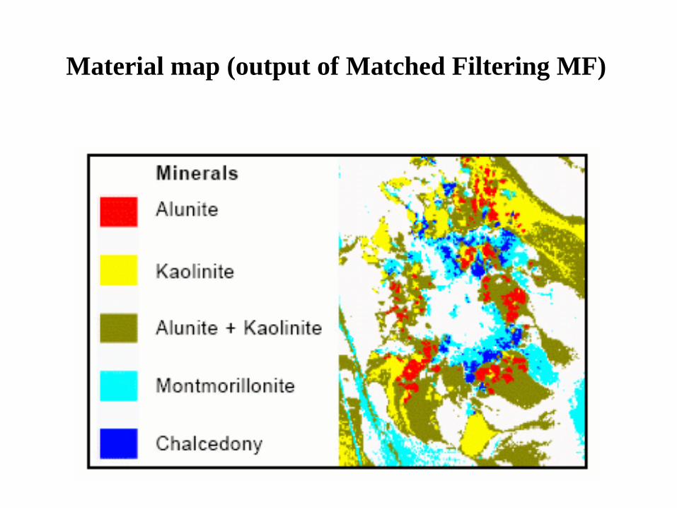
Material map (output of Matched Filtering MF)
Using spectral information for data analysis
• Limited usage of supervised classification
• Set of other methods
• DN of final raster – represents the measurement
of similarity between analysed and compared
spectra
• The risk of material exchange by those with
similar spectral behaviour
Spectral Feature Fitting (SFF)
• These methods require to transform data into reflectance and then to normalise
spectral behaviour (elimination of continuum). The continuum represents the
spectrum of surroundings which should not be taken into account for specific
absorption properties of interested material.
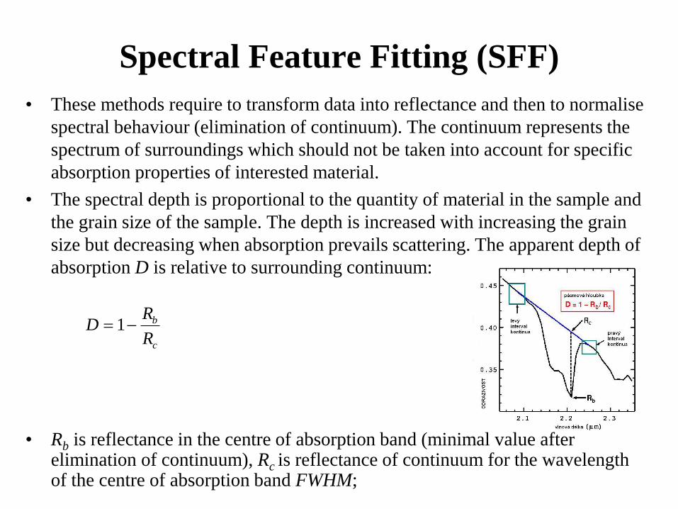
• The spectral depth is proportional to the quantity of material in the sample and
the grain size of the sample. The depth is increased with increasing the grain
size but decreasing when absorption prevails scattering. The apparent depth of
absorption D is relative to surrounding continuum:
• Rb is reflectance in the centre of absorption band (minimal value after elimination of continuum), Rc is reflectance of continuum for the wavelength of the centre of absorption band FWHM;
c
b
R
RD 1
Spectral Feature Fitting (SFF)
• Spectral behaviour (manifestation) of explored material measured by remote
sensing are not such good as manifestation of pure reference material.
• Illumination, terrain slope and atmospheric influences
• Unable direct comparison of referenced material spectra and explored material.
• Real material are almost always mixed – comparison after separation of
explored spectrum.
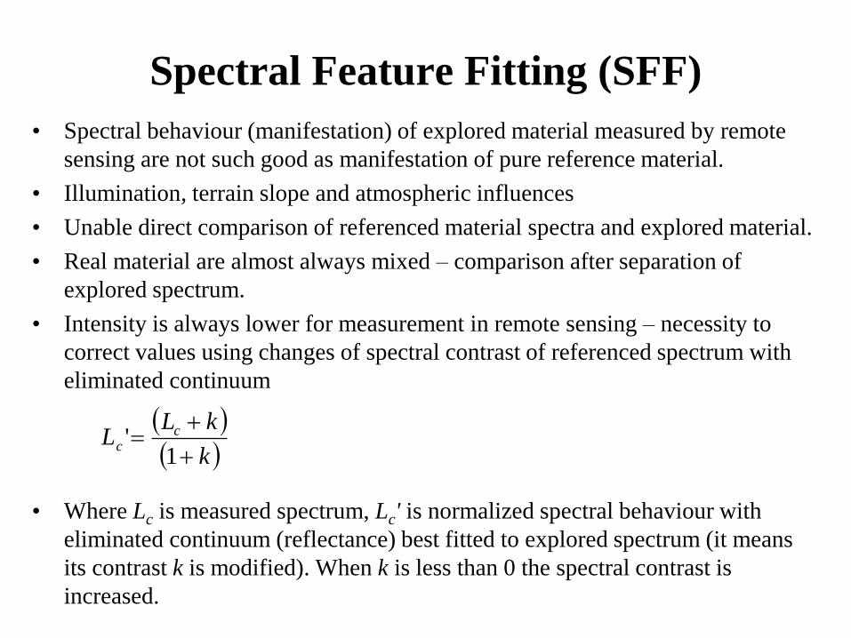
• Intensity is always lower for measurement in remote sensing – necessity to
correct values using changes of spectral contrast of referenced spectrum with
eliminated continuum
• Where Lc is measured spectrum, Lc' is normalized spectral behaviour with
eliminated continuum (reflectance) best fitted to explored spectrum (it means
its contrast k is modified). When k is less than 0 the spectral contrast is
increased.
k
kLL c
c
1'
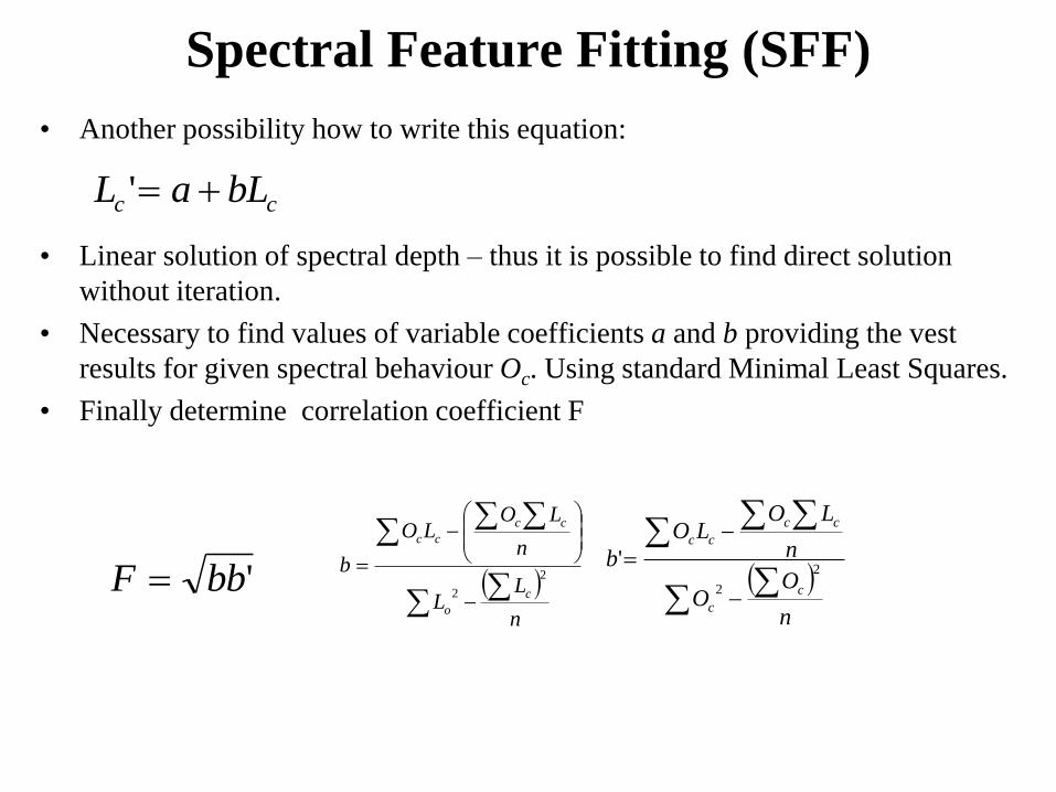
Spectral Feature Fitting (SFF)
• Another possibility how to write this equation:
• Linear solution of spectral depth – thus it is possible to find direct solution
without iteration.
• Necessary to find values of variable coefficients a and b providing the vest
results for given spectral behaviour Oc. Using standard Minimal Least Squares.
• Finally determine correlation coefficient F
cc bLaL '
'bbF
n
LL
n
LOLO
b
c
o
cc
cc
2
2
n
OO
n
LOLO
b
c
c
cc
cc
2
2
'
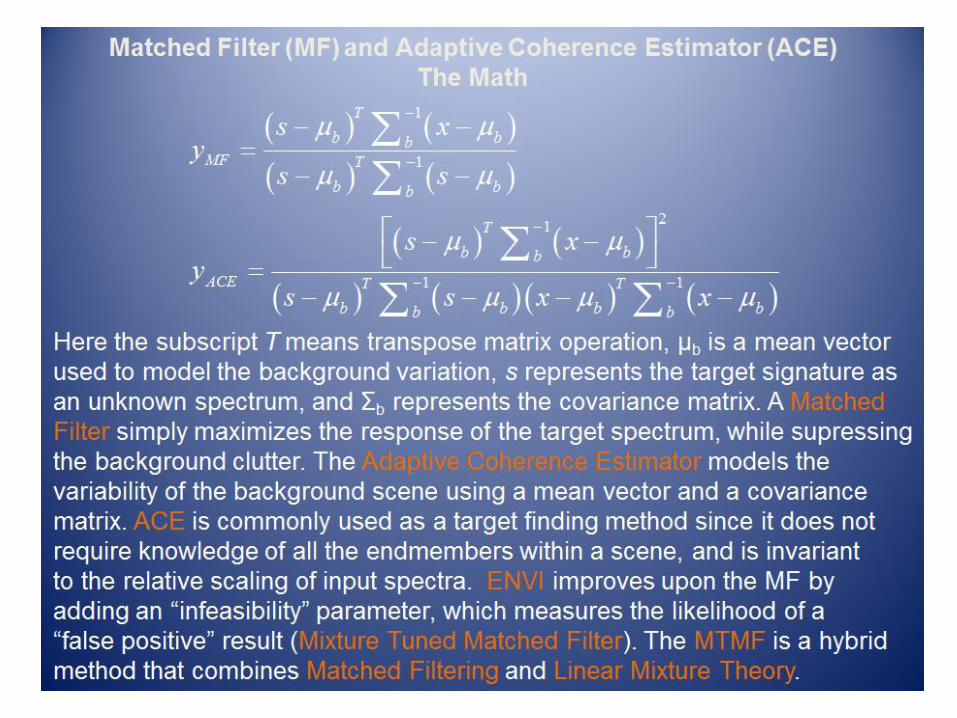
Adaptive Coherence Estimator (ACE)
• ACE models the background clutter using the data's statistics
(covariance matrix).
• ACE is commonly used as a target finding technique since
one does not have to have knowledge of all the endmembers
within a given scene, and because the method does not depend
on the relative scaling of input spectra
Mixture Tuned Matched Filter (MTMF)
• Combine MF technique and linear mixture theory.
• It contains infeasibility parameter which describes how
feasible is false positive error
• Useful mainly for sub-pixel analysis of material in the scene
• Method of analysis of heterogeneous pixels
• Suppose knowledge of:
– spectral profiles of each material
• Content of each material in the pixel in
percentage
• Measure of similarity between the spectral profile of investigated pixel and compared spectral profiles (end members)
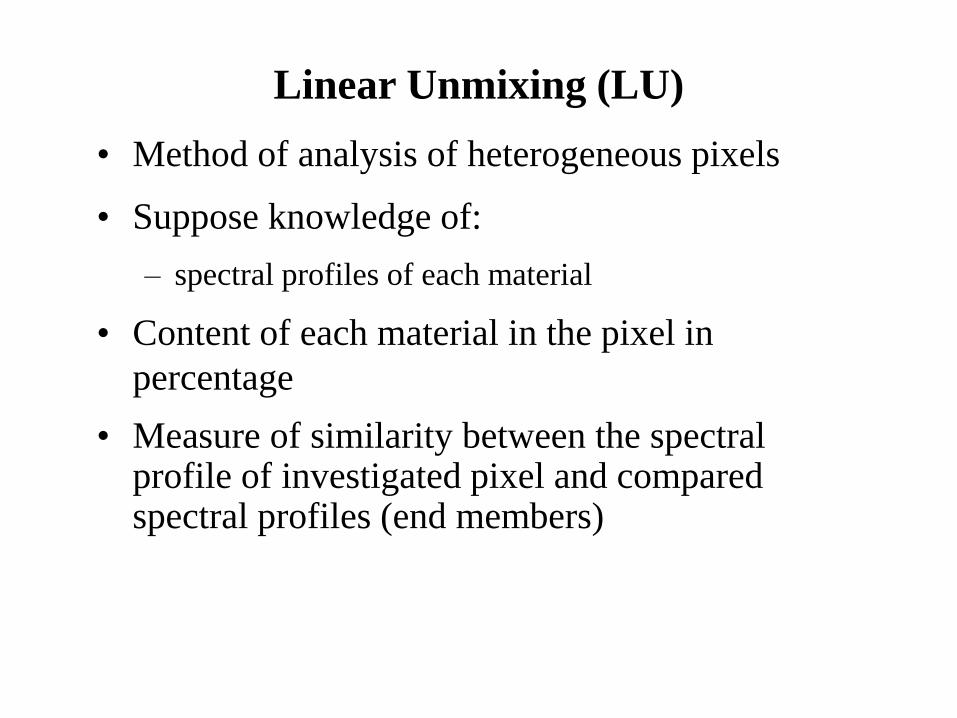
Linear Unmixing (LU)
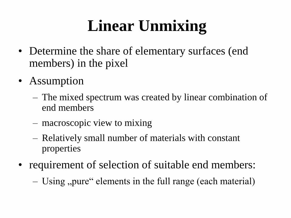
Linear Unmixing
• Determine the share of elementary surfaces (end members) in the pixel
• Assumption
– The mixed spectrum was created by linear combination of end members
– macroscopic view to mixing
– Relatively small number of materials with constant properties
• requirement of selection of suitable end members:
– Using „pure“ elements in the full range (each material)
Linear Unmixing (LU)
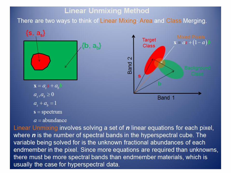
• Solve a system of N linear equation for each pixel (N is the number of spectral bands)
• Result is the abundance of each searched material in one pixel expressed as a share
• Ability to identify materials which are not able to distinguish in the image
• This is an example of what is known as "Non-literal" analysis, in contrast to literal analysis where objects are identified by eye.
Linear Unmixing (LU)
Linear Unmixing
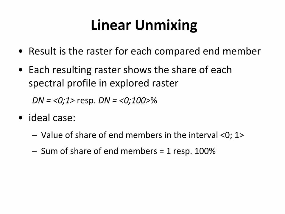
• Result is the raster for each compared end member
• Each resulting raster shows the share of each spectral profile in explored raster
DN = <0;1> resp. DN = <0;100>%
• ideal case:
– Value of share of end members in the interval <0; 1>
– Sum of share of end members = 1 resp. 100%
Evaluation of Linear Unmixing results
• Unsuitable parameters:
– Too much end members
– Unsuitable end members
• Sum of share of end members <> 1
• error raster – DN express:
– Residual error (RMS Error)
– high error values – low coincidence – necessity to include
more end members

Applications
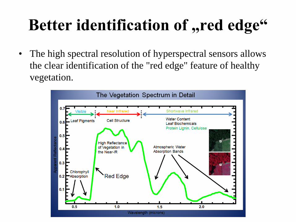
Better identification of „red edge“
• The high spectral resolution of hyperspectral sensors allows
the clear identification of the "red edge" feature of healthy
vegetation.
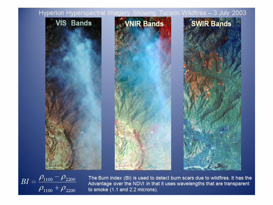
Burn index BI
• Mapping of burn scars and hot spots (seen as orange and
bright orange spots on the right image) through smoke
resulting from wildfires.
• The smoke is more transparent in the SWIR bands than in the
VNIR bands.
• Using a contrast ratio of two different SWIR bands, a Burn
Index (BI) can be created to measure the severity of burn
scars.
• Data Hyperion
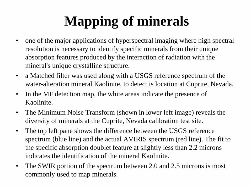
Mapping of minerals
• one of the major applications of hyperspectral imaging where high spectral
resolution is necessary to identify specific minerals from their unique
absorption features produced by the interaction of radiation with the
mineral's unique crystalline structure.
• a Matched filter was used along with a USGS reference spectrum of the
water-alteration mineral Kaolinite, to detect is location at Cuprite, Nevada.
• In the MF detection map, the white areas indicate the presence of
Kaolinite.
• The Minimum Noise Transform (shown in lower left image) reveals the
diversity of minerals at the Cuprite, Nevada calibration test site.
• The top left pane shows the difference between the USGS reference
spectrum (blue line) and the actual AVIRIS spectrum (red line). The fit to
the specific absorption doublet feature at slightly less than 2.2 microns
indicates the identification of the mineral Kaolinite.
• The SWIR portion of the spectrum between 2.0 and 2.5 microns is most
commonly used to map minerals.
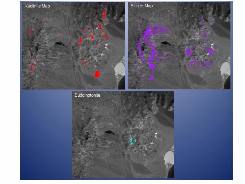
Mapping of minerals 2
• The following slide shows Matched Filter detections of three different
alteration minerals at the Cuprite, Nevada site.
• Kaolinite, Alunite, and Buddingtonite are shown as different color
overlays on top of a single baseline SWIR band.
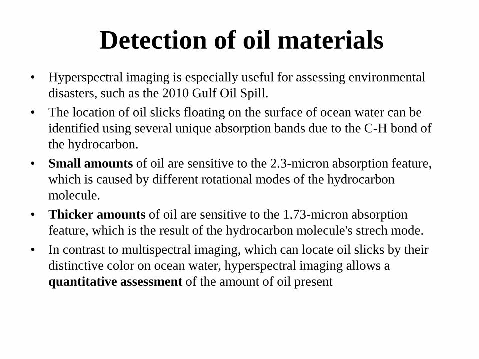
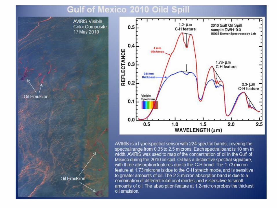
Detection of oil materials
• Hyperspectral imaging is especially useful for assessing environmental
disasters, such as the 2010 Gulf Oil Spill.
• The location of oil slicks floating on the surface of ocean water can be
identified using several unique absorption bands due to the C-H bond of
the hydrocarbon.
• Small amounts of oil are sensitive to the 2.3-micron absorption feature,
which is caused by different rotational modes of the hydrocarbon
molecule.
• Thicker amounts of oil are sensitive to the 1.73-micron absorption
feature, which is the result of the hydrocarbon molecule's strech mode.
• In contrast to multispectral imaging, which can locate oil slicks by their
distinctive color on ocean water, hyperspectral imaging allows a
quantitative assessment of the amount of oil present
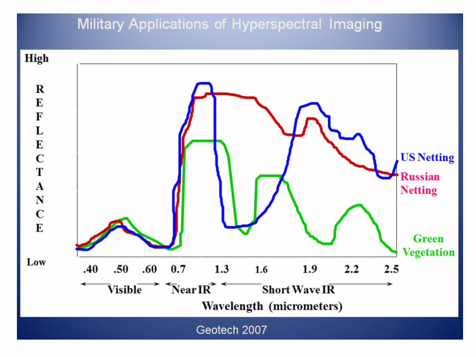
Military applications
• The high spectral resolution of hyperspectral sensors allows one
to discriminate not only camouflage from background
clutter, but different types of camouflage.
• Note the common spectral feature of two types of camouflage.
They all "mimic" the red edge of vegetation, so they would all
appear to blend in with background vegetation if they were
imaged using conventional NIR/Red/Green multispectral
imaging systems.
• However, hyperspectral imaging systems with expanded
spectral coverage in addition to higher spectral resolution can
differentiate the different types of camouflage, especially when
examined in the SWIR portion of the spectrum. The SWIR
bands also allow the discrimination between the two types of
camouflage and the background vegetation.
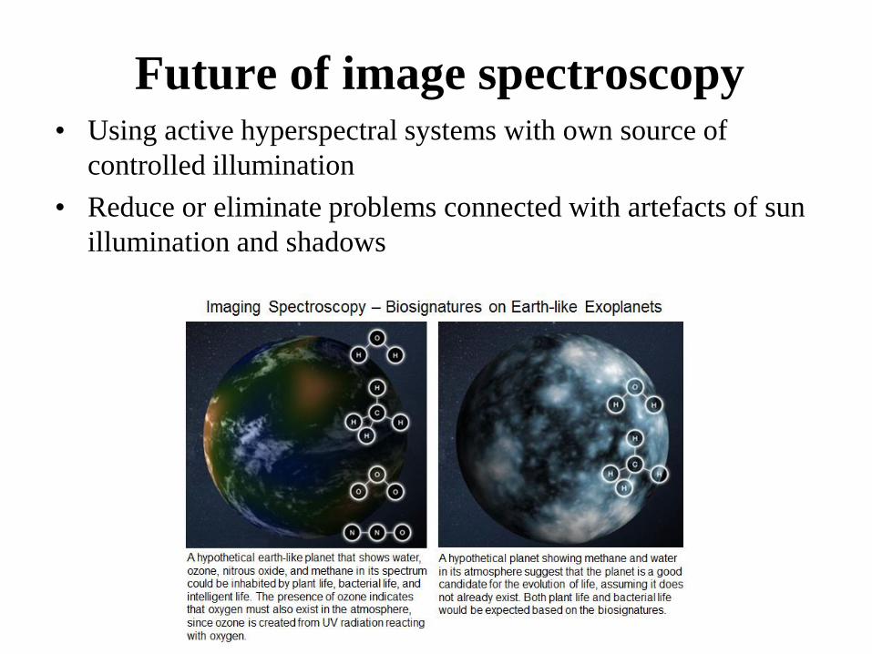
Future of image spectroscopy • Using active hyperspectral systems with own source of
controlled illumination
• Reduce or eliminate problems connected with artefacts of sun
illumination and shadows