Technische Universit�at Chemnitz-ZwickauSonderforschungsbereich 393Numerische Simulation auf massiv parallelen RechnernWolfgang Rehm (Ed.)Portierbare numerische Simulationauf parallelen ArchitekturenPreprint SFB393/96-07Einband der zum gleichnamigen Workshop erschienenenComputer Achitecture Technical Reportsdes Lehrstuhls Rechnerarchitektur/Informatik

Preprint-Reihe des Chemnitzer SFB 393SFB393/96-07 April 1996

ContentsPreface 1Benchmarking 2Architectural Development Tracks in Parallel Computing { A Brief Over-view 15Parallel FEM Implementations on Shared Memory Systems 24Leistungsvergleich ausgew�ahlter Funktionen verschiedener MPI-Imple-mentierungen 33Message Passing E�ciency on Shared Memory Architectures 63MPI-Portierung eines FEM-Programmes 75Application Oriented Monitoring 85An Implementation of MPI { The Shared Memory Device 99Principles of Parallel Computers and some Impacts on their Program-ming Models 115

PrefaceThe workshop \Portierbare numerische Simulationen auf parallelen Architekturen"(\Portable numerical simulations on parallel architectures") was organized by the Fac-ulty of Informatics/Professorship Computer Architecture at 18 April 1996 and held inthe framework of the Sonderforschungsbereich (Joint Research Initiative) \NumerischeSimulationen auf massiv parallelen Rechnern" (SFB 393) (\Numerical simulations onmassiv parallel computers") (http://www.tu-chemnitz.de/�pester/sfb/sfb393.html)The SFB 393 is funded by the German National Science Foundation (DFG).The purpose of the workshop was to bring together scientists using parallel computingto provide integrated discussions on portability issues, requirements and future devel-opments in implementing parallel software e�ciently as well as portable on Clusters ofSymmetric MultiprocessorsystemsI hope that the present paper gives the reader some helpful hints for further discussionsin this �eld.April 1996 Wolfgang Rehm

1

BenchmarkingSven Schindlersvsc@informatik.tu-chemnitz.dehttp://noah.informatik.tu-chemnitz.de/members/schindler/schindler.htmlZusammenfassungNach einer kurzen Erl�auterung theoretischer Grundlagen werden stellverte-tend die Benchmarks des Performance Database Servers sowie ein eigener Bench-mark vorgestellt.Im weiteren werden Theorie und Probleme des parallelen Bench-marking behandelt.1 Einf�uhrung1.1 HistorischesDer Begri� BENCHMARK tauchte erstmals 1840 bei nordamerikanischen Landver-messern auf. Er bezeichnet eine Erhebung, welche als fester Punkt zur Landvermessungverwendet wurde.Heute versteht man unter dem Begri� Benchmark einen Referenzpunkt, welcher dieLeistungsbestimmung von verschiedenen Rechnern erm�oglicht. Ein Beispiel f�ur einensolchen Referenzpunkt sind die 1-MIPS der VAX{11/780.Benchmarks sind ein wichtiges Hilfsmittel zur Leistungsbestimmung bzw. Leistungs-vorhersage von Rechnersystemen.1.2 Begri�eRuntime(Laufzeit):� Laufzeit eines Programm auf einem konkreten Rechner� bildet Grundlage zur bestimmung anderer Performancegr�o�enMIPS = Million Instructions Per SecondMFLOPS = Million Floating{Point Operations Per Second2

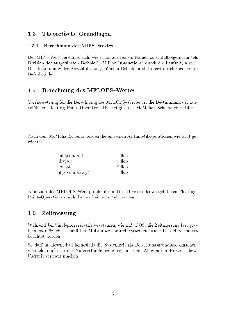
1.3 Theoretische Grundlagen1.3.1 Berechnung des MIPS{WertesDer MIPS{Wert berechnet sich, wie schon aus seinem Namen zu schlu�folgern, mittelsDivision der ausgef�uhrten Befehle(in Million Instructions) durch die Laufzeit(in sec).Die Bestimmung der Anzahl der ausgef�uhrten Befehle erfolgt meist durch sogenannteBefehlsz�ahler.1.4 Berechnung des MFLOPS{WertesVorraussetzung f�ur die Berechnung des MFLOPS{Wertes ist die Bestimmung der aus-gef�uhrten Floating{Point{Operations.Hierbei gibt das McMahon Schema eine Hilfe.Nach dem McMohanSchema werden die einzelnen Arithmetikoperationen wie folgt ge-wichtet: add,sub,mul 1 opdiv,sqr 4 opexp,sin ... 8 opif(x compare y) 1 opNun kann der MFLOPS{Wert problemlos mittels Division der ausgef�uhrten Floating{Point{Operations durch die Laufzeit ermittelt werden.1.5 ZeitmessungW�ahrend bei Singleprozessbetriebssystemen, wie z.B. DOS, die Zeitmessung fast pro-blemlos m�oglich ist mu� bei Multiprozessbetriebssystemen, wie z.B. UNIX, einigesbeachtet werden.So darf in diesem Fall keinesfalls die Systemzeit als Bewertungsgrundlage eingehen,vielmehr mu� sich der Nutzer(Implementierer) mit dem Ablesen der Prozess{ bzw.Userzeit vertraut machen. 3

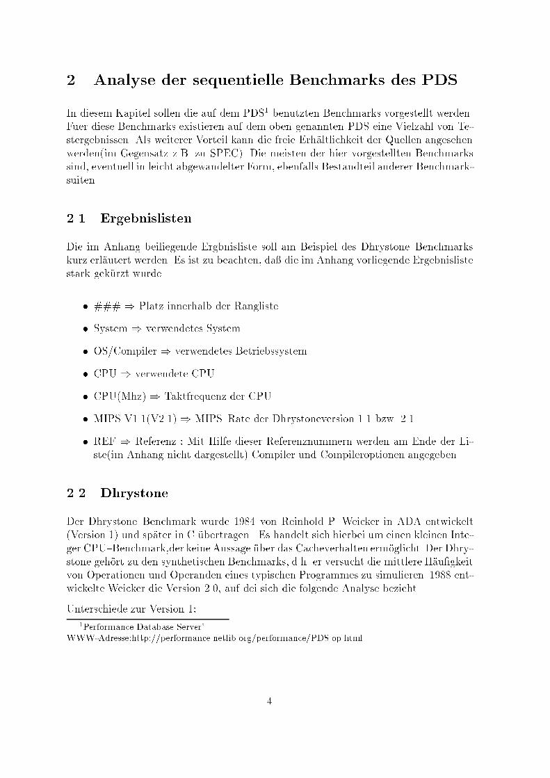
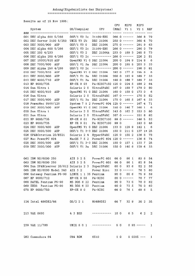
2 Analyse der sequentielle Benchmarks des PDSIn diesem Kapitel sollen die auf dem PDS1 benutzten Benchmarks vorgestellt werden.Fuer diese Benchmarks existieren auf dem oben genannten PDS eine Vielzahl von Te-stergebnissen. Als weiterer Vorteil kann die freie Erh�altlichkeit der Quellen angesehenwerden(im Gegensatz z.B. zu SPEC). Die meisten der hier vorgestellten Benchmarkssind, eventuell in leicht abgewandelter Form, ebenfalls Bestandteil anderer Benchmark-suiten.2.1 ErgebnislistenDie im Anhang beiliegende Ergbnisliste soll am Beispiel des Dhrystone{Benchmarkskurz erl�autert werden. Es ist zu beachten, da� die im Anhang vorliegende Ergebnislistestark gek�urzt wurde.� ###) Platz innerhalb der Rangliste� System) verwendetes System� OS/Compiler) verwendetes Betriebssystem� CPU ) verwendete CPU� CPU(Mhz) ) Taktfrequenz der CPU� MIPS V1.1(V2.1) ) MIPS{Rate der Dhrystoneversion 1.1 bzw. 2.1� REF ) Referenz : Mit Hilfe dieser Referenznummern werden am Ende der Li-ste(im Anhang nicht dargestellt) Compiler und Compileroptionen angegeben.2.2 DhrystoneDer Dhrystone{Benchmark wurde 1984 von Reinhold P. Weicker in ADA entwickelt(Version 1) und sp�ater in C �ubertragen . Es handelt sich hierbei um einen kleinen Inte-ger CPU{Benchmark,der keine Aussage �uber das Cacheverhalten erm�oglicht.Der Dhry-stone geh�ort zu den synthetischen Benchmarks, d.h. er versucht die mittlere H�au�gkeitvon Operationen und Operanden eines typischen Programmes zu simulieren. 1988 ent-wickelte Weicker die Version 2.0, auf dei sich die folgende Analyse bezieht.Unterschiede zur Version 1:1Performance Database Server'WWW-Adresse:http://performance.netlib.org/performance/PDS.op.html4

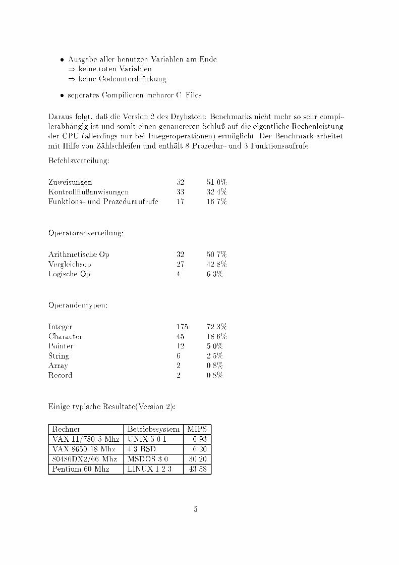
� Ausgabe aller benutzen Variablen am Ende) keine toten Variablen) keine Codeunterdr�uckung� seperates Compilieren meherer C{FilesDaraus folgt, da� die Version 2 des Dryhstone{Benchmarks nicht mehr so sehr compi-lerabh�angig ist und somit einen genauereren Schlu� auf die eigentliche Rechenleistungder CPU (allerdings nur bei Integeroperationen) erm�oglicht. Der Benchmark arbeitetmit Hilfe von Z�ahlschleifen und enth�alt 8 Prozedur- und 3 Funktionsaufrufe.Befehlsverteilung:Zuweisungen 52 51.0%Kontroll u�anwisungen 33 32.4%Funktions- und Prozeduraufrufe 17 16.7%Operatorenverteilung:Arithmetische Op. 32 50.7%Vergleichsop. 27 42.8%Logische Op. 4 6.3%Operandentypen:Integer 175 72.3%Character 45 18.6%Pointer 12 5.0%String 6 2.5%Array 2 0.8%Record 2 0.8%Einige typische Resultate(Version 2):Rechner Betriebssystem MIPSVAX 11/780 5 Mhz UNIX 5.0.1 0.93VAX 8650 18 Mhz 4.3 BSD 6.2080486DX2/66 Mhz MSDOS 3.0 30.20Pentium 60 Mhz LINUX 1.2.3 43.585

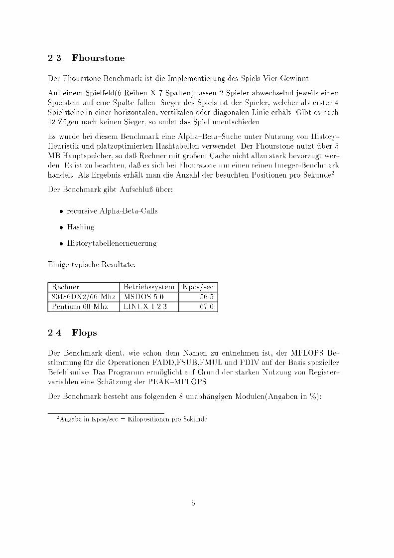
2.3 FhourstoneDer Fhourstone-Benchmark ist die Implementierung des Spiels Vier-Gewinnt.Auf einem Spielfeld(6 Reihen X 7 Spalten) lassen 2 Spieler abwechselnd jeweils einenSpielstein auf eine Spalte fallen. Sieger des Spiels ist der Spieler, welcher als erster 4Spielsteine in einer horizontalen, vertikalen oder diagonalen Linie erh�alt. Gibt es nach42 Z�ugen noch keinen Sieger, so endet das Spiel unentschieden.Es wurde bei diesem Benchmark eine Alpha{Beta{Suche unter Nutzung von History-Heuristik und platzoptimierten Hashtabellen verwendet. Der Fhourstone nutzt �uber 5MB Hauptspeicher, so da� Rechner mit gro�em Cache nicht allzu stark bevorzugt wer-den. Es ist zu beachten, da� es sich bei Fhourstone um einen reinen Integer-Benchmarkhandelt. Als Ergebnis erh�alt man die Anzahl der besuchten Positionen pro Sekunde2.Der Benchmark gibt Aufschlu� �uber:� recursive Alpha-Beta-Calls� Hashing� HistorytabellenerneuerungEinige typische Resultate:Rechner Betriebssystem Kpos/sec80486DX2/66 Mhz MSDOS 5.0 56.5Pentium 60 Mhz LINUX 1.2.3 67.62.4 FlopsDer Benchmark dient, wie schon dem Namen zu entnehmen ist, der MFLOPS{Be-stimmung f�ur die Operationen FADD,FSUB,FMUL und FDIV auf der Basis speziellerBefehlsmixe. Das Programm erm�oglicht auf Grund der starken Nutzung von Register-variablen eine Sch�atzung der PEAK{MFLOPS.Der Benchmark besteht aus folgenden 8 unabh�angigen Modulen(Angaben in %):2Angabe in Kpos/sec = Kilopositionen pro Sekunde6

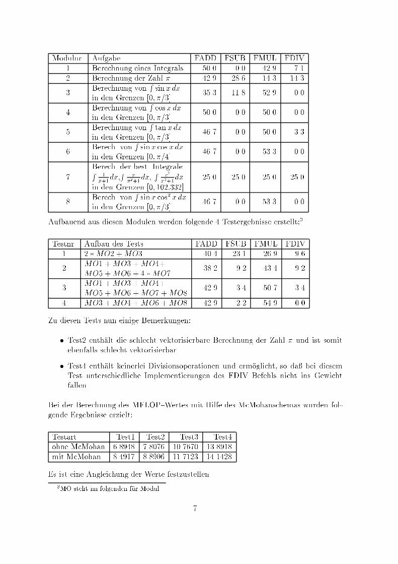
Modulnr. Aufgabe FADD FSUB FMUL FDIV1 Berechnung eines Integrals 50.0 0.0 42.9 7.12 Berechnung der Zahl � 42.9 28.6 14.3 14.3Berechnung von R sin x dx3 in den Grenzen [0; �=3] 35.3 11.8 52.9 0.0Berechnung von R cos x dx4 in den Grenzen [0; �=3] 50.0 0.0 50.0 0.0Berechnung von R tan x dx5 in den Grenzen [0; �=3] 46.7 0.0 50.0 3.3Berech. von R sinx cos x dx6 in den Grenzen [0; �=4] 46.7 0.0 53.3 0.0Berech. der best. Integrale7 R 1x+1dx,R xx2+1dx, R x2x3+1dx 25.0 25.0 25.0 25.0in den Grenzen [0; 102:332]Berech. von R sinx cos2 x dx8 in den Grenzen [0; �=3] 46.7 0.0 53.3 0.0Aufbauend aus diesen Modulen werden folgende 4 Testergebnisse erstellt:3Testnr. Aufbau des Tests FADD FSUB FMUL FDIV1 2 �MO2 +MO3 40.4 23.1 26.9 9.6MO1 +MO3 +MO4+2 MO5 +MO6 + 4 �MO7 38.2 9.2 43.4 9.2MO1 +MO3 +MO4+3 MO5 +MO6 +MO7 +MO8 42.9 3.4 50.7 3.44 MO3 +MO4 +MO6 +MO8 42.9 2.2 54.9 0.0Zu diesen Tests nun einige Bemerkungen:� Test2 enth�alt die schlecht vektorisierbare Berechnung der Zahl � und ist somitebenfalls schlecht vektorisierbar� Test4 enth�alt keinerlei Divisionsoperationen und erm�oglicht, so da� bei diesemTest unterschiedliche Implementierungen des FDIV Befehls nicht ins GewichtfallenBei der Berechnung des MFLOP{Wertes mit Hilfe des McMohanschemas wurden fol-gende Ergebnisse erzielt:Testart Test1 Test2 Test3 Test4ohne McMohan 6.8948 7.8076 10.7670 13.8918mit McMohan 8.4917 8.8906 11.7123 14.1428Es ist eine Angleichung der Werte festzustellen.3MO steht im folgenden f�ur Modul 7

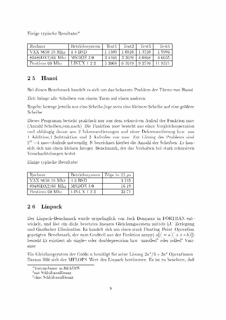
Einige typische Resultate:4Rechner Betriebssystem Test1 Test2 Test3 Test4VAX 8650 18 Mhz 4.3 BSD 1.1380 1.0810 1.3710 1.599480486DX2/66 Mhz MSDOS 3.0 3.4166 3.3628 4.0868 4.6655Pentium 60 Mhz LINUX 1.2.3 5.3068 6.7619 9.3710 11.95212.5 HanoiBei diesen Benchmark handelt es sich um das bekannte Problem der T�urme von Hanoi.Ziel: bringe alle Scheiben von einem Turm auf einen anderenRegeln: bewege jeweils nur eine Scheibe,lege stets eine kleinere Scheibe auf eine gr�o�ereScheibeDieses Programm besteht praktisch nur aus dem rekursiven Aufruf der Funktion mov(Anzahl Scheiben,von,nach). Die Funktion mov besteht aus einer Vergleichsoperationund abh�angig davon aus 2 Inkrementierungen und einer Dekrementierung bzw. aus1 Addition,1 Subtraktion und 3 Aufrufen von mov. Zur L�osung des Problems sind2N �1 mov{Aufrufe notwendig. N bezeichnet hierbei die Anzahl der Scheiben. Es han-delt sich um einen kleinen Integer{Benchmark, der das Verhalten bei stark rekursivenVerschachtelungen testet.Einige typische Resultate:Rechner Betriebssystem Z�uge in 25 �sVAX 8650 18 Mhz 4.3 BSD 3.74580486DX2/66 Mhz MSDOS 3.0 16.19Pentium 60 Mhz LINUX 1.2.3 33.712.6 LinpackDer Linpack{Benchmark wurde urspr�unglich von Jack Dongarra in FORTRAN ent-wickelt, und l�ost ein dicht besetztes lineares Gleichungssystem mittels LU{Zerlegungund Gau�scher Elimination. Es handelt sich um einen stark Floating{Point{Operationgepr�agten Benchmark, der zum Gro�teil aus der Funktion saxpy( a[i] = a[i] + x � b[i])besteht.Er existiert als single{ oder doubleprecision bzw. unrolled5 oder rolled6 Vari-ante.Ein Gleichungsystem der Gr�o�e n ben�otigt f�ur seine L�osung 2n3=3 + 2n2 Operationen.Daraus l�a�t sich der MFLOPS{Wert des Linpack bestimmen. Es ist zu beachten, da�4Testergebnisse in MFLOPS5mit Schleifenau �osung6ohne Schleifenau �osung 8

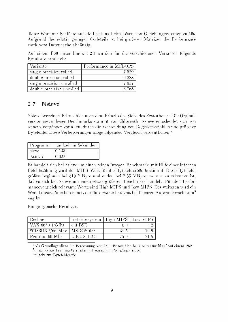
dieser Wert nur Schl�usse auf die Leistung beim L�osen von Gleichungssytemen zul�a�t.Aufgrund des relativ geringen Codeteils ist bei gr�o�eren Matrizen die Performancestark vom Datencache abh�angig.Auf einem P60 unter Linux 1.2.3 wurden f�ur die verschiedenen Varianten folgendeResultate ermittelt:Variante Performance in MFLOPSsingle precision rolled 7.529double precision rolled 6.288single precision unrolled 7.957double precision unrolled 6.7652.7 NsieveNsieve berechnet Primzahlen nach dem Prinzip des Siebs des Eratothenes. Die Orginal-version sieve dieses Benchmarks stammt von Gilbreath. Nsieve entscheidet sich vonseinem Vorg�anger vor allem durch die Verwendung von Registervariablen und gr�o�ererBytefelder.Diese Verbesserungen m�oge folgender Vergleich verdeutlichen:7Programm Laufzeit in Sekundensieve 0.133Nsieve 0.022Es handelt sich bei nsieve um einen reinen Integer{Benchmark. mit Hilfe einer internenBefehlsz�ahlung wird der MIPS{Wert f�ur die Bytefeldgr�o�e bestimmt. Diese Bytefeld-gr�o�en beginnen bei 81918 Byte und enden bei 2.56 MByte, woraus zu erkennen ist,da� es sich bei Nsieve um einen etwas gr�o�eren Benchmark handelt. F�ur den Perfor-mancevergleich relevante Werte sind High MIPS und Low MIPS. Des weiteren wird einWert Linear Time berechnet, der die erwarte Laufzeit bei linearen Aufwandswachstum9angibt.Einige typische Resultate:Rechner Betriebssystem High MIPS Low MIPSVAX 8650 18Mhz 4.3 BSD 6.0 3.280486DX2/66 Mhz MSDOS 6.0 34.5 19.9Pentium 60 Mhz LINUX 1.2.3 75.0 31.57Als Grundlage dient die Berechnung von 1899 Primzahlen bei einem Durchlauf auf einem P608dieser etwas krumme Wert stammt von seinem Vorg�anger sieve9relativ zur Bytefeldgr�o�e 9

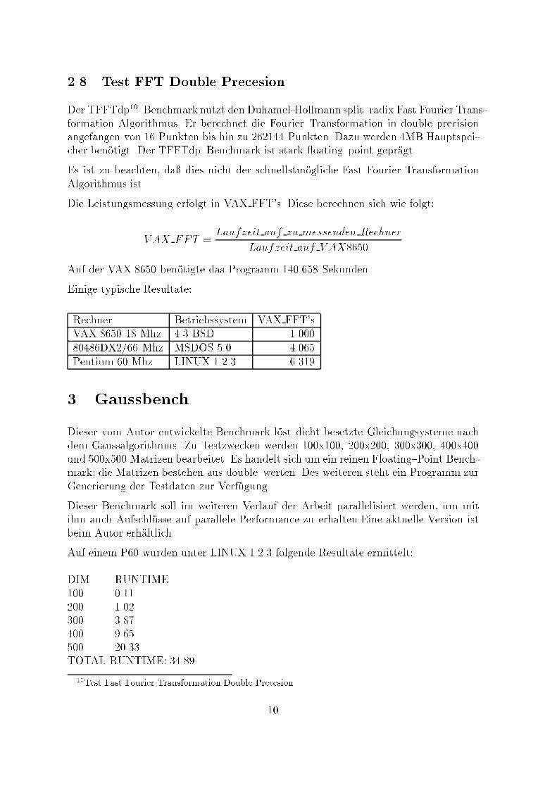
2.8 Test FFT Double PrecesionDer TFFTdp10{Benchmark nutzt den Duhamel-Hollmann split{radix Fast Fourier Trans-formation Algorithmus. Er berechnet die Fourier{Transformation in double precisionangefangen von 16 Punkten bis hin zu 262144 Punkten. Dazu werden 4MB Hauptspei-cher ben�otigt. Der TFFTdp{Benchmark ist stark oating{point gepr�agt.Es ist zu beachten, da� dies nicht der schnellstm�ogliche Fast Fourier TransformationAlgorithmus ist.Die Leistungsmessung erfolgt in VAX FFT's. Diese berechnen sich wie folgt:V AX FFT = Laufzeit auf zu messenden RechnerLaufzeit auf V AX8650Auf der VAX 8650 ben�otigte das Programm 140.658 Sekunden.Einige typische Resultate:Rechner Betriebssystem VAX FFT'sVAX 8650 18 Mhz 4.3 BSD 1.00080486DX2/66 Mhz MSDOS 5.0 4.065Pentium 60 Mhz LINUX 1.2.3 6.3193 GaussbenchDieser vom Autor entwickelte Benchmark l�ost dicht besetzte Gleichungsysteme nachdem Gaussalgorithmus. Zu Testzwecken werden 100x100, 200x200, 300x300, 400x400und 500x500 Matrizen bearbeitet. Es handelt sich um ein reinen Floating{Point Bench-mark; die Matrizen bestehen aus double{werten. Des weiteren steht ein Programm zurGenerierung der Testdaten zur Verf�ugung.Dieser Benchmark soll im weiteren Verlauf der Arbeit parallelisiert werden, um mitihm auch Aufschl�usse auf parallele Performance zu erhalten.Eine aktuelle Version istbeim Autor erh�altlich.Auf einem P60 wurden unter LINUX 1.2.3 folgende Resultate ermittelt:DIM RUNTIME100 0.11200 1.02300 3.87400 9.65500 20.33TOTAL RUNTIME: 34.8910Test Fast Fourier Transformation Double Precesion10

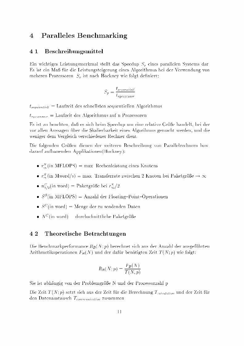
4 Paralleles Benchmarking4.1 BeschreibungsmittelEin wichtiges Leistungsmerkmal stellt das Speedup Sp eines parallelen Systems dar.Es ist ein Ma� f�ur die Leistungsteigerung eines Algorithmus bei der Verwendung vonmeheren Prozessoren. Sp ist nach Hockney wie folgt de�niert:Sp = tsequentielltnprocessortsequientiell = Laufzeit des schnellsten sequentiellen Algorithmustnprocessor = Laufzeit des Algorithmus auf n ProzessorenEs ist zu beachten, da� es sich beim Speedup um eine relative Gr�o�e handelt, bei dervor allen Aussagen �uber die Skalierbarkeit eines Algorihmus gemacht werden, und dieweniger dem Vergleich verschiedener Rechner dient.Die folgenden Gr�o�en dienen der weiteren Beschreibung von Parallelrechnern bzw.darauf aufbauenden Applikationen(Hockney):� rS1(in MFLOPS) = max. Rechenleistung eines Knotens� rS1(in Mword/s) = max. Transferrate zwischen 2 Knoten bei Paketgr�o�e !1� nC1=2(in word) = Paketgr�o�e bei rS1=2� SS(in MFLOPS) = Anzahl der Floating{Point{Operationen� SC(in word) = Menge der zu sendenden Daten� NC(in word) = durchschnittliche Paketgr�o�e4.2 Theoretische BetrachtungenDie Benchmarkperformance RB(N ; p) berechnet sich aus der Anzahl der ausgef�uhrtenArithmetikoperationen FB(N) und der daf�ur ben�otigten Zeit T (N ; p) wie folgt:RB(N ; p) = FB(N)T (N; p)Sie ist abh�angig von der Problemgr�o�e N und der Prozessorzahl p.Die Zeit T (N ; p) setzt sich aus der Zeit f�ur die Berechnung Tcalculation und der Zeit f�urden Datenaustausch Tcommunication zusammen.11

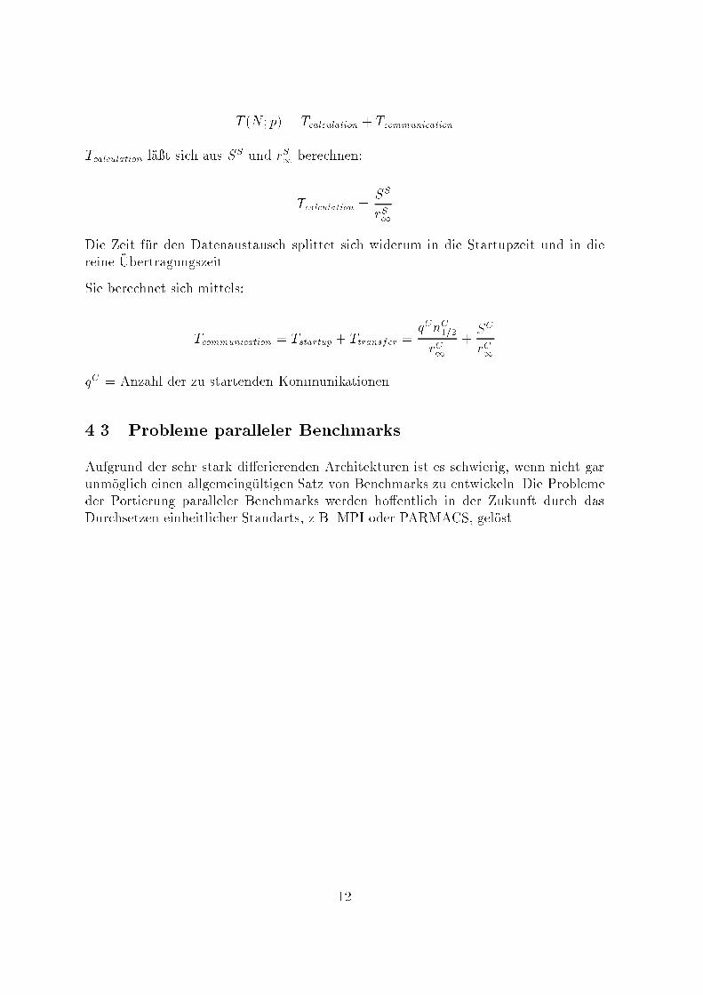
T (N ; p) = Tcalculation + TcommunicationTcalculation l�a�t sich aus SS und rS1 berechnen:Tcalculation = SSrS1Die Zeit f�ur den Datenaustausch splittet sich widerum in die Startupzeit und in diereine �Ubertragungszeit.Sie berechnet sich mittels:Tcommunication = Tstartup + Ttransfer = qCnC1=2rC1 + SCrC1qC = Anzahl der zu startenden Kommunikationen.4.3 Probleme paralleler BenchmarksAufgrund der sehr stark di�erierenden Architekturen ist es schwierig, wenn nicht garunm�oglich einen allgemeing�ultigen Satz von Benchmarks zu entwickeln. Die Problemeder Portierung paralleler Benchmarks werden ho�entlich in der Zukunft durch dasDurchsetzen einheitlicher Standarts, z.B. MPI oder PARMACS, gel�ost.

12

Literatur[DON95] Jack J. Dongarra : Performance of Various Computers Using Standart LinearEquations Software[HOC88] Roger W. Hockney, Cristo�er R. Jesshope: Architecture, Programming andAlgorithmnsAdam Hilger/IOP Publishing, Bristol & Philadelphia[HOC94] Roger W. Hockney : Performance Parameters and Results for the GenesisParallel BenchmarksPortability and Performance for Parallel Processing , John Wiley & Sons[HP90] John L. Hennessy, David L. Patterson : Computer Architecture : A Quanti-tative ApproachMorgan Kaufmann Publishers, Inc., San Mateo, California[KLE94] Andreas Kleber: Entwicklung,Implementierung und Evaluierung eines paral-lelen Benchmarksatzes f�ur DM{MIMD{Rechner[LAR93] Brian Howard LaRose: The Development and Implementation of a Perfor-mance Database ServerComputer Science Department CS-93-195[WEI84] Reinhold P. Weicker: Dhystone: A Synthetic Systems Programming Bench-markComm. ACM 27,10[WEI88] Reinhold P. Weicker: Dhrystone Benchmark: Rationale for Version 2 andMeasurement RulesSIGPLAN Notices vol. 23 no. 813

Anhang(Ergebnisliste des Dhrystone)========================================Results as of 15 Nov 1995: CPU MIPS MIPSSystem OS/Compiler CPU (MHz) V1.1 V2.1 REF### ---------------------- ------------ ----------- ----- ------ ------ ---001 DEC Alpha 600 5/266 OSF/1 V3.2c 21164-EB5 266.0 ------ 366.8 79002 DEC Server 2100 5/250 UNIX V3.2b DEC 21064 250.0 ------ 360.4 70003 DEC 3000/900 AXP OSF/1 V3.0 DEC 21064 275.0 ------ 291.9 63004 DEC Alpha 600 5/266 OSF/1 V3.2c 21164-EB5 266.0 ------ 290.0 79005 DEC 200 4/233 OSF/1 V3.2 DEC 21064A 233.0 189.3 245.8 73006 DEC Alpha 250 4/266 OSF/1 V3.2c ----------- 266.0 ------ 226.2 81007 DEC 10000/610 AXP OpenVMS V1.0 DEC 21064 200.0 194.9 214.8 6008 DEC 7000/600 AXP OSF/1 V1.3a DEC 21064 200.0 195.5 203.3 33009 DEC Alpha 250 4/266 OSF/1 V3.2c ----------- 266.0 ------ 196.0 81010 DEC 7000/610 AXP OpenVMS V1.0 DEC 21064 182.0 177.3 195.6 6011 DEC 3000/800 AXP OSF/1 V1.3a DEC 21064 200.0 192.9 189.7 33012 DEC 4000/710 AXP OSF/1 V1.3a DEC 21064 190.0 188.7 189.7 33013 HP 9000/735 HP-UX 9.03 PA-RISC7150 125.0 224.5 189.2 64014 Sun Ultra 1 Solaris 2.5 UltraSPARC 167.0 189.7 179.0 80015 DEC 4000/610 AXP OpenVMS V1.0 DEC 21064 160.0 159.0 173.0 6016 Sun Ultra Solaris 2.5 UltraSPARC 167.0 ------ 170.8 82017 DEC 3000/600 AXP OSF/1 V1.3a DEC 21064 175.0 168.5 167.4 33018 PowerMac 9500/120 System 7.5.2 PowerPC 604 125.0 ------ 167.4 71019 DEC 3000/500 AXP OpenVMS V1.0 DEC 21064 150.0 146.7 160.1 6020 Sun Ultra 1 Solaris 2.5 UltraSPARC 143.0 162.2 153.0 80021 Sun Ultra Solaris 2.5 UltraSPARC 167.0 ------ 151.8 82022 HP 9000/735 HP-UX 9.01 PA-RISC7100 99.0 ------ 146.5 52023 HP 9000/735 HP-UX 9.01 PA-RISC7100 99.0 ------ 143.0 46024 DEC 3000/400 AXP OpenVMS V1.0 DEC 21064 133.0 129.9 142.1 6025 DEC 3000/500 AXP OSF/1 T1.3-3 DEC 21064 150.0 211.0 137.1* 25026 SPARCstation 20/HS21 Solaris 2.4 HyperSPARC 125.0 150.2 136.8 78027 Mac PowerPC 604 MacOS 7.5.2 PowerPC 604 120.0 ------ 136.6 74028 DEC 3000/500 AXP OSF/1 T1.3-3 DEC 21064 150.0 157.1 133.7 25029 DEC 2000/300 AXP OSF/1 V1.3a DEC 21064 150.0 140.9 129.4 33. . . . . . . .. . . . . . . .062 IBM RS/6000 250 AIX 3.2.5 PowerPC 601 66.0 96.1 83.6 54063 IBM RS/6000 250 AIX 3.2.5 PowerPC 601 66.0 96.1 82.8 54064 Sun SPARCserver 20/612 Solaris 2.3 SuperSPARC 60.0 93.6 82.2 58065 IBM RS/6000 Model 340 AIX 3.2 Power Risc 33.0 ------ 76.3 60066 Gateway Pentium P5-90 LINUX 1.1.35 Pentium 90.0 80.6 75.9 59067 HP 9000/712 HP-UX 9.05 PA-RISC 80.0 ------ 70.7 77068 DATEL Pentium P5-90 MS DOS 6.22 Pentium 90.0 73.0 70.0 62069 ZEOS Pentium P5-90 MS DOS 6.22 Pentium 90.0 72.5 70.0 62070 HP 9000/750 HP-UX 9.0 PA-RISC 66.0 76.1 69.6 5. . . . . . . .. . . . . . . .124 Intel 486DX2/66 OS/2 2.1 80486DX2 66.7 32.9 30.2 35. . . . . . . .. . . . . . . .213 VAX 8650 4.3 BSD ----------- 18.0 6.3 6.2 2. . . . . . . .. . . . . . . .239 VAX 11/780 UNIX 5.0.1 ----------- 5.0 0.93 ----- 1. . . . . . . .. . . . . . . .282 Commodore 64 C64 ROM 6510 1.0 0.0205 --- 1

Architectural Development Tracks in ParallelComputing { A Brief OverviewWolfgang Rehmrehm@informatik.tu-chemnitz.dehttp://noah.informatik.tu-chemnitz.de/members/rehm/rehm.htmlAbstractRecent results in parallel computing con�rm that highly parallel, general-purpose shared-memory computers can in principle be built. The architecturaldevelopment tracks follow no simple foreseeable path. This paper gives a briefoverview about some architectures have been recently emerged.1 IntroductionIn spite of the tremendous increase in computing power in the last years, nobody hasever felt a glut in computing power. The main technique computer architects are usingto achieve speedup is to do parallel processing.The parallism present in programs can be classi�ed into di�erent types - regular (dataparallelism) versus irregular, coarse-grain versus �ne-grain (instruction level) paral-lelism, etc. Coarse grain parallelism refers to the parallelism between large sets ofoperations such as subprograms, and is best exploited by multiprocessor systems.The key open architectural question is the nature of a parallel architecture �tting besta wide range of applications.Everybody should recognize the importance of what is called \mapping of problemarchitecture (spatio-temporal data access and communication patterns)" for gettingan e�cient implementation on a certain parallel computer architecture.Parallel systems encompass a full spectrum of size and prizes, from a collection ofworkstations that happen to be attached to the same local-area network, to an ex-pensive high-performance machine with hundreds or thousands of CPUs connected byultra-high-speed switches.Obviously, the speed and capacity of the CPUs and their communication medium con-strain the performance of any application. But from the perspective of the programmer,the way in which the multiple CPUs are controlled and the way they share informationmay have even more impact, in uencing not just the ultimate performance results butalso the level of e�ort needed to parallize an application.15

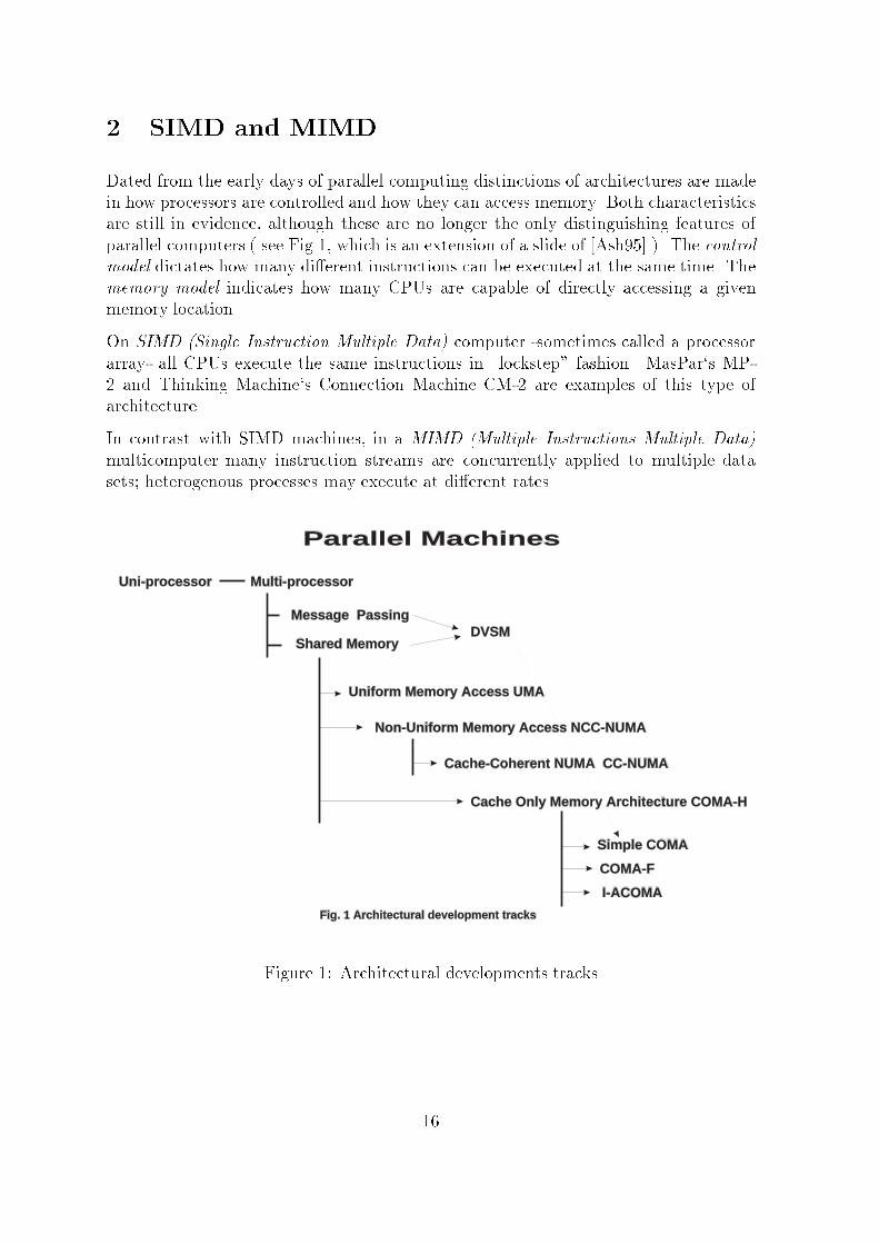
2 SIMD and MIMDDated from the early days of parallel computing distinctions of architectures are madein how processors are controlled and how they can access memory. Both characteristicsare still in evidence, although these are no longer the only distinguishing features ofparallel computers ( see Fig.1, which is an extension of a slide of [Ash95].). The controlmodel dictates how many di�erent instructions can be executed at the same time. Thememory model indicates how many CPUs are capable of directly accessing a givenmemory location.On SIMD (Single Instruction Multiple Data) computer -sometimes called a processorarray- all CPUs execute the same instructions in \lockstep" fashion. MasPar`s MP-2 and Thinking Machine`s Connection Machine CM-2 are examples of this type ofarchitecture.In contrast with SIMD machines, in a MIMD (Multiple Instructions Multiple Data)multicomputer many instruction streams are concurrently applied to multiple datasets; heterogenous processes may execute at di�erent rates.Parallel Machines

Uni-processor Multi-processor

Message Passing

Shared MemoryDVSM

Uniform Memory Access UMA

Non-Uniform Memory Access NCC-NUMA

Cache-Coherent NUMA CC-NUMA

Cache Only Memory Architecture COMA-H

Simple COMA

COMA-F

I-ACOMA

Fig. 1 Architectural development tracksFigure 1: Architectural developments tracks16

3 Shared Memory and Distributed MemoryOn a shared-memory multicomputer, the CPUs interact by accessing memory locationsin a single, shared address space. Traditional supercomputers (e.g. Cray Y/MP andC-90, IBM ES/9000, and Fujitsu Vector Processor Series) and the recently emergingso-called symmetric multiprocessor systems ( SMPs at the market place are e.g. 4-CPUSUN-Hypersparc, 4-12-CPU DEC Alpha Server, 16-30-CPU SGI PowerChallenge Line)are examples of this approach.On distributed-memory multicomputers, as the name implies, there is no shared mem-ory. Each CPU has a private memory and executes ist own instruction stream. Mostcurrent high-performance paralllel machines -due to their high processor count alsorefered as massively parallel processors (MPPs)- are of this type, e.g. Cray T3E, IBMSP-2, and Meiko CS-2. Since they are based on workstation microprocessors technol-ogy, these systems are versatile and very cost-e�ective. From some point of achitecturalview they are close related to so-called network of workstations (NOWs).4 Message Passing and Shared MemoryParallel computing on NOWs, also referred as workstations clusters (WSCs), has beengaining more attention in recent years. Because such workstation clusters use \of-the-shelf" products, they are cheaper than supercomputers. Furthermore, very powerfulworkstation processors and high-speed general-purpose networks are narrowing the per-formance gap between workstation clusters and supercomputers. All communication insuch a system must be performed by explicitly sending and receiving messages over thenetwork, since no physical memory is shared. This is too one reason why currently theprevailing programming model for parallel computing is message passing and a widelyaccepted message passing standard (library) MPI (Message Passing Inerface) [MPI93]has been developed and is still under development.Message-passing communication as well as shared-memory communication style viashared data structures are the major paradigms for parallel programming and, indeed,di�erent schools of thought. Each method has ist own strengths and shortcomings.Message passing seems to be more convenient for distributed-memory-type computersand shared-memory-type communication more convenient for multiprocessor systemswith a \naturally" global shared memory.I believe, that any programmingmodel that relies entirely on message passing or sharedmemory communication is very likely to fail because of inherent limitations of both.Instead of providing complete solutions for communication, providing simple RISC-like primitives, which expose the full range of hardware communication facilities (andthus the full hardware performance) to higher layers, will be a future solution to thiscontroversy (see also the Active Message approach).17

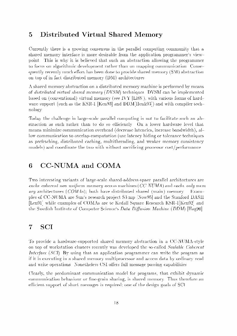
5 Distributed Virtual Shared MemoryCurrently there is a growing consensus in the parallel computing community that ashared memory interface is more desirable from the application programmer`s view-point. This is why it is believed that such an abstraction allowing the programmerto focus on algorithmic development rather than on mapping communication. Conse-quently recently much e�ort has been done to provide shared memory (SM) abstractionon top of in fact distributed memory (DM) architectures.A shared memory abstraction on a distributed memorymachine is performed by meansof distributed virtual shared memory (DVSM) techniques. DVSM can be implementedbased on (conventional) virtual memory (see IVY [Li88]), with various forms of hard-ware support (such as the KSR-1 [Ken93] and DDM[Henk93]) and with compiler tech-nology.Today the challenge in large-scale parallel computing is not to facilitate such an ab-straction as such rather than to do so e�ciently. On a lower hardware level thatmeans minimize communication overhead (decrease latencies, increase bandwidth), al-low communication to overlap computation (use latency hiding or tolerance techniquesas prefetching, distributed caching, multithreading, and weaker memory consistencymodels) and coordinate the two with without sacri�cing processor cost/performance.6 CC-NUMA and COMATwo interesting variants of large-scale shared-address-space parallel architectures arecache-coherent non-uniform-memory-access machines (CC-NUMA) and cache-only mem-ory architectures (COMAs); both have distributed shared (main) memory . Exam-ples of CC-NUMA are Sun`s research project S3.mp [Now95] and the Stanford DASH[Len91] while examples of COMAs are te Kedall Square Research KSR-1[Ken92] andthe Swedish Institute of Computer Science`s Data Di�usion Machine (DDM) [Hag90].7 SCITo provide a hardware-supported shared memory abstraction in a CC-NUMA-styleon top of workstation clusters recently was developed the so-called Scalable CoherentInterface (SCI). By using that an application programmer can write the program asif it is executing in a shared memory multiprocessor and access data by ordinary readand write operations. Nonetheless CSI o�ers full message passing capabilities.Clearly, the predominant communication model for programs, that exhibit dynamiccommunication behaviour or �ne-grain sharing, is shared memory. Thus therefore ane�cient support of short messages is required; one of the design goals of SCI.18

On the other hand the advantages of using message-passing over shared memory forcertain types of communication is an undisputed fact. That is why one can noticethat message passing machines are moving to e�cient support short messages anduniform address space and vice versa DSM computer are starting to provide supportfor message-like block transfer (SCI too).There is a convergence of both architectures in hardware and software mechanismto implement the communication abstarctions. A research projact dedicated to e�-cient integration and support of both cache coherent shared memory and low-overheaduser-level message passing is the FLASH (FLexible Architecture for Shared memory)multiprocessor [Kus94].8 SMPSo-called symmetric multiprocessor (SMP) machines are a recent addition to the par-allel computing marketplace. They also use workstation microprocessor technologybut additionaly join a small number of CPUs (typically 4, 8 or some more up to 30)with certain level of memory hierarchy, e.g. on the main memory level or/and onsecond-level caches, to achieve more power than high-end uniprocessor workstationso�er. Examples include Suns`s SPARCServer, HP/Convex`s Exemplar , and SGI`sPowerChallenge lines.In a typical simple structure all processors share a global memory via a common bus.If all processors additionaly have the same access capabilities to all I/O (interrupt)resources such a SMP is called symmetric. The cache-coherence problem can easily behandled by a bus-snooping protocol. Another advantage of a SMP is that all processeshave equal access time to shared (main) memory .That is why this architecture is calleda uniform memory-access (UMA) architecture. The main drawback of an SMP is therestricted scalibility due to the limited bandwidth of the common bus, which must beshared by all processors.9 SMP-ClusterA simple strategy for implementing a scalable and high-performance compuing facilityis to cluster SMPs, that means to build SMP-cluster (SMPC), via very high speedcommunication systems, e.g. like HIPPI switches or SCI interfaces. The resultingcon�guration behaves much like a distributed-memory multicomputer, exept that eachnode actually has multiple CPUs sharing a common memory.The problem arises with the emergence of SMPCs is how to program them. To date,the major performance success have been scored by programmers who treat SMPCsexactly as what they are: a collection of distinct, smal-scale shared-memeory systems.The communication within a SMP is carried out via shared memory (variables) andbetween SMPs by message passing. 19

To exploit parallelism within a SMP an appropriate programming model is that ofusing the abstraction of threads additionaly to processes (tasks). Whereas the threads(of a process) can only communicate via shared variables processes are able to useother communication primitives, particularly message passing. Remote process com-munication is restricted to message passing if no technology to provide global memoryaddressing is available. This is why a programmer must take care how to partitioningand communication is established for a special machine.Handling di�erent parallelism (processes, threads) and communication styles (sharedmemory, message passing) depending on the machine con�guration is an unacceptableway for a programmers view.One solution seems to take thoroughly a at paradigm of concurrent processes each onewith his own local memory communicating by messages. A more elaborated versionenables a hierachy in the sense that on the upper level appear only processes (e.g.the tasks with ports like in the MACH kernel) and downwards a process can containseveral threads of control. The threads of a process communicate via the process-localmemory, threads of di�erent processes have to use the communication surface of aprocess (e.g. ports). Both paradigms are convenient for SMPCs although the lattermakes changes in partitioning of parallel units more complicated.10 UMA, NUMA and COMAHowever, probably the primary issue for portable parallel programming (beside uniformaccess to the secondary storage system) is the to provide uniform access to memory.One of several software approaches to this problem is the experimental compiler Split-C from the University of California Berkeley; which is a parallel extension of the Claguage that supports access to a global address space on distributed multiprocessors.From the viepoint of a computer architect the main issue in maintain the abstractionof a global shared memory is the e�ective design of a DVSM.SMPCs with a DVSM are a prototype of an architecture where the memory accesstimes varying depending on if a local or a remote access (between SMPs) is performed.Such architectures are callednon uniform memeory access (NUMA) machines.Typically DSVM systems reqiure additionaly to the maintainance of the consistency ofcache-copies in the memory hierarchy of one node to maintain the coherence of multiplecache copies among caches of di�erent nodes (clusters of SMP). A basic concept ofcache coherence uses directory-based protocols. Machines as described are called cache-coherent non-uniform-memory-access (CC-NUMA) architectures. In contrast NUMAswith no cache-coherence support are called NCC-NUMAs.Beneath the variants of large-scale shared-address-space architectures are cache-onlymemory architectures (COMAs) an interesting solution.20

Both the CC-NUMA and the COMA type have distributed main memory and usedirectory-based cache coherence. Both too migrate and replicate data at the cachelevel automatically under hardware control, but COMAs do this at the main memorylevel as well. In a special sense COMA models are NUMAs, in which the distributedmain memories are converted to caches. All the caches form the global address space.The primarey advantage of a conventional COMA architecture is that the memory actslike an \attraction memory". That means that the data migrate to the locations wherethey are needed. No longer a programmer must dealing with data mapping. Again,this advantage is achieved by the penalty of a higher hardware comlexity and an onaverage longer delay in accessing memory.11 COMA-FCOMA architectures enable a reduced capacity miss rate due to the large memorycaches in each processing node. The primary disadvantage is an increased internodemiss penalty due to their hierarchical directory structure which is fundamental toCOMAs coherence protocol. The hierarchy e�ciently solves the problem of locatingcopies of memory blocks that may be resident in an arbitrary location in the system.In contrast CC-NUMA uses a non-hierachical directory structure. There is an explicithome node for each memory block. The directory of this node keeps track of all copiesof that block. A copy can be located without traversing a directory hierarchy bysearching a single directory memory. The result lies in fewer directory access and alower internode miss penalty.A new architecture called COMA-Flat (COMA-F) is proposed by [Tru95]. It combinesthe advantages of both CC-NUMA and COMA by retaining the cache-only organizationfound in COMA but utilizes a non-hierarchical directory structure. Applications wheredata access by di�erent processes are �nely interleaved in memory space and wherecapacity misses dominate over coherence misses are more convenient for a COMAwhereas applications where coherence misses dominate will have better performanceon CC-NUMA. Further research will show how powerful COMA-Fs will do the workfor various applications.In contrast to a COMA-F the conventional COMA is calledCOMA-H (COMA-Hierarchical).12 Simple COMAAnother ongoing research is the so-called Simple-COMA architecture [Ash95]. SimpleCOMA exhibits the conventional COMA properties, but with a reduced hardwareand protocol complexity. Therefore the key is using the Memory Menagment Unit ona commodity processor to build the \attraction memory"at a page granularity. Theoperating system becomes responsible for managing the allocation and replacement of21

the data space in the attraction memory. Complex hardware support is not needed.Here should be noticed that Suns`s Scalable Shared memory MultiProcessor (S3.mp)research projekt [Now95] now supports both a Simple-COMA implementation as wellas its originally intended CC-NUMA.13 Other modelsThere are several other research projekts to provide e�cient, scalable, shared mem-ory with minimal hardware support, e.g. the CASHMERe (Coherence Algorithms forShared Memory aRchitectures) at the University of Rochester, the Spark-project atUSC, SHRIMP at Princton University, I-ACOMA at University of Illinois, etc.14 SummaryI have tried to give a (much to) brief introduction into the state-of-the-art research andsome trends in the �eld of large-scale parallel computing. Towards the development oftruly scalable computers, much research needs to be done.Finally I like to state some problems the researchers must dealing with in the future:� Memory-access-latency reduction� Scalable adaptive cache coherence protocols� Adaptive granularity of coherence-unit sizes� More support for weaker memory concistency models� Realizing distributed shared virtual memory in combination with a broad rangeof communication abstractions� Integrating multithreaded and multiscalar architectures for improved processorutilization� Integration of hardware support for system monitoring, e.g. informing memoryoperations or performance prediction support� Expanding software portability at all levels� Universal parallel overall architecture supporting a wide range of programmingmodels 22

References[1] Lenoski, D. , The Design and Analysis of DASH: A Scalable Directory-Based Mul-tiprocessor, PhD Dissertation, Stanford University, December 1991.[2] Saulsbury, A. et.al. An Argument for Simple COMA. 1st IEEE Symposium onHigh Performance Computer Architecture. January 22-25th 1995, Rayleigh, NorthCarolina, USA, pages 276-285.[3] Message Passing Interface Forum. Document for a standard message-passing inter-face. Technical Report. No-CS-93-214, University of Tennessee, Nov.1993.[4] A. Nowatzyk. et.al. The S3.mp Scalable Shared Memory Multiprocessor. (sorry, in-completely, see WWW).[5] Erik Hagersten et.al. The cache-coherence protocol of the data di�usion machine.In Michel Dubois, editor. Cache and Interconnect Architectures in Multiprocessors.Kluwer Academic Publishers 1990.[6] Je�rey Kuskin et.al. The Stanford FLASH Multiprocessor. In Proceedings of the21st International Symposium on Computer Architecture, pages 302-313. April 1994.[7] L.Henk et.al. The Data Di�usion Machin with a Scalable Point-to-Point Network.Technical Report CS TR-93-17, Department of Computer Science, University ofBristol, Oct. 1993.[8] Kai Li. IVY:A Shared Virtual Memory System for Parallel Computing. Proceedingsof the 1988 International Confernce on Parallel Processing, 2: 94-101, August 1988.[9] Kendall Sqare Research.KSR-1 Technical Summary. Kendall Sqare Research 1992.[10] Silicon Graphics. POWER CHALLENGEarray. Technical Report, July, 1995.[11] Joe Truman, COMA-F: A non-hierarchical cache only memory architecture.Thes.,Department of Electrical Engineering. Stanford 1995.[12] Ashley Saulsbury et.al. COMAs can be easily built. Proceedings of the 1994 Inter-national Symposium on Computer Architecture Shared MemoryWorkshop. Chicago,Illinois, USA23

Parallel FEM Implementations on Shared MemorySystemsLothar Grabowsky Wolfgang Rehmgrabowsk@informatik.tu-chemnitz.de rehm@informatik.tu-chemnitz.dehttp://noah.informatik.tu-chemnitz.de/members/grabowsky/grabowsky.html http://noah.informatik.tu-chemnitz.de/members/rehm/rehm.htmlAbstractIn the �eld of parallel FEM methods a number of highly e�cient solutions fordistributed memory systems are existing. The passage to the 3D{case, especiallyfor non{trivial domains, enforces the use of adaptive techniques. The e�cientrealization of those techniques on DM{computers is an essentially unsolved prob-lem today.On the other hand there is an increasing importance of symmetric multiproces-sor systems, and in the future clusters of SMP{systems will be a part of parallelcomputers, which cannot be neglected and so the examination of the e�cientport of parallel FEM systems to SMP{systems or {clusters is an important task.We considered a single SMP{system as a �rst step. The most simple solutionis the formal replacement of message passing routines by using a message pass-ing library. The result is the necessity of transmitting local data�elds betweenthe processors, although the hardware properties would allow a direct access toglobal data. The consequence is an unnecessary data transfer, so that an increaseof e�ciency can probably be reached by making explict use of shared memoryfor parallization. That suggestion should be veri�ed by an implementation.1 FEM substructure techniqueIn this section we will give a short summary of the needed theoretical results. For moredetails see [HLM91] and the references within.We consider a symmetric, uniformly elliptic boundary value problem for a partialdi�erential equation of second degree on a bounded domain � Rd; (d = 2; 3) witha piecewise smooth boundary �. The weak formulation of this problem leads to asymmetric, V0{ elliptic and V0{bounded variation problem of the form:�nd u 2 V0 : a(u; v) =< F; v > 8v 2 V0 (1)We divide into p non{overlapping subdomains, called also substructures or superele-ments, such that = p[i=1i and i\j = ; for i 6= j24

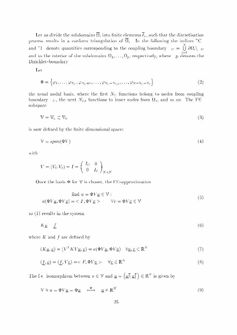
Let us divide the subdomains i into �nite elements �r, such that the discretisationprocess results in a conform triangulation of i. In the following the indices "C\and "I\ denote quantities corresponding to the coupling boundary �C = pSi=1 @in�Dand to the interior of the subdomains 1; : : : ;p, respectively, where �D denotes theDirichlet{boundary.Let� = n'1; : : : ; 'NC ; 'NC+1; : : : ; 'NC+NI;1 ; : : : ; 'N=NC+NIo (2)the usual nodal basis, where the �rst NC functions belong to nodes from couplingboundary �C , the next NI;1 functions to inner nodes from 1, and so on. The FE{subspaceV= Vh � V0 (3)is now de�ned by the �nite dimensional space:V= span(�V ) (4)with V = (VC VI) = I = IC 00 II !N�NOnce the basis � for V is chosen, the FE{approximation�nd u = �V u 2 V :a(�V u;�V v) =< F;�V v > 8v = �V v 2 V (5)to (1) results in the systemKu = f (6)where K and f are de�ned by(Ku; v) = (V TKV u; v) = a(�V u;�V v) 8u; v 2 RN (7)(f; v) = (f; V v) =< F;�V v > 8v 2 RN (8)The f.e. isomorphism between u 2 V and u = �uTC uTI � 2 RN is given byV3 u = �V u = �u � ! u 2 RN (9)25

Taking into account the arrangement of the basis function given in (2) we can rewritethe system (6) in the block form KC KCIKIC KI ! uCuI ! = fCf I ! (10)with KI = diag(KI;i)i=1;2;:::;p (11)The well known FE substructure technique gives a factorization of KK = IC KCIK�1IO II ! SC OO KI ! IC OK�1I KIC II !containing the Schur complement SC = KC �KCIK�1I KIC .In the next section we will apply a via Domain Decomposition parallized and pre-conditioned CG{method to system (10).2 A parallized CG{method for shared memory sys-temsThe method described here is derived from a parallel algorithm, developed for dis-tributed memory computers (see [HLM91]).The aim of this implementation was to make explicit use of shared memory forparallization. From this it seemed to be naturally to work with global data�elds andnot to split the matrices and vectors in local parts. The base to realize this was themultithreading programming model.The domain decomposition underlies the parallization as in the message passingcase, but contrary to this the coupling nodes (which are not splitted in local parts) areused by several processors, what causes problems for the parallization.A consequence is that every thread uses a part of the global matrix K and not thesuperelementmatrices Ki. For all components assigned to inner nodes this obviouslymakes no di�erence. For nodes assigned to the coupling boundary a unique assignmentto the threads needs to be found. For example the matrix K can be divided as follows�fKs�ij = 8>>><>>>: kij : !i; !j 2 s^�s = minr n!i 2 ro _ s = minr n!j 2 ro�0 : else (12)26

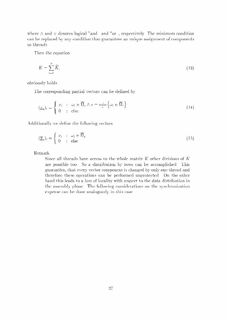
where ^ and _ denotes logical "and\ and "or\, respectively. The minimum conditioncan be replaced by any condition that guarantees an unique assignment of componentsto threads.Then the equationK = pXi=1 fKi (13)obviously holds.The corresponding partial vectors can be de�ned by(xs)i = 8<: xi : !i 2 s ^ s = minr n!i 2 ro0 : else (14)Additionally we de�ne the following vectors(xs)i = ( xi : !i 2 s0 : else (15)RemarkSince all threads have access to the whole matrix K other divisions of Kare possible too. So a distribution by rows can be accomplished. Thisguaranties, that every vector component is changed by only one thread andtherefore these operations can be performed unprotected. On the otherhand this leads to a loss of locality with respect to the data distribution inthe assembly phase. The following considerations on the synchronizationexpense can be done analogously in this case.27

With the notations above we can formulate the parallel algorithm:for i = 1; 2; : : : p do in parallel0. Start StepChoose an initial guess u, e.g. u = Ori = f iri = ri � fKiuiw = PC�1risi = wi�i = wTi ri� = �0 = P�iIteration1. evi = 0evi = evi + fKies�i = evTi esi� =P �i� = e�=�2. ui = eui + �esiri = eri � �evi3. w = PC�1ri4. �i = wTi ri� =P �i� = �=e�5. si = wi + �esi6. � � �2 � �0 ? no�! goto 1#yesstopIn the algorithm above the tilde symbol "e\ marks the old iterates.After steps 1 and 4 a global synchronization is necessary in order to make sure thatthe scalar products are completely evaluated. Additionally you need a synchronizationbetween step 5 an step 1. Here threads that have common nodes have to be synchro-nized, and this synchronization is really additional compared to the message passingalgorithm described in [HLM91]. Step 3 will be discussed in the next section. We onlynote here that in the case C = I this step results in the local operation wi = ri.2.1 The hierarchical DD-preconditioningIn the message passing algorithm described in [HLM91] a requirement is, that a precon-ditioner should not increase the communication amount signi�cantly. Various precon-ditioners satisfying this condition were presented in [HLM90, HLM91]. One example28

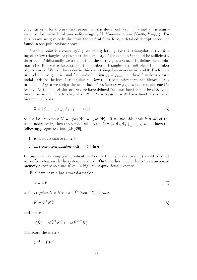
that was used for the practical experiments is described here. This method is equiv-alent to the hierarchical preconditioning by H. Yserentant (see [Yse86, Yse90]). Forthis reason we give only the basic theoretical facts here, a detailed decription can befound in the publications above.Starting point is a coarse grid (user triangulation). By this triangulation (consist-ing of as few triangles as possible) the geometry of the domain should be su�cientlydescribed. Additionally we assume that these triangles are used to de�ne the subdo-mains i. Hence it is favourable if the number of triangles is a multiple of the numberof processors. We call the nodes in this start triangulation nodes in level 0. Each nodein level 0 is assigned a usual f.e. basis function i = 'h0;i, i.e. these functions form anodal basis for the level 0 triangulation. Now the triangulation is re�ned hierarchicallyin l steps. Again we assign the usual basis functions i = 'hj ;i to nodes supervened inlevel j. At the end of this process we have de�ned N0 basis functions in level 0, N1 inlevel 1 an so on. The totality of all N = N0 + N1 + : : :+ Nl basis functions is calledhierarchical basis = f 1; : : : ; N0; N0+1; : : : ; Ng (16)of the f.e. subspace V = span() = span(�). If we use this basis instead of theusual nodal basis, then the associated matrix K̂ = (a(i;j))i;j=1;:::;N would have thefollowing properties: (see [Mey90])1. K̂ is not a sparse matrix2. The condition number �(K̂) = O(j ln hj2)Because of 2. the conjugate gradient method (without preconditioning) would be a fastsolver for sytems with the system matrix K̂. On the other hand 1. leads to an increasedmemory expense to store K̂ and a higher computational expense.But if we have a basis transformation = �V̂ (17)with a regular N �N -matrix V̂ from (17) follows:K̂ = V̂ TKV̂ (18)and hence�(K̂) = �(V̂ TKV̂ ) = �(V̂ V̂ TK)Therefore the matrixC�1 = V̂ V̂ T 29

is a good preconditioner for the System Ku = f in the nodal basis �.The matrix multiplicationw = V̂ V̂ T rcan be performed very e�ciently (only N multiplications and 2N additions are needed).We have to perform the multiplicationsy = V̂ T r and w = V̂ yThis is done by a factorisationV̂ = V̂ (l)V̂ (l�1) : : : V̂ (1) (19)(see [Yse86]). Now we de�ne matrices analogous to fKi:�V̂ (k)s �ij = 8>>><>>>: v(k)ij : !i; !j 2 s^�s = minr n!i 2 ro _ s = minr n!j 2 ro�0 : else (20)k = 1; 2; : : : ; lwherev(k)ij = �V̂ (k)�ijThen step 3 of the parallel algorithm described in section 2 leads toyi = 0; yi = yi + �V̂ (1)i �T : : : �V̂ (l�1)i �T �V̂ (l)i �T ri (21)wi = V̂ (l)i V̂ (l�1)i : : : V̂ (1)i yi (22)If we rewrite (21) in the formy(1)i = 0; y(1)i = y(1)i + �V̂ (l)i �T riy(k+1)i = y(k)i ; y(k+1)i = y(k+1)i + �V̂ (l�k)i �T y(k)i (k = 1; : : : ; l� 1)yi = y(l)iand (22) as followsw(1)i = V̂ (1)i yiw(k+1)i = V̂ (k+1)i w(k)i (k = 1; : : : ; l� 1)wi = w(l)iit is obvious that a synchronization is needed after each level, i.e. (2�l) synchronizationsare needed to perform the preconditioning.30

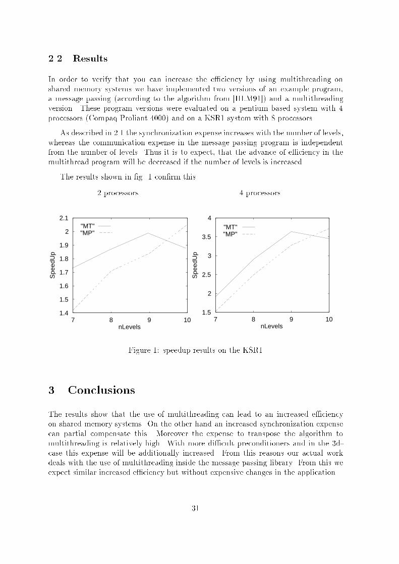
2.2 ResultsIn order to verify that you can increase the e�ciency by using multithreading onshared memory systems we have implemented two versions of an example program,a message passing (according to the algorithm from [HLM91]) and a multithreadingversion. These program versions were evaluated on a pentium based system with 4processors (Compaq Proliant 4000) and on a KSR1 system with 8 processors.As described in 2.1 the synchronization expense increases with the number of levels,whereas the communication expense in the message passing program is independentfrom the number of levels. Thus it is to expect, that the advance of e�ciency in themultithread program will be decreased if the number of levels is increased.The results shown in �g. 1 con�rm this.2 processors1.4

1.5

1.6

1.7

1.8

1.9

2

2.1

7 8 9 10

Spe

edU

p

nLevels

"MT""MP"

4 processors1.5

2

2.5

3

3.5

4

7 8 9 10

Spe

edU

p

nLevels

"MT""MP"

Figure 1: speedup results on the KSR13 ConclusionsThe results show that the use of multithreading can lead to an increased e�ciencyon shared memory systems. On the other hand an increased synchronization expensecan partial compensate this. Moreover the expense to transpose the algorithm tomultithreading is relatively high. With more di�cult preconditioners and in the 3d-case this expense will be additionally increased. From this reasons our actual workdeals with the use of multithreading inside the message passing library. From this weexpect similar increased e�ciency but without expensive changes in the application.31

References[HLM90] G. Haase, U. Langer, and A. Meyer, A new approach to the Dirichlet do-main decomposition method, Fifth Multigrid Seminar, Eberswalde, 1990(S. Hengst, ed.), Karl{Weierstrass{Institut, 1990, Report R{MATH{09/90,pp. 1{59.[HLM91] G. Haase, U. Langer, and A. Meyer, Parallelisierung und Vorkonditionierungdes CG-Verfahrens durch Gebietszerlegung, Proceedings of the GAMM-Seminar "Numerische Algorithmen auf Transputersystemen" held at Hei-delberg, 1991, Teubner Verlag, Stuttgart, 1991.[Mey90] A. Meyer, A parallel preconditioned conjugate gradient method using domaindecomposition and inexat solvers on each subdomain, Computing 45 (1990),217{234.[Yse86] H. Yserentant, On the multi{level splitting of �nite element spaces, Numer.Math. 49 (1986), no. 4, 379{412.[Yse90] H. Yserentant, Two preconditioners based on the multi{level splitting of �niteelement spaces, Numer. Math. 58 (1990), 163{184.

32

Leistungsvergleich ausgew�ahlter Funktionenverschiedener MPI-ImplementierungenJ�org Wernerjwern@informatik.tu-chemnitz.dehttp://noah.informatik.tu-chemnitz.de/members/werner/werner.html1 Leistungsvergleich ausgew�ahlter PARIX- undMPI-Kommunikationsfunktionen1.1 Aufbau des TestprogrammsDas Testprogramm wurde als MPI- und als PARIX-Version implentiert. Beide Versi-on nutzen das gleiche Rahmen-Programm und ein identisches Testfunktions-Interface.Alle Testroutinen stellen unabh�angig von der Implementierung die gleiche Funktiona-lit�at zur Verf�ugung. Das Programm umfa�t Leistungsmessungen f�ur Punkt-zu-Punkt-Kommunikation (blockierend, nichtblockierend), globale bzw. kollektive Kommunika-tion (Barrier, Broadcast, globale Reduktion) und topologiebezogene Kommunikation.Da PARIX keine Routinen f�ur globale Kommunikation bereitstellt, wurden diesemit den verf�ugbaren elementaren Sende- und Empfangsfunktionen nachgebildet.Art und Parameter des durchzuf�uhrenden Test werden dem Hauptprogramm alsParameter �ubergeben. Je Programmlauf kann f�ur einen spezi�schen Einzeltest eineMe�reihe erstellt werden. Eine Me�reihe umfa�t eine vom Nutzer bestimmbare Anzahlvon Einzelmessungen mit verschiedenen Datenpaketgr�o�en. Pro Einzelmessung wirddie f�ur den Test ben�otigte Zeit bei einer festen Datenpaketgr�o�e mit einer bestimmtenAnzahl Wiederholungen protokolliert.1.1.1 ZeitmessungIn der MPI-Version basiert die Zeitmessung auf MPI Wtime(). Diese Funktion liefert dieaktuelle Systemzeit in Form von Sekunden. In der PARIX-Version wurde die FunktionTimeNowLow() benutzt, welche die Systemzeit knotenlokal mit einer Au �osung von 64�s zur�uckgibt.Die Anzahl der Wiederholungen pro Einzeltest wurde im Allgemeinen so gew�ahlt,da� die akkumulierte Gesamtzeit im Sekundenbereich lag.1.1.2 Knotenident�kationSowohl PARIX als auch MPI bieten Routinen an, um die eigene Knotennummer alseindeutigen Identi�kator innerhalb der angeforderten Partition abzufragen. Die ermit-telten Knotennummern stimmen f�ur PARIX und MPI �uberein. Diese Pr�ufung warinsofern notwendig, da einige der Tests eindeutig festlegte Kommunikationspaare er-fordern. 33

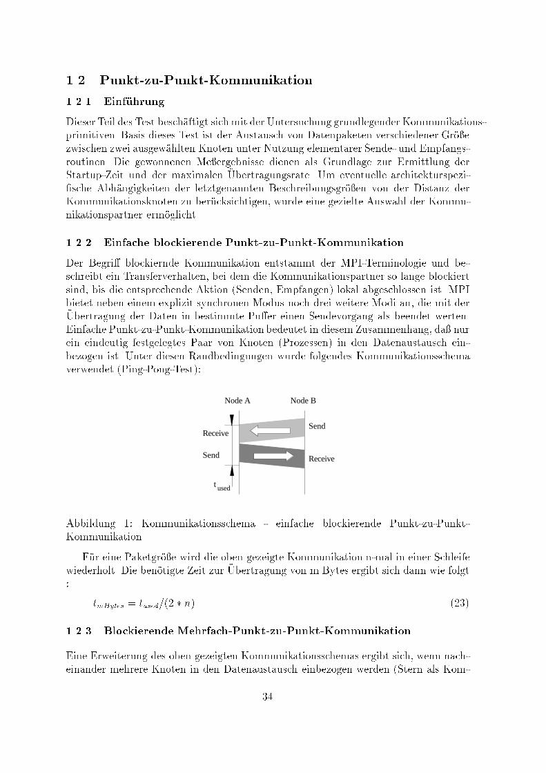
1.2 Punkt-zu-Punkt-Kommunikation1.2.1 Einf�uhrungDieser Teil des Test besch�aftigt sich mit der Untersuchung grundlegender Kommunikations-primitiven. Basis dieses Test ist der Austausch von Datenpaketen verschiedener Gr�o�ezwischen zwei ausgew�ahlten Knoten unter Nutzung elementarer Sende- und Empfangs-routinen. Die gewonnenen Me�ergebnisse dienen als Grundlage zur Ermittlung derStartup-Zeit und der maximalen �Ubertragungsrate. Um eventuelle architekturspezi-�sche Abh�angigkeiten der letztgenannten Beschreibungsgr�o�en von der Distanz derKommunikationsknoten zu ber�ucksichtigen, wurde eine gezielte Auswahl der Kommu-nikationspartner erm�oglicht.1.2.2 Einfache blockierende Punkt-zu-Punkt-KommunikationDer Begri� blockiernde Kommunikation entstammt der MPI-Terminologie und be-schreibt ein Transferverhalten, bei dem die Kommunikationspartner so lange blockiertsind, bis die entsprechende Aktion (Senden, Empfangen) lokal abgeschlossen ist. MPIbietet neben einem explizit synchronen Modus noch drei weitere Modi an, die mit der�Ubertragung der Daten in bestimmte Pu�er einen Sendevorgang als beendet werten.Einfache Punkt-zu-Punkt-Kommunikation bedeutet in diesemZusammenhang, da� nurein eindeutig festgelegtes Paar von Knoten (Prozessen) in den Datenaustausch ein-bezogen ist. Unter diesen Randbedingungen wurde folgendes Kommunikationsschemaverwendet (Ping-Pong-Test):Node A Node B

SendReceive

ReceiveSend

t usedAbbildung 1: Kommunikationsschema - einfache blockierende Punkt-zu-Punkt-KommunikationF�ur eine Paketgr�o�e wird die oben gezeigte Kommunikation n-mal in einer Schleifewiederholt. Die ben�otigte Zeit zur �Ubertragung von m Bytes ergibt sich dann wie folgt: tmBytes = tused=(2 � n) (23)1.2.3 Blockierende Mehrfach-Punkt-zu-Punkt-KommunikationEine Erweiterung des oben gezeigten Kommunikationsschemas ergibt sich, wenn nach-einander mehrere Knoten in den Datenaustausch einbezogen werden (Stern als Kom-34

munikationsger�ust). Dadurch lassen sich zus�atzliche Aussagen ableiten.F�ur echte synchrone Kommunikation besitzen die Resulte zur Transferdauer einenallgemeineneren Charakter, da in diesem Fall nicht nur eine (gegebenenfalls minimale)Distanz bewertet wird, sondern mehrere verschiedene. Der so ermittelte Wert k�onnteals mittlere Kommunikationsdauer f�ur eine bestimme Paketgr�o�e bezeichnet werden.Parallelrechner, deren Startup-Zeit und Kommunikationsbandbreite abh�angig sind vonder Distanz der einbezogenen Knoten, werden bei dieser Messung Resultate aufweisen,die sich von den Werten einer einzelnen und eindeutigen Punkt-zu-Punkt-Verbindungunterscheiden.Bei Verwendung pu�ernder MPI-Modi (Standard, Ready, Bu�ered) besteht dieM�oglichkeit der teilweisen �Uberlagerung des Datenaustausches. Mit der R�uckkehr vonder Senderoutine kann so bereits vom n�achsten Knoten empfangen werden, obwohl derletzte Sendevorgang physisch noch nicht beendet wurde (siehe Abb. 2).Node A Node B

SendReceive

ReceiveSend

t used

Node N

Send

Receive

Receive

SendAbbildung 2: Kommunikationsschema - blockierende Mehrfach -Punkt-zu-Punkt-KommunikationF�ur eine Paketgr�o�e wird die oben gezeigte Kommunikation n-mal in einer Schleifewiederholt. Die ben�otigte Zeit zur �Ubertragung von m Bytes unter Beteiligung von kKnoten (1 Master(Node A), k-1 Slaves(Node B bis Node N)ergibt sich dann wie folgt :tmBytes = tused=(2 � n � k � 1) (24)1.2.4 Nichtblockierende Punkt-zu-Punkt-KommunikationDie Anwendung nichtblockierenderKommunikationsroutinen erm�oglichtAussagen dar�uber,wie e�ektiv sich verschiedene Kommunikationsanforderungen �uberlagern lassen bzw.wie gro� ein damit verbundener zus�atzlicher Overhead ist. Alle nichtblockierendenKommunikationsroutinen erfordern den separaten Aufruf von Funktionen, die die Be-endigung einer Daten�ubertragung testen bzw. auf diese warten (sogenannte Complete-Rufe). Analog zum vorangegangenen Abschnitt erstrecken sich die Untersuchungen auf35

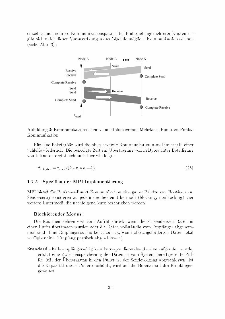
einzelne und mehrere Kommunikationspaare. Bei Einbeziehung mehrerer Knoten er-gibt sich unter diesen Voraussetzungen das folgende m�ogliche Kommunikationsschema(siehe Abb. 3) :Node A Node B

SendReceive

ReceiveSend

t used

Node N

Send

Receive

Receive

Send

Complete Send

Complete Receive

Complete Send

Complete ReceiveAbbildung 3: Kommunikationsschema - nichtblockierende Mehrfach -Punkt-zu-Punkt-KommunikationF�ur eine Paketgr�o�e wird die oben gezeigte Kommunikation n-mal innerhalb einerSchleife wiederholt. Die ben�otigte Zeit zur �Ubertragung von m Bytes unter Beteiligungvon k Knoten ergibt sich auch hier wie folgt :tmBytes = tused=(2 � n � k � 1) (25)1.2.5 Spezi�ka der MPI-ImplementierungMPI bietet f�ur Punkt-zu-Punkt-Kommunikation eine ganze Palette von Routinen an.Senderseitig existieren zu jedem der beiden �Ubermodi (blocking, nonblocking) vierweitere Untermodi, die nachfolgend kurz beschrieben werden.Blockierender Modus :Die Routinen kehren erst vom Aufruf zur�uck, wenn die zu sendenden Daten ineinen Pu�er �ubertragen wurden oder die Daten vollst�andig vom Empf�anger abgenom-men sind. Eine Empfangsroutine kehrt zur�uck, wenn alle angeforderten Daten lokalverf�ugbar sind (Empfang physisch abgeschlossen).Standard - Falls empf�angerseitig kein korrespondierendes Receive aufgerufen wurde,erfolgt eine Zwischenspeicherung der Daten in vom System bereitgestellte Puf-fer. Mit der �Ubertragung in den Pu�er ist der Sendevorgang abgeschlossen. Istdie Kapazit�at dieser Pu�er ersch�opft, wird auf die Bereitschaft des Empf�angersgewartet. 36

Bu�ered - Die Daten werden in einen vom Nutzer bereitzustellenden Pu�er �ubertra-gen. Die Sendeoperation kehrt nach der Zwischenpu�erung unverz�uglich zur�uck.Unterdimensionierter Pu�er f�uhren zu einem Fehler und nicht zum Warten aufEmpfangsbereitschaft.Synchron - Es wird solange gewartet, bis eine korrespondierende Empfangsroutinegerufen wurde. Die Daten�ubertragung erfolgt ohne Zwischenspeicherung direktin den vom Empf�anger angegebenen Datenbereich.Ready - Das MPI-Forum hat diesen Modus so de�niert, da� ein Ready-Send un-verz�uglich zur�uckkehrt, wenn das passende Receive nicht bereits aktiv ist. Diemeisten Implementierungen setzen diesen Modus aufgrund der schlechten Hand-habbarkeit mit dem Standard-Mode gleich.Nichtblockierender Modus :Mit dem Ruf der entsprechenden Routine werden nur noch Sende- bzw. Empfangs-anforderungen (Requests) gestellt. Nach Abgabe des Requests kehren die Routinenunverz�uglich zur�uck. Mit Hilfe von Statusabfragen l�a�t sich der Zustand einer laufen-den Kommunikation ermitteln oder auf dessen Ende warten. Auch hier stehen die vieroben genannten Modi mit den dort erl�auterten Spezi�ka zur Verf�ugung.Empfangsseitig beschr�ankt sich die Anzahl der zur Verf�ugung stehenden Routinenauf eine blockierende und eine nichtblockierende Funktion. Es sind beliebige Kombi-nationen zwischen den 8 Sende- und 2 Empfangsroutinen zul�assig. Ein blockierendessynchrones Send darf demnach von einem nichtblockierenden Receive bedient werden.Auf diese M�oglichkeit wurde innerhalb des Testprogrammes verzichtet. Somit stehenf�ur die Punkt-zu-Punkt-Kommunikation acht Modi zur Verf�ugung (4 blockierende, 4nichtblockierende).1.2.6 Spezi�ka der Parix-ImplementierungPARIX bietet f�ur synchrone linkgebundene Punkt-zu-Punkt-Kommunikation lediglicheine Empfangs- und eine Senderoutine an. In PARIX-Terminologie bedeutet synchron,da� eine erfolgreiche Kommunikation unbedingt die Bereitschaft beider Partner erfor-dert. Eine Verletzung dieser Bedingung f�uhrt zu einem Deadlock.Im Unterschied zu MPI sind in PARIX die bidirektionalen Kommunikationskan�ale(Links) vor der ersten Benutzung explizit zu er�o�nen. Nach der Er�o�nung einer Link istdie weitere Handhabung w�ahrend des Datenaustausches weitgehend identisch zu MPI.Unterschiede ergeben sich nur im Adressierungsschema. PARIX verwendet zur Be-stimmung des Kommunikationspartners den Namen der dorthin errichteten Link, MPIbenutzt zur Adressierung ein Knotennummer-Kommunikationskontext-Paar (Rank-Communicator).Asynchrone Kommunikation (gleichbedeutend mit nichtblockierend in MPI) l�a�t37

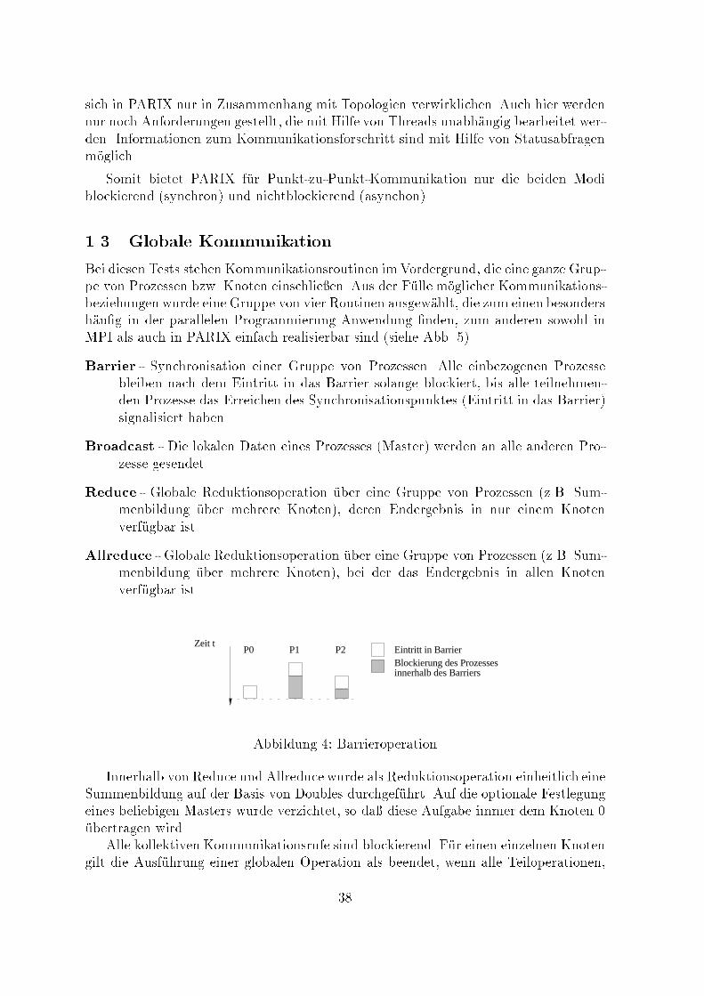
sich in PARIX nur in Zusammenhang mit Topologien verwirklichen. Auch hier werdennur noch Anforderungen gestellt, die mit Hilfe von Threads unabh�angig bearbeitet wer-den. Informationen zum Kommunikationsforschritt sind mit Hilfe von Statusabfragenm�oglich.Somit bietet PARIX f�ur Punkt-zu-Punkt-Kommunikation nur die beiden Modiblockierend (synchron) und nichtblockierend (asynchon).1.3 Globale KommunikationBei diesen Tests stehen Kommunikationsroutinen imVordergrund, die eine ganze Grup-pe von Prozessen bzw. Knoten einschlie�en. Aus der F�ulle m�oglicher Kommunikations-beziehungen wurde eine Gruppe von vier Routinen ausgew�ahlt, die zum einen besondersh�au�g in der parallelen Programmierung Anwendung �nden, zum anderen sowohl inMPI als auch in PARIX einfach realisierbar sind (siehe Abb. 5).Barrier - Synchronisation einer Gruppe von Prozessen. Alle einbezogenen Prozessebleiben nach dem Eintritt in das Barrier solange blockiert, bis alle teilnehmen-den Prozesse das Erreichen des Synchronisationspunktes (Eintritt in das Barrier)signalisiert haben.Broadcast - Die lokalen Daten eines Prozesses (Master) werden an alle anderen Pro-zesse gesendet.Reduce - Globale Reduktionsoperation �uber eine Gruppe von Prozessen (z.B. Sum-menbildung �uber mehrere Knoten), deren Endergebnis in nur einem Knotenverf�ugbar ist.Allreduce - Globale Reduktionsoperation �uber eine Gruppe von Prozessen (z.B. Sum-menbildung �uber mehrere Knoten), bei der das Endergebnis in allen Knotenverf�ugbar ist.Eintritt in BarrierBlockierung des Prozessesinnerhalb des Barriers

Zeit tP0 P1 P2Abbildung 4: BarrieroperationInnerhalb von Reduce und Allreduce wurde als Reduktionsoperation einheitlich eineSummenbildung auf der Basis von Doubles durchgef�uhrt. Auf die optionale Festlegungeines beliebigen Masters wurde verzichtet, so da� diese Aufgabe immer dem Knoten 0�ubertragen wird.Alle kollektiven Kommunikationsrufe sind blockierend. F�ur einen einzelnen Knotengilt die Ausf�uhrung einer globalen Operation als beendet, wenn alle Teiloperationen,38

0

1 2 0

Prozeß bzw. n Knoten n

0

0

1 2 0

0

1

1

2

2

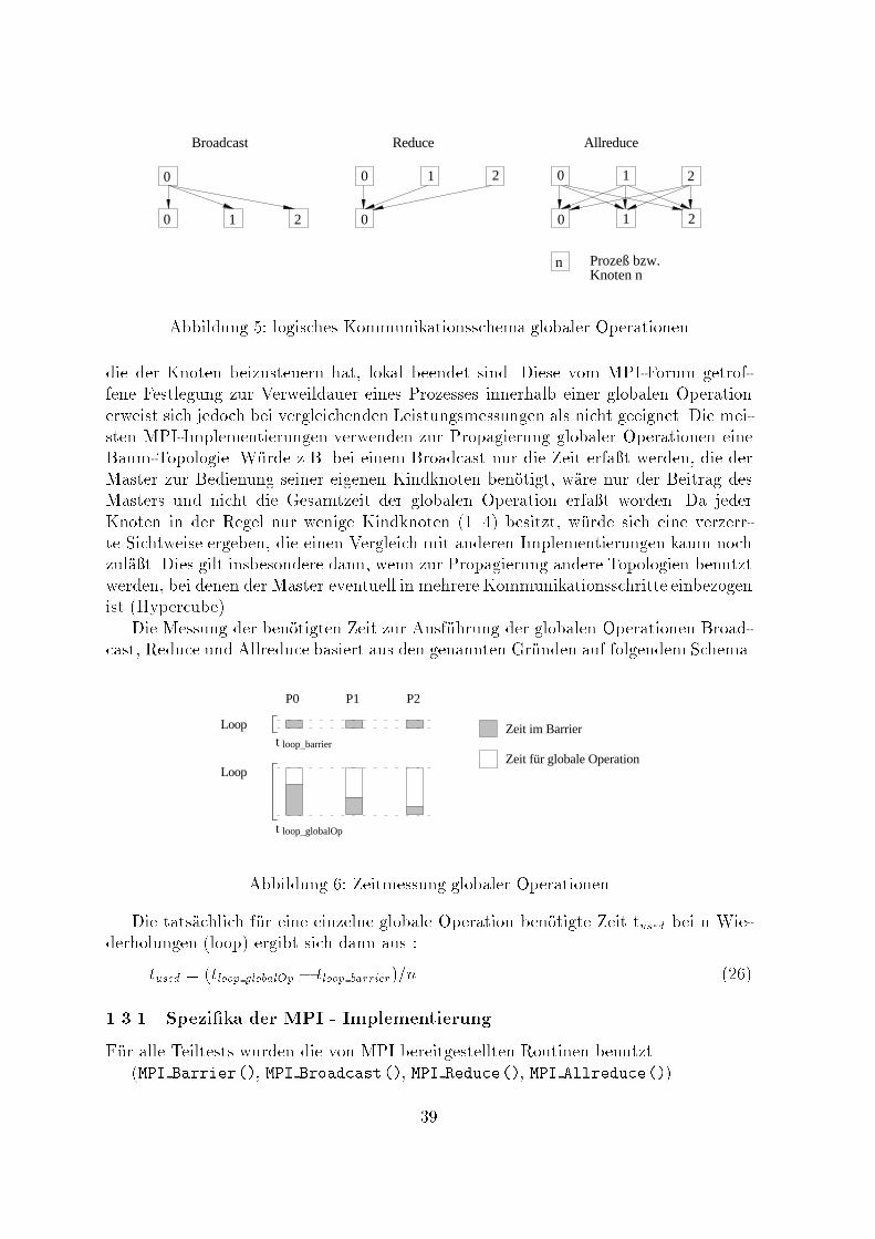
Broadcast Reduce Allreduce

Abbildung 5: logisches Kommunikationsschema globaler Operationendie der Knoten beizusteuern hat, lokal beendet sind. Diese vom MPI-Forum getrof-fene Festlegung zur Verweildauer eines Prozesses innerhalb einer globalen Operationerweist sich jedoch bei vergleichenden Leistungsmessungen als nicht geeignet. Die mei-sten MPI-Implementierungen verwenden zur Propagierung globaler Operationen eineBaum-Topologie. W�urde z.B. bei einem Broadcast nur die Zeit erfa�t werden, die derMaster zur Bedienung seiner eigenen Kindknoten ben�otigt, w�are nur der Beitrag desMasters und nicht die Gesamtzeit der globalen Operation erfa�t worden. Da jederKnoten in der Regel nur wenige Kindknoten (1..4) besitzt, w�urde sich eine verzerr-te Sichtweise ergeben, die einen Vergleich mit anderen Implementierungen kaum nochzul�a�t. Dies gilt insbesondere dann, wenn zur Propagierung andere Topologien benutztwerden, bei denen der Master eventuell in mehrere Kommunikationsschritte einbezogenist (Hypercube).Die Messung der ben�otigten Zeit zur Ausf�uhrung der globalen Operationen Broad-cast, Reduce und Allreduce basiert aus den genannten Gr�unden auf folgendem Schema.Zeit im Barrier

P0 P1 P2

Loop

Loop

t loop_barrier

t loop_globalOp

Zeit für globale OperationAbbildung 6: Zeitmessung globaler OperationenDie tats�achlich f�ur eine einzelne globale Operation ben�otigte Zeit tused bei n Wie-derholungen (loop) ergibt sich dann aus :tused = (tloop globalOp � tloop barrier)=n (26)1.3.1 Spezi�ka der MPI - ImplementierungF�ur alle Teiltests wurden die von MPI bereitgestellten Routinen benutzt.(MPI Barrier(), MPI Broadcast(), MPI Reduce(), MPI Allreduce())39

1.3.2 Spezi�ka der PARIX-ImplementierungPARIX bietet keinerlei vorde�nierte Bibliotheksfunktionen f�ur kollektive Kommunika-tion. Ben�otigt man als Anwender Operationen auf Gruppenniveau, ist die entsprechen-de Funktionalit�at mit Hilfe von Punkt-zu-Punkt-Kommunikation nachzubilden. DieE�zienz bzw. Leistungsf�ahigkeit solch kollektiver Routinen ist dabei vorrangig von derverwendeten Kommunikationstopologie abh�angig. Dabei sollte die ben�otigte Zeit zumVerteilen bzw. Sammeln von Daten nicht (idealerweise) oder nur in m�oglichst geringenMa�e von der Anzahl der beteiligten Knoten abh�angen. Das Idealziel der Entkopplungvon Leistungsf�ahigkeit und Prozessorzahl l�a�t sich oft nur �uber zus�atzliche Spezial-hardware l�osen und wurde nur ein wenigen Architekturen realisiert (Cray T3D).In der PARIX-Implementierung wurde die Funktionalit�at von Barrier, Broadcast,Reduce und Allreduce auf der Basis topologie- und linkgebundener Kommunikations-routinen (Send(), Recv()) verwirklicht. F�ur jeden der genannten Teiltests l�a�t sichdie zugrundeliegende Topologie aus einer der folgenden Alternativen ausw�ahlen :Stern-Topologie : Der Master besitzt zu jedem einbezogenen Knoten eine separateLink. Die teilnehmendenKnoten werden nacheinander bedient. F�ur die Bedienungvon n Prozessoren werden somit n Zeitschritte ben�otigt. Da dieses Vorgehen kei-nerlei Kommunkationsparallelit�at erm�oglicht, ist diese Topologie die une�ektivsteund am schlechtesten sklarierungsf�ahigste.Hypercube-Topologie : Diese Topologie l�a�t sich nur f�ur Prozessorzahlen n = 2k(k = 1..m) errichten. K wird als Dimension des Cubes bezeichnet. Die Anzahlben�otigter Kommunikationsschritte ist mit der Dimension identisch. In einemZeitschritt laufen 2k�1 Kommunikationen zueinander parallel ab.Baum-Topologie : Die Knoten bilden einen unbalancierter Baum. Jeder Knoten kannmaximal einen Elternknoten und n Kindknoten besitzen. Zur Durchf�uhrung einerBroadcast-Operation sind z.B. folgende Schritte Knoten-lokal auszuf�uhren.1) Wenn es einen Elternknoten gibt, empfange Daten von diesem Knoten.2) Leite die Daten an alle eigenen Kindknoten weiterAbbildung 7 zeigt die Reihenfolge der Kommunikationsschritte in einen unbalan-cierten Baum mit 8 Knoten.1.4 TopologienIm Unterschied zum vorangegangenen Abschnitt dienen Topologien hier nicht als in-ternes Mittel zum Erzielen einer gew�unschten Funktionalit�at. In diesem Abschnitt sindTopologien als eine dem Nutzer o�enstehende Methode zu sehen, Kommunikation aufeiner systematischeren Ebene durchzuf�uhren. F�ur einen Ring besteht diese abstraktereSicht darin, Kommunikationspartner nicht mehr konkret durch ihre Prozessornummerzu adressieren, sondern allgemeiner als linken und rechten Nachbarn anzusprechen. Einweiterer wichtiger Vorteil bei der Benutzung von Topologien liegt in der systematischenIntegrationsf�ahigkeit von Nutzerkenntnissen zum physisch vorhandenen Kommunikati-40

1

2

3

2

3

3

3

1

2

2

3 1

1

1Abbildung 7: Unbalancierter Baum f�ur 8 Knotenonsnetzwerk. Diese M�oglichkeit ist besonders bei Distributed Memory Parallelrechnermit dedizierten Kommunikationsnetzwerk und distanzabh�angigen Kommunikationspa-rametern wertvoll. Ein optimales Mapping der benutzten Softwarekan�ale auf die realenHardwareverbindungen wird bei Maschinen der obengenannten Architektur in der Re-gel zu einer besseren Performance f�uhren.Sowohl PARIX als auch MPI bieten diese M�oglichkeit, nutzerspezi�sche Topologienaufzubauen und zu nutzen. F�ur beide Versionen wurden die zwei folgenden topologie-bezogene Tests implementiert:Optimaler Ring : �Uber alle verf�ugbaren Knoten wird eine optimale Ringtopologieaufgebaut. Jeder Knoten kommuniziert dabei nur mit unmittelbar physisch be-nachbarten Knoten ( Distanz = konstant 1 Hops). Die Informationen zur ange-forderten Partition werden vom Laufzeitsystem abgefragt (Root-Struktur).Einfacher Ring : Der Aufbau einer einfachenRingtopologie erfolgt ohne weitere Ber�uck-sichtung von Randinformationen als reine Aneinanderreihung der Prozessornum-mern (bei n Prozessoren -> 0, 1, 2, ... , n-1, 0).8 9 10 11

4 5 6 7

0 1 2 3

8 9 10 11

4 5 6 7

0 1 2 3

Optimaler Ring Nichtoptimaler Ring

Abbildung 8: Kommunikationsschema - optimaler und einfacher RingDie Gegen�uberstellung beider Topologogietests erlaubt R�uckschl�usse, wie gut sichein optimales Mapping in der Praxis auswirkt. Gemessen wird jeweils die ben�otigte41

Zeit f�ur einen vollst�andigen Ringumlauf bei einer bestimmten Datenpaketgr�o�e.1.4.1 Spezi�ka der MPI-ImplementierungMPI bietet f�ur den topologiebezogenen Datenaustausch keine speziellen Kommunikati-onsfunktionen an. Es stehen alle unter Punkt-zu-Punkt-Kommunikation vorgestelltenRoutinen zur Verf�ugung. Die topologierelevanten Informationen sind dabei an einenKommunikationskontext (Communicator) gekoppelt. Alle Topologiedaten werden vomNutzer durch den Aufbau eines neuen Communicators integriert und k�onnen von denKnoten abgefragt werden. Jeder Knoten kann auf diese Weise ermitteln, wieviel Nach-barn er innerhalb der Topologie besitzt und welche Identi�katoren (Ranks) diese Kno-ten besitzen. Der Partner wird beim sp�ateren Datenaustausch durch Communicatorund Rank adressiert. Benutzt man das von MPI ermittelte Array der Nachbarn inZusammenhang mit einem (Richtungs-) Index, ergibt sich eine PARIX-�ahnliche Hand-habung.1.4.2 Spezi�ka der PARIX-ImplementierungDie Handhabung und Benutzung von Topologien ist in PARIX fest integriert. F�urdie synchrone Kommunikation auf Topologien existieren separate Befehle (Send(),Recv()). W�ahrend der Errichtung einer Topologie werden die er�o�neten Kan�ale ineiner internen Struktur gespeichert, auf die der Nutzer �uber einen Kanalindex Zugri�besitzt. Die Adressierung eines Kommunikationspartners erfolgt �uber die Spezi�zierungvon Topologie und Kanalindex.

42

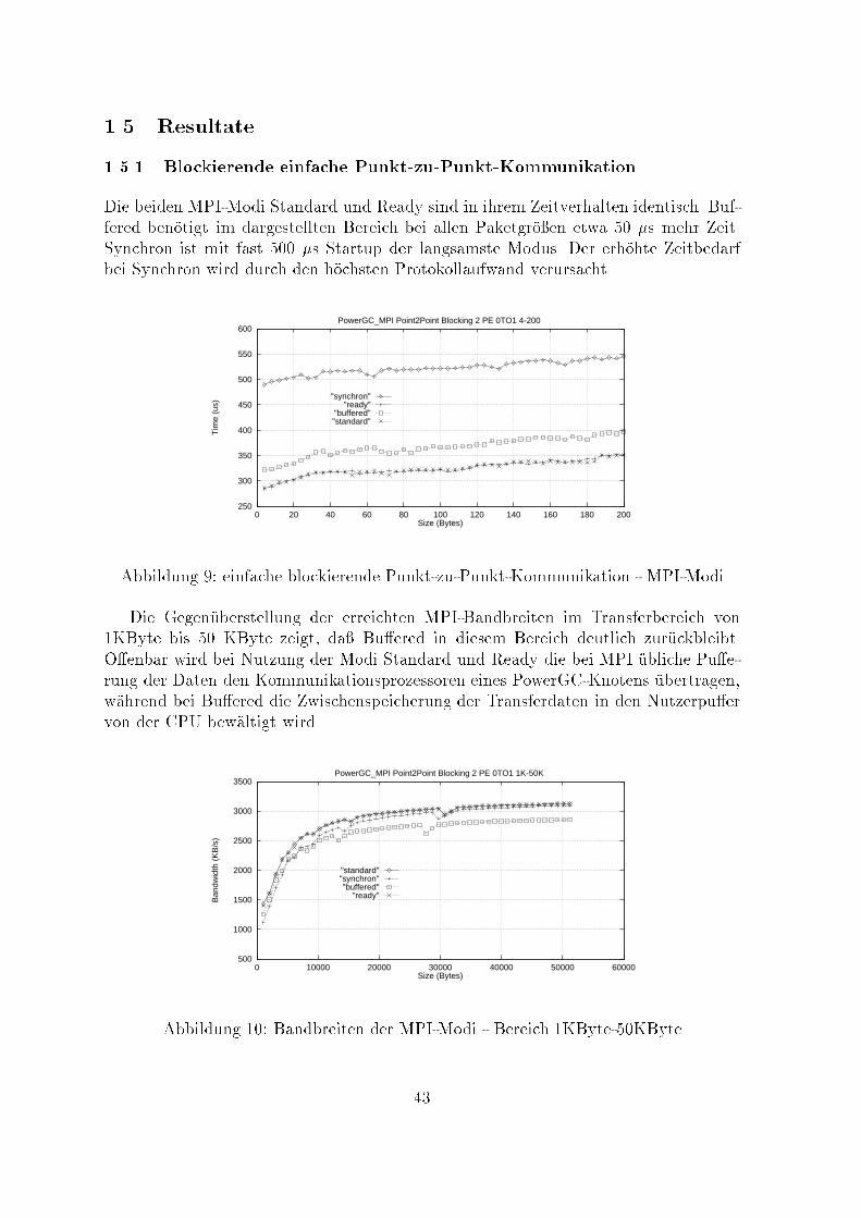
1.5 Resultate1.5.1 Blockierende einfache Punkt-zu-Punkt-KommunikationDie beiden MPI-Modi Standard und Ready sind in ihrem Zeitverhalten identisch. Buf-fered ben�otigt im dargestellten Bereich bei allen Paketgr�o�en etwa 50 �s mehr Zeit.Synchron ist mit fast 500 �s Startup der langsamste Modus. Der erh�ohte Zeitbedarfbei Synchron wird durch den h�ochsten Protokollaufwand verursacht.250

300

350

400

450

500

550

600

0 20 40 60 80 100 120 140 160 180 200

Tim

e (u

s)

Size (Bytes)

PowerGC_MPI Point2Point Blocking 2 PE 0TO1 4-200

"synchron""ready"

"buffered""standard"Abbildung 9: einfache blockierende Punkt-zu-Punkt-Kommunikation - MPI-ModiDie Gegen�uberstellung der erreichten MPI-Bandbreiten im Transferbereich von1KByte bis 50 KByte zeigt, da� Bu�ered in diesem Bereich deutlich zur�uckbleibt.O�enbar wird bei Nutzung der Modi Standard und Ready die bei MPI �ubliche Pu�e-rung der Daten den Kommunikationsprozessoren eines PowerGC-Knotens �ubertragen,w�ahrend bei Bu�ered die Zwischenspeicherung der Transferdaten in den Nutzerpu�ervon der CPU bew�altigt wird.

500

1000

1500

2000

2500

3000

3500

0 10000 20000 30000 40000 50000 60000

Ban

dwid

th (

KB

/s)

Size (Bytes)

PowerGC_MPI Point2Point Blocking 2 PE 0TO1 1K-50K

"standard""synchron""buffered"

"ready"Abbildung 10: Bandbreiten der MPI-Modi - Bereich 1KByte-50KByte43

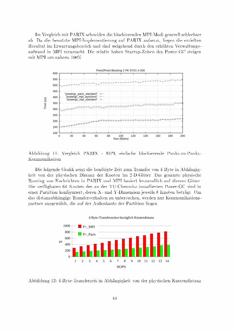
Im Vergleich mit PARIX schneiden die blockierenden MPI-Modi generell schlechterab. Da die benutzte MPI-Implementierung auf PARIX aufsetzt, liegen die erzieltenResultat im Erwartungsbereich und sind weigehend durch den erh�ohten Verwaltungs-aufwand in MPI verursacht. Die relativ hohen Startup-Zeiten des Power-GC steigenmit MPI um nahezu 100%.100

150

200

250

300

350

400

450

500

550

600

0 20 40 60 80 100 120 140 160 180 200

Tim

e (u

s)

Size (Bytes)

Point2Point Blocking 2 PE 0TO1 4-200

"powergc_parix_standard""powergc_mpi_synchron""powergc_mpi_standard"

Abbildung 11: Vergleich PARIX - MPI, einfache blockierende Punkt-zu-Punkt-KommunikationDie folgende Gra�k zeigt die ben�otigte Zeit zum Transfer von 4 Byte in Abh�angig-keit von der physischen Distanz der Knoten im 2-D-Gitter. Das gesamte physischeRouting von Nachrichten in PARIX und MPI basiert letztendlich auf diesem Gitter.Die verf�ugbaren 64 Knoten des an der TU-Chemnitz installierten Power-GC sind ineiner Partition kon�guriert, deren X- und Y-Dimension jeweils 8 Knoten betr�agt. Umdas distanzabh�angige Transferverhalten zu untersuchen, werden nur Kommunikations-partner ausgew�ahlt, die auf der Au�enkante der Partition liegen.4 Byte-Transferzeiten bezüglich Knotendistanz

HOPS

µs

0

200

400

600

800

1000

1 2 3 4 5 6 7 8 9 10 11 12 13 14

P+_MPI

P+_ParixAbbildung 12: 4-Byte-Transferzeit in Abh�angigkeit von der physischen Knotendistanz44

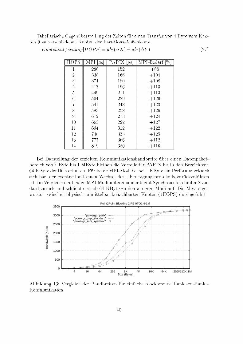
Tabellarische Gegen�uberstellung der Zeiten f�ur einen Transfer von 4 Byte vom Kno-ten 0 zu verschiedenen Knoten der Partitions-Au�enkante.Knotenentfernung[HOPS] = abs(�X) + abs(�Y ) (27)HOPS MPI [�s] PARIX [�s] MPI-Bedarf [%]1 286 152 +882 338 166 +1043 374 180 +1084 417 196 +1135 449 211 +1136 504 229 +1207 541 243 +1238 583 258 +1269 612 273 +12410 663 292 +12711 694 312 +12212 748 333 +12513 777 366 +11214 819 380 +116Bei Darstellung der erzielten Kommunikationsbandbreite �uber einen Datenpaket-bereich von 4 Byte bis 1 MByte bleiben die Vorteile f�ur PARIX bis in den Bereich von64 KByte deutlich erhalten. F�ur beide MPI-Modi ist bei 1 KByte ein Performanceknicksichtbar, der eventuell auf einen Wechsel des �Ubertragungsprotokolls zur�uckzuf�uhrenist. Im Vergleich der beiden MPI-Modi untereinander bleibt Synchron stets hinter Stan-dard zur�uck und schlie�t erst ab 64 KByte zu den anderen Modi auf. Die Messungenwurden zwischen physisch unmittelbar benachbarten Knoten (1HOPS) durchgef�uhrt.0

500

1000

1500

2000

2500

3000

3500

4 16 64 256 1K 4K 16K 64K 256K512K 1M

Ban

dwid

th (

KB

/s)

Size (Bytes)

Point2Point Blocking 2 PE 0TO1 4-1M

"powergc_parix""powergc_mpi_standard""powergc_mpi_synchron"

Abbildung 13: Vergleich der Bandbreiten f�ur einfache blockierende Punkt-zu-Punkt-Kommunikation 45

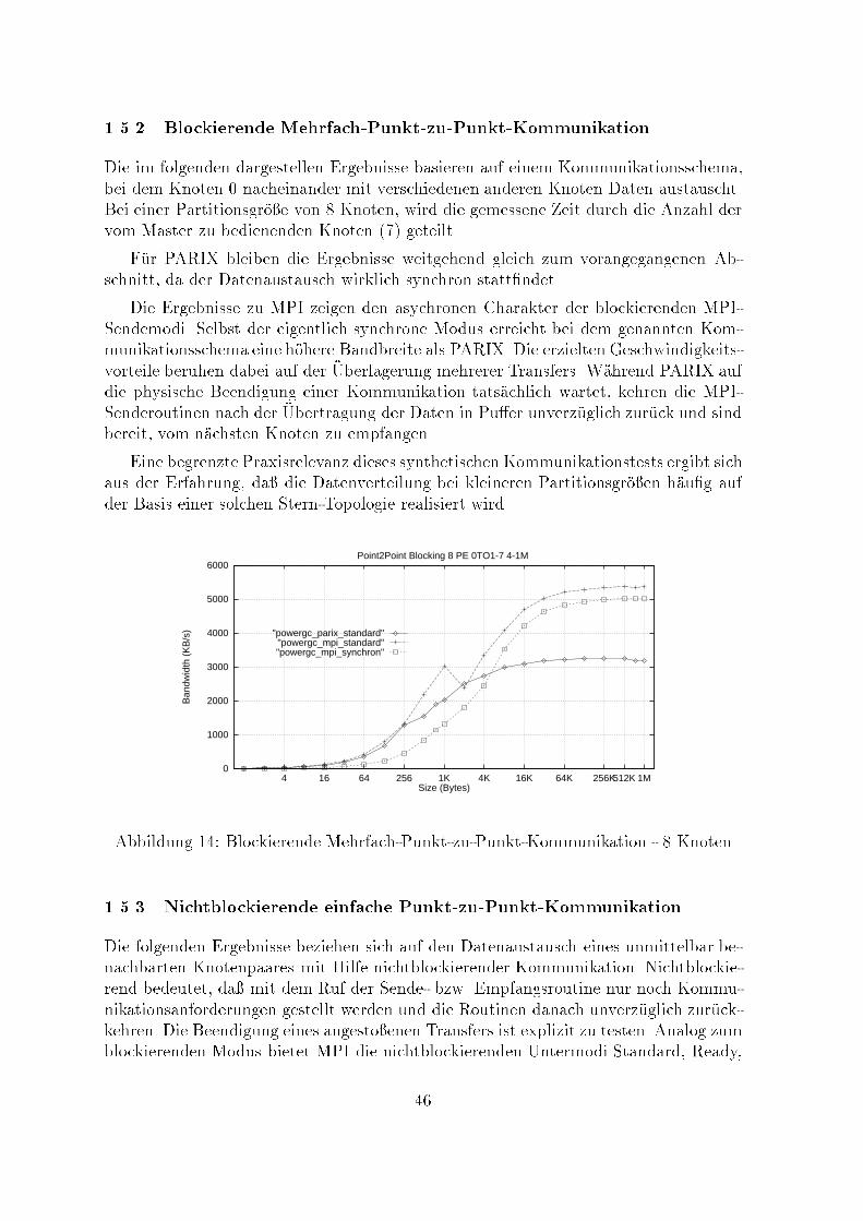
1.5.2 Blockierende Mehrfach-Punkt-zu-Punkt-KommunikationDie im folgenden dargestellen Ergebnisse basieren auf einem Kommunikationsschema,bei dem Knoten 0 nacheinander mit verschiedenen anderen Knoten Daten austauscht.Bei einer Partitionsgr�o�e von 8 Knoten, wird die gemessene Zeit durch die Anzahl dervom Master zu bedienenden Knoten (7) geteilt.F�ur PARIX bleiben die Ergebnisse weitgehend gleich zum vorangegangenen Ab-schnitt, da der Datenaustausch wirklich synchron statt�ndet.Die Ergebnisse zu MPI zeigen den asychronen Charakter der blockierenden MPI-Sendemodi. Selbst der eigentlich synchrone Modus erreicht bei dem genannten Kom-munikationsschema eine h�ohere Bandbreite als PARIX. Die erzielten Geschwindigkeits-vorteile beruhen dabei auf der �Uberlagerung mehrerer Transfers. W�ahrend PARIX aufdie physische Beendigung einer Kommunikation tats�achlich wartet, kehren die MPI-Senderoutinen nach der �Ubertragung der Daten in Pu�er unverz�uglich zur�uck und sindbereit, vom n�achsten Knoten zu empfangen.Eine begrenzte Praxisrelevanz dieses synthetischen Kommunikationstests ergibt sichaus der Erfahrung, da� die Datenverteilung bei kleineren Partitionsgr�o�en h�au�g aufder Basis einer solchen Stern-Topologie realisiert wird.0

1000

2000

3000

4000

5000

6000

4 16 64 256 1K 4K 16K 64K 256K512K 1M

Ban

dwid

th (

KB

/s)

Size (Bytes)

Point2Point Blocking 8 PE 0TO1-7 4-1M

"powergc_parix_standard""powergc_mpi_standard""powergc_mpi_synchron"

Abbildung 14: Blockierende Mehrfach-Punkt-zu-Punkt-Kommunikation - 8 Knoten1.5.3 Nichtblockierende einfache Punkt-zu-Punkt-KommunikationDie folgenden Ergebnisse beziehen sich auf den Datenaustausch eines unmittelbar be-nachbarten Knotenpaares mit Hilfe nichtblockierender Kommunikation. Nichtblockie-rend bedeutet, da� mit dem Ruf der Sende- bzw. Empfangsroutine nur noch Kommu-nikationsanforderungen gestellt werden und die Routinen danach unverz�uglich zur�uck-kehren. Die Beendigung eines angesto�enen Transfers ist explizit zu testen. Analog zumblockierenden Modus bietet MPI die nichtblockierenden Untermodi Standard, Ready,46

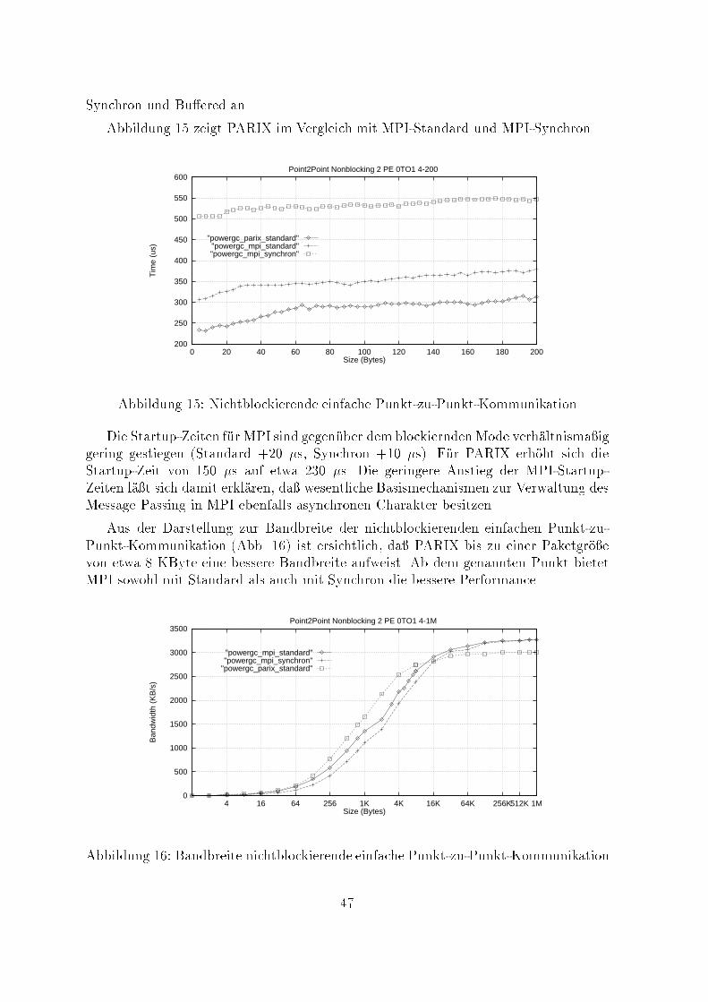
Synchron und Bu�ered an.Abbildung 15 zeigt PARIX im Vergleich mit MPI-Standard und MPI-Synchron.200

250

300

350

400

450

500

550

600

0 20 40 60 80 100 120 140 160 180 200

Tim

e (u

s)

Size (Bytes)

Point2Point Nonblocking 2 PE 0TO1 4-200

"powergc_parix_standard""powergc_mpi_standard""powergc_mpi_synchron"

Abbildung 15: Nichtblockierende einfache Punkt-zu-Punkt-KommunikationDie Startup-Zeiten f�ur MPI sind gegen�uber dem blockierndenMode verh�altnisma�iggering gestiegen (Standard +20 �s, Synchron +10 �s). F�ur PARIX erh�oht sich dieStartup-Zeit von 150 �s auf etwa 230 �s. Die geringere Anstieg der MPI-Startup-Zeiten l�a�t sich damit erkl�aren, da� wesentliche Basismechanismen zur Verwaltung desMessage Passing in MPI ebenfalls asynchronen Charakter besitzen.Aus der Darstellung zur Bandbreite der nichtblockierenden einfachen Punkt-zu-Punkt-Kommunikation (Abb. 16) ist ersichtlich, da� PARIX bis zu einer Paketgr�o�evon etwa 8 KByte eine bessere Bandbreite aufweist. Ab dem genannten Punkt bietetMPI sowohl mit Standard als auch mit Synchron die bessere Performance.0

500

1000

1500

2000

2500

3000

3500

4 16 64 256 1K 4K 16K 64K 256K512K 1M

Ban

dwid

th (

KB

/s)

Size (Bytes)

Point2Point Nonblocking 2 PE 0TO1 4-1M

"powergc_mpi_standard""powergc_mpi_synchron"

"powergc_parix_standard"

Abbildung 16: Bandbreite nichtblockierende einfache Punkt-zu-Punkt-Kommunikation47

1.5.4 Nichtblockierende Mehrfach-Punkt-zu-Punkt-KommunikationUnter Verwendung nichtblockierender Punkt-zu-Punkt-Kommunikation tauscht Kno-ten 0 mit allen anderen Knoten einer Partition Daten aus. Die daf�ur ben�otigte Zeitwird durch die Anzahl der zu bedienenden Knoten (f�ur diese Tests 7) geteilt und gehtdann als Bewertungszeit ein.Bei sehr kleinen Nachrichten n�ahern sich unter diesen Voraussetzungen die Zeitenvon PARIX und MPI-Standard sehr stark an (4 Byte Transfer, PARIX 127 �s, MPI-Standard 143 �s).100

150

200

250

300

350

0 20 40 60 80 100 120 140 160 180 200

Tim

e (u

s)

Size (Bytes)

Point2Point Nonblocking 8 PE 0TO1-7 4-200

"powergc_parix_standard""powergc_mpi_standard""powergc_mpi_synchron"Abbildung 17: Latenzzeit nichtblockierende Mehrfach-Punkt-zu-Punkt-KommunikationDie Darstellung der Bandbreite zeigt, da� die oben genannte Ann�aherung von PA-RIX und MPI-Standard nur bis zu einer Pakergr�o�e von 1 KByte relevant ist. Dorterfolgt f�ur beide MPI-Modi ein relativ starker Leistungseinbruch, der MPI deutlichgegen�uber PARIX abfallen l�a�t.

0

1000

2000

3000

4000

5000

6000

7000

4 16 64 256 1K 4K 16K 64K 256K512K 1M

Ban

dwid

th (

KB

/s)

Size (Bytes)

Point2Point Nonblocking 8 PE 0TO1-7 4-1M

"powergc_parix_standard""powergc_mpi_standard""powergc_mpi_synchron"

Abbildung 18: Bandbreite nichtblockierende Mehrfach-Punkt-zu-Punkt-Kommunikation48

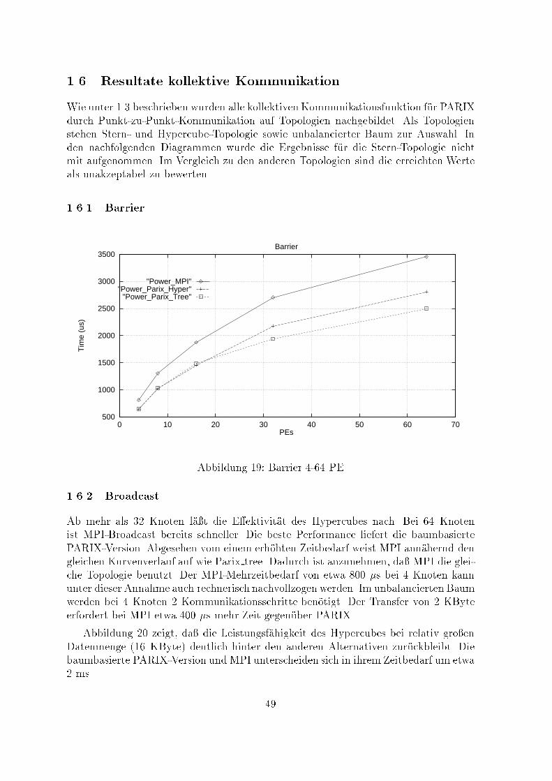
1.6 Resultate kollektive KommunikationWie unter 1.3 beschrieben wurden alle kollektivenKommunikationsfunktion f�ur PARIXdurch Punkt-zu-Punkt-Kommunikation auf Topologien nachgebildet. Als Topologienstehen Stern- und Hypercube-Topologie sowie unbalancierter Baum zur Auswahl. Inden nachfolgenden Diagrammen wurde die Ergebnisse f�ur die Stern-Topologie nichtmit aufgenommen. Im Vergleich zu den anderen Topologien sind die erreichten Werteals unakzeptabel zu bewerten.1.6.1 Barrier500

1000

1500

2000

2500

3000

3500

0 10 20 30 40 50 60 70

Tim

e (u

s)

PEs

Barrier

"Power_MPI""Power_Parix_Hyper"

"Power_Parix_Tree"

Abbildung 19: Barrier 4-64 PE1.6.2 BroadcastAb mehr als 32 Knoten l�a�t die E�ektivit�at des Hypercubes nach. Bei 64 Knotenist MPI-Broadcast bereits schneller. Die beste Performance liefert die baumbasiertePARIX-Version. Abgesehen vom einem erh�ohten Zeitbedarf weist MPI ann�ahernd dengleichen Kurvenverlauf auf wie Parix tree. Dadurch ist anzunehmen, da� MPI die glei-che Topologie benutzt. Der MPI-Mehrzeitbedarf von etwa 800 �s bei 4 Knoten kannunter dieser Annahme auch rechnerisch nachvollzogen werden. Im unbalancierten Baumwerden bei 4 Knoten 2 Kommunikationsschritte ben�otigt. Der Transfer von 2 KByteerfordert bei MPI etwa 400 �s mehr Zeit gegen�uber PARIX.Abbildung 20 zeigt, da� die Leistungsf�ahigkeit des Hypercubes bei relativ gro�enDatenmenge (16 KByte) deutlich hinter den anderen Alternativen zur�uckbleibt. Diebaumbasierte PARIX-Version und MPI unterscheiden sich in ihrem Zeitbedarf um etwa2 ms. 49

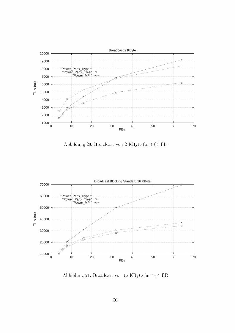
1000

2000

3000

4000

5000

6000

7000

8000

9000

10000

0 10 20 30 40 50 60 70

Tim

e (u

s)

PEs

Broadcast 2 KByte

"Power_Parix_Hyper""Power_Parix_Tree"

"Power_MPI"

Abbildung 20: Broadcast von 2 KByte f�ur 4-64 PE10000

20000

30000

40000

50000

60000

70000

0 10 20 30 40 50 60 70

Tim

e (u

s)

PEs

Broadcast Blocking Standard 16 KByte

"Power_Parix_Hyper""Power_Parix_Tree"

"Power_MPI"

Abbildung 21: Broadcast von 16 KByte f�ur 4-64 PE50

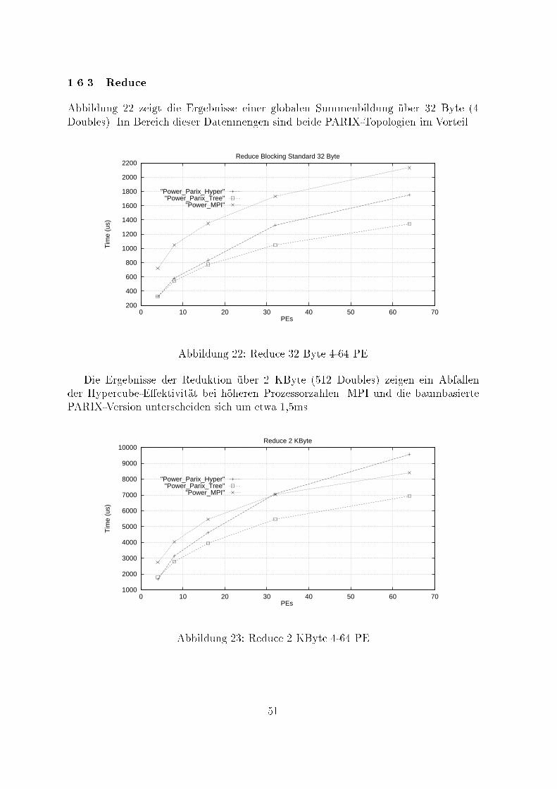
1.6.3 ReduceAbbildung 22 zeigt die Ergebnisse einer globalen Summenbildung �uber 32 Byte (4Doubles). Im Bereich dieser Datenmengen sind beide PARIX-Topologien im Vorteil.200

400

600

800

1000

1200

1400

1600

1800

2000

2200

0 10 20 30 40 50 60 70

Tim

e (u

s)

PEs

Reduce Blocking Standard 32 Byte

"Power_Parix_Hyper""Power_Parix_Tree"

"Power_MPI"

Abbildung 22: Reduce 32 Byte 4-64 PEDie Ergebnisse der Reduktion �uber 2 KByte (512 Doubles) zeigen ein Abfallender Hypercube-E�ektivit�at bei h�oheren Prozessorzahlen. MPI und die baumbasiertePARIX-Version unterscheiden sich um etwa 1,5ms.1000

2000

3000

4000

5000

6000

7000

8000

9000

10000

0 10 20 30 40 50 60 70

Tim

e (u

s)

PEs

Reduce 2 KByte

"Power_Parix_Hyper""Power_Parix_Tree"

"Power_MPI"

Abbildung 23: Reduce 2 KByte 4-64 PE51

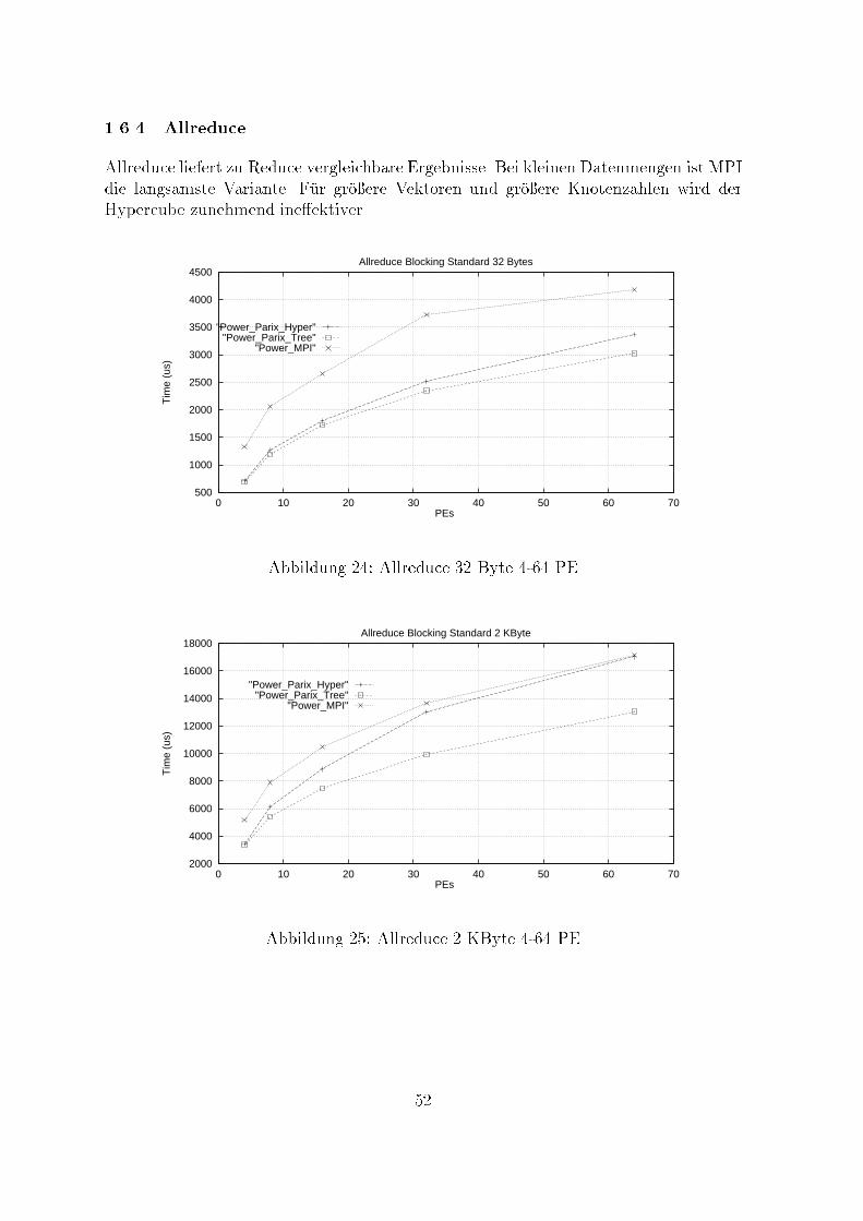
1.6.4 AllreduceAllreduce liefert zu Reduce vergleichbare Ergebnisse. Bei kleinen Datenmengen ist MPIdie langsamste Variante. F�ur gr�o�ere Vektoren und gr�o�ere Knotenzahlen wird derHypercube zunehmend ine�ektiver.500

1000

1500

2000

2500

3000

3500

4000

4500

0 10 20 30 40 50 60 70

Tim

e (u

s)

PEs

Allreduce Blocking Standard 32 Bytes

"Power_Parix_Hyper""Power_Parix_Tree"

"Power_MPI"

Abbildung 24: Allreduce 32 Byte 4-64 PE2000

4000

6000

8000

10000

12000

14000

16000

18000

0 10 20 30 40 50 60 70

Tim

e (u

s)

PEs

Allreduce Blocking Standard 2 KByte

"Power_Parix_Hyper""Power_Parix_Tree"

"Power_MPI"

Abbildung 25: Allreduce 2 KByte 4-64 PE52

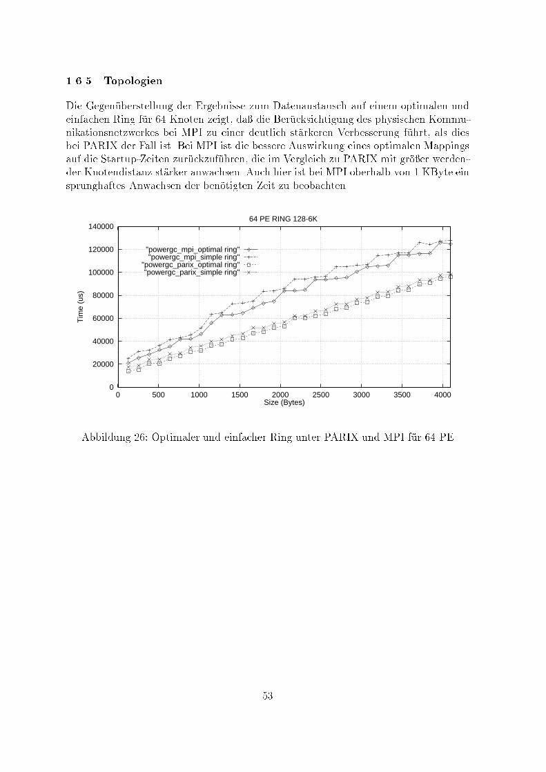
1.6.5 TopologienDie Gegen�uberstellung der Ergebnisse zum Datenaustausch auf einem optimalen undeinfachen Ring f�ur 64 Knoten zeigt, da� die Ber�ucksichtigung des physischen Kommu-nikationsnetzwerkes bei MPI zu einer deutlich st�arkeren Verbesserung f�uhrt, als diesbei PARIX der Fall ist. Bei MPI ist die bessere Auswirkung eines optimalen Mappingsauf die Startup-Zeiten zur�uckzuf�uhren, die im Vergleich zu PARIX mit gr�o�er werden-der Knotendistanz st�arker anwachsen. Auch hier ist bei MPI oberhalb von 1 KByte einsprunghaftes Anwachsen der ben�otigten Zeit zu beobachten.0

20000

40000

60000

80000

100000

120000

140000

0 500 1000 1500 2000 2500 3000 3500 4000

Tim

e (u

s)

Size (Bytes)

64 PE RING 128-6K

"powergc_mpi_optimal ring""powergc_mpi_simple ring"

"powergc_parix_optimal ring""powergc_parix_simple ring"

Abbildung 26: Optimaler und einfacher Ring unter PARIX und MPI f�ur 64 PE53

2 Architekturspezi�scheMPI-Implementierung desEPCC f�ur die CRAY T3DZwischen 1994 und Mai 1995 entwickelten das Edinburgh Parallel Computing Centre(EPCC) und die Firma Cray Research eine eigene Implementierung des MPI-Standardsf�ur die CRAY T3D. Durch die Ber�ucksichtigung spezieller Architektur- und Hardwa-reeigenschaften sollte dem Nutzer unter MPI ein H�ochstma� an Performance gesichertwerden.Auf der Basis der genannten MPI-Implementierung werden Leistungsmessungenf�ur Punkt-zu-Punkt- und kollektive Kommunikation diskutiert und den theoretischverf�ugbaren Leistungsparametern gegen�ubergestellt.2.1 Architektur�ubersicht zur Cray T3DDie Cray T3D ist eine Distributed Memory Multiprozessormaschine, die als nat�urli-ches Speicher- und Programmiermodell jedoch Shared Memory zur Verf�ugung stellt.Die Struktur des Kommunikationsnetzes entspricht einem 3D-Torus. Alle Knoten sind�uber 6 unabh�angige Kan�ale in dieses Netz integriert. Die hardwareseitig verf�ugbareKommunikationsbandbreite wird mit 300 MByte/s angegeben. Jeder Knoten enth�altzwei DEC Alpha 21064 Prozessoren, 64 MB RAM, eine Interconnect-Unit und eineBlock-Transfer-Unit. Die Prozessoren werden mit 150 MHz getaktet, unterst�utzen 64Bit Integer und IEEE Floating Point Operationen und liefern eine Peak-Performancevon je 150 MFlops (64 Bit).Die Logikbausteine au�erhalb der CPU entlasten diese weitgehend von der gesam-ten Kommunikation und erm�oglichen die prinzipielle Sichtweise eines durchg�angigenSpeichers. Praktisch erfolgt der Zugri� auf nichtlokale Speicher �uber vom System be-reitgestellte Kommunikationsprimitive. (shmem get(),shmem put())2.2 Low Level PerformanceF�ur den Zugri� auf den Speicher entfernter Knoten werden die Basisfunktionen shmem put()und shmem get() bereitgestellt. Die Leistungsdaten liegen f�ur shmem get() bei ca 2�sStartup und 60 MByte/s Durchsatz, f�ur shmem put() bei 120 MByte/s Durchsatz beiebenfalls 1-2 �s Startup. Die um den Faktor 2 geringe Bandbreite bei shmem get() istauf den verwendeten �Ubetragungsmechanismus zur�uckzuf�uhren.W�ahrend shmem put()die Daten direkt vom lokalen in den entfernten Speicher �ubertr�agt, bekommt beishmem get() der entfernte Prozessor zun�achst eine Anforderung, durch die er veranla�twird, die gew�unschten Daten zum lokalen Knoten zu �ubertragen.54

2.3 Integration spezieller ArchitektureigenschaftenNutzung atomarer Operationen - Die Behandlung von Anforderungen f�ur Punkt-zu-Punkt-Kommunikation wird in Nachrichten-Queues verwaltet, die dem ge-meinamen Zugri� aller Prozesse unterliegen. Der gegenseitige Ausschlu� der Pro-zesse bei schreibenden Zugri�en auf diese Queue wird mit Hilfe atomarer Ope-rationen realisiert, die durch Prozessor und Speicherverwaltungshardware un-terst�utzt werden (Atomic Swap, Fetch&Increment). Atomic swap tauscht denInhalt eines Registers unmittelbar mit einer Speicheradresse. Fetch&Incrementliest innerhalb einer atomaren Operation den Wert eines speziellen, allgemeinverf�ugbaren Registers, incrementiert diesen und schreibt das Ergebnis zur�uck.Hardwareunterst�utzung f�ur Barrier - Jeder Knoten der T3D besitzt neben denbeiden Prozessoren weitere hochintegrierte Komponenten, die f�ur die Speicher-verwaltung und den gesamten Datentransport verantwortlich sind. Neben die-sen Aufgaben liefern diese Bausteine auch eine e�ziente Hardwareunterst�utzungf�ur Barrier auf der Basis spezieller Register und kaskadierter AND-Gatter. Wer-den alle Knoten einer angeforderten Partition in ein Barrier einbezogen, ist dieAuswertung des Barriers unabh�angig von der Anzahl der teilnehmender Knoteninnerhalb weniger Mikrosekunden (typisch 6 �s) vollzogen. Nehmen nicht alleProzessoren einer Partition an einem Barrier teil, so wird die Barrieroperationsoftwarem�a�ig auf der Basis einer Baumtopologie bearbeitet.Kommunikation auf Basis der Shared Memory Acces Library - Der MPI un-tergeordnete Kommunikationslayer benutzt f�ur den Datenaustausch die Low Le-vel Funktionen shmem put() und shmem get().�Ubertragung kleiner Paketgr�o�en im Nachrichtenheader - Sofern der reine Da-tenbereich einer Nachricht kleiner als 25 Byte ist, wird dieser innerhalb desProtokoll-Headers verschickt. Dadurch er�ubrigt sich die sonst anschlie�ende ei-gentliche Kommunikationssphase.Slotbasierte Verwaltung kollektiver Kommunikation - F�ur die Bearbeitung kol-lektiver Operationen wurde ein Protokollmechanismus implementiert, der auf se-paraten Slots basiert. Als Slot wird ein lokaler Datenbereich bezeichnet, der einemeinzelnen remote Prozessor exklusiv zur Verf�ugung steht, um aktuelle Kommuni-kationsanforderungen zu deponieren. Jeder Prozessor richtet lokal f�ur jeden weite-ren verf�ugbare Prozessor einen solchen Slot ein. Durch die beschriebene Prozessor-Slot-Zuordnung k�onnen zeitaufwendige Lock-Operationen w�ahrend der Behand-lung eines Requestes weitgehend entfallen. Die eigentliche Kommunikation wirdauf Punkt-zu-Punkt-Transfers abgebildet.55

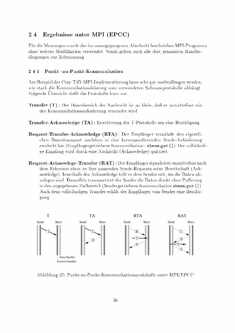
2.4 Ergebnisse unter MPI (EPCC)F�ur die Messungen wurde das im vorangegangenen Abschnitt beschriebenMPI-Programmohne weitere Modi�kation verwendet. Somit gelten auch alle dort genannten Randbe-dingungen zur Zeitmessung.2.4.1 Punkt -zu-Punkt-KommunikationAmBeispiel der Cray T3D-MPI-Implementierung kann sehr gut nochvollzogen werden,wie stark die Kommunikationsleistung vom verwendeten Softwareprotokolle abh�angt.Folgende �Ubersicht stellt die Protokolle kurz vor.Transfer (T) : Der Datenbereich der Nachricht ist so klein, da� er unmittelbar mitder Kommunikationsanforderung versendet wird.Transfer-Acknowledge (TA) : Erweiterung des T-Protokolls um eine Best�atigung.Request-Transfer-Acknowledge (RTA) : Der Empf�anger veranla�t den eigentli-chen Datentransport nachdem er eine korrespondierenden Sende-Anforderungentdeckt hat (Empf�angergetriebeneKommunikation - shmem get()). Der vollst�andi-ge Empfang wird durch eine Nachricht (Acknowledge) quittiert.Request-Acknowlege-Transfer (RAT) : Der Empf�anger signalisiert unmittelbar nachdem Erkennen eines zu ihm passenden Sende-Requests seine Bereitschaft (Ack-nowledge). Innerhalb des Acknowledge teilt er dem Sender mit, wo die Daten ab-zulegen sind. Daraufhin transportiert der Sender die Daten direkt ohne Pu�erungin den angegebenen Zielbereich (Sendergetriebene Kommunikation shmem put()).Nach dem vollst�andigen Transfer erh�alt der Empf�anger vom Sender eine Best�ati-gung.Send Recv

T

Protocol-Handler

Data-Handler

Send Recv

T

A

Send Recv

R

A

Send Recv

T

A

T TA RTA RAT

T

T

AAbbildung 27: Punkt-zu-Punkt-Kommunikationsprotokolle unter MPI/EPCC56

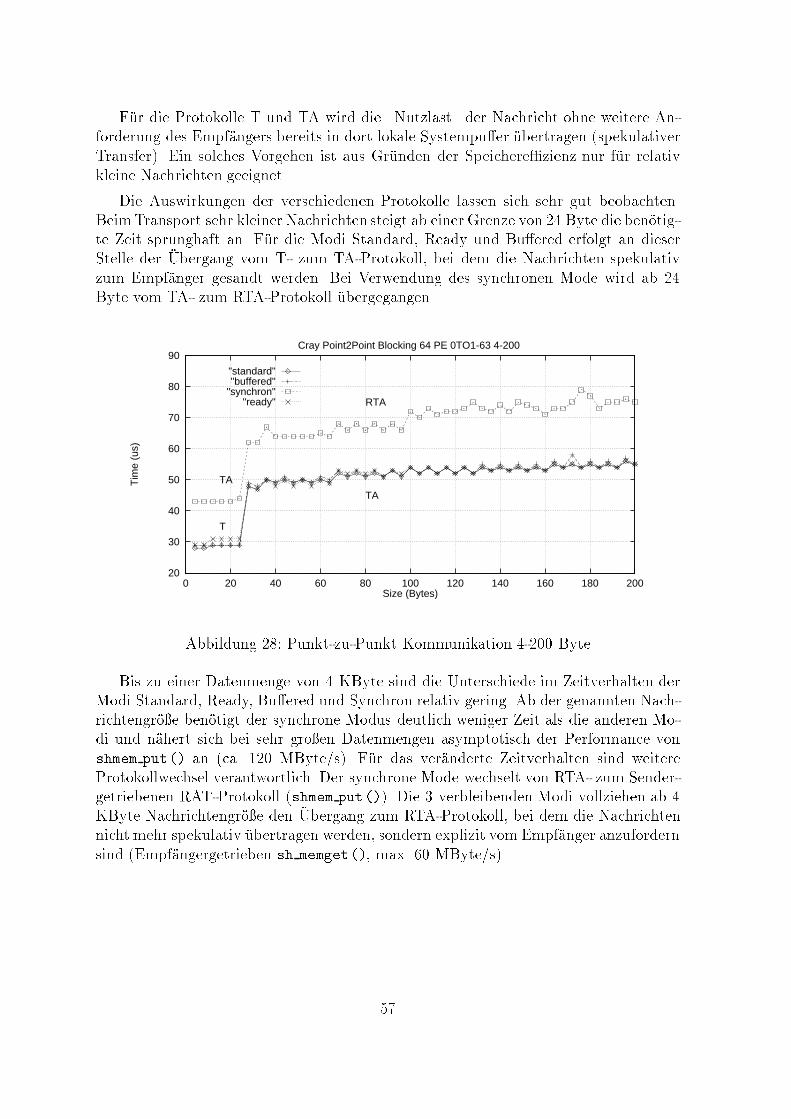
F�ur die Protokolle T und TA wird die \Nutzlast\ der Nachricht ohne weitere An-forderung des Empf�angers bereits in dort lokale Systempu�er �ubertragen (spekulativerTransfer). Ein solches Vorgehen ist aus Gr�unden der Speichere�zienz nur f�ur relativkleine Nachrichten geeignet.Die Auswirkungen der verschiedenen Protokolle lassen sich sehr gut beobachten.BeimTransport sehr kleiner Nachrichten steigt ab einer Grenze von 24 Byte die ben�otig-te Zeit sprunghaft an. F�ur die Modi Standard, Ready und Bu�ered erfolgt an dieserStelle der �Ubergang vom T- zum TA-Protokoll, bei dem die Nachrichten spekulativzum Empf�anger gesandt werden. Bei Verwendung des synchronen Mode wird ab 24Byte vom TA- zum RTA-Protokoll �ubergegangen.20

30

40

50

60

70

80

90

0 20 40 60 80 100 120 140 160 180 200

Tim

e (u

s)

Size (Bytes)

Cray Point2Point Blocking 64 PE 0TO1-63 4-200

T

TA

RTA

TA

"standard""buffered"

"synchron""ready"

Abbildung 28: Punkt-zu-Punkt Kommunikation 4-200 ByteBis zu einer Datenmenge von 4 KByte sind die Unterschiede im Zeitverhalten derModi Standard, Ready, Bu�ered und Synchron relativ gering. Ab der genannten Nach-richtengr�o�e ben�otigt der synchrone Modus deutlich weniger Zeit als die anderen Mo-di und n�ahert sich bei sehr gro�en Datenmengen asymptotisch der Performance vonshmem put() an (ca. 120 MByte/s). F�ur das ver�anderte Zeitverhalten sind weitereProtokollwechsel verantwortlich. Der synchrone Mode wechselt von RTA- zum Sender-getriebenen RAT-Protokoll (shmem put()). Die 3 verbleibenden Modi vollziehen ab 4KByte Nachrichtengr�o�e den �Ubergang zum RTA-Protokoll, bei dem die Nachrichtennicht mehr spekulativ �ubertragen werden, sondern explizit vom Empf�anger anzufordernsind (Empf�angergetrieben sh memget(), max. 60 MByte/s).57

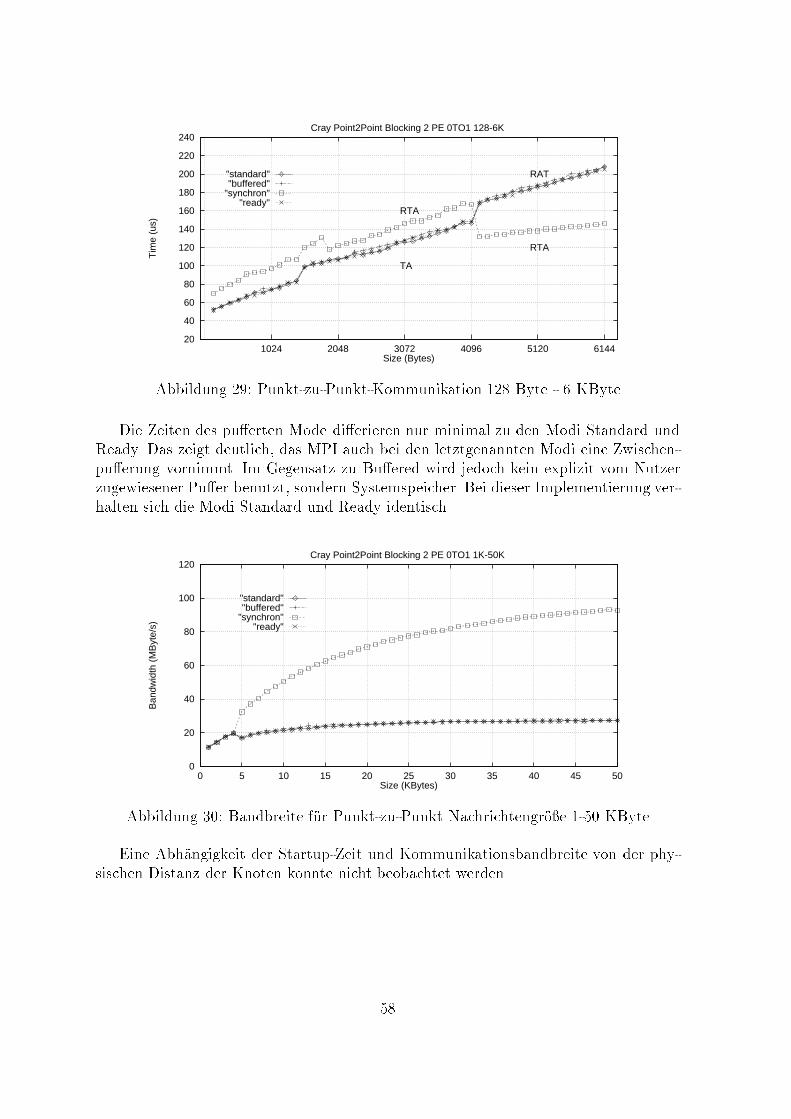
20

40

60

80

100

120

140

160

180

200

220

240

1024 2048 3072 4096 5120 6144

Tim

e (u

s)

Size (Bytes)

Cray Point2Point Blocking 2 PE 0TO1 128-6K

TA

RTA

RTA

RAT"standard""buffered"

"synchron""ready"

Abbildung 29: Punkt-zu-Punkt-Kommunikation 128 Byte - 6 KByteDie Zeiten des pu�erten Mode di�erieren nur minimal zu den Modi Standard undReady. Das zeigt deutlich, das MPI auch bei den letztgenannten Modi eine Zwischen-pu�erung vornimmt. Im Gegensatz zu Bu�ered wird jedoch kein explizit vom Nutzerzugewiesener Pu�er benutzt, sondern Systemspeicher. Bei dieser Implementierung ver-halten sich die Modi Standard und Ready identisch.0

20

40

60

80

100

120

0 5 10 15 20 25 30 35 40 45 50

Ban

dwid

th (

MB

yte/

s)

Size (KBytes)

Cray Point2Point Blocking 2 PE 0TO1 1K-50K

"standard""buffered"

"synchron""ready"

Abbildung 30: Bandbreite f�ur Punkt-zu-Punkt Nachrichtengr�o�e 1-50 KByteEine Abh�angigkeit der Startup-Zeit und Kommunikationsbandbreite von der phy-sischen Distanz der Knoten konnte nicht beobachtet werden.58

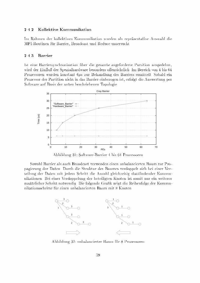
2.4.2 Kollektive KommunikationIm Rahmen der kollektiven Kommunikation wurden als repr�asentative Auswahl dieMPI-Routinen f�ur Barrier, Broadcast und Reduce untersucht.2.4.3 BarrierIst eine Barriersynchronisation �uber die gesamte angeforderte Partition ausgedehnt,wird der Ein u� der Spezialhardware besonders o�ensichtlich. Im Bereich von 4 bis 64Prozessoren wurden konstant 6�s zur Behandlung des Barriers ermittelt. Sobald einProzessor der Partition nicht in das Barrier einbezogen ist, erfolgt die Auswertung perSoftware auf Basis der unten beschriebenen Topologie.0

5

10

15

20

25

30

35

0 10 20 30 40 50 60 70

Tim

e (u

s)

PEs

Cray Barrier

"Software_Barrier""Hardware_Barrier"

Abbildung 31: Software-Barrier 4 bis 64 ProzessorenSowohl Barrier als auch Broadcast verwenden einen unbalancierten Baum zur Pro-pagierung der Daten. Durch die Struktur des Baumes verdoppelt sich bei einer Ver-teilung der Daten mit jedem Schritt die Anzahl gleichzeitig statt�ndender Kommu-nikationen. Bei einer Verdoppelung der beteiligten Knoten ist somit nur ein weitererzus�atzlicher Schritt notwendig. Die folgende Gra�k zeigt die Reihenfolge der Kommu-nikationsschritte f�ur einen unbalancierten Baum mit 8 Knoten.1

2

3

2

3

3

3

1

2

2

3 1

1

1Abbildung 32: unbalancierter Baum f�ur 8 Prozessoren59

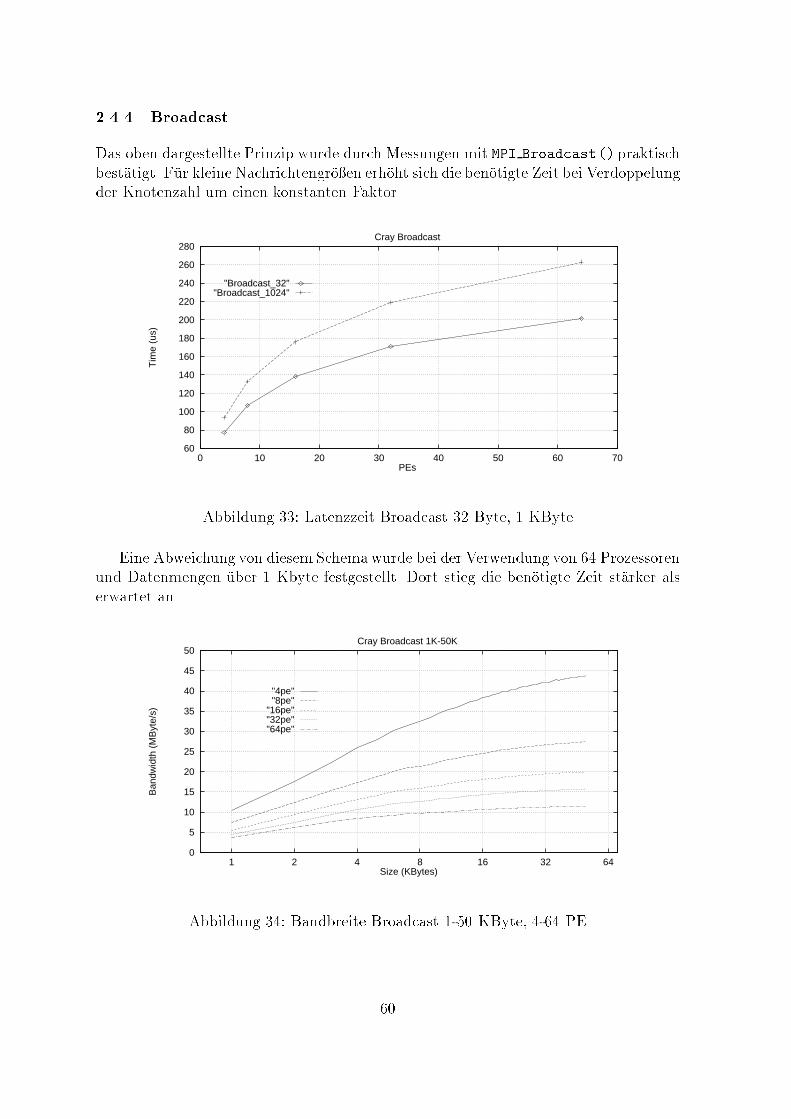
2.4.4 BroadcastDas oben dargestellte Prinzip wurde durch Messungen mit MPI Broadcast() praktischbest�atigt. F�ur kleine Nachrichtengr�o�en erh�oht sich die ben�otigte Zeit bei Verdoppelungder Knotenzahl um einen konstanten Faktor.60

80

100

120

140

160

180

200

220

240

260

280

0 10 20 30 40 50 60 70

Tim

e (u

s)

PEs

Cray Broadcast

"Broadcast_32""Broadcast_1024"

Abbildung 33: Latenzzeit Broadcast 32 Byte, 1 KByteEine Abweichung von diesem Schemawurde bei der Verwendung von 64 Prozessorenund Datenmengen �uber 1 Kbyte festgestellt. Dort stieg die ben�otigte Zeit st�arker alserwartet an.0

5

10

15

20

25

30

35

40

45

50

1 2 4 8 16 32 64

Ban

dwid

th (

MB

yte/

s)

Size (KBytes)

Cray Broadcast 1K-50K

"4pe""8pe"

"16pe""32pe""64pe"

Abbildung 34: Bandbreite Broadcast 1-50 KByte, 4-64 PE60

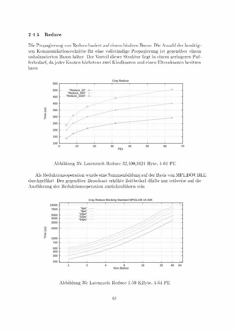
2.4.5 ReduceDie Propagierung von Reduce basiert auf einem bin�aren Baum. Die Anzahl der ben�otig-ten Kommunikationsschritte f�ur eine vollst�andige Propagierung ist gegen�uber einemunbalancierten Baum h�oher. Der Vorteil dieser Struktur liegt in einem geringeren Puf-ferbedarf, da jeder Knoten h�ochstens zwei Kindknoten und einen Elternknoten besitzenkann.100

150

200

250

300

350

400

450

500

550

0 10 20 30 40 50 60 70

Tim

e (u

s)

PEs

Cray Reduce

"Reduce_32""Reduce_400"

"Reduce_1024"

Abbildung 35: Latenzzeit Reduce 32,400,1024 Byte, 4-64 PEAls Reduktionsoperation wurde eine Summenbildung auf der Basis vonMPI DOUBLEdurchgef�uhrt. Der gegen�uber Broadcast erh�ohte Zeitbedarf d�urfte nur teilweise auf dieAusf�uhrung der Reduktionsoperation zur�uckzuf�uhren sein.200

300

400500

750

1000

2000

3000

40005000

7500

10000

1 2 4 8 16 32 48 64

Tim

e (u

s)

Size (Bytes)

Cray Reduce Blocking Standard MPIGLOB 1K-50K

"4pe""8pe"

"16pe""32pe""64pe"

Abbildung 36: Latenzzeit Reduce 1-50 KByte, 4-64 PE61

2.4.6 Schlu�bemerkungAn dieser Stelle sei den Kollegen des Conrad-Zuse-Instituts Berlin gedankt, die inner-halb kurzer Zeit und erfreulich unb�urokratisch den Zugang zur dort installierten CrayT3D-256 erm�oglichten und halfen, erste Anfangsh�urden zu �uberwinden.Literatur[1] S. Burkhardt u.a., Parallele Rechnersysteme - Programmierung und Anwendung,Verlag Technik GmbH, Berlin M�unchen, 1993[2] Message Passing Interface Forum, DRAFT Document for a Standard Message Pas-sing Interface, Stand 30.6.93, 1993[3] A. Geist u.a., PVM 3.0 user's guide and reference manual, Oak Ridge NationalLaboratory, Feb. 93[4] V.Karamcheti u.a. , FM: Fast Messaging on the Cray T3D, University of Illinois atUrbana-Champaign, Department of Computer Science, 1995[5] J.J. Dongarra, T. Dunigan, Message-Passing Performance of various Computers,Oak Ridge National Laboratory, Computer Science and Mathematics Division, 1996[6] K. Cameron, L. C. Clarke, A.G. Smith, Using MPI on the Cray T3D, EdinburghParallel Computing Centre, 1995[7] K. Cameron, L. C. Clarke, A.G. Smith, CRI/EPCC MPI for Cray T3D, EdinburghParallel Computing Centre, Edinburgh EH9 3JZ, 1995[8] Cray Research, Inc. , Cray T3D System Architecture Overview, March 199362

Message Passing E�ciency on Shared MemoryArchitecturesThomas Radketomsoft@informatik.tu-chemnitz.dehttp://noah.informatik.tu-chemnitz.de/members/radke/radke.html1 IntroductionEspecially in the framework of the newly founded "Sonderforschungsbereich SFB 393 :Numerische Simulation auf massiv parallelen Rechnern", other parallel architectures {namely shared memory systems { are to be investigated for their ability to e�cientlysolve the addressed problems. Two principle ways are possible to implement parallelprograms on shared memory architectures. First, one can use multithreading as thebasic programming model for his/her implementation[1]. This guarantees the best useof the facilities of the underlying hardware. The other way is to use a message passinginterface, that resides on top of multithreading, and write a CSP program.The �rst way was evaluated at our department by porting a module of an exist-ing message passing program (FEM solver) onto a shared memory system[2]. Testsshowed that good e�ciency results can be obtained for small problem sizes mappedonto few processors. But the port took a considerable amount of time, and writing amultithreaded program appeared to be even harder than de�ning the same problemwith the message passing paradigm.As there are comprehensive experiences at the University of Technology Chemnitzwith message passing programming on the Parsytec massively parallel computer series,we concluded that the second approach should be favourized in the SFB 393.This paper describes the potential facilities for message passing on 2 shared mem-ory systems available at the Department of Computer Science: the KSR1 from KendallSqare Research, and Compaq's ProLiant 4000. The theoretical e�ciencies of a mes-sage passing interface are given as communication bandwidth, communication latency,parallelity of communication and computation, and the implementation of global op-erations. E�cieny losses due to the implementation of the underlying multithreadingfunctionality are not studied here in detail, the main intention was to evaluate theshared memory hardware architecture.63

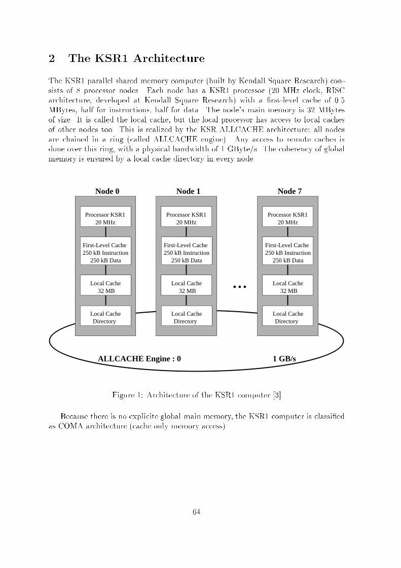
2 The KSR1 ArchitectureThe KSR1 parallel shared memory computer (built by Kendall Square Research) con-sists of 8 processor nodes. Each node has a KSR1 processor (20 MHz clock, RISCarchitecture, developed at Kendall Square Research) with a �rst-level cache of 0.5MBytes, half for instructions, half for data. The node's main memory is 32 MBytesof size. It is called the local cache, but the local processor has access to local cachesof other nodes too. This is realized by the KSR ALLCACHE architecture: all nodesare chained in a ring (called ALLCACHE engine). Any access to remote caches isdone over this ring, with a physical bandwidth of 1 GByte/s. The coherency of globalmemory is ensured by a local cache directory in every node....

ALLCACHE Engine : 0 1 GB/s

Node 0 Node 1 Node 7

Processor KSR1

First-Level Cache250 kB Instruction

20 MHz

32 MBLocal Cache

Processor KSR1

First-Level Cache250 kB Instruction

20 MHz

32 MBLocal Cache

Local Cache Local Cache

Processor KSR1

First-Level Cache250 kB Instruction

20 MHz

32 MBLocal Cache

Local CacheDirectory Directory Directory

250 kB Data250 kB Data 250 kB Data

Figure 1: Architecture of the KSR1 computer [3]Because there is no explicite global main memory, the KSR1 computer is classi�edas COMA architecture (cache only memory access).64

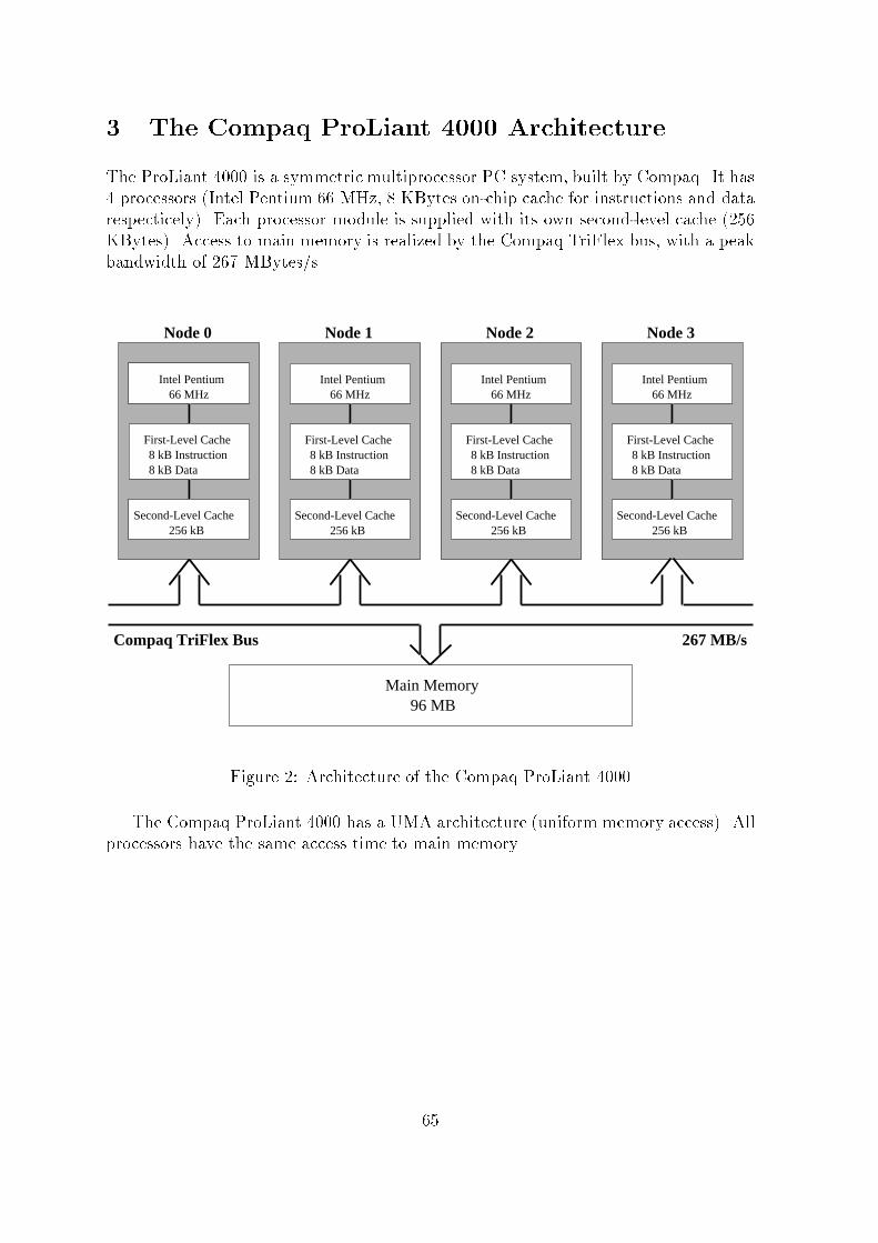
3 The Compaq ProLiant 4000 ArchitectureThe ProLiant 4000 is a symmetric multiprocessor PC system, built by Compaq. It has4 processors (Intel Pentium 66 MHz, 8 KBytes on-chip cache for instructions and datarespecticely). Each processor module is supplied with its own second-level cache (256KBytes). Access to main memory is realized by the Compaq TriFlex bus, with a peakbandwidth of 267 MBytes/s.Compaq TriFlex Bus 267 MB/s

Node 0 Node 1 Node 2 Node 3

Main Memory96 MB

Intel Pentium66 MHz

First-Level Cache8 kB Instruction8 kB Data

256 kBSecond-Level Cache

Intel Pentium66 MHz

First-Level Cache8 kB Instruction8 kB Data

256 kBSecond-Level Cache Second-Level Cache

Intel Pentium66 MHz

First-Level Cache8 kB Instruction8 kB Data

256 kBSecond-Level Cache

Intel Pentium66 MHz

First-Level Cache8 kB Instruction8 kB Data

256 kB

Figure 2: Architecture of the Compaq ProLiant 4000The Compaq ProLiant 4000 has a UMA architecture (uniform memory access). Allprocessors have the same access time to main memory.65

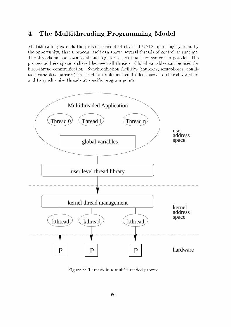
4 The Multithreading Programming ModelMultithreading extends the process concept of classical UNIX operating systems bythe opportunity, that a process itself can spawn several threads of control at runtime.The threads have an own stack and register set, so that they can run in parallel. Theprocess address space is shared between all threads. Global variables can be used forinter-thread-communication. Synchronization facilities (mutexes, semaphores, condi-tion variables, barriers) are used to implement controlled access to shared variablesand to synchronize threads at speci�c program points.

P P P

user level thread library

useraddressspace

kernel thread management

Thread 0 Thread 1 Thread n

global variables

addresskernel

spacekthread kthread kthread

hardware

Multithreaded Application

Figure 3: Threads in a multithreaded process66

5 Message Passing on Top of MultithreadingThe emulation of message passing in a multithreaded environment can be expressed asfollowing:� Threads become the nodes of the message passing program.� Communication is done via synchronization of threads and simply copying of thedata from the sending node to the receiver.5.1 Threads as NodesIn distinction to message passing programming under PARIX, where the whole mainprogram is duplicated onto all processor nodes at load time, threads begin their execu-tion in a start function from within the same process. This could be done implicitelyby calling a functionint MP_Init (unsigned int num_nodes, void (*start_fn) (void *arg));with start fn specifying the function to start execution of the thread with the singleargument arg, and num nodes determining the number of nodes to create.Another distinction is the declaration of global variables. In a PARIX program, allglobal variables are visible to the local node only. In multithreaded programs thesevariables are shared between all nodes. A possible way to solve this problem is theintroduction of private data. Each variable with an attribute private becomes thread-speci�c, i.e., every thread gets a local copy of the variable. This solution requiresthe explicite declaration of those variables by the application programmer and somechanges in the compiler to support the handling with thread-speci�c data.5.2 Node-to-Node CommunicationCommunication between nodes is very easy to implement because of the common ad-dress space of all threads. A (synchronous) communication operation requires thesynchronization of the participating nodes and a data transfer operation (a simplememcpy) from the sender to the receiver(s).Prototypes for a basic SendMessage() / RecvMessage() function are introducedin the following:typedef struct {sem_t sendReady, recvReady;void *message;unsigned int bytes;unsigned int *transfered; 67

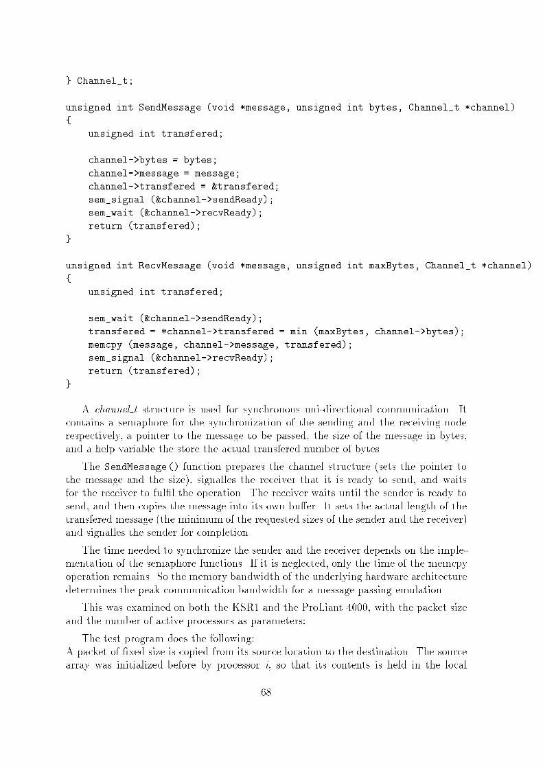
} Channel_t;unsigned int SendMessage (void *message, unsigned int bytes, Channel_t *channel){ unsigned int transfered;channel->bytes = bytes;channel->message = message;channel->transfered = &transfered;sem_signal (&channel->sendReady);sem_wait (&channel->recvReady);return (transfered);}unsigned int RecvMessage (void *message, unsigned int maxBytes, Channel_t *channel){ unsigned int transfered;sem_wait (&channel->sendReady);transfered = *channel->transfered = min (maxBytes, channel->bytes);memcpy (message, channel->message, transfered);sem_signal (&channel->recvReady);return (transfered);} A channel t structure is used for synchronous uni-directional communication. Itcontains a semaphore for the synchronization of the sending and the receiving noderespectively, a pointer to the message to be passed, the size of the message in bytes,and a help variable the store the actual transfered number of bytes.The SendMessage() function prepares the channel structure (sets the pointer tothe message and the size), signalles the receiver that it is ready to send, and waitsfor the receiver to ful�l the operation. The receiver waits until the sender is ready tosend, and then copies the message into its own bu�er. It sets the actual length of thetransfered message (the minimum of the requested sizes of the sender and the receiver)and signalles the sender for completion.The time needed to synchronize the sender and the receiver depends on the imple-mentation of the semaphore functions. If it is neglected, only the time of the memcpyoperation remains. So the memory bandwidth of the underlying hardware architecturedetermines the peak communication bandwidth for a message passing emulation.This was examined on both the KSR1 and the ProLiant 4000, with the packet sizeand the number of active processors as parameters:The test program does the following:A packet of �xed size is copied from its source location to the destination. The sourcearray was initialized before by processor i, so that its contents is held in the local68

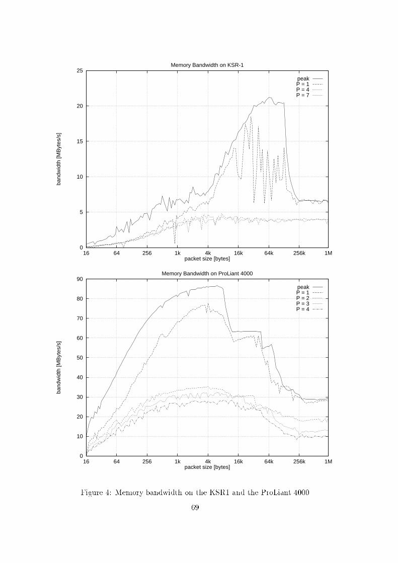
0

5

10

15

20

25

16 64 256 1k 4k 16k 64k 256k 1M

band

wid

th [M

Byt

es/s

]

packet size [bytes]

Memory Bandwidth on KSR-1

peakP = 1P = 4P = 7

0

10

20

30

40

50

60

70

80

90

16 64 256 1k 4k 16k 64k 256k 1M

band

wid

th [M

Byt

es/s

]

packet size [bytes]

Memory Bandwidth on ProLiant 4000

peakP = 1P = 2P = 3P = 4

Figure 4: Memory bandwidth on the KSR1 and the ProLiant 400069

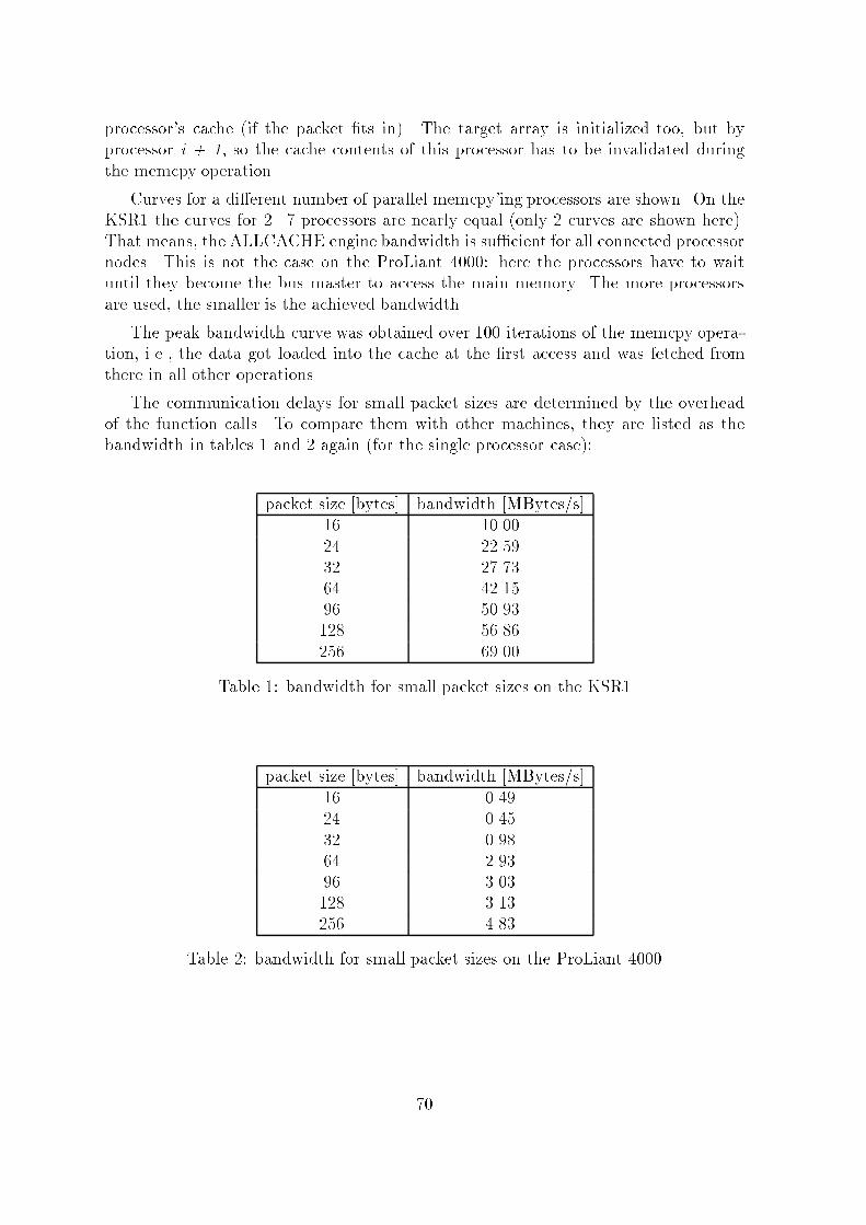
processor's cache (if the packet �ts in). The target array is initialized too, but byprocessor i + 1, so the cache contents of this processor has to be invalidated duringthe memcpy operation.Curves for a di�erent number of parallel memcpy'ing processors are shown. On theKSR1 the curves for 2...7 processors are nearly equal (only 2 curves are shown here).That means, the ALLCACHE engine bandwidth is su�cient for all connected processornodes. This is not the case on the ProLiant 4000: here the processors have to waituntil they become the bus master to access the main memory. The more processorsare used, the smaller is the achieved bandwidth.The peak bandwidth curve was obtained over 100 iterations of the memcpy opera-tion, i.e., the data got loaded into the cache at the �rst access and was fetched fromthere in all other operations.The communication delays for small packet sizes are determined by the overheadof the function calls. To compare them with other machines, they are listed as thebandwidth in tables 1 and 2 again (for the single processor case):packet size [bytes] bandwidth [MBytes/s]16 10.0024 22.5932 27.7364 42.1596 50.93128 56.86256 69.00Table 1: bandwidth for small packet sizes on the KSR1packet size [bytes] bandwidth [MBytes/s]16 0.4924 0.4532 0.9864 2.9396 3.03128 3.13256 4.83Table 2: bandwidth for small packet sizes on the ProLiant 400070

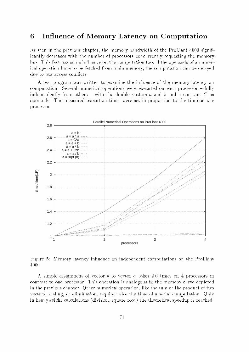
6 In uence of Memory Latency on ComputationAs seen in the previous chapter, the memory bandwidth of the ProLiant 4000 signif-icantly decreases with the number of processors concurrently requesting the memorybus. This fact has some in uence on the computation too: if the operands of a numer-ical operation have to be fetched from main memory, the computation can be delayeddue to bus access con icts.A test program was written to examine the in uence of the memory latency oncomputation. Several numerical operations were executed on each processor { fullyindependently from others { with the double vectors a and b and a constant C asoperands. The measured execution times were set in proportion to the time on oneprocessor.

1

1.2

1.4

1.6

1.8

2

2.2

2.4

2.6

2.8

1 2 3 4

time

/ tim

e(1P

)

processors

Parallel Numerical Operations on ProLiant 4000

a = ba = a * aa = C*a

a = a + ba = a * b

a = a + C*ba = a / b

a = sqrt (b)

Figure 5: Memory latency in uence on independent computations on the ProLiant4000A simple assignment of vector b to vector a takes 2.6 times on 4 processors incontrast to one processor. This operation is analogous to the memcpy curve depictedin the previous chapter. Other numerical operation, like the sum or the product of twovectors, scaling, or elimination, require twice the time of a serial computation. Onlyin heavyweight calculations (division, square root) the theoretical speedup is reached.71

7 Global OperationsTo examine the e�ciency of global operations, two algorithms for the computation ofa global sum of double vectors were implemented:� a serial version with barrier synchronizationThe �rst thread that enters the barrier initializes a global operation structureby setting the pointer to its local vector to an intermediate result pointer, andsuspends its execution to wait for the other threads. These add their own vectorto the intermediate sum vector (the vector of the �rst thread is used for this) asthey reach the barrier, and suspend themselfes too. The last thread computesthe �nal sum vector and then awakenes all suspended threads by a broadcast onthe barrier. Now all threads copy the result into its own local result vector.� a parallel version via hypercube communicationA hypercube topology is used to exchange the vectors between adjacent nodes.Both the local and the remote vector are added and sent to the next neighbour.This version has a parallelity degree of D (the dimension of the hypercube).

72

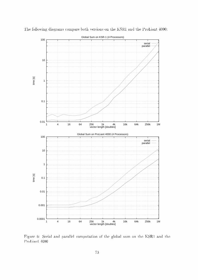
The following diagrams compare both versions on the KSR1 and the ProLiant 4000:0.01

0.1

1

10

100

1 4 16 64 256 1k 4k 16k 64k 256k 1M

time

[s]

vector length [doubles]

Global Sum on KSR-1 (4 Processors)

serialparallel

0.0001

0.001

0.01

0.1

1

10

100

1 4 16 64 256 1k 4k 16k 64k 256k 1M

time

[s]

vector length [doubles]

Global Sum on ProLiant 4000 (4 Processors)

serialparallel

Figure 6: Serial and parallel computation of the global sum on the KSR1 and theProLiant 4000 73

As can be seen, the serial algorithm works faster than the parallel one on bothmachines. There might be two reasons for that: at �rst, the global sum is a verycheap numerical operation (see �gure 6). More complex operation should bring bothcurves nearer to each other. And secondly, only 4 processors were used (there werenot more processors available on the KSR1 to build a hypercube of dimension 3). Themore processors calculate in parallel the higher should be the speedup of the parallelalgorithm.8 ConclusionsThe communication bandwidth achieved in a message passing emulation on sharedmemory architectures is mainly determined by their memory bandwidth and thereforeis often much higher compared with distributed memory architectures. An importantdemand to the memory system is scalability: a processor's access to global memoryshould not be delayed by concurrent independent accesses of other processors. Theuse of local processor caches signi�cantly increases the speedup, so caches should be aslarge as possible.Computations should contain complex operations rather than simple, if the mem-ory bandwidth of the underlying architecture is not su�cient for parallel work of allprocessors. Otherwise a decrease of speedup is the consequence, even if the operationsare fully independently of each other.For global operations there exists a break-even point, where a serial implementationis still faster than a parallel one (based on the model of true message passing imple-mentations, e.g. hypercube communication). There are very e�cient global synchro-nization methods for threads (e.g. barriers) which can overweigh the parallel versionswith their several local synchronizations.References[1] T. Radke. Parallel Programming with User-level Threads, Technical Report TUCZ/ RA-TR-96-3, Computer Science Department, University of Technology Chem-nitz, 1996.[2] L. Grabowsky. Parallel FEM implementations on shared memory systems, Tech-nical Report TUCZ / RA-TR-96-4, Computer Science Department, University ofTechnology Chemnitz, 1996.[3] KSR1 Principles of Operations, Kendall Square Research Corporation, Mas-sachusetts, 1993.[4] PentiumTM Processor User's Manual, Intel Corporation, 1994.74

MPI-Portierung eines FEM-ProgrammesUwe Beyer Andreas Munkeube@informatik.tu-chemnitz.de ambu@informatik.tu-chemnitz.dehttp://noah.informatik.tu-chemnitz.de/members/beyer/beyer.html http://noah.informatik.tu-chemnitz.de/members/munke/munke.htmlZusammenfassungIm Rahmen der Leistungsanalyse des Message Passing Interface (MPI) wurdeein Programm zur L�osung von 2-dimensionalen Potentialproblemen, welches aufder Finiten-Elemente-Methode (FEM) basiert, auf PowerMPI portiert. Ausge-hend von dieser praktischen Erfahrung werden Erkenntnisse �uber die Handhab-barkeit von MPI, den entstandenen Programmieraufwand und das Laufzeitver-halten der MPI-Version des Programmes abgeleitet.1 ZielstellungBei den Untersuchungen eines neuen Programmierwerkzeuges, einer verbesserten Rech-nerarchitektur oder eines innovativen Standards hinsichtlich der Leistungsmerkmale,Funktionalit�at und Verwendbarkeit werden sehr oft spezielle und zugeschnittene Testsdurchgef�uhrt. Die Resultate einer solchen Analyse sind daher meist aussagekr�aftigeund konkrete Werte, anhand derer es m�oglich ist, das untersuchte Objekt zu bewertenund eventuell mit vergleichbaren Objekten in Relation setzen zu k�onnen. Bei diesenUntersuchungen kommt es darauf an, de�nierte Bedingungen zu scha�en, um einzel-ne Parameter oder das Zusammenspiel mehrerer Parameter gezielt zu steuern und dieReaktionen des Systems zu ermitteln. Neben der direkt me�baren Performance des zuuntersuchenden Objektes stehen aber auch dessen Eigenschaften bei der Ausf�uhrungeiner realen und komplexen Aufgabe im Vordergrund der Betrachtungen. Interessantund wichtig ist dies, da bei einem sp�ateren praktischen Einsatz nicht mehr das Ob-jekt selbst, sondern nur noch die L�osung eines Problems im Mittelpunkt steht. Dasuntersuchte System hat dann ausschlie�lich seine Funktion zu erf�ullen und sich in dasGesamtprojekt zu integrieren. Eine Leistungsanalyse sollte daher auch den n�otigenAufwand bei einem Einsatz, die auftretenden Probleme und das Laufzeitverhalten inkomplexen Applikationen ermitteln, um praktische Erfahrungen im Umgang mit demObjekt zu gewinnen.Vor diesem Hintergrund entstand im Rahmen der Leistungsanalyse des MessagePassing Interface-Standards (MPI) die Aufgabe, die existierende PARIX-Version desProgrammes SPC-PMPo2 auf MPI zu portieren. Diese Applikation ist ein Programmzur parallelen L�osung von 2-dimensionalen Potentialproblemen auf der algorithmischenBasis der Finiten-Elemente-Methode (FEM). Sowohl das Programm selbst als auch dieunterst�utzenden Bibliotheken wurden an der Fakult�at f�ur Mathematik der TechnischenUniversit�at Chemnitz-Zwickau von der Arbeitsgruppe \Scienti�c Parallel Computing"entwickelt. 75

Von dem Erstellen der MPI-Version dieses Programmes wurden nun exemplarischeAussagen �uber die Handhabbarkeit von MPI und den n�otigen Aufwand zur L�osungdieser Aufgabe erwartet. Desweiteren sollten Laufzeitvergleiche zwischen den beidenVarianten Auskunft �uber den Geschwindigkeitsnachteil der MPI-Realisierung geben.Zu beachten ist hierbei nat�urlich, da� die ermittelten Resultate nicht den Vorteil derAllgemeing�ultigkeit besitzen. Daf�ur stellen sie aber die Erfahrungen �uber den Umgangmit MPI bei der L�osung einer konkreten Aufgabe dar und k�onnen somit als Richtwertf�ur vergleichbare Projekte dienen.2 Portabilit�at paralleler ApplikationenEin bedeutendes Problem bei der Entwicklung von parallelen Applikationen sind dieSchwierigkeiten beim Scha�en von portablen Projekten. Das hei�t von Programmenoder Bibliotheken, die ohne gro�en Aufwand auf mehreren unterschiedlichen, paralle-len Rechnersystemen abgearbeitet werden k�onnen. Komplikationen bereiten hierbei dieverschiedenen Konzepte f�ur den Zugang der Applikation zum Kommunikationssystemdes Rechners. Dieser Zugang ist insbesondere bei Systemen die auf dem Nachrichten-austausch (Message-Passing) zwischen Prozessorknoten beruhen, von grundlegenderBedeutung. Aber gerade die Kommunikationrufe an die jeweilige Hardware unterschei-den sich durch das Fehlen von hersteller�ubergreifenden Standards. Damit mu� eine por-table Applikation oder ein Bibliothekspaket immer eine Schicht f�ur die Anpassung andie Gegebenheiten der entsprechenden Parallelrechnersysteme enthalten. Diese Anpas-sungsschicht mu� im Normalfall bei jeder Portierung auf einen anderen Parallelrechnerneu implementiert werden. Um den daf�ur notwendigen Aufwand gering zu halten, wirdoft die Funktionalit�at des architekturspezi�schen \Bindegliedes" sehr klein gehaltenund auf grundlegende Funktionen beschr�ankt. Alle ben�otigten komplexeren Routinen,wie zum Beispiel globale Kommunikationsrufe, m�ussen nun innerhalb der Applika-tion oder Bibliothek auf dieses kleine Interface abgebildet werden, welches mit denKommunikationsprimiven des Parallelrechners arbeitet. Sollten vergleichbare komple-xere Funktionen auch von dem Rechnersystem angeboten werden, so ist es dann nichtm�oglich diese zu verwenden. Dies verursacht einerseits einen deutlich erh�ohten Pro-grammieraufwand und andererseits bei den mei�ten Systemen einen Laufzeitverlu�t,da die komplexen, systeminternen Funktionen e�zienter auf die Hardware abgebildetwerden k�onnen, als es bei den selbstgeschriebenen m�oglich ist.Mit dem Formulieren und Implementieren des Message Passing Interface-Standardswurde ein system�ubergreifendes Werkzeug gescha�en, mit dem es in Zukunft m�oglichsein wird, parallele Programme zu erstellen, die auf eine Anpassung an die spezielleArchitektur verzichten k�onnen. Der Programmierer arbeitet hierbei mit architekturu-nabh�angigen, von der MPI-Bibliothek zu Verf�ugung gestellten Kommunikationsfunk-tionen. Die Anpassung an die Spezi�ka der aktuellen Umgebung wird nun von MPI�ubernommen. Der Anwendungsprogrammierer mu� lediglich die MPI-Bibliothek f�urdie zu bearbeitende Architektur zur Verf�ugung stellen und kann die Applikation ohne�Anderung des Quelltextes auf verschiedenen Parallelrechnerarchitekturen abarbeiten.76

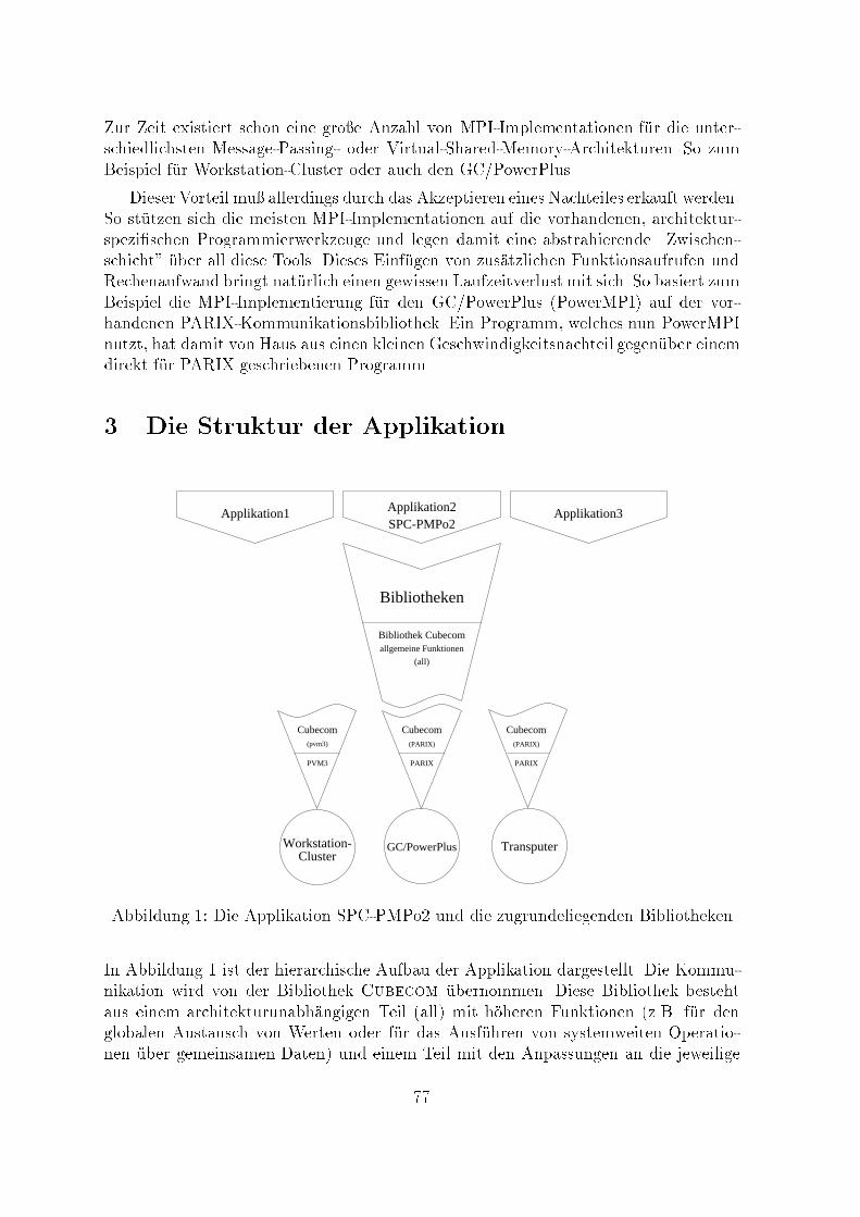
Zur Zeit existiert schon eine gro�e Anzahl von MPI-Implementationen f�ur die unter-schiedlichsten Message-Passing- oder Virtual-Shared-Memory-Architekturen. So zumBeispiel f�ur Workstation-Cluster oder auch den GC/PowerPlus.Dieser Vorteil mu� allerdings durch das Akzeptieren eines Nachteiles erkauft werden.So st�utzen sich die meisten MPI-Implementationen auf die vorhandenen, architektur-spezi�schen Programmierwerkzeuge und legen damit eine abstrahierende \Zwischen-schicht" �uber all diese Tools. Dieses Einf�ugen von zus�atzlichen Funktionsaufrufen undRechenaufwand bringt nat�urlich einen gewissen Laufzeitverlust mit sich. So basiert zumBeispiel die MPI-Implementierung f�ur den GC/PowerPlus (PowerMPI) auf der vor-handenen PARIX-Kommunikationsbibliothek. Ein Programm, welches nun PowerMPInutzt, hat damit von Haus aus einen kleinen Geschwindigkeitsnachteil gegen�uber einemdirekt f�ur PARIX geschriebenen Programm.3 Die Struktur der ApplikationApplikation1 Applikation2

SPC-PMPo2Applikation3

PVM3 PARIX

Bibliotheken

Bibliothek Cubecomallgemeine Funktionen

(all)

Cubecom Cubecom Cubecom(pvm3) (PARIX)

PARIX

Workstation- Transputer

(PARIX)

ClusterGC/PowerPlusAbbildung 1: Die Applikation SPC-PMPo2 und die zugrundeliegenden BibliothekenIn Abbildung 1 ist der hierarchische Aufbau der Applikation dargestellt. Die Kommu-nikation wird von der Bibliothek Cubecom �ubernommen. Diese Bibliothek bestehtaus einem architekturunabh�angigen Teil (all) mit h�oheren Funktionen (z.B. f�ur denglobalen Austausch von Werten oder f�ur das Ausf�uhren von systemweiten Operatio-nen �uber gemeinsamen Daten) und einem Teil mit den Anpassungen an die jeweilige77

Plattform. Der architekturspezi�sche Teil wird durch wenige, primitive Kommunikati-onsfunktionen �ubernommen, f�ur die eine einheitliche Schnittstelle de�niert wurde. DieFunktionalit�at dieses Teiles besteht haupts�achlich aus Funktionen f�ur die Initialisierungund den Abbau der Kommunikation sowie aus Routinen f�ur das Senden einer Anzahlvon Worten an einen bestimmten, direktadressierten Knoten, oder �uber einen Link derzugrundeliegenden HyperCube-Topologie. F�ur die Portierung des FEM-Programmes,oder allgemeiner: der Bibliotheken, war es dadurch ausreichend, die Funktionen desspezi�schen Teils zu modi�zieren oder neu zu implementieren. Durch diese Herange-hensweise wird die MPI-Version des entsprechenden Teils der Bibliothek Cubecom zueinem mit den anderen Varianten gleichberechtigten Teil, welcher jedoch die Anpas-sung der Bibliothek an mehr Architekturen als nur den GC/PowerPlus bietet. Von denkomplexeren Funktionen und Konzepten, wie z.B. virtuellen Topologien oder globa-len Operationen, die MPI zur Verf�ugung stellt, macht dieser L�osungsansatz allerdingskeinen Gebrauch, sondern beschr�ankt sich auf die Verwendung der grundlegenden Kom-munikationsroutinen.4 Die MPI-Implementation der Bibliothek Cube-com4.1 Die Portierung der PARIX-FunktionenWie jedes Kommunikationssystem, das auf dem Austausch von Daten in Form vonNachrichten beruht, st�utzen sich sowohl PARIX als auch MPI auf ein sehr �ahnlichesKonzept von Basisfunktionen. Bei beiden Systemen besteht dieses aus dem synchronenoder asynchronen Senden einer Menge von Bytes an einen bezeichneten Empf�anger,welcher ebenfalls synchron oder ansynchron vom Sender eine Nachricht erwartet. DieAdressierung des Empf�angers oder Senders beruht letztendlich auf der Angabe seinereindeutigen Identi�kation (z.B. seiner Knotennummer). Virtuelle Topologien, die mitbeiden Systemen aufgebaut werden k�onnen, erleichtern dem Programmierer gegebe-nenfalls die Berechnung dieser Identifkation. Das die grundlegenden Kommunikations-primitive beider Systeme eine sehr gro�e �Ahnlichkeit aufweisen wird in der Darstellung2 gezeigt.Die dargestellte MPI-Funktion MPI SEND und die PARIX-Funktion SendNode �uber-mitteln beide eine Anzahl von Bytes (PARIX) oder Elementen eines bestimmten Types(MPI) an den angegebenen Zielknoten. Die Kommunikation erfolgt bei diesen Funktio-nen synchron. Das hei�t, da� auf dem Zielprozessor eine entsprechende Empfangsfunk-tion aufgerufen werden mu� welche auf die gesendeten Daten wartet. Die grundlegendeFunktionalit�at, das Senden von Daten an einen Zielknoten stimmt bei beiden Routinen�uberein. Die MPI-Funktion ist noch um die Option erweitert, mittels des Kommunika-tors die Prozessoren zu Gruppen zusammenzufassen. Desweiteren bietet MPI ein ver-bessertes Typkonzept an, welches es erm�oglicht, Daten nicht mehr auf reine Bytefolgenabbilden zu m�ussen, sondern direkt mit deren Typen zu arbeiten. Die Funktionalit�atder PARIX-Routine ist damit vollst�andig in der MPI-Funktion enthalten und kann78

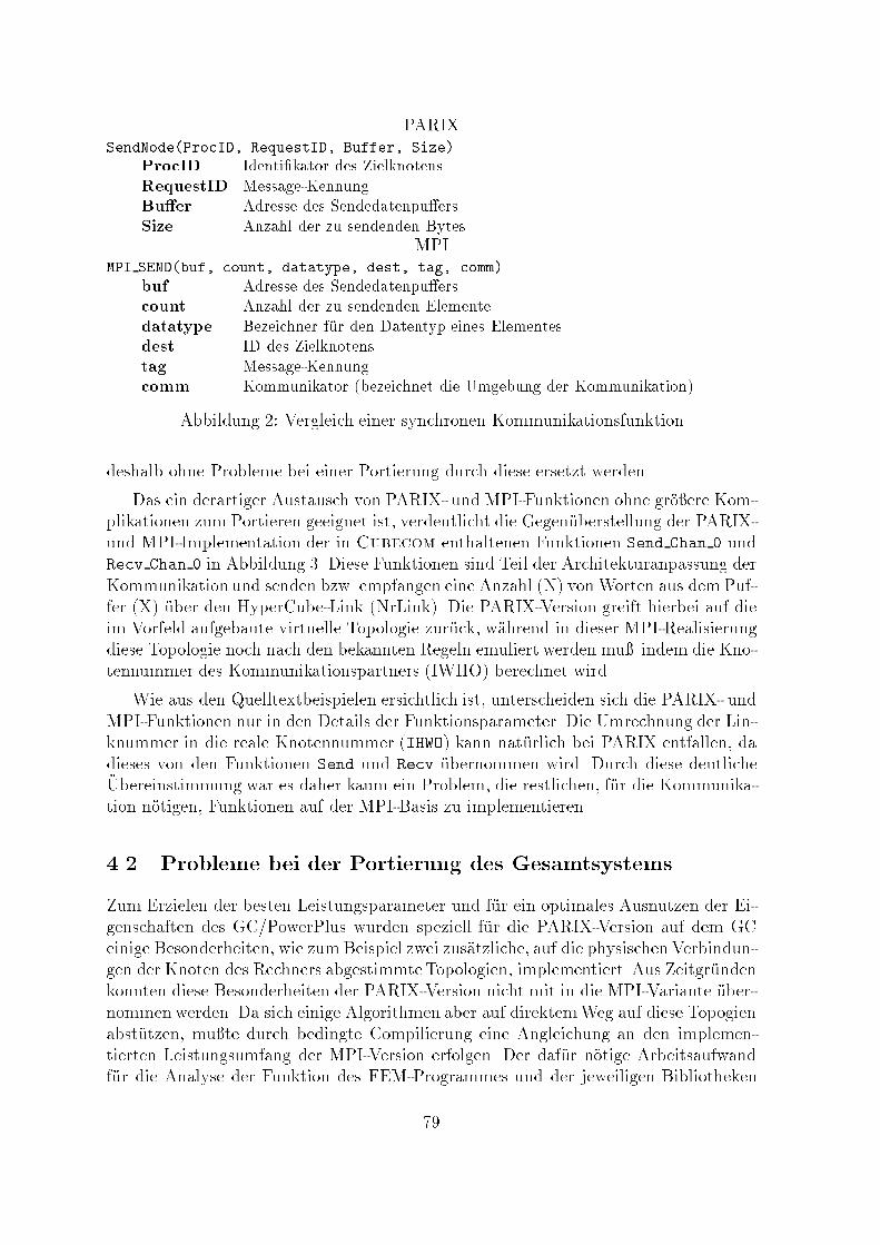
PARIXSendNode(ProcID, RequestID, Buffer, Size)ProcID Identi�kator des ZielknotensRequestID Message-KennungBu�er Adresse des Sendedatenpu�ersSize Anzahl der zu sendenden BytesMPIMPI SEND(buf, count, datatype, dest, tag, comm)buf Adresse des Sendedatenpu�erscount Anzahl der zu sendenden Elementedatatype Bezeichner f�ur den Datentyp eines Elementesdest ID des Zielknotenstag Message-Kennungcomm Kommunikator (bezeichnet die Umgebung der Kommunikation)Abbildung 2: Vergleich einer synchronen Kommunikationsfunktiondeshalb ohne Probleme bei einer Portierung durch diese ersetzt werden.Das ein derartiger Austausch von PARIX- und MPI-Funktionen ohne gr�o�ere Kom-plikationen zum Portieren geeignet ist, verdeutlicht die Gegen�uberstellung der PARIX-und MPI-Implementation der in Cubecom enthaltenen Funktionen Send Chan 0 undRecv Chan 0 in Abbildung 3. Diese Funktionen sind Teil der Architekturanpassung derKommunikation und senden bzw. empfangen eine Anzahl (N) von Worten aus dem Puf-fer (X) �uber den HyperCube-Link (NrLink). Die PARIX-Version greift hierbei auf dieim Vorfeld aufgebaute virtuelle Topologie zur�uck, w�ahrend in dieser MPI-Realisierungdiese Topologie noch nach den bekannten Regeln emuliert werden mu� indem die Kno-tennummer des Kommunikationspartners (IWHO) berechnet wird.Wie aus den Quelltextbeispielen ersichtlich ist, unterscheiden sich die PARIX- undMPI-Funktionen nur in den Details der Funktionsparameter. Die Umrechnung der Lin-knummer in die reale Knotennummer (IHWO) kann nat�urlich bei PARIX entfallen, dadieses von den Funktionen Send und Recv �ubernommen wird. Durch diese deutliche�Ubereinstimmung war es daher kaum ein Problem, die restlichen, f�ur die Kommunika-tion n�otigen, Funktionen auf der MPI-Basis zu implementieren.4.2 Probleme bei der Portierung des GesamtsystemsZum Erzielen der besten Leistungsparameter und f�ur ein optimales Ausnutzen der Ei-genschaften des GC/PowerPlus wurden speziell f�ur die PARIX-Version auf dem GCeinige Besonderheiten, wie zumBeispiel zwei zus�atzliche, auf die physischen Verbindun-gen der Knoten des Rechners abgestimmteTopologien, implementiert. Aus Zeitgr�undenkonnten diese Besonderheiten der PARIX-Version nicht mit in die MPI-Variante �uber-nommen werden. Da sich einige Algorithmen aber auf direktemWeg auf diese Topogienabst�utzen, mu�te durch bedingte Compilierung eine Angleichung an den implemen-tierten Leistungsumfang der MPI-Version erfolgen. Der daf�ur n�otige Arbeitsaufwandf�ur die Analyse der Funktion des FEM-Programmes und der jeweiligen Bibliotheken79

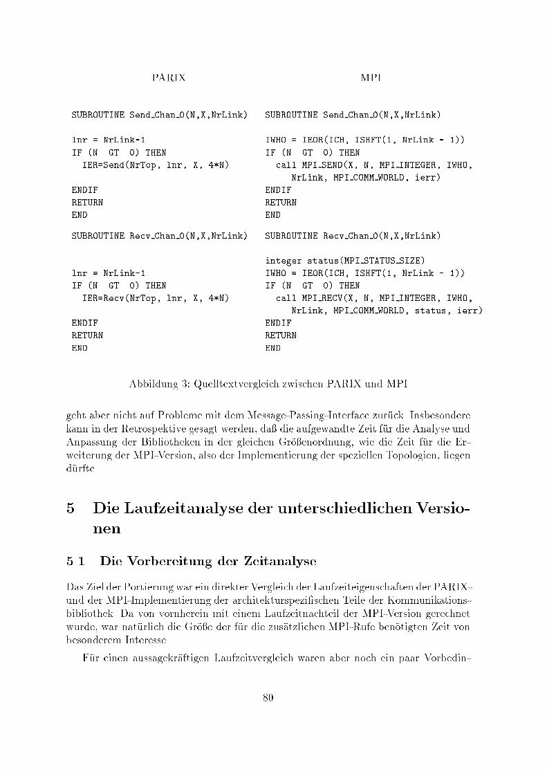
PARIX MPISUBROUTINE Send Chan 0(N,X,NrLink) SUBROUTINE Send Chan 0(N,X,NrLink)... ...lnr = NrLink-1 IWHO = IEOR(ICH, ISHFT(1, NrLink - 1))IF (N .GT. 0) THEN IF (N .GT. 0) THENIER=Send(NrTop, lnr, X, 4*N) call MPI SEND(X, N, MPI INTEGER, IWHO,NrLink, MPI COMM WORLD, ierr)ENDIF ENDIFRETURN RETURNEND ENDSUBROUTINE Recv Chan 0(N,X,NrLink) SUBROUTINE Recv Chan 0(N,X,NrLink)... ...integer status(MPI STATUS SIZE)lnr = NrLink-1 IWHO = IEOR(ICH, ISHFT(1, NrLink - 1))IF (N .GT. 0) THEN IF (N .GT. 0) THENIER=Recv(NrTop, lnr, X, 4*N) call MPI RECV(X, N, MPI INTEGER, IWHO,NrLink, MPI COMM WORLD, status, ierr)ENDIF ENDIFRETURN RETURNEND ENDAbbildung 3: Quelltextvergleich zwischen PARIX und MPIgeht aber nicht auf Probleme mit dem Message-Passing-Interface zur�uck. Insbesonderekann in der Retrospektive gesagt werden, da� die aufgewandte Zeit f�ur die Analyse undAnpassung der Bibliotheken in der gleichen Gr�o�enordnung, wie die Zeit f�ur die Er-weiterung der MPI-Version, also der Implementierung der speziellen Topologien, liegend�urfte.5 Die Laufzeitanalyse der unterschiedlichen Versio-nen5.1 Die Vorbereitung der ZeitanalyseDas Ziel der Portierung war ein direkter Vergleich der Laufzeiteigenschaften der PARIX-und der MPI-Implementierung der architekturspezi�schen Teile der Kommunikations-bibliothek. Da von vornherein mit einem Laufzeitnachteil der MPI-Version gerechnetwurde, war nat�urlich die Gr�o�e der f�ur die zus�atzlichen MPI-Rufe ben�otigten Zeit vonbesonderem Interesse.F�ur einen aussagekr�aftigen Laufzeitvergleich waren aber noch ein paar Vorbedin-80

gungen zu scha�en. Durch den Verzicht auf die architekturoptimierten virtuellen To-pologien bei der Implementierung der MPI-Version hat nat�urlich diese Variante eindeutliches Manko aufzuweisen. Um relevante Aussagen zu gew�ahrleisten, wurde des-halb eine weitere Version erstellt, welche auf die PARIX-Umgebung des GC/PowerPluszugreift, aber wie die MPI-Version nicht f�ur dessen Architektur besonders optimiertwurde.Es folgt eine �Ubersicht �uber die erstellten, bzw. verwendeten Implementationen derarchitekturabh�angigen Kommunikationsfunktionen mit deren Leistungsmerkmalen:ppc arbeitet mit der orginalen, f�ur den GC/PowerPlus optimiertenPARIX-Version der Bibliothek Cubecom mit drei, zum Teil an diephysische Linkstruktur des Rechners angepa�ten, virtuellen Topologi-en (HyperCube, Ring und KettAkk)ppcblank basiert auf einer abger�usteten PARIX-Variante der Kommunika-tionsbibliothek Cubecom ohne spezielle Optimierungen f�ur denGC/PowerPlus und hat damit den gleichen Aufbau und die gleichenVoraussetzungen wie die MPI-Version ppcmpippcmpi nutzt f�ur die Kommunikation die grundlegenden, synchronen Funk-tionen der MPI-Bibliothek; die f�ur die Arbeit des Programmes n�otigeHyperCube-Topologie wird durch Emulation bereitgestellt; spezielleAnpassungen an die Kommunikationsstruktur des Rechners werdennicht vorgenommenAus den nun m�oglichen Laufzeitvergleichen k�onnen damit zwei Aussagen gebildetwerden:� Der Geschwindigkeitsgewinn durch die Anpassung und Optimierung eines PARIX-Programmes an die spezielle Linkstruktur der zugrundeliegenden Architektur, alsDi�erenz der Laufzeiten der Versionen ppc und ppcblank.� Der Laufzeitoverhead, den die abstrahierende \Zwischenschicht" MPI mit sichbringt und mit dem die Vorteile der Architekturunabh�angigkeit erkauft werdenm�ussen. Ablesbar ist dies aus der Laufzeitdi�erenz der Varianten ppcmpi undppcblank.5.2 Die ZeitanalyseGemessen wurden die folgenden Laufzeiten des FEM-Programmes mit der internenZeitmessung dieser Applikation, die sowohl die Zeit f�ur die Kommunikation, als auchf�ur die Berechnung mit einbezieht. Ermittelt wurden der Zeitverbrauch der drei vorge-stellten Versionen bei zunehmender Verfeinerung des Problems. Ein Ma� f�ur die stei-gende Komplexit�at und den wachsenden Aufwand ist der Parameter Level. Ausgehendvon einer Grundau �osung des Problems bei Level 1, wird mit steigender Au �osung die81

Kantenl�ange der �niten Elemente halbiert. Damit vervierfacht sich bei jedem Level-Schritt die Anzahl der �niten Elemente. Entsprechend dazu steigt der Berechnungs-,Speicher- und Kommunikationsaufwand des Problems.Gearbeitet wurde auf dem GC/PowerPlus-128 mit einem Cluster aus acht Proze-soren. Berechnet wurde hierbei das Problem \q". Die PARIX-Versionen wurden direktauf den Knoten durch px run ... gestartet. Die MPI-Variante ben�otigt f�ur den Startdas Programm mpirun, welches den Code der Applikation l�ad und dessen Ausf�uhrungauf den einzelnen Knoten einleitet.Hier folgt eine Aufstellung der ermittelten Zeiten (in Sekunden) in tabellarischerund graphischer Form (Abbildung 4) in Abh�angigkeit von dem Au �osunglevel desProblems: Level 1 2 3 4 5 6ppc 0,27 0,30 0,44 0,79 2,19 7,31ppcblank 0,24 0,29 0,40 1,90 3,22 8,60ppcmpi 0,28 0,30 0,45 1,83 3,42 8,75ppcmpi ppcblank ppc

Level

Zeit/s

1 2 3 4 5 6

0

2

4

6

8

10

Abbildung 4: Die Laufzeit bei den einzelnen Versionen der KommunikationsbibliothekDie dargestellten Zeiten sind die Werte einer Me�reihe, die unter den beschriebenenBedingungen aufgenommen wurde. Sie steht exemplarisch f�ur alle durchgef�uhrten Zeit-messungen, die auch mit anderen Clustergr�o�en und Problemen durchgef�uhrt wurden.Gr�o�ere Streuungen der Bearbeitungszeiten konnten bei gleichbleibenden Bedingungen(Clustergr�o�e, Problem) nicht festgestellt werden. Auch bei ver�anderten Einstellungen82

behielten die Berechnungszeiten ihre Relationen bei, so da� die angegebene Me�reiheals representativ f�ur das Zeitverhalten der Applikation angesehen werden kann.5.3 Resultat der ZeitanalyseWie besonders aus der Gra�k zu entnehmen ist, wird durch die Architekturoptimie-rung in der PARIX-Implementation (ppc) eine deutliche Laufzeitverbesserung ge-gen�uber einer konventionellen PARIX-Applikation erreicht. Der Laufzeitoverhead derMPI-Bibliothek ist dagegen gering. Dies erkl�art sich aus der Gleichheit der Funktiona-lit�at der benutzten PARIX- oder MPI-Routinen. Die Prozeduren der MPI-Bibliothekmu�ten lediglich die Kommunikationsrufe und deren Parameter an die entsprechendenPARIX-Funktionen weiterleiten.6 Die m�oglichen Verbesserungen der MPI-VersionWie aus dem eben genannten Resultaten hervorgeht, ist als entscheidendes Kriteriumf�ur die Laufzeit die Anpassung an die Architektur und Kommunikationsstruktur zusehen. Die Performance der MPI-Implementation k�onnte also noch dadurch gesteigertwerden, da� analog zu der orginalen PARIX-Variante, spezielle und angepa�te virtu-elle Topologien implementiert werden. Diese w�urden die Struktur des GC/PowerPlusausnutzen und damit die Kommunikationswege und -entfernungen optimieren und dieKommunikation gleichm�a�iger im Netz der Links verteilen. Eine solche, optimierteVariante k�ame mit hoher Wahrscheinlichkeit an die Leistungsf�ahigkeit der PARIX-Variante heran, bringt aber auch gleichzeitig den Nachteil der Architekturabh�angigkeitmit sich.Die bisherige Implementation der MPI-Variante ist in Anlehnung an Abbildung 1als eigenst�andiger Teil der Bibliothek Cubecom zu sehen. Hierbei hat er den Vorteil,da� er nicht nur als Bindeglied der allgemeinen Funktionen zum GC/PowerPlus, son-dern auch zu einer Vielzahl von anderen Parallelrechnern oder Workstation-Clusternfungieren kann. Trotzdem werden viele besondere M�oglichkeiten des Message-Passing-Interface-Standards nicht verwendet. So werden s�amtliche komplexeren Kommunika-tionsfunktionen, wie zum Beispiel Funktionen f�ur globale Kommunikation oder auchf�ur den simultanen Austausch von Werten zwischen zwei Knoten von der BibliothekCubecom realisiert. All diese Aufgaben k�onnte allerdings auch die MPI-Bibliothek�ubernehmen und auf direkterem Wege auf die Hardware umsetzen. Die gr�o�ere Lei-stungsf�ahigkeit von MPI w�urde durch eine Umstrukturierung der Kommunikationsbi-bliothek nach folgendem Schema (Abbildung 5) erschlossen werden.Hierbei �ubernimmt MPI weite Teile der komplexen Kommunikationsfunktionenund die Anpassung an die jeweilige Parallelrechnerarchitektur. Vom Entwickler derApplikationen oder der Bibliotheken ist kein architekturspezi�scher Code mehr zuschreiben, sondern die Bibliothek Cubecom lediglich mit der entsprechenden MPI-Implementation zu linken. 83

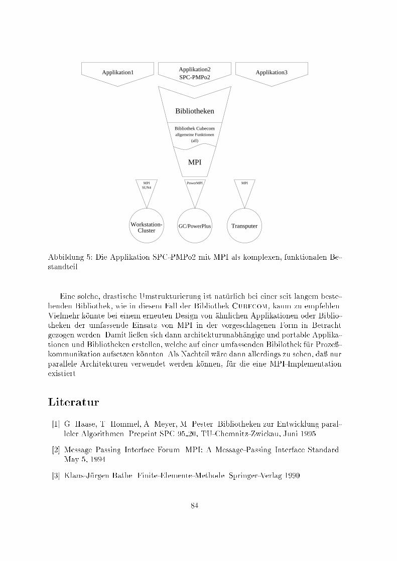
Applikation1 Applikation2SPC-PMPo2

Applikation3

Bibliotheken

Bibliothek Cubecomallgemeine Funktionen

(all)

MPI

Workstation- TransputerCluster

MPI PowerMPI MPISUN4

GC/PowerPlusAbbildung 5: Die Applikation SPC-PMPo2 mit MPI als komplexen, funktionalen Be-standteilEine solche, drastische Umstrukturierung ist nat�urlich bei einer seit langem beste-henden Bibliothek, wie in diesem Fall der Bibliothek Cubecom, kaum zu empfehlen.Vielmehr k�onnte bei einem erneuten Design von �ahnlichen Applikationen oder Biblio-theken der umfassende Einsatz von MPI in der vorgeschlagenen Form in Betrachtgezogen werden. Damit lie�en sich dann architekturunabh�angige und portable Applika-tionen und Bibliotheken erstellen, welche auf einer umfassenden Bibilothek f�ur Proze�-kommunikation aufsetzen k�onnten. Als Nachteil w�are dann allerdings zu sehen, da� nurparallele Architekturen verwendet werden k�onnen, f�ur die eine MPI-Implementationexistiert.Literatur[1] G. Haase, T. Hommel, A. Meyer, M. Pester. Bibliotheken zur Entwicklung paral-leler Algorithmen. Preprint SPC 95 20, TU-Chemnitz-Zwickau, Juni 1995[2] Message Passing Interface Forum. MPI: A Message-Passing Interface Standard.May 5, 1994[3] Klaus-J�urgen Bathe. Finite-Elemente-Methode. Springer-Verlag 199084

Application Oriented MonitoringMatthias Ohlenrothmoh@informatik.tu-chemnitz.dehttp://noah.informatik.tu-chemnitz.de/members/ohlenroth/ohlenroth.htmlAbstractOptimizing parallel applications is a complex task. Special tools are requiredto record and analyze their behaviour. This paper introduces facilities o�ered bymonitoring environments based on source code instrumentation. Typical com-ponents of monitoring environments and their use are explained. Time basedand event based trace generation are introduced. A sample monitoring sessionillustrates possibilities and limitations of available tools.

85

1 IntroductionMonitoring becomes more and more important, especially for parallel computing envi-ronments. E�cient parallel programming is a di�cult task. The application program-mer has to select the underlying services carefully for optimal speedup. This processis in uenced by interactions and dependencies between all software and hardware lay-ers. Potential performance problems must be detected while testing the application.Monitoring tools provide mechanisms to accelerate this task. Usually the programmerinserts probe functions into the source code. This requires several loops of the form:add probe function { execute application { analyze data.Portability becomes more and more important for parallel applications. But opti-mal performance requires precise adaption to the underlying parallel computer. Soft-ware abstractions are used to tone down this contrast. One sample is the messagepassing library MPI. The interface de�nition permits e�cient implementation for dif-ferent parallel computers. Interactions between application, message passing libraryand hardware have great impact on the performance of the application. One abstrac-tion layer may o�er di�erent ways to solve a particular implementation problem. Thechoice made by the programmer in uences the performace of the application.Performance tuning of sequential applications requires analyzation of runtime dataand interactions with lower layers of the architecture. Pro�ler help to �nd often calledor long running functions. It is likely that optimizing these functions reduces theexecution time considerably. Interactions between application and operating systemmay be analyzed. Special tools allow one to trace system calls.Tuning parallel applications is more complex. A parallel program consists of com-municating processes or threads. The e�ciency depends on the algorithm, the im-plementation, the system software and the hardware. Performance bottlenecks re-sult from insu�cient parallel workload, communication and synchronization problems.Monitoring environments trace program behaviour, especially synchronization, com-munication, blocking times and application speci�c events. Ine�cient program regionscan be identi�ed from application traces. Changes will be made to ensure high localityof computation, equal workload distribution and e�cient communication.2 The Components of a Monitoring EnvironmentA monitoring environment consists of an instrumentation tool11, a trace library anda visualization tool. These components correspond to the three tasks of a monitoringsession:� instrument the application,11Some systems do not o�er an instrumentation tool. Other solutions integrate compiler and in-strumentation tool. 86

� execute the application,� analyze the trace data.The instrumented application generates trace data during execution. These datacan be examined on-line or o�-line. O�-line tools are independent from the programexecution. Stored trace data can be analyzed as time permits. On-line tools o�erperformance pictures of running applications. Special connections transfer trace databetween application and presentation tool. Backward connections permit steering ofthe application. The user may in uence the data partitioning of the application forinstance. Figure 1 illustrates both approaches.Source Code

Instrumen−tation Tool Compiler

Application

Monitoring Library

Trace File

Off−line Monitoring

Source Code

Instrumen−tation Tool Compiler

On−line Monitoring

Presentation Tool

Application

Monitoring Library

Presentation ToolFigure 1: Monitoring Environments.2.1 The InstrumentationThe instrumentation step adds calls to probe functions to the application code. Thiscan be done automatically by the compiler. Automatic instrumentation is limited toprogram structures which are visible to the compiler. Other tools modify the programsource code directly. After parsing the �le instrumentation can be done interactivelyby the programmer. Tools permit the instrumentation of function calls and loops.The following example demonstrates the instrumentation of a procedure call. Probefunctions are inserted before and after the function test func()....#define EventID 1000;probe function(EventID);test function();probe function(EventID); 87

...The �rst probe function starts an interval timer inside the trace library. The secondcall stops this timer and generates a trace record containing the following members:� node number,� event identi�er,� value of the event local counter,� local time,� time duration.The node number identi�es the thread or process of the parallel application. Eachevent is represented by its unique event identi�er. The number of occurrences of anevent is recorded by the library. The local time and the duration of the event arestored.Speci�c instrumentation may be added manually. To this class belong applicationdependent events and time duration events without relation to program structure.Timer might be started in one function and stopped inside a di�erent function.The instrumented source code will be saved to a new �le. This �le must be compiledand linked with the application instead of the original one. Direct instrumentation ofsource code does not require modi�cations of the compilation system.2.2 The Trace LibraryThe trace library contains the probe functions and other code required to manage tracedata streams. The library collects trace data, saves them to a trace �le or forwardsthem to on-line visualization tools. The management of trace data requires resources ofthe application. These are processing time and memory. Event records will be bu�eredby the library. Some libraries use their own thread of execution.Trace libraries require di�erent levels of initialization. Some libraries are self-initializing. Default parameters like trace �le name or socket number can be over-written by the application. Special care is needed during application shutdown. Thetrace data bu�er must be ushed before the main function of the application returns.This requires insertion of an explicit call to the trace library. Instrumentation toolsgenerate appropriate wrapper functions for the main function. The wrapper functionperforms the required actions. 88

2.3 The Trace FileThe trace �le contains records for all events processed by the monitoring library. De-pending on the monitoring environment one application trace consists of one or severaldi�erent trace �les. Every node may generate its own �le. These �les have to bemerged into one �le before analyzing the trace. Merging tools order records by theirtime stamp. Users may specify other rules.Although some of the �le format speci�cations are published most of the monitoringenvironments use their own �le format. This prevents one from using a visualizationtool with trace data generated by a di�erent environment. Reasons for new �le formatsare limitations of other speci�cations. One known format is the self de�ning dataformat (SDDF) used by the Pablo [RAM+92] performance analysis environment. The�le contains information about the used records followed by the data records. ASCIIand binary representations of the same speci�cation are de�ned. A set of tools performtransformations between both representations. Binary �les with di�erent byte orderingcan be transformed to the native byte ordering of the host computer. Trace datagenerated on a parallel machine may be analyzed on a host system with di�erentarchitecture.2.4 The Visualization ToolThe presentation tool provides a framework for trace data processing and visualization.Some tools can be con�gured by the user. Programs for on-line and o�-line visualizationare available.A visualization session consists of module instances and connections between them.Con�gurable tools o�er a set of modules. The user selects modules from the groups�le I/O, �ltering, data processing and visualization. Modules and connections form anacyclic graph. Connections transfer data records between modules. Di�erent recordsmay be passed along one connection. Modules have to be con�gured. This includesinput ports, output ports and internal parameters. Sessions may be saved and reusedlater.Figuring out performance problems is a di�cult process. Several modi�cation of thesession con�guration are required to clarify the problem. Hence the following procedurehas to be performed several times:create or modify session con�guration#process trace data and generate graphical presentation#interpret dataThe user has to analyze visualized data and �gure out the performance problem.89

Some tools o�er di�erent levels of support. New users may bene�t from prede�nedsession con�gurations. More experienced users want to create their own sessions. Ex-pert users may reach limits of the modules provided by the program. They wish tocreate new modules and extend the visualization tool. The Pablo [RAM+92] tool o�ersa class library. The library separates module implementation, connection managementand low-level data processing. New modules can be build on top of the existing classlibrary.On-line visualization tools contain components for on-line program steering. Ad-justments made by the user are propagated back to the monitoring library. Specialvariables transfer information back to the application. The application de�nes thesevariables and registers them with the monitoring library.3 Trace Data GenerationThis section introduces di�erent approaches to generate trace data. Each peace of atrace �le, called record, provides information about one particular event of the applica-tion. This information is limited to one thread or processing node and does not re ectglobal states. A record represents an application event. All records together provideinformation about the behaviour of the application.Architecture support for monitoring di�ers. Some architectures provide hardwaresupport for trace data generation. Depending on the level of hardware support hard-ware monitoring or hybrid monitoring may be used. Hybrid monitoring combines hard-ware and software facilities to produce accurate trace information. Software monitoringis used on systems without hardware support. Two common monitoring techniques are� time-driven monitoring and� event-driven monitoring.Both approaches provide di�erent levels of details, program perturbation and imple-mentation costs.3.1 Time-driven MonitoringTime-driven monitoring requires operating system support. The program counter issampled periodically by the operating system. Sampling is local to each thread orprocessing node. This technique exposes the most expensive parts of the application.It is likely that most samples belong to often called or long-running functions. Theprocessing of program counter samples requires compiler support. Samples must be as-signed to source code lines or functions. The sampling frequency used by the operatingsystem has great impact on the accuracy. 90

3.2 Event-driven MonitoringA chain of events represents the program behaviour. The level of precision is ad-justable. Event-driven monitoring requires higher implementation cost. The program-mer is concerned with the instrumentation process directly. Special instrumentationrequires coding by hand. This method o�ers more control to the programmer. Hechoses relevant events and controls directly the level of precision. Events are generatedby calls to the monitoring library. Each call to a probe function requires processingtime and delays program execution. The library bu�ers event records and writes themto the trace �le. One major disadvantage is the program perturbation. Libraries likePablo provide mechanisms to enable or disable probe functions and ajust the eventtype on-line.The following event types are distinguished:� Trace event,� Count event,� Time event.Trace events represent single program events, i.e. function calls. Application spe-ci�c events belong to this class. Each event record contains at least the local time,the event identi�er and the node number. The application may append further data.A sample code fragment is given in �gure 2. All calls to the function doit() aretraced. Count events register the number of occurences of particular events. The mon-itoring library appends the event number automatically. The use of count events isdemonstrated by function start(). Time events are used to measure the time dura-tion between two application-speci�c instrumentation points. The monitoring librarymanages one interval timer for each time event. The timer is started and stopped bytwo consecutive events. Time events are used to measure the time between calls to thefunctions start() and stop() of example 2. The same event would be generated ifboth functions are called in reverse order.start () fcount event ( COUNT EVENT 1 );time event ( TIME EVENT 1 );...gstop () ftime event ( TIME EVENT 1 );...g 91

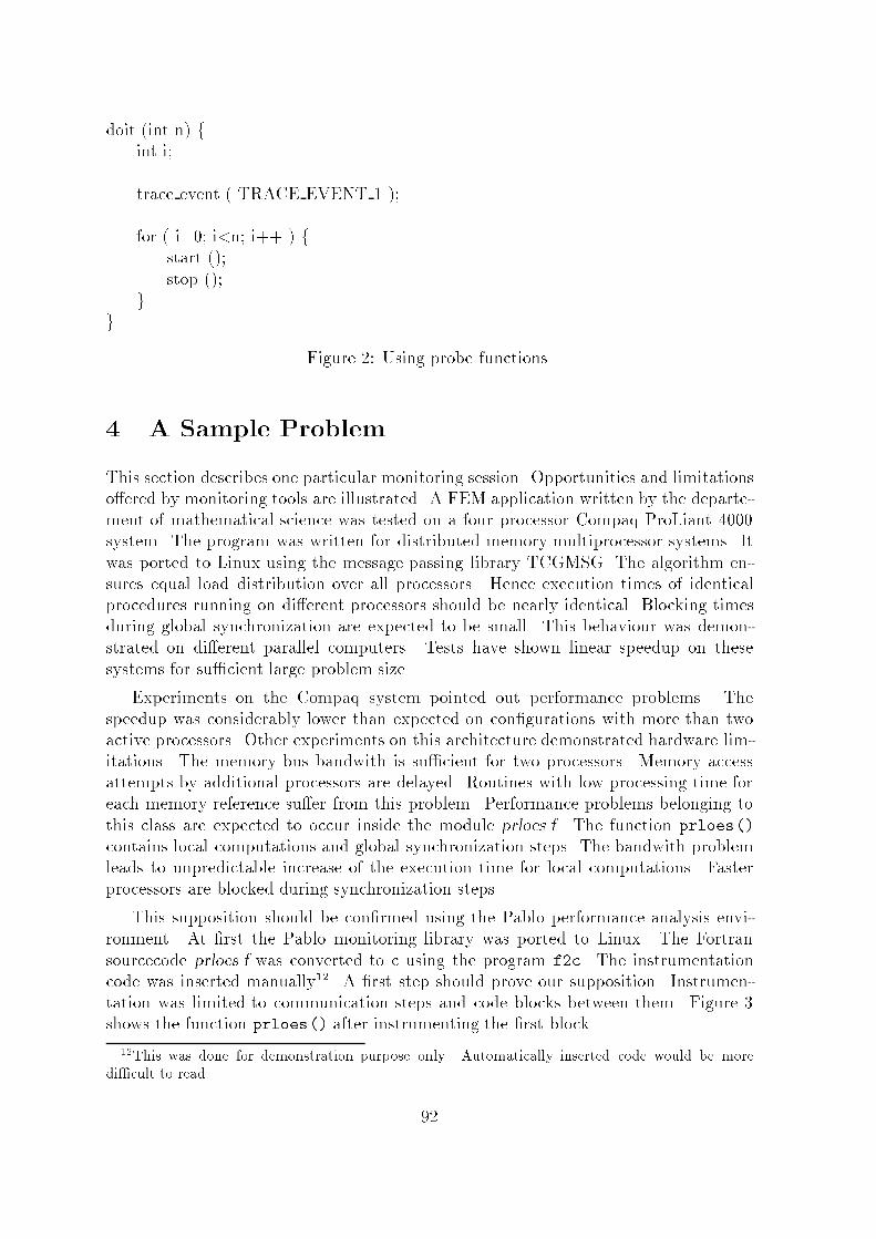
doit (int n) fint i;trace event ( TRACE EVENT 1 );for ( i=0; i<n; i++ ) fstart ();stop ();gg Figure 2: Using probe functions.4 A Sample ProblemThis section describes one particular monitoring session. Opportunities and limitationso�ered by monitoring tools are illustrated. A FEM application written by the departe-ment of mathematical science was tested on a four processor Compaq ProLiant 4000system. The program was written for distributed memory multiprocessor systems. Itwas ported to Linux using the message passing library TCGMSG. The algorithm en-sures equal load distribution over all processors. Hence execution times of identicalprocedures running on di�erent processors should be nearly identical. Blocking timesduring global synchronization are expected to be small. This behaviour was demon-strated on di�erent parallel computers. Tests have shown linear speedup on thesesystems for su�cient large problem size.Experiments on the Compaq system pointed out performance problems. Thespeedup was considerably lower than expected on con�gurations with more than twoactive processors. Other experiments on this architecture demonstrated hardware lim-itations. The memory bus bandwith is su�cient for two processors. Memory accessattempts by additional processors are delayed. Routines with low processing time foreach memory reference su�er from this problem. Performance problems belonging tothis class are expected to occur inside the module prloes.f. The function prloes()contains local computations and global synchronization steps. The bandwith problemleads to unpredictable increase of the execution time for local computations. Fasterprocessors are blocked during synchronization steps.This supposition should be con�rmed using the Pablo performance analysis envi-ronment. At �rst the Pablo monitoring library was ported to Linux. The Fortransourcecode prloes.f was converted to c using the program f2c. The instrumentationcode was inserted manually12. A �rst step should prove our supposition. Instrumen-tation was limited to communication steps and code blocks between them. Figure 3shows the function prloes() after instrumenting the �rst block.12This was done for demonstration purpose only. Automatically inserted code would be moredi�cult to read. 92

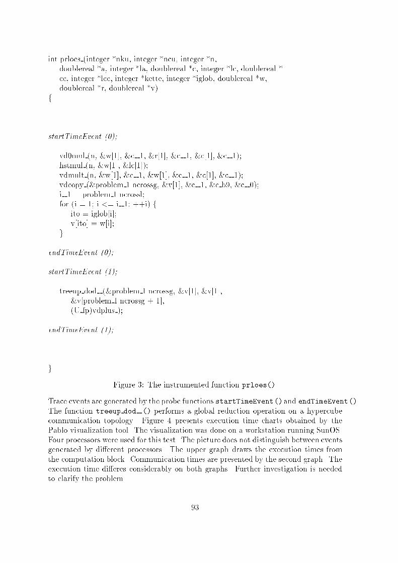
int prloes (integer *nku, integer *ncu, integer *n,doublereal *a, integer *la, doublereal *c, integer *lc, doublereal *cc, integer *lcc, integer *kette, integer *iglob, doublereal *w,doublereal *r, doublereal *v)f...startTimeEvent (0);vd0mul (n, &w[1], &c 1, &r[1], &c 1, &c[1], &c 1);hstmul (n, &w[1], &lc[1]);vdmult (n, &w[1], &c 1, &w[1], &c 1, &c[1], &c 1);vdcopy (&problem 1.ncrossg, &v[1], &c 1, &c b9, &c 0);i 1 = problem 1.ncrossl;for (i = 1; i <= i 1; ++i) fito = iglob[i];v[ito] = w[i];gendTimeEvent (0);startTimeEvent (1);treeup dod (&problem 1.ncrossg, &v[1], &v[1],&v[problem 1.ncrossg + 1],(U fp)vdplus );endTimeEvent (1);....g Figure 3: The instrumented function prloes().Trace events are generated by the probe functions startTimeEvent()and endTimeEvent().The function treeup dod () performs a global reduction operation on a hypercubecommunication topology. Figure 4 presents execution time charts obtained by thePablo visualization tool. The visualization was done on a workstation running SunOS.Four processors were used for this test. The picture does not distinguish between eventsgenerated by di�erent processors. The upper graph draws the execution times fromthe computation block. Communication times are presented by the second graph. Theexecution time di�eres considerably on both graphs. Further investigation is neededto clarify the problem. 93

Figure 4: Execution and communication time.The traced code block contains four function calls. During a second step thesefunctions are instrumented separately. Figure 5 lists the instrumented code. Procedureentry and exit events are generated by the function PabloTraceProc(). A uniqueidenti�er is assigned to each event. Figure 6 presents the obtained trace data. Eachgraph shows the execution time of one function called by prloes(). The �rst graphbelongs to function vd0mul (). Other functions are ordered as they occure in the sourcecode. The execution time of the functions vd0mul () and treeup dod () di�eresconsiderably. Both functions contribute to the performance problem. We evaluate thefunction vd0mul () in detail. Figure 7 lists the source code. Memory operations are94

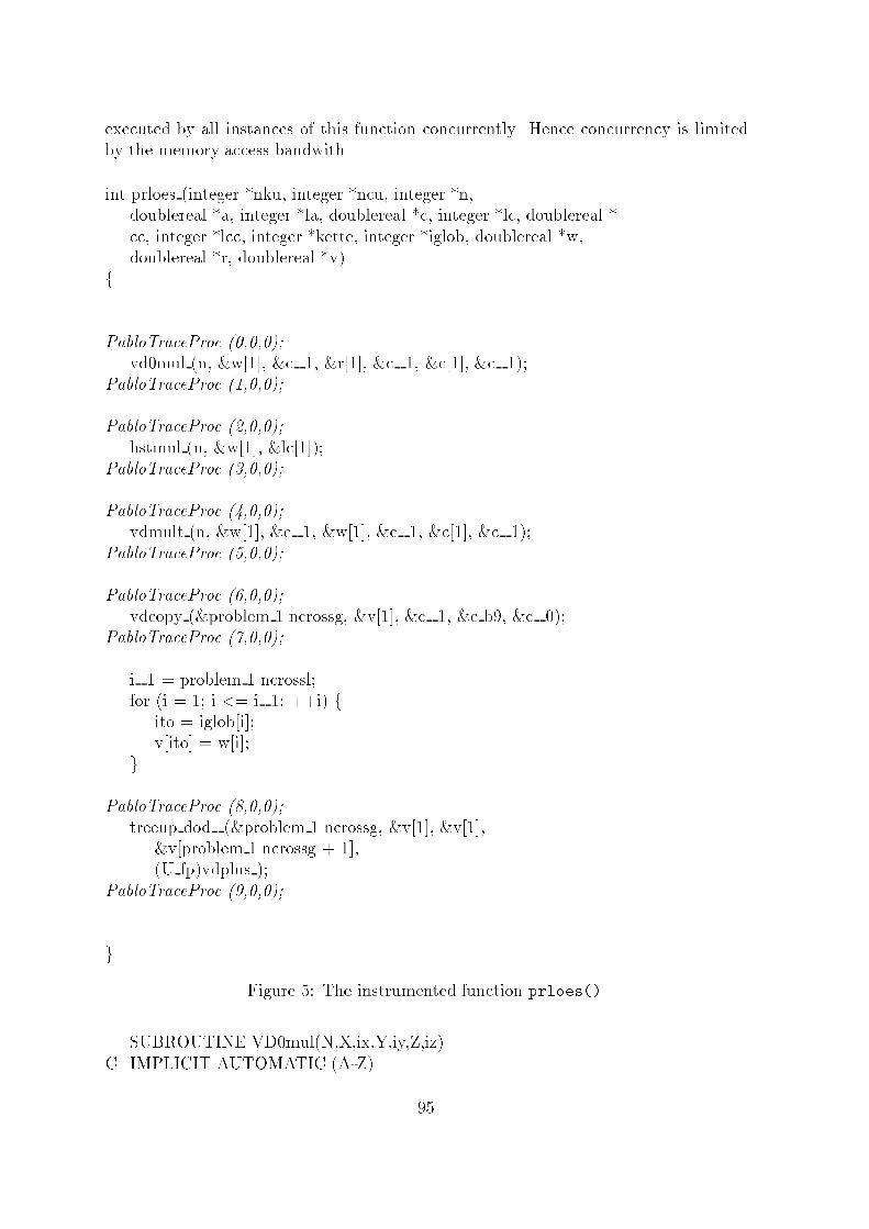
executed by all instances of this function concurrently. Hence concurrency is limitedby the memory access bandwith.int prloes (integer *nku, integer *ncu, integer *n,doublereal *a, integer *la, doublereal *c, integer *lc, doublereal *cc, integer *lcc, integer *kette, integer *iglob, doublereal *w,doublereal *r, doublereal *v)f...PabloTraceProc (0,0,0);vd0mul (n, &w[1], &c 1, &r[1], &c 1, &c[1], &c 1);PabloTraceProc (1,0,0);PabloTraceProc (2,0,0);hstmul (n, &w[1], &lc[1]);PabloTraceProc (3,0,0);PabloTraceProc (4,0,0);vdmult (n, &w[1], &c 1, &w[1], &c 1, &c[1], &c 1);PabloTraceProc (5,0,0);PabloTraceProc (6,0,0);vdcopy (&problem 1.ncrossg, &v[1], &c 1, &c b9, &c 0);PabloTraceProc (7,0,0);i 1 = problem 1.ncrossl;for (i = 1; i <= i 1; ++i) fito = iglob[i];v[ito] = w[i];gPabloTraceProc (8,0,0);treeup dod (&problem 1.ncrossg, &v[1], &v[1],&v[problem 1.ncrossg + 1],(U fp)vdplus );PabloTraceProc (9,0,0);....g Figure 5: The instrumented function prloes().SUBROUTINE VD0mul(N,X,ix,Y,iy,Z,iz)C IMPLICIT AUTOMATIC (A-Z) 95

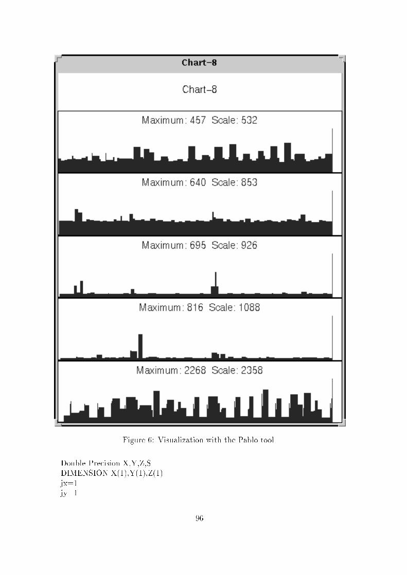
Figure 6: Visualization with the Pablo tool.Double Precision X,Y,Z,SDIMENSION X(1),Y(1),Z(1)jx=1jy=1 96

jz=1DO 1 I=1,NS = Y(jy)IF (Z(jz) .EQ. 0D0) S=0D0X(jx) = Sjx = jx + ixjy = jy + iy1 jz = jz + izRETURNEND Figure 7: The function VD0mul ().Althrough monitoring helps to identify the performanc problem it does not providea solution. The presented problem cannot be solved due to hardware limitations. Asecond dependency was not mentioned until now. The past tests were done using smallFEM problems. Each processor has to perform computations on small memory regions.Only some cache lines must be loaded by each processor. Larger problems require alot of load operations. In this case the average load delay would be identical on allprocessors. Hence the problem would be invisible to monitoring atempts.The sample described above illustrates some issues which may limit the success ofmonitoring sessions:� The visability of problems may be limited.� The visability of problems depends on input data.� Execution time variations are hidden after several local iterations.5 ConclusionsMonitoring environments provide tools for performance analysis of parallel applications.A source code based method which does not require compiler support was introduced.User controlled instrumentation o�ers high exibility. Monitoring libraries generateand save event records. Instrumentation should be done carefully. Monitoring activitiesrequire application resources and perturb the application. Hence application behaviourmay change.Capabilities and limitation of monitoring tools were demonstrated using a sampleproblem. A small set of probe functions is su�cient for most monitoring requirements.Expressive and con�gurable graphical tools ease interpretation of trace data. Thisrequires exible �ltering and processing capabilities.Future work adresses the topics visualization, event processing and operating sys-tem monitoring. Visualization and processing facilities o�ered by di�erent tools will be97

analyzed in detail. Knowledge how current tools satis�es the need of programmers isneeded to prepare better tools. While preparing the demonstration some experimentshave shown transient e�ects. These e�ects are attributed to operating system activi-ties. Identifying them requires monitoring facilities inside the operating system. Thisincludes interrupt processing, scheduling and other process state switches. We want tointegrate monitoring facilities into Linux/SMP.References[GEKS94] W. Gu, G. Eisenhauer, E. Kraemer, and K. Schwan, Falcon: On-line Moni-toring and Steering of Large-Scale Parallel Programs, Tech. report, Collegeof Computing, Georgia Institute of Technology, Atlanta, Georgia, 1994,URL: ftp://ftp.cc.gatech.edu/pub/tech-reports/1994/GIT-CC-94-21.ps.Z.[GVS94] W. Gu, J. Vetter, and K. Schwan, An Annotated Bibliographyof Interactive Program Steering, Tech. report, College of Comput-ing, Georgia Institute of Technology, Atlanta, Georgia, 1994, URL:ftp://ftp.cc.gatech.edu/pub/tech-reports/1994/GIT-CC-94-15.ps.Z.[Noe94] R. J. Noe, Pablo Instrumentation Environment Reference Manual, Tech.report, Department of Computer Science, University of Illinois, Illinois,1994.[RAM+92] D. A. Reed, R. A. Aydt, T. M. Madhyastha, R. J. Noe, K. A. Shields, andB. W. Schwartz, An Overview of the Pablo Performance Analysis Environ-ment, Tech. report, Department of Computer Science, University of Illinois,Illinois, 1992.98

An Implementation of MPI { The Shared MemoryDeviceOliver Langerola@informatik.tu-chemnitz.dehttp://noah.informatik.tu-chemnitz.de/members/langer/langer.html1 IntroductionThis paper discusses the structure und functionality of the shared memory device un-der the MPICH implementation of MPI. The description is done with regard to otherprojects, concerning modi�cations of the shared memory device.The author's intention is neither to describe all details, nor simply mention the basicbehaviour of the device. He wants to give an explanation of important structures andmechanisms, which are frequently used in the device, so that programmers get familiarwith the source code. By pointing out structure- and function-names, considering �le-names and mentioning other details related to the source code, the author also wantsto give a little reference with this paper13.Another goal is to �gure out those characteristics of the device, which for a multi-threaded version14 may be of interest.Before continuing, several document conventions:� Names, taken from source code, are emphasized .� Sometimes, the location (concerning the �le) of a piece of source code is given.The underlying �le structure is based on MPICH's version 1.0.12.� Several identi�ers are followed by other identi�ers, which are placed within brack-ets. Those in the brackets are to be found in the source code and simply refer tothe identi�ers, mentioned not in brackets1513As a result, several sections (like "MPI Send") grew a little up...14realized through a modi�cation of the current shared memory device15e.g. macros are such candidates 99

2 An Implementation of MPIMPICH is an implementation of MPI, developed at Argonne National Laboratory. Itis freely available und supports a number of systems including shared memory systems.To support a number of di�erent systems (distributed memory systems, shared memorysystems, workstation cluster, etc.), the MPICH implementation is divided into a higher-level and a lower-level part (see also �gure 116). The higher-level part de�nes theprocess

p1

process

p0

low

er-

leve

l

part p4, chameleon,

shared memory device, etc.

higher-level

part

lower-

level

part

and device-independent behaviour

device-dependent behaviour

and device-independent behaviour

device-dependent behaviour

ADI

MPI interface

&device

operating system&

device

operating system

definition of the user interfacedefinition of the user interface

part

high

er-le

vel

Figure 1: Structure of MPIuser-level functions, like MPI Send and is responsible for the general control ow ofthe MPI-functions. It does never refer to any hardware- or system-speci�c functions.The core message passing routines, it has to use, are mapped through the AbstractDevice Interface (ADI) (see glossary) , which is device- / system-dependent. Its generaltask is to send data to/receive data from another process by using TCP, shared memoryor other communication packages, like P4.As a result of this structure, implementors have to follow the de�nition of the ADI,if they want to create a new lower-level part or want to modify an existing one. Sothe following sections mainly refer to the ADI and its implementation in the sharedmemory device.For information about the general behaviour of a MPICH device, based on the ADI,please refer to [3] and to [2] for the belonging reference.16Note: From this �gure you may conclude, that the MPI-function are to be found outside theprocess' adress space. This is not the case! 100

3 The Init ProcessThe initial process of an MPI program is responsible for evaluating commandline pa-rameters, allocating and organizing process-local memory bu�ers and shared memoryregions, buildingMPI COMM WORLD (see glossary) and MPI COMM SELF (see glossary), creating datatype information, installing errorhandling routines and the prede�nedreduction operations.Each MPI application has to release the initial process by the MPI Init() call, tobe found in MPI Init() [def. in src/env/init] . First, MPI Init() initializes thelower-level part and after that, the higher-level part of MPI.3.1 Initializing the Lower-level PartAt the beginning of each MPI application the programm is started directly by its nameor indirectly via mpirun . Thus only one process ( root process 17) is active. Itstask is to read the commandline parameters (in order to �nd the number of desiredprocesses), allocate the shared memory region, start the other processes and give eachof it its unique identi�cator ( id ). This is done in MPID SHMEM init() [def. inmpid/ch shmem/shmempriv.c] .The root process gathers the number of desired processes from the "-np" option, givenby the commandline parameter and extracts this information from it, because it isnecessary only to the root process.The shared memory device does have its own routines (allocation/deallocation) formanaging shared memory regions during runtime. That means that in the initialprocedure, a shared memory region is allocated via system calls and subsequent al-location/deallocation of shared memory refers to functions of the device [def. inmpid/ch shmem/p2p.c]. The memorymanaging functions are derived fromANSI K&Rand use a linked list to organize this region.In order to get the shared memory region und initialize the memory management rou-tines p2p init() [def. in mpid/ch shmem/p2p.c] is called. An allocation of "nr. ofprocesses * 128 + sizeof( MPID SHMEM globmem) 18" Bytes is done speci�c to theunderlying system. The current implementation supports allocation through mmap()function, system V IPC and through IRIX speci�c functions.After calling p2p init, memory for a MPID SHMEM globmem structure is assigned toMPID shmem using p2p shmalloc() call. Its function is described in section "Usageof Shared Memory" starting on page 102.Next, all processes are started via p2p setpgrp() [def. in mpid/ch shmem/p2p.c], which sets up the process group id, followed by p2p create procs() [def. inmpid/ch shmem/p2p.c] , which starts the other processes using fork .Now each process gets its id by reading and increasing MPID shmem->globid++ and17in this case, root means �rst. After creating the other processes, their all treated alike18structure is descriped next 101

initializing of the lower-level part has �nished19.3.2 Initializing the Higher-level PartInitialization of the higher-level part is to be found in MPIR Init() [def. in src/env/initutil.c]. Its task is to setup the MPI-enviroment, including topologies,MPI COMM WORLDandMPI COMM SELF, creating datatype-information20, installing the prede�ned re-duce operations and errorhandling routines, creating standard Attributes and readingand evaluating parameters from the commandline. The description of the relateddetails will be left over, because mainly, they are of interest for understanding thehigher-level part.4 Usage of Shared MemoryThe allocated piece of shared memory is structured through the following type MPID SHMEM globmem()[def. in mpid/ch shmem/channel.h] :typedef struct {p2p_lock_t availlock[MPID_MAX_PROCS];p2p_lock_t incominglock[MPID_MAX_PROCS];p2p_lock_t globlock;MPID_SHMEM_Queue incoming[MPID_MAX_PROCS];MPID_SHMEM_Stack avail[MPID_MAX_PROCS];VOLATILE MPID_PKT_T pool[MPID_SHMEM_MAX_PKTS];VOLATILE int globid;MPID_SHMEM_Barrier_t barrier;} MPID_SHMEM_globmem;The device regards the shared memory region as a pool, where processes exchangemessages. The size of this pool does not grow up during runtime and as a result, largemessages may be split into several pieces and then explicitly send. This (put-/get-)mechanism will be mentioned later.Messages are delivered through so called packets (see glossary) , which contain thesending mode21, a context identi�er, the local rank of the sending process, the pointerto the bu�er, holding the message data, the length of the message data and otherinformation, depending on the sending/receiving mode.So to send data, a process does the following:1. create and setup a packet in shared memory19The following calls MPID SHMEM Init recv code() [def. in mpid/ch shmem/shmemrecv.c] andMPID SHMEM Init send code() [def. in mpid/ch shmem/shmemsend.c] don't have any e�ect20for the prede�ned MPI datatypes21for example "short" or "long" 102

2. copy the message data "into the packet"3. insert this packet into the incoming queue of the receiving processWith regard to the shared memory, it has to store the packets and the incoming queue.This is realized by the components incoming[i], pointing to the �rst element of theincoming queue of process i and by pool, keeping space for packets.In order to avoid loss of e�ciency caused by frequently allocating/freeing packets,each process is assigned a prede�ned number of packets. These available packets areorganized through a stack and process' i top pointer to its stack is stored in the com-ponent avail[i]. But by delivering data through inserting one of its packets into re-ceiver's incoming queue, the sending process loses one of its available packets. Asa result, allocation of new packets would be necessary causing loss of e�ciency. Tosolve the problem, each receiving process hands over the received packet to its owner.This is done by MPID SHMEM FreeSetup() [def. in mpid/ch shmem/shmempriv.c](MPID PKT RECV FREE), when a receiving(!) process frees the packet!MPID SHMEM FreeSetup() simply inserts the packet into the "avail stack" of the cor-responding process. To guarantee atomic modi�cations upon stack i of process i, lockmechanisms22 are used refering to the locking variable stored in component availlock[i].incominglock[i] is de�ned in analogy form, used to manipulate incoming[i].The other components not mentioned up to now, are used for global locking (globlock),for realizing barriers (barrier) and globid is used for determining the process' identi�erin the initial process (see section "The Init Process" on page 101) and for �nishing allprocesses by MPID SHMEM finalize() [def. in mpid/ch shmem/shmempriv.c] .To summarize the things noted here, �gure 2 shows a possible MPI session, whereprocess P1 sends a packet to P4 and receives a packet from P3 and P4, and processP3 receives a packet from P3.5 Send and Receive OperationsIn the following sections we will discuss the way, in which MPI sends and receives data.This will be done by regarding the two operations MPI Send() and MPI Recv.() Be-fore doing so, let us consider some notes necessary to understand the send and receivemechanism.In MPI, each packet consists of a control message (see glossary) and the messagedata. If the length of the message data is small enough, it is sent within the controlmessage so that send and receive operations will work more e�ciently23.The control message includes information about the communication mode (used totransfer the data), the context id, the rank of the sending process, the tag (given byMPI Send ), the length of the sent data, a pointer to the data and a pointer to the next22their implementations depend on the underlying system (semaphores, mutexes, spin locks etc)23in the current implementation a size of less than or equal to 1024 Bytes is required to deliver itwithin the control message. Default limit of 1024 Bytes can be change by the pkt size commandlineparameter or by changing MPID PKT MAX DATA SIZE() [def. in mpid/ch shmem/packets.h]103

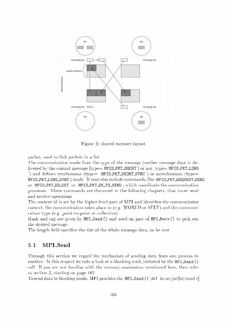
packet memory

incoming list

incoming listincoming list

incoming list NULL

P1 P2

P4P3

shar

ed m

emor

y

Figure 2: shared memory layoutpacket, used to link packets in a list.The communication mode �xes the type of the message (wether message data is de-livered by the control message [type= MPID PKT SHORT ] or not [type= MPID PKT LONG]) and de�nes synchronous (type= MPID PKT SHORT SYNC ) or asynchronous (type=MPID PKT LONG SYNC ) mode. It may also include commands, like MPID PKT REQUEST SENDor MPID PKT DO GET or MPID PKT OK TO SEND , which coordinate the communicationprocesses. These commands are discussed in the following chapters, that cover sendand receive operations.The context id is set by the higher-level part of MPI and identi�es the communicatorcontext, the communication takes place in (e.g. WORLD or SELF) and the communi-cation type (e.g. point-to-point or collective).Rank and tag are given by MPI Send() and used on part of MPI Recv() to pick outthe desired message.The length �eld speci�es the size of the whole message data, to be sent.5.1 MPI SendThrough this section we regard the mechanism of sending data from one process toanother. In this respect we take a look at a blocking send, initiated by the MPI Send()call. If you are not familiar with the memory oranisation mentioned here, then referto section 3, starting on page 102.To send data in blocking mode, MPI provides the MPI Send() [def. in src/pt2pt/send.c]104

call. When called, MPI Send() �rst creates an shandle. The information about the des-tination rank, the tag, datatype of the bu�er, communicator (see glossary) , pointerto the bu�er, length of bu�er, the rank of the sender and several other information notmentioned here are stored in this shandle. After that, MPI Send() creates and setupsa dhandle by setting the pointer of the bu�er and the number of bytes to be copied24.Therefore we have two handles: shandle and dhandle. The dhandle is the device's ver-sion of the shandle and is placed within the structure of the shandle. The lower-levelpart mainly uses this dhandle and also modi�es it! It is of type MPID SHANDLEand de�ned in mpid/ch shmem/dmshmem.h. shandle is mainly used by the higher-level part and it is de�ned in include/mpir.h.After initializing shandle and dhandle, MPID SHMEM post send() [def. inmpid/ch shmem/shmemsend.cand then MPID SHMEM complete send() [def. in mpid/ch shmem/shmemsend.c] arecalled(provided that the agMPID LIMITED BUFFERS isn't set when compilingMPI. If it is set, thenMPID SHMEM Blocking send() [def. inmpid/ch shmem/shmemsend.c] is called, whichmarks the send process as nonblocking and then also calls MPID SHMEM post send()and MPID SHMEM complete send()). Both functions get the dhandle of the requestedsend (MPID SHMEM post send() also gets the shandle) and thus have all information,which are necessary to handle the send.The task of MPID SHMEM post send() is to start (not to �nish) the send. Dependingon the size of the message data, MPID SHMEM post send() either begins a short send25(via MPID SHMEM post send short() [def. in mpid/ch shmem/shmemsend.c] ) or along send (via MPID SHMEM post send long get() [def. inmpid/ch shmem/shmemsend.c]). At �rst both functions allocate a packet in the shared memory region using MPID SHMEM GetSendPkt()[def. in mpid/ch shmem/shmempriv.c] (the short version creates an packet of typeMPID PKT SHORT T [def. in mpid/ch shmem/packets.h], the long version oftype MPID PKT GET T[def. inmpid/ch shmem/packets.h], which carries additional information).MPID SHMEM GetSendPkt() simply tries to get a free packet from the avail list26. If itfails to get one, MPID SHMEM GetSendPkt() waits until a process gives a packet backto the related sender.After allocation, mode, context id, local rang, tag, pointer to and the length of the mes-sage data are stored in the packet. Additionally MPID SHMEM post send long get()sets up a send id , receive id , the length of the delivered partial message dataand the pointer to that part of the message data, not sent by now. Their meaningswill be discussed next.In case of a short send, the message data is copied into a bu�er placed in the packet.Then, MPID SHMEM post send short() calls MPID SHMEM SendControl() [def. inmpid/ch shmem/shmempriv.c] (MPID SENDCONTROL). The MPID SHMEM SendControl()function just inserts the packet into the incoming list of the receiver. After that, thesend is marked as completed (in the shandle and therefore visible from the higher-level24the number of bytes is calculated with regard to the given datatype25that means that the message data may �t in the control message. See also section 3, starting onpage 10326see section "Usage of Shared Memory" 105

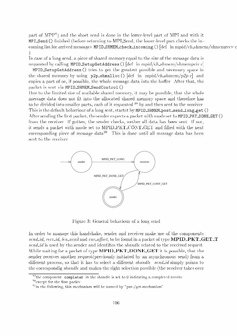
part of MPI27) and the short send is done in the lower-level part of MPI and with itMPI Send() �nished (before returning to MPI Send, the lower-level part checks the in-coming list for arrived messages MPID SHMEM check incoming() [def. inmpid/ch shmem/shmemrecv.c]).In case of a long send, a piece of shared memory equal to the size of the message data isrequested by calling MPID SetupGetAddress() [def. inmpid/ch shmem/shmempriv.c]. MPID SetupGetAddress() tries to get the greatest possible and necessary space inthe shared memory by using p2p shmalloc() [def. in mpid/ch shmem/p2p.c] andcopies a part of or, if possible, the whole message data into the bu�er. After that, thepacket is sent via MPID SHMEM SendControl().Due to the limited size of available shared memory, it may be possible, that the wholemessage data does not �t into the allocated shared memory space and therefore hasto be divided into smaller parts, each of it requested 28 by and then sent to the receiver.This is the default behaviour of a long sent, startet by MPID SHMEM post send long get().After sending the �rst packet, the sender expects a packet with mode set to MPID PKT DONE GET()from the receiver. If gotten, the sender checks, wether all data has been sent. If not,it sends a packet with mode set to MPID PKT CONT GET and �lled with the nextcorresponding piece of message data29. This is done until all message data has beensent to the receiver.sender

receiverMPID_PKT_LONG

MPID_PKT_DONE_GET

MPID_PKT_CONT_GET

sender

Figure 3: General behaviour of a long sendIn order to manage this handshake, sender and receiver make use of the componentssend id, recv id, len avail and cur o�set, to be found in a packet of typeMPID PKT GET T.send id is used by the sender and identi�es the shandle related to the received request.While waiting for a packet of typeMPID PKT DONE GET it is possible, that thesender receives another request(previously initiated by an asynchronous send) from adi�erent process, so that it has to select a di�erent shandle. send id simply points tothe correspondig shandle and makes the right selection possible (the receiver takes over27the component completer in the shandle is set to 0 indicating a completed receive28except for the �rst packte29in the following, this mechanism will be named by "put-/get-mechanism"106

the send id from the received packet and stores it in theMPID PKT DONE GET-packet).recv id gives the matching receive handle (rhandle) on part of the receiver. Its initialvalue 0 tells the receiver, that it is the �rst packet of a new send.The size of the partial message data, delivered by a packet, is stored in len avail andcur o�set points to the data, that has to be sent through the next send.As already mentioned, MPID SHMEM post send short() sets up these components andcallsMPID SHMEM SendControl() to insert this packet in the incoming list of the receiver.After that, it assigns MPID CMPL SEND GET to a ag in the shandle (the com-ponent completer), which indicates, that there is a send, not yet �nished. Then, return-ing to MPID SHMEM post send(),MPID SHMEM check incoming() is called to receive the expectedMPID PKT DONE GETpacket as response by the receiver. If arrived, MPID SHMEM check incoming() usesMPID SHMEM Done get() [def. in mpid/ch shmem/shmemget.c] , to either deliver thenext part of the message data or to mark the sending process as completed throughsetting component completer of the shandle equal to 0. It should be mentioned here,that MPID SHMEM Done get() allocates a new packet via MPID SHMEM GetSendPkt()[def. in mpid/ch shmem/shmempriv.c] when sending the next piece of message datainstead of reusing the received packet.5.2 MPI RecvIn this section we do not want to describe a blocking receive operation in great detail,because its function can be deduced from the behaviour of a blocking send (throughMPI Send(). See previous section). Especially we take a look at the treatment ofmultiple packets, not necessary relating to each other30, by the MPI Recv() call.A blocking receive can be done by the MPI Recv() [def. in src/pt2pt/recv.c] call.Like MPI Send(), it creates a handle, called rhandle, in which it stores the tag, con-text identi�cator, communicator, the datatype of the message data and a pointer tothe bu�er, to be �lled with the message data and the length of the message data.This information is used to pick out the expected message from "pool" of arrived mes-sages. In analogy to MPI Send(), it also creates a handle for the lower-level part -the dev rhandle - and setups its �elds. Then, MPID SHMEM blocking recv() [def. inmpid/ch shmem/shmemrecv.c] (MPID Blocking recv) is called, with the corre-sponding rhandle passed to it.Before continuing, let us imagine a situation, in which multiple messages of severalprocesses have been arrived. How are these messages handled, when MPI Recv() isstarted? In this respect remember, that the shared memory region is of limited spaceand that each sender expects the receiver to give back the packet after its evaluation31.The given question will be regarded in the following.When called, MPID SHMEM blocking recv() �rst uses MPIR search unexpected queue()30that means, caused by di�erent processes for example31see section "MPI Send" for more information about allocating and freeing space for packets107

[def. in src/util/mpirutil.c] (DMPI search unexpected queue) to search the socalled unexpected queue in order to �nd a rhandle containing a message, that corre-sponds to the one, speci�ed by the MPI Recv call. If found, the rhandle will be removedfrom the unexpected queue and after that,MPID SHMEM blocking recv() calls MPID SHMEM Process unexpected get() [def. inmpid/ch shmem/shmemget.c] to complete the receiving procedure and to copy themessage data into the receiver's bu�er and to store information about the message(source, tag, length) in the rhandle, speci�ed through the MPI Recv() call (the rhan-dle stored in the unexpected queue, does not necessary have to be one, that is givenby MPI Recv(), because when a process receives a packet, for which it does not have arhandle32, it creates a rhandle, �lls it with the information about the received packetand inserts this rhandle into the unexpected queue ).Remember that, due to the length of the message data, it may be necessary to splitthe message data into several pieces and send each piece explicitly 33. Therefore,MPID SHMEM Process unexpected get() uses the function MPID SHMEM complete recv()[def. in mpid/ch shmem/shmemrecv.c] , which handles subsequent put-/get-transfersthrough MPID SHMEM check incoming() in order to get the missing message data fromthe sender. The put-/get-mechanism is descriped in section "MPI Send".If the message was not in the unexpected queue , MPID SHMEM blocking recv()reads the next available packet through MPID SHMEM ReadControl() [def. inmpid/ch shmem/shmempriv.c](MPID PKT POST AND WAIT). First, MPID SHMEM ReadControl() checks the localqueue34 for available packets and if none existing, it checks the incoming queue. If thereis also no packet, MPID SHMEM ReadControl() waits for an incoming packet.After obtaining a packet, MPID SHMEM blocking recv() looks up, wether this packet isthe one, the user expects to get. If so, the message is read in its whole by MPID SHMEM Copy body()followed by MPID SHMEM complete recv().In case of an unexpected packet, the packet is inserted in the unexpected queue viaDMPI msg arrived() [def. in src/dmpi/dmpi.c] . For that reason, when MPID SHMEM blocking recv()is called, the unexpected queue is searched at �rst (refer to the begining of this sec-tion).It is also possible, that MPID SHMEM ReadControl() returns a packet of typeMPID PKT CONT GET(which results from another receive) or of typeMPID PKT DONE GET (by whichanother process signals a completed receive). In case ofMPID PKT CONT GET35the message data of the corresponding packet will be copied into the bu�er, that isgiven by the related rhandle. Otherwise (MPID PKT DONE GET36), the nextpiece of message data 37will be sent to the receiver.32because there hasn't been a matching receive since33refer to section "MPI Send" starting on page 10434the local queue is process-local. As soon as possible, packets are removed from the incomingqueue and placed in the local queue. The local queue is not visible to other processes, so that atomicoperations are not necessary to modify it35given by a sender, who sent the next piece of message data36given by a receiver to acknowledge the receive of a piece of message data37if existing 108

6 Nonblocking Send And ReceiveIn MPI, an nonblocking send is initiated using MPI Isend()38 and �nished by MPI Wait()on part of the sender. The receiver calls MPI Irecv() and then MPI Wait() to receivea message in nonblocking mode.MPI Isend() [def. in src/pt2pt/isend.c] creates a shandle and a dhandle and then ini-tializes the shandle39. This is done by calling MPI Send init() [def. in src/pt2pt/create send.c]. After that, by calling MPI Start() [def. in src/pt2pt/start.c] , MPI Isend() setsup the components of the dhandle and starts a put-/get-mechanism through using thefunction MPID SHMEM post send() [def. in mpid/ch shmem/shmemsend.c] 40. Then,MPI Isend() returns back, returning shandle to the caller.To �nish a started nonblocking send, the user has to call MPI Wait(), that, with respectto MPI Isend(), has to �nish a put-/get-process. Therefore MPI Waitall() [def. insrc/pt2pt/waitall.c] (simply called by MPI Wait) refers to MPID SHMEM complete send()[def. inmpid/ch shmem/shmemsend.c] , that on its part uses MPID SHMEM check incoming()[def. in mpid/ch shmem/shmemrecv.c] to respond to each incoming packet of typeMPID PKT DONE GET and as a result, completes all open sends by sending allmissing pieces of message data.On the other side, the receiver uses MPI Irecv() to start a nonblocking receive. LikeMPI Isend(), it creates a rhandle and a dhandle, initializes the rhandle and thencalls MPI Start(). This time MPI Start() calls MPID SHMEM post recv() [def. inmpid/ch shmem/shmemrecv.c](MPID Post recv) 41. MPID SHMEM post recv() starts with searching the unexpectedqueue for the desired message. If a matching packet was found, MPID SHMEM Process unexpected get()is called, which completes the whole receive.If it is not in the unexpected queue , MPID SHMEM post recv() simply adds therhandle to the so called posted receive queue and the receiving process is done.In order to �nish a nonblocking receive, the user also utilizes MPI Waitall() (viaMPI Wait()), which ends the receiving process by calling MPID SHMEM complete recv()[def. inmpid/ch shmem/shmemrecv.c] (MPID Complete recv).MPID SHMEM complete recv() frequently refers to MPID SHMEM check incoming() un-til the given receive is completed. Regarding MPID SHMEM check incoming(), theremight be a problem: To which rhandle does it has to assign the �rst packet of a newreceive ? Remember, that in contrast to a MPI Recv(), we do not explicitly waitfor a speci�c packet and so do not have any rhandle ready. The rhandles of non-blocking receives are to be found in the posted receive queue . So if the �rstpacket of a new receive arrives (e.g. a packet of type MPID PKT DO GET),MPID SHMEM complete recv() searches the posted receive queue to get the corre-38also possible: MPI Issend() (synchronous, nonblocking send), MPI Ibsend() (bu�ered, nonblock-ing), MPI Irsend() (ready, nonblocking)39for detailed information, please refer to section "MPI Send", starting on page 10440this function and the put-/get-mechanism are mentioned in section "MPI Send"41the di�erent behaviour of MPI Start() depends on the type of the given handle (send-/receive-handle) 109

sponding rhandle and after that, it calls MPID SHMEM Do get() [def. inmpid/ch shmem/shmemget.c]to copy the message data, stored in the packet, into the receivers bu�er, determinedby the rhandle. Next, it sets recv id of the packet equal to the pointer to the rhan-dle and sends it back with mode set to MPID PKT DONE GET. If the senderexpects to send the next piece of message data, then it delivers a packet of typeMPID PKT CONT GET, which holds the recv id of the previous gottenMPID PKT DONE GETpacket. Through this mechanism, when getting another piece of data (where thepacket is of type MPID PKT CONT GET), the receiver just has to read therecv id to get the corresponding rhandle and as a result it has to search the postedreceive queue only when receiving the �rst packet of a new receive (e.g. of typeMPID PKT DO GET).7 Broadcast and Reduce OperationsAlthough broadcast and reduce operations are not supported by the general sharedmemory device and therefore realized by the higher-level part of MPI, we regard theseoperations, because there is a special implementation for convex machines42, makinguse of shared memory.In MPI, reduce operations may start by the MPI Reduce() [def. in src/coll/reduce.c]function, which calls the corresponding reduce function through an array of function-pointers, pointed by communicator->collops. Assuming, that the reduce operationtakes place within one communicator. In this case, communicator->collops points tothe array intra collops [def. in src/coll/intra fns.c] (otherwise to inter collops [def. insrc/coll/inter fns.c]), so that intra Reduce() [def. in src/coll/intra fns.c] is calledin this context.This function uses a tree-structured communication, in which each node uses blockingsend and receive operations(via MPI Send() and MPI Receive()).Similar to MPI Reduce(), MPI Broadcast() refers to intra Bcast() [def. in src/coll/intra fns.c]via communicator->collops and also uses a tree-structured communication and block-ing send and receive operations.MPI Allreduce() [def. in src/coll/allreduce.c] does its work by calling MPI Reduce()(with root=proc 0) and MPI Bcast() ( with root=proc ) following.If given explicitly43, MPI Reduce() and/or MPI Bcast() may refer to functions of thelower-level part. This is done in case of using the shared memory device on a convexmachine44, whereMPID SHMEM Reduce() [def. inmpid/ch shmem/shmemcoll.c] and/or MPID SHMEM Bcast()[def. inmpid/ch shmem/shmemcoll.c] are executed.The algorithm, MPID SHMEM Reduce() uses, depends on the size of the given send-42based on the shared memory device43that means, if, during compile-time, the macrosMPID FN Bcast andMPID FN Reduce areset to the corresponding functions in the lower-level part44so that the macro MPI cspp is set 110

bu�er and therefore on count 45. If count is less than the number of the participatingprocesses, then MPID SHMEM Reduce() calls MPID SHMEM Small reduce(). Otherwisethe data will be parted in regions of equal size and each process operates over one byreading the related regions from all processes and storing the results into the root's46bu�er. So each process has to copy its sendbu�er into the shared memory and makeit visible to the other processes. To realize the visibility of the copied sendbu�er, eachprocess saves the related pointer into its barrier- ag, which can be read by all processes.MPID SHMEM Small reduce() [def. inmpid/ch shmem/shmemcoll.c] uses a tree-structuredcommunication. It also refers to barriers in order to realize the communication andcoordination of the calculating procedure. The barrier ag is used to indicate, wetherthe concerning process has its result ready or not and the pointer to the barrier ag(which is also visible by all processes) is set to the pointer of the region, holding theresult. Therefore each node(=process) waits for its subnodes to get ready, by regardingtheir barrier ags47 and then calculates over the given operands and sets its barrier ag itself equal to null48. When this is done up to the root process, the root process49starts to cancel the barrier and �nishes MPI Reduce() with the desired result.In the devices version of MPI Reduceall(), each process calculates over a partial re-gion and put the result in its bu�er (this algorithm is similar to the one, mentionedabove). After that, all processes gather the partial results from each other.

45see MPI Reduce-call46determined by MPI Reduce-call()47set to null, if ready48which causes the process to block49and with it, all other processes 111

8 ConclusionThrough the last sections, we pointed out several features of the shared memory device,including important data structures, like MPID SHMEM globmem, basic functionali-ties like the put-/get-mechanism, the interaction between the lower- and the higher-level part, e.g. explained in section "Nonblocking Send and Receive" and the usageof the shared memory, especially shown in sections "Usage of Shared Memory" and"Broadcast and Reduce Operations". The corresponding descriptions should give anorientation through the implementation and by mentioning necessary names, locations,etc., it may also serve as a reference, while working on the implementation.At the end, the author wants to note several characteristics, which are describedby the sections and which may be of interest for future developement, concerninga mulithreaded MPI:� Due to its process-oriented design, each communication results in two memorytransfers: sender to shared memory and receiver from shared memory. For amultithreadedMPI, where all communicators take place in the same adress space,only one copy operation is necessary. This can be realized by just "sending" thepointer to the send-bu�er.� The underlying shared memory is allocated only at the initial process from thesystem and then organized by the device itself. This organization can be left outin a multithreaded enviroment.� The size of the shared memory is limited (see section "Usage of Shared Memory",starting on page 102) and as a result, large message data is split into severalpackets and delivered by a done-/get- mechanism. The splitting and done-/get-mechanism can be simpli�ed, by sending the pointer to the sendbu�er50 and onpart of the receiver, copying the bu�er by only one operation in its whole.� The whole treatment of the packets may be simpli�ed, regarding their allocationand deallocation� The collective operations, like MPI Broadcast() and MPI Reduce(), which cur-rently are only optimized for convex machines, should also be implemented in amultithreaded version.� A multithreaded MPI may also include put- and get- operations, which are notpart of the current MPI speci�cation.50as mentioned before 112

References[1] NFS ARPA and other. Message Passing Interface, 1994. available via ftp frominfo.mcs.anl.gov/pub/mpi.[2] William Gropp. MPICH ADI Implementation Reference Manual, 1995. availablevia ftp from ftp.anl.gov/pub/mpi �le adiman.ps.[3] Ewing Lusk?? Creating a new MPICH device, 1995. available via ftp fromftp.anl.gov/pub/mpi/workingnote �le newadi.ps.[4] Peter S. Pacheco. A User's Guide to MPI, 1995.[5] Anthony Skjellum William Gropp, Ewing Lusk. Portable Parallel Program-ming with the Message-Passing Interface, 1994. available via ftp fromhttp://www.mcs.anl.gov/mpi/usingmpi/index.html.

113

9 GlossaryADI The Abstract Device Interface. It de�nes the core message passing routinesand other system-related features and therefore lets the higher-level part of MPIabstract from features, speci�c to the system.MPI COMM WORLD In MPI, so called communicators de�ne the scope in whicha communication operator may have its e�ect. This scope is determined by agroup of processes ( process group ) and by a context (which contains localinformation of a communicator). Together, group and context build a communi-cator. MPI COMM WORLD is such a communicator, prede�ned by the initial process(see p. 101). It stores references to all processes start up at initial sequence. (fordetailed description see [1, p. 133�])MPI COMM SELF Prede�ned communicator (like MPI COMM WORLD), onlyconsisting of the process itself.control message In MPI, each message data is bound to a control message whichdescribes the underlying protocol, used when sending the message data, thelength of the data etc. See also p. 103.packet A packet is used by the low-level part of MPI and enables send/receive requestsby exchanging packets through the shared memory region. It contains the sendingmode51, a context identi�er, the local rank of the sending process, the pointer tothe bu�er, holding the message data, the length of the message data and otherinformation, depending on the sending/receiving mode. For detailed descriptionsee �le mpid/ch shmem/packets.h, esp. look at type MPID PKT T , where youcan see all possible types of packets.51for example "short" or "long" 114

Principles of Parallel Computers and some Impactson their Programming ModelsThomas Radke Wolfgang Rehmtomsoft@informatik.tu-chemnitz.de rehm@informatik.tu-chemnitz.dehttp://noah.informatik.tu-chemnitz.de/members/radke/radke.html http://noah.informatik.tu-chemnitz.de/members/rehm/rehm.htmlAbstractIn this paper we brie y outline some principles of parallel architectures anddiscuss several impacts on their programming models. At �rst, parallel comput-ers are generally classi�ed. A description of the most important classes { Mul-tiprocessors and Massively Parallel Systems { follows, with some details aboutchosen machines. The corresponding programming models for shared memoryand distributed memory architectures are introduced. The special relationshipbetween machine architecture and e�cient parallel programming is emphasizedhere. The paper concludes with some hints for the software developer where touse which parallel programming model.1 IntroductionThe last ten years have seen the employment of parallel computers for the solutionof complex scienti�c, mathematical, and technical problems developing into key tech-nology. The paradigm shift towards parallelism has led to changes on all levels, frommachine hardware to application programs. A broad spectrum of parallel architectureshas been developed.In general, a parallel algorithm can only be e�ciently implemented if it is designedfor the speci�c needs of the architecture. Thus the knowledge of primary computerdesign principles is of course relevant for software developers as well as numericalanalysts in the �eld of computational physics. This fact is often underestimated bysoftware developers.For this reason in the following we present a brief introduction into basic architec-tures of parallel computers.2 Overview on Architecture PrinciplesBefore the development of \vector computers" in the 1970s, so-called \mainframes"were also used for scienti�c computing although they have typically been the workhorsesof data processing departments.The �rst supercomputer architectures involved the use of one { or, at most, a few {of the fastest processors that could be obtained by increasing the packing density, min-115

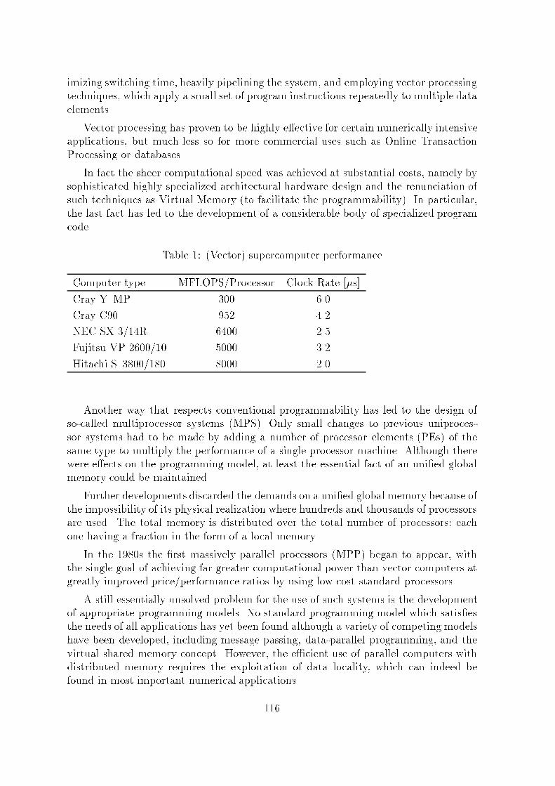
imizing switching time, heavily pipelining the system, and employing vector processingtechniques, which apply a small set of program instructions repeatedly to multiple dataelements.Vector processing has proven to be highly e�ective for certain numerically intensiveapplications, but much less so for more commercial uses such as Online TransactionProcessing or databases.In fact the sheer computational speed was achieved at substantial costs, namely bysophisticated highly specialized architectural hardware design and the renunciation ofsuch techniques as Virtual Memory (to facilitate the programmability). In particular,the last fact has led to the development of a considerable body of specialized programcode. Table 1: (Vector) supercomputer performanceComputer type MFLOPS/Processor Clock Rate [�s]Cray Y{MP 300 6.0Cray C90 952 4.2NEC SX 3/14R 6400 2.5Fujitsu VP 2600/10 5000 3.2Hitachi S{3800/180 8000 2.0Another way that respects conventional programmability has led to the design ofso-called multiprocessor systems (MPS). Only small changes to previous uniproces-sor systems had to be made by adding a number of processor elements (PEs) of thesame type to multiply the performance of a single processor machine. Although therewere e�ects on the programming model, at least the essential fact of an uni�ed globalmemory could be maintained.Further developments discarded the demands on a uni�ed global memory because ofthe impossibility of its physical realization where hundreds and thousands of processorsare used. The total memory is distributed over the total number of processors; eachone having a fraction in the form of a local memory.In the 1980s the �rst massively parallel processors (MPP) began to appear, withthe single goal of achieving far greater computational power than vector computers atgreatly improved price/performance ratios by using low cost standard processors.A still essentially unsolved problem for the use of such systems is the developmentof appropriate programming models. No standard programming model which satis�esthe needs of all applications has yet been found although a variety of competing modelshave been developed, including message passing, data-parallel programming, and thevirtual shared memory concept. However, the e�cient use of parallel computers withdistributed memory requires the exploitation of data locality, which can indeed befound in most important numerical applications.116

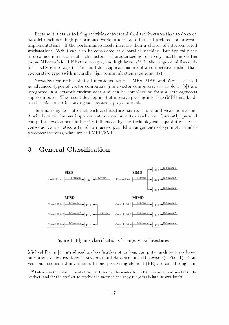
Because it is easier to bring activities onto established architectures than to do so onparallel machines, high-performance workstations are often still prefered for programimplementations. If the performance needs increase then a cluster of interconnectedworkstations (WSC) can also be considered as a parallel machine. But typically theinterconnection network of such clusters is characterized by relatively small bandwidths(some MBytes/s for 1 KByte messages) and high latency52 (in the range of millisecondsfor 1 KByte messages). Thus suitable applications are of a competitive rather thancooperative type (with naturally high communication requirements).Nowadays we realize that all mentioned types { MPS, MPP, and WSC { as wellas advanced types of vector computers (multivector computers, see Table 1, [5]) areintegrated in a network environment and can be combined to form a heterogeneoussupercomputer. The recent development of message passing interface (MPI) is a land-mark achievement in making such systems programmable.Summarizing we note that each architecture has its strong and weak points andit will take continuous improvement to overcome its drawbacks. Currently, parallelcomputer development is heavily in uenced by the technological capabilities. As aconsequence we notice a trend to massive parallel arrangements of symmetric multi-processor systems, what we call MPP/SMP.3 General Classi�cationControl Unit

Control Unit 1

Control Unit 2

Control Unit n Control Unit n

Control Unit 2

Control Unit 1

Control UnitD-Stream

D-Stream n

D-Stream 2

D-Stream 1

D-Stream n

D-Stream 2

D-Stream 1PE 1

PE 2

PE n

PE 1

PE 2

PE nI-Stream n

I-Stream 2

I-Stream 1

I-Stream

SIMD

MIMD

SISD

MISD

I-StreamPE

PE 1

PE 2

PE nI-Stream n

I-Stream 2

I-Stream 1

D-StreamFigure 1: Flynn's classi�cation of computer architecturesMichael Flynn [6] introduced a classi�cation of various computer architectures basedon notions of instructions (I{streams) and data streams (D{streams) (Fig. 1). Con-ventional sequential machines with one processing element (PE) are called Single In-52Latency is the total amount of time it takes for the sender to pack the message and send it to thereceiver, and for the receiver to receive the message and copy (unpack) it into its own bu�er.117

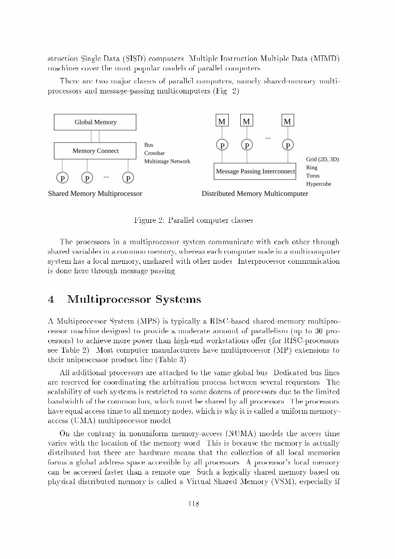
struction Single Data (SISD) computers. Multiple Instruction Multiple Data (MIMD)machines cover the most popular models of parallel computers.There are two major classes of parallel computers, namely shared-memory multi-processors and message-passing multicomputers (Fig. 2).Memory Connect

P PP

Global Memory

...

Bus

Crossbar

Multistage Network

M

P

M

PP

Grid (2D, 3D)

Ring

Torus

Hypercube

Message Passing Interconnect

M

...

Distributed Memory MulticomputerShared Memory MultiprocessorFigure 2: Parallel computer classesThe processors in a multiprocessor system communicate with each other throughshared variables in a commonmemory, whereas each computer node in a multicomputersystem has a local memory, unshared with other nodes. Interprocessor communicationis done here through message passing.4 Multiprocessor SystemsA Multiprocessor System (MPS) is typically a RISC-based shared-memory multipro-cessor machine designed to provide a moderate amount of parallelism (up to 30 pro-cessors) to achieve more power than high-end workstations o�er (for RISC-processorssee Table 2). Most computer manufacturers have multiprocessor (MP) extensions totheir uniprocessor product line (Table 3).All additional processors are attached to the same global bus. Dedicated bus linesare reserved for coordinating the arbitration process between several requestors. Thescalability of such systems is restricted to some dozens of processors due to the limitedbandwidth of the common bus, which must be shared by all processors. The processorshave equal access time to all memory nodes, which is why it is called a uniformmemory-access (UMA) multiprocessor model.On the contrary in nonuniform memory-access (NUMA) models the access timevaries with the location of the memory word. This is because the memory is actuallydistributed but there are hardware means that the collection of all local memoriesforms a global address space accessible by all processors. A processor's local memorycan be accessed faster than a remote one. Such a logically shared memory based onphysical distributed memory is called a Virtual Shared Memory (VSM), especially if118

Table 2: Performance of some RISC CPUsCPU Type Clock Rate Perf. CPU Type Clock Rate Perf.[MHz] [MIPS] [MHz] [MIPS]Alpha 21164 300 1200 MPC601 80 240MPC604 100 400 MPC620 133 532SuperSparc 60 180 UltraSparc 167 668PA7200 140 280 R4400SC 150 150R10000 200 800 MC68060 50 100Pentium 100 100 200 Pentium Pro 133 399Table 3: Multiprocessor systemsCompany Model Scalability I/O Bus[processors] Type BandwidthSequent Symmetry 5000 1: : :30 symm. 240 MByte/sSilicon Graphics PowerChallenge 1: : :30 symm. 1.2 GByte/sSun SPARCstat. 20 HS14 1: : :4 symm. {Compaq ProLiant 4000 1: : :4 symm. 267 MByte/sthere is essential hardware support to realize this (Fig. 3). One special version of aVSM architecture is a cache-only memory architecture (COMA) such as in the KSR-1machine (Fig. 4 [2]). Caches copy data from other caches if necessary. There is acontinuous process of data migration. A cache attracts the needed data, and in theideal case the user is completely freed from prede�ning the data layout.Drawbacks of such wonderful architectures lie in the synchronization costs for main-taining the cache coherency as well as the global synchronization (via semaphores). Forfurther modi�cations of COMA models see [8].Another distinction can be made between asymmetric and symmetric multiproces-sor systems (Fig. 5). When all processors have equal access to all peripheral devices thesystem is called a symmetric multiprocessor (SMP). All processors are equally capableof running the executive programs, such as the operating system kernel and I/O ser-vice routines. In asymmetric systems only a master processor can execute the OS andhandle I/O. Thus I/O becomes a bottleneck. Such systems we �nd today often in formof two-processor stations whereas symmetric solutions signify 4-processor board-basedworkstations or servers (Table 3).To overcome the drawbacks of limited speed of a uni�ed common global bus, connec-tion schemes with crossbar technology have recently been developed [3]. The advantage119

... ...

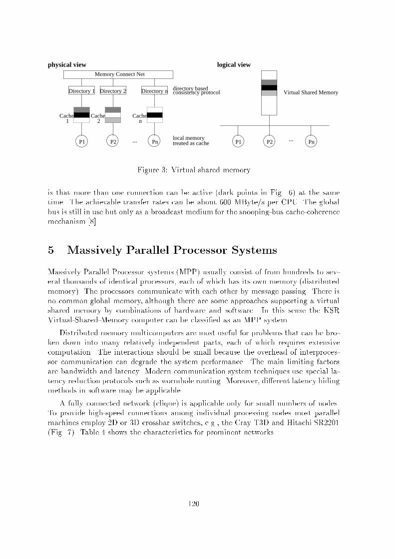
Memory Connect Net

directory basedconsistency protocol

PnP2local memorytreated as cache P1 P2 Pn

Virtual Shared Memory

P1

Directory 1 Directory 2 Directory n

Cache Cache Cache1 2 n

physical view logical view

Figure 3: Virtual shared memoryis that more than one connection can be active (dark points in Fig. 6) at the sametime. The achievable transfer rates can be about 600 MByte/s per CPU. The globalbus is still in use but only as a broadcast medium for the snooping-bus cache-coherencemechanism [8].5 Massively Parallel Processor SystemsMassively Parallel Processor systems (MPP) usually consist of from hundreds to sev-eral thousands of identical processors, each of which has its own memory (distributedmemory). The processors communicate with each other by message passing. There isno common global memory, although there are some approaches supporting a virtualshared memory by combinations of hardware and software. In this sense the KSRVirtual-Shared-Memory computer can be classi�ed as an MPP system.Distributed memory multicomputers are most useful for problems that can be bro-ken down into many relatively independent parts, each of which requires extensivecomputation. The interactions should be small because the overhead of interproces-sor communication can degrade the system performance. The main limiting factorsare bandwidth and latency. Modern communication system techniques use special la-tency reduction protocols such as wormhole routing. Moreover, di�erent latency hidingmethods in software may be applicable.A fully connected network (clique) is applicable only for small numbers of nodes.To provide high-speed connections among individual processing nodes most parallelmachines employ 2D or 3D crossbar switches, e.g., the Cray T3D and Hitachi SR2201(Fig. 7). Table 4 shows the characteristics for prominent networks.120

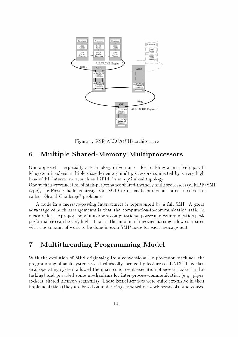
Processor

Directory

LocalCache

LocalCache

Processor

Directory

LocalCache

LocalCache

Processor

Directory

LocalCache

LocalCache

ARD

Directory

ALLCACHEGroup : 0

ALLCACHERouter

Directory

ALLCACHE Engine : 0

ARD

Directory

ALLCACHEGroup : 1

ALLCACHERouter

Directory

ALLCACHE Engine : 1

ARD

Directory

ALLCACHEGroup : 0

Ring 0

Ring 1

Processor

Directory

LocalCache

LocalCache

Figure 4: KSR ALLCACHE architecture6 Multiple Shared-Memory MultiprocessorsOne approach { especially a technology-driven one { for building a massively paral-lel system involves multiple shared-memory multiprocessors connected by a very highbandwidth interconnect, such as HiPPI, in an optimized topology.One such interconnection of high-performance shared-memorymultiprocessors (of MPP/SMPtype), the PowerChallenge array from SGI Corp., has been demonstrated to solve so-called \Grand Challenge" problems.A node in a message-passing interconnect is represented by a full SMP. A greatadvantage of such arrangements is that the computation-to-communication ratio (ameasure for the proportion of maximumcomputational power and communication peakperformance) can be very high. That is, the amount of message passing is low comparedwith the amount of work to be done in each SMP node for each message sent.7 Multithreading Programming ModelWith the evolution of MPS originating from conventional uniprocessor machines, theprogramming of such systems was historically formed by features of UNIX. This clas-sical operating system allowed the quasi-concurrent execution of several tasks (multi-tasking) and provided some mechanisms for inter-process-communication (e.g. pipes,sockets, shared memory segments). These kernel services were quite expensive in theirimplementation (they are based on underlying standard network protocols) and caused121

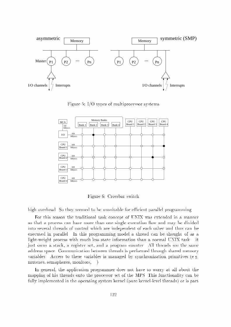
Memory

P1 PnP2

InterruptsI/O channels

Master

InterruptsI/O channels

Memory

P1 PnP2

symmetric (SMP)

...

asymmetric

...Figure 5: I/O types of multiprocessor systemsBoard 1

CPUBoard 1

CPUBank 1 Bank 2 Bank 3 Bank 4

Memory BanksCPU CPU CPU

Board 2 Board 3 Board 4

CPU

CPU

CPU

Board 4

Board 3

I/O

MCA160

MByte/s

MByte/s

MByte/s

MByte/s

MByte/s

MByte/s

600

600

600

600

600

Board 2 Figure 6: Crossbar switchhigh overhead. So they seemed to be unsuitable for e�cient parallel programming.For this reason the traditional task concept of UNIX was extended in a mannerso that a process can have more than one single execution ow and may be dividedinto several threads of control which are independent of each other and thus can beexecuted in parallel. In this programming model a thread can be thought of as alight-weight process with much less state information than a normal UNIX task { itjust owns a stack, a register set, and a program counter. All threads see the sameaddress space. Communication between threads is performed through shared memoryvariables. Access to these variables is managed by synchronization primitives (e.g.mutexes, semaphores, monitors, ...).In general, the application programmer does not have to worry at all about themapping of his threads onto the processor set of the MPS. This functionality can befully implemented in the operating system kernel (pure kernel-level threads) or is part122

Y switch

Z switch

X switch

ElementProcessor

� message transmission network for linking PEs� A crossbar switch consists of 3 crossbars, onefor each axis, to create 2D and 3D structures.� At each level, a crossbar switch is capable ofswitching up to 8�8 connections.� Data transfer rate : 300 MByte/s in each di-rection of the bidirectional portsFigure 7: 3-dimensional crossbar network in the Hitachi SR2201 [1]of a thread library with kernel support (mixed user/kernel level threads).The exclusive use of kernel level threads is reasonable if the number of threads doesnot exceed the number of processors in the system. Each thread is �xed bound to itsown processor and can run fully parallel to others. Synchronization can be implementedas busy waiting (the associated processor is not released but spins on a condition tobecome true).If there are more threads than available processors (and this is the most frequentcase) busy waiting between threads is no longer applicable because of possible dead-locks. In this case synchronization can cause a thread switch on a processor. Theswitching of kernel-level threads can only be done in the kernel, i.e., special systemcalls are needed. The resulting overhead (kernel thread context switch plus enter-ing/leaving the kernel) may drastically decrease the e�ciency of a pure kernel-levelthread management. That is why a mixed thread management is more favourable inthis case: the programmer uses user-level threads which are managed by a thread li-brary; these user-level threads are internally mapped onto some kernel-level threadswith their number corresponding to the number of available processors (see Fig. 8).Thread context switches can now completely be done in user mode, and time-expensivesystem calls are unnecessary.It is true that the problem of optimal load balancing in MPS is not as di�cult as inMPP. Because of the global shared memory every thread can principially be scheduledon any processor without explicite migration. But in NUMA architectures, threadlocality must be taken into consideration for achieving e�cient multithreading. Forinstance, if there are still some thread data in a processor's cache this thread shouldbe scheduled with precedence on that processor again. This technique, called memoryconscious scheduling, is especially used in systems with multi-level memory hierarchies[4]. 123

Table 4: Properties of interconnection networksType Degree Connections Diameter Bisectional Symm.WidthClique N � 1 N(N � 1)=2 1 (N=2)2 yesLinear chain 2 N � 1 N � 1 1 noRing 2 N [N=2] 2 yesBinary tree 3 N � 1 2 ((log2N)� 1) 1 no2D grid 4 2N � 2pN 2(pN � 1) 2pN no2D torus 4 2N 2[pN=2] 2pN yesHypercube log2N N log2N log2N N=2 yesThe e�ciency of I/O intensive multithreaded applications strongly depends on theI/O architecture. In asymmetric systems every I/O operation forces a thread switchonto the master processor (which is capable of serving the request, see Fig. 5). Sothe master may become a bottleneck. Only SMP systems guarantee a scalable I/Operformance because each I/O request can be served on the processor where the threadresides. This circumstance is less decisive for multithreaded programs with a high ratioof computation to communication.At present, there exist a number of modern commercial and noncommercial stan-dard operating systems that support multithreading and symmetric multiprocessing:Solaris 2.x from SUN, Mach, Linux-SMP as public domain software, Windows-NT fromMicrosoft). Research is aimed at the development of a unique multithreading program-ming interface (currently proposed as \POSIX 1003.4a Threads Extension Draft").With this, the application programmer should be able to easily port his programs onany MPS architecture.8 Message Passing Programming ModelMessage passing is the natural programming model for distributed memory architec-tures. It is based on Hoare's CSP concept (communicating sequential processes [7])where an application consists of several sequential tasks that communicate with eachother by exchanging data over communication channels. These tasks are distributedamong the nodes of a MPP and thus are executed in parallel. The communicationchannels are mapped onto the communication network. The communication hardwarein modern MPP systems is capable of operating independently of its assigned computenode so that communication and computation can be done concurrently.The e�ciency of the parallel application is essentially determined by the qualityof mapping the process graph with its communication edges onto the underlying dis-124

P P P

user level thread library

useraddressspace

kernel thread management

Thread 0 Thread 1 Thread n

global variables

addresskernel

spacekthread kthread kthread

hardware

Multithreaded Application

Figure 8: Multithreading with user- and kernel-level threadstributed memory architecture (see Fig. 9). In the ideal case each task gets its ownprocessor, and every communication channel corresponds with a direct physical linkbetween both communication nodes.This can be realized in most cases from the view of available processors in mas-sively parallel systems. However, scalability requires a relatively simple communicationnetwork (2D, 3D grid, ring, torus) so at this point compromises are unavoidable. Forinstance, a logical communication channel is routed when it passes one or more gridpoints. This transfer of data takes time especially if there is no hardware support andthe routing must be done by software emulation.On the one hand, communication paths with di�erent delays arise by nonoptimalmapping of communication channels onto the network, on the other hand several logicalchannels are multiplexed on one physical link. From the application programmer'spoint, the usable communication bandwidth is decreased.Since the beginning of the development of MPP, algorithms for various applicationclasses with static problem sizes emerged that �nd the optimal mapping scheme for agiven machine topology and thus allow best exploitation of hardware performance. Theidentical transformation on other topologies is often combined with a loss of e�ciency.That is why porting a parallel application requires at least some basic knowledge fromthe programmer about the target architecture.In recent years research activities were extended to the �eld of adaptive parallelalgorithms development, i.e., of those application classes for which the process graphis adapted to the problem size dynamically. The decision of how to inbed the actualprocess graph into the processor graph cannot be made statically at compile time but125

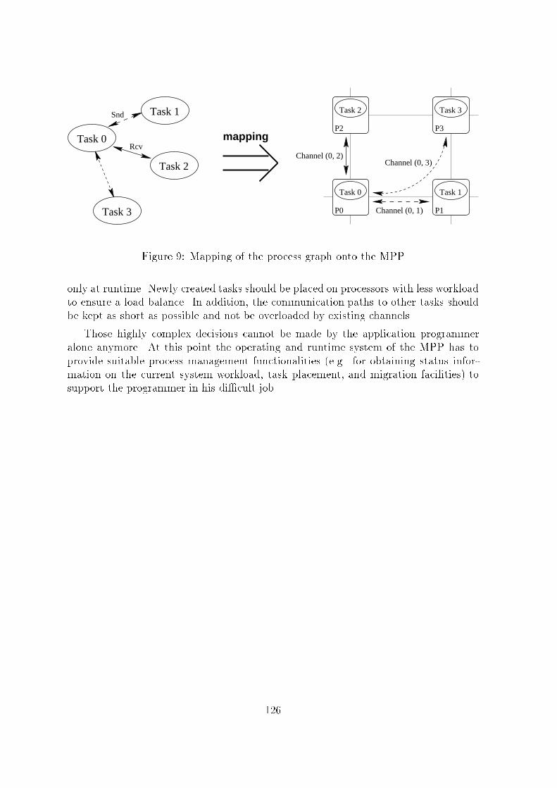
Task 3

Task 0

Task 1

Task 2

Rcv

Snd

mapping

Task 0

Task 3

Task 1

Task 2

P2

P1

P3

P0 Channel (0, 1)

Channel (0, 2)Channel (0, 3)Figure 9: Mapping of the process graph onto the MPPonly at runtime. Newly created tasks should be placed on processors with less workloadto ensure a load balance. In addition, the communication paths to other tasks shouldbe kept as short as possible and not be overloaded by existing channels.Those highly complex decisions cannot be made by the application programmeralone anymore. At this point the operating and runtime system of the MPP has toprovide suitable process management functionalities (e.g. for obtaining status infor-mation on the current system workload, task placement, and migration facilities) tosupport the programmer in his di�cult job.

126

9 SummaryParallel machines can be classi�ed as multiprocessors and massively parallel systems.These classes di�er in the scale of parallelism and the memory architecture. Whilemultiprocessors have equal access to a global shared memory and thus are limited inprocessor number, the latter are scalable to hundreds up to thousands of processorswith each node having its own local memory.The hardware architecture determines the way in which the parallel computer isprogrammed. For multiprocessors the multithreading programming model is prefered.Parallelity in application programs is expressed here as cooperation of several threadsof control which share some global data and synchronize with each other. Messagepassing is used in distributed memory systems. Processes are executed in parallel ondi�erent processor nodes and communicate over channels.The ratio of communication to computation in a parallel program is decisive forits e�ciency. Massively parallel computers provide a high computational power buttypically have a lower communication bandwidth so that I/O intensive applicationsprobably achieve poor performance. For this class of applications Multiprocessors withtheir extremely low communication costs would be better suited. The applicationprogrammer has to keep these facts in mind when implementing his algorithms on atarget architecture.References[1] Hitachi Product Sheet SR2201, Hitachi Corp.[2] KSR Parallel Programming { Manual, (Kendall Square Research Corporation, Mas-sachusetts, 1993)[3] Cross-Bar und Snooping-Bus, iX no. 7, (1995)[4] F. Bellosa, Memory Concious Scheduling and Processor Allocation on NUMA Ar-chitectures, TR{I4{5{95, Computer Science Dep., Univ. Erlangen, (1995)[5] J. Dongarra, Performance of Various Computers using Standard Linear EquationSoftware, Tech. Report January 7, 1995, Computer Science Department, Univ. ofTennessee, Knoxville, (1995)[6] M. Flynn, Some Computer Organizations and their E�ectiveness, IEEE Trans.Computers, no. 21, 948 (1972)[7] C.A.R. Hoare, Communicating Sequential Processes, Prentice Hall, (1989)[8] K. Hwang, Advanced Computer Architecture, Mc Graw-Hill, (1993)127

Redaktion:Fakult�at f�ur InformatikProf. Dr. W. RehmTel.: 0371/531-1420, Fax: 0371/531-1628, e-mail: rehm@informatik.tu-chemnitz.deAssistenz: Dipl. Math. L. Grabowsky, e-mail: grabowsk@informatik.tu-chemnitz.deNachdruck nur mit vollst�andiger Quellenangabe und unter vorheriger Abstimmungmit dem Lehrstuhl \Rechnerarchitektur".