Embed Size (px)
Citation preview

IVE mbH - Infras AG - ifeu - Ingenieurgesellschaft für Consulting, Institut für Energie- Verkehrswesen mbH Analysis and und Umweltforschung Hannover Research Heidelberg GmbH
Ecological Transport Information Tool for Worldwide Transports
Methodology and Data Update
IFEU Heidelberg INFRAS Berne IVE Hannover
Commissioned by
EcoTransIT World Initiative (EWI)
Berne – Hannover – Heidelberg, 4 th December 2014

Page 2 IFEU, INFRAS, IVE
EcoTransIT World: Methodology and Data – Update 4th December 2014
Content
1 Introduction ...................................... ...................................................................... 5
1.1 Background and task ............................... ................................................................... 5
1.2 Accordance with EN 16258 .......................... ............................................................... 6
1.3 ETW business solutions ............................ ................................................................. 8
1.3.1 Soap-xml web service ............................................................................................... 8
1.3.2 Transport list calculation ............................................................................................ 8
1.3.3 ETW on customer website ........................................................................................ 8
1.3.4 Additional features ..................................................................................................... 9
1.3.5 Methodology support included .................................................................................. 9
2 System boundaries and basic definitions ........... ............................................... 10
2.1 Transport service and vehicle operation system .... ............................................... 10
2.2 Environmental impacts ............................. ................................................................ 11
2.3 System boundaries of processes .................... ........................................................ 13
2.4 Transport modes and propulsion systems ............ ................................................. 15
2.5 Spatial differentiation ........................... ..................................................................... 15
3 Basic definitions and calculation rules ........... ................................................... 19
3.1 Main factors of influence on energy and emissions o f freight transport ............ 19
3.2 Logistics parameters .............................. ................................................................... 20
3.2.1 Definition of payload capacity.................................................................................. 21
3.2.2 Definition of capacity utilisation ............................................................................... 25
3.2.3 Capacity Utilisation for specific cargo types and transport modes.......................... 25
3.3 Basic calculation rules ........................... ................................................................... 32
3.3.1 Final energy consumption per net tonne km (TTW) ................................................ 32
3.3.2 Energy related emissions per net tonne km (TTW)................................................. 33
3.3.3 Combustion related emissions per net tonne km (TTW) ......................................... 34
3.3.4 Upstream energy consumption and emissions per net tonne km (WTT) ................ 35
3.3.5 Total energy consumption and emissions of transport (WTW) ............................... 36
3.4 Basic allocation rules ............................ .................................................................... 36
4 Routing of transports ............................. .............................................................. 39
4.1 General ........................................... ............................................................................. 39
4.2 Routing with resistances .......................... ................................................................ 39
4.2.1 Road network resistances ....................................................................................... 39
4.2.2 Railway network resistances ................................................................................... 40
4.3 Sea ship routing .................................. ....................................................................... 41
4.3.1 Routing inland waterway ship.................................................................................. 42
4.4 Aviation routing .................................. ....................................................................... 42

IFEU, INFRAS, IVE Page 3
EcoTransIT World: Methodology and Data – Update 4th December 2014
4.5 Determination of transport points within combined t ransport chains ................. 43
4.5.1 Definition of side tracks for rail transports ............................................................... 44
5 Methodology and environmental data for each transpo rt mode ....................... 45
5.1 Road transport .................................... ....................................................................... 45
5.1.1 Classification of truck types ..................................................................................... 45
5.1.2 Final energy consumption and vehicle emission factors (TTW) ............................. 46
5.1.3 Final energy consumption and vehicle emissions per net tonne km (TTW) ........... 50
5.2 Rail transport .................................... .......................................................................... 53
5.2.1 Train Types.............................................................................................................. 53
5.2.2 Final energy consumption (TTW) ............................................................................ 54
5.2.3 Emission factors for diesel train operation (TTW) ................................................... 60
5.3 Sea transport ..................................... ......................................................................... 61
5.3.1 Overview of the ETW bottom-up approach ............................................................. 61
5.3.2 Development of trade-lane specific emission factors .............................................. 63
5.3.3 Allocation rules for seaborne transport ................................................................... 72
5.3.4 Allocation method and energy consumption for ferries ........................................... 73
5.4 Inland waterway transport ......................... ............................................................... 74
5.4.1 General approach and assumptions for inland vessels .......................................... 74
5.4.2 Emission factors for inland vessels (TTW) .............................................................. 76
5.4.3 Allocation rules for inland vessels ........................................................................... 78
5.5 Air transport ..................................... .......................................................................... 79
5.5.1 Type of airplanes and load factor ............................................................................ 79
5.5.2 Energy consumption and emission factors (Tank-to-Wheels) ................................ 81
5.5.3 Emission Weighting Factor (EWF) .......................................................................... 85
5.5.4 Allocation method for belly freight ........................................................................... 86
5.5.5 Energy consumption and emissions of the upstream process (WTT) .................... 88
5.5.6 Exploration, extraction, transport and production of diesel fuel .............................. 89
5.5.7 Electricity production ............................................................................................... 90
5.6 Intermodal transfer ............................... ..................................................................... 93
6 Appendix .......................................... ..................................................................... 94
6.1 EN 16258: Default conversion factors .............. ....................................................... 94
6.2 Example for an ETW declaration in accordance with E N 16258 ........................... 95
6.3 Additional information to load factors ............ ......................................................... 96
6.3.1 Train ........................................................................................................................ 96
6.3.2 Container ................................................................................................................. 96
6.4 Detailed data of selected types of aircrafts ...... ....................................................... 99
6.5 Allocation of electricity from CHP and its environm ental impacts..................... 100
7 References ........................................ .................................................................. 102
8 Expressions and abbreviations ..................... .................................................... 108

Page 4 IFEU, INFRAS, IVE
EcoTransIT World: Methodology and Data – Update 4th December 2014
Foreword The EcoTransIT Initiative (EWI) is an independent industry driven platform for carriers, logistics service providers and shippers dedicated to maintain and develop a globally recognized tool and methodology for carbon footprints and environmental impact as-sessments of the freight transport sector.
In line with its vision to increase transparency on the environmental impact of the freight transport and to demonstrate the continuous improvement of EcoTransIT meth-odology and EcoTransIT World (ETW) calculator, EWI members have commissioned their scientific and IT partners to provide an updated methodology report. The method-ology was already embedded in the calculator; it follows the guidelines of the standard EN 16258 “Methodology for calculation and declaration of energy consumption and greenhouse gas emissions of transport services” and integrates latest research availa-ble for the air pollutants.
This is the 3rd revised edition of the EcoTransIT methodology report.
Current EWI members are:
- DB Schenker, Germany - Gebrüder Weiss, Austria - Gefco, France - Geodis, France - Green Cargo, Sweden - Greencarrier, Sweden - Hamburg Süd, Germany - Hapag-Lloyd, Germany - Austrian Railways (ÖBB), Austria - SBB, Switzerland - SNCF, France - System Alliance Europe (SAE), Germany - Trenitalia, Italy - International Union of Railways (UIC), France
These members also thank their scientific and IT partners - INFRAS Berne, IFEU Hei-delberg and IVE mbH Hannover - for their continuous support to the vision of EWI.
Contact: Methodology report in general, Road and rail transport: Wolfram Knörr, IFEU Heidelberg, [email protected]
Inland and sea ship transport: Martin Schmied, INFRAS Berne [email protected]
Aircraft transport: Martin Schmied, INFRAS Berne [email protected]
IT, GIS-data and administrative: Ralph Anthes, IVE mbH/RMCon, [email protected]
Contributions:
Inland and sea ship transport: Stefan Seum, formerly Öko-Institut
Energy supply: Frank Kutzner, formerly IFEU Heidelberg

IFEU, INFRAS, IVE Page 5
EcoTransIT World: Methodology and Data – Update 4th December 2014
1 Introduction
1.1 Background and task
As freight transport mainly relies on conventional energy carriers like diesel, kerosene and heavy fuel oil, it significantly contributes to major challenges of the 21st century: pollution and climate change. According to the Fifth Assessment Report from the Inter-governmental Panel on Climate Change, transport accounts for about a quarter of global energy-related carbon emissions. This contribution is rising faster than on any other energy end-use sector.
EcoTransIT World means Ecological Transport Information Tool – worldwide (ETW). It is a free of charge internet application, which shows the environmental impact of freight transport – for any route in the world and any transport mode. More than showing the impact of a single shipment, it analyses and compares different transport chains with each other, thus making evident which solution has the lowest impact.
For professional users, ETW offers dedicated services that allow companies to calcu-late large numbers of shipments at once without manual handling efforts. It provides a customized interface based on individual customer’s operational data and answering its needs and requirements. Thus, with ETW Business Solutions the corporate data ware-house can be filled with all information required to realize specific environmental re-ports, regional inventories, establish carbon reporting or provide carbon accounting benchmarks efficiently.
With this purpose in mind, EcoTransIT World aims to address:
• Forwarding companies willing to reduce the environmental impact of their ship-ments;
• Carriers and logistic providers being confronted with growing requests from cus-tomers as well as legislation to show their carbon footprint and improve their logisti-cal chains from an environmental perspective;
• Political decision makers, consumers and non-governmental organisations which are interested in a thorough environmental comparison of logistic concepts includ-ing all transport modes (lorry, railway, ship, airplane and combined transport).
The environmental parameters covered are energy consumption, carbon dioxide (CO2), sum of all greenhouse gases (measured as CO2 equivalents) and air pollutants, such as nitrogen oxides (NOx), sulphur dioxide (SO2), non-methane hydro carbons (NMHC) and particulate matter (PM).
The online application offers two levels: In a “standard” input mode it allows a rough estimate. This can be refined in an “extended” input mode according to the degree of information available for the shipment. Thus all relevant parameters like route charac-teristics and distance, load factor and empty trips, vehicle size and engine type are individually taken into account and can be changed by the user.
The initial version of EcoTransIT was published in 2003 with a regional scope limited to Europe. The version published in 2010 was expanded to a global scope. For the first time, EcoTransIT World (ETW) enabled the calculation of environmental impacts of worldwide freight transport chains. For this purpose, the routing logistics of the tool as

Page 6 IFEU, INFRAS, IVE
EcoTransIT World: Methodology and Data – Update 4th December 2014
well as the information about environmental impacts of all transport modes (in particu-lar sea and air transport) were expanded. In the meantime the methodology was up-dated considering new sources, data and knowledge. In this context the requirements of the new European standard EN 16258: 2012 “Methodology for calculation and decla-ration of energy consumption and greenhouse gas emissions of transport services” were also taken into account.
Thus, ETW offers a ‘best-practice’ standard of carbon foot-printing and green account-ing to the whole sector – compliant with international standards like the European standard EN 16258.
The internet version of ETW as well as the integrated route planner for all transport modes has been realized by IVE Hannover. The methodology, input data and default values for the ecological assessments of the transport chains are developed and pro-vided by IFEU Heidelberg and INFRAS Berne. IFEU and INFRAS ensure that the ETW methodology is always up-to-date and in accordance with the international standards.
The present report “Methodology and Data Update” documents the methodology and the data’s currently embedded in ETW.
1.2 Accordance with EN 16258
Since the very first beginning EcoTransIT World has been provided a harmonized, in-dependent methodology for the calculation of GHG emissions and air pollutants. The overall methodology and the approaches for each transport mode were very similar to the suggestion from the new European standard EN 16258 - which was published by the British Standards Institution (BSI) as BS EN 16258, by the German Institute for Standardisation (Deutsches Institut für Normung, DIN) as DIN EN 16258 and by Asso-ciation française de normalisation (AFNOR) as NF EN 16258 at the end of 2012. Thus, the adaptation of the ETW methodology to the requirements of the European standard was feasible. The calculation of energy consumption and greenhouse gas (GHG) emissions (as CO2 equivalents) by ETW is fully in accordance with EN 16258 .
One methodological principle of the new standard is that in a first step the final energy consumption (litre Diesel, kWh electricity) of each part of the transport services (so-called leg) have to be calculated and in a second step these values have to be trans-ferred into standardized energy consumption (MJ) and CO2 equivalent emissions (kg CO2e) on a Tank-to-Wheels (TTW) and Well-to-Wheels (WTW) basis (see chapter 2.3). The new standard contains the necessary conversion factors respectively default values for these calculations (e.g. MJ/litre or kg CO2e/litre diesel). ETW uses the con-version factors for fuels included in EN 16258 without changes (see chapter 6.1 in the annex of this report). For electricity the standard EN 16258 does not contain conver-sion factors as these are dependent on the mix of the generating plants which pro-duced the electricity. The European standard only includes general rules for calculation of conversion factors for electricity. ETW uses own calculated conversion factors for electricity for trains which are in line with these general requirements of EN 16258 (see chapter 5.5.5).
In accordance with EN 16258 the final energy consumptions, the load factor or share of empty trips for the transport service can be measured or calculated by using default values. In general ETW uses only default values for the calculation of energy consump-
IFEU, INFRAS, IVE Page 7
EcoTransIT World: Methodology and Data – Update 4th December 2014
tion and GHG emissions since measured values can only be provided by the users themselves. The default values used by ETW are based on well-established data ba-ses, statistical data and literature reviews. The data sources for default values sug-gested by EN 16258 were considered. Therefore ETW uses only default values being in accordance with new European Standard.
Furthermore ETW allows users to change vehicle sizes, emission standards, load fac-tors and shares of empty trips based on own data or measurements. In these cases the user of ETW has to be ensured that the used figures are in accordance with the Euro-pean standard. Fuel consumption figures as well as conversion factors can’t be changed by the user. Fuel consumption data can only be replaced by business solu-tions of ETW after evaluation by the scientific partners IFEU or INFRAS (see chapter 1.3).
In normal cases the goods considered with ETW do not fit exactly with the capacity of the chosen vehicles, trains, vessels or airplanes so that the energy consumption or emissions have to be allocated to the transport service considered. The European standard recommends carrying out the allocation using the product of weight and dis-tance (e.g. tonne kilometres). Where this is not possible, then other physical units (e.g. pallet spaces, loading meters, number of container spaces) can be used instead of weight. ETW always uses the allocation unit tonne kilometres . Only for transport of containers the allocation unit TEU kilometres (= twenty-foot equivalent unit) is con-sidered. The allocation methodologies used by ETW are also in accordance with the European standard.
Furthermore the European standard describes requirements for the declaration of the results of the calculation: the declaration must disclose the well-to-wheels energy con-sumption and greenhouse gas emissions as well as the tank-to-wheels energy con-sumption and greenhouse gas emissions for the transport service considered. In addi-tion, the sources used for the distance, load utilisation, empty trip percentage and en-ergy consumption parameters must be identified. This report documents the default values used for the calculations in ETW and delivers additional information for declara-tions in accordance with EN 16258. Since the report is comprehensive and detailed, ETW provides a short declaration which includes all important information required (e.g. data sources used). The short declaration is provided by the ETW internet tool for each calculation carried out by the user. One example of this brief declaration is given in the annex of this report (see chapter 6.2).
Thus the results for energy consumption and GHG emi ssions calculated with ETW are in compliance with the standard EN 16258:20 12. Moreover the European standard points out the following points, if the user wants to compare results calculated with different tools: “Please consult this standard to get further information about pro-cesses not taken into account, guidelines and general principles. If you wish to make comparisons between these results and other results calculated in accordance with this standard, please take particular care to review the detailed methods used, especially allocation methods and data sources. "Last but not least” it has to be mentioned that one of the triggers for the European standard was that France planned to legalize oblige transport operators to show their customers the CO2 emissions produced by the transport service. However, it was not clear which methods should be used for deter-mining the emissions. For this reason, in 2008 France made a standardisation applica-

Page 8 IFEU, INFRAS, IVE
EcoTransIT World: Methodology and Data – Update 4th December 2014
tion to the European Committee for Standardisation (CEN). In the interim the French decree No. 2011-1336 on "Information on the quantity of carbon dioxide emitted during transport" was published. It stipulates that, by 1st of October 2013 at the latest, CO2 values of commercial passenger and freight transport which begin or end in France must be declared to the customer. This decree basically uses the same methodology as the European standard. However, there are also significant differences from the standard EN 16258. Instead of energy consumption and GHG emissions only CO2 emissions have to be calculated. This possibility is also provided by ETW. Furthermore the French decree use different conversion factors compared to the EN 16258. They are not comparable so it is not possible to use the conversion factors of the European standard and the French decree at the same time. The ETW internet tool provides only results based on the conversion factors based on EN 16258. But in ETW business so-lutions the conversion factors included in the French decree can also be used so that ETW can also provide results in accordance with the French decree (see chapter 1.3).
1.3 ETW business solutions
The use of the standard online application ETW on the website www.ecotransit.org is free of charge if being applied for single shipments without further customizing. For professional users, ETW offers dedicated batch calculation services.
These business solutions provide is already existing and used customized interfaces based on individual customer’s operational data and answering its needs and require-ments. Thus, with ETW Business Solutions the corporate data warehouse can be filled with all information required to realize specific environmental reports, regional invento-ries, established carbon reporting or provide carbon accounting benchmarks efficiently.
For the different interface classes, we established the following products:
• Direct single requests via soap-xml web service (WSDL)
• Transport list calculation via asynchronous interfaces
• ETW as feature on customer website
Additional it is possible to integrate additional needed advancements.
1.3.1 Soap-xml web service
The soap-xml web service enables the calculation of single requests on the base of a WSDL web service. The request can include all modes including an unlimited amount of via points on base of the ETW characteristics.
1.3.2 Transport list calculation
Within the interface of the transport list calculation the user can upload and download files (xml or csv) including a huge amount of transport services. Within our so called mass calculation every transport service will be calculated separately. The upload and download can be done via a password secured website or via the half-automatically sFTP-interface.
1.3.3 ETW on customer website
ETW can be included on customers’ websites. The integration can be realized via a so

IFEU, INFRAS, IVE Page 9
EcoTransIT World: Methodology and Data – Update 4th December 2014
called iframe or by the customer IT by using the soap-xml web service.
1.3.4 Additional features
Every interface of the business solution can include additional features. These features are not available on the global website of ETW. The following features are available and already used by different company solutions:
• Additional vehicle classes (e. g. 221 different plane types, additional truck and train classes)
• Automatically flight number analyses (plane type and stop over identification) via OAG.com interface
•
• Calculation of sea transports on base of the Clean Cargo Working Group (CCWG) methodology (EC, CO2, CO2e calculation on CCWG trade lane base via CO2-TTW values)
• Company specific/ measured distance data per leg
• Individual consumption factors (e.g. for trucks)
• Automatically conversion of the truck load to the load factor (FTL, LTL, FCL)
• Unit conversion tables (e.g. pallets to tons)
• Automatically zip code analysis
• Country depending transport type selection for pre- and post-carriages
• Correspondence tables for locations
• Country or vehicle split output (can be used for result manipulation forward to e.g. the French decree)
Furthermore it is possible to enable company needed new function into ETW.
1.3.5 Methodology support included
All business solutions include a consulting package which automatically enables meth-odology support done by our scientific partners.
In principle almost every development/ adjustment to the customers’ need can be done within the business solutions. The realisation effort of the business solution depends on the respective solution. For more information do not hesitate to contact us1.
1 Contact email: [email protected]

Page 10 IFEU, INFRAS, IVE
EcoTransIT World: Methodology and Data – Update 4th December 2014
Figure 1: Advantages of the ETW Business Solutions
2 System boundaries and basic definitions
The following subchapters give an overview about the system boundaries and defini-tions used in ETW. In comparison to the European standard EN 16258 “Methodology for calculation and declaration of energy consumption and greenhouse gas emissions of transport services” ETW allows also the quantification of other emissions like air pol-lutants for transport chains. Nevertheless ETW considers all requirements of EN 16258 independent of the environmental impact category considered. The system boundaries as well as definitions are chosen in such a way that they are in accordance with the new European standard.
2.1 Transport service and vehicle operation system
ETW allows the calculation of different environmental impact categories (see next sub-chapter) for a single transport from A to B or for complex transport chains using differ-ent transport modes. In the context of the European standard EN 16258 these transport cases are called transport services . According to EN 16258 a transport ser-vice is a “service provided to a beneficiary for the transport of a cargo […] from a de-parture point to a destination point”. The EN 16258 methodology requires that the transport service has to be broken down into sections in which the cargo considered travels on a specified vehicle, i.e. without changing vehicle. This section of route is also called leg in the standard. The level of energy consumption and emissions for the con-signment under consideration must be determined for each leg and then added to give an overall result. ETW works exactly in this way. For each leg the quantification is done separately and the overall sum is calculated for the entire transport service. Therefore, ETW fulfils these requirements of EN 16258.

IFEU, INFRAS, IVE Page 11
EcoTransIT World: Methodology and Data – Update 4th December 2014
Additionally EN 16258 demands that energy consumption and the GHG emissions for each leg have to be quantified using the so-called Vehicle Operation System (VOS) . VOS is the term which the standard uses to denote the round-trip of a vehicle in which the item in question is transported for a section of the route. The VOS does not neces-sarily have to be an actual vehicle round-trip. It can also consist of all vehicle round-trips for one type of vehicle or of one route or leg or even of all vehicle round-trips in a network in which the transport section in question lies or would lie (for future transport services). In the end the energy consumption for the entire VOS needs to be deter-mined and then allocated to the transport leg and the individual consignment under consideration.
In accordance with EN 16258 the energy consumption of a VOS can be measured or be calculated by using default values. As mentioned in chapter 1.2 the internet tool of ETW only uses default values particularly for energy consumption of trucks, trains, ships and airplanes. Therefore the VOS established for the calculation for ETW is the entire round trip of these vehicles or vessels. To consider the energy consumption for a single transport service the fuel or electricity consumption of the vehicles or vessels are allocated to the shipment by using the units tonne kilometres or TEU kilometres. The transport distance is calculated by the integrated route planner of ETW (see chapter 4). The weight of the shipment or the number of TEU is calculated by using the maximum payload capacity, the load factor and share of additional empty trips (see chapter 3.2). Similar to energy consumption ETW considers the load factor and additional share of empty trips for the entire VOS . Thus, the ETW definition of VOS fulfils all re-quirements of the EN 16258 . However, it must be noted that specific energy con-sumption values per tonne kilometre or TEU kilometre used in ETW already take ac-count of the load factors and empty trips and link the energy consumption calculation directly to the allocation step – so, instead of two separate steps mentioned in the EN 16258 (calculation of energy consumption and afterwards allocation to the single ship-ment), ETW combine both steps. But the results are identical independent of combining the two steps or not.
2.2 Environmental impacts
Transportation has various impacts on the environment. These have been primarily been analysed by means of life cycle analysis (LCA). An extensive investigation of all kinds of environmental impacts has been outlined in /Borken 1999/. The following cate-gories were determined:
1. Resource consumption 2. Land use 3. Greenhouse effect 4. Depletion of the ozone layer 5. Acidification 6. Eutrophication 7. Eco-toxicity (toxic effects on ecosystems) 8. Human toxicity (toxic effects on humans) 9. Summer smog 10. Noise
The transportation of freight has impacts within all these categories. However, only for

Page 12 IFEU, INFRAS, IVE
EcoTransIT World: Methodology and Data – Update 4th December 2014
some of these categories it is possible to make a comparison of individual transport services on a quantitative basis. Therefore in ETW the selection of environmental per-formance values had to be limited to a few but important parameters. The selection was made according to the following criteria:
• Particular relevance of the impact
• Proportional significance of cargo transports compared to overall impacts
• Data availability
• Methodological suitability for a quantitative comparison of individual transports.

IFEU, INFRAS, IVE Page 13
EcoTransIT World: Methodology and Data – Update 4th December 2014
The following parameters for environmental impacts of transports were selected:
Table 1 Environmental impacts included in EcoTransI T World
Abbr. Description Reasons for inclusion
PEC Primary energy consumption (= Well-to-Tank energy consump-tion)
Main indicator for resource consumption
CO2 Carbon dioxide emissions Main indicator for greenhouse effect
CO2e Greenhouse gas emissions as CO2-equivalent. CO2e is calcu-lated as follows (mass weighted): CO2e = CO2 + 25 * CH4 + 298 * N2O CH4: Methane N2O: Nitrous Oxide For aircraft transport the additional impact of flights in high distances can optionally be included (based on RFI factor)
Greenhouse effect
NOx Nitrogen oxide emissions Acidification, eutrophication, eco-toxicity, human toxicity, summer smog
SO2 Sulphur dioxide emissions Acidification, eco-toxicity, human toxicity
NMHC Non-methane hydro carbons Human toxicity, summer smog
Particles Exhaust particulate matter from vehicles and from energy pro-duction and provision (power plants, refineries, sea transport of primary energy carriers), in ETW particles are quantified as PM 10
Human toxicity, summer smog
Thus the categories land use , noise and depletion of the ozone layer were not taken into consideration. In reference to electricity-driven rail transport, the risks of nuclear power generation from radiation and waste disposal were also not considered. PM emissions are defined as exhaust emissions from combustion; therefore PM emis-sions from abrasion and twirling are also not included in ETW.
In accordance with EN 16258 energy consumption and GHG emissions measured as CO2 equivalents can be calculated with ETW. The definitions used by ETW are similar to the definitions of EN 16258.
2.3 System boundaries of processes
In ETW, only environmental impacts linked to the operation of vehicles and to fuel or energy production are considered. Therefore, the following are not included:
• The production and maintenance of vehicles;
• The construction and maintenance of transport infrastructure;
• Additional resource consumption like administration buildings, stations, airports, etc...
All emissions directly caused by the operation of vehicles and the final energy con-sumption are taken into account. Additionally all emissions and the energy consump-tion of the generation of final energy (fuels electricity) are included. The following figure shows an overview of the system boundaries.

Page 14 IFEU, INFRAS, IVE
EcoTransIT World: Methodology and Data – Update 4th December 2014
Figure 2 System boundaries of processes /own figure adapted from SBB/
In ETW, two process steps and the sum of both are distinguished:
• Final energy consumption and vehicle emissions (= operation; Tank-to-Wheels/TTW ),
• Upstream energy consumption and upstream emissions (= energy provi-sion, production and distribution; Well-to-Tank/WTT ),
• Total energy consumption and total emissions : Sum of operation and up-stream figures (Well-to-Wheels/WTW ).
The new European standard EN 16258 requires the calculation and declaration of en-ergy consumption and GHG emissions of transport services on TTW as well as WTW basis. ETW provides both figures for energy consumption and GHG emissions. In this context attention should be paid to fact that WTW energy consumption is also very of-ten referred to as primary energy consumption, TTW energy consumption as final en-ergy consumption.

IFEU, INFRAS, IVE Page 15
EcoTransIT World: Methodology and Data – Update 4th December 2014
2.4 Transport modes and propulsion systems
Transportation of freight is performed by different transport modes. Within ETW, the most important modes using common vehicle types and propulsion systems are con-sidered. They are listed in the following table.
Table 2 Transport modes, vehicles and propulsion sy stems
Transport mode Vehicles/Vessels Propulsion energy
Road Road transport with single trucks and truck
trailers/articulated trucks (different types)
Diesel fuel
Rail Rail transport with trains of different total
gross tonne weight
Electricity and diesel fuel
Inland waterways Inland ships (different types) Diesel fuel
Sea Ocean-going sea ships (different types)
and ferries
Heavy fuel oil (HFO) / marine diesel oil
(MDO) / marine gas oil (MGO)
Aircraft transport Air planes (different types) Kerosene
2.5 Spatial differentiation
In ETW worldwide transports are considered. Therefore, environmental impacts of transport can vary from country to country due to country-specific regulations, energy conversion systems (e.g. energy carrier for electricity production), traffic infrastructure (e.g. share of motorways and electric rail tracks) and topography.
Special conditions are also relevant for international transports by sea ships. Therefore a spatial differentiation is necessary. For sea transport, a distinction is made for differ-ent trade lanes and areas (Sulphur Emission Control Areas/SECA). On the contrary, for aircraft transport, the conditions relevant for the environmental impact assessments are similar all over the world.
Road and rail
For road and rail transport, ETW distinguishes between Europe and other countries. In this version of ETW, it was not possible to find accurate values for the transport sys-tems of each country worldwide. For this reason, we defined seven world regions and within each region, we identified the most important countries with high transport per-formance and considered each one individually. For all other countries within a region, we defined default values, normally derived from an important country of this region. In further versions, the differentiation can be refined without changing the basic structure of the model. The following table shows the regions and countries used.

Page 16 IFEU, INFRAS, IVE
EcoTransIT World: Methodology and Data – Update 4th December 2014
Table 3 Differentiation of regions and countries fo r road and rail transport
Significant influencing factors are the types of vehicles used, the type of energy, the share of biofuel blends and the conversion factors used. Wide variations result particu-larly from the national mix of electricity production.
Differences may exist for railway transport, where the various railway companies em-ploy different locomotives and train configurations. However, the observed differences in the average energy consumption are not significant enough to be established statis-tically with certainty. Furthermore, within the scope of ETW, it was not possible to de-termine specific values for railway transport for each country. Therefore a country spe-cific differentiation of the specific energy consumption of cargo trains was not carried out.
Sea and inland ship
For ocean-going vessels, a different approach was taken because of the international nature of their activity. The emissions for sea ships were derived from a database con-taining the globally registered and active ships /Lloyds 2009/. For each intercontinental (e.g. North America to Europe) or major inter-regional (North-America to South-America) trade lane the common size of deployed ships was analysed, using sched-ules from ocean carriers. The trade-lane specific emission factors were aggregated from the global list using the trade lane specific vessel sizes. Figure 3 shows the con-nected world regions and the definition of ETW marine trade-lanes. The considered regions are UW – North America / West coast, UE – North America / East Coast, LA – South America, EU – Europe, AF – Africa, AS – Asia and OZ – Oceania.
ID Region Country Code ID Region Country Code
101 Africa default afr 514 Europe Iceland IS102 Africa South Africa ZA 515 Europe Ireland IE201 Asia and Pacific default asp 516 Europe Israel IL202 Asia and Pacific China CN 517 Europe Italy IT203 Asia and Pacific Hong Kong HK 518 Europe Latvia LV204 Asia and Pacific India IN 519 Europe Lithuania LT205 Asia and Pacific Japan JP 520 Europe Luxembourg LU206 Asia and Pacific South Korea KR 521 Europe Malta MT301 Australia default aus 522 Europe Netherlands NL302 Australia Australia AU 523 Europe Norway NO401 Central and South America default csa 524 Europe Poland PL402 Central and South America Brazil BR 525 Europe Portugal PT501 Europe default eur 526 Europe Romania RO502 Europe Austria AT 527 Europe Slovakia SK503 Europe Belgium BE 528 Europe Slovenia SI504 Europe Bulgaria BG 529 Europe Spain ES505 Europe Cyprus CY 530 Europe Sweden SE506 Europe Czech Republic CZ 531 Europe Switzerland CH507 Europe Denmark DK 532 Europe Turkey TR508 Europe Estonia EE 533 Europe United Kingdom GB509 Europe Finland FI 601 North America default nam510 Europe France FR 602 North America United States US511 Europe Germany DE 701 Russia and FSU default rfs512 Europe Greece GR 702 Russia and FSU Russian Federation RU513 Europe Hungary HU

IFEU, INFRAS, IVE Page 17
EcoTransIT World: Methodology and Data – Update 4th December 2014
Figure 3: ETW division of the world oceans and defi nition of major trade lanes.
For inland ships the differentiation was only made between two size classes based on the UNECE code for Inland waterways /UNECE 1996/. European rivers were catego-rized in two size classes (smaller class V and class V and higher) and vessels were allocated to classes according to their ability to navigate specific rivers. For North America, class V and higher was only used. No data was available for particular speci-fications for inland ships in world regions other than Europe and North America. ETW assumes inland vessels are comparable to class V and larger on all other relevant in-land waterways. It is assumed that differences may exist with regard to fuel sulphur levels, but that energy consumption data likely applies to those regions as well. Overall only a minor role of inland shipping is assumed for regions other than Europe and North America justifying the generalisation.
Overview of country and mode specific parameters
The following table summarizes all countries/regions and mode-specific parameter. For aircraft only mode specific parameters are considered.

Page 18 IFEU, INFRAS, IVE
EcoTransIT World: Methodology and Data – Update 4th December 2014
Table 4 Parameter characterisation
Country/region specific parameter Mode specific parameter
Road Fuel specifications: - Sulphur content - Share biofuels Emission regulation Topography Available vehicles Default vehicles for long-distance/feeder
Truck types: - Final energy consumption - Emission factors (TTW): NOx, NMVOC, PM
Rail Fuel specifications: - Sulphur content - Share biofuels Energy and emission factors of upstream process Topography Available train types Default vehicles for long-distance/feeder
Train type, weight and energy carrier: Final energy consumption (functions) Emission factors for diesel traction (TTW): NOx, NMVOC, PM
Inland Ship European and North American fuel specification. Inland ship size classes. River classification according to the European sys-tem.
Final energy consumption
Emission factors (TTW) NOx, NMVOC, PM
Vessel size classes
Type of vessels Bulk and containerized transport
Sea Ship Differentiation between at-sea and in-port emissions.
Categorisation of major trade lanes. Fuel specification differentiated for global trade, for trade within Sulphur Emission Control Areas (SECA) and for engine activity within ports according to legis-lative requirements.
Vessel types by: - Bulk and container vessels. - Size-class - Aggregated for trade-lanes. - Special locations (SECA)
Final energy consumption (TTW)
Reduced speed adjustment option Emission factors (TTW): NOx, NMVOC, PM
Aircraft - Aircraft type: - Final energy consumption (TTW) - Emission factors (TTW): NOx, NMVOC, PM
Fuel dependent values
All Modes Energy conversion factors (WTT and TTW) from EN 16258 CO2e-conversion factors (WTT and TTW) from EN 16258 CO2-conversion factors (WTT and TTW) compatible with EN 16258 Upstream emission factors (WTT) for fuels from Ecoinvent XX: NOx, NMVOC, PM Upstream energy and emission factors (WTT) for electricity production from Ecoinvent and national electrici-ty production mixes: CO2, CO2e NOx, NMVOC, PM

IFEU, INFRAS, IVE Page 19
EcoTransIT World: Methodology and Data – Update 4th December 2014
3 Basic definitions and calculation rules
This chapter gives an overview of basic definitions, assumptions and calculation rules for freight transport used in ETW. The focus will be on the common rules for all transport modes and the basic differences between them. Detailed data and special rules for each transport mode are described in chapter 5. In general the calculation rules and methodologies used by ETW are in accordance with the European standard EN 16258.
3.1 Main factors of influence on energy and emissio ns of freight transport
The energy consumption and emissions of freight transport depends on various factors. Each transport mode has special properties and physical conditions. The following as-pects are of general importance for all modes of transport:
• Vehicle/vessel type (e.g. ship type, freight or passenger aircraft), size and weight, payload capacity, motor concept, energy, transmission,
• Capacity utilisation (load factor, empty trips),
• Cargo specification (mass limited, volume-limited, general cargo, pallets, contain-er),
• Driving conditions: number of stops, speed, acceleration, air/water resistance,
• Traffic route: road category, rail or waterway class, curves, gradient, flight distance,
• Total weight of freight and
• Transport distance.
In ETW, parameters with high influence on energy consumption and emissions can be changed in the extended input mode by the user. Some other parameters (particularly the transport distance) are selected by the routing system. All other parameters, which are either less important or cannot be quantified easily (e.g. weather conditions, traffic density and traffic jam, number of stops) are included in the average environmental key figures. The following table gives an overview on the relevant parameters and their handling (standard input mode, extended input mode, routing).
Independent of the possibility that user can change values ETW includes so called standard values or default values for all parameters. The default values used by ETW will be presented in the next chapters. All default values are chosen in such a way, that they are in line with the European standard EN 16258. Or in other words: If users cal-culate energy consumption and CO2e emissions based on default values included in ETW the results fulfil always the requirements of EN 16258.

Page 20 IFEU, INFRAS, IVE
EcoTransIT World: Methodology and Data – Update 4th December 2014
Table 5 Classification and mode (standard, extended , routing) of main influ-ence factors on energy consumption and emissions in ETW
Sector Parameter Road Rail Sea ship Inland Ship
Aircraft
Vehicle, Type, size, payload capacity E E E E E
Vessel Drive, energy A E A A A
Technical and emission standard
E A A A A
Traffic route Road category, waterway class
R R
Gradient, water/wind re-sistance
A A A A A
Driving Speed A A E A A
Conditions No. of stops, acceleration A A A A A
Length of LTO/cruise cycle R
Transport Load factor E E E E E
Logistic Empty trips E E E E E
Cargo specification S S S S S
Intermodal transfer E E E E E
Trade-lane specific vessels R
Transport Cargo mass S S S S S
Work Distance travelled R R R R R
Remarks: A = included in average figures; S = selection of different categories or values possible in the standard input mode, E = selection of different categories or values possible in the extended input mode, R = selection by routing algorithm; empty = not relevant
3.2 Logistics parameters
Vehicle size, payload capacity and capacity utilisation are the most important parame-ters for the environmental impact of freight transports, which quantify the relationship between the freight transport and the vehicles/vessels used for the transport. There-fore, ETW gives the possibility to adjust these figures in the extended input mode for the transport service selected.
Each transport vessel has a maximum load capacity which is defined by the maximum load weight allowed and the maximum volume available. Typical goods where the load weight is the restricting factor are for example coal, ore, oil or some chemical products. Typical products with volume as the limiting factor are vehicle parts, clothes and con-sumer articles. Volume freight normally has a specific weight on the order of 200 kg/m3 and below /Van de Reyd and Wouters 2005/. It is evident that volume goods need more transport vessels and in consequence more wagons for rail transport, more trucks for road transport or more container space for all modes. Therefore, more vehi-cle weight per tonne of cargo has to be transported and more energy will be consumed. At the same time, higher cargo weights on trucks and rail lead to increased fuel con-sumption.
Marine container vessels behave slightly differently with regard to cargo weight and fuel burnt. The vessels’ final energy consumption and emissions are influenced signifi-cantly less by the weight of the cargo in containers due to other more relevant factors,

IFEU, INFRAS, IVE Page 21
EcoTransIT World: Methodology and Data – Update 4th December 2014
such as physical resistance factors and the uptake of ballast water for safe travelling. The emissions of container vessels are calculated on the basis of transported contain-ers, expressed in twenty-foot equivalent units (TEU). Nonetheless the cargo specifica-tion is important for intermodal on- and off-carriage as well as for the case where users want to calculate gram per tonne-kilometre performance figures.
3.2.1 Definition of payload capacity
In ETW payload capacity is defined as mass related parameter.
Payload capacity [tonnes] = maximum mass of freight allowed
For marine container vessels capacity is defined as number of TEU:
TEU capacity [TEU] = maximum number of containers a llowed in TEU
This definition is used in the calculation procedure in ETW, however it is not visible because the TEU-based results are converted into tonnes of freight (see also chapter 3.2.2):
Conditions for the determination of payload capacity are different for each transport mode, as explained in the following clauses:
Truck
The payload capacity of a truck is limited by the maximum vehicle weight allowed. Thus the payload capacity is the difference between maximum vehicle weight allowed and empty weight of vehicle (including equipment, fuel, driver, etc.). In ETW, trucks are defined for five total weight classes. For each class an average value for empty weight and payload capacity is defined.
Train
The limiting factor for payload capacity of a freight train is the axle load limit of a railway line. International railway lines normally are dimensioned for more than 20 tonnes per axle (e.g. railway class D: 22.5 tonnes). Therefore the payload capacity of a freight wagon has to be stated as convention.
In railway freight transport a high variety of wagons are used with different sizes, for different cargo types and logistic activities. However, the most important influence fac-tor for energy consumption and emissions is the relationship between payload and total weight of the wagon (see chapter 3.2.2). In ETW a typical average wagon is defined based on wagon class UIC 571-2 (ordinary class, four axles, type 1, short, empty weight 23 tonnes, /Carstens 2000/). The payload capacity of 61 tonnes was defined by railway experts of the EcoTransIT World Initiative (EWI). The resulting maximum total wagon weight is 84 tonnes and the maximum axle weight 21 tonnes. It is assumed that this wagon can be used on all railway lines worldwide. In ETW the standard railway wagon is used for the general train types (light, average, large, extra-large and heavy).
For dedicated freight transports (cars, containers, several solid bulks and liquids) spe-cial wagon types are used. Empty weight and payload capacity for these wagon types

Page 22 IFEU, INFRAS, IVE
EcoTransIT World: Methodology and Data – Update 4th December 2014
come from transport statistics of major railway companies /DB Schenker 2012, SNCF Geodis 2012/. In ETW average values for these special wagon types are used.
All values for empty weight and payload capacity of wagon types used in ETW are giv-en in Table 7.
Ocean going vessels and inland vessels
The payload capacity for bulk, general cargo and other non-container vessels is ex-pressed in dead weight tonnage (DWT). Dead weight tonnage (DWT) is the measure-ment of the vessel’s carrying capacity. The DWT includes cargo, fuel, fresh and ballast water, passengers and crew. Because the cargo load dominates the DWT of freight vessels, the inclusion of fuel, fresh water and crew can be ignored. Different DWT val-ues are based on different draught definitions of a ship. The most commonly used and usually chosen if nothing else is indicated is the DWT at scantling draught of a vessel, which represents the summer freeboard draught for seawater /MAN 2006/, which is chosen for ETW. For container vessels the DWT is converted to the carrying capacities of container-units, expressed as twenty foot equivalent (TEU).
Aircraft
The payload capacity of airplanes is limited by the maximum zero fuel weight (MZFW). Hence the payload capacity is the difference between MZFW and the operating empty weight of aircrafts (including kerosene). Typical payload capacities of freighters are approximately from 13 tonnes (for small aircrafts) up to 130 tonnes (for large aircrafts). Only a few very small freighters provide a capacity lower than 10 tonnes (e.g. Cessna 208b Freighter, ATR 42-300F, ATR 72-200F). Passenger airplanes have a limited pay-load capacity for freight approximately between 1-2 tonnes (for medium aircrafts) and 23 tonnes (for large aircrafts). Small passenger aircrafts have partially only a payload capacity for belly freight of 100 kg. For more details see chapter 5.5.
Freight in Container
ETW allows the calculation of energy consumption and emissions for container transport in the extended input mode. Emissions of container vessels are calculated on the basis of the number of containers-spaces occupied on the vessel, expressed in “Number of TEUs” (Twenty Foot Equivalent Unit). To achieve compatibility with the other modes, the net-weight of the cargo in containers is considered as capacity utilisa-tion of containerized transport (see 3.2.2).
Containers come in different lengths, most common are 20’ (= 1 TEU) and 40’ contain-ers (= 2 TEU’s), but 45’, 48’ and even 53’ containers are used for transport purposes. The following table provides the basic dimensions for the 20’ and 40’ ISO containers.

IFEU, INFRAS, IVE Page 23
EcoTransIT World: Methodology and Data – Update 4th December 2014
Table 6: Dimensions of the standard 20’ and 40’ con tainer.
L*W*H [m] Volume [m3] Empty weight Payload capacity Total weight
20’ = 1 TEU 6.058*2.438*2.591 33.2 2,250 kg 21,750 kg 24,000 kg
40’ = 2 TEU 12.192*2.438*2.591 67.7 3,780 kg 26,700 kg 30,480 kg
Source: GDV 2010
The empty weight per TEU is for an average closed steel container between 1.89 t (40’ container) and 2.25 t (20’ container). The maximum payload lies between 13.35 t per TEU (40’ container) and 21.75 t per TEU (20’ container). Special containers, for exam-ple for carrying liquids or open containers may differ from those standard weights.
Payload capacity for selected vehicles and vessels
In the extended input mode, a particular vehicle and vessel size class and type may be chosen. For land-based transports the size classes are based on commonly used vehi-cles. For air transport the payload capacity depends on type of chosen aircraft. For marine vessels the size classes were chosen according to common definitions for bulk carriers (e.g. Handysize). For a better understanding, container vessels were also la-belled e.g. “handysize-like.”
The following table shows key figures for empty weight, payload and TEU capacity of different vessel types used in ETW. For marine vessels, it lists the vessel types and classes as well as the range of empty weight, maximum DWT and container capacities of those classes. The emission factors were developed by building weighted averages from the list of individual sample vessels. Inland vessel emission factors were built by aggregating the size of ships typically found on rivers of class IV to VI.

Page 24 IFEU, INFRAS, IVE
EcoTransIT World: Methodology and Data – Update 4th December 2014
Table 7 Empty weight and payload capacity of select ed transport vessels
Vehicle/ vessel
Vehicle/vessel type Empty weight [tonnes]
Payload ca-pacity
[tonnes]
TEU capaci-ty [TEU]
Max. total weight [tonnes]
Truck <=7.5 tonnes 4 3.5 - 7.5
>7.5-12 tonnes 6 6 - 12
>-12-20 tonnes 9 1 - 20
>20-26 tonnes 9 17 1 26
>26-40 tonnes 14 26 2 40
>40-60 tonnes 19 41 2 60
Train Standard wagon * 23 61 - 84
Car wagon ** 28 21 (10 cars) - 59
Chemistry wagon ** 24 55 - 79
Container wagon ** 21 65 2,6 86
Coal and steel wagon ** 26 65 - 91
Building material wagon ** 22 54 - 76
Manufactured product wagon **
23 54 - 77
Cereals wagon** 20 63 - 83
Sea Ship General cargo <850 <5,000 <300
Feeder *** 840-3,090 5000-14,999 300-999
Handysize-like *** 2,500-7,200 15,000-34,999 1,000-1,999
Handymax-like *** 5,800-12,400 35,000-59,999 2,000-3,499
Panamax-like *** 10,000-16,500 60,000-79,999 3,500-4,699
Aframax-like *** 13,300-24,700 80,000-119,999
4,700-6,999
Suezmax-like *** 20,000-41,200 120,000-199,999
>7,000
VLCC (liquid bulk only) 33,300-53,300 200,000-319,999
ULCC (liquid bulk only) 53,300-91,700 320,000-550,000
Inland Neo K (class IV) 110 650
Ship Europe-ship (class IV) 230 1,350
RoRo (class Va) 420 2,500 200
Tankship (class Va) 500 3,000
JOWI ship (class VIa) 920 5,500
Push Convoy 1,500 9,000
Aircraft Boeing 737-300SF 43.6 19.7 - 63.3
(only B767-300F 86.5 53.7 - 140.2
Freighter) B747-400F 164.1 112.6 - 276.7 Remarks: Max. total weight for Ship = DWT (Dead Weight Tonnage), for Aircraft: Empty weight includes fuel; Max. total weight = Take-off weight. *type specific values, used for general train type **average values from transport statistics ***Seagoing vessels are either bulk carriers with payload capacity in tonnes or container vessels with payload ca-pacity in TEU. The nomenclature such as “Handysize” is usually only used for bulk carriers

IFEU, INFRAS, IVE Page 25
EcoTransIT World: Methodology and Data – Update 4th December 2014
3.2.2 Definition of capacity utilisation
In ETW the capacity utilisation is defined as the ratio between freight mass transported (including empty trips) and payload capacity. Elements of the definition are:
Abbr. Definition/Formula Unit
M Mass of freight [net tonne]
CP Payload capacity [tonnes]
LFNC Load Factor: mass of weight / payload capacity [net tonnes/tonne capacity]; LFNC = M / CP [%]
ET Empty trip factor: Additional related to loaded distance allocated to the transport.
[km empty/km loaded], [%]
ET = Distance empty / Distance loaded
With these definitions capacity utilisation can be expressed with the following formula:
Abbr. Definition/Formula Unit
CUNC Capacity utilisation = Load factor / (1 + empty trip factor) [%] CUNC = LFNC / (1+ET)
Capacity utilisation for trains
For railway transport, there is often no statistically available figure for the load factor. Normally railway companies report net tonne kilometre and gross tonne kilometre. Thus, the ratio between net tonne kilometre and gross tonne kilometre is the key figure for the capacity utilisation of trains. In ETW, capacity utilisation is needed as an input. For energy and emission calculations, capacity utilisation is transformed to net-gross-relation according the following rules:
Abbr. Definition Unit
EW Empty weight of wagon [tonne]
CP Payload capacity [tonnes]
CUNC Capacity utilisation [%]
Abbr. Formula
CUNG Net-gross relation = capacity utilisation / (capacity utilisation + empty wagon weight / mass capacity wagon).
[net tonnes/gross tonnes]
CUNG = CUNC/(CUNC + EW/CP)
In ETW, empty wagon weight and payload capacity of rail wagons are defined for dif-ferent wagon types. These values are used (see chapter 3.2.1, Table 7).
3.2.3 Capacity Utilisation for specific cargo types and transport modes
The former chapter described capacity utilisation as an important parameter for energy and emission calculations. But in reality capacity utilisation is often unknown. Some possible reasons for this include:
• Transport is carried out by a subcontractor, thus data is not available
Page 26 IFEU, INFRAS, IVE
EcoTransIT World: Methodology and Data – Update 4th December 2014
• Amount of empty kilometres, which has to be allocated to the transport is not clear or known
• Number of TEU is known but not the payload per TEU (or inverse)
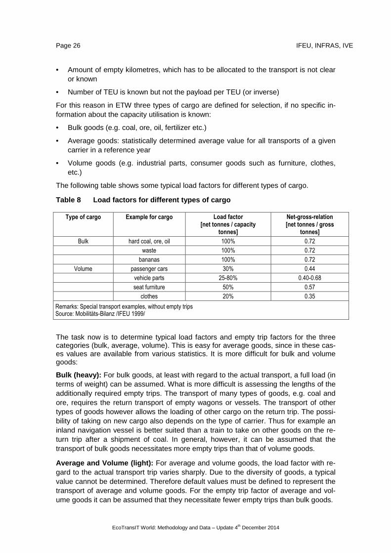
For this reason in ETW three types of cargo are defined for selection, if no specific in-formation about the capacity utilisation is known:
• Bulk goods (e.g. coal, ore, oil, fertilizer etc.)
• Average goods: statistically determined average value for all transports of a given carrier in a reference year
• Volume goods (e.g. industrial parts, consumer goods such as furniture, clothes, etc.)
The following table shows some typical load factors for different types of cargo.
Table 8 Load factors for different types of cargo
Type of cargo Example for cargo Load factor [net tonnes / capacity
tonnes]
Net-gross-relation [net tonnes / gross
tonnes]
Bulk hard coal, ore, oil 100% 0.72
waste 100% 0.72
bananas 100% 0.72
Volume passenger cars 30% 0.44
vehicle parts 25-80% 0.40-0.68
seat furniture 50% 0.57
clothes 20% 0.35
Remarks: Special transport examples, without empty trips Source: Mobilitäts-Bilanz /IFEU 1999/
The task now is to determine typical load factors and empty trip factors for the three categories (bulk, average, volume). This is easy for average goods, since in these cas-es values are available from various statistics. It is more difficult for bulk and volume goods:
Bulk (heavy): For bulk goods, at least with regard to the actual transport, a full load (in terms of weight) can be assumed. What is more difficult is assessing the lengths of the additionally required empty trips. The transport of many types of goods, e.g. coal and ore, requires the return transport of empty wagons or vessels. The transport of other types of goods however allows the loading of other cargo on the return trip. The possi-bility of taking on new cargo also depends on the type of carrier. Thus for example an inland navigation vessel is better suited than a train to take on other goods on the re-turn trip after a shipment of coal. In general, however, it can be assumed that the transport of bulk goods necessitates more empty trips than that of volume goods.
Average and Volume (light): For average and volume goods, the load factor with re-gard to the actual transport trip varies sharply. Due to the diversity of goods, a typical value cannot be determined. Therefore default values must be defined to represent the transport of average and volume goods. For the empty trip factor of average and vol-ume goods it can be assumed that they necessitate fewer empty trips than bulk goods.

IFEU, INFRAS, IVE Page 27
EcoTransIT World: Methodology and Data – Update 4th December 2014
The share of additional empty trips depends not only on the cargo specification but also to a large extent on the logistical organisation, the specific characteristics of the carri-ers and their flexibility. An evaluation and quantification of the technical and logistic characteristics of the transport carriers is not possible. We use the statistical averages for the “average cargo” and estimate an average load factor and the share of empty vehicle-km for bulk and volume goods.
Capacity utilisation of containerized sea and inter modal transport: For container-ized sea transport the basis for calculating emissions is the number of container spac-es occupied on a vessel. The second important information then is the net-weight of the cargo carried in one container. The bulk, average and volume goods have been translated into freight loads of one TEU. The net weight of a fully loaded container reaches at maximum 16.1 tonnes per TEU, corresponding to 100 % load. In accord-ance with the Clean Cargo Working Group (CCWG) the net weight of average goods is defined at 10.0 tonnes per TEU [CCWG 2014]. It is assumed that the net weights of volume and bulk goods are 6.0 respectively 14.5 tonnes per TEU. For intermodal transport – the continuing of transport on land-based vehicles in containers – the weight of the container is added to the net weight of the cargo. Table 9 provides the values used in ETW as well as the formula for calculating cargo loads in containers. For more details see appendix chapter 0.
Table 9 Weight of TEU for different types of cargo
Container [tonnes /TEU]
Net weight ([tonnes/TEU]
Total weight [tonnes/TEU]
Bulk 2.00 14.50 16.50
Average 1.95 10.00 11.95
Volume 1.90 6.00 7.90
Sources: CCWG 2014; assumptions ETW.
Capacity utilisation of road and rail transport for different cargo types
The average load factor in long distance road transport with heavy trucks was about 55 % in Germany in 2013 /KBA 2013/ and 58% in 2001 /KBA 2002/. These values also include empty vehicle-km. The share of additional empty vehicle-km in road traffic was about 11 % in 2013 and 17 % in 2001). The average load for all trips (loaded and emp-ty) was about 50 % in 2013 and 2001. The share of empty vehicle-km in France was similar to Germany in 1996 (/Kessel und Partner 1998/).
The load factor for the “average cargo” of different railway companies are in a range of about 0.5 net-tonnes per gross-tonne /Railway companies 2002a/. For dedicated freight transports the value range between 0.3 and 0.66 net-tonnes per gross-tonne /DB Schenker 2012, SNCF Geodis 2012/. According to /Kessel und Partner 1998/ Deutsche Bahn AG (DB AG) the share of additional empty vehicle-km was 44 % in 1996. This can be explained by a high share of bulk commodities in railway transport and a relatively high share of specialized rail: cars. The share of additional empty trips for dedicated trains ranges from 20 % to 100 % (see Table 10).
IFEU calculations have been carried out for a specific train configuration, based on the assumption of an average load factor of 0.5 net-tonnes per gross tonne. It can be con-cluded that the share of empty vehicle-km in long distance transport is still significantly

Page 28 IFEU, INFRAS, IVE
EcoTransIT World: Methodology and Data – Update 4th December 2014
higher for rail compared to road transport.
The additional empty vehicle-km for railways can be partly attributed to characteristics of the transported goods. Therefore we presume smaller differences for bulk and vol-ume goods and make the following assumptions:
• The full load is achieved for the loaded vehicle-km with bulk goods. Additional empty vehicle-km is estimated in the range of 60 % for road and 80 % for rail transport.
• The weight related load factor for the loaded vehicle-km with volume goods is es-timated in the range of 30 % for road and rail transport. The empty trip factor is es-timated to be 10 % for road transport and 20 % for rail transport.
These assumptions take into account the higher flexibility of road transport as well as the general suitability of the carrier for other goods on the return transport.
For railway transport of dedicated cargo average load factors and empty trip factors come from transport statistics of major railway companies /DB Schenker 2012, SNCF Geodis 2012/.
All assumptions and average values used in ETW as default are summarized in Table 10.
Table 10 Capacity utilisation of road and rail tran sport for different types of cargo
Load factor LFNC
Empty trip factor ET
Capacity utilisation CUNC
Relation Nt/Gt CUNG
Train wagon General cargo
Bulk 100% 80% 56% 0.60
Average 60% 50% 40% 0.52
Volume 30% 20% 25% 0.40
Dedicated cargo
Car 85 % 50 % 57 % 0,30
Chemistry 100 % 100 % 50 % 0,53
Container 50 % 20 % 41 % 0,56
Coal and steel 100 % 100 % 50 % 0,56
Building materials 100 % 100 % 50 % 0,55
Manufactured products 75 % 60 % 47 % 0,52
Cereals 100 % 60 % 63 % 0,66
Truck
Bulk 100% 60% 63%
Average 60% 20% 50%
Volume 30% 10% 27%
Source: DB Schenker, SNCF Geodis, IFEU estimations
Capacity utilisation for container transport on roa d and rail
ETW enables the possibility to define a value for t/TEU. At the website this value is active if a container transport (freight unit TEU) is selected. In this case the load factor

IFEU, INFRAS, IVE Page 29
EcoTransIT World: Methodology and Data – Update 4th December 2014
for trucks and trains will be calculated automatically.
The corresponding formula for the truck is
LFTruck = (Containerbrutto * Container amountvehicle) / payload capacity truck
The gross weight of a container is the sum of net weight [t/TEU] and the container weight itself (compare Table 9). The maximum payload of a truck is declared within Table 7.
At trains the load factor will only be calculated for container trains. The corresponding formula for the trains is
LFContainer Train = (Container brutto * Container amount wagon) / payload capacity container wagon
The gross weight of a container is the sum of net weight [t/TEU] and the container weight itself (compare Table 9). The payload capacity [tonnes] of a container wagon is declared within Table 7.
Capacity utilisation of ocean-going vessels for dif ferent cargo types
Capacity utilisation for sea transport is differentiated per vessel type. Most significantly is the differentiation between bulk vessels and container vessels, which operate in scheduled services. The operational cycle of both transport services lead to specific vessel utilisation factors. Furthermore, the vessel load factor and the empty trip factor have been combined to the vessel capacity factor for reasons to avoid common mis-takes. It is assumed that performance of ocean-going vessels sailing under laden con-ditions (when carrying cargo) and ballast conditions (when empty) are relatively similar. The cargo weight of ocean-going vessels only influence the energy consumption to a minor extend, in particular compared to other modes of transport. Reasons are the need to reach a certain draft for safety reasons, which is adjusted by taking up or dis-charging ballast water and the dominance of other factors that determine the vessels’ fuel consumption, namely wave and wind resistance. Wave resistance exponentially increases with speed, which makes speed as one of the most important parameters. While for bulk carriers the difference between laden and ballast conditions might be recognisable, it should be acknowledged that container carriers carry cargo in all direc-tions and always perform with both cargo and ballast water loaded. For container ves-sels the nominal TEU capacity (maximum number of TEU units on-board) is considered the full load.
The combined vessel utilisation for bulk and general cargo vessels is assumed to be between 48 % and 61 % and follows the IMO assumptions /IMO 2009/. Bulk cargo vessels usually operate in single trades, meaning from port to port. In broad terms, one leg is full whereas the following leg is empty in normal cases. However, cycles can be multi-angular and sometimes opportunities to carry cargo in both directions may exist. The utilisation factors are listed in Table 11.

Page 30 IFEU, INFRAS, IVE
EcoTransIT World: Methodology and Data – Update 4th December 2014
Table 11 Capacity utilisation of sea transport for different types of ships
Vessel types
Trade lane / size class
Capacity utilisation
factor
BC (dry, liquid and GC) Suez trade 49% Transatlantic trade 55% Transpacific trade 53% Panama trade 55% Other global trade 56% Intra-continental trade 57% Great lake 58% Bulk carrier dry Feeder (5,000 - 15,000 dwt) 60% Handysize (15,000 - 35,000 dwt) 56% Handymax (35'000 - 60,000 dwt) 55% Panamax (60,000 - 80,000 dwt) 55% Aframax (80'000 - 120,000 dwt) 55% Suezmax (120,000 - 200,000 dwt) 50% Bulk carrier liquid Feeder (5,000 - 15,000 dwt) 52% Handysize (15,000 - 35,000 dwt) 61% Handymax (35'000 - 60,000 dwt) 59% Panamax (60,000 - 80,000 dwt) 53% Aframax (80'000 - 120,000 dwt) 49% Suezmax (120,000 - 200,000 dwt) 48% VLOC(+) (>200,000 dwt) 48% General cargo (GC) All trades, all size classes 60% Container vessel (CC) All trades, all size classes 70% Ferry / RoRo vessels All trades, all size classes 70% Note: BC = bulk carrier, GC = general cargo, CC = container cargo vessel. Sources: Seum 2010; IMO 2009; CCWG 2014.
Ships in liner service (i.e. container vessels and car carriers) usually call at multiple ports in the sourcing region and then multiple ports in the destination region (see Fig-ure 4). It is also common that the route is chosen to optimize the cargo space utilisation according to the import and export flows. For example, on the US West Coast a par-ticular pattern exists where vessels from Asia generally have their first call at the ports of Los Angeles or Long Beach to unload import consumer goods and then travel rela-tively empty up the Western Coast to the Ports of Oakland and other ports, from which then major food exports leave the United States. Combined utilisation factors for con-tainer vessels (net load of container spaces on vessels and empty returns) used in ETW is 70% independent of vehicle sizes and trade lanes (see Table 11). This figure equates to the utilisation factor for container ships used by the Second IMO GHG Study 2009 /IMO 2009/. The Clean Cargo Working Group recommends alike to use this value to recalculate their CO2 emission values of the container ships considering real utilisation factors /CCWG 2014/.

IFEU, INFRAS, IVE Page 31
EcoTransIT World: Methodology and Data – Update 4th December 2014
Figure 4: Sample Asia North America Trade Lane by H apag Lloyd AG 2
Capacity utilisation of inland vessels for differen t cargo types
The methodological approach to inland vessels is in line with the approach for calculat-ing ocean-going vessels. The cargo load factor and the empty trip factor are also com-bined to a vessel utilisation factor.
The dominant cargo with inland vessels is bulk cargo, although the transport of con-tainerized cargo has been increasing. For bulk cargo on inland vessels, the principle needed to reposition the inland vessel applies. Thus, empty return trips of around 50 % of the time can be assumed. However, no good data is available from the industry. Therefore, it was assumed that the vessel utilisation is 45 % for all bulk inland vessels smaller class VIb (e.g. river Main). Class Va RoRo and class VIb vessels were estimat-ed to have a 60 % vessel utilisation.
Container inland vessels were assumed to have a vessel utilisation of 70 % in analogy with the average container vessel utilisation cited in /IMO 2009/. This reflects less than full loads of containers as well as the better opportunity of container vessels to find carriage for return trips in comparison with bulk inland vessels.
Capacity utilisation of air freight
Since mainly high value volume or perishable goods are shipped by air freight, the permissible maximum weight is limited. Therefore only the volume goods category is considered; other types of goods (bulk, average) are excluded. Table 12 shows the capacity utilisation differentiated by short, medium and long haul (definition see Table 12) /DECC 2014; Lufthansa 2014; EUROCONTROL 2013b; ICAO 2012/. Similar to container ships the utilisation factor refers to the whole round trip of the airplane and includes legs with higher and lower load factors as well as empty trips (like ferry 2 Internet Site from 01/10/2014.

Page 32 IFEU, INFRAS, IVE
EcoTransIT World: Methodology and Data – Update 4th December 2014
flights). The utilisation factors used for airplane by ETW are included in Table 12. The values for freight refer to the maximum weight which can be transported by freighter or passenger aircraft. The utilisation factors for passenger presented in Table 12 pro-vide information about the seats sold. The latter is used for the allocation of energy consumption and emissions between air cargo and passenger (see chapter 5.5).
Table 12 Capacity utilisation of freight and passen ger for aircrafts
Freight
(freighters and pas-senger aircrafts
Passenger (only passenger
aircrafts)
Short haul (up to 1,000 km) 50% 65%
Medium haul (1,001 – 3,700 km) 70% 70%
Long haul (more than 3,700 km) 70% 80%
Sources: DECC 2014; Lufthansa 2014; EUROCONTROL 2013b; ICAO 2013.
3.3 Basic calculation rules
In ETW the total energy consumption and emissions of each transport mode are calcu-lated for vehicle usage (TTW) and the upstream process (WTT; see chapter 2.3). Thus several calculation steps are necessary:
1. Final energy consumption (TTW energy consumption) per net tonne-km
2. Energy related vehicle emissions per net tonne km (TTW)
3. Combustion related vehicle emissions per net tonne km (TTW)
4. Energy consumption and emission factors for upstream process per net tonne km (WTT)
5. Total energy consumption and total emissions per transport (WTW)
The following subchapters describe the basic calculation rules for each step. For each transport mode the calculation methodology can differ slightly. More information about special calculation rules and the database are given in Chapter 5.
3.3.1 Final energy consumption per net tonne km (TT W)
The principal calculation rule for the calculation of final energy consumption is
Final energy consumption per net tonne km = * specific energy consumption of vehicle or vessel per km
/ (payload capacity of vehicle or vessel * capacity utilisation of vehicle or vessel)
The corresponding formula is
ECFtkm,i = ECFkm,i, / (CP *CU)

IFEU, INFRAS, IVE Page 33
EcoTransIT World: Methodology and Data – Update 4th December 2014
Abbr. Definition Unit
ECFtkm,i Final energy consumption (TTW) per net tonne km for each energy carrier i [MJ/tkm]
i Index for energy carrier (e.g. diesel, electricity, HFO)
ECFkm,i, Final energy consumption of vehicle or vessel per km; normally depends on mass related capacity utilisation
[MJ/km]
CP Payload capacity [tonne]
CU Capacity utilisation [%]
Explanations:
• Final energy consumption (TTW) is the most important key figure for the calculation of total energy consumption and energy related emissions of transport. For the fol-lowing calculation steps, final energy consumption must be differentiated for each energy carrier because different sets of emission factors and upstream energy con-sumption have to be considered for each energy carrier.
• Final energy consumption depends on various factors (see chapter 3.1). In particu-lar, it should be pointed out that e.g. final energy consumption per kilometre for trucks also depends on capacity utilisation and thus the denominator of the formula.
• As mentioned in chapter 2.1, energy consumption values per tkm combine the steps calculation of energy consumption on a vehicle, train, vessels or airplanes basis and allocation of energy consumption to one single shipment. In the Europe-an standard EN 16258 these steps are described consecutively. Nevertheless the steps can be done in an integrated manner. To fulfil the requirements of EN 16258 it is more important that the VOS is defined in accordance with the European standard and considers the entire round-trips including empty runs. ETW fulfils these requirements without exceptions.
• The formula above refers to a typical case, which is usual for trucks (final energy consumption per vehicle km). For other modes, the calculation methodology can be slightly different (see explanations in chapter 5). However, for all modes the same relevant parameters (final energy consumption of vehicle/vessel, payload capacity and capacity utilisation) are needed.
3.3.2 Energy related emissions per net tonne km (TT W)
The principle calculation rule for the calculation of energy related vehicle emissions is
TTW Vehicle emissions per net tonne-km = specific energy consumption of vehicle or vessel per net tonne km
* energy related vehicle emission factor per energy carrier
The corresponding formula is
EMVtkm,i = ECFtkm,i, * EMVEC,i

Page 34 IFEU, INFRAS, IVE
EcoTransIT World: Methodology and Data – Update 4th December 2014
Abbr. Definition Unit
EMVtkm,i Vehicle emissions (TTW) per net tonne km for each energy carrier i [g/tkm]
i Index for energy carrier (e.g. diesel, electricity, HFO)
ECFtkm,i Final energy consumption (TTW) per net tonne km for each energy carrier i [MJ/tkm]
EMVEC,i Energy related vehicle emission factor (TTW) for each energy carrier i [g/MJ]
Explanations:
• The formula is used for all emission components which are directly correlated to final energy consumption (TTW CO2 and SO2 emissions) and for combustion relat-ed emissions of fuel driven trains and ships (see chapter 5.2 to 5.4). The formula is also used for the calculation of standardized TTW energy consumptions in MJ. In this case the energy related energy factors are used (e.g. MJ per litre diesel). To fulfil the requirements of EN 16258 the energy factors of the European standard EN 16258 are used by ETW (see chapter 6.1 in the annex).
• Based on the European standard the CO2 equivalents are also calculated by multi-plication of the TTW energy consumption with energy related TTW emission factors (e.g. kg CO2e per litre diesel). For this calculation step the emission factors respec-tively conversion factors of the European standard EN 16258 are used without changes. The used values are documented in chapter 6.1 in the annex).
• The CO2 emission factors used by ETW (e.g. kg CO2/litre diesel) are based on the same sources like the CO2 equivalent emission factors included in the European standard EN 16258. Therefore CO2 emission quantifications can’t be in accordance with EN 16258 since only CO2 equivalent calculations are required by European standard. Nevertheless ETW allows the calculation of CO2 emissions based on the same methodology and the same data sources as the European standard EN 16258.
3.3.3 Combustion related emissions per net tonne km (TTW)
The principal calculation rule for the calculation of TTW NOx, NMHC and particles emissions (so called combustion related emissions) is
TTW Emissions per net tonne km = * specific emission factor of vehicle or vessel per km
/ (payload capacity of vehicle or vessel * capacity utilisation of vehicle or vessel)
The corresponding formula is
EMVtkm,i = EMVkm,i, / (CP *CU)

IFEU, INFRAS, IVE Page 35
EcoTransIT World: Methodology and Data – Update 4th December 2014
Abbr. Definition Unit
EMVtkm,i Vehicle emissions consumption (TTW) per net tonne km for each energy carrier i [g/tkm]
i Index for energy carrier (e.g. diesel, electricity, HFO)
EMVkm,i, Combustion related vehicle emission factor (TTW) of vehicle or vessel per km; nor-mally depends on mass related capacity utilisation
[g/km]
CP Payload capacity [tonne]
CU Capacity utilisation [%]
Explanations:
• The formula is used for vehicle/vessel emissions of truck and aircraft operation.
• For rail and ship combustion related emission factors are derived from emissions per engine work, not per vehicle-km. Thus they are expressed as energy related emission factors and calculated with the formula in chapter 3.3.2.
3.3.4 Upstream energy consumption and emissions per net tonne km (WTT)
The principle calculation rule for the calculation of vehicle emissions is
WTT Upstream energy consumption or emissions per net tonne-km = specific energy consumption of vehicle or vessel per net tonne km
* energy related upstream energy or emission factor per energy carrier
The corresponding formulas are
EMUtkm,i = ECFtkm,i, * EMUEC,I
ECUtkm,i = ECFtkm,i, * ECUEC,i
Abbr. Definition Unit
EMUtkm,i Upstream emissions (WTT) for each energy carrier i [g/tkm]
ECUtkm,i Upstream energy consumption (WTT) for each energy carrier i [MJ/tkm]
i Index for energy carrier (e.g. diesel, electricity, HS)
ECFtkm,i Final energy consumption (TTW) per net tonne km for each energy carrier i [MJ/tkm]
EMUEC,i Energy related upstream emission factor (WTT) for each energy carrier i [g/MJ]
ECUEC,i Energy related upstream energy consumption (WTT) for each energy carrier i [MJ/MJ]
Explanations:
• Formulas for upstream energy consumption and emissions are equal, but have different units.
• Formulas are equal for all transport modes; upstream energy consumption and emission factors used in ETW are explained in chapter 5.5.5.
• For the calculation of WTT energy and WTT CO2 equivalent the emission factors of the new European standard are used for ETW. Only for electricity EN 16258

Page 36 IFEU, INFRAS, IVE
EcoTransIT World: Methodology and Data – Update 4th December 2014
doesn’t provide emission factors. Therefore ETW calculates own emission factors for electricity in accordance to the European standard. The methodology as well as used values is documented in the chapters 5.5.5 and 6.1.
3.3.5 Total energy consumption and emissions of tra nsport (WTW)
The principal calculation rule for the calculation of vehicle emissions is
WTW energy consumption or emissions per transport = Transport Distance
* mass of freight transported * (TTW energy consumption or vehicle emissions per net tonne km
+ WTT energy consumption or emissions per net tonne km)
The corresponding formulas are
EMTi = Di* M* (EMVtkm,i + EMUtkm,i)
ECTi = Di* M* (ECFtkm,i + ECUtkm,i)
Abbr. Definition Unit
EMTi WTW emissions of transport [kg
ECTi WTW energy consumption of transport [MJ]
Di Distance of transport performed for each energy carrier i [km]
M Mass of freight transported [net tonne]
EMVtkm,i TTW Vehicle emissions for each energy carrier i [g/tkm]
ECFtkm,i TTW energy consumption for each energy carrier i [MJ/tkm]
EMUtkm,i WTT (upstream) emission factors for each energy carrier i [g/tkm]
ECUtkm,i WTT (upstream) energy consumption for each energy carrier i [MJ/tkm]
i Index for energy carrier (e.g. diesel, electricity, HS)
Explanations:
• Transport distance is a result of the routing algorithm of ETW (see chapter 4).
• WTW energy consumption and emissions also depend on routing (e.g. road cate-gories, electrification of railway line, gradient, distance for airplanes). This correla-tion is not shown as variable index in the formulas due to better readability.
• Mass of freight is either directly given by the client or recalculated from number of TEU, if TEU is selected as input parameter in the extended input mode of ETW.
• Using the formula described above for the calculation of WTW energy consumption and WTW CO2 equivalent emissions of transport services fulfils the requirements of EN 16258. Therefore the methodology is in accordance with the European standard.
3.4 Basic allocation rules
ETW is a tool which takes the perspective of a shipper – the owner of a freight that has to be transported – that want to estimate the emissions associated with a particular

IFEU, INFRAS, IVE Page 37
EcoTransIT World: Methodology and Data – Update 4th December 2014
transport activity or a set of different transport options. Within the European standard EN 16258 the transport activity is also called as transport service . But ETW may be also used by carriers – the operators and responsible parties for operating vehicles and vessels – to estimate emissions for example for benchmarking. The calculation follows principles of life cycle assessments (LCA) and carbon footprints.
The major rule is that the shipper (freight owner) and carrier take responsibility for the vessel utilisation factor that is averaged over the entire journey, from the starting point to the destination as well as the return trip or the entire loop respectively. This alloca-tion rule has been common practice for land-based transports in LCA calculations and is applied also to waterborne and airborne freight. Thus, even if a shipper may fill a tanker to its capacity, he also needs to take responsibility for the empty return trip which would not have taken place without the loaded trip in the first place. Therefore, a shipper in this case will have to apply a 50 % average load over the entire return jour-ney. This fundamental ecological principle considered by ETW is also a general re-quirement from EN 16258. Only by considering the average load factor for the entire journey (as vehicle operation system named by the EN 16258) CO2 calculations fulfil the European standard.
Similarly, other directional and trade-specific deviations, such as higher emissions from head winds (aviation), sea currents (ocean shipping) and from river currents (inland shipping) are omitted. These effects, which are both positive and negative depending on the direction of transport, cancel one another out and the shipper needs to take re-sponsibility for the average emissions. It is the purpose of ETW to provide the possibil-ity of modal comparisons and calculations of transport services consisting of different transport modes. This also requires that all transport modes are equally treated. Thus, average freight utilisation and average emissions without directional deviations are generally considered.
In ETW energy and emissions are calculated for transport services of a certain amount of a homogeneous freight (one special freight type) for a transport relation with one or several legs. For each leg one type of transport vessel or vehicle can be selected. These specifications determine all parameters needed for the calculation:
• Freight type: Load factor and empty trip factor (can also be user-defined in the extended input mode)
• Vehicle/vessel type: Payload capacity (mass related), final energy consump-tion and emission factors.
• Transport relation: road type, gradient, country/region specific emission fac-tors.
For the calculation algorithm it is not relevant whether the freight occupies a part of a vehicle/vessel or one or several vessels. Energy consumption and emissions are al-ways calculated based on the capacity utilisation of selected freight type and the cor-responding specific energy consumption of the vessel. These assumptions avoid the need of different allocation rules for transports with different freight types in the same vehicle, vessel or train. Therefore no special allocation rules are needed for road and rail transport. This approach is also in accordance with EN 16258. The European standard requires that the same allocation rules shall be used for the same vehicles.

Page 38 IFEU, INFRAS, IVE
EcoTransIT World: Methodology and Data – Update 4th December 2014
For passenger ferries and passenger aircrafts with simultaneous passenger and freight transport (belly freight) allocation rules for the differentiation of passenger and freight transport are necessary. These rules are explained in the related chapters. The approaches selected for ETW are also in line with the requirements of the European standard EN 16258.

IFEU, INFRAS, IVE Page 39
EcoTransIT World: Methodology and Data – Update 4th December 2014
4 Routing of transports
4.1 General
For the calculation of energy consumption and environmental impacts ETW has to de-termine the route between origin and destination for each selected traffic type. There-fore ETW uses a huge GIS database including worldwide locations and networks for streets, railways, aviation, sea and inland waterways.
Figure 5 Networks of ETW
Name Type Attributes
Road Network Road classes, Ferry, Country code
Railway Network Electrification, European freight corridors, Ferry, Country code
Ocean shipping Network Cannel
Inland waterways Network Water classes, Country code
Air routing Direct No network needed, routing on the base of the great circle formula between the airport locations
Figure 6 Locations of ETW
Name Type Attributes
City and District names Location City name, District name, Country, Location classes, (Translations)
Zip codes Location Country code/ Zip code, City name, Country code
Stations (UIC-Codes) Location Station name, UIC-Code/ station code, Country code
UN-/LOCodes Location UN-/LOCode, Location name, Country Code, Ports classes, Inland locations
Airports (IATA-Codes) Location IATA-Code, Airport name, Country code, Airport classes
Longitude/ Latitude Location No location layer or attributes are needed
4.2 Routing with resistances
Depending on the transport type and the individual settings ETW routes the shortest way in consideration of network attributes (resistances). These network attributes are e.g. street classes at the road routing or cannels at the ocean routing. If there is a mo-torway between the origin and the destination the truck will probably use it on its route according to the principle of “always using the path of lowest resistance” defined within ETW. Technically, a motorway has a much lower resistance (factor 1.0) than a city-street (factor 5). Thus, a route on a highway has to be more than five times as long as a city-street before the local street will be preferred. These resistances are used for almost every transport type.
4.2.1 Road network resistances
The street network is divided into different street categories, which are used for the routing as resistances.

Page 40 IFEU, INFRAS, IVE
EcoTransIT World: Methodology and Data – Update 4th December 2014
Table 13 Resistance of street categories
Street category Resistance
Highway (Category 0) 1.0
Large country road (Category 1) 1.3
Small country road (Category 2) 1.5
Large urban road (Category 3) 1.67
Urban road (Category 4) 2.5
Small urban road (Category 5-7) 3.33
Additionally, there are ferry routes within the street network. These ferry routes work like virtual roads where the whole truck is put on the ferry. ETW has different resistanc-es for ferry routes included.
Table 14 Resistance for ferries in the road network
Ferry handling Resistance
Standard 5.0
Preferred 1.0
Avoid 100.0
4.2.2 Railway network resistances
Railways have the attributes of electrified or diesel line and dedicated freight corridor. If an electrified train is selected, diesel lines can also be used but they get a higher re-sistance than electrified lines. This is needed if there is no electrified line available or to circumnavigate possible data errors concerning the electrification of the railway net.
The attribute freight corridor is used as a railway highway. Lines with this attribute will be used with preference.
Table 15 Resistance for the railway network
Attribute Resistance
Freight corridor 1,0
Non freight corridor 1,8
Diesel tracks at electrified calculation 4,0
Additionally, there are ferry routes within the rail network. These routes work like virtual tracks where the whole train is put on the ferry. ETW has different resistances for ferry routes included.
Table 16 Resistance for ferries in the railway netw ork
Ferry handling Resistance
Standard 5,0
Preferred 1,0
Obstruct 100,0

IFEU, INFRAS, IVE Page 41
EcoTransIT World: Methodology and Data – Update 4th December 2014
4.3 Sea ship routing
A sea ship normally takes the direct and shortest way between two sea-ports3, har-bours, although it often deviates slightly from direct routes due to weather and ocean drift conditions. Therefore, a very large and flexible network is needed. The solution to this is a huge amount of so-called sea nodes, which were placed everywhere in the world close to the coast or around islands. Every sea node is connected with every other sea node as long it does not cross a country side. The result of these connec-tions is a routable sea network.
Figure 7 Sea network area around Korea /IVE mbh 201 4/
Canals and certain sea bottlenecks, e.g. the Kattegat strait, are considered as size restricted passages (by draft, length and width) in this network. Every canal and bottle-neck has the attributes of “maximum dead weight tonnes” (DWT) and “maximum TEU capacity” for vessels and is limited to for the classified ship types.
The Suez, Panama and Kiel canals are also included as restricted canals in the ETW sea ship network. Whereas through the Suez Canal even the largest container vessel can pass, the bulk carriers are restricted to 200,000 DWT, which represents the Suez-Max class ships. The Panama-Canal is restricted to bulk carriers up to 80,000 DWT
3 Container vessels and car carriers often operate as liner traffic and call at multiple ports
on a scheduled route. The routing differs from ocean carrier to ocean carrier and may lead to longer distances between a loading and discharging port. Those schedules are not considered in EcoTransIT World today.

Page 42 IFEU, INFRAS, IVE
EcoTransIT World: Methodology and Data – Update 4th December 2014
and container carriers up to 4,700 TEU capacity, the Kiel Canal is restricted to bulk carriers up to 60,000 DWT and container vessels up to 3500 TEU capacity. Additional-ly, there are small sea areas, like the Kattegat strait between Denmark and Sweden and the entrance to the Great Lakes, next to Montreal, Canada, which are handled as canals and restricted as well (80000 DWT and 4700 TEU for the Kattegat and 60000 DWT and 3500 TEU for the entrance to the Great Lakes).
Ports are considered if they have significant marine traffic. Every port is located and allocated to a specific geographic region (compare Figure 3). On the base of the com-bination of start and destination location enables the determination of the respective trade lane. For example, on the transatlantic trade, connecting Europe with North America, ETW selects bulk vessels between 35000 and 80000 DWT and container vessels with a TEU capacity of 2000 to 4700 TEU as default ships. If the starting point and destination belong to the same geographic region, an “intra-continental” vessel size is selected. Within Europe an “intra-continental Europe” vessel size is used and if the origin and destination harbour is within the SECA zone (Baltic Sea) an “intra-continental Europe SECA” vessel size will be applied.
4.3.1 Routing inland waterway ship
The inland waterway network has an attribute for inland waterway class. Depending on the ship size waterways and the respective waterway class a waterway can be used or not. Whereas the euro barge can only be used on inland waterways above the class IV (standard European inland waterway), bigger barges need at least waterway class V or higher. Compare also with chapter 5.4.1.
4.4 Aviation routing
In ETW a validation exists if the selected airport is suitable for the flight (compare chap-ter 4.5). Therefore all airports are categorized. Depending of the airport category desti-nations of different distances can be reached.
Table 17 Airport size and reach
Airport size Reach
Big size over 5000 km
Middle size Over 5000 km (but not overseas)
Small size maximum 5000 km
Very small size maximum 2500 km
After the selection of the airport, EcoTransIT calculates the distance between the two airports. If the closest airport allows the distance of the flight, it will be selected. If the limit is exceeded, the next bigger airport will be suggested and so on.
The air routing is not based on a network. The calculation of the flight distance uses the Great Circle Distance (GCD). By definition it is the shortest distance between two points on the surface of a sphere. GCD is calculated by using the geographical coor-dinates of the two airports which are selected by the EcoTransIT user.
However, the real flight path is longer than the GCD due to departure and arrival pro-cedures, stacking, adverse weather conditions, restricted or congested airspace

IFEU, INFRAS, IVE Page 43
EcoTransIT World: Methodology and Data – Update 4th December 2014
/Kettunen et al. 2005, Gulding et al. 2009, Reynolds 2009/. Therefore the European standard EN 16258 as well as the European Emission Trading System (ETS) pre-scribed adding a blanket supplement of 95 km to the GCD for each leg of flight. This approach is also adopted by ETW. Based on this requirement the real flight distance is calculated by using the following formula:
Real flight distance = GCD + 95 km
In ETW airplanes have a maximum reachable distance (so called maximum design range). If the distance between the airports exceeds this distance ETW cannot calcu-late the emissions for this specific airplane and the error message “Route not found” will be applied. To avoid this error the user has the possibilities to insert a stop-over as via point in the transport chain or to calculate with a hybrid plane.
A hybrid airplane is a mixture of the belly freight airplane B747-400 and the freighter B747-400F (see chapter 5.5). The maximum design range of this hybrid plane is 8,230 kilometres. If the flight distance exceeds this range an additional virtual stopover is au-tomatically included for each 8,230 kilometres. If stopovers are considered for each of the legs a blanket supplement of 95 km is added to the GCD.
4.5 Determination of transport points within combin ed transport chains
The routing is available on the different networks for road, railway, ocean, inland wa-terways and air routes. Depending on the selected mode, ETW determines a route on the respective transport type network.
All networks are connected with so-called transfer points. These transfer points ena-bles the change of a network. Thus it is possible to calculate complex transport chains with ETW.
Furthermore ETW has an algorithm to determine the probable transfer point of the transport chain. This is needed if the user wants to calculate a sea shipping transport and defines zip codes as origin and destination (instead of two UN-/LOCodes for the ports). In this case, ETW has to determine the closest situated suitable ports to the origin and destination. After the determination of these transfer points and the routing, algorithm locates the routes (in the normal case on the street network) to these transfer point ports. Finally, the main routing between the two ports will be applied on the base of the ocean sea shipping network.
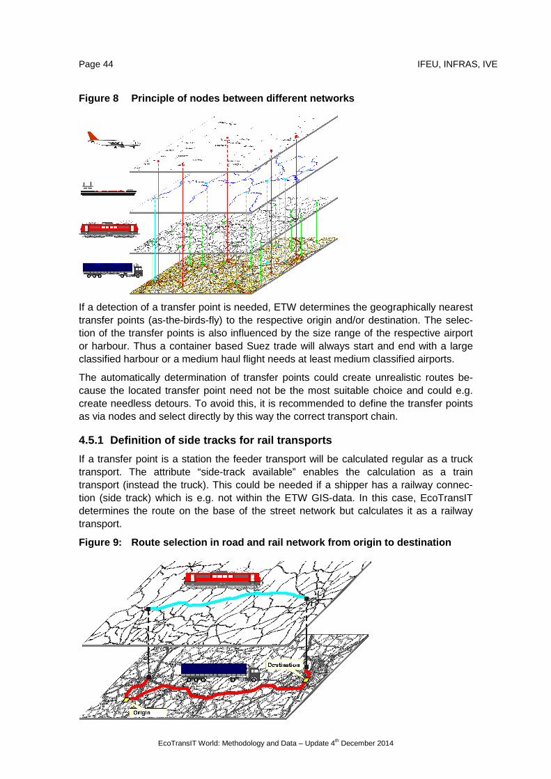
Page 44 IFEU, INFRAS, IVE
EcoTransIT World: Methodology and Data – Update 4th December 2014
Figure 8 Principle of nodes between different netwo rks
If a detection of a transfer point is needed, ETW determines the geographically nearest transfer points (as-the-birds-fly) to the respective origin and/or destination. The selec-tion of the transfer points is also influenced by the size range of the respective airport or harbour. Thus a container based Suez trade will always start and end with a large classified harbour or a medium haul flight needs at least medium classified airports.
The automatically determination of transfer points could create unrealistic routes be-cause the located transfer point need not be the most suitable choice and could e.g. create needless detours. To avoid this, it is recommended to define the transfer points as via nodes and select directly by this way the correct transport chain.
4.5.1 Definition of side tracks for rail transports
If a transfer point is a station the feeder transport will be calculated regular as a truck transport. The attribute “side-track available” enables the calculation as a train transport (instead the truck). This could be needed if a shipper has a railway connec-tion (side track) which is e.g. not within the ETW GIS-data. In this case, EcoTransIT determines the route on the base of the street network but calculates it as a railway transport.
Figure 9: Route selection in road and rail network from origin to destination

IFEU, INFRAS, IVE Page 45
EcoTransIT World: Methodology and Data – Update 4th December 2014
5 Methodology and environmental data for each trans port mode
Within the next chapters the methodology for the calculation of energy consumption and emissions of freight transport as well as the data sources used are presented for each mode of transport in detail. The methodology for the calculation of energy con-sumption and CO2 equivalent emissions are in accordance with the European standard EN 16258. As required by the standard all used data sources and allocation methodol-ogies are documented in the following chapters.
5.1 Road transport
5.1.1 Classification of truck types
ETW is focused on international long distance transports. These are typically accom-plished using truck trains and articulated trucks. Normally, the maximum gross tonne weight of trucks is limited, e.g. 40 tonnes in most European countries, 60 tonnes in Sweden and Finland and 80,000lbs in the United States on highways. For feeding or special transports, other truck types are used. In ETW, the gross weight classes for all vehicle sizes used for cargo transport are as follows:
Table 18 Truck size classes in ETW
EU/Japan EPA
LDV <=3.5t
Truck <=7.5t Truck <=16,000lbs
Truck >7.5-12t Truck >16,000-26,000lbs
Truck >12-20t Truck >26,000-44,000lbs
Truck >20-26t Truck >44,000-60,000lbs
Truck >26-40t Truck >60,000-80,000lbs
Truck >40-60t Truck >80,000lbs
Besides the vehicle size, the emission standard of the vehicle is an important criterion for the emissions of the vehicle. In European transport, different standards (EURO I -EURO VI) are used. The Pre-EURO I-standard is no longer relevant for most long dis-tance transports, and therefore it is not included.
The European emission standard is used in most countries worldwide for emission leg-islation. Other relevant standards are the US EPA emission regulations and the Japa-nese standards. The following table shows the emission standards used in ETW.
Table 19 Emission standards in ETW
EU EPA Japan
Euro-I (1992) EPA 1994 JP 1994
Euro-II (1996) EPA 1998 JP 1997
Euro-III (2000) EPA 2004 JP 2003
Euro-IV (2005) EPA 2007 JP 2005
Euro-V (2008) EPA 2010 JP 2009
Euro-VI (2013) n.a. n.a.
Page 46 IFEU, INFRAS, IVE
EcoTransIT World: Methodology and Data – Update 4th December 2014
5.1.2 Final energy consumption and vehicle emission factors (TTW)
The main sources for final energy consumption and vehicle emission factors is the “Handbook emission factors for road transport” (HBEFA) /INFRAS 2014/ for trucks with EU emission limits and the MOVES model for EPA standard /EPA 2009/. The new ver-sion of the moves model, which was published in July 2014, could not be considered in the present update of EcoTransIT due to time restrictions. Therefore all values for EPA trucks are still based on the analysis of /EPA 2009/.
The influence of the load factor is modelled according to the Handbook of Emission Factors /INFRAS 2014/. Accordingly, the fuel consumption of an empty vehicle can be 1/3 below the fuel consumption of the fully loaded vehicle. This influence can be even stronger depending on driving characteristics and the gradient.
Energy consumption and emissions also depend on the driving pattern. Two typical driving patterns, one for highway traffic and one for traffic on other (mainly extra urban) roads, are considered by ETW. Traffic on urban roads has a small fraction in long dis-tance transport and is therefore included in the other roads.
Another parameter is the gradient . Similar to rail transport, the gradient takes into ac-count country-specific factors, which represent the average topology of the country (“flat”, “hilly”, and “mountains”). IFEU and INFRAS analyses for Germany /IFEU 2002b/ and Switzerland /INFRAS 1995/ show 5-10 % higher energy consumption and emis-sions for heavy duty vehicles if the country specific gradients are taken into account. No significant differences could be determined between the countries of Germany and Switzerland. However, for these analyses, the entire traffic on all roads has been con-sidered.
The share of gradients for the different countries in international road transports can only be estimated. No adjustments will be made for the “hilly countries” such as Ger-many (and all others except the following named), while energy consumption and emissions are assumed 5 % lower for the “flat countries” (Denmark, Netherlands and Sweden) and 5 % higher for the “mountainous countries” Switzerland and Austria. For all regions outside Europe the values for “hilly” are used.
The energy and emission factors of road transport for ETW are derived from the Hand-book of Emission Factors (HBEFA 3.2) /INFRAS 2014/ for trucks with Euro standards. For the determination of values for trucks in North America several sources were ana-lysed:
• emission limit values for the EPA standard compared with the EU standard /Dieselnet 2014/
• the emission model MOVES2010 to compare emission factors and energy con-sumption of trucks by road type, registration year and size /EPA 2009/
• further statistical data (/USCB 2004/, /USDOT 2007/, /USDOE 2009/) on truck size classification, average utilisation and energy consumption
Comparison of Emission standards
A comparison of the U.S., EU and Japanese emission limit values provides insight into the potential difference between the trucks exhaust emission characteristics for these countries. (See Figure 10)

IFEU, INFRAS, IVE Page 47
EcoTransIT World: Methodology and Data – Update 4th December 2014
Figure 10 EU, Japanese and U.S. Emission Limit Valu es for Heavy Duty Diesel Vehicles by Emission Standard and Testing Procedure (without Eu-ro VI)
NOx
PM
* combined limit value of 3.38 g/kWh NMHC+NOx Source: /Dieselnet 2009/
0
1
2
3
4
5
6
7
8
Euro
I
JP
1994
EPA
1994
Euro
II
JP
1997
EPA
1998
Euro
III
JP
2003
EPA
2004*
Euro
IV
JP
2005
EPA
2007
Euro
V
JP
2009
EPA
2010
[g/k
Wh
]
Mode Test
Transient Cycle
0.0
0.1
0.2
0.3
0.4
0.5
0.6
0.7
Euro
I
JP
1994
EPA
1994
Euro
II
JP
1997
EPA
1998
Euro
III
JP
2003
EPA
2004
Euro
IV
JP
2005
EPA
2007
Euro
V
JP
2009
EPA
2010
[g/k
Wh
]
Mode Test
Transient Cycle

Page 48 IFEU, INFRAS, IVE
EcoTransIT World: Methodology and Data – Update 4th December 2014
Comparison of energy consumption and emission value s
The figure below illustrates the differences in energy consumption and emission values between EU and U.S. trucks. The data is based on the U.S. emission model MOVES and the German transport emission model TREMOD /IFEU 2005/.
Figure 11: Specific emission of heavy trucks* in 20 10 by registration year – com-parison of U.S. (MOVES) and German (TREMOD)** emiss ion models data
Diesel fuel consumption
NOx
PM
* Trucks on motorway; in DE GVW >14t; in U.S. GVW >15t (metric tonnes) ** based on previous version of /INFRAS 2010/ Sources: /IFEU 2005/; /EPA 2009/
The Handbook Emission Factors for Road Transport HBEFA /INFRAS 2014/ delivers data on specific emission and energy consumption of trucks in 2014 by emission standard, truck size and road type. Unfortunately, in the U.S. model MOVES2010 /EPA 2009/ trucks are only classified by road type, truck size and vehicle age, but not by emission standard.
To determine emission factors for U.S. trucks with a classification like in /INFRAS 20104/, we assumed that U.S. trucks in 2010 which were registered in 1994
0
10
20
30
40
50
1994 1995 1996 1997 1998 1999 2000 2001 2002 2003 2004 2005 2006 2007 2008 2009 2010
[l/1
00k
m]
MOVES2010
TREMOD4.17
0
5
10
15
20
1994 1995 1996 1997 1998 1999 2000 2001 2002 2003 2004 2005 2006 2007 2008 2009 2010
[g/k
m]
MOVES2010
TREMOD4.17
0.0
0.2
0.4
0.6
0.8
1994 1995 1996 1997 1998 1999 2000 2001 2002 2003 2004 2005 2006 2007 2008 2009 2010
[g/k
m]
MOVES2010
TREMOD4.17

IFEU, INFRAS, IVE Page 49
EcoTransIT World: Methodology and Data – Update 4th December 2014
represent the EPA1994 standard, with registration in 1998 representing EPA1998 standard etc.
A comparison with the Euro-VI standard in 2013 should be analysed in a future update of ETW, based on MOVES2014.
On the basis of these assumptions and the emission limit values we estimated the ad-justing factors, shown in the table below. Presently we have no information about ener-gy consumption for Japanese trucks. Therefore we take the energy consumption from Europe for Japanese trucks.
Table 20 Adjusting factors for derivation of energy and emissions factors for North American and Japanese trucks in ETW
Emission Standard Related to Energy NMVOC NOx PM Emission Standard Consumption
EPA 1994 Euro-I 1.40 1.10 2.10 3.00
EPA 1998 Euro-II 1.40 1.60 1.80 3.30
EPA 2004 Euro-III 1.40 1.10 0.90 3.00
EPA 2007 Euro-IV 1.40 1.30 0.90 0.80
EPA 2010 Euro-V 1.40 1.30 0.40 0.60
n.a. Euro-VI - - - -
JP 1994 Euro-I 1,00 1,00 1,00 1,00
JP 1997 Euro-II 1,00 1,00 1,00 1,00
JP 2003 Euro-III 1,00 1,00 1,00 1,00
JP 2005 Euro-IV 1,00 1,00 0,90 0,8
JP 2009 Euro-V 1,00 1,00 0,40 0,6
n.a. Euro VI - - - -
Fuel related emission factors
Emission factors for SO2 are derived from the actual sulphur content of the fuel. The sulphur content of diesel fuel is assumed according the valid legislation. For Europe, the value in 2010 was 10 ppm (= 0.47 kg/TJ). In several countries it goes up to 2000 ppm. The sulphur content for different countries is shown in the following table:
Page 50 IFEU, INFRAS, IVE
EcoTransIT World: Methodology and Data – Update 4th December 2014
Table 21 Sulphur content of highway diesel fuel [pp m]
Region Code Sulphur-Content
[ppm] Region Code
Sulphur-Content [ppm]
Africa default 2000 Central and
South America
default 2000
ZA 500 BR 2000
Asia and Pacific
default 2000
Europe
default 1000
CN 350 TR 500
HK 50 EU 27 10
IN 350 others 10
JP 10 North America
default 15
KR 10 US 15
Australia default 10 Russia and
FSU
default 2000
AU 10 RU 350 Remarks: CN and IN: nation-wide values; some regions have lower limit values. Sources: /UNEP 2014/; http://www.dieselnet.com/standards/fuels.php#int; last vist: 11.11.2014
5.1.3 Final energy consumption and vehicle emission s per net tonne km (TTW)
For road transport with trucks, the general calculation rules described in chapter 3.3 are applied. A speciality is the dependence of final energy consumption and vehicle emissions from load weight:
The energy consumption and emissions of a truck depend on the specific energy con-sumption of the vehicle per kilometre and increases with higher load weights. Thus the energy consumption per kilometre is a function of the capacity utilisation.
The following figure shows an example for the energy consumption per vehicle-km as a function of load weight, including values for freight types.

IFEU, INFRAS, IVE Page 51
EcoTransIT World: Methodology and Data – Update 4th December 2014
Figure 12: Energy consumption for heavy duty trucks (40 t vehicle gross weight, Euro-V, motorway, hilly) as a function of load weig ht
Remark: Load for volume/average/bulk goods including empty trips Source: Handbook Emission Factors for Road Transport 3.2 (INFRAS 2014)
For the calculation of energy consumption and emissions per net tonne km, the basic calculation rules are applied (see chapter 3.3).
Table 22 shows one set of TTW energy and emission values. For the calculation of TTW CO2- and CO2e-emissions the default values of EN 16258 are applied (see Table 51 in the appendix, chapter 6.1)
0
2
4
6
8
10
12
14
16
18
0 1 2 3 4 5 6 7 8 9 10 11 12 13 14 15 16 17 18 19 20 21 22 23 24 25 26
Spe
cific
Ene
rgy
Con
sum
ptio
n (M
J)
Load (t)
MJ/km
MJ/tkm
bulkaveragevolume
ECFemptyCU = 0%
ECF = ECFempty + (ECFfull - ECFempty ) * CU
ECFfullCU = 100%
ECFCU = M / CP
Definitions:ECF Final energy consumption with actual load (g/km)ECFempty Final energy consumption without load (g/km)ECFfull Final energy consumption with full load (g/km)M Mass of freight (t)CP Payload capacity (t)CU Capacity utilisation (weight load / load capacity)

Page 52 IFEU, INFRAS, IVE
EcoTransIT World: Methodology and Data – Update 4th December 2014
Table 22 Energy consumption and emissions (TTW) of selected trucks with different load factors in Europe (Motorway, average gradient for hilly countries)
full average empty
Vehicle Type
100% 50% 0%
Energy Consumption (MJ/km)
Truck Euro VI >3,5-7,5t 5.1 4.9 4.7
>7,5-12t 7.1 6.6 6.1
>12-20t 8.5 7.8 7.0
>20-26t 10.6 9.1 7.8
>26-40t 13.3 10.9 8.2
>40-60t 19.0 14.5 9.9
NOx-Emissions (g/km)
Truck >26-40t Euro-I 10.49 8.74 6.78
Euro-II 10.71 9.08 7.21
Euro-III 8.10 6.45 5.05
Euro-IV 3.75 3.15 3.16
Euro-V 2.39 2.09 2.19
Euro-VI 0.27 0.25 0.35
NMVOC-Emissions (g/km)
Truck >26-40t Euro-I 0.461 0.423 0.435
Euro-II 0.297 0.289 0.289
Euro-III 0.263 0.266 0.274
Euro-IV 0.030 0.025 0.022
Euro-V 0.039 0.035 0.033
Euro-VI 0.025 0.024 0.023
PM-Emissions (g/km)
Truck >26-40t Euro-I 0.322 0.264 0.238
Euro-II 0.163 0.141 0.122
Euro-III 0.146 0.139 0.135
Euro-IV 0.036 0.033 0.031
Euro-V 0.038 0.035 0.033
Euro-VI 0.004 0.003 0.003
Source: Handbook Emission Factors for Road Transport 3.2 (INFRAS 2014)

IFEU, INFRAS, IVE Page 53
EcoTransIT World: Methodology and Data – Update 4th December 2014
5.2 Rail transport
The main indicator for calculating energy and emissions of rail transport is the energy consumption of the total train depending on the gross tonne weight of the train and the relation of net-tonne weight to gross tonne weight. In ETW this was taken into consid-eration by using different general train types, defined by the gross tonne weight of the train and different freight types (average, bulk, volume). In addition to this general ap-proach, the actual version of ETW allows to use special train types for dedicated transport tasks.
5.2.1 Train Types
5.2.1.1 General train types
European railway companies have 1,000 t as a typical average gross weight for inter-national trains /UIC 2009/. The maximum gross weight for international traffic is up to 2,000 tonnes.
In several countries outside Europe the typical gross tonne weight is significantly higher e.g. Australia, Canada, China, USA. Typical train weights in these countries are about 4,000 tonnes and more. For this reason ETW must cover a wide range in regards to train weight.
Table 23 Definition of general train types in ETW
Train type Gross tonne weight train
Empty weight wagon
Capacity wagon
LF ETF
Light 500 t
23 t 61 t
Bulk: 100 % Average:
60%Volume: 30%
Bulk: 80 % Average:
50%Volume: 20%
Average 1000 t
Large 1500 t
Extra Large 2000 t
Heavy 5000 t
Source: ETW definitions and assumptions
5.2.1.2 Train types for dedicated transport tasks
For dedicated freight transports (cars, container, several solid bulks and liquids) special trains and wagon types are used. Typical train configurations come from transport sta-tistics of major railway companies /DB Schenker 2012, SNCF 2012/. In ETW average values for these train types are used. They mainly reflect the European situation.

Page 54 IFEU, INFRAS, IVE
EcoTransIT World: Methodology and Data – Update 4th December 2014
Table 24 Definition of dedicated train types in ETW
Train type Gross tonne weight train
Empty weight wagon
Capacity wagon
LF ETF
Car 700 t 28 t 21 t 85 % 50 %
Chemistry 1200 t 24 t 55 t 100 % 100 %
Container 1000 t 21 t 65 t 50 % 20 %
Coal and steel 1700 t 26 t 65 t 100 % 100 %
Building materials 1200 t 22 t 54 t 100 % 100 %
Manufactured products 1200 t 23 t 54 t 75 % 60 %
Cereals 1300 t 20 t 63 t 100 % 60 %
Source: DB Schenker, SNCF, IFEU assumptions
5.2.2 Final energy consumption (TTW)
In ETW energy functions are used, which are verified by average values from different European railways. To take the different topologies of the European countries into ac-count, three types of functions are used, which shall represent a “flat” (Denmark, Neth-erlands, Sweden), “mountain” (Austria, Switzerland) or “hilly” (all other countries) topol-ogy. For ETW, the function was updated with new values and a special survey for heavy trains (>2,000 tonnes).
The following energy consumption data for trains were available:
• Average annual consumption of typical freight transport by different companies, e.g. data from UIC energy statistics (last update 2007) /UIC 2009/.
• Analysis of energy consumption of more than 200,000 rides of freight trains by Railion in 2007 in different production types and train weight classes /Railion 2007/.
• Survey of train rides at the Gotthard line by SBB, mainly model calculations; values between 17 and 23 Wh/Gtkm /SBB 2006/.
• Canada: statistics about annual average energy consumption of freight trains. In 2003 the average energy consumption of diesel freight trains was recorded as 33 Wh/Gtkm and 61 Wh/Ntkm (average train weight in UIC-statistic 2007: about 5000 gross tonnes) /EPS 2005/.
• China: average energy consumption of extra-large double deck container and normal trains: Diesel 27 Wh/Gtkm, Electric 10 Wh/Gtkm (train weight about 4000 gross tonnes) /IFEU 2008/.
• US Track1: statistics about annual energy consumption of freight trains; in 2006 the average energy consumption of diesel freight trains was recorded as 66 kWh/Ntkm (average train weight in UIC-statistic 2007: about 5000 gross tonnes) /USDOT 2008/.
• The EX-TREMIS study, which is a kind of “official” dataset for Europe, proposed a function for rail freight transport, which is similar to EcoTransIT methodology /TRT 2008/.

IFEU, INFRAS, IVE Page 55
EcoTransIT World: Methodology and Data – Update 4th December 2014
The following diagram shows some of the values mentioned above, compared to the former function of EcoTransIT (hilly). The following conclusions can be stated:
• Nearly all values reside below the former EcoTransIT function.
• The function of EX-TREMIS stays very close to the Railion values in a range from 600 to 1800 gross tonnes.
• Some values from UIC statistics are higher than the Railion values, but the ma-jority are in line with it.
Figure 13: Energy consumption of electric trains – data sources
Energy consumption of electric trains – data source s (Wh/Gtkm)
Source:Railion, UIC, IFEU
ETW function includes the following assumptions:
• For train weights between 600 and 1800 gross tonnes, the Railion values corre-late well with the function of EX-TREMIS and most of the UIC-values. There-fore, the following function correlated to these values was calculated:
ECspec [Wh/Gtkm] = 1200 * GTW-0,62
(ECspec: specific Energy Consumption, GTW: Gross Tonne Weight)
• Below 600 gross tonnes, the diffusion of the values is higher. This means a higher uncertainty of the values. We propose to use the same function as for the middle weight trains in order to define the function as simply as possible.
• Above 1500 gross tonnes, the Railion values show no significant reduction of specific energy consumption with growing train weight. This general trend is
0
5
10
15
20
25
30
35
40
45
50
55
60
65
200 400 600 800 1000 1200 1400 1600 1800 2000 2200
Hilly 2003Railion 2007EX-TREMIS 2008UIC Railway Data 2007

Page 56 IFEU, INFRAS, IVE
EcoTransIT World: Methodology and Data – Update 4th December 2014
confirmed by values of heavy trains (4000 gross tonnes and more) for Canada, China and USA. Therefore, we propose to use the function until 2200 gross tonnes (specific energy value: 10 Wh/Gtkm) and keeping it constant for larger trains.
• The function is valid for “hilly” countries. For flat countries, the values of the function are multiplied by 0.9, for mountainous countries the factor is 1.1.
The following figure shows the resulting new functions compared to the EcoTransIT “Hilly 2003” function.
Figure 14 Functions for the energy consumption of e lectric trains
Energy consumption of electric trains – Functions in ETW (Wh/Gtkm)
Source: EPS, Railion, TRT, UIC, USDOT, IFEU
The specific energy consumption per net tonne km is calculated for each train type with the following formula:
Specific energy consumption [Wh/Ntkm] = Energy consumption of train [Wh/Gtkm] / Relation Nt/Gt of freight (including empty trip factor)
Relation Nt/Gt = 0.40 for volume freight 0.52 for average freight 0.60 for bulk freight
0
5
10
15
20
25
30
35
40
45
50
200 400 600 800 1000 1200 1400 1600 1800 2000 2200 2400
Hilly 2003Hilly 2009Flat 2009Mountain 2009

IFEU, INFRAS, IVE Page 57
EcoTransIT World: Methodology and Data – Update 4th December 2014
The following figure shows the specific energy consumption as a function of the net tonnes/gross tonne relation for a 1,000 tonne electric train and the values for each freight type.
Figure 15 Specific energy consumption of an electri c train of 1,000 Gt as func-tion of load factor and values for each freight typ e
Specific energy consumption of an electric train of 1,000 Gt as function of load factor and values for each freight type
Remark: Load for volume/average/bulk goods including empty trips
Source: EPS, Raillion, TRT, UIC, USDOT, IFEU
The following table shows the specific energy consumption of the default electric trains for each freight type.
0
10
20
30
40
50
60
70
80
90
100
0 2 4 6 8 10 12 14 16 18 20 22 24 26 28 30 32 34 36 38 40 42 44 46 48 50 52 54 56 58 60
Load weight (t)
Spe
cific
ene
rgy
cons
umpt
ion
(Wh/
tkm
)
volume
averagebulk
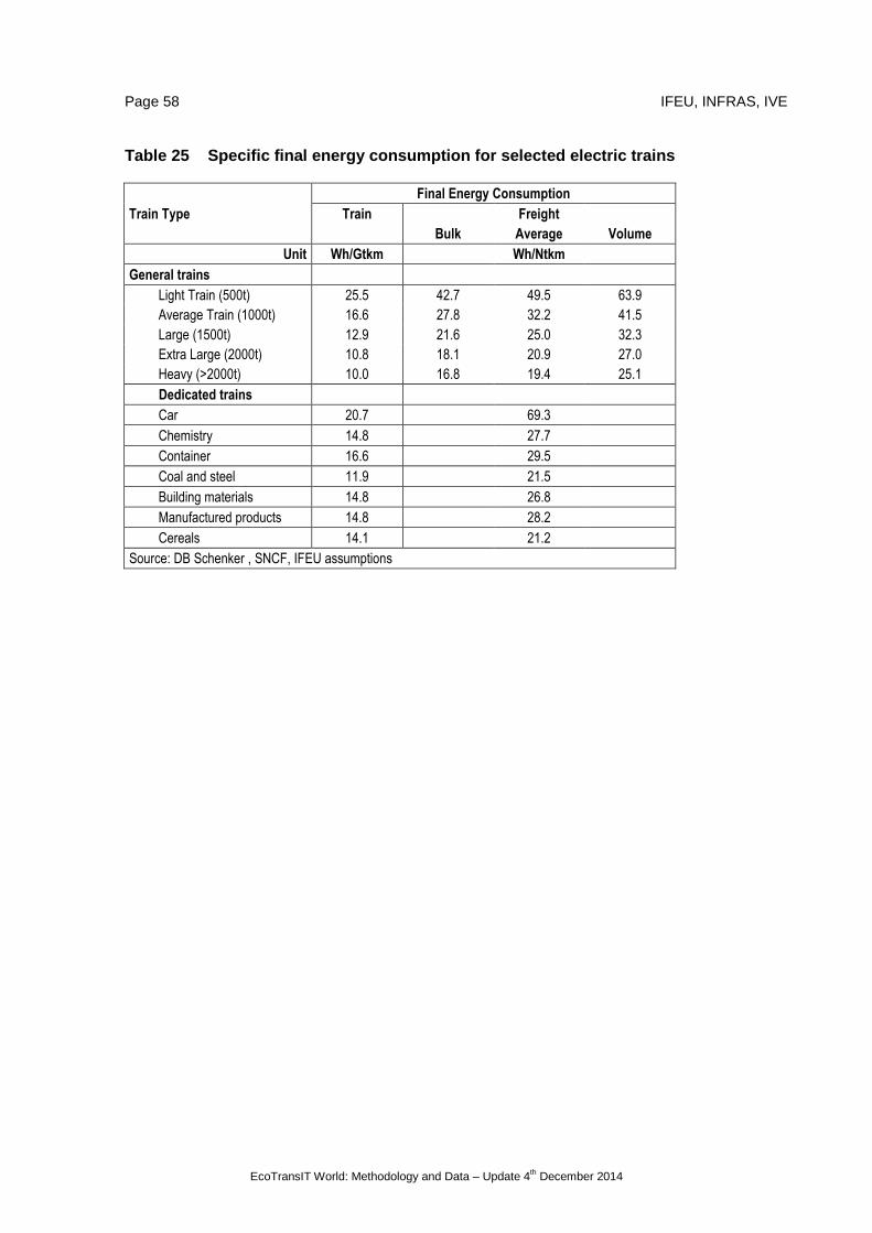
Page 58 IFEU, INFRAS, IVE
EcoTransIT World: Methodology and Data – Update 4th December 2014
Table 25 Specific final energy consumption for sele cted electric trains
Final Energy Consumption
Train Type Train Freight Bulk Average Volume
Unit Wh/Gtkm Wh/Ntkm
General trains
Light Train (500t) 25.5 42.7 49.5 63.9 Average Train (1000t) 16.6 27.8 32.2 41.5 Large (1500t) 12.9 21.6 25.0 32.3 Extra Large (2000t) 10.8 18.1 20.9 27.0 Heavy (>2000t) 10.0 16.8 19.4 25.1
Dedicated trains
Car 20.7 69.3
Chemistry 14.8 27.7
Container 16.6 29.5
Coal and steel 11.9 21.5
Building materials 14.8 26.8
Manufactured products 14.8 28.2
Cereals 14.1 21.2
Source: DB Schenker , SNCF, IFEU assumptions

IFEU, INFRAS, IVE Page 59
EcoTransIT World: Methodology and Data – Update 4th December 2014
Energy consumption of diesel trains
The available energy data for diesel traction ranges between 2.6 and 9.7 g/gross tonne km /Railways companies 2002/. New statistics show a similar range /UIC 2009/. The statistical uncertainties can be attributed to the unreliable allocation of the fuel con-sumption to different users (passenger and goods transport, shunting, etc.). Therefore, the primary energy consumption of diesel traction is estimated on the basis of the pri-mary energy consumption of electric traction. This procedure can be used, because the total efficiency of diesel traction (including the production of fuel) is similar to the total efficiency of electric traction (including electricity generation).
So the same functional dependence as that of electric traction is taken and has to be divided by the efficiency of the diesel-electric conversion for final energy consumption of 37 %. (See Chapter 5.5.6, Figure 25.).
The following table shows the resulting specific energy consumption per Gtkm and Ntkm for different diesel trains and freight types. Some available values of heavy trains from China and statistical averages for Canada and USA are added. The values of North American railways are higher than values from energy function (similar to the large train in the formula). For this reason, additional energy consumption for North American railways could be possible, but we propose to use this formula also for North America as well on account of the small North American database available.
Table 26 Specific final energy consumption for dies el trains
Final Energy Consumption
Train Type Train Freight Bulk Average Volume
Unit Wh/Gtkm Wh/Ntkm
Light Train (500t) 68.8 115.5 133.7 172.6 Average Train (1000t) 44.8 75.2 87.0 112.3 Large (1500t) 34.8 58.4 67.6 87.3 Extra Large (2000t) 29.1 48.9 56.6 73.1 Heavy (>2000t) 27.0 45.4 52.5 67.8
Values of heavy trains Average (not specified) China 2008 27
Canada 2003 33 61 US Track 1 2006 66
Source: Railion 2007, IFEU 2008, EPS 2005, USDOT 2008

Page 60 IFEU, INFRAS, IVE
EcoTransIT World: Methodology and Data – Update 4th December 2014
5.2.3 Emission factors for diesel train operation ( TTW)
Contrary to electric traction, emissions for diesel traction are also produced during the operation of the vehicle. These emission factors are stated as specific values based on the fuel consumption (in g/kg diesel fuel). Values have been made available by several European railway companies /Railway companies 2002/, the UIC Raildiesel study /UIC 2005/ and from Canada /EPS 2005/. Table 11 summarizes the emission factors for diesel trains of different railway companies. ETW uses the new values of DB 2008 for all railways.
Table 27: Emission factors for diesel trains (NOx, NMHC, PM)
Unit NOx NMHC PM
Different European Railway Companies, 2001 g/kg 40-70 1.8-5.7 0.6-5.0
UIC Rail Diesel, main locomotives (2005) g/kg 64.7 1.15
DB 2008 g/kg 48.3 4.63 (HC) 1.35
Canada 2003 g/kg 63.9 2.8 (HC) 1.4
Default ETW 2014 g/kg 48.3 4.63 1.3
kg/TJ 1,122 106 31
Source: UIC 2005, DB 2008, EPS 2005, Railway Companies 2002
Sulphur dioxide emissions depend on sulphur content on fuel. These values are coun-try-specific. The sulphur content of diesel fuel is assumed according the valid legisla-tion. In ETW, the same values for railways are used for road transport (see Chapter 5.1, Table 21).
For greenhouse gases (CO2e) the default values of EN 16258 and corresponding CO2-values are applied (see appendix, chapter 6.1)

IFEU, INFRAS, IVE Page 61
EcoTransIT World: Methodology and Data – Update 4th December 2014
5.3 Sea transport
Sea transport emission factors have been developed exclusively for ETW in contrast to those for other modes, since reliable and comprehensive literature data isn’t available. Indeed Clean Cargo Working Group publishes CO2 efficiency figures for a variety of ocean-going container ships, but it lacks emission factors for air pollutants and other maritime vessels. Therefore, it was developed an own approach for ETW based on IMO /2009/ and Buhaug /2008/ for GHG emission and air pollutant emission factors.4
The derivation of emission factors for ocean-going ships for ETW is based on a bottom-up approach. This approach for maritime vessels is based on activity and technical data and offers a reliable methodology for estimating emissions from individual ships as well as groups of ships, ship types and emissions in specific geographies. A detailed description of the ETW methodology can be found in a separate methodological paper published by ETW /Seum 2009/. The following subchapters describe only the general approach and data used for ETW. For more detailed background information the addi-tional methodological paper has to be consulted.
5.3.1 Overview of the ETW bottom-up approach
In ETW, underlying emission factors are developed for different vessel types. The ves-sel types that are differentiated are:
• General Cargo Vessels
• Dry Bulk Carriers
• Liquid Bulk Carriers
• Container Carriers
• Roll-on-Roll-off vessels (in ferry services)
Other vessels are not included in ETW because of their differing cargo specifications and lower relevance for the likely ETW user. Those vessel types include LNG and LPG gas carriers as well as car carriers. Ferries and RoRo vessels are not included in this section of the report because they are treated like extensions of the road network and are thus presented in the chapter for land transport.
The modelling of emission factors used in ETW is based on technical data of 4,616 sample vessels. The technical data was collected from Lloyds Register of Shipping /Lloyds 2009/. The validity of the sample was tested by comparing the findings with the aggregate results for CO2 emissions in the updated greenhouse gas study publishes by IMO /IMO 2009/. In general emission factors are developed for each individual vessel (EFv). The principle derivation of emission factors uses main and auxiliary engine data, capacity data and activity data. Emission factors for container vessels have been de-rived in g/TEU-km (TEU = twenty foot equivalent unit = standard container of 20’ length), whereas for all others vessels the factors are based on g/tonne-km. The EFv
4 The ETW bottom-up methodology considers also methodologies developed for marine
vessel emission inventories (e.g. /Aldrete et al. 2005/, /Anderson et al. 2003, 2004/, /CARB 2007/, /Corbett and Fischbeck 1997/, /Corbett and Köhler 2002/, /Corbett 2004/, /ENTEC 2002/, /EPA 2009/).

Page 62 IFEU, INFRAS, IVE
EcoTransIT World: Methodology and Data – Update 4th December 2014
are based first on nominal carrying capacity (100 % vessel utilisation) with the subse-quent inclusion of vessel utilisation including empty trips.
EFv = engine data x vessel capacity data x vessel a ctivity data x vessel utilisation factor
The final emission factors for the different vessel types, size classes and trade lanes are finally weighted averages of the vessels’ individual emission factors. In the extend-ed input mode of ETW, specific vessel types and size classes can be selected. In the standard mode of ETW, vessel types and size classes have been grouped to derive trade lane specific emission factors (for the definition of the trade lanes see Figure 3). The appropriate vessel emission factor is automatically chosen when selecting the type of cargo and the port pairs in the model. For example, “dry” and “liquid” bulk cargo se-lection from North America to Europe results in the calculation with an aggregate transatlantic bulk carrier. Three types of default transport loads exist within container-ized transport: volume good, average weight and heavy weight cargo. Average weight cargo is the default assumption. Bulk carriers are always calculated as carrying heavy weight cargo.
As mentioned, individual vessel emission factors are derived by calculating emissions for the main and the auxiliary engine separately and splitting the emissions into “main engine at sea”, “auxiliary engines at sea” and “auxiliary engines in port” categories. The reason for this separation is a) a differentiation of technical data, b) a differentiation of activity data and c) the desire to allow users to model speed reductions of vessels. Firstly, main and auxiliary engines have different engine load patterns at sea and in port. Secondly, depending on the vessel type and trade lane the split between at sea and in port differs. And thirdly, a vessel speed reduction only results in reduced emis-sions from main engines at sea, whereas the emissions of auxiliary engines at sea in-crease due to the longer duration of the trip and the emissions in port remain un-changed while delivering the same transport services. In order to model the effects of reduced vessel speeds, each vessel is modelled for a virtual year period in the stand-ard assumption. The emissions, both from main and auxiliary engines, are then normal-ized to one tonne or TEU kilometre, including the emissions from auxiliary engines in port. If reduced vessel speeds are modelled, the vessel’s activity extends the one year period in order to deliver the same transport services. However, emissions are again normalized to transporting one tonne or TEU kilometre /Seum 2010/.

IFEU, INFRAS, IVE Page 63
EcoTransIT World: Methodology and Data – Update 4th December 2014
Figure 16: Schematic effects of fuel consumed and g reenhouse gas emissions with slow steaming /Seum 2010/
Another split is made between fuel based and engine based emissions respectively pollutants (see chapter 3.3). Fuel based pollutants are emitted in a linear correlation to the amount of fuel burned. Engine based pollutants are emitted according to the physi-cal-chemical characteristics of the engine technology. Carbon dioxide (CO2), GHG emissions (calculated as CO2 equivalents) and sulphur oxides (SOx) are mainly fuel based emissions. Due to newly developed emission factors for nitrogen oxides (NOx), which take the new emission limits into account /IMO 2009/, NOx is also considered a fuel based emission factor, although technically it is more determined by engine tech-nologies.
Non-methane hydrocarbons (NMHC) and particulate matter (PM) are mainly engine-based emissions. NMHC and PM emission factors are calculated based on the en-gines’ power demand for transporting one tonne-km. In principle PM emissions are both fuel- and engine- based. Large parts of marine particulate emissions originate from the sulphur content in marine fuels. However, the combustion efficiency also influ-ences particulate matter emissions, in particular the soot and black carbon (BC) frac-tion. Recent studies have found not only a weak correlation between the fuel sulphur and the PM emissions, but also between engine power and PM emissions /CARB 2007/. For this study, a formula that derives PM emission factors in g/kWh, taking the fuel sulphur content into account was used /CARB 2007/.
5.3.2 Development of trade-lane specific emission f actors
The ETW model provides a standard as well as an extended input mode. Within the extended mode, emission factors for different vessel types and sizes are available and can be chosen by the user of ETW (see Table 29). For the standard input mode emis-sions have been grouped according to vessel types and sizes used for the major trade lanes. Table 28 lists all region pairs considered by ETW and defines the trade-lanes.
Tb = additional time for transportactivity Ti and slow steaming
main engine(s) at searegular speed
auxillary engine(s) at sea
auxillary Engine(s) in port
Ti Tb
main engine(s) at seaslow speed
Tb = additional time for transportactivity Ti and slow steaming
main engine(s) at searegular speed
auxillary engine(s) at sea
auxillary Engine(s) in port
Ti Tb
main engine(s) at seaslow speed

Page 64 IFEU, INFRAS, IVE
EcoTransIT World: Methodology and Data – Update 4th December 2014
Table 28: Overview of world trade lanes considered by ETW
From / To EU -
Europe NA -
North Am. LA -
Latin Am. AF -
Africa AS - Asia
OZ - Oceania
EU - Europe
Intra-con-tinental Europe
Transatlantic trade
Other global trade
Other global trade
Suez trade
Other global trade
NA - North Am.
Transatlantic trade
Intra-con-tinental (non
Europe)
Panama trade
Other global trade
Transpacific trade
Other global trade
LA - Latin Am.
Other global trade
Panama trade
Intra-con-tinental (non
Europe)
Other global trade
Other global trade
Other global trade
AF - Africa
Other global trade
Other global trade
Other global trade
Intra-con-tinental (non
Europe)
Other global trade
Other global trade
AS - Asia
Suez trade
Transpacific trade
Other global trade
Other global trade
Intra-con-tinental (non
Europe)
Other global trade
OZ - Oceania
Other global trade
Other global trade
Other global trade
Other global trade
Other global trade
Intra-con-tinental (non
Europe)
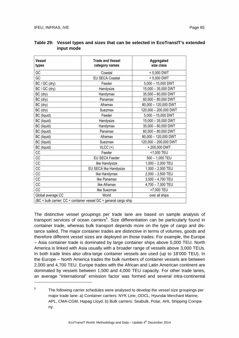
IFEU, INFRAS, IVE Page 65
EcoTransIT World: Methodology and Data – Update 4th December 2014
Table 29: Vessel types and sizes that can be select ed in EcoTransIT’s extended input mode
Vessel types
Trade and Vessel category names
Aggregated size class
GC Coastal < 5,000 DWT GC EU SECA Coastal < 5,000 DWT BC / GC (dry) Feeder 5,000 – 15,000 DWT BC / GC (dry) Handysize 15,000 – 35,000 DWT BC (dry) Handymax 35,000 – 60,000 DWT BC (dry) Panamax 60,000 – 80,000 DWT BC (dry) Aframax 80,000 – 120,000 DWT BC (dry) Suezmax 120,000 – 200,000 DWT BC (liquid) Feeder 5,000 – 15,000 DWT BC (liquid) Handysize 15,000 – 35,000 DWT BC (liquid) Handymax 35,000 – 60,000 DWT BC (liquid) Panamax 60,000 – 80,000 DWT BC (liquid) Aframax 80,000 – 120,000 DWT BC (liquid) Suezmax 120,000 – 200,000 DWT BC (liquid) VLCC (+) > 200,000 DWT CC Feeder <1,000 TEU CC EU SECA Feeder 500 – 1,000 TEU CC like Handysize 1,000 – 2,000 TEU CC EU SECA like Handysize 1,000 – 2,000 TEU CC like Handymax 2,000 – 3,500 TEU CC like Panamax 3,500 – 4,700 TEU CC like Aframax 4,700 – 7,000 TEU CC like Suezmax >7,000 TEU Global average CC World over all ships (BC = bulk carrier; CC = container vessel GC = general cargo ship
The distinctive vessel groupings per trade lane are based on sample analysis of transport services of ocean carriers5. Size differentiation can be particularly found in container trade, whereas bulk transport depends more on the type of cargo and dis-tance sailed. The major container trades are distinctive in terms of volumes, goods and therefore different vessel sizes are deployed on those trades. For example, the Europe – Asia container trade is dominated by large container ships above 5,000 TEU. North America is linked with Asia usually with a broader range of vessels above 3,000 TEUs. In both trade lines also ultra-large container vessels are used (up to 18’000 TEU). In the Europe – North America trades the bulk numbers of container vessels are between 2,000 and 4,700 TEU. Europe trades with the African and Latin American continent are dominated by vessels between 1,500 and 4,000 TEU capacity. For other trade lanes, an average “international” emission factor was formed and several intra-continental 5 The following carrier schedules were analysed to develop the vessel size groupings per
major trade lane: a) Container carriers: NYK Line, OOCL, Hyundai Merchant Marine, APL, CMA-CGM, Hapag Lloyd; b) Bulk carriers: Seabulk, Polar, AHL Shipping Compa-ny.

Page 66 IFEU, INFRAS, IVE
EcoTransIT World: Methodology and Data – Update 4th December 2014
emission factors were developed (see Table 30).
A similar approach was used for bulk vessels. However, the distinction here is based on certain size restrictions in particular regions. Some installations in the world sea infrastructure restrict the size of the vessels. The most important ones were considered in developing the vessel size classes for bulk vessels. These are the Suez Canal, the Panama Canal, and the entrance to the Baltic Sea. The Suez Canal does not pose a restriction to even the largest container ships. However, bulk carriers are limited to ap-proximately 200,000 dead weight tonnage6 (DWT). The Panama Canal poses both restrictions for bulk carriers (ca. 80,000 DWT) and container ships (ca. 4,300 TEU with some vessels up to 5,000 TEU capacity). The Baltic Sea entrance is limited to bulk vessels of maximum 120,000 DWT in general. However, the ports in the Baltic Sea are mostly served by smaller feeder vessels.7 Furthermore, the Baltic Sea as well as the North Sea are so-called Sulphur Emission Control Areas with limits on fuel sulphur at sea and in port /Sustainable Shipping 2009/. Thus a separate EU SECA trade lane was formed (see also next subchapter). The limitations are due to limits in the vessels draft, as well as length and width if locks are in place. The Panama Canal is currently under construction and will be expanded to accommodate larger vessels.
All trade-lane specific emission factors are weighted averages derived from the individ-ual sample vessels emission factors. The vessel emission factors are weighted accord-ing to the transport work of the vessels as a combination of cargo capacity and average utilisation. Table 30 shows vessel type classes depending on the trade lane for the standard mode of ETW. The standard mode doesn’t differentiate between liquid and dry bulk.
6 Dead weight tonnage (DWT) is the measurement of the vessel’s carrying capacity. The
DWT includes cargo, fuel, fresh and ballast water, passengers and crew. Different DWT values are based on different draught definitions of a ship. The most commonly used and usually chosen if nothing else is indicated is the DWT at scantling draught of a ves-sel, which represents the summer freeboard draught for seawater /MAN 2006/
7 Personal communication Port of Oslo.

IFEU, INFRAS, IVE Page 67
EcoTransIT World: Methodology and Data – Update 4th December 2014
Table 30: Default vessel categories depending on ca rgo type and trade lane
Vessel types
Trade lane
Aggregated size class
BC (liquid, dry, and General Cargo) Suez trade Aframax / Suezmax BC (liquid, dry, and General Cargo) Transatlantic trade Handymax / Panamax BC (liquid, dry, and General Cargo) Transpacific trade Handymax / Panamax / Aframax / Suezmax BC (liquid, dry, and General Cargo) Panama trade Handymax / Panamax BC (liquid, dry, and General Cargo) Other global trade Handysize / Handymax / Panamax / Aframax BC (liquid, dry, and General Cargo) Intra-continental trade Feeder / Handysize / Handymax CC Suez trade 4,700 – 7,000 (+) TEU CC Transatlantic trade 2,000 – 4,700 TEU CC Transpacific trade 1,000 – 7,000 (+) TEU CC Panama trade 2,000 – 4,700 TEU CC Other global trade 1,000 – 3,500 TEU CC Intra-continental trade non EU 500 – 2,000 TEU CC Intra-continental trade EU 500 – 2,000 TEU Great Lake BC < 30,000 DWT
Note: BC = bulk carrier, GC = general cargo ship, CC = container vessel
5.3.2.1 Sources of basic emission factors for marin e vessels (Tank-to-Wheels)
Main engines
In a first step the final energy consumption (TTW) of the marine vessels is calculated considering the engine power and engine load of the different ocean-going vessels considered within ETW. This approach is described in detail in /Seum 2010/. Modelling fuel consumption requires additional assumptions, such as days at sea (for modelling the reduced speed option), the nominal design speed (Vn) and the percentage of heavy fuel oil (HFO). Table 31 lists the main assumptions used for calculating the fuel consumptions and emissions of ocean-going vessels. Those assumptions are averag-es for the respective vessels for particular trade lanes as defined in Table 30 and for individual vessel classes that can be selected in the extended input mode of ETW.

Page 68 IFEU, INFRAS, IVE
EcoTransIT World: Methodology and Data – Update 4th December 2014
Table 31: Days at sea, design speed (Vn), share of heavy fuel oil and default vessel utilisation factors that are used in ETW.
The design speed for container vessels used in this table still shows speed levels which are no longer real. Technical adjustments have been made to reduce design speed, resulting in even lower service speed.
For the default standard mode all vessels were modelled assuming an average speed reduction of 25% below the nominal design speed8. The vessel speed may be altered in the extended input mode. Slow steaming is one measure of temporarily lowering
8 The average speed reduction is based on analyses of the internet page
http://www.searates.com. In the ETW report from 2010 a speed reduction of only 4% was used. Due to enlargement of slow steaming currently the speed reduction is much higher.
Vessel type Trade Size class Days at sea Vn km/h%
HFO
BC (liquid, dry, and General Cargo) Suez trade Aframax / Suezmax 259 27.2 100%BC (liquid, dry, and General Cargo) Transatlantic trade Handymax / Panamax 250 26.8 99%BC (liquid, dry, and General Cargo) Transpacific trade Handymax / Panamax / Aframax / Suezmax 253 27.0 100%BC (liquid, dry, and General Cargo) Panama trade Handymax / Panamax 250 27.0 99%BC (liquid, dry, and General Cargo) Other global trade Handysize / Handymax / Panamax / Aframax 250 27.0 99%BC (liquid, dry, and General Cargo) Intra-continental trade Feeder / Handysize / Handymax 242 26.6 98%CC Suez trade 4700 - 7000 (+) TEU 246 46.3 100%CC Transatlantic trade 2000 - 4700 TEU 251 41.6 100%CC Transpacific trade 1000 - 7000 (+) TEU 253 40.3 100%CC Panama trade 2000 - 4700 TEU 251 41.6 100%CC Other global trade 1000 - 4700 TEU 255 38.7 100%CC Intra-continental trade non EU 1000 - 3500 TEU 256 37.5 100%CC Intra-continental trade EU 500 - 2000 TEU 228 34.1 100%CC EU SECA trade 500 - 2000 TEU 228 34.1 80%Great Lakes BC < 30000 dwt 238 26.3 96%Ferry / RoRo vessel World Large > 2000 lm 219 36.9 33%Ferry / RoRo vessel World Small < 2000 lm 180 37.4 55%Ferry / RoRo vessel EU SECA Large > 2000 lm 219 36.9 16%Ferry / RoRo vessel EU SECA Small < 2000 lm 180 37.4 30%GC Coastal < 5000 dwt 180 25.4 100%GC EU SECA Coastal < 5000 dwt 180 25.4 70%BC / GC (dry) Feeder 5000 - 15000 dwt 244 26.4 99%BC / GC (dry) Handysize 15000 - 35000 dwt 256 27.6 99%BC (dry) Handymax 35000 - 60000 dwt 261 26.6 99%BC (dry) Panamax 60000 - 80000 dwt 270 26.4 99%BC (dry) Aframax 80000 - 120000 dwt 271 26.0 100%BC (dry) Suezmax 120000 - 200000 dwt 279 26.9 100%BC (liquid) Feeder 5000 - 15000 dwt 203 23.2 79%BC (liquid) Handysize 15000 - 35000 dwt 228 26.8 100%BC (liquid) Handymax 35000 - 60000 dwt 231 27.1 100%BC (liquid) Panamax 60000 - 80000 dwt 196 27.3 100%BC (liquid) Aframax 80000 - 120000 dwt 247 27.1 100%BC (liquid) Suezmax 120000 - 200000 dwt 270 27.8 100%BC (liquid) VLCC (+) > 200000 dwt 274 27.8 100%CC Feeder <1000 TEU 180 31.7 100%CC EU SECA Feeder 500 - 1000 TEU 180 31.7 80%CC like Handysize 1000 - 2000 TEU 259 35.5 100%CC EU SECA like Handysize 1000 - 2000 TEU 259 35.5 80%CC like Handymax 2000 - 3500 TEU 251 40.1 100%CC like Panamax 3500 - 4700 TEU 250 44.7 100%CC like Aframax 4700 - 7000 TEU 248 46.2 100%CC like Suezmax >7000 TEU 242 46.7 100%Global average CC World over all ships 238 38.6 100%Source: Buhaug 2008, own calculation

IFEU, INFRAS, IVE Page 69
EcoTransIT World: Methodology and Data – Update 4th December 2014
emissions9. The emission reduction effect is due to an over-proportional decline of the emissions compared to the service speed. Thus, while the vessel carrying capacity in a given time period diminishes, the emissions diminish even more, resulting in a net-reduction of emissions per tonne-kilometre. ETW allows users to model seaborne emissions down speed reductions up to 30 % of the speed based on the vessel’s de-sign speed. The positive benefit of speed reductions below 30 % disappears and en-during operation of marine engines at very low engine loads is not recommended by engine manufacturer without modifications to the engines.
Based on the TTW energy consumption fuel based emissions are calculated in a sec-ond step. As mentioned in chapter 5.3.1 CO2, CO2 equivalents, SOx and NOx are di-rectly linked to the fuel consumption. For ETW CO2 emission factors are used based on the same sources than the CO2 equivalent emission factors of the European standard EN 16258 (original data source is IMO, see Table 52 in the annex). The values applied for ETW are included in Table 32. For CO2 equivalent the emission factors included in the EN 16258 are used without changes (see Table 51 in the annex).
Table 32: Marine fuels, main engine emission factor s and sources for CO 2 and nitrogen oxide emissions
For emissions of CO2 / CO2 eq & NOx Source: Emission factors
[g/kg fuel]
CO2 / HFO based on EN 16258 3,11 CO2 / MDO&MGO based on EN 16258 3,21 NOx SSD pre Tier I IMO 2009 89.5 NOx SSD Tier I IMO 2009 78.2 NOx MSD pre Tier I IMO 2009 59.6
NOx MSD Tier I IMO 2009 51.4
Sources: IMO 2009; EN 16258. Note: SSD = slow speed diesel engines; MSD = medium speed diesel engines.
NOx emissions are mainly engine related. Until the year 2000, marine engines were unregulated. In 1997, revisions to the Annex VI of the International Convention on the Prevention of Pollution from Ships Tier I standards for marine engines were adopted, that became effective in January 2000. The standard manifested the status quo at that time and was tightened further in 2008 by adopting Tier II and Tier III standards. Tier II emission standards are effective for any new engine or major overhaul from 2011 and will also be able to adhere to by adjusting common diesel engines to those standards. The Tier II NOx adjustment may come with a slight fuel penalty /MAN 2006/, because leaner burning processes for lower NOx means less optimal combustion processes with higher fuel consumption and higher particulate matter emissions. Tier III standards which will come into effect for Emission Control Areas in 2016 may only be achieved through the application of additional exhaust gas cleaning. For NOx emission the emis-sion factors by IMO /2009/ were used, which differentiate between pre Tier I and Tier I (pre 2000 and after) as well as between slow speed and medium speed diesel engines. The factors reflect the IMO’s NOx code formula /MEPC 2008/. However, because the
9 A permanent related measure would be the downsizing or de-rating of the main engine.

Page 70 IFEU, INFRAS, IVE
EcoTransIT World: Methodology and Data – Update 4th December 2014
exact engine returns per minute were not known, the IMO /2009/ were applied (see Table 32).
Sulphur oxide emissions are calculated based on the sulphur content in marine fuels. The mass of sulphur in marine fuels is expressed in mass percentage. It is assumed that 97.7 % of the fuel sulphur in fuels is oxidised during combustion /EPA 2009/. The corresponding sulphur oxide emissions are derived by multiplying the mass with the factor of two. For each region, different sulphur levels in fuel apply. Generally the global average sulphur level is assumed to be 2.37 % in heavy fuel oil /MEPC 2009b/. For auxiliary engines, lower sulphur levels were assumed because of the partial use of ma-rine diesel oil (MDO) and marine gas oil (MGO) for those engines. Furthermore, for the in-port and Sulphur Emission Control Areas (SECA; see also chapter 5.3.2.2) different sulphur levels were assumed. The sulphur contents used for ETW are documented in Table 33).
Table 33: Sulphur content of fuels used for ocean-g oing vessels depending on sea regions and engine types
Sea region Engine-type S general
[%]
S in SECA
[%]
General open sea and in port Main engine HFO 2.37 1.0
General open sea and in port Main engine MDO/MGO 1.5 1.0
General open sea Auxiliary engine 1.5 1.0
In port Auxiliary engine 0.5 0.1
Sources: MEPC 2009b; AKN 2009.
Particulate matter emissions are important for local air quality. However, to date uncer-tainties of the extent of particulate matter emissions and emission factors are quite large. Particles from marine engines are depending on the efficiency of the combustion process and also on the amount of sulphur in marine fuels. Approximately 10 % of the fuel sulphur is oxidised to Sulphates (SO4), which directly contributes to the fine parti-cles in the exhaust and dominates the particulate matter emissions /Janhäll 2007/. However, a recent compilation of research has found only weak correlations between the fuel sulphur levels and the particulate matter emissions of ships /CARB 2007/. The findings further reflect the difficulties to measure particulate matter emissions and the limited number of empirical data. In order to derive the emission factors the formula developed by CARB /2007/ was used. Table 34 provides the emission factor at the fuel sulphur levels used in ETW depending.
Table 34: Particulate matter emission factors for m ain and auxiliary engines
S-content
2.70% [g/kWh]
S-content 2.37%
[g/kWh]
S-content 1.50%
[g/kWh]
S-content 1.00%
[g/kWh]
S-content 0.50%
[g/kWh]
S-content 0.10%
[g/kWh]
PM 10 1.51 1.35 0.95 0.72 0.48 0.30 PM 2.5 (90% of PM10) 1.36 1.22 0.85 0.64 0.43 0.27
Sources: CARB 2007, Janhäll 2007.

IFEU, INFRAS, IVE Page 71
EcoTransIT World: Methodology and Data – Update 4th December 2014
Main engine emission factors for non-methane hydrocarbons were taken from EPA /2009/. With its guidance on developing emission inventories of port areas, EPA has compiled a comprehensive list of factors and published valuable average emission and activity figures for main and auxiliary engines. The emission figures for main engines are differentiated for slow speed marine diesel (SSD) engines using heavy fuel oil (HFO), medium speed marine diesel (MSD) engine using marine diesel oil (MDO) and steam turbines (ST). The emission factors for the SSD and MSD engines were used in ETW. Steam turbine powered vessels are ignored because of their small number (Table 35).
Table 35: NMHC emission factors of the main engine
SSD using HFO
[g/kWh] MSD/SSD using MDO/MGO
[g/kWh]
NMHC 0.60 0.50 Note: SSD = slow speed diesel; MSD = medium speed diesel; HFO = heavy fuel oil; MDO = marine diesel oil; MGO = marine gas oil Source: EPA 2009.
Auxiliary engines
For auxiliary engines the assumptions were also taken from Buhaug et al. /2008/ and EPA /2009/. Depending on the auxiliary engine power, a fuel consumption of either 230 g/kWh for engines with less than 800 kW or 220 g/kWh for engines with 800 kW and more was used /Buhaug et al. 2008/. For the emissions at sea, it was assumed that the auxiliary engines are fuelled with the same type of marine fuels as the main en-gines. In port it is assumed that auxiliary engines are fuelled with low-S marine diesel oils of 1.5 % generally and 0.1 % S in European ports due to EU regulations. Thus sul-phur oxide emissions were calculated accordingly. For NOx and HC emission factors were taken from EPA /2009/. CO2 equivalent emission factors are based on EN 16258.
Table 36: NOx, NMHC, PM and SO 2 emission factors for auxiliary engines
Pollutants MSD HFO
2,7% S [g/kWh]
MSD MDO 1,0% S [g/kWh]
MSD MGO 0,5% S [g/kWh]
MSD MGO 0.,1% S [g/kWh]
NOx 14.7 13.9 13.9 13.9 NMHC 0.40 0.40 0.40 0.40 PM Like main engine
SO2 11.98 4.24 2.12 0.42
Sources: EPA 2009; Janhäll 2007.
5.3.2.2 Emissions in Sulphur Emission Control Areas
Dedicated emission factor were developed for trade lanes within the sulphur emission control areas (SECA) in the North and Baltic Sea (see Figure 17). If in ETW a user sets the start and end point within the boundaries of the SECA, the emission factors for sul-

Page 72 IFEU, INFRAS, IVE
EcoTransIT World: Methodology and Data – Update 4th December 2014
phur oxides and particulate matter are reduced automatically due to the use of low-sulphur fuels. Furthermore, specific vessels may be picked in the expert extended input mode.
The vessels that are travelling in the SECA areas are assumed to operate more often on marine diesel oils. Several ports in the Baltic Sea region have instituted emission differentiated harbour dues, recommended by the Helsinki Convention /HELCOM 2007/. Thus, in traffic to those ports, additional incentives exist to reduce NOx emis-sions as well as SOx emissions. The technologies used to achieve lower NOx emis-sions are Selective Catalytic Reduction (SCR) and Direct Water Injection (DWI). SCR technology requires low-sulphur fuels and thus can best operate with MDO or MGO. Thus, the share of HFO oil as fuel is reduced to 70 % for general cargo vessels and 80 % for container vessels, assuming that more general cargo vessels are on dedicat-ed trades within the SECA region. Other emission factors that would reflect the use of advanced after treatment were not considered for ETW.
Figure 17: Demarcation of the North and Baltic Sea SECA /Sustainable Shipping 2009/
5.3.3 Allocation rules for seaborne transport
The emissions of ocean-going vessels are averaged over the entire return journeys, taking the load factors and empty returns into account. Furthermore, emissions are the sum of emissions from main engines at sea, auxiliary engines at sea and auxiliary en-

IFEU, INFRAS, IVE Page 73
EcoTransIT World: Methodology and Data – Update 4th December 2014
gines in port. All emissions are then allocated to the freight carried.
For bulk vessels the allocation unit is tonne-kilometre. All emissions are allocated to the product of transported tonnes of freight and distance travelled. The emissions of con-tainer vessels are calculated on a container-kilometre basis (TEU-km). All emissions are allocated to the number of containers and distance. If the user knows the weight and type of its cargo, but not the number of containers, the weight is converted into the number of containers firstly by using the container weights presented in Table 9 for volume, average and bulk goods. If the user chooses TEU as type of freight and knows the number of containers transported than the net-weight of the containers matters only for the on- and off-carriages.
5.3.4 Allocation method and energy consumption for ferries
The modelling of ferries is tricky because all vessels are quite different from each other and the allocation between passenger and goods transport is a controversial issue. So different allocation methodologies are proposed, e.g. by /Kristensen 2000/ or /Kusche 2000/.
For ETW we use the allocation method which has been suggested for the calculation model of NTM by /Bäckström 2003/. This method allocates according to the number of decks on the ferry. The number of passenger and vehicle decks is considered in the first step of the allocation. It should also be taken into account if these decks are only partially used for certain vehicle categories or if they do not extend over the full length of the ship. The second step of the allocation divides the length of lanes (lane metres) occupied by the considered vehicles by the total length of the occupied lanes.
The following fuel related average values have been calculated according to this meth-od for a concrete example of TT-Lines. It replaces the values of Scandlines ferry, which were used until 2008-:
Lorry (30 gross tonnes) 18 g fuel/gross-ton-km
Railcar (46 gross tonnes) 18 g fuel/gross-ton-km
These values are taken and differentiated according to vehicle types and kind of good. The resulting specific energy values are summarised in the following table.
Table 37 Specific Energy Consumption for ferries
Final energy consumption (g fuel/Ntkm)
Rail Truck <7.5t Truck 7.5-12t Truck 12-24t Truck 24-40t
Bulk (heavy) 31 52 48 38 34 Average 36 60 55 43 38
Volume (light) 46 95 86 63 55
Source: Bäckström 2003, TT Lines 2009, IFEU assumptions
These values represent a ferry example and are derived by a concrete allocation method. They indicate the order of magnitude, but may vary a lot for other ferries and ferry companies.

Page 74 IFEU, INFRAS, IVE
EcoTransIT World: Methodology and Data – Update 4th December 2014
5.4 Inland waterway transport
5.4.1 General approach and assumptions for inland v essels
Inland vessels are approached similarly to ocean going vessels. A bottom-up modelling based on assumptions for each vessel classes was used.
ETW faces the challenge to cover the entire world. There are only few waterways worldwide that are considered in ETW. The majority of waterways are in Europe. Most prominent are the rivers Danube, Elbe, Rhine, and Seine10, which are (at least in sec-tions) categorised as class VI according to the UNECE code for inland waterways /UNECE 1996/. Other rivers and canals in Europe are of class V or smaller. Figure 18 depicts the European waterways. All European waterways class IV and higher are in-cluded in ETW.
Figure 18: European inland waterways and their clas sification
Prominent non-European waterways are the Mississippi in the United States. World-wide approximately 50 countries have navigable waterways of more than 1000 km length. However, inland freight navigation is underdeveloped in most countries /BVB 2009/. ETW enables inland waterways calculation on the largest of the global water-ways, such as the Yangtze, Ganges and Amazonas.
10 There are other smaller sections that are technically “inland waterways” but are treated
as part of the ocean network in EcoTransIT World. Those include the Weser up to Bremerhaven or the North-Baltic-Channel.

IFEU, INFRAS, IVE Page 75
EcoTransIT World: Methodology and Data – Update 4th December 2014
Figure 19: Worldwide inland waterways and harbours in ETW.
The distinction between inland waterways up to class IV and those of classes V and VI is important, because the size and carrying capacity of the inland barges significantly increases on class V and larger rivers. The maximum vessel size on a class IV river is an Europa ship, whereas class V and higher waterways may be travelled by larger push boats and vessels of the JOWI class. ETW differentiates between two inland barges and allocates them to particular inland waterways.
Figure 20: Inland vessel configuration as motor shi p (Europaship-type), motor ship with barge and push boat with four barges. Sou rce: Günthner et al. 2001.
The used vessels and their characteristics are presented in Table 38. Typical vessels were used in order to model the emissions. It was further assumed that the vessels are equipped with Caterpillar (Cat) engines, which are representative, to provide some

Page 76 IFEU, INFRAS, IVE
EcoTransIT World: Methodology and Data – Update 4th December 2014
technical data. Fuel consumption was taken from engine specifications by Caterpillar and a tolerance of 5 % was added.
Table 38: Typical characteristics of inland vessels
Vessel type Cargo capacity [t]
TEU capacity
ME power [kW]
Aux power [kW]
Engine example
Fuel con-sumption g/kWh11
IV, Neo K 655 N/A 336 102 1x Cat 3408C 229
IV, Europa ship 1 350 (100) 650 260 1x Cat 3508B 223
Va, RoRo, Container 2 500 200 1 140 456 1x Cat 3512 211
Va, Tank ship 3 000 N/A 1 460 585 1x Cat 3516 212
VIa, JOWI ship 5 500 470 - 500 3 200 1 000 2x Cat 3516 212
VIb, Push Convoy (4 units)
7–16 000 (11 000)
1 100 4 000 1 200 3x Cat 3516 209
The two river categories (<IV and >IV) are used in ETW and two distinct aggregate averages are built. The aggregate emission factors were built by weighing the different vessel sizes and combining them to a vessel class IV (Europaship and Neo K) and vessel >IVa. It is assumed that on rivers of category V and up both Europaship vessels and larger vessels can be found. Thus the category >IV includes the Europaship-type vessels. Vessels smaller than Neo K vessels are not considered in ETW because of their minor role in freight transport.
ETW does not take the direction of travel into account in order to treat all modes of transport similarly12. The principle of ETW is that the differences on transport legs are averaged over the entire leg because it is assumed that the transport purchaser cannot be made responsible for different performances in particular directions but has to bear responsibility for the average performance overall. For example, differences in capacity utilisation are averaged over the entire return leg. Similarly the fuel consumed per dis-tance travelled in flowing rivers, such as the Rhine, is averaged. Different fuel con-sumptions per distance up- and down-river are respectively not considered. A transport purchaser takes responsibility of the average performance regardless of the direction of the transport.
5.4.2 Emission factors for inland vessels (TTW)
Marine engines installed before 2002 in Europe and 2004-07 in North America are so called Tier 1 engines. Today, due to the average age of inland vessels, the emission Tier 2 standards play practically no role. In the Planco study /2007/, emission factors were averaged over vessel classes depending on their age profile using a regression analysis form the Tier 2 regulations. However, the resulting emission factors were not significantly above the Tier 2 limits; even for those vessels in class categories of old
11 Including a +5 % tolerance.
12 Ocean going vessels and aircrafts also have different fuel consumptions over ground depending on ocean currents and winds.

IFEU, INFRAS, IVE Page 77
EcoTransIT World: Methodology and Data – Update 4th December 2014
age. Emission factors for Category 1 engines prior to regulation were used for emis-sions inventory of inland water traffic in the Great Lakes region /Lindhjem 2004/. Since off-road diesel engines in North America and Europe are essentially the same13, those emission factors were used for ETW. The factors differentiate between engines with less than 1000 kW and those with 1000 kW and more. Most engines on inland vessels are between 500 and 2000 kW and fall in the emission threshold category 1 with 2.5 to 5 litre displacement.
Sulphur dioxide emissions depend on the fuel sulphur levels. In Europe those are re-stricted to 1000 ppm14 or 0.1 % for domestic marine diesel fuels. In the United States, non-road diesel fuel’s sulphur levels were reduced to 500 ppm in 2007 and will be fur-ther reduced to 15 ppm starting in 2010. Fuel consumption is estimated between 200 g/kWh /Planco 2007/ and 210 g/kWh (Lindhjem 2004). Our own research based on manufacturer data by Caterpillar and Cummins indicate that fuel consumption is ap-proximately 210 g/kWh for engines >1000 kW and 220 g/kWh for engines < 1000 kW /Caterpillar 2006/.
Push boats and tug boats are the dominant inland vessels in North America /Lindhjem 2004/, except for deep draft vessels that provide the link service between Great Lakes destinations and the deep sea port in Montreal. Vessels in US domestic traffic are listed in a data base by the US Army Corps of Engineers /USACE 2009/. An analysis revealed that 90 % of the push boats have less than 3200 kW. 50 % of the push boats have less than 760 kW. Thus, the US inland vessels are principally of the same size as their counterparts in Europe. The only difference is lower fuel sulphur contents of 15 ppm or 0.0015 %.
Table 39: Basic emission factors for inland vessels used for ETW /Source Lindhjem 2004/
CO [g/kWh] HC [g/kWh] NOx [g/kWh] SOx [g/kWh] PM [g/kWh]
< 1 000 kW 1.5 0.27 10.0 0.6 – 4 0.3
> 1 000 kW 2.5 0.27 12.99 0.6 – 4 0.3
Analogue to modelling the ocean going vessels, the emission factors were calculated on the basis of individual vessels, assuming the transport work for one theoretical year. In order to build the weighted averages per aggregate class, the number of inland ves-sels of particular size /Planco 2007, Table 40/ was allocated to the modelling vessels. For push boats, it was assumed that a push boat with a certain power pushes a certain number of barges and thus determines in relation to its power the total transport work of the category push boat (Table 40). The combined capacity utilisation (cargo load factor when laden and empty return trips) of bulk inland vessels is assumed to be 45 % with smaller vessels and 60 % with larger vessels (Table 40). Container carrying inland vessels are assumed to reach a capacity utilisation of 70 %.
13 The off-road engine manufacturer and the off-road engine market is a global market
with few large players providing the bulk of the commercially available global marine off-road engines, including Wärtsila (Sulzer), MAN-BW, Caterpillar and Cummins.
14 ppm = parts per million

Page 78 IFEU, INFRAS, IVE
EcoTransIT World: Methodology and Data – Update 4th December 2014
The theoretical carrying capacity of all German inland vessels is three times the real transported amount of cargo. Thus, it was assumed that vessels are only utilised 1/3 of the year. The remainder of time they lay idle with only auxiliary engines running for half the time and receiving onshore power the other time. It was further assumed that on the empty voyages vessels would require 40 % less power due to a larger freeboard and distance to the bottom of the rivers and channels /general reference on the effect see Planco 2007/. All emissions from full and empty voyages as well as during time in port are normalised to the transport of one tkm.
Table 40: Assumption of vessel number, vessel utili sation and overall transport work per year for bulk inland vessels
Ship Type Subtype Cargo utilisation Number per class Transport work per year [tkm]
Class IV Neo K 0.45 230 2 080 000 000 Class IV Europaship 0.45 670 12 699 000 000 Class Va RoRo 0.60 186 9 430 000 000 Class Va Tankship 0.45 128 5 841 000 000 Class Via JOWI Schiff 0.45 12 1 545 000 000 Class Vib Push Convoy 0.60 111 29 675 000 000 For number and transport work: Planco 2007
The resulting emission factors with average weight cargo for container transport are presented in Table 41. The lower emission factors for container carrying inland vessels compared to the bulk carrying inland vessels are a result of the better vessel utilisation rates.
Table 41: Emission factors for inland vessels, Cont ainer transport figures rep-resent the average container load of 10.5 t/TEU
5.4.3 Allocation rules for inland vessels
For inland vessels the same allocation rules than for ocean going vessels apply (see chapter 5.3.3).
Ship Type Standard typeDead weight
tons
CO2 SUM
[g/t-km]
CO2 eq SUM
[g/t-km]
Nox SUM
[g/t-km]
SOx SUM
[g/t-km]
HC SUM
[g/t-km]
PM10 SUM
[g/t-km]
Inland Barge all others EURO ship like <2000 t 60.64 61.23 0.88 0.38 0.0237 0.0260 Inland Barge Rhine, Mississipi waterway > Klasse V) > class Va >2000 t 37.74 38.11 0.65 0.24 0.0152 0.0167 Inland Barge Container all others EURO ship like <2000 t 52.69 53.20 0.76 0.33 0.0206 0.0226 Inland Barge Container Rhine, Mississipi waterway > Klasse V) > class Va >2000 t 31.50 31.80 0.54 0.20 0.0127 0.0139

IFEU, INFRAS, IVE Page 79
EcoTransIT World: Methodology and Data – Update 4th December 2014
5.5 Air transport
5.5.1 Type of airplanes and load factor
The type and model of airplanes (e.g. Boeing 747-400, B777F) used for air cargo has a high impact on GHG emissions and air pollutants. On the one hand the type gives the information about the capacity of the airplane and age of the turbine used. On the other hand the aircraft type delivers information if air cargo is transported in dedicated freighters (only for freight) or together with passengers in aircrafts (so-called belly freight). This information is important for the allocation methodology (see subchapter 5.5.4). Table 42 shows an overview of all types of aircrafts which are available within the extended input mode of ETW.
Table 42 Type of dedicated freighter and passenger aircrafts considered
Dedicated freighters Passenger aircraft
Airbus 300-600F Airbus 319
Airbus 310-300F Airbus 320
Airbus 330-200F Airbus 321
ATR 72-200F Airbus 330-200
BAe 146-300QT Airbus 330-300
Boeing (McDonnell Douglas) MD-11F Airbus 340-600
Boeing 727F Airbus 380-800
Boeing 737-300SF Boeing (McDonnell Douglas) MD-90
Boeing 747-200F Boeing 737-400
Boeing 747-400F Boeing 737-800
Boeing 747-8F Boeing 747-400
Boeing 757-200PF Boeing 747-8i
Boeing 767-200F Boeing 757-200
Boeing 777-200F Boeing 767-300
Boeing 777-200/200ER
Boeing 777-300ER
Boeing 787-8
Embraer 190
Sources: www.airbus.com; www.boeing.com; Lang 2007 und 2009; INFRAS.
Each aircraft is characterised by both: a maximum possible design range and a max-imum payload (maximum freight weight). Large passenger aircrafts can fly without stopovers more than 10,000 km, whereas smaller ones have maximum ranges of 2,000 to 3,000 km /Lang 2009/. Aside from that, larger aircrafts can transport more freight than smaller ones. The maximum payload capacity of larger aircrafts is much higher. ETW includes a wide range of small, medium and large aircrafts covering the whole possible spectrum of operating distances and payloads, which is shown exem-plarily for freighter in Figure 21. ETW considers only the so-called design range of the aircrafts, which is the maximum range for the case if the whole structural payload is utilised /Hünecke 2008/. Beyond this range the payload has to be reduced due to the additional fuel needed for the longer flight. This possibility is not considered by ETW.

Page 80 IFEU, INFRAS, IVE
EcoTransIT World: Methodology and Data – Update 4th December 2014
Figure 21 Design ranges and maximum payload capacit ies of selected dedicat-ed air freighters
Within the extended input mode ETW provides only aircrafts suitable for the flight distance between the selected airport pair. If the trip distance is longer only those aircrafts are offered by ETW that are able to fly this distance. The longer the flight, the fewer the types of aircrafts provided (see Figure 21). Additionally the aircrafts are distinguished between dedicated freighter and passenger aircrafts. The characteris-tics of all freighter and passenger aircrafts included in EcoTransIT are available in Table 54 in the annex. In the extended input mode of ETW, all aircraft types are available and may be chosen by the user.
In the standard input mode of ETW, an own selection of airplanes is not possible. Rather, ETW use the airplanes of Table 42 depending on the flight distance (up to 1,000 km short haul aircrafts; over 1,000 km up to 3,700 km medium haul aircrafts; more than 3,700 km long haul aircrafts). Because the user of the standard input mode generally don’t know whether a dedicated freighter or passenger aircraft is used ETW uses a mix of both aircraft types. This mixed aircraft type is called “hybrid aircraft”. Worldwide around 60% of air cargo is transported by freighter /e.g. IATA 2013; Airbus 2013/. This share is used for the hybrid aircrafts of EcoTransIT independent of flight distance. Thus, if a user of the standard input mode selects airports EcoTransIT cal-culates firstly the distance of the flight (e.g. 5,200 km). In the next step EcoTransIT identifies the freighter and the passenger aircrafts fitting to the flight distance (in this case Boeing 747-400F and Boeing 747-400). In the last step energy consumption and emissions are calculated for both aircraft types and mixed by the share 60% freighter and 40% belly freight. In the standard mode EcoTransIT shows only the mixed result of this hybrid aircraft.
0
20
40
60
80
100
120
140
160
0 1,000 2,000 3,000 4,000 5,000 6,000 7,000 8,000 9,000
Max
. pa
yloa
d ca
paci
ty in
tonn
es
Design range in km
Boeing 727F
BAe 146-300QT
Boeing 737-300SFATR 72-200F
Airbus A300-600F
Airbus A310-300FBoeing 767-200F
Boeing 757-200PF
Boeing 747-200F
Boeing (McDonnell Douglas) MD-11F
Airbus A330-200F
Boeing 747-8F
Boeing 747-400F
Boeing 777-200F

IFEU, INFRAS, IVE Page 81
EcoTransIT World: Methodology and Data – Update 4th December 2014
Table 43 Characteristics of selected aircrafts
Type Distance Group
Type of aircraft
IATA Aircraft
code
Design Range (km)
Max. Pay-load (t)
Typical Seats
(number)
Freighter Short haul Boeing 737-300SF 73Y 3,030 19.7
Freighter Medium Haul Boeing 767-200F 76X 5,790 45.0
Freighter Long haul Boeing 747-400F 74Y 8,250 113.0
Belly Freight Short haul Embraer 190 E90 3,330 1.4 98
Belly Freight Medium Haul Airbus 320 320 5,700 2.4 150
Belly Freight Long haul Boeing 747-400 744 13,450 16.8 416
Sources: Lang 2007; Lang 2009; LCAG 2014.
Mainly high value volume or perishable goods are shipped by air freight and the per-missible maximum weight is limited. Therefore only the category volume goods are included within the ETW tool – independent of using standard or extended input mode. Other types of goods (bulk, average) are not available for air cargo. The load factors used for volume goods differentiated by short, medium and long haul are con-tained in chapter 3.2.3.
5.5.2 Energy consumption and emission factors (Tank -to-Wheels)
Specific TTW energy consumption and TTW emissions of air cargo transportation depend heavily on the length of the flight. This is caused by different energy needs and emissions in different phases of flight (e.g. take-off or climb). Due to the data sources used by ETW this dependency from flight distance is considered for air pollu-tants like NOx, NMHC and PM. For fuel consumption the data source used (EUROCONTROL “Small Emitters Tool”, see below) only considers a linear correla-tion between energy consumption and flight distance. This simplification is legitimate since most air cargo flights are long haul flights where take-off and landing phases don’t dominate the overall energy consumption of the whole flight. Furthermore, ener-gy consumption and emissions depend on utilisation of the capacity of aircrafts (utili-sation of payload capacity). Whereas this dependency is considered by road transport, this was not able for aircrafts due to lack of available data. But the possible error is small and therefore justifiable.
The basis of fuel consumption for the different airplanes considered by ETW is the EUROCONTROL “Small Emitters Tool”15 which has been developed on behalf of the European Commission for reporting under the European Emissions Trading Scheme (ETS) /EUROCONTROL 2009 and 2013a/. This data source is updated on a regular basis and covers a wide range of aircrafts and aircraft families including many newer ones /DECC 2014/. The Small Emitters Tool covers more than 400 different aircraft types including turboprop engines. EUROCONTROL gathers, on a regular basis and from volunteer aircraft operators in Europe, samples of actual fuel-burn data for their flights performed in a specific year (e.g. 2013). Based on this fuel-burn data a linear regression is carried out for each aircraft type in the sample to consider the fuel de-
15 See also http://www.eurocontrol.int/articles/small-emitters-tool.

Page 82 IFEU, INFRAS, IVE
EcoTransIT World: Methodology and Data – Update 4th December 2014
pendency from distance flown (see for example in Figure 22) /EUROCONTROL 2009/. In total measured energy consumptions are available for around 70 different aircraft types in the Small Emitters Tool.
In a second step the Small Emitters Tool uses conclusions by analogy for aircraft families. That means that for aircrafts without measured fuel-burn data the energy consumption of other aircraft types of the same family are used (e.g. fuel-burn data from B747-400 for B747-300). In these cases the measured data are adjusted by us-ing a correction factor based on the MTOW (maximum take-off weight) ratio /EUROCONTROL 2009/. This approach is used for around 30 airplanes. In a third step data from the EMEP/EEA Air Pollutant Emission Inventory Guidebook (formerly called the EMEP CORINAIR Emission Inventory Guidebook) is used for around 30 airplanes /EEA 2013/. Last but not least for the remaining aircraft types (around 270) the average fuel consumption per flight kilometre is calculated based on linear re-gression model based on the available data considering the MTOW of each airplane /EUROCONTROL 2009/.
Figure 22 TTW energy consumption of the Small Emitt ers Tool is based on a linear regression of fuel-burn data collected in Eu rope – example of a Boeing 747-400 /EUROCONTROL 2009/
Since the Small Emitters Tool contains only fuel-burn data for one aircraft model (e.g. Boeing 747-400), the data is used for both dedicated freighter and passenger aircrafts

IFEU, INFRAS, IVE Page 83
EcoTransIT World: Methodology and Data – Update 4th December 2014
(see Table 44: Boeing 747-400F). Most of the energy consumption data of the 32 freighter and passenger aircrafts considered in ETW are based on measured fuel-burn data collected in context of the Small Emitters Tool. Only for three aircrafts con-clusions by analogy from other family models are used (Boeing 777-200/200ER, Boe-ing 777F and Boeing (McDonnell Douglas) MD-90). For four further aircraft types the method of linear regression based on all available data is applied (Boeing 727F, Boe-ing 747-8F, Boeing 747-8i and Boeing 787-8). Table 44 shows exemplarily the TTW energy consumptions for the six airplanes used for calculation of the “hybrid aircrafts” in the standard input mode of ETW relating to discrete travel distances. These energy consumption values are completely based on measured fuel-burn data from the Small Emitter Tool. For distances between the discrete mission distances given in Table 44 (e.g. between 4,630 and 5,556 km) the fuel consumptions of the aircrafts are calcu-lated by linear interpolation.
Table 44 TTW fuel consumption of selected freighter and passenger aircrafts depending on flight distances
Distance (km)
Dedicated freighter Passenger aircrafts
Boeing 737-300SF
(kg)
Boeing 767-200F
(kg)
Boeing 747-400F
(kg)
Embraer 190 (kg)
Airbus 320 (kg)
Boeing 747-400
(kg)
232 1,593 2,252 4,995 1,372 1,677 4,995
463 2,286 3,510 7,692 1,942 2,378 7,692
926 3,671 6,028 13,086 3,083 3,780 13,086
1,389 5,057 8,545 18,481 4,223 5,181 18,481
1,852 6,443 11,062 23,875 5,364 6,583 23,875
2,778 9,215 16,096 34,663 7,645 9,386 34,663
3,704 11,987 21,131 45,451 9,926 12,189 45,451
4,630 26,165 56,240 14,993 56,240
5,556 31,200 67,028 17,796 67,028
6,482 36,234 77,816 20,599 77,816
7,408 88,604 88,604
8,334 99,393 99,393
9,260 110,181
10,186 120,969
11,112 131,757
12,038 142,546
12,964 153,334
13,890 164,122
Source: EUROCONTROL Small Emitters Tool /EUROCONTROL 2013a/
CO2, CO2 equivalents and SOx depends directly on the amount of kerosene con-sumed by the airplanes. For CO2 equivalent the emission factors of the European standard EN 16258 is used without changes (see Table 45 and Table 51). The CO2 emission factor used by ETW is based on the same sources than the CO2 equivalent emission factor included in the European standard so that the CO2 emissions calcula-

Page 84 IFEU, INFRAS, IVE
EcoTransIT World: Methodology and Data – Update 4th December 2014
tion of ETW is comparable with the approach of EN 16258. For SOx an emission factor of 0.84 g per kg kerosene is applied for ETW /EEA 2013/. This value is based on data from EUROCONTROL. On national level the values can be much lower. For example in Germany an emission factor of 0.4 g SO2 per kg kerosene in 1998 and 0.2 g SO2 per kg kerosene in 2009 is used /Öko-Institut 2010; IFEU and Öko-Institut 2012/.
Table 45: Fuel-based emission factors for CO 2, CO2e and SOx
g/kg fuel
Carbon dioxide (CO2) 3,15
Carbon dioxide equivalents (CO2e) 3.18
Sulphur dioxide emissions (SOx) 0.84
Sources: EEA 2013; Lufthansa 2014b; Öko-Institut 2010.
NOx, NMHC and PM are air pollutants which are independent from the fuel consump-tion of the aircrafts. For these air pollutants ETW uses emission factors of the EMEP/EEA Air Pollutant Emission Inventory Guidebook /EEA 2013/. This guidebook provides detailed emission factors for NOx, HC and PM of around 75 different aircraft types with regard to discrete mission distances. The data of the EMEP/EEA Guide-book is applied in different national inventories (e.g. see /IFEU and Öko-Institut 2012/ for Germany/ as well as for several emission calculation tools (e.g. see /ICAO 2012/). In this context, it has to be taken into account that the EMEP/EEA data is based on an average fleet. The calculated values may be 10% below or above the real emis-sions of individual aircrafts calculated for a concrete city pair /ICAO 2012/. Neverthe-less EMEP/EEA data is the best publicly available data source for NOx, HC and PM emissions of aircrafts.
For ETW the emission data of the EMEP/EEA Guidebook are used directly without changes /EEA 2013/. Table 46 shows the results for the aircraft type Boeing 747-400 according to the flight distance. Since the emission values are also given only for dis-crete mission distances, emissions for flight distances between those listed in the Table 46 are calculated by linear interpolation. In some cases the data from the EMEP/EEA Guidebook doesn’t cover the maximum ranges of the airplanes. For these cases the emission values were extrapolated to cover the whole ranges needed for the ETW calculations. These extrapolation steps were done by using a polynomial regression. Because the EMEP/EEA Guidebook only includes distance related emis-sion factors for hydrocarbons in total (HC), NMHC emissions have to be calculated afterwards. Therefore it was assumed that the NMHC emissions for the Landing and Take-Off cycle (so-called LTO cycle, <1,000 m altitude) be 90% of total HC emis-sions, while during cruise only NMHC is emitted /EEA 2013/. The NMHC values in Table 46 consider already this adjustment step.

IFEU, INFRAS, IVE Page 85
EcoTransIT World: Methodology and Data – Update 4th December 2014
Table 46 NOx, HMHC and PM emissions of aircraft typ e Boeing 747-400
Distance (km)
NOX (kg)
NMHC (kg)
PM (kg)
232 126 2.8 0.5
463 171 3.1 0.8
926 227 3.7 1.4
1,389 290 4.2 1.9
1,852 353 4.6 2.5
2,778 472 5.8 3.9
3,704 607 6.5 4.7
4,630 734 7.4 5.8
5,556 863 8.3 6.9
6,482 988 9.1 8.0
7,408 1,126 10.3 9.2
8,334 1,248 11.2 10.3
9,260 1,373 12.1 11.4
10,186 1,506 13.0 12.5
11,112 1,783 15.0 14.9
12,038 2,239 17.9 18.7
12,964 2,638 20.9 21.5
13,890 3,090 24.2 25.0
Sources: EEA 2013; INFRAS calculations.
5.5.3 Emission Weighting Factor (EWF)
Some air pollutants (in particular nitrogen oxides, ozone, water, soot, sulphur) emitted by aircrafts in cruising altitude can have an additional climate impact to CO2 /IPCC 1999/. To express these additional climate impact very often the so called “Radiative Forcing Index” (RFI) is used. For cruise in critical altitudes over 9 kilometres the RFI factor lies between 2 and 4 (on average 3). That means that the total climate impact of the emissions of airplanes is twice or four times higher compared to the TTW CO2 emissions /UBA 2008; IPCC 2006/.
Disadvantage of the RFI is, that this factor considers only the present radiative forcing of air pollutants and water vapour. This factor is inapplicable to calculate CO2 equiva-lent emissions, because this indicator takes into account the global warming potential (GWP) of emissions measured over a time period of 100 years. For this reason the so-called Emission Weighting Factor (EWF) was developed especially for air traffic. Similar to the GWP, the EWF considers all additional climate effects of aircraft emis-sions compared to CO2 over a time period of 100 years /Graßl and Brockhagen 2007/.
EWF is also applied for cruising in an altitude over 9 kilometres and lies between 1.2 and 2.7. For ETW the user can choose to consider the EWF for the calculation of the CO2 equivalent emissions. In this case an average EWF of 2.4 for flights over 9 kilo-

Page 86 IFEU, INFRAS, IVE
EcoTransIT World: Methodology and Data – Update 4th December 2014
metres is used based on IFEU/Öko-Institut /2012/16. These altitudes are usually reached in the cruise phase of flights with distances greater than approx. 400–500 km /Atmosfair 2007/. Therefore, in ETW the use of the EWF is only included as an option for flights with distances over 500 km. The average EWF for the entire flight including take-off and landing is listed in Table 47 according to the total flight distance.
In this context it has to be pointed out that considering EWF (or RFI) for the calcula-tion of CO2 equivalent emissions of air traffic isn’t allowed by the European standard EN 16258. That means that results are only fully in accordance with EN 16258 with-out considering EWF for calculation of CO2 equivalent emissions. This is the reason EWF gives the user the possibility to select additionally EWF on their own responsibil-ity. In this case the user cannot state that the results are in line with EN 16258.
Table 47 Average Emission Weighting Factor (EWF) de pending on flight dis-tance
Distance (km)
Share of fuel used over 9 km
(%)
Average EWF
500 0% 1.00
750 41% 1.57
1,000 59% 1.83
2,000 76% 2.06
4,000 87% 2.21
10,000 94% 2.31 Sources: Graßl/Brockhagen 2007; Atmosfair 2009; IFEU/Öko-Institut 2012; INFRAS calculations.
5.5.4 Allocation method for belly freight
The energy consumption and emissions of dedicated freighters are simply allocated per leg (airport pair) by using the quotient of air cargo weight considered and the total payload within the aircraft. The latter is the product of maximum payload capacity (CP) and the capacity utilisation (CU). For belly freight the energy consumption have to be split between air cargo and passenger. For the allocation of emissions between passenger and freight different approaches are principally possible /EN 16258; ICAO 2012/. ETW uses the approach used (and required) by the European Standard EN 16258. In accordance with EN 16258 a weight of 100 kg (= 0.1 t) per passenger is assumed. Figure 23 contains the concrete formula to allocate the energy consump-tion and emissions of passenger aircrafts.
16 In this case the TTW CO2 equivalent emissions are calculated by multiplication of the
TTW CO2 emissions with the factor 2.4

IFEU, INFRAS, IVE Page 87
EcoTransIT World: Methodology and Data – Update 4th December 2014
Figure 23 Allocation rules for dedicated freighter and passenger aircrafts in ac-cordance with EN 16258
The approach required by EN 16258, which is used for belly freight, leads to higher fuel consumption and emissions of air cargo carried by passenger aircrafts compared to that of freighters. As Figure 24 shows, for aircrafts used for the standard input mode of ETW, the CO2 emissions of belly cargo is 20 to 80% higher as air cargo transported by dedicated freighters. Additionally the figure shows that the specific CO2 emissions of smaller aircrafts (e.g. B737-300SF) are much higher than those of larger aircrafts which are used for long-haul flights (e.g. B 747-400F). In this context it has to be noted, that small aircrafts are only used for short-haul trips up to 1,000 km, medium sized aircrafts for medium-haul trips between 1,000 and 3,700 km, while big aircrafts are only used for long-haul flights over 3,700 km within ETW.
Dedicated freighter
Passenger aircraft
Air cargo
Air cargo
mcargo
(CP x CUcargo + nseats x 0,1 t x CU passanger )
mcargo
(CP x CUcargo )
mcargo = weight of air cargo considered [tons]
Passenger
Legend:
CP = maximum payload of cargo [tons]
CUcargo = capacity utilisation [%]
npassenger = number of seats offered [number]
CUpassenger = capacity utilisation passenger [%]

Page 88 IFEU, INFRAS, IVE
EcoTransIT World: Methodology and Data – Update 4th December 2014
Figure 24 Specific TTW CO 2 emissions of selected freighter and passenger air-crafts in g/tkm used for the ETW standard input mod e /EURO-CONTROL 2013a; INFRAS calculations/
5.5.5 Energy consumption and emissions of the upstr eam process (WTT)
Additional to the emissions caused directly by operating the vehicles (Tank-to-Wheels/TTW) emissions and energy consumption of the generation of final energy (fuels, electricity) are taken into account by ETW (Well-to-Tank/WTT; see). The im-pacts of building the infrastructure for extraction and generation of the different energy carrier are also included. Considering Tank-to-Wheels energy consumption and GHG emissions as well as Well-to-Wheels energy consumption and GHG emissions (sum of TTW and WTT) is a requirement of the European standard EN 16258. ETW provides TTW as well as WTW data not only for energy consumption and GHG emissions, but also for all air pollutants. Therefore ETW provides emission data always in the same system boundaries required by EN 16258.
The main energy carriers used in freight transport processes are liquid fossil fuels such as diesel fuel, kerosene, heavy fuel oil and electricity. To compare the environmental impacts of transport processes with different energy carriers, the total energy chain has to be considered:
Energy chain of electricity production:
• Exploration and extraction of the primary energy carrier (coal, oil, gas, nuclear etc.) and transport to the entrance of the power plant
• Conversion within the power plant (including construction and deposal of power stations)
• Energy distribution (transforming and catenary losses)

IFEU, INFRAS, IVE Page 89
EcoTransIT World: Methodology and Data – Update 4th December 2014
Energy chain of fuel production:
• Exploration and extraction of primary energy (crude oil) and transport to the en-trance of the refinery
• Conversion within the refinery
• Energy distribution (transport to service station, filling losses)
Figure 25 Energy chain for diesel fuel and electric ity with exemplary efficiency
Energy consumption over the total chain for fuel an d electricity
Note: Schematic presentation by IFEU
For every process step, energy is required. Most of the energy demand is covered with fossil primary energy carriers. But renewable energy carriers and nuclear power are also applied. The latter is associated with low emissions, but may also have envi-ronmental impacts on human health and ecosystems.
5.5.6 Exploration, extraction, transport and produc tion of diesel fuel
The emission factors and energy demand for the construction and disposal of refiner-ies, exploration and preparation of different input fuels, the transport to the refineries, the conversion in the refinery and transport to the filling station are taken from /Ecoinvent 2009/. For comparability with EN 16258 the values were adapted to the de-fault energy factors (see Table 51 in the annex). The following table shows the specific figures for the emissions and the energy consumption for the upstream emissions (WTT).
0%
10%
20%
30%
40%
50%
60%
70%
80%
90%
100%
Electricity Fuel
Extraction, processing, transport of primary
energy carriers
Infrastructure for conversion
Conversion
Transformation
Transport
Final energy use
Final energy use
Conversion
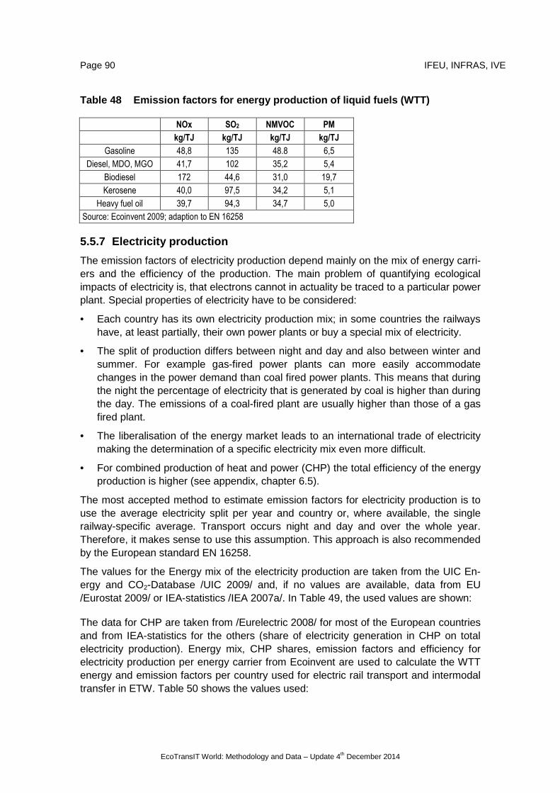
Page 90 IFEU, INFRAS, IVE
EcoTransIT World: Methodology and Data – Update 4th December 2014
Table 48 Emission factors for energy production of liquid fuels (WTT)
NOx SO2 NMVOC PM
kg/TJ kg/TJ kg/TJ kg/TJ
Gasoline 48,8 135 48.8 6,5
Diesel, MDO, MGO 41,7 102 35,2 5,4
Biodiesel 172 44,6 31,0 19,7
Kerosene 40,0 97,5 34,2 5,1
Heavy fuel oil 39,7 94,3 34,7 5,0
Source: Ecoinvent 2009; adaption to EN 16258
5.5.7 Electricity production
The emission factors of electricity production depend mainly on the mix of energy carri-ers and the efficiency of the production. The main problem of quantifying ecological impacts of electricity is, that electrons cannot in actuality be traced to a particular power plant. Special properties of electricity have to be considered:
• Each country has its own electricity production mix; in some countries the railways have, at least partially, their own power plants or buy a special mix of electricity.
• The split of production differs between night and day and also between winter and summer. For example gas-fired power plants can more easily accommodate changes in the power demand than coal fired power plants. This means that during the night the percentage of electricity that is generated by coal is higher than during the day. The emissions of a coal-fired plant are usually higher than those of a gas fired plant.
• The liberalisation of the energy market leads to an international trade of electricity making the determination of a specific electricity mix even more difficult.
• For combined production of heat and power (CHP) the total efficiency of the energy production is higher (see appendix, chapter 6.5).
The most accepted method to estimate emission factors for electricity production is to use the average electricity split per year and country or, where available, the single railway-specific average. Transport occurs night and day and over the whole year. Therefore, it makes sense to use this assumption. This approach is also recommended by the European standard EN 16258.
The values for the Energy mix of the electricity production are taken from the UIC En-ergy and CO2-Database /UIC 2009/ and, if no values are available, data from EU /Eurostat 2009/ or IEA-statistics /IEA 2007a/. In Table 49, the used values are shown:
The data for CHP are taken from /Eurelectric 2008/ for most of the European countries and from IEA-statistics for the others (share of electricity generation in CHP on total electricity production). Energy mix, CHP shares, emission factors and efficiency for electricity production per energy carrier from Ecoinvent are used to calculate the WTT energy and emission factors per country used for electric rail transport and intermodal transfer in ETW. Table 50 shows the values used:

IFEU, INFRAS, IVE Page 91
EcoTransIT World: Methodology and Data – Update 4th December 2014
Table 49 Energy split of electricity consumption
Source Ref. Year
Solid
fuels Oil Gas Nuclear
Renew-
able Other
Africa default /IEA 2007a/ 2006 42.4% 9.9% 27.9% 2.0% 17.9% 0.0%
South Africa /IEA 2007a/ 2006 92.6% 0.0% 0.0% 4.7% 2.7% 0.0%
Asia default /IEA 2007a/ 2006 45.2% 9.4% 24.2% 3.6% 17.2% 0.4%
China /IEA 2007a/ 2006 79.4% 1.8% 0.2% 1.9% 16.4% 0.3%
Hong Kong /IEA 2007a/ 2006 68.0% 0.3% 31.7% 0.0% 0.0% 0.0%
India /IEA 2007a/ 2006 67.2% 4.2% 8.3% 2.5% 17.5% 0.3%
Japan /IEA 2007a/ 2006 26.6% 10.7% 20.6% 27.5% 10.9% 3.6%
South Korea /IEA 2007a/ 2006 37.3% 5.8% 15.8% 37.0% 1.5% 2.6%
Australia default /IEA 2007a/ 2006 35.8% 8.0% 18.3% 25.1% 9.8% 3.0%
Australia /IEA 2007a/ 2006 78.3% 0.9% 11.7% 0.0% 8.3% 0.8%
South America default /IEA 2007a/ 2006 3.0% 10.5% 12.2% 2.2% 71.7% 0.5%
Brazil /IEA 2007a/ 2006 2.3% 2.8% 3.4% 3.1% 87.5% 0.8%
Europe default /IEA 2007a/ 2006 42.6% 5.7% 7.9% 14.8% 28.7% 0.3%
Austria /UIC 2009/ 2007 0.0% 0.0% 0.0% 0.0% 89.2% 10.8%
Belgium /UIC 2009/ 2007 13.6% 0.0% 16.6% 57.9% 2.1% 9.7%
Bulgaria /UIC 2009/ 2007 56.7% 1.0% 3.9% 29.2% 9.2% 0.0%
Cyprus /Eurostat 2009/ 2007 0.0% 100.0% 0.0% 0.0% 0.0% 0.0%
Czech Republic /UIC 2009/ 2007 57.3% 0.0% 0.0% 40.7% 2.0% 0.0%
Denmark /UIC 2009/ 2007 49.4% 2.7% 17.5% 0.0% 26.0% 4.4%
Estonia /Eurostat 2009/ 2007 93.4% 0.3% 5.0% 0.0% 1.3% 0.0%
Finland /UIC 2009/ 2007 0.0% 0.0% 0.0% 26.3% 32.4% 41.3%
France /UIC 2009/ 2005 4.0% 1.8% 3.3% 85.6% 4.9% 0.4%
Germany /UIC 2009/ 2007 46.0% 0.0% 8.8% 29.9% 14.0% 1.4%
Greece /Eurostat 2009/ 2007 53.8% 15.0% 22.3% 0.0% 9.0% 0.0%
Hungary /UIC 2009/ 2007 18.0% 1.5% 38.7% 36.5% 4.6% 0.7%
Iceland /Eurostat 2009/ 2006 0.0% 0.0% 0.0% 0.0% 100.0% 0.0%
Ireland /Eurostat 2009/ 2007 26.3% 6.8% 55.4% 0.0% 11.5% 0.0%
Israel /IEA 2007a/ 2006 68.8% 13.0% 18.2% 0.0% 0.1% 0.0%
Italy /UIC 2009/ 2007 29,8% 15,7% 0,0% 0,0% 29,3% 25,2%
Latvia /Eurostat 2009/ 2007 0.0% 0.3% 39.7% 0.0% 60.0% 0.0%
Lithuania /Eurostat 2009/ 2007 0.1% 2.8% 17.4% 69.6% 8.3% 1.7%
Luxembourg /Eurostat 2009/ 2007 0.0% 0.0% 71.9% 0.0% 28.1% 0.0%
Malta /Eurostat 2009/ 2007 0.0% 100.0% 0.0% 0.0% 0.0% 0.0%
Netherlands /UIC 2009/ 2005 23.3% 0.0% 51.8% 9.1% 9.7% 6.1%
Norway /UIC 2009/ 2007 0.0% 0.0% 0.0% 0.0% 100.0% 0.0%
Poland /UIC 2009/ 2005 93.7% 0.0% 1.9% 0.0% 0.0% 4.4%
Portugal /Eurostat 2009/ 2007 25.3% 10.0% 28.0% 0.0% 36.7% 0.0%
Romania /UIC 2009/ 2007 40.5% 1.1% 17.7% 13.0% 26.9% 0.9%
Slovakia /UIC 2009/ 2007 14.2% 0.0% 0.0% 66.0% 19.8% 0.0%
Slovenia /UIC 2009/ 2007 48.2% 1.0% 6.2% 30.0% 13.6% 1.0%
Spain /UIC 2009/ 2007 25.1% 0.8% 24.7% 19.5% 29.1% 0.8%
Sweden /UIC 2009/ 2007 0.0% 0.0% 0.0% 0.0% 100.0% 0.0%
Switzerland /UIC 2009/ 2007 0.0% 0.0% 0.0% 26.5% 73.5% 0.0%
Turkey /Eurostat 2009/ 2007 26.4% 3.3% 50.0% 0.0% 19.7% 0.6%
United Kingdom /UIC 2009/ 2007 33.1% 1.0% 43.7% 14.9% 5.3% 2.1%
North America default /IEA 2007a/ 2006 16.3% 1.5% 5.4% 15.5% 61.3% 0.0%
United States /IEA 2007a/ 2006 48.6% 1.8% 19.8% 19.0% 10.0% 0.8%
FSU default /IEA 2007a/ 2006 20.3% 2.9% 40.1% 17.5% 17.7% 1.5%
Russian Federation /IEA 2007a/ 2006 17.3% 2.4% 44.6% 15.5% 18.3% 1.9%

Page 92 IFEU, INFRAS, IVE
EcoTransIT World: Methodology and Data – Update 4th December 2014
Table 50 Energy and emission factors of the electri city supply for railway transport (WTT)
EC CO2e CO2 NOx SO2 NMVOC PM10
MJ/MJ g/MJ g/MJ g/MJ g/MJ g/MJ g/MJ
Africa default 2.24 223 207 0.431 0.643 0.048 0.040
South Africa 2.76 307 282 0.627 0.924 0.028 0.068
Asia default 2.29 227 212 0.429 0.716 0.044 0.046
China 2.12 326 277 1.040 2.303 0.013 0.210
Hong Kong 2.71 289 267 0.531 0.706 0.047 0.052
India 2.25 246 227 0.490 0.771 0.031 0.055
Japan 2.51 171 161 0.327 0.532 0.034 0.034
South Korea 2.61 169 157 0.331 0.511 0.030 0.034
Australia default 2.55 191 181 0.341 0.696 0.035 0.047
Australia 2.53 288 270 0.499 1.022 0.029 0.077
South America default 0.85 66 63 0.139 0.271 0.024 0.014
Brazil 0.45 26 26 0.048 0.118 0.007 0.009
Europe default 2.20 193 189 0.261 1.012 0.019 0.076
Austria 0.29 33 31 0.026 0.022 0.002 0.007
Belgium 2.86 109 106 0.214 0.367 0.015 0.029
Bulgaria 2.41 183 169 0.372 0.544 0.020 0.040
Cyprus 2.83 272 264 0.847 2.028 0.119 0.063
Czech Republic 2.21 184 182 0.289 0.344 0.005 0.016
Denmark 0.78 120 108 0.122 0.221 0.016 0.012
Estonia 2.84 336 331 0.389 1.847 0.013 0.146
Finland 1.84 133 126 0.142 0.502 0.007 0.038
France 2.78 21 20 0.062 0.088 0.007 0.007
Germany 2.09 159 146 0.136 0.117 0.015 0.012
Greece 3.45 279 272 0.317 1.231 0.038 0.172
Hungary 3.16 177 164 0.208 0.227 0.072 0.014
Iceland 0.15 3 3 0.008 0.008 0.002 0.005
Ireland 2.32 216 204 0.321 0.660 0.060 0.033
Israel 2.77 300 278 0.611 0.978 0.051 0.061
Italy 1.17 132 129 0.304 0.428 0.044 0.028
Latvia 0.43 44 42 0.051 0.020 0.019 0.004
Lithuania 2.29 30 28 0.048 0.055 0.014 0.004
Luxembourg 2.89 205 192 0.223 0.071 0.087 0.007
Malta 2.83 272 264 0.847 2.029 0.119 0.063
Netherlands 1.52 138 134 0.190 0.148 0.019 0.013
Norway 0.42 2 2 0.005 0.002 0.001 0.004
Poland 2.56 301 283 0.486 1.319 0.014 0.084
Portugal 1.53 151 145 0.401 0.856 0.045 0.029
Romania 1.70 154 151 0.184 0.724 0.016 0.058
Slovakia 2.45 55 55 0.110 0.605 0.003 0.058
Slovenia 2.26 191 188 0.447 3.097 0.011 0.082
Spain 1.63 118 111 0.357 0.567 0.018 0.046
Sweden 0.10 1 1 0.004 0.002 0.001 0.004
Switzerland 0.84 1 1 0.005 0.003 0.001 0.003
Turkey 2.10 201 192 0.264 0.576 0.048 0.043
United Kingdom 1.97 173 163 0.290 0.369 0.021 0.027
North America default 2.64 215 203 0.395 1.136 0.043 0.020
United States 2.64 215 203 0.395 1.136 0.043 0.020
FSU default 2.23 162 152 0.247 0.364 0.043 0.026
Russian Federation 1.68 127 120 0.182 0.276 0.035 0.020
Sources: /Eurelectric 2007/, /IEA 2007a/, /IEA 2007b/, /IEA 2008/;Emission Factors: /Ecoinvent 2009/

IFEU, INFRAS, IVE Page 93
EcoTransIT World: Methodology and Data – Update 4th December 2014
5.6 Intermodal transfer
Intermodal transfer can be relevant in a comparison of two transport variants, i.e. if one transport variant requires more transfer processes than the other. Therefore the trans shipping processes are classified in container, liquid, bulk and other cargo. On the ba-sis of assumptions and previous IFEU-studies, the energy use of the different transfer processes is estimated. All processes are performed with electricity. In addition to final energy consumption stated below, country specific energy and emission factors for electricity generation are used to produce Well-to-Wheels-values.
The European standard EN 16258 doesn’t considers up to now approaches for the calculations of energy consumption and GHG emission caused by intermodal transfers. This means that results for energy consumption and GHG emissions of transport ser-vices must not include intermodal transfers to be in accordance with EN 16258. Results for intermodal transfers are only additionally declared.
In the following the approaches for intermodal transfers of containers, liquid, bulk and other cargo are explained more in details:
Container: The energy used by a handling container in a rail cargo transport centre was estimated by /IFEU°2000/ with 4.4 kWh/TEU and transfer process. In previous studies /ISV1993, IFEU1999/ a lower value (2.2°kWh/°TEU+transfer) for rail was assessed. For container transfer in ship cargo transport centres, these studies searched out an energy fac-tor twice than rail /ISV°1993/. Because of high uncertainties, the value of 4.4 kWh/TEU+transfer is assumed for all carriers.
Liquid cargo: In /ISV°1993/ a very detailed calculation of the energy demanded by transhipping diesel was carried out. For different carriers the values range from 0.3 to 0.5 kWh/t, for which is why 0.4 kWh/t as average en-ergy use is assessed.
Bulk cargo: The results of early IFEU-estimations searching out the energy use of unloading corn from different means of transport were used in /ISV°1993/. For bulk cargo transfer the previous value 1.3 kWh/t is also used in EcoTransIT.
Other cargo: In this category all cargo, which is not container, liquid or bulk cargo is summarized. Thus the value for energy use of transhipping cargo of this category has the highest uncertainty. On basis of /ISV°1993/ a factor of 0.6 kWh/t for this category is taken.

Page 94 IFEU, INFRAS, IVE
EcoTransIT World: Methodology and Data – Update 4th December 2014
6 Appendix
6.1 EN 16258: Default conversion factors
Table 51 EN 16258 default values for fuels and gase s
density (d)
Energy factor CO2e-factor
MJ/kg kgCO2e/kg
Fuel type description kg/l TTW WTW TTW WTW
Gasoline 0,745 43,2 50,5 3,25 3,86 Ethanol 0,794 26,8 65,7 0,08 1,56 Diesel 0,832 43,1 51,3 3,21 3,9 Bio-diesel 0,890 36,8 76,9 0.08 2,16 Liquefied Petroleum Gas (LPG) 0,550 46,0 51,5 3,10 3,46 Compressed Natural Gas (CNG) x 45,1 50,5 2,68 3,07 Aviation Gasoline (AvGas) 0,800 44,3 51,8 3,13 3,76 Jet Gasoline (Jet B) 0,800 44,3 51,8 3,13 3,76 Jet Kerosene (Jet A1 and Jet A) 0,800 44,1 52,5 3,18 3,88 Heavy Fuel Oil (HFO) 0,970 40,5 44,1 3,15 3,41 Marine Diesel Oil (MDO) 0,900 43,0 51,2 3,24 3,92 Marine Gas Oil (MGO) 0,890 43,0 51,2 3,24 3,92
Table 52 Default values for carbon dioxide consiste nt with EN 16258
CO2-factor
kgCO2/kg
Fuel type description TTW WTW
Gasoline 3.17 3.78 Ethanol 0.00 0.75 Diesel 3.16 3.84 Bio-diesel 0.00 0.62 Liquefied Petroleum Gas (LPG) 3.02 3.37 Compressed Natural Gas (CNG) 2.54 2.78 Aviation Gasoline (AvGas) 3.10 3.74 Jet Gasoline (Jet B) 3.10 3.74 Jet Kerosene (Jet A1 and Jet A) 3.15 3.85 Heavy Fuel Oil (HFO) 3.11 3.38 Marine Diesel Oil (MDO) 3.21 3.89 Marine Gas Oil (MGO) 3.21 3.89

IFEU, INFRAS, IVE Page 95
EcoTransIT World: Methodology and Data – Update 4th December 2014
6.2 Example for an ETW declaration in accordance wi th EN 16258

Page 96 IFEU, INFRAS, IVE
EcoTransIT World: Methodology and Data – Update 4th December 2014
6.3 Additional information to load factors
In this chapter some explanations about the load factor of trains and containers are given in addition to chapter 3.2.2.
6.3.1 Train
The load factor for trains is originally defined as the relation of net tonnes / gross tonne. For a better comparison with road and ship transport the values are transformed to the relation freight load/capacity. The following figure shows a comparison of the load fac-tors for freight trains, based on the average wagon defined in ETW (see chapter 3.2.1: empty weight: 23 tonnes, payload capacity: 61 tonnes).
Figure 26 Load factors for freight trains
6.3.2 Container
Many cargoes shipped in containers are light weight consumer goods17. The emissions per TEU-km are allocated to the net-load of the container. Since emissions of container vessels are calculated on a g/TEU-km basis and energy consumption of the ship only marginally depends on the load of the container, volume and average weight cargo is
17 Container vessels’ carrying capacity by weight is usually achieved if all container spac-
es are used and containers weigh no more than 12 gross tonnes for large container vessels and 15 tonnes gross for small container vessels. Thus container vessels cannot be fully loaded with only heavy weight containers.
Load Factors Freight Train
0%
20%
40%
60%
80%
100%
120%
0 2 4 6 8 10 12 14 16 18 20 22 24 26 28 30 32 34 36 38 40 42 44 46 48 50 52 54 56 58 60
Load weight (t)
Load
fact
or
net-tons/gross-tonsnet-tons/capacity

IFEU, INFRAS, IVE Page 97
EcoTransIT World: Methodology and Data – Update 4th December 2014
responsible for higher emissions on a per tonne-kilometre basis than heavy weight car-go. Three container load classes and an average empty TEU weight are provided as default values (see Table 53).
Average cargo:
In accordance with the Clean Cargo Working Group (CCWG) the net weight of average goods is be defined by 10.0 tonnes per TEU /CCWG 2014/. Cargo is transported in 20’ and 40’ containers in the ratio of approximately 2 to 5, i.e. 2 TEU to 10 TEU18. Thus, for each lift19 an average of 1.7 TEUs is loaded. The average empty weight of a TEU is 1.95 tonnes20.
Volume cargo:
For determining the default volume cargo load of one TEU a convention was used. It is assumed that light weight cargo (volume cargo) tends to be transported in 40’ contain-ers. Generally, a maximum load of 90 % of the capacity is assumed due to imperfect fit of the cargo in the container. Then the light weight is assumed to be using 50 % of the carrying capacity. Thus, a 40’ Container filled 45 %21 to its weight carrying capacity is assumed to represent a light weight cargo container. These results in 6.0 tonnes/TEU and an average empty container weight of 1.9 tonnes.
Heavy weight cargo:
The default heavy weight TEU load is derived similarly. Here 90 % of the maximum carrying capacity of the containers is assumed to represent the heavy weight cargo. In order to determine the average heavy weight, the use of 20’ and 40’ containers for heavy weight cargo need to be determined. Applying the 1.7 ratio 40’ to 20’ container results in approximately 5x 40’ containers and 2x 20’ containers or 12 TEUs. In the set of 12 TEUs and 7 containers, a ratio of 3x 40’ containers filled with volume weight car-go and 2x 40’ containers plus 2x 20’ containers filled with heavy weight cargo result in the overall average weight of 10.5 tonnes. The heavy weight containers are then filled with 14.5 tonnes per TEU on average22 and an average empty container weight of 2.0 tonnes. A theoretical model container vessel is assumed to be loaded with
• x-number of average loaded containers (20’ and 40’)
• plus x-time the mix of 2x 20’ plus 2x 40’ heavy load and 3x 40’ light weight load.
18 A ratio of 1.7 was determined by comparing lifts and TEUs handled from port statistics.
19 Lift is an expression from container terminals and describes the number of containers loaded on-board of vessels.
20 Calculated from a mix of 20’ and 40’ containers.
21 50 % of the container weight capacity utilised to a maximum of 90 %.
22 Assuming a maximum utilisation by weight of 90 %.
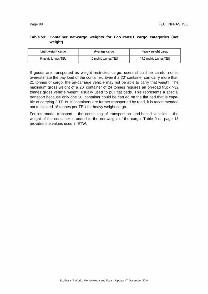
Page 98 IFEU, INFRAS, IVE
EcoTransIT World: Methodology and Data – Update 4th December 2014
Table 53: Container net-cargo weights for EcoTransI T cargo categories (net weight)
Light weight cargo Average cargo Heavy weight cargo
6 metric tonnes/TEU 10 metric tonnes/TEU 14.5 metric tonnes/TEU
If goods are transported as weight restricted cargo, users should be careful not to overestimate the pay load of the container. Even if a 20’ container can carry more than 21 tonnes of cargo, the on-carriage vehicle may not be able to carry that weight. The maximum gross weight of a 20’ container of 24 tonnes requires an on-road truck >32 tonnes gross vehicle weight, usually used to pull flat beds. This represents a special transport because only one 20’ container could be carried on the flat bed that is capa-ble of carrying 2 TEUs. If containers are further transported by road, it is recommended not to exceed 18 tonnes per TEU for heavy weight cargo.
For intermodal transport – the continuing of transport on land-based vehicles – the weight of the container is added to the net-weight of the cargo. Table 9 on page 13 provides the values used in ETW.

IFEU, INFRAS, IVE Page 99
EcoTransIT World: Methodology and Data – Update 4th December 2014
6.4 Detailed data of selected types of aircrafts
Table 54 Design range, payload and seats of selecte d types of aircrafts
Type Aircraft
Code Type of Aircraft
Design
Range [km]
Max. Pay-
load [t]
Typical
Seats
[number]
Freighter ABY Airbus 300-600F 4,850 48.1
Freighter 31Y Airbus 310-300F 5,560 39.1
Freighter 33X Airbus 330-200F 7,400 65.0
Freighter ATY ATR 72-200F 960 7.8
Freighter 14F BAe 146-300QT 1,930 12.5
Freighter M1F Boeing (McDonnell Douglas) MD-11F 6,700 89.6
Freighter 72F Boeing 727F 2,570 29.5
Freighter 73Y Boeing 737-300SF 3,030 19.7
Freighter 74X Boeing 747-200F 6,640 111.0
Freighter 74Y Boeing 747-400F 8,250 113.0
Freighter 74N Boeing 747-8F 8,130 133.9
Freighter 75F Boeing 757-200PF 5,830 32.8
Freighter 76X Boeing 767-200F 5,790 45.0
Freighter 77X Boeing 777-200F 8,410 102.9
Belly 319 Airbus 319 3,300 1.7 124
Belly 320 Airbus 320 5,700 2.4 150
Belly 321 Airbus 321 5,500 2.8 185
Belly 332 Airbus 330-200 12,500 17.5 253
Belly 333 Airbus 330-300 10,500 21.0 295
Belly 346 Airbus 340-600 13,900 22.0 380
Belly 388 Airbus 380-800 15,000 20.0 525
Belly M90 Boeing (McDonnell Douglas) MD-90 3,860 3.0 153
Belly 734 Boeing 737-400 4,010 3.5 147
Belly 738 Boeing 737-800 3,590 4.0 162
Belly 744 Boeing 747-400 13,450 16.8 416
Belly 74H Boeing 747-8i 14,820 17.4 467
Belly 752 Boeing 757-200 7,220 3.8 200
Belly 763 Boeing 767-300 10,310 13.7 218
Belly 772 Boeing 777-200/200ER 9,700 19.0 305
Belly 77W Boeing 777-300ER 14,490 23.0 365
Belly 788 Boeing 787-8 14,200 15.8 242
Belly E90 Embraer 190 3,330 1.4 98

Page 100 IFEU, INFRAS, IVE
EcoTransIT World: Methodology and Data – Update 4th December 2014
6.5 Allocation of electricity from CHP and its envi ronmental impacts
In some cases electricity for rail transport is produced in power plants producing both: electricity and heat (cogeneration or Combined Heat and Power - CHP). Therefore the environmental impacts of running the power plant have to be burdened (allocated) on both output products as well. Amongst others, the following allocation methodologies are feasible:
1. Allocation by Energy
2. Allocation by Exergy
3. Approach mentioned in /Directive 2004/8/EC/
The allocation by energy is based on the assumption, that one unit of heat is equivalent to one unit of electricity. This assumption is also the main disadvantage of this ap-proach, because in regards to thermodynamics electricity has a higher work potential than heat. So the more valuable product of cogeneration is electricity and actually has to be burdened with more environmental impact units than heat. Thus this allocation methodology favours electricity.
In contrast, the allocation by exergy is considering the different valence of electricity and heat. In /Heck 2004/ one unit electricity is equivalent to 0.17 unit heat. This meth-odology is favoured by scientific institutions (e. g. IFEU) but does not represent an ap-proved European standard for CHP allocation so far.
Compared to the allocation by exergy the approach mentioned in /Directive 2004/8/EC/ (also called “Finnish Methodology”) represents an European wide accepted methodol-ogy. It was developed to calculate the efficiency of new CHP power plants. Therefore the difference (reduction) between the production in CHP and the production in a sepa-rate heat and a separate electricity power plant is estimated. The default values for the separate production are defined by /Decision 2007/74/EC/. The methodology does not take the different valence of electricity and heat into account (cp. exergy). But electricity gets a lower environmental benefit compared to the allocation by energy. And this methodology is approved within the European Union. Thus we use this approach to allocate the environmental impacts of cogeneration.
The following table shows the effect of using the three described allocation methodolo-gies on the overall efficiency and CO2-emission factor:

IFEU, INFRAS, IVE Page 101
EcoTransIT World: Methodology and Data – Update 4th December 2014
Table 55 Comparison of different methodologies to a llocate environmental im-pacts of electricity from cogeneration
Denmark Germany
Efficiency of total electricity generation* w/o Allocation** 36% 30% 1. Energy 70% 33%
2. Exergy 43% 31%
3. Directive 2004/8/EC (Finnish Methodology) 56% 32%
Specific CO2-emissions of total electricity generation* [kg/kWh] w/o Allocation** 0,636 0,586 1. Energy 0,302 0,508
2. Exergy 0,524 0,558
3. Directive 2004/8/EC (Finnish Methodology) 0,390 0,527
* incl. electricity from CHP and conventional electricity generation (total electricity mix) ** electricity from CHP is estimated like non-CHP electricity (allocation factors: 100% electricity; 0% heat) Source: IFEU

Page 102 IFEU, INFRAS, IVE
EcoTransIT World: Methodology and Data – Update 4th December 2014
7 References
General
Borken 1999 Borken, J., Patyk, A., Reinhardt, Guido A., IFEU: Basisdaten für ökologische Bilanzierungen – Einsatz von Nutzfahrzeugen in Transport, Landwirtschaft und Bergbau; Verlag Vieweg, ISBN 3-528-03118-2; Braunschweig/Wiesbaden 1999
Carstens 2000 Stefan Carstens, Hans Ulrich Diener: Güterwagen Band 2, Gedeckte Wagen - Sonderbauart. MIBA-Verlag, Nürnberg 2000; citation in: http://en.wikipedia.org/wiki/Covered_goods_wagon
DB Schenker 2012 Internal survey: key values of freight transport from railway transport statis-tics, 2012
GDV 2010 Containerhandbuch / Container Handbook. Gesamtverband der Deutschen Versi-cherungswirtschaft e.V. http://www.containerhandbuch.de/
IFEU 1999 Knörr, W. et al.: Mobilitäts-Bilanz – Energieverbrauch und Emissionen im Perso-nen- und Güterverkehr mit verschiedenen Verkehrsmitteln; Erstellung verschiedener Materialien und Tools im Auftrag der DB AG; 1998 - 2000; Veröffentlichung der “Mobili-täts-Bilanz“ und der Software „Reisen und Umwelt“ im Okt. 1999
KBA 2002 Güterkraftverkehr deutscher Lastkraftfahrzeuge; Reihe 8, Heft 12, Dezember 2001
KBA 2013 KBA and BAG: Verkehr deutscher Lastkraftfahrzeuge; VD5, Dezember 2013
Kessel und Partner 1998 Kienzler, H.-P.: Kapazitätsauslastung und Leerfahrten im Güter-transport; VDA Materialien zur Automobilindustrie, Heft 16; Frankfurt am Main 1998
SNCF Geodis 2012 Internal survey: key values of freight transport from railway transport statis-tics, 2012
Van de Reyd and Wouters Van de Reyd, J.K.R., Wouters, M.V.L.J.: Air Cargo Density Re-search. Delft 2005
Road transport
Dieselnet 2014 DieselNet - Online information service on clean diesel engines and diesel emissions: Summary of worldwide emission standards, http://www.dieselnet.com, last visit October 10th, 2014
EPA 2009 Motor Vehicle Emission Simulator (MOVES), Version 2009/12/21, by EPA Office for Transportation and Air Quality, retrieved from, http://www.epa.gov/otaq/models/moves/
INFRAS 2014 Keller, M. et al, INFRAS, et al: Handbook Emission Factors for Road Transport, Ver. 3.2, Bern 2014
USCB 2004 U.S. Census Bureau - 2002 Economic Census: Vehicle Inventory and Use Survey (VIUS); EC02TV-US, Washington DC, 2004
USDOE 2009 U.S. Departement of Energy: Transportation Energy Data Book, Edition 28, 2009
USDOT 2007 U.S. Departement of Transport – Federal Highway Administration: Development of Truck Payload Equivalent Factor (TPEF), Columbus, 2007
Rail transport
DB 2008 Deutsche Bahn AG, Bahn-Umwelt-Zentrum: Energy and emission figures 2008

IFEU, INFRAS, IVE Page 103
EcoTransIT World: Methodology and Data – Update 4th December 2014
DB Schenker 2012 Internal survey: key values of freight transport from railway transport statis-tics, 2012
EPS 2005 Railway Association of Canada and Environment Canada: Locomotive Emissions Monitoring Program 2003; Environmental protection series: EPS 2/TS/17; 2005
IFEU 2008 Sectoral analysis of motorised traffic in China; commissionned by Kreditanstalt für Wiederaufbau (KfW); Heidelberg, 2008
Railion 2007 Internal survey: energy consumption of freight trains; 2007
Railway companies 2002 Different internal statistics DB, DSB, SBB, SJ, SNCB, SNCF und TI about railway operation data, energy consumption, train configuration etc., 2002
SBB 2006 Enotrac AG: Simulationsrechnungen für Re 420 und Re 620; unpublished; March 2006
SNCF Geodis 2012 Internal survey: key values of freight transport from railway transport statis-tics, 2012
TRT 2008 TRT Trasporti e Territorio Srl: EX-TREMÌS (Exploring non road Transport EMISsions in Europe): Development of a Reference System on Emission Factors for Rail, Maritime and Air Transport; Final Report; commissionned by JRC-IPTS; Milan, 19 June 2008
UIC 2005 UIC/CER: Rail Diesel Study (EU funded) - WP1: Status and future development of the diesel fleet; Final Report; 21.07.2005
UIC 2007 UIC Statistic
UIC 2009 UIC Energy and CO2 Database; 2009
USDOT 2008 Energy Intensity of Class I Railroad a Freight Service
Inland ship and Marine transport
AKN 2009 Aktionskonferenz Nordsee: Klimaschutz im Seeverkehr. Februar 2009.
Aldrete, G. et al. 2005 Port of Los Angeles Baseline Emission Inventory 2001. Prepared by Starcrest Consulting Group. Los Angeles 2005.
Anderson, B. et al. 2003 The New York, Northern New Jersey, Long Island Nonattainment Area Commercial Marine Vessel Emissions Inventory. Prepared by Starcrest Consulting Group. The Port Authority of New York/New Jersey and the United States Army Corps of Engineers, New York District.
Anderson, B. et al. 2004 Port of Long Beach Baseline Emission Inventory 2002. Prepared by Starcrest Consulting Group. Long Beach 2004.
BVB 2009 The power of inland navigation. The future of freight transport and inland shipping in Europe 2010 – 2011. Published by the Dutch Inland Shipping Information Agency (BVB).
CARB 2006 Emission Estimation Methodology for Ocean Going Vessels. Draft. OGV Working Group 10/4/05, California Air Resources Board.
Caterpillar 2006 Marine engine selection guide. Caterpillar Marine Power Systems.
CCWG 2014 Clean Cargo Working Group (CCWG): Global Maritime Trade Lane Emissions Factors. August 2014.
Corbett J.J. and Fischbeck P.S. 1997 “Emissions from Ships”. Science. 278 (5339), 823–824, doi:10.1126/science.278.5339.823.
Corbett, J.J. 2004 Verification of Ship Emission Estimates with Monitoring Measurement to Improve Inventory and Modeling. Final Report prepared for the California Air Resources Board and Environmental Protection Agency.
Corbett, J.J. and Köhler, H.W. 2003 “Updated emissions from ocean shipping”. J. Geophys. Res. 108 (D20), 4650, doi:10.1029/2003JD003751.

Page 104 IFEU, INFRAS, IVE
EcoTransIT World: Methodology and Data – Update 4th December 2014
ENTEC 2002 Quantification of emissions from ships associated with movements between ports in the European Community. Final Report issued for the European Commission. July 2002. London.
EPA 2006 Current Methodologies and Best Practices in preparing Port Emission Inventories. Prepared by ICF Consultants. Final Report. January 5, 2006.
Gohlisch, G.; Huckestein, B.; Naumann, S.; Röthke-H abeck, P. 2005 Umweltauswirkungen der Binnenschifffahrt. In: Internationales Verkehrswesen (57) 4/2005.
Günthner et al. 2001 Studie Donau Logistik. Technische und logistische Maßnahmen zur weiteren Entwicklung der Verkehre über die deutschen und österreichischen Do-nauhäfen. Prof. W. Günthner, H. Segerer, M. Heinecker, Lehrstuhl für Fördertechnik, Materialfluß und Logistik der TU München. Bericht im Auftrag des Freistaats Bayerns. Garching 2001.
HELCOM 2007 Recommendation 28/E13: Introducing economic incentives as a complement to existing regulations to reduce emissions from ships. Adopted 15 November 2007. Hel-sinki Convention. http://www.helcom.fi/Recommendations/en_GB/rec28E_13/
IMO 2000 Study of Greenhouse Gas Emissions from Ships. Kjell Olav Skjølsvik, Aage Bjørn Andersen, James J. Corbett, John Magne Skjelvik. Norwegian Marine Technology Re-search Institute (MARINTEK) prepared for the IMO. MT Report: MT00 A23-038, Trond-heim, Norway, March 2000.
IMO 2009 Second IMO GHG Study 2009: International Maritime Organisation (IMO) London, UK, April 2009; Buhaug, Ø.; Corbett, J.J.; Endresen, Ø.; Eyring, V.; Faber, J.; Hanaya-ma, S.; Lee, D.S.; Lee, D.; Lindstad, H.; Markowska, A.Z.; Mjelde, A.; Nelissen, D.; Nil-sen, J.; Pålsson, C.; Winebrake, J.J.; Wu, W.–Q.; Yoshida, K..
IPCC 2006 2006 IPCC Guidelines for National Greenhouse Gas Inventories. Volume 2: Ener-gy. Edited by Simon Eggelston, Leandro Buendia, Kyoko Miwa, Todd Ngara, and Kiyoto Tanabe. Intergovernmental Panel on Climate Change (IPCC) National Greenhouse Gas Inventories Programme.
Lindhjem 2004 LADCO non-road emission inventory project for locomotive, commercial ma-rine, and recreational marine emission sources. Final report. ENVIRON Consultants prepared for Lake Michigan Air Director Consortium (LADCO)
Lloyds 2009 Lloyds register of ships 2009/2010. Lloyds Register Fairplay. London 2009. Vol-ume 1 – 4.
MAN 2006 Basic Principles of Ship Propulsion. Technical Paper by MAN DW.
MEPC 2009 Guidelines for voluntary use of the Ship Energy Efficiency Operational Indicator (EEOI). MEPC.1/Circ.684. 17 August 2009.
MEPC 2009b Prevention of Air Pollution from Ships, Sulphur monitoring for 2008. Note by the Secretariat, Marine Environmental Protection Committee, 59th Session, MEPC 59/4/1, 3 February 2009.
Planco 2007 Verkehrswirtschaftlicher und ökologischer Vergleich der Verkehrsträger Straße, Schiene und Wasserstraße. Schlussbericht, November 2007. Planco Consulting in Zusammenarbeit mit Bundesanstalt für Gewässerkunde, im Auftrag der Wasser- und Schifffahrtsverwaltung des Bundes.
Seum 2010 Seum, S.: Detailed description of the ETW methodology for emission factors of ocean-going vessels. Berlin: 2010.
Sustainable Shipping 2009 Emission Control Areas (ECAs) – What you need to know. A Sus-tainable Shipping Briefing Paper, August 2009.
UNECE 1996 European Agreement on Main Inland Waterways of International Importance (AGN). United Nations Economic Commission for Europe, Geneva 19 January 1996.

IFEU, INFRAS, IVE Page 105
EcoTransIT World: Methodology and Data – Update 4th December 2014
Ferries Bäckström 2003 °°Bäckström, S.: Internal description of the proposed NTM-methodology and
comments to the proposal for EcoTransIT; February 2003
Kristensen 2000 H.O. H. Kristensen (Danish Shipowners Association: Energy consumption and exhaust emissions for various types of marine transport compared with trucks and private cars; paper presented at ENSUS 2000 conference - newcastele 4-6 September 2000
Kusche 2000 Kusche, J.: Transport-Ökobilanz von Deutschland nach Schweden; Diplomarbe-it, Berlin 2000
TT-Lines 2009 Internal values for energy consumption, capacity and load factor from TT Lines, 2009
Aircraft transport
Airbus 2013 Airbus (Ed.): Future payloads - freight forecast 2013 - 2032; Blagnac Cedex (France) 2013
Atmosfair 2009 Atmosfair (Ed.): The atmosfair emission calculator. Methodological back-ground. Berlin: 2009
DECC 2014 Department of Energy and Climate Change (DECC): 2014 Government GHG Conversion Factors for Company Reporting: Methodology Paper for Emission Factors / Hill, N.; Dun, C.; Watson, R. (Ricardo-AEA); James, K. (WRAP). Report on behalf of the Department of Energy and Climate Change (DECC) and the Department for Environ-ment, Food and Rural Affairs (Defra). London: 2014
EEA 2013 EEA (European Environment Agency): EMEP/EEA Air pollutant emission inventory guidebook 2013. Technical guidance to prepare national emission inventories. EEA Technical report No 12/2013. Copenhagen: 2013
EUROCONTROL 2009 Astorino, A.: EUROCONTROL ETS Support Facilities and Fuel Estimator tool. Presentation. Brussels: 2009
EUROCONTROL 2013a EUROCONTROL: Small emitters tool: Version 5.01_2 dated 2013.03.06. Brussels: 2013
EUROCONTROL 2013b EUROCONTROL: Standard Inputs for EUROCONTROL Cost Benefit Analyses. Edition Number: 6.0. Edition Date: September 2013. Brussels: 2013
Hünecke 2008 Hünecke, K.: Die Technik des modernen Verkehrsflugzeuges. Stuttgart: Motor-buch Verlag 2008
Graßl/Brockhagen 2007 Graßl, H; Brockhagen, D.: Climate forcing of aviation emissions in high altitudes and comparison of metrics. An update according to the Fourth Assess-ment Report, IPCC 2007. Hamburg: 2007
IATA 2013 International Air Transport Association (IATA): Cargo e-Chartbook – Q2 2013.
ICAO 2012 International Civil Aviation Organisation (ICAO): ICAO Carbon Emissions Calcula-tor. Version 5. Montreal: 2012
IFEU 2010 Knörr, W. (IFEU-Institut): EcoPassenger: Environmental Methodology and Data. Final Report. Commissioned by International Union of Railways (UIC). Heidelberg: 2010
IFEU/Öko-Institut 2012: Knörr, W.; Schacht, A. (IFEU); Gores, S. (Öko-Institut): Entwicklung eines Modells zur Berechnung der Energieeinsätze und Emissionen des zivilen Flu-gverkehrs – TREMOD AV. UBA-Texte, No. 48/2012. Dessau: 2012
IPCC 1999 Intergovernmental Panel on Climate Change (IPCC): Aviation and the Global At-mosphere. A Special Report of IPCC Working Groups I and III in collaboration with the Scientific Assessment Panel to the Montreal Protocol on Substances that Deplete the Ozone Layer. Cambridge: University Press, 1999.

Page 106 IFEU, INFRAS, IVE
EcoTransIT World: Methodology and Data – Update 4th December 2014
IPCC 2006 Intergovernmental Panel on Climate Change (IPCC): Datenbank für Emis-sionsfaktoren vom IPCC. 2006. See http://www.ipcc-nggip.iges.or.jp/EFDB/main.php.
Lang 2007 Lang, G.: Passagierflugzeuge – Das aktuelle Typenbuch. München: Scont-Verlag, 2007
Lang 2009 Lang, G.: Flugzeuge – Die bekanntesten Passagierflugzeuge der Welt. Fränkisch-Crumbach: Edition XXL, 2009
Lufthansa 2014 Deutsche Lufthansa AG (Ed.): Geschäftsbericht 2013. Frankfurt/M.: 2014.
LCAG 2014 Lufthansa Cargo (Ed.): Pallets, Container and Fleet. Frankfurt/M.: 2014
Öko-Institut 2009 Graichen, J.; Gores, S.; Herold, A.: Überarbeitung des Emissionsinventars des Flugverkehrs. Final report on behalf of the Umweltbundesamtes. Berlin: 2009
Piano 2008 Pianox: Aircraft Emissions and Performance User’s Guide. Woodhouse Eaves (UK): 2008
UBA 2008 Umweltbundesamt (2008): Klimawirksamkeit des Flugverkehrs. Aktueller wissen-schaftlicher Kenntnisstand über die Effekte des Flugverkehrs. Dessau: März 2008.
Energy supply
Eurelectric 2007 Statistics and prospects for the European electricity sector - EURPROG 2007; Bruxelles, October 2007
Eurostat 2009 Yearly Energy Statistics – 2007 Data
Heck 2004 Wärme-Kraft-Kopplung. In: Dones, R. (Ed.) et al., Sachbilanzen von Energie-systemen: Grundlagen für den ökologischen Vergleich von Energiesystemen und den Einbezug von Energiesystemen in Ökobilanzen für die Schweiz. Final report ecoinvent 2000 No. 6-V, Paul Scherrer Institut Villigen, Swiss Centre for Life Cycle Inventories, Dübendorf, CH. Online: www.ecoinvent.org
IEA 2007a IEA Energy Statistics - Electricity/Heat, last update 8/2009
IEA 2007b IEA Electricity Information 2007, Paris, 2007
IEA 2008 Combined Heat and Power, Paris, 2008
UIC 2009 UIC Energy and CO2 Database, Paris, 2009
UNEP 2014 Partnership for Clean Fuels and Vehicles – Diesel Fuel Sulphur Levels: Global Status April 2014; http://www.unep.org/transport/new/pcfv/pdf/Maps_Matrices/world/sulphur/MapWorldSulphur_april2014.pdf ; last visit October 10th, 2014
SBB 2008 Verkehrsträgervergleich v2.0: Lebenswegbezogene Umwelt- und Energiekennwerte von Verkehrsleistungen. BahnUmwelt-Center der Schweizerischen Bundesbahnen (SBB): Markus Halder, ESU-services GmbH: Matthias Tuchschmid, Bern, Switzerland.
Directive 2004/8/EC Directive 2004/8/EC of the European Parliament and of the Council of 11 February 2004 on the promotion of cogeneration based on a useful heat demand in the internal energy market and amending Directive 92/42/EEC
Decision 2007/74/EC Decision of 21 December 2006 establishing harmonised efficiency refer-ence values for separate production of electricity and heat in application of Directive 2004/8/EC of the European Parliament and of the Council (notified under document number C(2006) 6817)
Ecoinvent 2009 °ecoinvent Centre (2009): ecoinvent data v2.1. Final reports ecoinvent data v2.1. Swiss Centre for Life Cycle Inventories, Dübendorf, 2009, retrieved from: http://www.ecoinvent.org

IFEU, INFRAS, IVE Page 107
EcoTransIT World: Methodology and Data – Update 4th December 2014
Intermodal transfer
IFEU 2000 Knörr, W. et. al, IFEU and SGKV (Studiengesellschaft für den kombinierten Verkehr e.V).: Comparative Analysis of Energy Consumption and CO2 Emissions of Road Transport and Combined Transport Road/Rail; comissioned by IRU (International Road Union) and BGL (Bundesverband Güterkraftverkehr Logistik und Entsorgung e.V.); Geneva/Frankfurt a.M. 2002
ISV 1993 Systemvergleich für unterschiedliche verkehrliche Prozessabläufe/Transportketten hinsichtlich Energieeinsatz und klimarelevanter Emissionen (im Güterverkehr). Bearbeitet von ISV (Uni Stuttgart), IER (Uni Stuttgart), ISB (Uni Hannover) und IFEU im Auftrag der Enquête-Kommission "Schutz der Erdatmosphäre" des Deutschen Bundes-tages, 1993.

Page 108 IFEU, INFRAS, IVE
EcoTransIT World: Methodology and Data – Update 4th December 2014
8 Expressions and abbreviations Gtkm Gross tonne kilometre hauled Tonne kilometre of freight including empty wagon (vehicle, vessel)
weight; for railways: train without locomotive
Ntkm Net tonne kilometre: Tonne kilometre of freight; also: tkm
tkm Tonne kilometre Tonne kilometre of freight; also: Ntkm (in distinction to Gtkm)
Gt Gross tonnes t Tonnes of freight including empty wagon (vehicle, vessel) weight; for railways: train without locomotive
Nt Net tonnes Tonnes of freight
T Tonne Metric tonne, unit used in ETW for the freight mass
RFI Radiative Forcing Index Takes into account the climate effects of other GHG emissions (in particular nitrogen oxides, ozone, water, soot, sulphur), especially for emissions in high altitudes. (>9km)
Payload Load weight of freight
CP Payload capacity Mass related capacity of a vehicle/vessel for freight
LF Load factor Relation of net tonnes and tonne capacity of a vehicle/vessel without empty trip factor
CU Capacity utilisation Relation of net tonnes and tonne capacity of a vehicle/vessel including the empty trip factor
ET Empty trip factor Relation of vehicle/vessel-km running empty and km loaded
D Distance Transport distance in km
Km Kilometre
M Mass of freight
EC Energy consumption
ECT Total energy consumption Sum of final energy consumption and upstream energy consump-tion
ECF Final energy consumption Energy consumption of vehicle/vessel
ECU Upstream energy consumption Energy consumption for production and delivery of final energy
EGR Exhaust Gas Recirculation Technology to reduce emissions of diesel engines
EMT Total emissions Sum of vehicle and upstream emissions
EMV Emissions vehicle Direct emissions from vehicle operation
EMU Upstream Emissions Emissions of upstream process
HFO Heavy fuel oil Fuel for marine vessels
MDO Marine diesel oil
MGO Marine Gas oil
SCR Selective Catalytic Reduction Technology to reduce emissions of diesel engines
TEU Twenty foot equivalent Unit for container transport
TTW Tank-to Wheels Energy consumption and emissions from vehicle operation
WTT Well-to-Tank Energy consumption and emissions from upstream processes
WTW Well-to-Wheels Energy consumption and emissions from vehicle operation and upstream processes