Embed Size (px)
Citation preview

Middle East Technical University
Electrical & Electronics Engineering Department
EE 426 Antennas and Propagation
Laboratory Manual

Contents
SUP#1 Report Format and Remarks
SUP#2 Introduction to Antenna Experiments
EXP#1 Radiation Pattern and Gain Measurements of Antennas
in Anechoic Chamber
EXP#2 Radiation Pattern Measurements of Antennas
EXP#3 Polarization Pattern and Bandwidth Measurements of Antennas
EXP#4 Linear Antennas: Impedance & Pattern Measurements
EXP#5 Reflection Method for Gain Measurements
EXP#6 Electromagnetic Fields: Measurements and Aperture Field Shaping
EXP#7 Antenna Arrays

Experiment EE426-0 Lab Report Format and Remarks
Middle East Technical University i.1 Dept. of Electrical & Electronics Eng.
EE426AntennasandPropagationLaboratory
ReportFormatandRemarks
GeneralRemarksaboutLaboratorySessions
• Each student is viewed as a responsible professional in engineering, and thus highest ethical
standards are presumed.
• It is obligatory to prepare the preliminary work in order to start an experiment. Note that
doing the preliminary work means completing a considerable portion of it, preliminary work
with negligent and insufficient content cannot be accepted.
• Be punctual, laboratory sessions are strictly 4 hours. Together with your partner(s), you are
responsible to perform all the steps of the experiment, i.e. all the partners should be ready at
each laboratory session.
• All students are required to read the whole manual of the experiment, and are also assumed
they have done so, before attending the session. This is of great significance to successfully
complete the experiment, and to comprehend the main purpose. Remember that you are
always encouraged to ask what you want to know further or what you do not understand,
before/during/after the experiments.
• There will be a quiz at the end of each experiment and time allocated for the quiz is 10
minutes. Remember that doing the preliminary work on your own is the key point to be
ready for the quiz and have a successful laboratory session.
• Take a copy of your preliminary work before submitting it; you will need it while writing your
report.

Experiment EE426-0 Lab Report Format and Remarks
Middle East Technical University i.2 Dept. of Electrical & Electronics Eng.
Report Format
• The reports must be typed using a word-processor software.
• Do not forget to include the following in the header of the report document:
Name and number of the experiment together with the course name,
Date of the session and the date of the report,
Names, student IDs of the students.
• Please reduce paper consumption:
Do not use a cover page.
Print your reports using both sides of the papers.
• Your report will include the following parts:
Introduction: The purpose of this part is to generally summarize your past session. Here are
what you need to write:
Briefly explain the aim of the experiment.
Summarize the procedure, measurements and the methods used. Do not tabulate your
measurements here.
Results and Comments: The content is generally directed by the manual. Please note the
following:
Follow the same steps with the corresponding part of the manual.
Tabulate your results and draw necessary graphs. Also point out the results you observe
from the figures and/or tables.
Make comparisons of the results with the preliminary work where applicable.
State any results contradicting or matching your expectations. Discuss the results you
obtained (both expected and unexpected results).
Please comment about what you put forward as a result.
Conclusion: You are expected to sum up the whole idea of the experiment. In addition:
Write a general discussion of what you have learned.
Specifically point out the differences between ideal/theoretical cases and the practical
aspects, express your reasoning briefly.
• Label the figures and tables you include with an appropriate name and number.
• Please think of these reports as a team work. All group members are responsible from the
reports and are expected to participate in preparing them. This is a necessity not only to behave
ethically; but also to comprehend the whole laboratory process.
• Please keep this document at hand while writing the reports.

Experiment EE426-0 Introduction to Antenna Experiments
Middle East Technical University ii.1 Dept. of Electrical & Electronics Eng.
IntroductiontoAntennaExperiments
I.IntroductiontoComponentsandInstruments
The usage of the following equipment, components and the order of their connections are
usually common in all experiments:
RF (Radio Frequency) source, isolator, variable attenuator, slotted line associated with a VSWR
meter, cavity wavemeter, slide-screw tuner, matched termination, sliding short, directional coupler,
optionally a device under test (DUT), waveguide-to-coaxial adapter or waveguide-mount diode, AVO
meter, oscilloscope, etc…
II.Components
Although the basic principles are the same, microwave and antenna circuits may seem quite
different especially to a new microwave and antenna engineering student with respect to their lower
frequency counterparts. Therefore, for convenience, it will be appropriate to present a brief
description of microwave and antenna components often used.
RF Sources:
1.)GunnDiodeOscillator: Gunn diode is a bulk semiconductor (GaAs, InP etc.) device that exhibits
a negative resistance (as required for starting oscillations), which is used together with a
conventional oscillator circuitry or waveguide cavity. Gunn diode oscillators typically generate a
microwave output at X-band; but operation can be extended to higher frequency bands (up to 100
GHz) with proper design.
2.)SolidStateSources(FETMicrowaveOscillator): Field Effect Transistors (FETs) are used in
combination with voltage-variable capacitor diodes (VARACTORs) to construct variable-frequency
oscillators at microwave frequencies. Frequency of these oscillators can be displayed on a digital
meter, and the power output is usually adjusted manually.
Isolator: The isolator is mainly used for isolating the RF source from possible reflections that can
originate at various parts of the circuit. It basically consists of a ferrite material and a permanent

Experiment EE426-0 Introduction to Antenna Experiments
Middle East Technical University ii.2 Dept. of Electrical & Electronics Eng.
magnet arrangement, which polarizes the electromagnetic waves passing through it. It is a non-
reciprocal device which introduces little attenuation (theoretically zero) along the forward direction,
while providing high attenuation along the reverse direction.
Attenuator: It consists of a resistive sheet placed along the E-plane of a waveguide, which causes
attenuation. Unlike the isolator, the attenuator has a reciprocal nature (i.e., it is bi-directional).
Attenuators with high attenuation are sometimes used instead of isolators. In addition to fixed
attenuators, mechanical movement or rotation can be exploited to construct variable attenuators.
Variable attenuators are typically calibrated with respect to a scale, and they are usually employed to
measure power ratios.
Cavity Wavemeter: It is a hollow, adjustable, cylindrical waveguide cavity, which is connected to
the waveguide circuit in parallel through some holes on the waveguide broad wall. Under resonance
conditions, the electromagnetic energy guided in the waveguide circuit can be coupled through these
holes to the cavity wavemeter (the coupling diminishes rapidly away from the resonance). The cavity
can be made to resonate at a given operating frequency by properly adjusting its depth with a screw
mechanism, causing a part of the incident microwave power to be sucked into the cavity. This in turn
creates an abrupt power drop in the remaining parts of the waveguide circuit. The operating
frequency can be thus determined by detecting this power drop and reading the cavity resonance
frequency (which is indicated on a scale).
Slotted Line: It is a waveguidehaving a properly shaped slot cut along its longitudinal axis. The slot
permits one to insert a sampling probe into the waveguide in order to measure the E-field intensity
at a particular probe position. A carriage mechanism allows probe movement along the slotted line,
and enables one to monitor the longitudinal dependence of the field. The field intensity sampled by
the probe is subsequently detected by a diode connected to it.
Waveguide-mount Diode: The diode is placed in a post on the E-plane of the waveguide. The
rectified current through the diode is measured. Ideally, it is matched to the waveguide so there is no
reflection.
VSWR Meter: A fundamental microwave measurement tool is the VSWR meter, which will be
frequently utilized in this laboratory. Usage of this instrument might seem fairly complex to the
newcomer, and relevant complexity arises from its curious scale and deflection characteristics (more

Experiment EE426-0 Introduction to Antenna Experiments
Middle East Technical University ii.3 Dept. of Electrical & Electronics Eng.
on this later). Although this instrument cannot measure the exact voltage in the waveguide, such
accuracy is not necessary for VSWR measurements: We are primarily interested in the voltage ratio
(ratio of the maximum voltage to the minimum one) for VSWR measurements, and this relative
measurement can be conducted easily with the VSWR meter.
As illustrated in Fig.i-1, the VSWR meter is typically used in conjunction with a slotted line
followed by a square-law detector (diode). A probe (which is inserted in the slotted line) senses the E-
field along the waveguide, and delivers this excitation to the diode in the form of a voltage
( ∝ ). Provided the power level in the waveguide is low enough, the diode operates in its
square-law region, in which the diode I-V characteristics can be approximated by a quadratic relation.
This square-law I-V characteristic maps the input voltage () to its square as the diode current
( ∝ ). The VSWR meter then accepts this squared-voltage term, filters it, and provides a
deflection with its indicator (through a permanent-magnet moving-coil [PMMC or D’Arsonval]
movement arrangement). This deflection is proportional to the guided power at the probe location
owing to linearly related angular deflection () and current () in the D’Arsonval movement (i.e.,
∝ ∝ () ∝ ()). Consequently, one can monitor the voltage standing wave (VSW)
pattern along the slotted line by observing the angular deflection of the VSWR meter as a function of
probe position.
Fig.i-1. Illustration of the configuration for slotted line VSWR measurements.
In the light of the discussion above, one realizes that the VSWR meter provides a nice
visualization of microwave power variation along the length of the slotted line. For VSWR
measurements, however, one is mainly concerned with voltage quantities instead of power. It is a
trivial practice to relate the microwave power to voltage with the VSWR meter: For example, half-
scale deflection of the VSWR meter indicates 1/2 of the sensed microwave power and 1/√2 of the
guided voltage with respect to the corresponding full-scale quantities. It then makes sense to prepare
the VSWR meter scale as ∝ √Δ (instead of ∝ Δ) to facilitate voltage readings.
Here comes the part which causes the general confusion: The VSWR meter scale is actually
prepared as ∝ 1/√Δ – that is, lower VSWR meter readings are obtained for larger deflections of the
Slotted Line
Diode ∝
(High+Low
Frequencies)
LPF
(Low Freq.)
VSWR Meter
z
Probe Δθ ∝
Scale∝ 1/

Experiment EE426-0 Introduction to Antenna Experiments
Middle East Technical University ii.4 Dept. of Electrical & Electronics Eng.
indicator. Stated in other words, the VSWR meter scale reads 1/ instead of . In fact, this
is done for a good reason as we shall explain here: If one finds a voltage maximum along the slotted
line (as inferred from maximum indicator deflection) and sets this voltage level to unity following a
normalization, then the normalized guided voltage at any position of the slotted line can be
represented as ()/,. The VSWR meter reading transforms this normalized voltage to
,/(). At a voltage minimum (as inferred from minimum indicator deflection), the VSWR
meter should then read ,/, , which is the very definition of VSWR! For conventional VSWR
measurements, the full-scale deflection (at a voltage maximum) is set to unity in order for the VSWR
meter reading to directly yield the VSWR at a voltage minimum.
From a more practical perspective, a VSWR meter can be viewed as a bandpass audio amplifier
with an adjustable gain. The passband of the instrument is typically around 1 kHz with a bandwidth of
10-50 Hz. Consequently, the VSWR meter only responds to inputs having frequency content in this
band. A continuous-wave (CW) microwave source has a single spectral component at a few GHz, so
that VSWR meter cannot respond to such an input. To be able to conduct VSWR measurements, one
usually modulates the microwave source amplitude with a 1 kHz square wave. Referring back to Fig.i-
1, this amplitude modulation (AM) generates low and high frequency terms at the diode output. A
low-pass filter present at the input stage of the VSWR meter preserves the low-frequency terms, to
which the instrument can respond.
As discussed in the previous paragraphs, square-law characteristic of the diode is an important
requirement for correct VSWR measurements (indeed, proper operation of the VSWR meter strictly
relies on this assumption). For low-to-moderate microwave power, the diode behaves as a square-
law device; but it loses this characteristic (becomes linear) as the power level increases further
(higher-order Taylor polynomials would be required to approximate the exponential I-V
characteristic). Consequently, the VSWR meter no longer measures the VSWR accurately at high
microwave power levels.
IMPORTANT:
Never forget to apply sufficient attenuation to keep the crystal diode in square-law region for
accurate measurements in other experiments.
In order to improve the sensitivity of the VSWR meter, tuning is generally applied prior to the
measurements. The meter also provides fine and coarse gain levels. It can make measurement both
in normal and dB scales. Other details will be examined during the related experiments.

Experiment EE426-0 Introduction to Antenna Experiments
Middle East Technical University ii.5 Dept. of Electrical & Electronics Eng.
Network Analyzer: Network analyzers are used to test the active, passive, linear and nonlinear RF
circuits. There are two types of network analyzers: Scalar and vector network analyzer. Scalar
network analyzers measure only the amplitude of the signals while vector network analyzers
measure both the amplitude and phase. In the experiments, you will use the vector network analyzer
Agilent E5071C ENA located in the microwave laboratory. The network analyzers mainly measure the
scattering parameters (S-parameters, i.e. the ratios of the reflected and transmitted signals to the
incident signal) in a given frequency range. Vector network analyzers can convert reflection
coefficient values to impedance values on a Smith Chart. In order to remove most of the
measurement errors, network analyzer is calibrated prior to measurements. For more information,
you may read the Network Analyzer Basics application note from Agilent [1].
III. The Procedure for Measuring VSWR
First, make sure that the microwave source is amplitude modulated with a reasonable output
power, the diode operates properly (in its square-law region), and VSWR meter connects to the
diode. After accomplishing the optimal settings (i.e., the diode is in the square-law region, VSWR
meter is tuned to the modulating frequency [usually 1 kHz], and proper gain level settings are
selected); the sampling probe is moved along the slotted line until a maximum is reached in the field
intensity. This level is set to “1” on the VSWR meter scale by adjusting the fine-gain knob. Now, if the
probe is brought to a nearby voltage minimum point, the indicator points to the voltage standing
wave ratio.
IV. Practical Aspects
None of the previously mentioned components are ideal due to several factors such as
mismatch to the waveguide, unwanted lossy behavior, reflections from the junctions, and other
limited capacity etc. For instance, an isolator gives a little attenuation along the non-isolating
direction and it allows small amount of field traveling in the isolated direction, the latter resulting in
finite isolation. Another example would be the wavemeter, which has a high but a finite Q.
The probe is supposed to be inserted into the slot on the broad wall of the waveguide such that
it should not distort the wave pattern.
During the measurement of the wavelength, minimum of the VSW pattern is preferred because
they are less affected by the distortions introduced by the probe. Also the sharpness of the minima
makes the measurement more accurate.

Experiment EE426-0 Introduction to Antenna Experiments
Middle East Technical University ii.6 Dept. of Electrical & Electronics Eng.
The irregularities confronted in the standing wave pattern are due to mechanical defects of the
slotted line. A slope behavior can be observed in the pattern due to losses. A waveguide-mount diode
is almost matched to the waveguide.
Finally, the wavelength, , of a rectangular waveguide operating in the dominant TE10 mode is
given by the following expression:
1
1
1
2! (1)
where is the free space wavelength and ! is the larger inner dimension of the waveguide (It is 0.9
inch = 2.286 cm for WR-90 waveguides used in this laboratory).
V. Labsoft Initialization Instructions for Antenna Radiation Pattern
Measurements
1. Turn on your PC.
2. Log on as User.
3. Switch on the power of the Unitrain Module from the back side of the Unitrain Interface.
4. Launch the Labsoft software.
5. Register as Student, no password is required.
6. Select the Antenna Technology Course.
7. From the upper toolbox, choose Instruments → Level meter and click on the DRO button to
activate the transmitter unit. Make sure that the ON AIR light turns on. Using the same interface, set
mode to dBm.
8. After the antenna to be measured is mounted on, select Settings → Start Measurement from the
upper toolbox (or simply click on the toolbar).
9. To use cursors on your measured data, select Chart →Cursors from the upper toolbox (or simply
click on the toolbar).
10. To save your data, navigate to File → Export → Format and select either Chart as picture or
Values as text options according to your needs. Next, adjust your file save location by choosing
Destination→ File → File Name. It is strongly suggested to create your own folder and save into that
folder to avoid confusion. The use of WMF format is highly encouraged for your snapshots due to
their higher quality and lower file size.

Experiment EE426-0 Introduction to Antenna Experiments
Middle East Technical University ii.7 Dept. of Electrical & Electronics Eng.
VI. Network Analyzer 1-Port Calibration Instructions
Adjusting the Calibration Frequency Range
• Press Start (. 1 .) shown in Fig.i-2.
Enter the start frequency (. 7 .). Then press G (. 7 .) for GHz.
• Press Stop (. 2 .).
Enter the stop frequency (. 7 .). Then press G (. 7 .) for GHz.
• Press Avg (. 3 .) .
Choose Averaging ON using touch pad (. 6 .).
Press Return (. 6 .).
Choosing the Calibration Set
• Press Cal (. 4 .).
Press Cal Kit (. 6 .).
Choose 85052D (. 6 .).
Press Calibrate (. 6 .).
Choose 1-Port Cal (. 6 .).
Press Select Port (. 6 .).
Press 1 (. 6 .).
Connecting the Mechanical Loads (Matched Load, Short and Open Standards)
Connect a reflection standard to the port under calibration. Follow these guidelines for making a
proper coaxial connection:
a. Align the coaxial connectors of the DUT (the calibration standard in this case) and the
network analyzer port.
b. Push the connectors toward each other and let the surfaces of the connectors touch with
proper alignment. Turn the connector nut (not the body of the connectors themselves)
gently to begin securing the connection. Keep on rotating the nut until you form a finger-
tight connection (do not exert too much effort). This would establish a loose initial
connection.
c. Finalize the connection by using a torque wrench to apply a predetermined value of torque
to the male connector nut. While doing this, you may need to fix the body of the female
connector either by hand or via a regular wrench.

Experiment EE426-0 Introduction to Antenna Experiments
Middle East Technical University ii.8 Dept. of Electrical & Electronics Eng.
3 4
1
6
2
7
5
Fig.i-2. Front panel of the Agilent E5071C vector network analyzer.

Experiment EE426-0 Introduction to Antenna Experiments
Middle East Technical University ii.9 Dept. of Electrical & Electronics Eng.
Fig.i-3 summarizes the procedure described above. Follow the same procedure in reverse when you
break a coaxial connection. After you are finished with the calibration standard, place a dust cap on
its connector to prevent contamination of its contacting surfaces.
CAUTION:
• The calibration kit you are allowed to use is fabricated with tight mechanical/electrical
specifications, and it is an expensive piece of equipment. It requires proper handling and
connector care to maintain those specifications during its lifetime. Exercise great care
when working with the calibration kit to avoid costly repairs.
• For any coaxial connection, never rotate the bodies of the connectors themselves. Doing so
might damage the fragile inner mechanical parts, which might render the connector
useless. Instead, always turn the connector nut when making/breaking coaxial
connections.
Connect the mechanical load OPEN to the input port 1.
• Press Open on touchpad (. 6 .).
• Wait until you see tick label and hear a “beep” voice, then go on.
Connect the mechanical load SHORT to the input port 1.
• Press Short on the touchpad (. 6 .).
• Wait until you see tick label and hear a “beep” voice, then go on.
Connect the mechanical BROADBAND LOAD to the input port 1.
• Press Load on touchpad (. 6 .).
• Wait until you see tick label and hear a “beep” voice.
Now you will see “Done” label is activated in (. 6 .).
Press Done (. 6 .).
Now the network analyzer is calibrated and you can continue with your measurements.
(a) Align the connectors. (b) Make the initial connection,
tighten using the nut.
(c) Secure the connection with a
torque wrench.
Fig.i-3. The procedure for making coaxial connections.

Experiment EE426-0 Introduction to Antenna Experiments
Middle East Technical University ii.10 Dept. of Electrical & Electronics Eng.
VII. How to Recall Calibration Settings of Network Analyzer
• Press Save/Recall (. 5 .) shown in Fig.i-2.
Press Recall State (. 6 .).
Press File Dialog (. 6 .).
Select the file having an STA extension that matches the suitable frequency band.
VII. References
[1] Network Analyzer Basics, Agilent Technologies Inc., http://cp.literature.agilent.com/litweb/pdf/
5965-7917E.pdf
Experiment EE426-1 Radiation Pattern and Gain Measurements of Antennas
Middle East Technical University 1.1 Dept. of Electrical & Electronics Eng.
Experiment-1:RadiationPatternandGain
MeasurementsofAntennasinAnechoicChamber
I.Introduction
An antenna radiation pattern or antenna pattern is defined as a mathematical function or a
graphical representation of the radiation properties of the antenna as a function of space
coordinates. In most cases, the radiation pattern is determined in the far-field region and is
represented as a function of the directional coordinates. A three-dimensional pattern can be formed
by measuring series of two-dimensional patterns. However, practically for most applications, a few
plots of the patterns as a function of θ for some particular values of φ, together with a few plots as a
function of φ for some particular values of θ, give most of the useful and required information. The
pattern of a linearly polarized antenna is usually measured at the principle planes, E- and H-plane.
The E-plane is defined as “the plane containing the electric-field vector and the direction of
maximum radiation,” and the H-plane as “the plane containing the magnetic-field vector and the
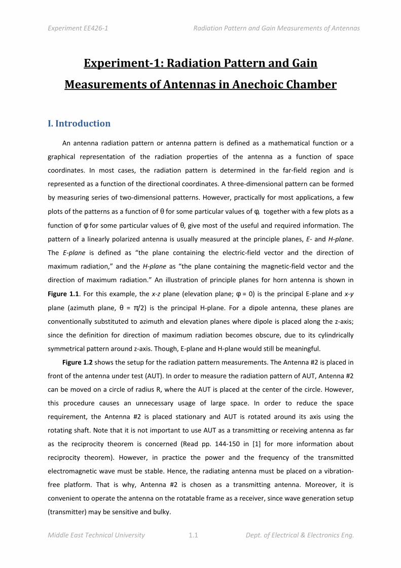
direction of maximum radiation.” An illustration of principle planes for horn antenna is shown in
Figure 1.1. For this example, the x-z plane (elevation plane; φ = 0) is the principal E-plane and x-y
plane (azimuth plane, θ = π/2) is the principal H-plane. For a dipole antenna, these planes are
conventionally substituted to azimuth and elevation planes where dipole is placed along the z-axis;
since the definition for direction of maximum radiation becomes obscure, due to its cylindrically
symmetrical pattern around z-axis. Though, E-plane and H-plane would still be meaningful.
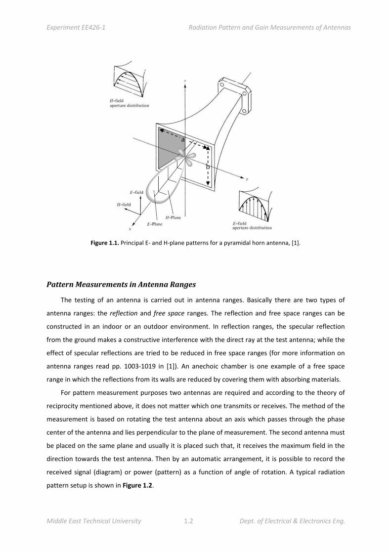
Figure 1.2 shows the setup for the radiation pattern measurements. The Antenna #2 is placed in
front of the antenna under test (AUT). In order to measure the radiation pattern of AUT, Antenna #2
can be moved on a circle of radius R, where the AUT is placed at the center of the circle. However,
this procedure causes an unnecessary usage of large space. In order to reduce the space
requirement, the Antenna #2 is placed stationary and AUT is rotated around its axis using the
rotating shaft. Note that it is not important to use AUT as a transmitting or receiving antenna as far
as the reciprocity theorem is concerned (Read pp. 144-150 in [1] for more information about
reciprocity theorem). However, in practice the power and the frequency of the transmitted
electromagnetic wave must be stable. Hence, the radiating antenna must be placed on a vibration-
free platform. That is why, Antenna #2 is chosen as a transmitting antenna. Moreover, it is
convenient to operate the antenna on the rotatable frame as a receiver, since wave generation setup
(transmitter) may be sensitive and bulky.
Experiment EE426-1 Radiation Pattern and Gain Measurements of Antennas
Middle East Technical University 1.2 Dept. of Electrical & Electronics Eng.
a
b
Figure 1.1. Principal E- and H-plane patterns for a pyramidal horn antenna, [1].
Pattern Measurements in Antenna Ranges
The testing of an antenna is carried out in antenna ranges. Basically there are two types of
antenna ranges: the reflection and free space ranges. The reflection and free space ranges can be
constructed in an indoor or an outdoor environment. In reflection ranges, the specular reflection
from the ground makes a constructive interference with the direct ray at the test antenna; while the
effect of specular reflections are tried to be reduced in free space ranges (for more information on
antenna ranges read pp. 1003-1019 in [1]). An anechoic chamber is one example of a free space
range in which the reflections from its walls are reduced by covering them with absorbing materials.
For pattern measurement purposes two antennas are required and according to the theory of
reciprocity mentioned above, it does not matter which one transmits or receives. The method of the
measurement is based on rotating the test antenna about an axis which passes through the phase
center of the antenna and lies perpendicular to the plane of measurement. The second antenna must
be placed on the same plane and usually it is placed such that, it receives the maximum field in the
direction towards the test antenna. Then by an automatic arrangement, it is possible to record the
received signal (diagram) or power (pattern) as a function of angle of rotation. A typical radiation
pattern setup is shown in Figure 1.2.
Experiment EE426-1 Radiation Pattern and Gain Measurements of Antennas
Middle East Technical University 1.3 Dept. of Electrical & Electronics Eng.
II. Preliminary Work
1. Read the sections related to radiation pattern measurements and polarization pattern
measurements in [1] (pp. 1021-1028 and 1038-1043 respectively).
2. Read the sections related to gain measurements in [1] (pp. 1028-1034).
3. Derive the formula for measuring the gain of an antenna by means of a standard-gain antenna
whose gain is characterized and known.
Hint: Use the Friis transmission equation:
=
4 (1)
where Pt and Pr the transmitted and received powers at the transmitting and receiving antennas,
respectively. Gt and Gr are the transmitting and receiving antenna gains. λ is the free space
wavelength and R is the distance between the antennas.
III. Experimental Procedure
The measurements will be performed under the guidance of the assistant.
1. Initiate the setup in Figure 1.2.
Transmitting Antenna
Receiving Antenna
To Computer
To Receiver
To Generator
Rotating shaft
AUT R Antenna2
Figure 1.2. Setup for the radiation pattern measurements.

Experiment EE426-1 Radiation Pattern and Gain Measurements of Antennas
Middle East Technical University 1.4 Dept. of Electrical & Electronics Eng.
2. Measure the radiation pattern of the following antennas at 9 GHz for E- and H-planes. In
addition, determine and record the maximum power received, note the polarizations, and define
the HPBW (half-power beamwidth):
a. Standard-gain horn (pyramidal horn with dimensions a=b=7.5 cm),
b. Pyramidal horn (a= 17.8 cm, b=15.4 cm),
c. E-plane sectoral horn (a= 2.3 cm, b= 10 cm).
Fill in the table below with your observations.
Antenna HPBW
(E-plane)
HPBW
(H-plane)
Max. Received
Power (dBm)
Gain
(dB)
Type of
Polarization
Standard Gain Horn
Pyramidal Horn
E-plane Sectoral Horn
3. Measure the cross pol. pattern of the standard-gain horn.
4. Measure the gain of the pyramidal horn (a= 17.8 cm, b=15.4 cm) at 9 GHz using the standard-
gain horn (a pyramidal horn antenna with dimensions a=b=7.5 cm).
5. Measure the gain of the E-plane sectoral horn (a= 2.3 cm, b= 10 cm) at 9 GHz using the standard-
gain horn.
NOTICE:
The patterns will be sent via e-mail by the assistants.
IV. Results and Comments
1. For each of the antennas measured,
a. Plot the E- and H-plane radiation patterns and indicate the polarization of the antenna
(linear, circular or elliptical).
Note: The values of the radiation pattern data are in dB scale. Plot the normalized
radiation patterns in rectangular coordinates.
b. Calculate and tabulate the half-power beamwidths (HPBW) both obtained from the
pattern data that have been sent by email and the ones that you have recorded during
the experimental procedure. Comment on the discrepancies between the HPBW values
Experiment EE426-1 Radiation Pattern and Gain Measurements of Antennas
Middle East Technical University 1.5 Dept. of Electrical & Electronics Eng.
that you have recorded and the ones obtained from the radiation pattern graphs. Also,
include the first null beamwidth (FNBW) values in both planes in your tabulation.
c. Compare and tabulate the directivity values obtained using Krauss' formula with the gain
values measured in the experiment. Explain the discrepancies between them.
2. Plot the normalized co-pol. pattern of standard horn in rectangular coordinates. Then plot the
cross-pol. radiation pattern of standard horn antenna on the same graph and comment.
Note: The values of the radiation pattern data are in dB scale. Note that the cross-pol. pattern
should be normalized with respect to the maximum of the co-pol. pattern.
3. Compare the antennas with each other in terms of their gains, HPBWs and FNBWs considering
their relative dimensions.
4. Write your overall comments about this experiment. Specifically, comment on the experimental
setup and summarize the main principles you learned in a few sentences.
V. References
[1] C. A. Balanis, Antenna Theory, Analysis and Design, 3rd Edition, John Wiley & Sons, NY, 2005.
[2] J. D. Kraus, Antennas, McGraw Hill, New York, 1988.

Experiment EE426-2 Radiation Pattern Measurements of Antennas
Middle East Technical University 2.1 Dept. of Electrical & Electronics Eng.
Experiment-2:RadiationPatternMeasurementsof
Antennas
I.Introduction
Two of the most important characteristics of an antenna are its directional diagram (or radiation
pattern) and its polarization pattern. The purpose of this experiment is to measure the radiation
pattern of wire-type antennas (also known as linear antennas) and printed patch antennas. We will
investigate the polarization characteristics and bandwidths of these antennas in Experiment-3.
For more information on radiation pattern measurements, refer to the Introduction section of
Experiment-1.
Near and Far-Field Properties
The space around an antenna is usually divided into three regions: (a) reactive near-field,
(b) radiating near-field (Fresnel), and (c) far-field (Fraunhofer) regions. These regions are designated
according to the general form of their electromagnetic fields.
Far-field region is defined as the region of an antenna where the angular field distribution is
essentially independent of the observation range. In other words, electric (or magnetic) fields have
the general expression =
(, ), where (, φ) is the angular field distribution and it does
not depend on range. In this region, the radial field component is negligible and the field components
are essentially transverse to radial (propagation) direction, thereby forming a spherical TEM wave.
A Brief Summary of the Antenna Types used in the Experiment
⁄ dipole: The half-wave dipole is one of the most commonly used antennas. Besides their simple
construction, another reason for its popularity is that its input impedance (for very thin dipoles)
= 73 + 42.5Ω
is very close to the 50Ω or 75Ω characteristic impedance of most transmission lines, which simplifies
its matching especially at resonance. In general, the input impedance of a dipole is a function of its
length: For the special choice of half-wavelength, the input resistance becomes equal to the radiation
resistance, and input reactance becomes slightly inductive (hence the half-wave dipole is not

Experiment EE426-2 Radiation Pattern Measurements of Antennas
Middle East Technical University 2.2 Dept. of Electrical & Electronics Eng.
resonant). The dipole reactance also depends on the dipole arm thickness as well as the gap between
those arms.
In order to perform a good impedance match to a transmission line, one must eliminate the
input reactance of the dipole. This can be done with an external matching network employed behind
the dipole. A more practical and popular means to cancel the half-wave dipole reactance (hence to
make it resonant) is to slightly trim its arm length (which makes it less inductive according to the
transmission line theory) [2].
Folded Dipole: Dipole antennas can be placed in parallel to produce more radiation: When dipoles
are in close proximity, they can create a radiated power that is greater than that of a single
dipole, where is the number of dipoles. Figure 2.1 illustrates a folded dipole for = 2, ! = " 2⁄ ,
# ≪ ", % ≪ ". The antenna is fed at the center of one dipole, which is a key point in feeding. At low
frequencies (when the antenna is electrically small), the current induced on the two arms tends to
cancel each other, and the antenna does not radiate well. At higher frequencies (particularly when
the arms are λ/2-long), however, the induced currents become in phase to reinforce their radiation.
Hence at resonance, this structure acts like two closely-spaced dipoles which double the radiated
field (and quadruple the radiated power). The folded dipole has a similar radiation pattern to that of
a standard dipole; but it radiates more efficiently with a radiation resistance of &'( = &()*+ =
73,2 ≅ 300Ω [3].
Figure 2.1. Folded dipole, [1].
Yagi-Uda Antenna: A Yagi-Uda antenna consists of a number of linear dipole elements. One of its
dipole elements is energized directly by a feed transmission line, while the others act as parasitic
radiators whose currents are induced by mutual coupling. The antenna is exclusively designed to
operate as an end-fire array, and this is accomplished by having the parasitic elements in the forward
direction act as directors while those in the rear act as reflectors.
Experiment EE426-2 Radiation Pattern Measurements of Antennas
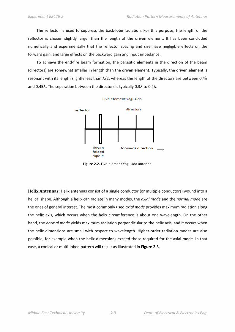
Middle East Technical University 2.3 Dept. of Electrical & Electronics Eng.
The reflector is used to suppress the back-lobe radiation. For this purpose, the length of the
reflector is chosen slightly larger than the length of the driven element. It has been concluded
numerically and experimentally that the reflector spacing and size have negligible effects on the
forward gain, and large effects on the backward gain and input impedance.
To achieve the end-fire beam formation, the parasitic elements in the direction of the beam
(directors) are somewhat smaller in length than the driven element. Typically, the driven element is
resonant with its length slightly less than λ/2, whereas the length of the directors are between 0.4λ
and 0.45λ. The separation between the directors is typically 0.3λ to 0.4λ.
Figure 2.2. Five-element Yagi-Uda antenna.
Helix Antennas: Helix antennas consist of a single conductor (or multiple conductors) wound into a
helical shape. Although a helix can radiate in many modes, the axial mode and the normal mode are
the ones of general interest. The most commonly used axial mode provides maximum radiation along
the helix axis, which occurs when the helix circumference is about one wavelength. On the other
hand, the normal mode yields maximum radiation perpendicular to the helix axis, and it occurs when
the helix dimensions are small with respect to wavelength. Higher-order radiation modes are also
possible, for example when the helix dimensions exceed those required for the axial mode. In that
case, a conical or multi-lobed pattern will result as illustrated in Figure 2.3.

Experiment EE426-2 Radiation Pattern Measurements of Antennas
Middle East Technical University 2.4 Dept. of Electrical & Electronics Eng.
Figure 2.3. Helix geometry and three radiation modes [2].
Microstrip Patch Antennas: Microstrip patch antennas are popular among the antenna
community because they are low-profile, conformable to planar or nonplanar surfaces, mechanically
robust when mounted on a rigid body, and are simple and inexpensive to manufacture using modern
printed circuit technology. The microstrip patch antenna comprises a metallic patch of a given shape
(rectangular, circular, oval, etc.) placed on a thin dielectric substrate, and is backed by a ground
plane. This antenna is designed to have its pattern maximum normal to the patch, which is
accomplished by properly choosing the mode (field configuration under the patch). A rectangular
microstrip patch antenna, which we will use in the experiment, can be represented as an array of two
radiating narrow apertures (slots) constructed by the fringing fields (see Figure 2.4) [1].
Figure 2.4. Microstrip antenna [1].

Experiment EE426-2 Radiation Pattern Measurements of Antennas
Middle East Technical University 2.5 Dept. of Electrical & Electronics Eng.
λ/2 dipole Folded dipole Circularly polarized
patch
Linearly polarized
patch
3-element Yagi-Uda 5-element Yagi-Uda Helix antenna
Figure 2.5. Antennas that will be characterized in the experiment.
II. Preliminary Work
1. Read the section related to radiation pattern measurements in [1] (pp. 1021-1028).
2. Define the E- and H-planes of an antenna and show them for wire-type antennas. Can we define
E- and H-planes for circularly polarized antennas? Why?
3. For the antennas given below, plot the radiation patterns in E- and H-planes on the same graph,
determine the half power beamwidths (HPBW) and the first null beamwidths (FNBW).
a. λ/2 dipole antenna
b. λ/4 monopole on an infinite ground plane
4. Roughly plot the radiation patterns of the following antennas on the same graph, [1]:
a. Microstrip rectangular patch antenna
b. Yagi-Uda antenna
5. Make a comparison between a Yagi-Uda antenna and a simple λ/2 dipole in terms of beamwidth,
directivity, and back-lobe radiation.
6. Calculate the Rayleigh distance of the λ/2 dipole at 8.5 GHz, 9.0 GHz, 9.5 GHz. How does the
magnitude of the field change with the distance from the antenna up to and beyond the Rayleigh
distance?
REMARK:
Keep a copy of your preliminary work in order to compare the theoretical results you obtained
with measured ones in your report.

Experiment EE426-2 Radiation Pattern Measurements of Antennas
Middle East Technical University 2.6 Dept. of Electrical & Electronics Eng.
III. Experimental Procedure
1. Initiate the computer controlled system (Lucas-Nülle antenna measurement setup) shown in
Figure 2.6 under the guidance of your assistants.
NOTE:
• During the measurements, the height of the antennas must be adjusted for proper vertical
alignment with respect to their centers.
• Make sure that the receiving and transmitting antennas are aligned in polarization
before conducting your measurements.
• Save your data in a file at each step. At the end of the experiment, remove your data files
from the hard disk of the computer after copying them onto a memory stick.
Figure 2.6. Setup for the radiation pattern measurements.
2. Measure and plot the axial amplitude variation of the field of a λ/2 dipole antenna at the
operating frequency (DRO frequency of the measurement system). To do this, first set the

Experiment EE426-2 Radiation Pattern Measurements of Antennas
Middle East Technical University 2.7 Dept. of Electrical & Electronics Eng.
spacing between the receiver and transmitter platforms to 20 cm. Measure and record the
received power. Increase the distance between the antennas in 10 cm steps up to 100 cm, and
record the received power at each step. Fill in Table 1 for your reference.
Table 1. Amplitude variation of the λ/2-dipole field measured in step 2.
fop=……..GHz Distance (cm) 20 30 40 50 60 70 80 90 100
Power Level (dBm)
3. Measure the radiation patterns in both E- and H-planes of the following antennas at the
corresponding DRO frequency. For each measurement, first observe the pattern in polar form
and save this polar plot to your folder. Then switch to the rectangular coordinates (in dB scale),
find the HPBW and FNBW in degrees using data cursors, and save this rectangular graph to your
folder (with the cursors clearly showing the HPBW value). In addition, fill in Table 2 for your
reference.
a. λ/2 dipole antenna
b. Monopole
c. Folded dipole
d. 3-element and 5-element Yagi-Uda antennas
e. RHCP rectangular patch antenna
f. Linearly polarized patch antenna
Table 2. Pattern data for the antennas in step 3.
Antenna Types HPBW(E-plane) FNBW(E-plane) HPBW(H-plane) FNBW(H-plane)
λ/2 dipole antenna
Monopole
Folded dipole
3-element Yagi-Uda
5-element Yagi-Uda
RHCP patch antenna
LP patch antenna

Experiment EE426-2 Radiation Pattern Measurements of Antennas
Middle East Technical University 2.8 Dept. of Electrical & Electronics Eng.
IV. Results and Comments
1. Plot the axial amplitude distribution of the λ/2-dipole antenna in step 2. Do not forget to convert
your measurements to linear scale. Compare this result with your answer to part 6 of the
preliminary work. Validate your measurement by fitting your measured data to an appropriate
function of the range.
2. For each antenna measured in the experiment,
a. Plot the E- and H-plane radiation patterns, and compare them with the ones obtained in
your preliminary work.
b. Determine and tabulate the HPBW and FNBW of each antenna. Compare the measured
HPBW and FNBW of the λ/2-dipole with the ones obtained in your preliminary work.
V. References
[1] C. A. Balanis, Antenna Theory, Analysis and Design, 3rd Edition, John Wiley & Sons, NY, 2005.
[2] J. L. Volakis, Antenna Engineering Handbook, 4th ed. New York: McGraw-Hill, 2007.
[3] R. Schmitt, A Handbook for wireless/RF,EMC, and High-Speed Electronics, Elsevier Sci., 2002.

Experiment EE426-3 Polarization Pattern and Bandwidth Measurements
Middle East Technical University 3.1 Dept. of Electrical & Electronics Eng.
Experiment-3:PolarizationPatternandBandwidth
MeasurementsofAntennas
I.Introduction
In this experiment, we will investigate the polarization pattern and bandwidth of the antennas
which were previously introduced in Experiment-2.
Polarization of an Antenna
Polarization of an antenna reflects the vector nature of its radiation pattern, and it is
conventionally defined through the polarization of the electromagnetic wave radiated from that
antenna (in transmit mode) at a given far-field observation point [1]. As may be remembered from
your earlier electromagnetic courses, the electric field vector of an electromagnetic wave traces a
path over time at a certain point in space, and this path defines the polarization of that wave. In
general, the mentioned path turns out to be an ellipse (elliptical polarization); but it is possible to
obtain a line or a circle under some special cases (leading to linear and circular polarizations,
respectively). Let us refresh our memory of these polarization types:
LinearPolarization: A time-harmonic wave is linearly polarized at a given point in space, if the
electric field vector at that point is always oriented along the same straight line at all times. This is
accomplished if the field vector possesses
a. Only one component, or
b. Two orthogonal components that are in- or out-of-phase (i.e., the phase difference between
these orthogonal components is , ∈ ℤ).
CircularPolarization: A time-harmonic wave is circularly polarized at a given point in space if the
electric field vector at that point traces a circle as a function of time. The circularly polarized wave
satisfies each of the following conditions:
a. The field must have two orthogonal components, and
b. These two field components must have the same magnitude, and
c. These two field components must have a phase difference of ()
, ∈ ℤ (i.e., they must
be in phase-quadrature).

Experiment EE426-3 Polarization Pattern and Bandwidth Measurements
Middle East Technical University 3.2 Dept. of Electrical & Electronics Eng.
If the fingers of the right hand follow the direction of the rotation of E-field vector and the
thumb points to the direction of propagation of the wave, then the wave is right hand circularly
polarized (RHCP). Conversely, the wave is left hand circularly polarized (LHCP) if you satisfy this
orientation with your left hand.
Elliptical Polarization: A time-harmonic wave is elliptically polarized if the electric field vector
traces an elliptical locus in space as a function of time. Although linear and circular polarizations are
special cases of elliptical polarization, in practice we reserve the term elliptical polarization to waves
which are not linearly or circularly polarized. The necessary and sufficient conditions for elliptically
polarized wave are as follows:
a. The field must have two orthogonal components, and
b. These two components can be of the same or different magnitude.
c. (i) If the two field components are not of the same magnitude, they can differ in phase by an
arbitrary amount (except for , since otherwise the wave becomes linearly polarized).
(ii) If the two components are of the same magnitude, they can differ in phase by an
arbitrary amount (except for
, since otherwise the wave becomes linearly or circularly
polarized).
If the fingers of the right hand follow the direction of the rotation of E-field vector and the
thumb points to the direction of propagation of the wave, then the wave is right hand elliptically
polarized (RHEP). Conversely, the wave is left hand elliptically polarized (LHEP) if you satisfy this
orientation with your left hand.
Polarization Pattern Measurements
For the polarization pattern measurements, two antennas are positioned as shown in Figure 2.7
so that their maximum radiation axes coincide with the rotation axis. The transmitting antenna is
linearly polarized. The test antenna is rotated in the plane of polarization and its received signal is
recorded. A plot of the received signal level as a function of rotation angle yields the polarization
pattern, from which polarization type and the ellipticity ratio can easily be inferred. Note that the
roles of the transmitting and receiving antennas can be interchanged in this setup owing to the
reciprocity theorem.

Experiment EE426-3 Polarization Pattern and Bandwidth Measurements
Middle East Technical University 3.3 Dept. of Electrical & Electronics Eng.
Bandwidth of an Antenna
IEEE defines the bandwidth as "the range of frequencies within which the performance of the
antenna, with respect to some characteristic, conforms to a specified standard." Conventionally,
mentioned “characteristics” may be the return loss level, polarization, radiation pattern constraints.
The operating band of the antenna can be defined as the frequency band around the resonance
frequency within which the return loss is less than a desired ratio, say 10 dB. Thus the 10 dB return
loss bandwidth corresponds to the frequency band over which at least nine tenth of the power is
transmitted to the antenna.
II. Preliminary Work
1. Read the section related to polarization pattern measurements in [1] (pp. 1038-1043).
2. Draw the polarization patterns for three types of polarizations. Define geometrically the
ellipticity ratio for each type of polarization.
3. Indicate the polarizations the following antennas:
a. λ/2 dipole antenna, b. λ/4 monopole antenna, c. helix antenna,
d. Yagi-Uda antenna, e. Microstrip rectangular patch.
4. Consider the return loss of a dipole antenna shown in Figure 3.1. For this antenna find:
a. 10 dB and 15 dB bandwidths.
b. VSWR 3:1 bandwidth.
8 8.5 9 9.5 10 10.5 11 11.5 12-35
-30
-25
-20
-15
-10
-5
0
S 11
(dB
)
Frequency (GHz) Figure 3.1. Return loss of a dipole antenna.

Experiment EE426-3 Polarization Pattern and Bandwidth Measurements
Middle East Technical University 3.4 Dept. of Electrical & Electronics Eng.
III. Experimental Procedure
1. Initialize the Lucas-Nülle antenna measurement setup that you have used in Experiment-2. In
order to measure the polarization pattern of antennas, make the necessary changes to obtain
the setup shown in Figure 3.2.
Receiving Antenna (AUT)
Transmitting Antenna
Figure 3.2. Setup for polarization pattern measurements.
NOTE:
• Prior to the measurements, the receiving and transmitting antennas must be properly
aligned to have their antenna centers lying on the rotation axis.
• Save your data in a file at each step. At the end of the experiment, remove your data files
from the hard disk of the computer after copying them onto a memory stick.

Experiment EE426-3 Polarization Pattern and Bandwidth Measurements
Middle East Technical University 3.5 Dept. of Electrical & Electronics Eng.
2. Obtain the polarization patterns of the following antennas. Do not forget to save your pattern for
each antenna in polar coordinates (in dB scale).
a. λ/2 dipole antenna,
b. Linearly polarized patch antenna,
c. Circularly polarized patch antennas (both LHCP and RHCP ones),
d. RHCP helix antenna (measure the polarization pattern along and off the helix axis).
NOTE:
In order to continue with the following steps, first perform a calibration over 6.0-12.5 GHz
frequency interval using the instructions described in section VI (“Network Analyzer 1-Port
Calibration Instructions”) found in the introduction part of the manual.
3. Measure the return loss of the following antennas using Agilent E5071C Network Analyzer over
6.0-12.5 GHz frequency band, and analyze their frequency responses. After inspecting the
measured reflection coefficient, store it by pressing Save/RecallSnPS1P (make sure to assign
a distinct filename for each antenna). You will later use these files to determine the 10 dB/15 dB
bandwidths, the input impedance at the operating frequency, and the input impedance at the
frequency where the best match is achieved for each antenna type (see Table 1).
a. λ/2 dipole antenna,
b. Monopole antenna,
c. RHCP helix antenna,
d. Five-element Yagi-Uda antenna,
e. LP microstrip rectangular patch antenna.
Table 1. Measured bandwidths and impedances of the antennas in step 3.
Antenna Types Input impedance
at fop=……GHz
Input impedance value
for best match case (MHz) (MHz)
λ/2 dipole antenna …...……… Ω @ ……GHz ……dB BW: .…..dB BW:
monopole antenna …...……… Ω @ ……GHz ……dB BW: …...dB BW:
RHCP helix antenna …...……… Ω @ ……GHz ……dB BW: .…..dB BW:
5-element Yagi-Uda …...……… Ω @ ……GHz ……dB BW: .…..dB BW:
LP microstrip patch …...……… Ω @ ……GHz …...dB BW: .…..dB BW:
4. Measure the return loss of the printed spiral antenna in 100 MHz-14 GHz band, and store its data
in an S1P file. Using this file, you will later determine the 10 /15 dB bandwidths of this antenna.

Experiment EE426-3 Polarization Pattern and Bandwidth Measurements
Middle East Technical University 3.6 Dept. of Electrical & Electronics Eng.
IV. Results and Comments
1. Plot the polarization patterns of the antennas measured in step 2. Determine and tabulate their
ellipticity ratios, types and senses of polarizations. Show your calculation in detail.
2. For each antenna characterized in step 3, plot the measured return loss as a function of
frequency and draw the corresponding impedance pattern on a Smith Chart. Calculate the
bandwidth of each antenna, and determine the impedance at the operating frequency. Comment
on the bandwidths of the antennas. Do not forget to include your results in Table 1.
3. Comment on whether the antennas are properly designed or not by comparing the input
impedance values at the operating frequency and at the best-match frequency. Compare the
bandwidth of the spiral antenna with the bandwidths of the wire and patch antennas.
4. Write your overall comments about this experiment.
INFORMATION:
For return loss and Smith Chart plotting tasks, you may use the MATLAB routines provided on
METU-Online. You will also find a sample script utilizing those routines to get you started.
V. References
[1] C. A. Balanis, Antenna Theory, Analysis and Design, 3rd Edition, John Wiley & Sons, NY, 2005.
[2] J. L. Volakis, Antenna Engineering Handbook, 4th ed. New York: McGraw-Hill, 2007.
[3] R. Schmitt, A Handbook for wireless/RF,EMC, and High-Speed Electronics, Elsevier Sci., 2002.

Experiment EE426-4 Linear Antennas: Impedance & Pattern Measurements
Middle East Technical University 4.1 Dept. of Electrical & Electronics Eng.
Experiment-4:LinearAntennas:Impedance&Pattern
Measurements
I.Introduction
This experiment aims to investigate wire-type antennas in terms of their radiation pattern, input
impedance, bandwidth, and current/voltage distribution. The effects of a nearby ground plane on
these characteristics will also be studied. In particular, the following items will be covered:
• Radiation patterns of wire antennas (dipole, monopole antennas and log-periodic dipole
arrays) will be measured at various frequencies, and these patterns will be interpreted in
terms of electrical length.
• Ground plane effects will be investigated through measurements of a horizontal half-wave
dipole and a vertical monopole placed above a conducting plane (which simulates the earth).
• Current and voltage distributions on dipoles of different electrical length will be measured
with near-field probes.
• Input impedance and impedance bandwidth of wire antennas will be studied.
λ/2 Dipole: The input impedance of an infinitely thin, perfectly conducting, half-wave dipole
antenna is = 73.1 + 42.3Ω. This is a good approximation for a half-wave dipole constructed
from a wire of diameter 2 which is much smaller than its length 2ℓ (i.e., ≪ ℓ). To tune the
antenna, the half length must be shortened approximately by
Δℓ
ℓ =0.225 ℓ2
(1)
where ℓ = /4. A tuned dipole has a resistive input impedance about 70 Ω, and it is called the
resonant dipole. Voltage and current distributions on the half-wave dipole are shown in Figure 4.1.
Figure 4.1. Voltage and current distributions on a resonant dipole.
I I
I V
ℓ − Δℓ

Experiment EE426-4 Linear Antennas: Impedance & Pattern Measurements
Middle East Technical University 4.2 Dept. of Electrical & Electronics Eng.
For matching purposes, the characteristic impedance of the transmission line connected to the
feeding points must be equal to the input impedance of the antenna. Under matched conditions, the
maximum power will be radiated from the antenna. The efficiency of this antenna, like any other
wire-type one, is determined by the loss resistance of the wire. The loss resistance is usually
negligible at low frequencies, and it increases with the frequency because of the skin effect.
The reactance of the antenna is capacitive below the resonance frequency, and it becomes
inductive for operation above the resonance frequency. One may understand this input impedance
behavior as well as the current/voltage distribution trends by envisioning the half-wave dipole as an
open-circuited quarter-wave transmission line.
The radiation pattern of a half-wave dipole antenna is similar to that of a short dipole: It is a
“circle” in the azimuth plane (φ-plane) and a “figure-of-eight” in the elevation plane (θ-plane) of the
antenna.
When the half-wave dipole antenna is placed over a conducting plane (e.g., earth), its input
impedance deviates from the nominal 73.1 + 42.3Ω value. For a horizontal half-wave dipole above
a perfectly conducting plane, the input impedance increases with height from zero to a very high
value (with a resistive component of approximately 95 Ω), and the impedance oscillates about its
free-space value as the height increases further [1].
Balun: Balun structures are used at the feed of dipole antennas. The word “balun” is an
abbreviation for “balanced-to-unbalanced transformation”. A coaxial cable is an unbalanced
transmission line, because the inner and the outer conductors of coaxial cable are not interfaced to
the antenna in the same way. This is illustrated in Figure 4.2 (a): Unlike the inner conductor, the
outer coaxial conductor may carry current on both of its inside and outside surfaces. Due to these
multiple current paths, a nonzero current (spill-over current, ) flows to the ground on the outside
surface of the outer conductor, an outcome which disturbs the balance of the dipole arm currents (
versus − ).
Baluns can be used to balance inherently unbalanced systems, by canceling the spill-over
current (). The type of balun used in the experiment is shown in Figure 4.2 (b). It requires that one
end of a λ/4-section of an auxiliary coaxial line be connected to the outside shield of the main coaxial
line (node B), while the other end is connected to the dipole arm which is attached to the center
conductor (node C). The voltages at nodes A and C are nearly equal in magnitude (but are out-of-
phase), and the shield construction of both coaxial cables is identical so that their impedances to the
ground are similar. Accordingly, a net current of flows toward the node C which balances the
currents on the dipole arms ( − ) as shown in Figure 4.2 (b). One would also like to set = 0 for

Experiment EE426-4 Linear Antennas: Impedance & Pattern Measurements
Middle East Technical University 4.3 Dept. of Electrical & Electronics Eng.
proper dipole radiation characteristics: When the length of the auxiliary transmission line is λ/4,
will be zero so that the dipole arms will carry equal currents of .
(a) Unbalanced coaxial line (b) λ/4 coaxial balun
Figure 4.2. Unbalanced coaxial line and the quarter-wave balun.
Vertical Monopole: A vertical monopole antenna is an asymmetrical dipole antenna as shown in
Figure 4.3. According to the image theory, the effect of earth can be accounted for by considering a
symmetrical dipole which radiates only in upper half-space. Thus !! = "#!$%/2. The monopole
antenna can be directly fed by a coaxial cable, and it does not require a balun. The radiation pattern
is the same as that of dipole antenna in the upper half-space and zero in the lower half-space.
Figure 4.3. Vertical monopole antenna.
Log-Periodic Dipole Array: An array with a gradually expanding periodic structure has electrical
properties which also vary periodically in a manner depending on its structure. The geometry of the
antenna is chosen so that electrical properties repeat periodically with the logarithm of the
frequency. Log-periodic dipole array consists of a sequence of side-by-side parallel linear dipoles, as
shown in Figure 4.4.
I1 I2
I1-I2
I1
Antenna
I1
z
x
λ/4
Image
Antenna I1-I2 I1-I2 I1
A
λ/4 I2
I1 I1
I2
B
Shorted together
C

Experiment EE426-4 Linear Antennas: Impedance & Pattern Measurements
Middle East Technical University 4.4 Dept. of Electrical & Electronics Eng.
Figure 4.4. Log-periodic dipole array.
There are certain similarities between the log-periodic array and the Yagi-Uda array; however,
the log-periodic array operates in a much wider bandwidth. Unlike the Yagi-Uda array whose
geometric dimensions do not follow any pattern; the lengths (ℓ), spacings (&), diameters (') and
even gap spacing at dipole centers of the log-periodic array increase logarithmically as defined by the
inverse of geometric ratio τ:
ℓ(ℓ= &(&
= '('= 1)
(2)
Another parameter associated with log periodic array is spacing factor σ, and it is defined as
* &( &
2ℓ(
1 )
4 tan. (3)
By using these parameters, directivity of the log-periodic array can be found from the contours
provided in Figure 4.5. E-plane beamwidth is determined mostly by the dipole pattern and is
approximately 60°, whereas the H-plane beamwidth may be determined from the Kraus’ formula:
/ 41253
012 3 014
(3)
In (3), / stands for the directivity, and 012 and 014 represent the half power beamwidths (HPBW,
in degrees) in E- and H-planes respectively.
Input Impedance Measurements and Bandwidth of an Antenna
The reflection coefficient (Γ) is the ratio of the reflected wave phasor to the incident one at the
specified terminals. The input reflection coefficient Γ6ℓ, as shown in Figure 4.6, is easily formulated
using the feed line characteristic impedance (7) and the load (antenna) impedance (8). The
derivations are given below, refer to [2] for more information.

Experiment EE426-4 Linear Antennas: Impedance & Pattern Measurements
Middle East Technical University 4.5 Dept. of Electrical & Electronics Eng.
Figure 4.5. Computed contours of constant directivity versus σ and τ for log-periodic dipole arrays [1].
Figure 4.6. Parameter definitions for reflection coefficient calculations.
8999 =87 , Γ60 = 8
999 − 18999 1
|Γ6ℓ| <=1&6ℓ 1
<=1&6ℓ 1
Γ6ℓ Γ60>?@ℓ, A . B
For a lossless line: Γ6ℓ Γ60>?CDℓ
Return loss: RL 20 log76|Γ6ℓ|
Since the electrical length of the transmission line (J Bℓ) is a linear function of frequency and
the load might exhibit a nontrivial frequency response (i.e., 8 86K), the reflection coefficient Γ
varies with frequency in general. Variation of Γ with frequency translates to a similar variation in the
power being delivered to the load (∝ 1 |Γ|). This is especially true for narrowband networks, for
ℓ
Γ6ℓ
8 7, A
Γ8 Γ60

Experiment EE426-4 Linear Antennas: Impedance & Pattern Measurements
Middle East Technical University 4.6 Dept. of Electrical & Electronics Eng.
which a slight deviation from the matched operation frequency causes an appreciable drop in the
delivered power. In practice, it is difficult to realize perfect matching at a given operating frequency
due to losses, impedance variations and fabrication tolerances; that is the reason why engineers
define an acceptable reflection level and an associated bandwidth.
IEEE defines the bandwidth as "the range of frequencies within which the performance of the
antenna, with respect to some characteristic, conforms to a specified standard." Conventionally,
mentioned “characteristics” may be the return loss level, polarization, radiation pattern constraints.
The operating band of the antenna can be defined as the frequency band around the resonance
frequency within which the return loss is less than a desired ratio, say 10 dB. Thus the 10 dB return
loss bandwidth corresponds to the frequency band over which at least nine tenth of the power is
transmitted to the antenna.
In order to measure the input impedance of an antenna and its return loss bandwidth, a vector
network analyzer (VNA) is employed in the laboratory. This is an instrument which measures the
scattering parameters (S-parameters) of LTI microwave networks. When used for one-port
measurements, the measurement result corresponds to the reflection coefficient (also represented
with =). The instrument can also display the impedance of the tested network on a Smith Chart
over a frequency range. Prior to the measurements, the network analyzer is calibrated to shift the
reference planes to the ends of its test port cables.
Measurement of Current and Voltage (Amplitude) Distributions
The current (voltage) distribution on an antenna can be sampled by using magnetic (electric)
field probes. For current measurements, a small loop (Figure 4.7.a) is brought close to the antenna
conductor and the current induced in the loop is measured. According to the Faraday’s law, the
induced emf over the loop is proportional to the captured flux at the sampling position, which is in
turn proportional to the antenna current at that location. Consequently, the antenna current
distribution can be determined by monitoring the current induced on the loop (which is related to
the induced emf through the loop’s resistance) at several sampling positions.
Similarly, voltage distribution measurements can be made by using a small voltage sampling
probe. A small dipole or monopole (Figure 4.7.b) can be used for this purpose. The electric field of
the antenna (along the direction of the probe) induces a current on the dipole or monopole, and this
induced current is approximately proportional to the antenna voltage at that particular sampling
position.
In order to avoid disturbing the near-field of the test antenna (hence its current and voltage
distributions), the current/voltage sampling probes must be small with respect to the wavelength.

Experiment EE426-4 Linear Antennas: Impedance & Pattern Measurements
Middle East Technical University 4.7 Dept. of Electrical & Electronics Eng.
During the experiment, we will use a small loop antenna and a small monopole as illustrated in
Figure 4.7.
(a) (b)
Figure 4.7. (a) Shielded current sampling loop (magnetic field probe), (b) voltage sampling monopole (electric
field probe).
II. Preliminary Work
1. Read the sections related to the impedance measurements (pp. 1036-1038) and current
measurements (pp. 1038) in [1].
2. Indicate the polarization of a dipole antenna. For the antennas described below, draw the
radiation patterns in E- and H-planes, and determine the half-power and first-null beamwidths
(HPBW, FNBW) at each provided frequency:
a. λ/2 dipole antenna of 8.4 cm length at the resonance frequency,
b. 8.4 cm-long dipole antenna at 1.2 GHz, 1.5 GHz, 1.8 GHz,
c. 35 cm-long dipole antenna at 1.285 GHz and 1.714 GHz.
You may check your patterns with the dipole patterns provided in [1] for different electrical
lengths.
3. Calculate the resonant length of a half-wave dipole antenna made from a round copper wire of
radius = 0.3MN and operating at a frequency of 1 GHz.
4. Plot the input resistance as a function of the height (O) for the horizontal half-wave dipole in
Figure 4.8. What is the input resistance at O λ/2? Hint: See pp. 204 in [1]).

Experiment EE426-4 Linear Antennas: Impedance & Pattern Measurements
Middle East Technical University 4.8 Dept. of Electrical & Electronics Eng.
Figure 4.8. Dipole antenna placed horizontally above an infinite and perfectly conducting ground plane.
5. Calculate and plot the elevation-plane radiation patterns of the horizontal dipole in Figure 4.8 for
ℎ = 0.5λ, ℎ = 0.75λ and at ℎ = λ.
6. Calculate the input impedance of a quarter-wave vertical monopole at resonance. Plot its
radiation patterns in elevation and azimuthal planes.
7. Suppose in Figure 4.9 that the input impedance seen at the feed terminals (b-b’) is determined
as 20 − 30Ω. What is the impedance seen at the antenna terminals (a-a’)?
Hint: Refer to the “Input Impedance Measurements” section in the Introduction part.
Figure 4.9. Configuration for Q7 of preliminary work.
REMARK:
• Keep a copy of your preliminary work in order to compare the theoretical results you
obtained with measured ones in your report.
• Bring an empty 3.5" floppy disk with you.
x
h
λ/2 dipole antenna
ℓ = /8
Antenna 7 = 50Ω, A = B
a’
a
b’
b

Experiment EE426-4 Linear Antennas: Impedance & Pattern Measurements
Middle East Technical University 4.9 Dept. of Electrical & Electronics Eng.
III. Experimental Procedure
Radiation Pattern Measurements
Use the Feedback Antenna Measurement setup.
NOTE:
• From time to time, the rotating platform of the setup does not rewind itself after pattern
measurements. In order not the damage the antenna under test (AUT) and the coaxial
cable attached to it, make sure to check this cable (unwind manually if necessary) after
you are done with a pattern measurement.
• The patterns are saved as a PPD file on the hard drive with an automatically generated
filename. The filename is based on the system clock and is of DDMMHHmm form where D:
day, M: month, H: hour, m: minute. In order to prevent file overwrite issues, make sure you
wait at least one minute from one measurement to the next.
1. Measure the radiation patterns of the following antennas at the specified frequencies. Make the
necessary arrangements to obtain the plots for both E and H planes for linearly polarized
antennas. It is sufficient to measure H-Plane pattern of one of the dipole antennas. Be sure that
for each case (E and H-plane measurements) the receiving and transmitting antennas are in the
same polarization.
a. Dipole antennas:
i. 8.4 cm long dipole antenna at the resonance frequency (as λ/2 dipole)
calculated in the preliminary work.
ii. 8.4 cm-long dipole antenna at frequencies 1.2 GHz and 1.5 GHz.
iii. 35 cm-long dipole antenna at frequencies 1.285 GHz and 1.714 GHz.
b. Log-periodic array:
i. Measure radiation patterns at frequencies, 1.2 GHz, 1.5 GHz, and 1.8 GHz.
Determine HPBWs.
ii. Measure the length of the dipoles and spacings between them. Calculate the
directivity using measured HPBW using the expressions given in Part I-
Introduction.
2. Measure the radiation patterns (in both planes) of the horizontal λ/2 dipole antenna at a
distance h=0.5λ, 0.75λ and λ from the ground plane at 1.40 GHz.
3. Measure the radiation patterns of the λ/4 monopole antenna at 1.71 GHz and at a couple of
different frequencies around this frequency to determine the radiation bandwidth of the
antenna.

Experiment EE426-4 Linear Antennas: Impedance & Pattern Measurements
Middle East Technical University 4.10 Dept. of Electrical & Electronics Eng.
Current/Voltage Distribution Measurements
4. By using magnetic and electric field probes, measure and roughly plot the voltage and current
distributions on
a. 8.4 cm-long half-wave dipole,
b. 35 cm-long dipole at frequencies 1.285 GHz and 1.714 GHz.
Impedance Measurements
NOTE: In order to perform the following steps, you need to recall the calibration of the network
analyzer for 1.0-3.0 GHz frequency band. Refer to the instructions described in section VII (“How to
Recall Calibration Settings of Network Analyzer”) found in the introduction part of the manual.
Save your data in S1P format for each measurement configuration and do not forget to grab your
S-parameter files from the network analyzer.
5. a. For the horizontal λ/2 dipole antenna (without any ground plane), measure the return loss
and determine
i. 15 dB return loss bandwidth,
ii. VSWR=2 bandwidth.
b. Determine the complex input impedance of the same dipole seen from its antenna terminals
at the resonance frequency.
Hint: Measure the length of the transmission line from the connector to the input terminals of the
dipole and calculate the phase delay through that line section (the coaxial line is filled with a
dielectric having RS = 2.2). Then, use your reasoning in question 7 of the preliminary work.
6. Set up the circuit shown in Figure 4.10. Repeat step 5 for h =0.5λ and 0.75λ.
Figure 4.10. Experimental circuit diagram.
Antenna
Network analyzer
Coaxial line
Image plane
Open circuited
stub h

Experiment EE426-4 Linear Antennas: Impedance & Pattern Measurements
Middle East Technical University 4.11 Dept. of Electrical & Electronics Eng.
7. Measure the return loss of the log-periodic array. Determine the resonance frequency and the
10 dB bandwidth of the antenna.
8. Measure the return loss of the quarter-wave monopole antenna. Determine the resonance
frequency and the 10 dB bandwidth of the antenna.
IV. Results and Comments
1. Plot the radiation patterns of dipole and monopole antennas (in both planes) for all cases, and
tabulate their HPBW and FNBW values. Compare the measured radiation patterns with the ones
calculated in the preliminary work and comment.
2. Comment on the frequency dependence of the dipole radiation patterns observed in step 1.a.(ii)-
(iii) of the experimental procedure.
3. For the log-periodic antenna
a. Plot the E- and H-plane radiation patterns and determine the HPBW. Comment on HPBW
variation with frequency.
b. Compare the directivity calculated using Kraus’ formula with the one obtained from the
curves provided in Figure 4.5. Comment on the discrepancies.
4. Plot the voltage and current distributions on the dipole antennas and compare them with
theoretical expectations.
5. Plot the return loss of each antenna you have measured in steps 5-8 as a function of frequency,
and determine their 10-15 dB return loss and VSWR=2 bandwidths. Comment on the results.
6. Plot the complex reflection coefficient of each antenna on a Smith chart, and calculate the input
impedance at the respective resonant frequencies.
7. For the λ/2 dipole (with and without the ground plane), calculate the impedance seen at the
antenna terminals of the dipole (show the calculation you made in step 5-6 of the experimental
procedure).
8. Comment on the impedance bandwidth and pattern bandwidth of the monopole antenna.
INFORMATION:
For return loss and Smith Chart plotting tasks, you may use the MATLAB routines provided on
METU-Online. You will also find a sample script utilizing those routines to get you started.

Experiment EE426-4 Linear Antennas: Impedance & Pattern Measurements
Middle East Technical University 4.12 Dept. of Electrical & Electronics Eng.
V. References
[1] C. A. Balanis, Antenna Theory, Analysis and Design, 3rd
ed., John Wiley & Sons, NY, 2005.
[2] D. M. Pozar, Microwave Engineering, 3rd
ed. Hoboken, NJ: Wiley, 2005.
[3] E. C. Jordan and K. G. Balmain, Electromagnetic Waves and Radiating Systems, Prentice Hall, 2nd
ed., 1968.
[4] H. Jasik, Antenna Engineering Handbook, McGraw-Hill, 1961.

Experiment EE426-5 Reflection Method for Gain Measurements
Middle East Technical University 5.1 Dept. of Electrical & Electronics Eng.
Experiment-5:ReflectionMethodforGain
Measurements
I.Introduction
Gain is one of the most important performance parameters of an antenna. Gain includes the
efficiency of an antenna in addition to its directivity. Gain of an antenna is defined as follows:
= 4RadiationIntensityTotalInputPower = 4(, ) (1)
It is conventional to specify the gain of an antenna in dB scale, which is expressed as
!" = 10 log&' (2)
The term relative gain is sometimes used explicitly to define the gain with respect to an
arbitrary reference antenna. In general, the reference antenna is a lossless isotropic radiator whose
gain is unity in all directions (in fact, (1) is based on this premise). The reference antenna can also be
any other radiator such as a dipole or a horn. A suffix appended to “dB” emphasizes this relative
definition of gain: Gain specified in dBi uses an isotropic radiator as the reference antenna, whereas
the gain specified in dBd specifies the gain relative to a dipole antenna, (1 dB=1 dBi, 1 dBd=2.15 dBi).
There are a number of techniques that can be employed to measure the gain of an antenna
[1, 2]. These methods are based on the Friis transmission equation which assumes that the
measurement system employs two antennas. The antennas are separated by a distance
greater than ()*+,-./ to satisfy the far-field criterion of each antenna.
In this experiment, the reflection method is utilized to determine the gain of an antenna [1]. In
this method, the antenna whose gain is to be determined is placed at a certain distance from an
image plane. Same antenna is used for both transmission and reception. The transmitted wave is
reflected from the image plane and then received by the antenna. These transmitted and received
waves produce a standing wave in the waveguide system. Gain of the antenna can be calculated
from the knowledge of the voltage standing wave ratio (VSWR) on the waveguide, distance between
the antenna and the image plane ((), and the frequency of operation (0). By increasing and
decreasing ( by an amount of 1/4, the phase of the incoming signal can be reversed with negligible
effect on its amplitude. Then by taking the arithmetic mean of the gains computed for these two (
values, most of the errors caused by impedance mismatches (between the antenna and the line) and
multiple reflections (between antenna and image plane) can be eliminated.

Experiment EE426-5 Reflection Method for Gain Measurements
Middle East Technical University 5.2 Dept. of Electrical & Electronics Eng.
In this experiment we will measure the gains of two pyramidal horn antennas, whose
dimensions are parametrized as 3, 4 and ℎ& in Figure 5.1. More information on horn antennas is
available in [2].
w
a
b
h
h1
(a) (b)
Figure 5.1. Dimensions of the horn antenna: (a) Perspective view. (b) Side view.
II. Preliminary Work
1. Read the sections related to the gain measurements in [2] (pp. 1028-1035). Also get familiar
with the VSWR meter and VSWR measurements by studying the relevant sections in the
Introduction part of this manual.
2. Considering the reflection method and the associated setup in Figure 5.2, derive the gain of
the antenna in terms of wavelength 1, distance between the antenna and image plane ((), and
measured VSWR (which is equal to (1 + |Γ|)/(1 − |Γ|) , where Γ is the reflection coefficient).
3. What is the Rayleigh distance for the pyramidal horn in Figure 5.1 with a=b=7.5 cm at 8.2 GHz,
9 GHz and 9.8 GHz? For this horn antenna, calculate the minimum distance between the image
plane and the antenna for accurate measurement at 9 GHz. What would be the Rayleigh
distance if we had a=17.6 cm, b=15.4 cm at 9 GHz?
4. Calculate the gain of the horn antenna whose dimensions are specified as
a. a=b=7.5 cm, h1=14 cm at 8.2 GHz, 9 GHz, and 9.8 GHz.
b. a=17.6 cm, b=15.4 cm, h1=19.1 cm at 9 GHz.
Use the following approximate gain formula for the pyramidal horn antennas:
!" ≅ 10 × <1.008 + log&' 341?@ − ABC(D) + BE(F)G (3)
Hint: Standard WR-90 waveguide dimensions are w=2.286 cm and h=1.016 cm. In order to
calculate BC(D) and BE(F), refer to the plot given on pp. 777 in [2]. The variables s and t are
defined as
D = 4(4 − ℎ)81ℎ& ,F = 3(3 − H)
81ℎ& (4)

Experiment EE426-5 Reflection Method for Gain Measurements
Middle East Technical University 5.3 Dept. of Electrical & Electronics Eng.
5. Show for a pyramidal horn antenna that, the area of the image plane must satisfy I ≥ KLML'.N&*O in
order for the main beam of the horn to be completely intercepted by the image plane. Assume
that the antenna is lossless (i.e., Gain=Directivity). Calculate and tabulate the minimum required
area of the image plane for the following horn antennas:
a. a=b=7.5 cm at 8.2 GHz, 9 GHz and 9.8 GHz,
b. a=17.6 cm b=15.4 cm at 9 GHz.
6. For the reflection method used in this experiment, the reciprocal of the reflection coefficient is
expected to be a linear function of R; however, in practice there will be a ripple superimposed
on this linear curve. Explain the reason for this ripple and suggest a simple way to eliminate the
errors in measurements.
REMARK:
Keep a copy of your preliminary work in order to compare the theoretical results you obtained
with measured ones in your report.
III. Experimental Procedure
1. Set up the circuit whose block diagram is given in Figure 5.2. Make sure that far-field criterion is
satisfied for the subsequent measurements.
Figure 5.2. Experimental setup for the gain measurement.
2. Set f=9.8 GHz. Use the horn antenna with dimensions a=b=7.5 cm.
3. Remove the image plane and adjust the tuner screw so that the power at the coupled port of
directional coupler becomes minimum (i.e., match the antenna to the feed). Also check the VSW
pattern and the value of VSWR at this state. List your screw positions and measured VSWR in
Table 1.
Gunn
oscilator
Isolator
Tuner Horn
Antenna
R
Image
plane
VSWR Meter
Slotted Line
Matched load
Directional
Coupler

Experiment EE426-5 Reflection Method for Gain Measurements
Middle East Technical University 5.4 Dept. of Electrical & Electronics Eng.
IMPORTANT:
Obtaining reliable gain values in subsequent steps strongly depends on your effort to match the
antenna at this step. In particular, try to keep VSWR below 1.1 and reduce it further if possible.
Table 1. Experimental findings for step 3.
f=9.8 GHz Horizontal screw
tuner position (mm)
Vertical screw
tuner position
(mm)
VSWR
(best match)
4. a. Place the image plane at an appropriate distance R from the antenna, and measure the VSWR
using the slotted line. Calculate the gain using the formula you have derived in your preliminary
work.
b. Move the image plane by an amount λ/4 toward or away (either will work) from the horn
antenna, and measure the gain again. Then take the arithmetic mean of the calculated gain
values.
c. Repeat steps (a)-(b) for at least three other R values. Fill in Table 2 for your reference.
Table 2. Experimental findings for step 4.
f=9.8GHz R (cm) VSWR G (linear) G (linear), avg. G (dB) G (dB),
prelim. work
5. Set f=8.2 GHz and repeat steps 3-4. Fill in Table 3 for your reference.
Table 3. Experimental findings for step 5.
f=8.2GHz Horizontal screw
tuner position (mm)
Vertical screw
tuner position (mm) VSWR (best match)

Experiment EE426-5 Reflection Method for Gain Measurements
Middle East Technical University 5.5 Dept. of Electrical & Electronics Eng.
f=8.2GHz R (cm) VSWR G (linear) G (linear) ,avg. G (dB) G (dB), prelim. work
6. Set f=9.0 GHz and repeat steps 3-4. Fill in Table 4 for your reference.
Table 4. Experimental findings for step 6.
f=9 GHz Horizontal screw
tuner position (mm)
Vertical screw
tuner position (mm) VSWR (best match)
f=9GHz R (cm) VSWR G (linear) G (linear) ,avg. G (dB) G (dB), prelim. work
7. Replace the standard gain horn with the pyramidal one having a=17.6 cm, b=15.4 cm. Set
f=9.0 GHz and repeat steps 3-4. Fill in Table 5 for your reference.
Table 5. Experimental findings for step 7.
f=9 GHz Horizontal screw
tuner position (mm)
Vertical screw
tuner position (mm) VSWR (best match)

Experiment EE426-5 Reflection Method for Gain Measurements
Middle East Technical University 5.6 Dept. of Electrical & Electronics Eng.
f=9GHz R (cm) VSWR G (linear) G (linear) ,avg. G (dB) G (dB), prelim. work
IV. Results and Comments
1. Tabulate the measured VSWR and gain values for both horn antennas at each measurement
frequency (i.e., Tables 1-5). Do not forget to include the calculated gain values in your
preliminary work.
2. Plot 1/|Γ(ℓ)| as a function of R for each antenna, at each respective measurement frequency.
From these plots, extract your experimental gain values. Hint: Notice that the slope of the line
best fitting your data is a measure of gain.
3. Compare the measured gain values with the ones calculated in your preliminary work. Comment
on the results. Calculate the aperture efficiency of horn antennas. Note that the relation
between gain () and effective aperture (I-) is given by
= 41? I- , I- =Q*RIR
where Q*R is the aperture efficiency and IR is the physical aperture.
4. Based on your measurement results, comment on the relation between the gain of a horn
antenna and the operating frequency.
5. According to your measurement results, comment on the relation between the gain and size of
a horn antenna at a fixed frequency.
6. Compare the gain value measured for the horn antenna having dimensions a=17.6 cm,
b=15.4 cm with the gain value of the same antenna measured in Experiment-1. Comment on the
results.

Experiment EE426-5 Reflection Method for Gain Measurements
Middle East Technical University 5.7 Dept. of Electrical & Electronics Eng.
V. References
[1] S. Silver, Microwave Antenna Theory and Design, Dover Publications, 1955.
[2] C. A. Balanis, Antenna Theory Analysis and Design, 3rd Edition, John Wiley & Sons, 2005.

![[5Tribes-exp1] Rules FR Mise en page 1 · 4 cartes Djinn (2 nouveaux, 2 anciens mis à jour) 6 montagnes 18 jetons Objet 1 nouveau bloc pour noter les scores 4 aides de jeu Matériel](https://img.pdfslide.tips/doc/110x75/5b9c9c0509d3f29b498cfecb/5tribes-exp1-rules-fr-mise-en-page-1-4-cartes-djinn-2-nouveaux-2-anciens.jpg)


![[5Tribes-exp1] Rules EN Mise en page 1 · 2016. 3. 3. · Волшебная Лампа Возьмите себе одного из доступных Джиннов, либо первую](https://img.pdfslide.tips/doc/110x75/5fe874d9cded885f3041c2be/5tribes-exp1-rules-en-mise-en-page-1-2016-3-3-.jpg)


![[5Tribes-exp1] Rules FR Mise en page 1 · Atelier Marché spécialisé Crevasse ... x6 x3 x2 [5Tribes-exp1] Rules ... Si c'est un Vizirou un Sage, placez-le de-vant vous au lieu de](https://img.pdfslide.tips/doc/110x75/5b9995a009d3f210688c29cc/5tribes-exp1-rules-fr-mise-en-page-1-atelier-marche-specialise-crevasse.jpg)