Embed Size (px)
Citation preview
Extended virtual element method for two-dimensional linearelastic fracture
E. Benvenutia, A. Chiozzia,∗, G. Manzinib, N. Sukumarc
a Department of Engineering, University of Ferrara, Via Saragat 1, 44122 Ferrara, Italyb Istituto di Matematica Applicata e Tecnologie Informatiche, Consiglio Nazionale delle Ricerche, Pavia, Italy,
c Department of Civil and Environmental Engineering, University of California, Davis, CA 95616, USA
Abstract
In this paper, we propose an eXtended Virtual Element Method (X-VEM) for two-dimensionallinear elastic fracture. This approach, which is an extension of the standard Virtual ElementMethod (VEM), facilitates mesh-independent modeling of crack discontinuities and elasticcrack-tip singularities on general polygonal meshes. For elastic fracture in the X-VEM, thestandard virtual element space is augmented by additional basis functions that are constructedby multiplying standard virtual basis functions by suitable enrichment fields, such as asymp-totic mixed-mode crack-tip solutions. The design of the X-VEM requires an extended projectorthat maps functions lying in the extended virtual element space onto a set spanned by linearpolynomials and the enrichment fields. An efficient scheme to compute the mixed-mode stressintensity factors using the domain form of the interaction integral is described. The formulationpermits integration of weakly singular functions to be performed over the boundary edges ofthe element. Numerical experiments are conducted on benchmark mixed-mode linear elasticfracture problems that demonstrate the sound accuracy and optimal convergence in energy ofthe proposed formulation.
Keywords: partition-of-unity enrichment; X-VEM; crack discontinuity; crack-tip singularity;mixed-mode fracture; polygonal meshes
1. Introduction
Over the past two decades, significant attention has been devoted to the development ofnumerical techniques to solve problems that admit singular or discontinuous solutions such asfracture propagation in solids. Among these techniques, enriched finite element approxima-tions based on the partition-of-unity framework [1, 2] have received considerable attention. TheeXtended Finite Element Method (X-FEM) [3] is one of the most successful methods to anal-yse fracture problems on unstructured triangular and quadrilateral meshes without requiringremeshing. For fracture simulations on polygonal meshes, extended finite element formula-tions have been proposed [4, 5] as well as the scaled boundary element method [6–8]. However,
∗Corresponding authorEmail addresses: [email protected] (E. Benvenuti), [email protected] (A.
Chiozzi), [email protected] (G. Manzini), [email protected] (N. Sukumar)
arX
iv:2
111.
0415
0v1
[m
ath.
NA
] 7
Nov
202
1
construction of shape functions that are defined on general polygons renders extended finite ele-ment formulations to be more involved and numerical integration of regular and weakly singularfunctions over polygons is also an issue that requires special attention [9–11].
The Virtual Element Method (VEM) [12] is a stabilized Galerkin formulation to solve partialdifferential equations on very general polygonal meshes that overcomes the many difficultiesand challenges that are associated with polygonal finite element formulations. The VEM derivesfrom the mimetic finite difference method [13, 14] and is a generalization of the Finite ElementMethod (FEM) in which the explicit knowledge of the basis functions is not needed. Such basisfunctions are defined as the solution of a local elliptic partial differential equation, and are neverexplicitly computed in the implementation of the method. Indeed, the VEM uses the ellipticprojections of the basis functions onto suitable polynomial spaces to discretize the bilinear formand the continuous linear functional deriving from the variational formulation. Such projectionsare computable because of a careful choice of the degrees of freedom. The discretized bilinearform is conveniently decomposed as the sum of a consistent term, which ensures polynomialconsistency, and a correction term, which guarantees stability. Moreover, the VEM requires thesame element-wise assembly procedure of the FEM for the construction of the global stiffnessmatrix, thus resulting in a linear system of equations from which the solution is obtained.
In recent years, the VEM has also been used to solve problems in solid mechanics, such astwo- and three-dimensional linear elasticity [15, 16], nearly incompressible elasticity [17–19],inelastic problems [20, 21], mixed variational formulations for linear elasticity [22, 23], linearelasticity on curvilinear elements [24], and elastodynamics [25–27]. However, very few studieshave exploited the flexibility of the method to deal with meshes that are cut by discontinuitiesand/or contain interior singularities. Among these we mention the virtual element modelingof flow in fracture networks [28] and the application of the VEM to 2D elastic fracture prob-lems [29–31]. In these studies, hanging nodes are inserted at locations where each discontinuityintersects an element, so that each cut element is partitioned into a collection of polygonalelements.
Approximating spaces that consist of the product of low-order virtual element basis func-tions and a nonpolynomial function were first proposed in [32] for the Helmholtz problem,where the nonpolynomial function is chosen as a planewave in the two directions. More re-cently, drawing inspiration from the X-FEM, an eXtended Virtual Element Method (X-VEM)is presented in [33] to treat singularities and crack discontinuities in the scalar Laplace prob-lem, which also governs the deformation of a stretched membrane or torsion in a prismaticbeam [34]. An enriched nonconforming virtual element method is proposed in [35], where theapproximation spaces is enriched with special singular functions (without using the partition-of-unity framework) to solve the Poisson problem with reentrant corners.
In this paper, we develop an extended virtual element formulation for linear elastic fractureproblems, in which the displacement field features both discontinuities and crack-tip singu-larities. For the X-VEM, we construct an enriched virtual element space by introducing anadditional set of virtual basis functions, which are built on vectorial enrichment fields that aresuitably chosen so that they reproduce the nature of the weak singularity in the neighborhood ofthe crack tip. Hence, additional information about the exact solution is incorporated in the com-putational method, mitigating the effects of the singularity on the numerical accuracy. In prin-ciple, any number of auxiliary fields can be considered to enrich the virtual element space. Inthe X-FEM, near-tip crack functions are used as enrichment functions in the discrete space [3],
2
whereas in the X-VEM we require the enriched stress fields to be divergence-free and hencechoose the asymptotic mode I and mode II crack-tip displacement solutions as vectorial en-richments. The use of vectorial enrichments was first proposed in the generalized finite elementmethod [36]. Furthermore, as introduced in Benvenuti et al. [33], discontinuities in the displace-ment field are incorporated in the virtual element space using the approach proposed for finiteelements by Hansbo and Hansbo [37]. In contrast to the X-FEM, the X-VEM for elastic fractureprovides greater flexibility since it is applicable to arbitrary (simple and nonsimple) polygonalmeshes. Furthermore, unlike the X-FEM where special integration schemes [10] are needed toaccurately evaluate the weak form (domain) integrals, in the X-VEM a one-dimensional quadra-ture rule on the boundary of the polygonal element suffices to compute such integrals. As in theVEM, the explicit knowledge of virtual shape functions on general polygons is not required, andas we will detail, in this particular instance of the X-VEM, weak form integrals are computedonly on the boundary of the element, where the virtual shape functions are known.
The remainder of this article is organized as follows. In Section 2, we introduce the strongand weak forms for two-dimensional linear elastic fracture problems. In Section 3, we describethe extended virtual element formulation. For crack tip singularities, we devise an extended pro-jector that maps functions that lie in the extended virtual element space onto the space spannedby the basis of linear polynomials and the enrichment fields. The approach of Hansbo andHansbo [37] is used to model crack discontinuities in the X-VEM. The implementation of theX-VEM is discussed in Section 4. In Section 5, we presents results for the discontinuous andextended patch tests, and show that the method delivers optimal rate of convergence in energyfor benchmark mixed-mode crack problems.
Final remarks and suggestions for future work are discussed in Section 6.
2. Governing equations for 2D linear elasticity
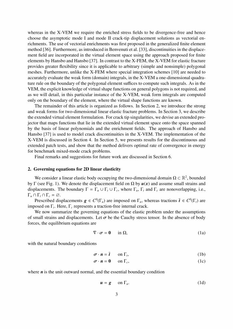
We consider a linear elastic body occupying the two-dimensional domain Ω ⊂ R2, boundedby Γ (see Fig. 1). We denote the displacement field on Ω by u(x) and assume small strains anddisplacements. The boundary Γ = Γu ∪ Γt ∪ Γc, where Γu, Γt and Γc are nonoverlapping, i.e.,Γu ∩ Γt ∩ Γc = ∅.
Prescribed displacements g ∈ C0(Γu) are imposed on Γu, whereas tractions t ∈ C0(Γt) areimposed on Γt. Here, Γc represents a traction-free internal crack.
We now summarize the governing equations of the elastic problem under the assumptionsof small strains and displacements. Let σ be the Cauchy stress tensor. In the absence of bodyforces, the equilibrium equations are
∇ · σ = 0 in Ω, (1a)
with the natural boundary conditions
σ · n = t on Γt, (1b)σ · n = 0 on Γc, (1c)
where n is the unit outward normal, and the essential boundary condition
u = g on Γu. (1d)
3
Γc
Γu
Γt
Ω
Γ
t
Figure 1: Elastostatic boundary-value problem for an embedded crack.
The small strain tensor ε is related to the displacement field u by the compatibility equation
ε(u) = ∇su, (1e)
where ∇s is the symmetric part of the gradient operator, which is defined as
∇s(·) =12
(∇(·) + ∇T (·)
).
Lastly, the isotropic linear elastic constitutive law is
σ(u) = C : ε(u), (1f)
where C is the fourth-order elasticity tensor for a homogeneous isotropic material.The weak form of the problem is constructed by defining the space of admissible displace-
ment fields as
U =v ∈ [H1(Ω)]2 : v = g on Γu, v discontinuous on Γc
, (2)
where the space V is related to the regularity of the solution, and admits discontinuous functionsacross the crack. Similarly, the test function space is defined as:
U0 =v ∈ [H1(Ω)]2 : v = 0 on Γu, v discontinuous on Γc
. (3)
The weak form of the equilibrium equation reads as: Find u ∈ U such that
a(u, v) :=∫
Ω
σ(v) : ε(u) dx =
∫Γt
t · vdΓ =: b(v) ∀v ∈ U0. (4)
The above statement is equivalent to the strong form (1a) and in a finite element framework itis solved approximately on a sequence of appropriately nested finite-dimensional subspaces ofU .
4
3. Extended virtual element formulation
We now discuss the formulation of the extended virtual element method for two-dimensionalelasticity problems. We start, in Section 3.1, from the definition and regularity properties of themesh families for the X-VEM, and after reviewing the ‘nonenriched’ VEM in Section 3.2, weprovide the design of the X-VEM for full and partial local enrichments in Sections 3.3 and 3.4.
3.1. Mesh definition and regularity assumptionsLet T = Ωhh be a family of decompositions of Ω into nonoverlapping polygonal elements
E with nonintersecting boundary ∂E, barycenter xE ≡ (xE, yE)T , area |E|, and diameter hE =
supx,y∈E |x − y|. The subindex h that labels each mesh Ωh is the maximum of the diameters hE
of the elements of that mesh. The boundary of E is formed by NE straight edges connecting NE
vertices. The sequence of the vertices on ∂E is oriented in the counter-clockwise order and thevertex coordinates are denoted by xi ≡ (xi, yi)T , i = 1, 2, . . . ,NE. We denote the unit normalvector to ∂E pointing out of E by nE.
Usually, in the convergence analysis of the conforming VEM, it is assumed that there existsa positive constant % independent of h (hence, also of Ωh) such that for every polygonal elementE ∈ Ωh it holds that:
(i) E is star-shaped with respect to a disk with radius greater than %hE;(ii) for every edge e ∈ ∂E it holds that he ≥ %hE.
Although the convergence analysis of the X-VEM is beyond the scope of this paper, wepresent such mesh regularity assumptions to characterize the geometry of the elements in thepolygonal meshes, which is pertinent to our formulation. We also note that condition (i) impliesthat all the mesh elements have a finite number of vertices and edges for h → 0 and are simplyconnected subset of R2. In turn, condition (ii) excludes the possibility of collapsing vertices inthe refinement process, i.e., vertices whose distance becomes zero faster than h.
3.2. Conforming virtual element space, elliptic projection and bilinear formLet Γc = ∅. On every polygonal element E with boundary ∂E, we first define the following
scalar virtual element space
Vh(E) ≡vh ∈ H1(E) : ∆vh = 0, vh
|∂E ∈ C0(∂E), vh|e ∈ P
1(e) ∀e ∈ ∂E), (5)
where P1(e) is the set of linear polynomials on the element edge e ∈ ∂E and ∆ is the Laplaceoperator. We denote the canonical basis of Vh(E) by ϕi
NEi=1, so that each ϕi is the harmonic
function on E with continuous piecewise linear trace on the boundary ∂E that takes value 1 onthe i-th node and 0 on the remaining nodes. The linear polynomials P1(E) are a subspace ofVh(E), and the basis functions ϕi satisfies the partition-of-unity property
NE∑i=1
ϕi(x) = 1 ∀x ∈ E. (6)
For the linear elasticity (vectorial) problem, on every polygonal element E ∈ Ωh we definethe local virtual element space of vector-valued functions as Vh(E) =
[Vh(E)
]2. Every vector-valued virtual element function vh ∈ Vh(E) is uniquely characterized by its vertex values, also
5
known as the degrees of freedom (DOFs) of the method. In the framework of two-dimensionalelasticity, such degrees of freedom represent the two components of the displacement field atthe mesh vertices. Therefore, we have 2NE degrees of freedom per mesh element E. Suchdegrees of freedom are unisolvent in Vh(E) [15].
We define the set of ‘canonical’ basis functions of Vh(E) byϕi
2NEi=1 so that ϕ2i−1 = (ϕi, 0)T
and φ2i = (0, ϕi)T for i = 1, . . . ,NE. These functions are made explicit by the following expres-sion
Vh(E) = span(
ϕ1
0
),
(0ϕ1
), . . . ,
(ϕi
0
),
(0ϕi
), . . . ,
(ϕNE
0
),
(0ϕNE
), (7)
and the partition-of-unity property (6) implies that
NE∑i=1
ϕ2i−1(x) =
( ∑NEi=1 ϕi(x)
0
)=
(10
)and
NE∑i=1
ϕ2i(x) =
(0∑NE
i=1 ϕi(x)
)=
(01
)∀x ∈ E.
We collect all the element spaces Vh(E) in a conforming way and define the global virtualelement space Vh ⊂ U0 as follows
Vh =vh ∈
[H1(Ω)
]2 : vh|E ∈ Vh(E) ∀E ∈ Ωh
.
Let ah(·, ·) and bh(·) denote computable counterparts of the exact bilinear form a(·, ·) and thelinear functional b(·) acting on Vh, and consider the virtual element affine subspace of Vh givenby
Vhg =
vh ∈ Vh : vh = gh on Γu
,
which incorporates the essential boundary condition (1d) in the space definition by taking thelinear interpolant gh of g, and the linear subspace Vh
0 ⊂ Vh that is obtained by setting gh = 0 inVh
g. With this caveat, the virtual element approximation of the variational problem (4) reads as:Find uh ∈ Vh
g such that
ah(uh, vh) = bh(vh) ∀vh ∈ Vh0. (8)
To construct the bilinear form ah(·, ·) and the linear functional bh(·), we first split them asthe sum of element terms ah,E(·, ·) and bh,E(·) so that
ah(uh, vh) =∑E∈Ω
ah,E(uh, vh) ∀uh, vh ∈ Vh,
bh(uh) =∑E∈Ω
bh,E(vh) ∀vh ∈ Vh.
It is well established in the VEM literature that a crucial requirement for every ah,E(·, ·)to deliver an accurate and stable formulation is to satisfy the properties of linear consistencyand stability [12]. To construct such ah,E(·, ·), we resort to the elliptic projection operatorΠa : Vh(E) →
[P
1(E)]2, which maps vector-valued functions from Vh(E) onto linear vector
6
polynomials. To fix the nontrivial kernel in the definition of such elliptic projector, we intro-duce the average translation operator over the NE element vertices
x j
NEj=1 defined as
w =1
NE
NE∑j=1
w(x j), (9)
and the average rotation operator defined as
(w)R =1
NE
NE∑j=1
r(x j) · w(x j), r(x) =(y,−x
)T. (10)
For each vh ∈ Vh(E), the elliptic projection Πa(vh) is the solution of the variational problem∫Eσ(q) : ε(Πavh) dx =
∫Eσ(q) : ε(vh) dx ∀q ∈
[P
1(E)]2, (11a)
with the additional conditions
Πavh = vh, (11b)
(Πavh)R = (vh)R. (11c)
Conditions (11b) and (11c) fix the rigid-body modes (two translations and one rotation) thatform the kernel of ε(·).
A requirement for such a projection operator is that it is computable from the degrees offreedom of Vh, as we explain below. In order to compute Πa(vh) it is convenient to choose, as abasis of P1(E), the set of scaled monomials
m(x) =1, ξ(x), η(x)
, with ξ(x) =
x − xE
hE, η(x) =
y − yE
hE, (12)
where x =(x, y
)T , so that the basis functions of P1(E) scale as O(1) with respect to h. Itimmediately follows that P1(E) = span1, ξ, η, and a possible basis of
[P
1(E)]2 is
[P
1(E)]2
= span(
10
),
(01
),
(η−ξ
),
(ξ0
),
(0η
),
(ηξ
). (13)
The six vector fields in (13) represent the three planar rigid-body modes and the three indepen-dent nonzero deformation modes.
To prove the computability of Πa, we rewrite (11a) with (11b)-(11c) as a linear system. Forevery ϕi from the canonical basis of Vh(E) shown in (7), we consider the expansion of Πaϕi onthe basis of [P1(E)]2 shown in (13). A suitable application of the divergence theorem showsthat Πaϕi is computable by using only the degrees of freedom of ϕi and noting that ∇·σ(ϕi) = 0.The polynomial projection Πavh can readily be computed for all virtual element fields vh fromthe projections of the basis functions ϕi because the projection operator is a linear operator.
We will expand on this observation in the next section.
7
Once computed, operator Πa allows us to evaluate the local approximated bilinear form asfollows
ah,E(vh,wh) = aE(Πa(vh), Πa(wh))
+ S E((vh − Πa(vh)),(wh − Πa(wh)
))=
∫Eσ(Πa(vh)) : ε(Πa(wh) dx + S E((vh − Πa(vh)
),(wh − Πa(wh)
)),
where S E(·, ·) is a suitable stabilizing term that preserves the coercivity of the system. Accordingto the virtual element methodology, S E(·, ·) can be any symmetric, positive definite, continuousbilinear form defined on the kernel of the projection operator Πa [12].
We refer the reader to Section 4 for possible choices of the stabilization term.
Finally, the expression for the virtual element approximation of the linear functional in theright-hand side of (8) is given by
bh,E(vh) =
∫Γt∩∂E
t · vh dΓ = bE(vh),
where bh,E(vh) is computable because t is known and the trace of vh is a linear polynomial oneach edge e ∈ Γt ∩ ∂E that is known through the interpolation of the edge degrees of freedom.
3.3. Extended virtual element space, elliptic projection and bilinear formIf the exact solution to the selected problem contains singularities, then similar to the finite
element method, the accuracy of the virtual element method is compromised. For this reason,it is beneficial to enrich the virtual element space by means of independent fields carryinginformation about the singularities affecting the exact solution. As we discuss later on, suchfields are required to satisfy the equilibrium equations (1a). For two-dimensional elastic fractureproblems, we choose the enrichment fields as a scaled form of the exact asymptotic crack-tipdisplacement fields for mode I and mode II crack opening, uI =
(uI
x, uIy)T and uII =
(uII
x , uIIy )T ,
respectively. These enrichment fields are given by the expressions:
uIx := uI
x(r, θ) =
√r
2π
[(2κ − 1) cos
(θ
2
)− cos
(3θ2
)], (14a)
uIy := uI
y(r, θ) =
√r
2π
[(2κ + 1) sin
(θ
2
)− sin
(3θ2
)], (14b)
uIIx := uII
x (r, θ) =
√r
2π
[(2κ + 3) sin
(θ
2
)+ sin
(3θ2
)], (14c)
uIIy := uII
y (r, θ) = −
√r
2π
[(2κ − 3) cos
(θ
2
)+ cos
(3θ2
)], (14d)
where (r, θ) are polar coordinates in the local crack tip reference system (see Fig. 2) and κ is theKolosov constant.
An explicit computation implies that these fields satisfy equilibrium, i.e., the conditions∇·σ(uI) = 0 and ∇·σ(uII) = 0 hold. Note that uI and uII belong to H
32−η(Ω) for any η > 0 [38],
8
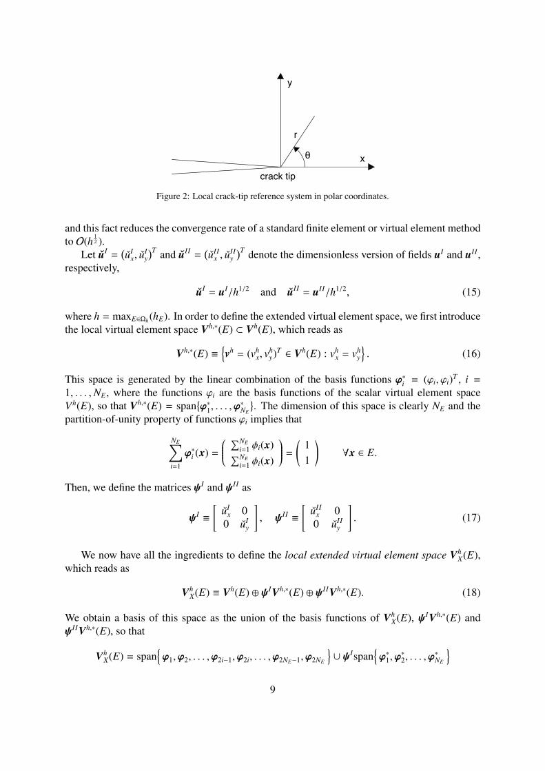
crack tip
x
y
θ
r
Figure 2: Local crack-tip reference system in polar coordinates.
and this fact reduces the convergence rate of a standard finite element or virtual element methodto O(h
12 ).
Let uI =(uI
x, uIy)T and uII =
(uII
x , uIIy)T denote the dimensionless version of fields uI and uII ,
respectively,
uI = uI/h1/2 and uII = uII/h1/2, (15)
where h = maxE∈Ωh(hE). In order to define the extended virtual element space, we first introducethe local virtual element space Vh,∗(E) ⊂ Vh(E), which reads as
Vh,∗(E) ≡vh = (vh
x, vhy)T ∈ Vh(E) : vh
x = vhy
. (16)
This space is generated by the linear combination of the basis functions ϕ∗i = (ϕi, ϕi)T , i =
1, . . . ,NE, where the functions ϕi are the basis functions of the scalar virtual element spaceVh(E), so that Vh,∗(E) = span
ϕ∗1, . . . ,ϕ
∗NE
. The dimension of this space is clearly NE and the
partition-of-unity property of functions ϕi implies that
NE∑i=1
ϕ∗i (x) =
∑NEi=1 φi(x)∑NEi=1 φi(x)
=
(11
)∀x ∈ E.
Then, we define the matrices ψI and ψII as
ψI ≡
[uI
x 00 uI
y
], ψII ≡
[uII
x 00 uII
y
]. (17)
We now have all the ingredients to define the local extended virtual element space VhX(E),
which reads as
VhX(E) ≡ Vh(E) ⊕ ψIVh,∗(E) ⊕ ψIIVh,∗(E). (18)
We obtain a basis of this space as the union of the basis functions of VhX(E), ψIVh,∗(E) and
ψIIVh,∗(E), so that
VhX(E) = span
ϕ1,ϕ2, . . . ,ϕ2i−1,ϕ2i, . . . ,ϕ2NE−1,ϕ2NE
∪ ψIspan
ϕ∗1,ϕ
∗2, . . . ,ϕ
∗NE
9
∪ ψIIspanϕ∗1,ϕ
∗2, . . . ,ϕ
∗NE
, (19)
where we recall that ϕ2i−1 = (ϕi, 0)T , ϕ2i = (0, ϕi)T and ϕ∗i = (ϕi, ϕi)T , i = 1, . . . ,NE. Therefore,at every enriched node the vector-valued field vh
X(x) that belongs to the extended virtual elementspace Vh
X(E) is characterized by four values and for an element whose nodes are all enriched,we have 4NE degrees of freedom. For example, at the j-th node with coordinates x j, we findthat
vh(x j) =
NE∑i=1
[vh
i,x
(ϕi(x j)
0
)+ vh
i,y
(0
ϕi(x j)
)+ vh
i,I
uIx(x j)ϕi(x j)
uIy(x j)ϕi(x j)
+ vhi,II
uIIx (x j)ϕi(x j)
uIIy (x j)ϕi(x j)
]
=
vhj,x + vh
j,I uIx(x j) + vh
j,I uIIx (x j)
vhj,y + vh
j,II uIy(x j) + vh
j,II uIIy (x j)
,since ϕi(x j) = δi j.
Remark 3.1. Here, vhi,x, vh
i,y, vhi,I and vh
i,II are the coefficients of the basis functions in (19) andcan thus be identified with the degrees of freedom of the method. Note, however, that the degreesof freedom of an enriched function vh
X ∈ VhX(E) are no longer the values of vh
X at the vertices ofelement E.
To ease the exposition, we denote the basis functions of VhX(E) by the symbol ϕi, i =
1, 2, . . . , 4NE, so that VhX(E) = span
ϕ1, ϕ2, . . . , ϕ4NE
where
ϕi =
(ϕi, 0
)Tfor 1 ≤ i ≤ 2NE, i odd,(
0, ϕi
)Tfor 1 ≤ i ≤ 2NE, i even,(
uIxϕi, uI
yϕi
)Tfor 1 + 2NE ≤ i ≤ 3NE,(
uIIx ϕi, uII
y ϕi
)Tfor 1 + 3NE ≤ i ≤ 4NE.
Finally, the extended global virtual element space VhX is defined as follows:
VhX =
vh
X ∈[H1(Ω)
]2 : vhX |E ∈ Vh
X(E) ∀E ∈ Ωh
.
Again, to consider the essential boundary condition (1d) we consider the affine subspace VhX,g
of VhX defined by
VhX,g =
vh
X ∈ VhX : vh
X = ghX on Γu
,
where ghX is the extended linear interpolant of g, and the linear subspace Vh
X,0, which is definedby setting gh
X = 0 in the above definition.Since ϕi
4NEi=1 are not known in the interior of the element, we construct a convenient projec-
tion operator that will allow us to obtain computable approximations ahX(·, ·) : Vh
X(E)×VhX(E)→
R and bhX(·) : Vh
X(E)→ R of the exact bilinear form a(·, ·) and the linear functional b(·) appear-ing in (4). The extended virtual element formulation then reads: Find uh
X ∈ VhX,g such that
ahX(uh
X, vhX) = bh
X(vhX) ∀vh
X ∈ VhX,0, (20)
10
where the bilinear form ahX(·, ·) is built element-wise as
ahX(uh
X, vhX) =
∑E∈Ω
ah,EX (uh
X, vhX) ∀uh
X, vhX ∈ Vh
X, (21)
and again we set bhX(vh
X) = b(vhX).
In order to construct a consistent and stable bilinear form ah,EX (·, ·), we extend the polyno-
mial space P1(E) to a subspace of Vh(E) including the linear polynomials and the additionalenrichment functions uI and uII , so that
PX(E) ≡ P1(E) ⊕ span(uI , uII).
Space PX(E) is spanned by the eight linearly independent vector fields
PX(E) = span (
10
),
(01
),
(η−ξ
),
(ξ0
),
(0η
),
(ηξ
),
(uI
xuI
y
),
(uII
xuII
y
) . (22)
The first six vector fields in (22) represent the three fundamental rigid body motions and thethree independent deformation modes that form P
1(E), cf. (13). The last two vector fields arethe scaled enrichment fields chosen to construct the extended virtual element space Vh
X(E).
Remark 3.2. All qX ∈ PX(E) satisfy the equilibrium equation ∇ · σ(qX) = 0. This property iscrucial to determine the computability of the extended projection operator Πa
X.
To construct a bilinear form ah,EX (·, ·) for which such properties hold, we define the extended
elliptic projection operator ΠaX : Vh
X(E)→ PX(E) for each element E. For each vhX ∈ Vh
X(E), theextended elliptic projection Πa
X(vhX) is the solution of the variational problem∫
Eσ(qX) : ε(Πa
XvhX) dx =
∫Eσ(qX) : ε(vh
X) dx ∀qX ∈ PX(E), (23a)
with the additional conditions
ΠaXvh
X = vhX, (23b)
(ΠaXvh
X)R = (vhX)R, (23c)
where (·) and (·)R are the average translation and rotation, respectively, which are defined in (9)and (10). Recalling the divergence theorem and Remark 3.2, the vector polynomial Πa
XvhX ∈
PX(E) is computable from the degrees of freedom of vhX.
The projection operator ΠaX allows us to define the local extended bilinear form as follows:
ah,EX (vh
X,whX) ≡ aE
(Πa
X(vhX), Πa
X(whX)
)+ S E
X
(vh
X − ΠaX(vh
X), whX − Πa
X(whX)
)=
∫Eσ(Πa
X(vhX)
): ε
(Πa
X(whX)
)dx + S E
X
(vh
X − ΠaX(vh
X), whX − Πa
X(whX)
), (24)
where S EX(·, ·) is a stabilization term that must be suitably defined to guarantee linear consis-
tency (cf. (25)) and stability (cf. (26)) of the method. Again, according to the virtual element
11
methodology, S EX(·, ·) can be any symmetric, positive definite, continuous bilinear form defined
on the kernel of the extended projection operator ΠaX [15]. The reader is referred to Section 4
for possible choices of the stabilization term.With a suitable choice of the stabilization term, the bilinear form ah,E
X (·, ·) has the followingproperties, which are fundamental in order to guarantee the convergence of the method:
(i) extended linear consistency: for all vhX ∈ Vh
X(E) and qX ∈ PX(E) it holds that
ah,EX (vh
X, qX) = aE(vhX, qX); (25)
(ii) stability: there exist two positive constants α∗, α∗, independent of h and E, such that
α∗aE(vhX, v
hX) ≤ ah,E
X (vhX, v
hX) ≤ α∗aE(vh
X, vhX) ∀vh
X ∈ VhX(E). (26)
According to the virtual element theory, cf. [12], the constants α∗ and α∗ must be independentof the mesh size parameter h. However, they can depend on the other model and discretizationparameters such as the bound on C and the mesh regularity constant ρ. Here, aE(·, ·) is the localcoercive and continuous bilinear form
aE(u, v) =
∫Eσ(v) : ε(u) dx ∀u, v ∈ U0.
Remark 3.3. In Section 4, we provide two possible choices of the stabilization term by consid-ering the standard dofi-dofi and D-recipe formulations in our extended setting. Such choicesare widely accepted in the VEM literature and in some cases they were theoretically proved tobe effective to guarantee stability relations such as (26). However, the choice of the stabilizationterm in the presence of enrichment functions and its impact on the behavior of the VEM are stillopen issues at this time. For example, it would be desirable that the constants of the stabilityrelation (26) are independent of the Young’s modulus and Poisson’s ratio to realize a robustdiscretization. These topics will be the subject of future work.
3.4. Partial enrichmentLet E denote an element of mesh Ωh and kE a positive integer number strictly less than NE
(the case for kE = NE is the full enrichment case). We select kE distinct nodes of element E to beenriched and the corresponding basis functions ϕ∗i` ∈ Vh,∗(E) labeled by the kE distinct indicesi` ∈ [1,NE] for ` = 1, . . . , kE. We formally denote the subset of these indices by I = i`
kE`=1.
Using these basis functions, we define the reduced virtual element space
Vh,∗
(E) ≡ spanϕ∗i1 ,ϕ
∗i2 , . . . ,ϕ
∗ikE
⊂ Vh,∗(E)
and the reduced extended virtual element space
VhX(E) = Vh(E) ⊕ ψIV
h,∗(E) ⊕ ψIIV
h,∗(E) ⊂ Vh
X,
where a tilde accent as a superscript is used to denote all ‘reduced’ mathematical objects. Equiv-alently, we can define the reduced virtual element space V
hX(E) as the span of the basis functions
of Vh(E), ψIVh,∗
(E) and ψIIVh,∗
(E), so that
VhX(E) = span
ϕ1,ϕ2, . . . ,ϕ2i−1,ϕ2i, . . . ,ϕ2NE−1,ϕ2NE
∪ ψIspan
ϕ∗1,ϕ
∗2, . . . ,ϕ
∗kE
12
∪ ψIIspanϕ∗1,ϕ
∗2, . . . ,ϕ
∗kE
, (27)
which can be compared to (19). Accordingly, a generic virtual element function that belongs tothe reduced space V
hX(E) is described by 2NE + 2kE degrees of freedom instead of 4NE degrees
of freedom. The first 2NE degrees of freedom are the vertex values of a vector-valued fieldvh ∈ Vh(E). The other 2kE degrees of freedom correspond to the vertex values of a virtual vector-valued function that belongs to the enriching space ψIV
h,∗(E) ⊕ ψIIV
h,∗(E) and clearly depends
on uI and uII . We outline a few important facts that will be crucial in the implementationof the partially enriched virtual element method. First, the set of basis functions ϕ∗i` for ` =
1, . . . , kE does not satisfy a partition-of-unity property. Consequently, the enriching fields uI
and uII are not elements of ψIVh,∗
(E) ⊕ ψIIVh,∗
(E) and the extended space PX(E) cannot be a
subspace of Vh,∗
(E). However, since VhX(E) is a linear subspace of Vh
X(E), we can still apply theprojection operator Πa
X to its functions and obtain a projection in the extended spacePX(E), andthe construction of the bilinear form ah,E
X (·, ·) of the previous section still holds. For a proper
formal definition, we introduce the extension (or injection) operator EkE : Vh,∗
(E) → Vh,∗(E)that remaps any reduced virtual element function vh
X ∈ VhX(E) into the fully enriched function
EkE (vhX) ∈ Vh
X(E) such that:
i-th DOF of EkE (vhX) =
i-th DOF of vh
X if 1 ≤ i ≤ 2NE,
i`-th DOF of vhX if i = 2NE + i` or i = 3NE + i` with i` ∈ I,
0 otherwise.
(28)
Practically speaking, the remapped function has the same degrees of freedom of the reducedfunctions and zero at all the additional degrees of freedom that correspond to the nonenrichednodes. Then, we define a new stiffness bilinear form ah,E
X (·, ·) : VhX(E) × V
hX(E)→ R as
ah,EX
(vh
X, whX
):= ah,E
X
(EkE
(vh
X),EkE
(wh
X)), (29)
so that we can reuse the definition of ah,EX (·, ·). Furthermore, the whole construction of the
previous section, including the consistency and stability properties, still holds.
As we discuss in the implementation section, this formal approach also suggests a straight-forward way (but perhaps not the most efficient one) to implement the partial enrichment as allwe need in practice is to apply a matrix representation of the injection operator EkE to the ele-ment stiffness matrix of a fully enriched element. We will see that this procedure is equivalentto first constructing the fully enriched stiffness matrix, and then simply suppressing all rows andcolumns that correspond to the degrees of freedom of the nonenriched nodes.
As we note in Section 5, partial enrichment induces a loss of optimal convergence, whichalso occurs in the X-FEM. This consequence is not surprising, since even though we are pro-jecting onto a space consisting of polynomials and nonpolynomial near-tip enrichment fields, inthis case the local extended virtual element space is not sufficiently rich to approximate the sin-gular behaviour of the function near the crack tip. Special enrichment strategies can be devisedto overcome this issue, for instance using the so-called geometric enrichment.
13
3.5. Embedding discontinuitiesIn this section, we show how both the regular and the extended virtual element formulations
presented in Sections 3.2 and 3.3 can be endowed with a structure that allows discontinuousfields to be embedded within the virtual element space. Consider a crack γ that intersects someof the elements in a mesh, and define d(x) as the signed distance from a point x to γ. Formodeling strong discontinuities like a crack, it would be convenient to consider enrichmentwith the generalized Heaviside function H(x), which is equal to +1 for points with d(x) ≥ 0 (xis on or above the crack) and −1 for points with d(x) < 0 (x is below the crack). As in the X-FEM, we could enrich those nodes whose basis function’s support intersects the interior of thecrack (not including the tips) with H(x). However, the resulting extended projection Πa
X ontoPX(E) would not be directly computable from the degrees of freedom of the method becausethe corresponding enriched virtual element basis functions Hϕi are not known along the crack.
To deliver a viable solution, we let the element E to be partitioned by the discontinuity γinto two subdomains E− and E+. Following [33], in order to represent two independent linearpolynomials on E− and E+, we adopt the approach of Hansbo and Hansbo [37] and tailor it tothe X-VEM. It is known that the approach of Hansbo and Hansbo is equivalent to the standardX-FEM approximation with Heaviside enrichment [39]. To this end, let NVE
dofs denote the numberof degrees of freedom for element E, such that NVE
dofs = 2NE for the virtual element formulationin 3.2 and NVE
dofs = 4NE for the extended virtual element formulation in Section 3.3. Each oneof the NVE
dofs virtual shape functions, ϕi on E, is written as the sum of two new virtual shapefunctions ϕ−i and ϕ+
i that are both discontinuous across the crack, and are defined as follows:
ϕ+i =
0 in E−
ϕi in E+, ϕ−i =
ϕi in E−
0 in E+. (30)
Clearly, ϕ−i and ϕ+i are harmonic and continuous functions in E− and E+, respectively, and
ϕi = ϕ−i +ϕ+i . Proceeding likewise for all the degrees of freedom in the element, we can generate
NHHdofs = 2NVE
dofs discontinuous functions, starting from the initial NVEdofs virtual basis functions. This
choice implies doubling the nodal DOFs of the element. Therefore, the number of degrees offreedom for the element with an internal discontinuity is twice that of the original element, anda virtual element basis is constructed by considering two copies of the original virtual elementbasis functions, restricted to E− and E+ respectively, as defined in (30).
We now define the local virtual element space to which the discontinuous approximate solu-tion belongs. For the sake of simplicity, we present the derivation with respect to the formulationpresented in Section 3.2. Consider the following spaces:
Vh,−(E) ≡
vh ∈[H1(E−)
]2 : ∆vh|E− = 0, vh
|∂E− ∈ [C0(∂E−)]2,
vh|e ∈
[P
1(e)]2∀e ∈ (∂E ∩ ∂E−), vh
|E+ = 0,
Vh,+(E) ≡
vh ∈[H1(E+)
]2 : ∆vh|E+ = 0, vh
|∂E+ ∈ [C0(∂E+)]2,
vh|e ∈
[P
1(e)]2∀e ∈ (∂E ∩ ∂E+), vh
|E− = 0.
Then, the local virtual element space reads:
VhX(E) ≡
vh
X = (vh,− + vh,+) : vh,− ∈ Vh,−(E), vh,+ ∈ Vh,+(E). (31)
14
Remark 3.4. The space VhX(E) in (31) is not a subspace of H1(E) as we do not assume any
regularity of the virtual element functions across the crack, so that a discontinuity is admissible.This fact implies that also the global virtual element space Vh
X cannot be a subspace of H1(Ω),but this is not an issue since the exact solution contains a discontinuity and thus cannot be inH1(Ω).
An analogous definition of the local virtual element space for elements cut by a crack canbe easily provided also for the enriched formulation presented in Section 3.3.
As we detail later on, virtual element functions along interface edges can be reconstructedby a suitable approximation. We obtain the following representation for the virtual elementapproximation on the element E cut by γ:
vhX(x) =
NVEdof∑
i=1
[ϕ−i (x)v−i + ϕ+
i (x)v+i]∀x ∈ E, (32)
where v−i and v+i are the degrees of freedom associated with ϕ−i and ϕ+
i , respectively. To providea feasible solution using (32), it is necessary to know the trace of the virtual shape functions ϕialong the crack. We also need two distinct regular projectors, respectively Πa,− onto
[P
1(E−)]2
and Πa,+ onto[P
1(E+)]2, and two distinct extended projectors, respectively Πa,−
X onto PX(E−)and Πa,+
X onto PX(E+). These projection operators must be computable from the NHHdof nodal
degrees of freedom. A convenient approximation of the trace of the i-th virtual element shapefunction ϕi along the crack is provided by a vector-valued function Ni(x), that is componentwiseharmonic on the cracked element E. Such a function is built as a first-order polyharmonicspline [40] and the reader is pointed to [33] for further details.
We also point out that the flexibility of the virtual element method allows an element tobe cut into two polygonal virtual elements, regardless of the element shape, and therefore themodeling of crack opening and growth can follow this alternative route (see [29]). However,mesh quality can be affected. For instance, let us consider the case when partitioning of theelement results in one subelement being a quasi-degenerate triangle: this badly-shaped trianglewill worsen matrix-conditioning and/or the interpolation error. This scenario becomes acute in3D if sliver tetrahedra appear and the partitioning is now much more difficult to handle, bothalgorithmically and computationally. Moreover, a technique to embed a discontinuous field inthe extended virtual element discrete space is required whenever a mesh-independent modelingapproach is preferred, such as in the simulation of cohesive fracture or when a finite elementtransitions from a continuous regime to a region with discontinuous kinematics [41].
4. Numerical implementation
In this section, we outline the main implementation aspects of the extended virtual elementmethod introduced in Sections 3.3–3.5. For the (nonenriched) virtual element formulation pre-sented in Section 3.2, the interested reader can refer to [18].
4.1. Fully enriched elements with singular fieldsTo begin with, we assume a fully enriched element E, i.e., an element in which all the NE
nodes are enriched with the two singular fields (15). Therefore, on such element we have 4NE
15
degrees of freedom, and we can represent any virtual displacement field vhX ∈ Vh
X(E) in termsof the shape functions of Vh
X(E) as vhX = NXdofs
(vh
X)
where dofs(vh
X)∈ R4NE is the vector of
the degrees of freedom of vhX with respect to the basis function ϕi
4NEi=1 spanning Vh
X(E) andNX ∈ R
2×4NE is the matrix whose columns contain such basis functions
NX ≡
[ϕ1
00ϕ1
. . .
. . .uI
xϕ1
uIyϕ1
uIxϕ2
uIyϕ2
. . .
. . .uII
x ϕ1
uIIx ϕ1
uIIx ϕ2
uIIy ϕ2
. . .
. . .
]=
[ϕ1 ϕ2 . . . ϕ4NE
]. (33)
Now, we define matrix MX ∈ R2×8, whose columns are the basis vectors mα of PX(E) intro-
duced in (22)
MX ≡
[1 0 η ξ 0 η uI
x uIIx
0 1 −ξ 0 η ξ uIy uII
y
]=
[m1 m2 m3 m4 m5 m6 m7 m8
]. (34)
Hereafter, we conveniently use the notation m7 = uI and m8 = uII . We represent the action ofthe projection operator Πa
X on the virtual basis functions by means of a matrix ΠaX ∈ R
8×4NE .The i-th column of this matrix, denoted by πi =
(πiα
)∈ R8, contains the coefficients of Πa
X(ϕi)when the projection is expanded on the basis MX so that
ΠaX(ϕi) = MXπ
i =
8∑α=1
mαπiα, (35)
which in compact form can be expressed as ΠaX(NX) = MXΠ
aX.
We preliminarily observe that for every qX ∈ PX(E) and every vhX ∈ Vh
X(E), recalling that∇ · σ(qX) = 0 and applying the divergence theorem, we find that
aE(qX, vhX) =
∫Eσ(qX) : ε(vh
X)dx =
∫Eσ(qX) : ∇vh
Xdx
=
∫E∇ · (σ(qX) · vh
X) − vhX · (∇ · σ(qX))dx
=
∫∂E
(σ(qX) · vhX) · nEds (36)
The boundary integral is always computable, since the integrand is known on the boundary.By virtue of (36) and recalling the definition of the elliptic projection operator, we compute
the projections of the virtual shape functions in terms of the basis of PX(E). Indeed, for everyvh
X ∈ VhX(E) we can write the following orthogonality condition:
aE(mβ,ΠaX(vh
X)) = aE(mβ, vhX) β = 1, . . . , 8. (37)
Then, recall that dofs(vh
X)
= (vhX,i) are the 4NE degrees of freedom of vh
X with respect to the basisϕi
4NEi=1 . In view of (35) and noting that vh
X and dofs(vh
X)
are arbitrary, we find that
4NE∑i=1
aE(mβ,ΠaX(ϕi)
)vh
X,i =
4NE∑i=1
aE(mβ,ϕi)vhX,i β = 1, . . . , 8
=⇒
8∑α=1
aE(mβ,mα
)πiα = aE(mβ,ϕi) β = 1, . . . , 8, i = 1, . . . , 4NE
=⇒ GXΠaX = BX,
16

where the companion matrices GX ∈ R8×8 and BX ∈ R
8×4NE are defined componentwise as
(GX)β,α = aE(mβ,mα), β, α = 1, . . . , 8,
(BX)β,i = aE(mβ,ϕi), β = 1, . . . , 8, i = 1, . . . , 4NE,
or in the equivalent compact form by
GX = a(MTX, MX) and BX = a(MT
X, NX). (38)
Recalling (36), both matrices GX and BX can be computed by integrating on the element bound-ary as follows:
(GX)β,α =
∫Eσ(mβ) : ε(mα)dΩ =
∫∂E
(σ(mβ
)· mα
)· nEdΓ, (39)
(BX)β,i =
∫Eσ(mβ) : ε(ϕi)dΩ =
∫∂E
(σ(mβ
)· ϕi
)· nEdΓ. (40)
The first three rows of GX and BX are zero, since the small strain tensor associated to rigidbody motions is zero, and therefore GX is rank deficient. To overcome this issue we use condi-tions (23b)-(23c), which imposes that the projector preserves the average nodal translations androtations. So, we define the matrices GX =
((GX)β,α
)and BX =
((BX)β,i
)as
(GX)β,α =
1NE
NE∑j=1
mα(v j) β = 1, 2,
1NE
NE∑j=1
r(v j) · mα(v j) β = 3,
(GX)β,α β = 4, . . . , 8,
(41)
and
(BX)β,i =
1NE
NE∑j=1
ϕi(v j) β = 1, 2,
1NE
NE∑j=1
r(v j) · ϕi(v j) β = 3,
(BX)β,i β = 4, . . . , 4NE.
(42)
Since matrix GX is nonsingular, the projection matrix ΠaX is the unique solution of the linear
system GXΠaX = BX. To derive the representation of the operator Πa
X with respect to the basisϕi
4NEi=1 spanning Vh
X(E) we introduce matrix DX ∈ R4NE×8, whose α-th column (α = 1, . . . , 8)
contains the degrees of freedom of the vector polynomial mα. Therefore, it holds that MX =
NX DX and
ΠaX(NX) = MXΠ
aX = NX
(DXΠ
aX),
17
from which we infer that such matrix representation is given by matrix DXΠaX. A straight-
forward calculation yields that GX = BX DX in the X-VEM, which is similar in form to thestandard relation in the VEM, G = BD [42]. This provides a means to verify the correctnessof the computation of these matrices.
The stiffness matrix is given by the sum of a consistency and stability term,
KEX = KE
X,c + KEX,s,
so that we can evaluate the extended stiffness bilinear form applied to vhX, wh
X ∈ VhX(E) by using
the degrees of freedom dofs(vh
X)
and dofs(wh
X)
as follows
ah,EX
(vh
X,whX
)=
(dofs
(vh
X))T KE
X dofs(wh
X). (43)
For every vhX ∈ Vh
X(E), we first consider the relations
ΠaX(vh
X) = ΠaX(NXdofs
(vh
X))
= ΠaX(NX
)dofs
(vh
X)
= MXΠaX dofs
(vh
X)
=(dofs
(vh
X))T (Πa
X)T (MX)T .(44)
Recalling (44), we compute the consistency term as
aE(ΠaX(vh
X),ΠaX(wh
X))
=(dofs
(wh
X))T (Πa
X)T aE(MTX, MX
)Πa
Xdofs(vh
X)
=(dofs
(wh
X))T (Πa
X)T GXΠaXdofs
(wh
X).
By comparison, we see that
KEX,c = (Πa
X)T GXΠaX. (45)
For the stability term we generalize the so-called dofi-dofi [12] and D-recipe [43] stabiliza-tions by evaluating the second term in (24) at the element vertices. To this end, we first notethat
vhX(x`) − Πa
X(vhX)(x`) = NX(x`)dofs
(wh
X)− NX(x`)DXΠ
aXdofs
(wh
X).
Definition (33) and ϕ j(x`) = δ j` implies that
j-th column of NX(x`) =
(ϕ j(x`), 0
)Tfor 1 ≤ j ≤ 2NE, j odd,(
0, ϕ j(x`))T
for 1 ≤ j ≤ 2NE, j even,(uI
x(x`)φ j(x`), uIy(x`)ϕ j(x`)
)Tfor 1 + 2NE ≤ j ≤ 3NE,(
uIIx (x`)φ j(x`), uII
y (x`)ϕ j(x`))T
for 1 + 3NE ≤ j ≤ 4NE,
=
(δ j,`, 0
)Tfor 1 ≤ j ≤ 2NE, j odd,(
0, δ j,`
)Tfor 1 ≤ j ≤ 2NE, j even,(
uIx(x`)δ j,`, uI
y(x`)δ j,`
)Tfor 1 + 2NE ≤ j ≤ 3NE,(
uIIx (x`)δ j,`, uII
y (x`)δ j,`
)Tfor 1 + 3NE ≤ j ≤ 4NE,
18
for ` = 1, . . . ,NE. We collect NX(x`) in the compact block-diagonal matrix J = diag(J11, J22) ∈R
4NE×4NE such that J11 = I2NE×2NE , which is the 2NE × 2NE-sized identity matrix, and J22 =[J I
22, J II22], with
J I22 = diag
(uI(x1), uI(x2), . . . , uI(xNE )
),
J II22 = diag
(uII(x1), uII(x2), . . . , uII(xNE )
).
Here, J11 ∈ R2NE×2NE collects the values of the first 2NE columns of NX(x`) and is such that
the `-th row corresponds to the `-th element vertex. In turn, the matrix blocks J I22 and J II
22 are2NE × NE-sized matrices that collect the NE columns of NX corresponding to ψIVh,∗(E) andψIIVh,∗(E), and again each row corresponds to a given element vertex. Finally, we introduce thematrix DX = J DX, and we write the dofi-dofi stabilization as
S EX
(vh
X − ΠaX(vh
X),whX − Πa
X(whX)
)= τ
NE∑`=1
(NX(x`)dofs
(vh
X)− NX(x`)DXΠ
aXdofs
(vh
X))
×(NX(x`)dofs
(wh
X)− NX(x`)DXΠ
aXdofs
(wh
X))
= τ(dofs
(vh
X))T (
J − DXΠaX
)T (J − DXΠ
aX
)(dofs
(wh
X)), (46)
where τ is a suitable scaling parameter; a possible choice is τ = α trace(KEX,c)/4NE, where α is
a constant (a sensitivity analysis on the choice of α is presented in the next section). Hence,
KEX,s = τ(J − DXΠ
aX)T (J − DXΠ
aX).
Similarly, the D-recipe stabilization, which was originally proposed in [43] for the Poissonequation, can be generalized by taking the stabilization matrix
KEX,s = (J − DXΠ
aX)T SX (J − DXΠ
aX),
where
(SX)i j = δi j max(trace(C)
3hE, (KE
X,c)ii
)i, j = 1, . . . ,NE,
and with the same definition of J and DX introduced above.
4.2. Partially enriched elements with singular fieldsLet EX ∈ R
4NE×(2NE+2kE) be the matrix representation of the extension operator EkE intro-duced in Section 3.4, so that every vector-valued field vh
X ∈ VhX(E) with degrees of freedom
dofs(vh
X)∈ R2NE+2kE is remapped into the vector-valued field vh
X ∈ VhX(E) with degrees of free-
dom dofs(vh
X)
= EXdofs(vh
X)∈ R4NE . Let K
EX ∈ R
(2NE+2kE)×(2NE+2kE) such that
ah,EX
(vh
X, whX
)=
(dofs
(vh
X))T K
EX dofs
(wh
X). (47)
19
Now, starting from definition (29) and using (47), a straightforward calculation yields
ah,EX
(vh
X, whX
)= ah,E
X
(EkE vh
X,EkE whX
)=
(dofs
(EkE wh
X))T
KEX dofs
(EkE vh
X)
=(EXdofs
(wh
X))T
KEX EXdofs
(vh
X)
=(dofs
(wh
X))T (
EX)T KE
X EX dofs(vh
X),
and by comparison with (47) it follows that
KEX =
(EX
)T KEX EX, (48)
since vhX and wh
X are arbitrary. To conclude this section, we are only left to explain the con-struction of the matrix EX that embodies definition (28). To obtain such a matrix, we take the4NE×4NE-size identity matrix and remove the 2(NE−kE) columns that corresponds to the basisfunctions of the nonenriched vertices in ψIVh,∗(E) ⊕ ψIIVh,∗(E). Finally we note that when weapply (EX)T to the left of matrix KE
X and EX to the right of matrix KEX we are indeed selecting
the rows and the columns of KEX that corresponds to all the degrees of freedom of Vh(E) and
the degrees of freedom of the enriched nodes of ψIVh,∗(E) ⊕ ψIIVh,∗(E). In the numerical im-plementation we do not need to construct the matrix EX explicitly and compute K
EX using (48),
since we can simply build the stiffness matrix KEX of the full enrichment case and remove all
rows and columns that refer to non-enriched nodal degrees of freedom.
4.3. Embedding discontinuitiesLet us consider the case in which an element E, fully enriched according to the construction
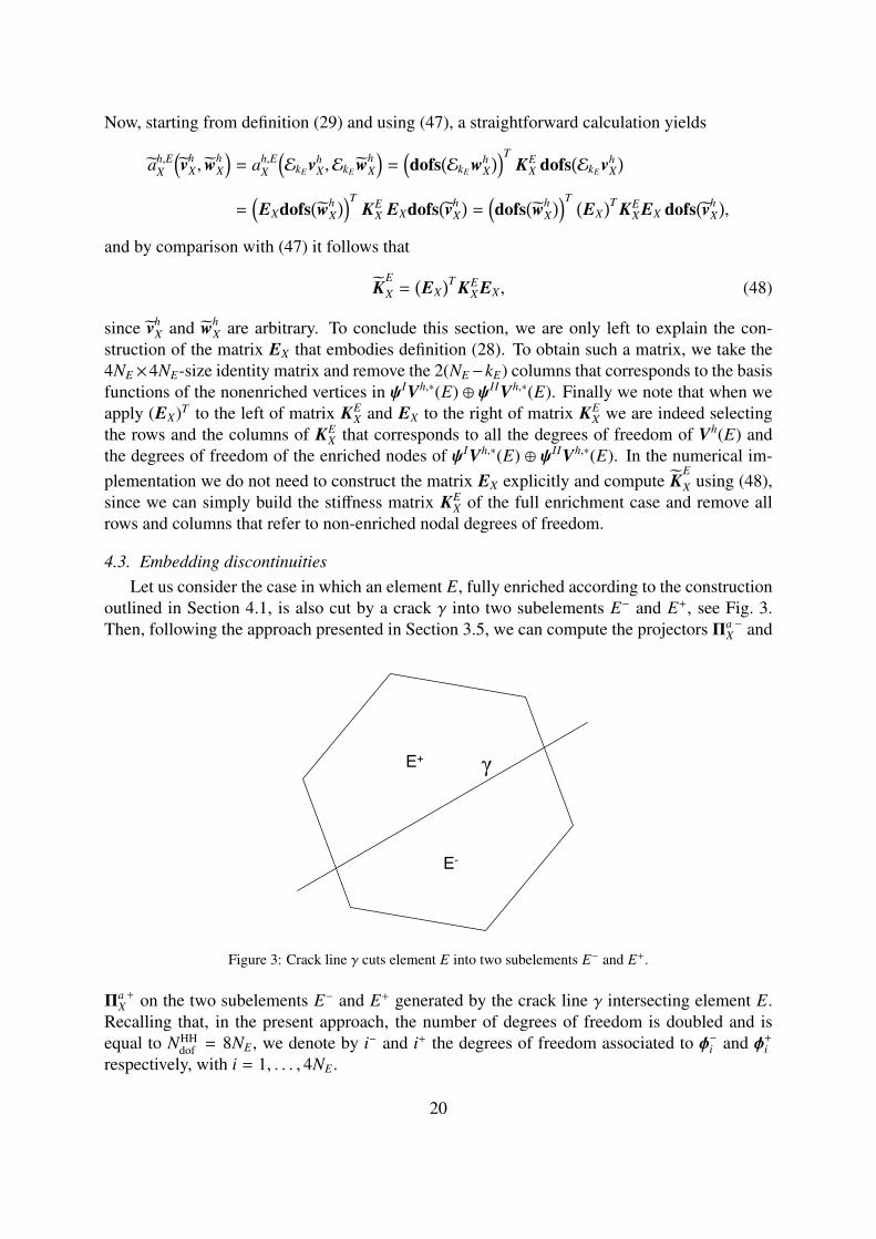
outlined in Section 4.1, is also cut by a crack γ into two subelements E− and E+, see Fig. 3.Then, following the approach presented in Section 3.5, we can compute the projectors Πa
X− and
E+
E-
γ
Figure 3: Crack line γ cuts element E into two subelements E− and E+.
ΠaX
+ on the two subelements E− and E+ generated by the crack line γ intersecting element E.Recalling that, in the present approach, the number of degrees of freedom is doubled and isequal to NHH
dof = 8NE, we denote by i− and i+ the degrees of freedom associated to φ−i and φ+i
respectively, with i = 1, . . . , 4NE.
20
Then, the consistent part of the stiffness matrix has a diagonal block structure and is com-posed by the following submatrix blocks:
(KEX,c)+,+ = (Πa
X+)T G
+
XΠaX
+,
(KEX,c)−,− = (Πa
X−)T G
−
XΠaX−,
where matrices G−
X and G+
X are the counterparts of GX computed for E− and E+, respectively.On the other hand, the general expression for the stabilization part shares the same diagonal
block structures and reads:
(KEX,s)+,+ = τ(J − D
+
XΠaX
+)T (J − D+
XΠaX
+),
(KEX,s)−,− = τ(J − D
−
XΠaX−)T (J − D
−
XΠaX−),
where matrices D−
X and D+
X are the counterparts of DX computed for E− and E+, respectively.
4.4. Computation of stress intensity factorsIn order to determine the susceptibility of a given elastic two-dimensional body to fracture
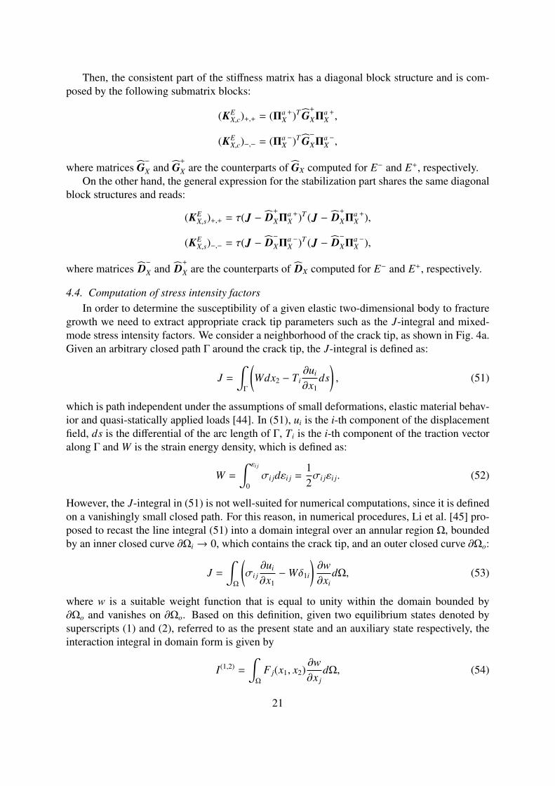
growth we need to extract appropriate crack tip parameters such as the J-integral and mixed-mode stress intensity factors. We consider a neighborhood of the crack tip, as shown in Fig. 4a.Given an arbitrary closed path Γ around the crack tip, the J-integral is defined as:
J =
∫Γ
(Wdx2 − Ti
∂ui
∂x1ds
), (51)
which is path independent under the assumptions of small deformations, elastic material behav-ior and quasi-statically applied loads [44]. In (51), ui is the i-th component of the displacementfield, ds is the differential of the arc length of Γ, Ti is the i-th component of the traction vectoralong Γ and W is the strain energy density, which is defined as:
W =
∫ εi j
0σi jdεi j =
12σi jεi j. (52)
However, the J-integral in (51) is not well-suited for numerical computations, since it is definedon a vanishingly small closed path. For this reason, in numerical procedures, Li et al. [45] pro-posed to recast the line integral (51) into a domain integral over an annular region Ω, boundedby an inner closed curve ∂Ωi → 0, which contains the crack tip, and an outer closed curve ∂Ωo:
J =
∫Ω
(σi j
∂ui
∂x1−Wδ1i
)∂w∂xi
dΩ, (53)
where w is a suitable weight function that is equal to unity within the domain bounded by∂Ωo and vanishes on ∂Ωo. Based on this definition, given two equilibrium states denoted bysuperscripts (1) and (2), referred to as the present state and an auxiliary state respectively, theinteraction integral in domain form is given by
I(1,2) =
∫Ω
F j(x1, x2)∂w∂x j
dΩ, (54)
21
n
Γx1
x2
(a)
rd
(b)
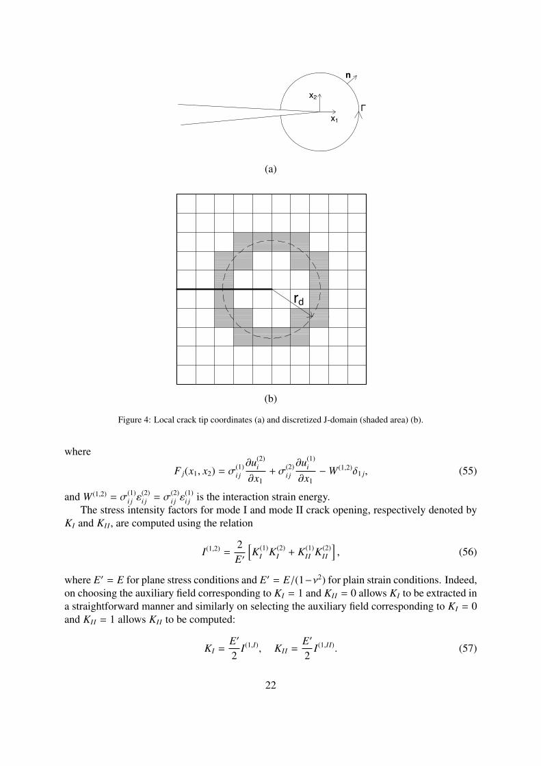
Figure 4: Local crack tip coordinates (a) and discretized J-domain (shaded area) (b).
where
F j(x1, x2) = σ(1)i j
∂u(2)i
∂x1+ σ(2)
i j
∂u(1)i
∂x1−W (1,2)δ1 j, (55)
and W (1,2) = σ(1)i j ε
(2)i j = σ(2)
i j ε(1)i j is the interaction strain energy.
The stress intensity factors for mode I and mode II crack opening, respectively denoted byKI and KII , are computed using the relation
I(1,2) =2E′
[K(1)
I K(2)I + K(1)
II K(2)II
], (56)
where E′ = E for plane stress conditions and E′ = E/(1−ν2) for plain strain conditions. Indeed,on choosing the auxiliary field corresponding to KI = 1 and KII = 0 allows KI to be extracted ina straightforward manner and similarly on selecting the auxiliary field corresponding to KI = 0and KII = 1 allows KII to be computed:
KI =E′
2I(1,I), KII =
E′
2I(1,II). (57)
22
However, computing the interaction integral (54) is not straightforward in the X-VEM, sincethe numerical integration is performed over polygonal elements. For this reason, after consider-ing a J-domain that is an annular region ΩJ that consists of a ring of elements that are intersectedby a circle of given radius rd centered on the crack tip (i.e., the shaded area in Fig. 4b), we ap-ply the divergence theorem and transform the domain integral (54) into a line integral that isevaluated on the boundaries of the element [29]:
I(1,2) =∑E∈ΩJ
(∫∂E
F j(x1, x2)wn jdΓ −
∫E
∂F j
∂x j(x1, x2)wdΩ
). (58)
We note that ∇ · F = 0 in (58) since the auxiliary fields are equilibrated, and therefore only theboundary integral needs to be computed.
Since virtual shape functions are not known in the interior of the elements, we use the ellipticprojection of the solution in terms of displacements to compute the corresponding deformationfield and the stress components. Hence, the interaction integral can be finally computed as:
I(1,2) =∑E∈ΩJ
∫∂E
σi j(ΠaE(u(1)
i ))∂u(2)
i
∂x1+ σ(2)
i j
∂ΠaE(u(1)
i )∂x1
− W (1,2)δ1 j
wn jdΓ, (59)
where W (1,2) = σi j(ΠaE(u(1)
i ))ε(2)i j . From a computational viewpoint, it is convenient to assume
the weight function w to be equal to unity on all nodes in ΩJ that lie within the circle of radiusrd, and equal to zero on all nodes in ΩJ that lie outside the circle of radius rd. Along elementedges, where integrations are carried out, linear interpolation of w between its nodal values isadopted.
5. Numerical examples
In order to check the consistency of the X-VEM, we first conduct two distinct patch tests: anextended patch test, addressing the enrichment with singular fields as described in Section 4.1,and a discontinuous patch test aimed at assessing the inclusion of discontinuities in the discretespace by means of the approach presented in Section 3.5. Then, we test the X-VEM on abenchmark problem to establish the convergence rate of the method and the accuracy of thestress intensity factors. Unless stated otherwise, Young’s modulus E = 105 and Poisson ratioν = 0.3 are chosen in the numerical computations.
5.1. Extended patch testThe extended patch test ensures that the singular enrichment fields in (15) can be exactly
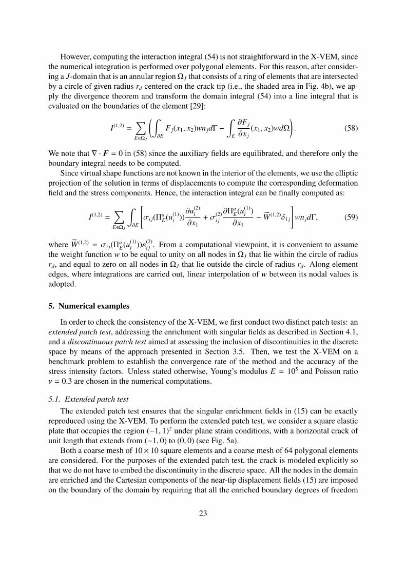
reproduced using the X-VEM. To perform the extended patch test, we consider a square elasticplate that occupies the region (−1, 1)2 under plane strain conditions, with a horizontal crack ofunit length that extends from (−1, 0) to (0, 0) (see Fig. 5a).
Both a coarse mesh of 10× 10 square elements and a coarse mesh of 64 polygonal elementsare considered. For the purposes of the extended patch test, the crack is modeled explicitly sothat we do not have to embed the discontinuity in the discrete space. All the nodes in the domainare enriched and the Cartesian components of the near-tip displacement fields (15) are imposedon the boundary of the domain by requiring that all the enriched boundary degrees of freedom
23
x1
x2
(-1, -1) (1, -1)
(-1, 1) (1, 1)
crack
(a)
-1 -0.5 0 0.5 1x
1
-1
-0.5
0
0.5
1
x 2
(b)
Figure 5: Mixed mode I and mode II crack opening benchmark problem: domain geometry (a) and exact deformedshape (b).
are equal to 1 and all the standard boundary degrees of freedom are equal to 0. The exactdisplacement solution field is shown in Fig. 5b. As detailed in the previous section, integralsneed to be evaluated over the element boundary only. We adopt a 16-points Gauss quadraturerule on each element edge.
As a measure for the error of the numerical solution with respect to the exact solution weadopted the relative error in strain energy, which is computed as
E(uh) =|a(u, u) − a(uh,uh)|
a(u,u), (60)
where 12a(u,u) = 1.6776885579× 10⁻⁵ is the strain energy of the exact solution u, and uh is the
projection of the discrete solution uh, which is defined as:
uh =∑E∈T
ΠaEuh. (61)
We also adopt this error measure in the subsequent sections that follow. In (61), we use the samesymbol Πa
E to denote the restriction of the virtual element functions defined on the element Eof the projection operator Πa if E is a nonenriched element and the projection operator Πa
X if Eis an enriched element. The choice of using the projection uh of the solution uh follows fromobserving that it is not possible to compute the true energy associated with uh, since the virtualfunctions are not explicitly known [46]. The relative error in strain energy for the extendedpatch tests is provided in Table 1, which clearly shows that the X-VEM delivers sound accuracyin reproducing the enrichment fields, although the error is affected by numerical integration ofsingular functions.
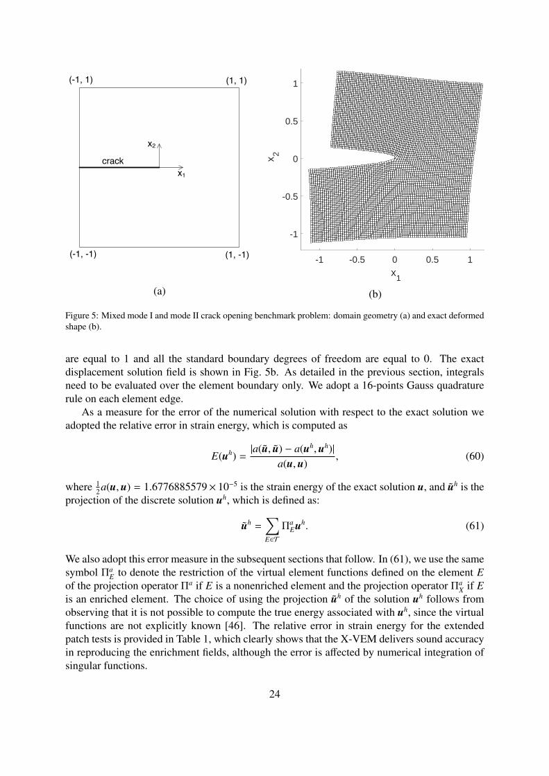
24
Table 1: Relative error in strain energy for the extended patch test on the (−1, 1) × (1, 1) square domain withhorizontal crack.
Mesh E(uh)10 × 10 square elements 2 × 10⁻¹²
64 polygonal elements 3 × 10⁻¹⁰
Figure 6: Geometry and loading conditions of the discontinuous patch test.
5.2. Discontinuous patch testIn order to evaluate the effectiveness and robustness of the X-VEM in the presence of dis-
continuities, formulated according to the approach presented in Section 3.5, we adopt a suit-able patch test which entails solving a problem whose exact solution is discontinuous and liesin the discrete space. We then verify if the extended virtual element approximation matchessuch a solution. To this end, we here adapt the discontinuous patch test first proposed byDolbow and Devan [47] in finite strain elasticity to the present context of plain strain linearelasticity. The test involves solving the problem of a 2D elastic domain occupying the unitsquare domain Ω = (0, 1)2 that is bisected by an horizontal crack γ into two open subdomainsΩ− = (0, 1) × (0, 1/2) and Ω+ = (0, 1) × (1/2, 1). The crack is implicitly included in the modelfollowing the construction proposed in Section 3.5. For the sake of simplicity, we assumeE = 1 and ν = 0, so that the problem is reduced to one dimension. As boundary conditions, weprescribe zero displacements along the edge x = 0, a discontinuous distribution of horizontaltractions along the edge x = 1 and zero tractions along the horizontal edges y = 0 and y = 1:
u(0, y) = 0,
σxx(1, y) =
1, y ≤ 1/22, y > 1/2
, σyy(1, y) = σxy(1, y) = 0,
σyy(x, 0) = σxy(x, 0) = 0,
25
σyy(x, 1) = σxy(x, 1) = 0.
For this problem, whose geometry and boundary conditions are depicted in Fig. 6, the exactsolution is the following piecewise linear function
u(x, y) =
[x, 0]T , (x, y) ∈ Ω− ,
[2x, 0]T , (x, y) ∈ Ω+ .(63)
The exact solution (63) belongs to the discrete space. In agreement with the expectations, theextended virtual element formulation presented in Section 3.5, which uses distinct projectoroperators on the two subdomains generated by the horizontal crack, passes the proposed patchtest with a relative error in strain energy of 2 × 10⁻¹³.
5.3. Convergence studyWe study the convergence of the X-VEM for the problem of a two-dimensional square plate
under plain strain conditions that contains a horizontal crack, extending from the boundary tothe center of the specimen. The boundary conditions are such that mixed-mode conditionsprevail. The geometry of the domain is the same adopted as that for the extended patch testin Section 5.1 and is shown in Fig. 5a. On the boundary of the domain, we apply the exactnear-tip displacement fields (14), which are also employed as enrichment fields for the X-VEMand represent the exact solution for the problem at hand.
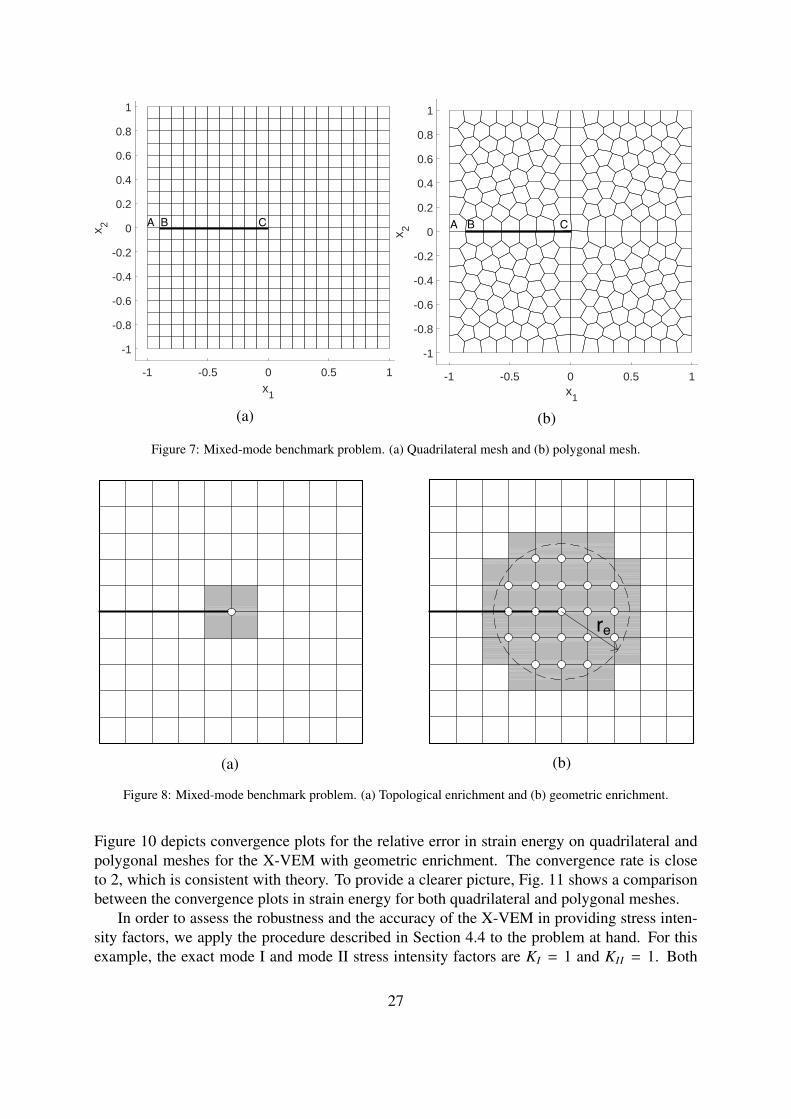
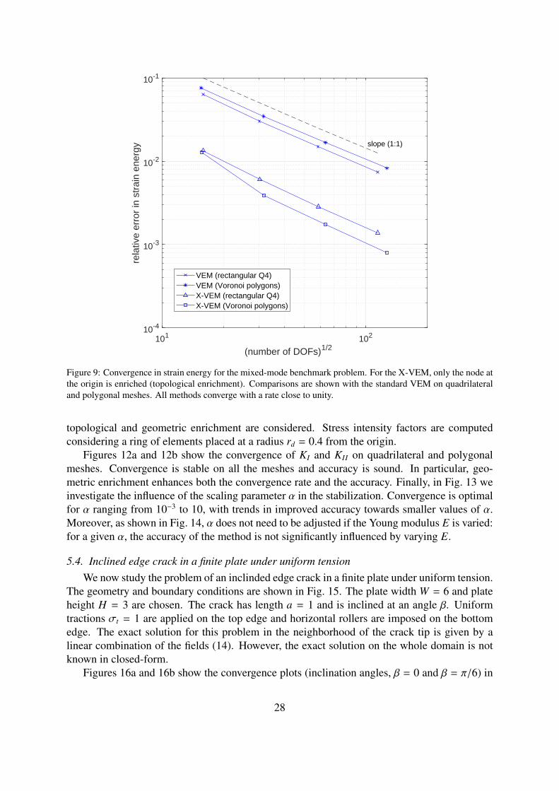
In this study, we consider both quadrilateral and in general polygonal meshes, see Fig.7.Quadrilateral meshes are composed of 10×10, 20×20, 40×40 and 80×80 square elements. Forthe X-VEM, we use the stabilization in (46), where α = 1 is chosen as the scaling parameter.We generated the polygonal meshes from Voronoi tassellations by using Polymesher [48].In order to apply essential boundary conditions, the crack is explicitly meshed over the firstelement (AB), while the remaining part of the crack (BC) is modeled by the X-VEM.
To compute the element stiffness matrix KE, we implement the X-VEM of Section 4 fol-lowing two different strategies: topological enrichment and geometric enrichment. In the topo-logical enrichment, graphically represented in Fig. 8a, we only enrich the node located at thesingularity of the solution. The convergence rate for this problem is given by R = min(2λ, 2p),where λ is the order of the singularity and p the polynomial degree [49]. Since in our caseλ = 1/2 and p = 1, we obtain a convergence rate R = 1 that is non-optimal, as we anticipatedin Section 3.4. In fact, this suboptimal convergence rate is also noted in enriched finite elementtechniques for fracture problems, cf. [50]. Figure 9 shows convergence plots of the relativeerror in strain energy. The expected convergence rate R is reported in the graph. Both VEM andX-VEM with topological enrichment converge in strain energy with a rate close to 1, in agree-ment with theory. It turns out that the X-VEM is insensitive to the type of mesh (quadrilateralsor polygons), and the results from the X-VEM are consistently more accurate than those fromstandard VEM.
Many prior studies have shown that geometric enrichment, i.e., enriching all the nodeswithin a given radius from the singularity at the crack tip, allows the standard X-FEM forfracture problems to recover the optimal convergence rate [50, 51]. In order to establish if theproposed X-VEM can deliver the optimal convergence rate R = 2 that is predicted by theory,we enrich all nodes that are located within a ball of radius re = 0.5 from the origin (see Fig. 8b).
26
-1 -0.5 0 0.5 1
x1
-1
-0.8
-0.6
-0.4
-0.2
0
0.2
0.4
0.6
0.8
1x 2 A B C
(a)
-1 -0.5 0 0.5 1x
1
-1
-0.8
-0.6
-0.4
-0.2
0
0.2
0.4
0.6
0.8
1
x 2 A B C
(b)
Figure 7: Mixed-mode benchmark problem. (a) Quadrilateral mesh and (b) polygonal mesh.
(a)
re
(b)
Figure 8: Mixed-mode benchmark problem. (a) Topological enrichment and (b) geometric enrichment.
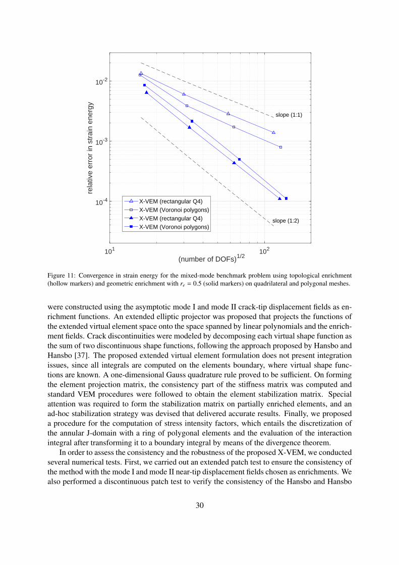
Figure 10 depicts convergence plots for the relative error in strain energy on quadrilateral andpolygonal meshes for the X-VEM with geometric enrichment. The convergence rate is closeto 2, which is consistent with theory. To provide a clearer picture, Fig. 11 shows a comparisonbetween the convergence plots in strain energy for both quadrilateral and polygonal meshes.
In order to assess the robustness and the accuracy of the X-VEM in providing stress inten-sity factors, we apply the procedure described in Section 4.4 to the problem at hand. For thisexample, the exact mode I and mode II stress intensity factors are KI = 1 and KII = 1. Both
27
101 102
(number of DOFs)1/2
10-4
10-3
10-2
10-1
rela
tive
erro
r in
str
ain
ener
gy
VEM (rectangular Q4)VEM (Voronoi polygons)X-VEM (rectangular Q4)X-VEM (Voronoi polygons)
slope (1:1)
Figure 9: Convergence in strain energy for the mixed-mode benchmark problem. For the X-VEM, only the node atthe origin is enriched (topological enrichment). Comparisons are shown with the standard VEM on quadrilateraland polygonal meshes. All methods converge with a rate close to unity.
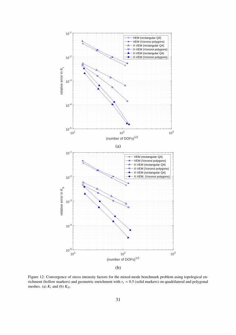
topological and geometric enrichment are considered. Stress intensity factors are computedconsidering a ring of elements placed at a radius rd = 0.4 from the origin.
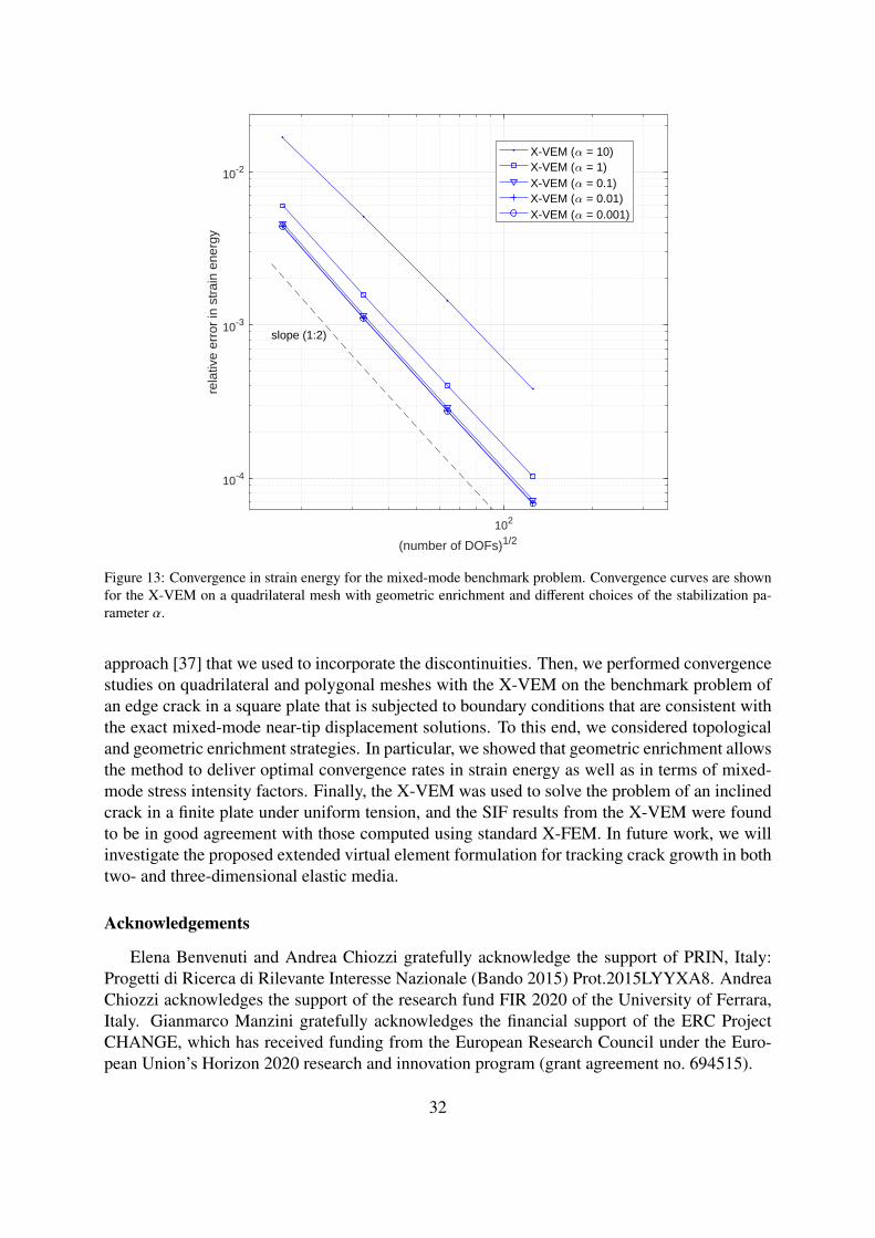
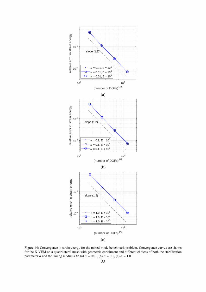
Figures 12a and 12b show the convergence of KI and KII on quadrilateral and polygonalmeshes. Convergence is stable on all the meshes and accuracy is sound. In particular, geo-metric enrichment enhances both the convergence rate and the accuracy. Finally, in Fig. 13 weinvestigate the influence of the scaling parameter α in the stabilization. Convergence is optimalfor α ranging from 10−3 to 10, with trends in improved accuracy towards smaller values of α.Moreover, as shown in Fig. 14, α does not need to be adjusted if the Young modulus E is varied:for a given α, the accuracy of the method is not significantly influenced by varying E.
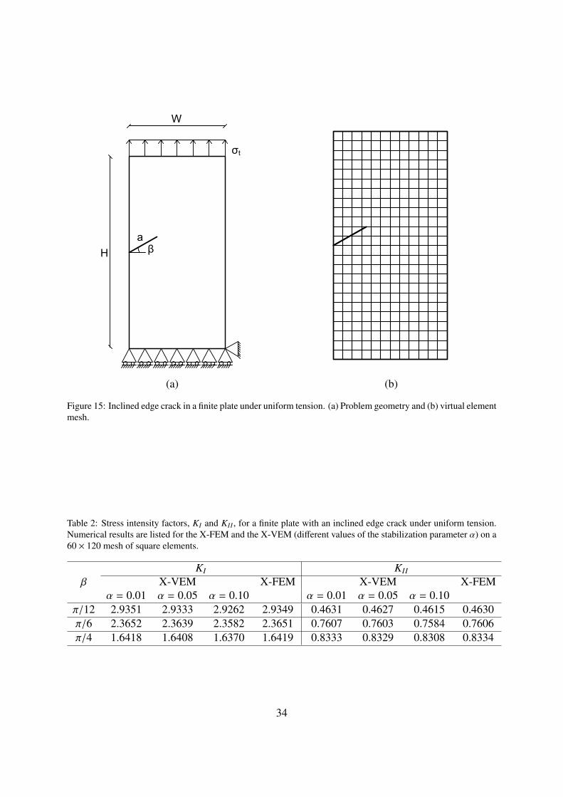
5.4. Inclined edge crack in a finite plate under uniform tensionWe now study the problem of an inclinded edge crack in a finite plate under uniform tension.
The geometry and boundary conditions are shown in Fig. 15. The plate width W = 6 and plateheight H = 3 are chosen. The crack has length a = 1 and is inclined at an angle β. Uniformtractions σt = 1 are applied on the top edge and horizontal rollers are imposed on the bottomedge. The exact solution for this problem in the neighborhood of the crack tip is given by alinear combination of the fields (14). However, the exact solution on the whole domain is notknown in closed-form.
Figures 16a and 16b show the convergence plots (inclination angles, β = 0 and β = π/6) in
28

101 102
(number of DOFs)1/2
10-5
10-4
10-3
10-2
10-1
rela
tive
erro
r in
str
ain
ener
gy
VEM (rectangular Q4)VEM (Voronoi polygons)X-VEM (rectangular Q4)X-VEM (Voronoi polygons)
slope (1:2)
Figure 10: Convergence in strain energy for the mixed-mode benchmark problem. For the X-VEM, geometricenrichment (re = 0.5) on quadrilateral and polygonal meshes is used. Comparisons are made with the standardVEM. X-VEM converges with a rate close to two.
terms of the relative error in strain energy on quadrilateral and polygonal meshes. The stabi-lization parameter α = 0.01 is chosen. Reference solution for the energy is computed with anoverkill mesh of 460.800 elements using the X-FEM. We use meshes of square elements withh = 1/4, 1/10, 1/20, 1/40, as well as polygonal (Voronoi) meshes. Convergence of the X-VEMis compared to standard VEM and X-FEM. The X-VEM displays sound accuracy for both meshtypes, and is comparable to that obtained with the X-FEM. Finally, in Fig. 17, convergence of KI
for β = π/6 is presented for different types of meshes and enrichment radii. Again, the obtainedresults are in good agreement with the X-FEM, which can be inferred from Table 2, where thenumerical results for KI and KII are listed for the X-FEM and for the X-VEM with differentvalues of the stabilization parameter α. As already noted in Section 5.3, here too smaller valuesof α improve the accuracy of the X-VEM.
6. Concluding remarks
We developed a stable and convergent extended virtual element method for two-dimensionalelastic fracture problems, which permits the incorporation of crack-tip singularities and discon-tinuities in the approximation space. Inspired by the construction of the X-FEM [3], we aug-mented the standard virtual element space by means of additional vectorial basis functions that
29
101 102
(number of DOFs)1/2
10-4
10-3
10-2
rela
tive
erro
r in
str
ain
ener
gy
X-VEM (rectangular Q4)X-VEM (Voronoi polygons)X-VEM (rectangular Q4)X-VEM (Voronoi polygons)
slope (1:2)
slope (1:1)
Figure 11: Convergence in strain energy for the mixed-mode benchmark problem using topological enrichment(hollow markers) and geometric enrichment with re = 0.5 (solid markers) on quadrilateral and polygonal meshes.
were constructed using the asymptotic mode I and mode II crack-tip displacement fields as en-richment functions. An extended elliptic projector was proposed that projects the functions ofthe extended virtual element space onto the space spanned by linear polynomials and the enrich-ment fields. Crack discontinuities were modeled by decomposing each virtual shape function asthe sum of two discontinuous shape functions, following the approach proposed by Hansbo andHansbo [37]. The proposed extended virtual element formulation does not present integrationissues, since all integrals are computed on the elements boundary, where virtual shape func-tions are known. A one-dimensional Gauss quadrature rule proved to be sufficient. On formingthe element projection matrix, the consistency part of the stiffness matrix was computed andstandard VEM procedures were followed to obtain the element stabilization matrix. Specialattention was required to form the stabilization matrix on partially enriched elements, and anad-hoc stabilization strategy was devised that delivered accurate results. Finally, we proposeda procedure for the computation of stress intensity factors, which entails the discretization ofthe annular J-domain with a ring of polygonal elements and the evaluation of the interactionintegral after transforming it to a boundary integral by means of the divergence theorem.
In order to assess the consistency and the robustness of the proposed X-VEM, we conductedseveral numerical tests. First, we carried out an extended patch test to ensure the consistency ofthe method with the mode I and mode II near-tip displacement fields chosen as enrichments. Wealso performed a discontinuous patch test to verify the consistency of the Hansbo and Hansbo
30
101 102 103
(number of DOFs)1/2
10-5
10-4
10-3
10-2
10-1
rela
tive
erro
r in
KI
VEM (rectangular Q4)VEM (Voronoi polygons)X-VEM (rectangular Q4)X-VEM (Voronoi polygons)X-VEM (rectangular Q4)X-VEM (Voronoi polygons)
(a)
101 102 103
(number of DOFs)1/2
10-5
10-4
10-3
10-2
10-1
rela
tive
erro
r in
KII
VEM (rectangular Q4)VEM (Voronoi polygons)X-VEM (rectangular Q4)X-VEM (Voronoi polygons)X-VEM (rectangular Q4)X-VEM, (Voronoi polygons)
(b)
Figure 12: Convergence of stress intensity factors for the mixed-mode benchmark problem using topological en-richment (hollow markers) and geometric enrichment with re = 0.5 (solid markers) on quadrilateral and polygonalmeshes. (a) KI and (b) KII .
31
102
(number of DOFs)1/2
10-4
10-3
10-2
rela
tive
erro
r in
str
ain
ener
gy
X-VEM ( = 10)X-VEM ( = 1)X-VEM ( = 0.1)X-VEM ( = 0.01)X-VEM ( = 0.001)
slope (1:2)
Figure 13: Convergence in strain energy for the mixed-mode benchmark problem. Convergence curves are shownfor the X-VEM on a quadrilateral mesh with geometric enrichment and different choices of the stabilization pa-rameter α.
approach [37] that we used to incorporate the discontinuities. Then, we performed convergencestudies on quadrilateral and polygonal meshes with the X-VEM on the benchmark problem ofan edge crack in a square plate that is subjected to boundary conditions that are consistent withthe exact mixed-mode near-tip displacement solutions. To this end, we considered topologicaland geometric enrichment strategies. In particular, we showed that geometric enrichment allowsthe method to deliver optimal convergence rates in strain energy as well as in terms of mixed-mode stress intensity factors. Finally, the X-VEM was used to solve the problem of an inclinedcrack in a finite plate under uniform tension, and the SIF results from the X-VEM were foundto be in good agreement with those computed using standard X-FEM. In future work, we willinvestigate the proposed extended virtual element formulation for tracking crack growth in bothtwo- and three-dimensional elastic media.
Acknowledgements
Elena Benvenuti and Andrea Chiozzi gratefully acknowledge the support of PRIN, Italy:Progetti di Ricerca di Rilevante Interesse Nazionale (Bando 2015) Prot.2015LYYXA8. AndreaChiozzi acknowledges the support of the research fund FIR 2020 of the University of Ferrara,Italy. Gianmarco Manzini gratefully acknowledges the financial support of the ERC ProjectCHANGE, which has received funding from the European Research Council under the Euro-pean Union’s Horizon 2020 research and innovation program (grant agreement no. 694515).
32
101 102
(number of DOFs)1/2
10-4
10-3
rela
tive
erro
r in
str
ain
ener
gy = 0.01, E = 105
= 0.01, E = 104
= 0.01, E = 103
slope (1:2)
(a)
101 102
(number of DOFs)1/2
10-4
10-3
rela
tive
erro
r in
str
ain
ener
gy
= 0.1, E = 105
= 0.1, E = 104
= 0.1, E = 103
slope (1:2)
(b)
101 102
(number of DOFs)1/2
10-4
10-3
rela
tive
erro
r in
str
ain
ener
gy
= 1.0, E = 105
= 1.0, E = 104
= 1.0, E = 103
slope (1:2)
(c)
Figure 14: Convergence in strain energy for the mixed-mode benchmark problem. Convergence curves are shownfor the X-VEM on a quadrilateral mesh with geometric enrichment and different choices of both the stabilizationparameter α and the Young modulus E: (a) α = 0.01, (b) α = 0.1, (c) α = 1.0
33
W
Haβ
σt
(a) (b)
Figure 15: Inclined edge crack in a finite plate under uniform tension. (a) Problem geometry and (b) virtual elementmesh.
Table 2: Stress intensity factors, KI and KII , for a finite plate with an inclined edge crack under uniform tension.Numerical results are listed for the X-FEM and the X-VEM (different values of the stabilization parameter α) on a60 × 120 mesh of square elements.
KI KII
β X-VEM X-FEM X-VEM X-FEMα = 0.01 α = 0.05 α = 0.10 α = 0.01 α = 0.05 α = 0.10
π/12 2.9351 2.9333 2.9262 2.9349 0.4631 0.4627 0.4615 0.4630π/6 2.3652 2.3639 2.3582 2.3651 0.7607 0.7603 0.7584 0.7606π/4 1.6418 1.6408 1.6370 1.6419 0.8333 0.8329 0.8308 0.8334
34
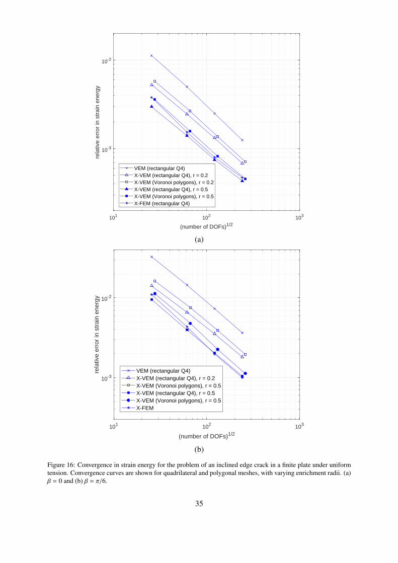
101 102 103
(number of DOFs)1/2
10-3
10-2
rela
tive
erro
r in
str
ain
ener
gy
VEM (rectangular Q4)X-VEM (rectangular Q4), r = 0.2X-VEM (Voronoi polygons), r = 0.2X-VEM (rectangular Q4), r = 0.5X-VEM (Voronoi polygons), r = 0.5X-FEM (rectangular Q4)
(a)
101 102 103
(number of DOFs)1/2
10-3
10-2
rela
tive
erro
r in
str
ain
ener
gy
VEM (rectangular Q4)X-VEM (rectangular Q4), r = 0.2X-VEM (Voronoi polygons), r = 0.5X-VEM (rectangular Q4), r = 0.5X-VEM (Voronoi polygons), r = 0.5X-FEM
(b)
Figure 16: Convergence in strain energy for the problem of an inclined edge crack in a finite plate under uniformtension. Convergence curves are shown for quadrilateral and polygonal meshes, with varying enrichment radii. (a)β = 0 and (b) β = π/6.
35
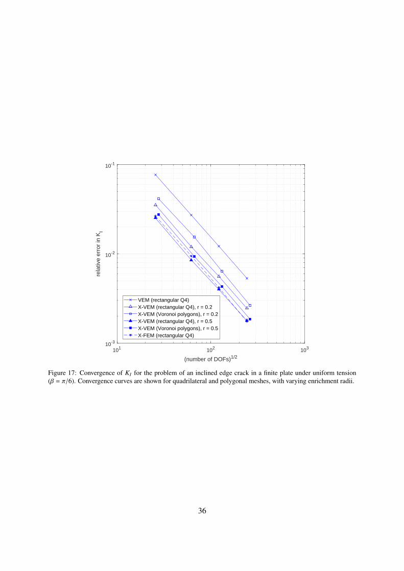
101 102 103
(number of DOFs)1/2
10-3
10-2
10-1
rela
tive
erro
r in
KI
VEM (rectangular Q4)X-VEM (rectangular Q4), r = 0.2X-VEM (Voronoi polygons), r = 0.2X-VEM (rectangular Q4), r = 0.5X-VEM (Voronoi polygons), r = 0.5X-FEM (rectangular Q4)
Figure 17: Convergence of KI for the problem of an inclined edge crack in a finite plate under uniform tension(β = π/6). Convergence curves are shown for quadrilateral and polygonal meshes, with varying enrichment radii.
36
References
[1] J. M. Melenk and I. Babuska. The partition of unity finite element method: Basic theoryand applications. Computer Methods in Applied Mechanics and Engineering, 139:289–314, 1996.
[2] I. Babuska and J. M. Melenk. The partition of unity method. International Journal forNumerical Methods in Engineering, 40:727–758, 1997.
[3] N. Moes, J. Dolbow, and T. Belytschko. A finite element method for crack growth withoutremeshing. International Journal for Numerical Methods in Engineering, 46(1):131–150,1999.
[4] A. Tabarraei and N. Sukumar. Extended finite element method on polygonal and quadtreemeshes. Computer Methods in Applied Mechanics and Engineering, 197(5):425–438,2008.
[5] A. Zamani and M. R. Eslami. Embedded interfaces by polytope FEM. InternationalJournal for Numerical Methods in Engineering, 88:715–748, 2011.
[6] C. Song and J. P. Wolf. The scaled boundary finite-element method – alias consistent in-finitesimal finite-element cell method – for elastodynamics. Computer Methods in AppliedMechanics and Engineering, 147:329–355, 1997.
[7] C. Song and J. P. Wolf. Semi-analytical representation of stress singularity as occurringin cracks in anisotropic multi-materials with the scaled boundary finite-element method.Computer and Structures, 80:183–197, 2002.
[8] C. Song, E. T. Ooi, and S. Natarajan. A review of the scaled boundary finite elementmethod for two-dimensional linear elastic fracture mechanics. Engineering Fracture Me-chanics, 187:45–73, 2018.
[9] S. E. Mousavi and N. Sukumar. Generalized Duffy transformation for integrating vertexsingularities. Computational Mechanics, 45(2–3):127–140, 2010.
[10] E. B. Chin, J. B. Lasserre, and N. Sukumar. Numerical integration of homogeneousfunctions on convex and nonconvex polygons and polyhedra. Computational Mechan-ics, 56(6):967–981, 2015.
[11] E. B. Chin, J. B. Lasserre, and N. Sukumar. Modeling crack discontinuities withoutelement-partitioning in the extended finite element method. International Journal forNumerical Methods in Engineering, 86(11):1021–1048, 2017.
[12] L. Beirao da Veiga, F. Brezzi, A. Cangiani, G. Manzini, L. D. Marini, and A. Russo.Basic principles of virtual element methods. Mathematical Models & Methods in AppliedSciences, 23:119–214, 2013.
[13] K. Lipnikov, G. Manzini, and M. Shashkov. Mimetic finite difference method. Journal ofComputational Physics, 257(Part B.):1163–1227, 2014.
37
[14] L. Beirao da Veiga, K. Lipnikov, and G. Manzini. The Mimetic Finite Difference Method,volume 11 of MS&A. Modeling, Simulations and Applications. Springer, I edition, 2014.
[15] L. Beirao da Veiga, F. Brezzi, and D. Marini. Virtual elements for linear elasticity prob-lems. SIAM Journal on Numerical Analysis, 51(2):794–812, 2013.
[16] A. L. Gain, C. Talischi, and G. H. Paulino. On the virtual element method for three-dimensional linear elasticity problems on arbitrary polyhedral meshes. Computer Methodsin Applied Mechanics and Engineering, 282:132–160, 2014.
[17] H. Chi, L. Beirao da Veiga, and G. H. Paulino. Some basic formulations of the virtualelement method (vem) for finite deformations. Computer Methods in Applied Mechanicsand Engineering, 318:142–190, 2017.
[18] P. Wriggers, B. D. Reddy, W. T. Rust, and B. Hudobivnik. Efficient virtual element for-mulations for compressible and incompressible finite deformations. Computational Me-chanics, 60:253–268, 2017.
[19] K. Park, H. Chi, and G.H. Paulino. B-bar virtual element method for nearly incompressibleand compressible materials. Meccanica, 56:1423—-1439, 2012.
[20] L. Beirao da Veiga, C. Lovadina, and D. Mora. A virtual element method for elastic andinelastic problems on polytope meshes. Computer Methods in Applied Mechanics andEngineering, 295:327–346, 2015.
[21] B. Hudobivnik, F. Aldakheel, and P. Wriggers. A low order 3d virtual element formulationfor finite elasto–plastic deformations. Computational Mechanics, 63:253—-269, 2019.
[22] E. Artioli, S. De Miranda, C. Lovadina, and L. Patruno. A stress/displacement virtualelement method for plane elasticity problems. Computer Methods in Applied Mechanicsand Engineering, 325:155–174, 2017.
[23] F. Dassi, C. Lovadina, and M. Visinoni. A three-dimensional Hellinger–Reissner virtualelement method for linear elasticity problems. Computer Methods in Applied Mechanicsand Engineering, 364:112910, 2020.
[24] E. Artioli, L. Beirao da Veiga, and F. Dassi. Curvilinear virtual elements for 2d solidmechanics applications. Computer Methods in Applied Mechanics and Engineering,359:112667, 2020.
[25] K. Park, H. Chi, and Paulino G.H. On nonconvex meshes for elastodynamics using vir-tual element methods with explicit time integration. International Journal for NumericalMethods in Engineering, 356:669–684, 2019.
[26] K. Park, H. Chi, and Paulino G.H. Numerical recipes for elastodynamic virtual elementmethods with explicit time integration. International Journal for Numerical Methods inEngineering, 121:1–31, 2020.
38
[27] P. F. Antonietti, G. Manzini, I. Mazzieri, H. M. Mourad, and M. Verani. The arbitrary-order virtual element method for linear elastodynamics models: convergence, stabilityand dispersion-dissipation analysis. International Journal for Numerical Methods in En-gineering, 122:934–971, 2021.
[28] M. F. Benedetto, S. Berrone, S. Pieraccini, and S. Scialo. The virtual element methodfor discrete fracture network simulations. Computer Methods in Applied Mechanics andEngineering, 280:135 – 156, 2014.
[29] V. M. Nguyen-Thanh, X. Zhuang, H. Ngyyen-Xuan, T. Rabczuk, and P. Wriggers. AVirtual Element Method for 2D linear elastic fracture analysis. Computer Methods inApplied Mechanics and Engineering, 340:366–395, 2018.
[30] A. Hussein, F. Aldakheel, B. Hudobivnik, P. Wrigger, P.A. Guidault, and O. Allix. Acomputational framework for brittle crack-propagation based on efficient virtual elementmethod. Computer Methods in Applied Mechanics and Engineering, 159:15–32, 2019.
[31] E. Artioli, S. Marfia, and E. Sacco. VEM-based tracking algorithm for cohesive/frictional2d fracture. Computer Methods in Applied Mechanics and Engineering, 365:112956,2020.
[32] I. Perugia, P. Pietra, and A. Russo. A plane wave virtual element method for the Helmholtzproblem. ESAIM: Mathematical Modelling and Numerical Analysis, 50(3):783–808,2016.
[33] E. Benvenuti, A. Chiozzi, G. Manzini, and N. Sukumar. Extended virtual element methodfor the Laplace problem with singularities and discontinuities. Computer Methods in Ap-plied Mechanics and Engineering, 356:571–597, 2019.
[34] A. Chiozzi and E. Benvenuti. Extended virtual element method for the torsion problem ofcracked prismatic beams. Meccanica, 55:637–648, 2020.
[35] E. Artioli and L. Mascotto. Enrichment of the nonconforming virtual element methodwith singular functions. Computer Methods in Applied Mechanics and Engineering,385:114024, 2021.
[36] C. A. Duarte, I. Babuska, and J. T. Oden. Generalized finite element methods for three-dimensional structural mechanics problems. Computer and Structures, 77:215–232, 2000.
[37] A. Hansbo and P. Hansbo. A finite element method for the simulation of strong andweak discontinuities in solid mechanics. Computer Methods in Applied Mechanics andEngineering, 193(33-35):3523–3540, 2004.
[38] P. Grisvard. Singularities in Boundary Value Problems. Masson, Paris, France, 1992.
[39] P. M. A. Areias and T. Belytschko. A comment on the article ‘A finite element methodfor simulation of strong and weak discontinuities in solid mechanics’ by A. Hansbo andP. Hansbo [Comput. Methods Appl. Mech. Engrg. 193 (2004) 3523-3540]. ComputerMethods in Applied Mechanics and Engineering, 195:1275–1276, 2006.
39
[40] J. Duchon. Splines minimizing rotation-invariant semi-norms in Sobolev spaces. In Con-structive Theory of Functions of Several Variables, volume 571 of Lecture Notes in Math-ematics, pages 85–100. Springer-Verlag, Berlin, Germany, 1977.
[41] E. Benvenuti and N. Orlando. A mesh-independent framework for crack tracking in elas-todamaging materials through the regularized extended finite element method. Computa-tional Mechanics, 68:25–49, 2021.
[42] L. Beirao da Veiga, F. Brezzi, L. D. Marini, and A. Russo. The hitchhiker’s guide to the vir-tual element method. Mathematical Models & Methods in Applied Sciences, 24(8):1541–1573, 2014.
[43] L. Beirao da Veiga, F. Dassi, and A. Russo. High-order virtual element method on poly-hedral meshes. Computers and Mathematics with Applications, 74:1110–1122, 2017.
[44] J. Rice. A path independent integral and the approximate analysis of strain concentrationby notches and cracks. Journal of Applied Mechanics, 35:379–386, 1968.
[45] F. Z. Li, C. F. Shih, and A. Needleman. A comparison of methods for calculating energyrelease rates. Engineering Fracture Mechanics, 21(2):405–421, 1985.
[46] L. Beirao da Veiga, A. Chernov, L. Mascotto, and A. Russo. Exponential convergence ofthe hp virtual element method in presence of corner singularities. Numerische Mathematik,138:581–613, 2018.
[47] J. E. Dolbow and A. Devan. Enrichment of enhanced assumed strain approximationsfor representing strong discontinuities: addressing volumetric incompressibility and thediscontinuous patch test. International Journal for Numerical Methods in Engineering,59(1):47–67, 2004.
[48] C. Talischi, G. H. Paulino, A. Pereira, and F. M. Menezes. PolyMesher: a general-purposemesh generator for polygonal elements written in Matlab. Structural and MultidisciplinaryOptimization, 45(3):309–328, 2012.
[49] P. Grisvard. Elliptic Problems in Nonsmooth Domains. Pitman Publishing, Inc, Boston,MA, 1985.
[50] P. Laborde, J. Pommier, Y. Renard, and M. Salaun. High-order extended finite elementmethod for cracked domains. International Journal for Numerical Methods in Engineer-ing, 64(3):354–381, 2005.
[51] E. Bechet, H. Minnebo, N. Moes, and B. Burgardt. Improved implementation and ro-bustness study of the X-FEM for stress analysis around cracks. International Journal forNumerical Methods in Engineering, 64(8):1033–1056, 2005.
40


![Bone Tissue Mechanics - FenixEdu · Bone Tissue Mechanics João Folgado ... Introduction to linear elastic fracture mechanics ... Lesson_2016.03.14.ppt [Compatibility Mode]](https://img.pdfslide.tips/doc/110x75/5ae984637f8b9aee0790eb6e/bone-tissue-mechanics-tissue-mechanics-joo-folgado-introduction-to-linear.jpg)