Embed Size (px)
Citation preview
Fakultat fur Physik
Fundamental physics with neutrons
Electric dipole moment searches
using the isotope 129-xenon
Florian Kuchler
Vollstandiger Abdruck der von der Fakultat fur Physik der Technischen UniversitatMunchen zur Erlangung des akademischen Grades eines
Doktors der Naturwissenschaften (Dr. rer. nat.)
genehmigten Dissertation.
Vorsitzende: Univ.-Prof. Dr. Nora Brambilla
Prufer der Dissertation:
1. Univ.-Prof. Dr. Peter Fierlinger2. Univ.-Prof. Dr. Elisa Resconi
Die Dissertation wurde am 03.11.2014 bei der Technischen Universitat Munchen eingere-icht und durch die Fakultat fur Physik am 13.11.2014 angenommen.

Abstract
The search for permanent electric dipole moments (EDM) of fundamental systems ismotivated by their time-reversal and parity violating nature. A non-zero EDM impliesa new source of CP violation, essential to explain the huge excess of matter over anti-matter in our Universe. Moreover, an EDM is a clean probe of physics beyond theStandard Model (SM).Besides other fundamental systems the diamagnetic atom 129Xe is a particularly interest-ing candidate for an EDM search due to its unique properties. Considering semileptonicCP violating interactions, 129Xe offers a higher sensitivity compared to 199Hg when mea-sured at the same level. Also, adding a new limit of the EDM of 129Xe to superior resultfrom 199Hg can significantly improve existing constraints on hadronic CP odd couplings.In this work two new complementary EDM experiments are discussed, which both intro-duce highly sensitive SQUID detection systems, but feature totally different systematics.A novel approach is based on sub-millimeter hyper-polarized liquid xenon droplets en-closed on a micro-fabricated structure. Implementation of rotating electric fields en-ables a conceptually new EDM measurement technique, potentially overcoming currentsensitivity limitations while allowing thorough investigation of new systematic effects.However, an established “Ramsey-type” spin precession experiment with static electricfield can be realized at similar sensitivity within the same setup. Employing supercon-ducting pick-up coils and highly sensitive LTc-SQUIDs, a large array of independentmeasurements can be performed simultaneously with different configurations. With thisnew approach we aim to finally lower the limit on the EDM of 129Xe by about threeorders of magnitude. The method and new systematic effects are discussed limiting thisapproach to about 10−30 ecm. Operation of superconducting pickup coils mounted closeto a high temperature sample in a cryogen-free environment as well as production andtransport of polarized xenon is demonstrated.In the second experiment a 3He co-magnetometer is introduced in a newly developedEDM cell with silicon electrodes. Here, established techniques with well known system-atics are improved and the experiment placed in a magnetically shielded environment,particularly developed for low energy precession experiments. Under these nearly per-fect conditions and with high signal-to-noise ratio due to SQUID detection, it is demon-strated, that first successful measurements with applied high voltage yield competitiveEDM sensitivity.The two experiments feature different systematics and represent a balance between mod-erate short-term improvements and a long-term high gain in sensitivity involving exten-sive R&D work.
iii

Contents
1 Introduction 1
2 Electric dipole moment (EDM): Motivation, theory and experiments 3
2.1 The matter-antimatter mystery . . . . . . . . . . . . . . . . . . . . . . . . 3
2.2 Baryon asymmetry and CP violation in the Standard Model (SM) . . . . 4
2.3 Permanent electric dipole moments as probes of CP violation . . . . . . . 6
2.4 Mechanisms generating EDMs of atoms . . . . . . . . . . . . . . . . . . . 7
2.4.1 T, P odd nuclear moments . . . . . . . . . . . . . . . . . . . . . . 8
2.4.2 Electron-nucleon interaction . . . . . . . . . . . . . . . . . . . . . . 11
2.4.3 Electron EDM . . . . . . . . . . . . . . . . . . . . . . . . . . . . . 12
2.5 Sensitivity of EDMs to physics beyond the SM . . . . . . . . . . . . . . . 13
2.6 Experimental status and prospects of EDM searches . . . . . . . . . . . . 17
3 Optimizing the parameter space for a new 129Xe EDM search 21
3.1 Atomic physics . . . . . . . . . . . . . . . . . . . . . . . . . . . . . . . . . 21
3.1.1 Atomic magnetic moments and level splitting . . . . . . . . . . . . 21
3.1.2 Nuclear magnetic resonance . . . . . . . . . . . . . . . . . . . . . . 23
3.1.3 Time-varying magnetic fields . . . . . . . . . . . . . . . . . . . . . 25
3.2 Spin exchange optical pumping of 129Xe and 3He . . . . . . . . . . . . . . 25
3.2.1 Optical pumping of alkali metals . . . . . . . . . . . . . . . . . . . 26
3.2.2 Alkali-noble gas collisions . . . . . . . . . . . . . . . . . . . . . . . 29
3.3 Relaxation mechanisms of polarized 129Xe and 3He . . . . . . . . . . . . 32
3.3.1 Gas phase relaxation of 129Xe and 3He . . . . . . . . . . . . . . . 33
3.3.2 Solid phase relaxation of 129Xe . . . . . . . . . . . . . . . . . . . . 37
3.3.3 Liquid phase relaxation of 129Xe . . . . . . . . . . . . . . . . . . . 40
3.4 SQUID detection . . . . . . . . . . . . . . . . . . . . . . . . . . . . . . . . 42
3.4.1 Superconductivity and the Josephson effect . . . . . . . . . . . . . 42
3.4.2 SQUIDs and the flux-locked loop . . . . . . . . . . . . . . . . . . . 43
3.4.3 Practical SQUID magnetometers and gradiometers . . . . . . . . . 47
4 Improving EDM measurements of 129Xe 49
4.1 Background . . . . . . . . . . . . . . . . . . . . . . . . . . . . . . . . . . . 49
4.2 Fundamental limitations . . . . . . . . . . . . . . . . . . . . . . . . . . . . 51
4.2.1 Methods to improve EDM sensitivity . . . . . . . . . . . . . . . . . 51
4.2.2 An improved conventional EDM search . . . . . . . . . . . . . . . 52
4.2.3 Next generation EDM search in liquid 129Xe . . . . . . . . . . . . 53
v
Contents
5 Progress towards a liquid 129Xe EDM experiment 555.1 A novel approach to measure the EDM of 129Xe . . . . . . . . . . . . . . . 57
5.1.1 Different ways to search for an EDM within this approach . . . . . 575.1.2 Experimental realization . . . . . . . . . . . . . . . . . . . . . . . . 595.1.3 New systematic effects due to rotating electric fields . . . . . . . . 615.1.4 Conclusion . . . . . . . . . . . . . . . . . . . . . . . . . . . . . . . 67
5.2 A cryogen-free SQUID cryostat with variable sample temperature . . . . . 695.2.1 Introduction . . . . . . . . . . . . . . . . . . . . . . . . . . . . . . 695.2.2 Apparatus . . . . . . . . . . . . . . . . . . . . . . . . . . . . . . . . 705.2.3 Measurements . . . . . . . . . . . . . . . . . . . . . . . . . . . . . 755.2.4 Conclusion and outlook . . . . . . . . . . . . . . . . . . . . . . . . 79
5.3 Pickup coils and SQUID signal calibration . . . . . . . . . . . . . . . . . . 805.4 Xenon polarizing setup . . . . . . . . . . . . . . . . . . . . . . . . . . . . . 815.5 Accumulation and transfer of polarized xenon . . . . . . . . . . . . . . . . 855.6 Generation and shielding of magnetic fields . . . . . . . . . . . . . . . . . 875.7 Development of the “EDM chip” . . . . . . . . . . . . . . . . . . . . . . . 905.8 Summary of the liquid xenon EDM experiment . . . . . . . . . . . . . . . 92
6 A new EDM experiment using a He/Xe mixture and SQUID detection 956.1 The SQUID system and polarization setup . . . . . . . . . . . . . . . . . . 976.2 Progress and test measurement results . . . . . . . . . . . . . . . . . . . . 99
6.2.1 A first spin-precession signal of 129Xe . . . . . . . . . . . . . . . . 1006.2.2 Spin-flip sequence on highly polarized 3He . . . . . . . . . . . . . 1026.2.3 Spin-precession of both species in an electric field . . . . . . . . . . 1056.2.4 Potential of the magnetic shielding insert . . . . . . . . . . . . . . 112
6.3 Summary of the He/Xe EDM search . . . . . . . . . . . . . . . . . . . . . 112
7 Conclusion and outlook 1137.1 Progress towards a liquid 129Xe EDM experiment . . . . . . . . . . . . . . 1137.2 Status of the clock-comparison 129Xe EDM search . . . . . . . . . . . . . 115
A Appendix 117A.1 Analytical expressions of nuclear moments . . . . . . . . . . . . . . . . . . 117A.2 The relations of electron-nucleon coupling coefficients . . . . . . . . . . . . 118A.3 A limit on the electon EDM from diamagnetic atoms . . . . . . . . . . . . 118A.4 Diffusion in multi-component gas mixtures . . . . . . . . . . . . . . . . . . 119A.5 Properties of relevant atoms . . . . . . . . . . . . . . . . . . . . . . . . . . 120A.6 Supplemental data . . . . . . . . . . . . . . . . . . . . . . . . . . . . . . . 121
A.6.1 Flexible circuits simulations . . . . . . . . . . . . . . . . . . . . . . 121A.6.2 EDM chip temperature difference . . . . . . . . . . . . . . . . . . . 121A.6.3 Rubidium vapor pressure . . . . . . . . . . . . . . . . . . . . . . . 122
vi
1 Introduction
Searches for electric dipole moments (EDM) are motivated by their symmetry-violatingnature. An EDM of a fundamental system is a manifestation of time-reversal violationand hence also breaks CP symmetry1. The violation of CP symmetry is essential toexplain the observed asymmetry of baryons to anti-baryons in the Universe. In the wellestablished Standard model of particle physics (SM), CP violation occurs only through(i) θ in quantum chromodynamics (QCD) and (ii) the complex phase δ in the CKMmatrix. Experiments strongly limit θ and determine δ very well. As a result only smallCP violation is generated in the SM, which is far from being sufficient to account forcosmological observations of the baryon number to photon ratio. This poses one of themost important fundamental puzzles in physics:
How did baryon asymmetry emerge from the early Universe?
Models extending the SM try to solve this question (and others). In particular, Su-persymmetry (SUSY) is very popular, but suffers from recent (non-)observations at theLarge Hadron Collider (LHC), where as of yet no supersymmetric partner particles werefound at the accessible energies. However, most extensions of the SM also require largerEDMs than the SM predicts. Hence, EDMs provide a probe for new physics and EDMsearches help constrain parameters of the new physics models. In this regard an ultra-low energy EDM search is complementary to extremely high energy experiments at LHC.
Besides fundamental systems like neutrons, diamagnetic atoms, particularly 129Xe and199Hg with nuclear spin 1/2, are interesting candidates for an EDM experiment. Thecurrent best limit on an EDM was obtained from 199Hg, with sensitivity improvementspublished in recent years. Despite the more complicated internal structure the 199HgEDM limit is widely used to constrain many new physics parameters as it has evenhigher sensitivity than more fundamental systems, e.g. the neutron. In the evolutionof new EDM limits, 129Xe has fallen behind recently, with the last published result in2001. However, the role of 129Xe is special in the sense that some of the fundamen-tal CP violating parameters can be better constrained by an (improved) EDM limit on129Xe, as I will point out in the first chapter, particularly in Sec. 2.6.
In this thesis I will introduce two new experiments at the TU Munchen searching for anEDM of the diamagnetic atom 129Xe in both gas and liquid phase using superconduct-ing quantum interference devices (SQUIDs) for signal detection. The usually employedmethod looking for deviations in spin-precession frequency in applied parallel magnetic
1The CP operator describes subsequent application of charge-conjugation C and the parity operator P .
1
1 Introduction
and electric fields in the gas phase seems to get closer to a dead-end in sensitivity. Toovercome these limitations, the development of new methods is highly motivated.The R&D efforts towards a liquid xenon EDM experiment are presented in Sec. 5. Itintroduces a completely new measurement method with time-varying electric fields. Thepotential sensitivity of the novel method and the resulting new systematic effects arediscussed in Sec. 5.1. In Sec. 5.2 the cryogenic setup for cooling and operating theSQUID sensors as well as details on the temperature control of the liquid xenon sampleare presented. In subsequent sections supplemental information on the main componentsfor production, accumulation and transfer of hyper-polarized xenon is given. The chap-ter concludes with remarks on the development of a micro-structured “EDM chip” inthe EDM cryostat,where polarized xenon is liquefied for the future EDM measurement.In summary the evaluation of new effects due to time-varying electric fields reveals sys-tematic uncertainties on a 10−30 ecm level suggesting a potential improvement on thexenon EDM limit by more than two orders of magnitude. However the novel systematicsof this approach have to be studied experimentally to quote reliable estimates. It is alsodemonstrated that the detection system of external superconducting pickup coils andSQUID current sensors can be operated in a cryogen-free setup at a magnetic flux noiselevel of 144 fT/
√Hz above 50Hz with a close-by sample at 162K. Along with success-
ful production and accumulation of hyper-polarized xenon a comprehensive area rich offurther physics studies for a high potential new xenon EDM search is now available fornew graduate students.
In contrast to the long-term development for this novel approach a new EDM experimentusing rather established well-known techniques is underway together with collaboratorsfrom the University of Michigan, Michigan State University, PTB Berlin and the Maier-Leibnitz Zentrum. This effort promises short-term results as a known “conventional”method is used basically improved by means of SQUID detection. At the TU Munchenthe best possible environment with lowest residual magnetic field and magnetic fieldgradients is available inside a state-of-the-art magnetically shielded room. By employ-ing highly sensitive SQUID detection we demonstrated the new concept to improve thecurrent EDM limit on xenon by at least an order of magnitude in the short-term.The current status and progress in this He-Xe spin-clock comparison approach is pre-sented in Sec. 6. The results of two test runs are discussed, including an already success-ful observation of simultaneous spin-precession of 3He and 129Xe in a prototype EDMcell with high voltage applied. The non-optimized EDM sensitivity of this measurementis already on the order of 10−23 ecm. With several straightforward improvements weanticipate a sensitivity of 10−26 ecm in a single run of 100 s.
The fast progress of the latter EDM search and the high potential gain of the noveltime-varying electric field approach make both EDM experiments very valuable for thesearch of new physics.
2
2 Electric dipole moment (EDM):Motivation, theory and experiments
2.1 The matter-antimatter mystery
In many aspects predictions according to the SM have been experimentally confirmedwith high precision. The signal of a Higgs-like particle measured at the LHC at a massof about 125 GeV has been found recently [1, 2] and provides another important successof the SM2.Nevertheless there are many open questions and shortcomings in the SM. Besides theunsolved nature of Dark Matter, Mass Hierarchy and other fundamental problems, theSM can not sufficiently account for the huge excess of matter over antimatter observedin our Universe.The strong matter-antimatter asymmetry in our local region up to the scale of galaxyclusters is evident from γ-ray observations and the absence of an excess of anti-particlesin cosmic rays. Also, there are arguments that rule out domains of large abundancesof antimatter on scales less than our visible Universe [3–5]. From precise measurementsof the Cosmic Microwave Background Radiation, the ratio of the difference of baryonand anti-baryon number densities nB = nb−nb to photon number density nγ in today’sUniverse is determined to [6, 7]
η =nBnγ
= 6.1+0.3−0.2 × 10⁻¹⁰. (2.1)
A similar value of η can be deduced from ratios of light element abundances from BigBang Nucleosynthesis [8]. As the present nB evolved from a difference in number densityof baryons and anti-baryons nb − nb in the early Universe, where at high temperaturesnb ≈ nb ≈ nγ , a tiny baryon excess of 1 part in 1010 led to all of the ordinary matter inthe Universe.Today’s baryon abundance predicted from symmetric cosmological models (with initiallynb = nb) is no where near the observed η ≈ 10−10. When in the early Universe the tem-perature was sufficiently high, a thermal equilibrium of annihilation and pair-productionof nucleons N and anti-nucleons N is maintained: N + N γ + γ. As the tempera-ture decreases fewer baryon-anti-baryon pairs are generated and annihilation processesN + N → γ + γ are favoured. With lower particle density annihilations cease and ef-fectively stop at a freeze-out temperature Tf ≈ 20MeV, when the expansion rate of the
2Although the nature the Higgs-like observation still has to be clarified. As yet the findings are consis-tent with a SM Higgs boson.
3
2 Electric dipole moment (EDM): Motivation, theory and experiments
Universe becomes larger than the annihilation rate. From the temperature dependenceof the baryon density to photon density one obtains at the freeze-out temperature [3, 9]
nbnγ
≈ 10−18, (2.2)
which is eight orders of magnitude smaller than the value determined from observations.
2.2 Baryon asymmetry and CP violation in the Standard
Model (SM)
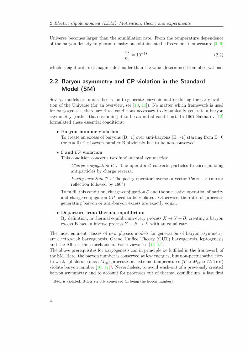
Several models are under discussion to generate baryonic matter during the early evolu-tion of the Universe (for an overview, see [10, 11]). No matter which framework is usedfor baryogenesis, there are three conditions necessary to dynamically generate a baryonasymmetry (rather than assuming it to be an initial condition). In 1967 Sakharov [12]formulated these essential conditions:
• Baryon number violation
To create an excess of baryons (B=1) over anti-baryons (B=-1) starting from B=0(or η = 0) the baryon number B obviously has to be non-conserved.
• C and CP violation
This condition concerns two fundamental symmetries:
Charge-conjugation C : The operator C converts particles to correspondingantiparticles by charge reversal
Parity operation P : The parity operator inverses a vector Px = −x (mirrorreflection followed by 180)
To fulfill this condition, charge-conjugation C and the successive operation of parityand charge-conjugation CP need to be violated. Otherwise, the rates of processesgenerating baryon or anti-baryon excess are exactly equal.
• Departure from thermal equilibrium
By definition, in thermal equilibrium every process X → Y +B, creating a baryonexcess B has an inverse process Y +B → X with an equal rate.
The most eminent classes of new physics models for generation of baryon asymmetryare electroweak baryogenesis, Grand Unified Theory (GUT) baryogenesis, leptogenesisand the Affleck-Dine mechanism. For reviews see [13–15].The above prerequisites for baryogenesis can in principle be fulfilled in the framework ofthe SM. Here, the baryon number is conserved at low energies, but non-perturbative elec-troweak sphaleron (mass Msp) processes at extreme temperatures (T ≈Msp ≈ 7.2TeV)violate baryon number [16, 17]3. Nevertheless, to avoid wash-out of a previously createdbaryon asymmetry and to account for processes out of thermal equilibrium, a fast first
3B+L is violated, B-L is strictly conserved (L being the lepton number)
4
2.2 Baryon asymmetry and CP violation in the Standard Model (SM)
order phase transition in the early Universe is essential. In the SM the electroweak phasetransition is not of first order and can thus not adequately describe baryogenesis. Atleast minimal extensions to the SM are necessary to resolve these issues.4
Regarding the second condition the SM also doesn’t provide sufficient CP violation.More detail on this particular issue will be given in the following as this is stronglyrelated to the search for EDMs, see Sec. 2.3.
Parity and charge-conjugation in the SMIn electromagnetic and strong interactions of the SM, parity is conserved. However,
parity violation in weak interactions was experimentally confirmed by Wu in 1957 [21]following a proposal from 1956 by Lee and Yang [22]. In Wu’s experiment the directionof emitted electrons in the weak decay 60Co → 60Ni∗ + e− + ν → 60Ni + 2γ + e− + νwas determined for the 60Co nuclear spin aligned both up and down. Surprisingly,they observed all electrons being emitted to the direction opposite to the nuclear spinorientation. This implies, that parity is not only violated but that parity symmetry ismaximally broken in weak interactions. This fact could be accounted for in the SM, byadding an axial vector ∝ ǫgwγ
5 to the Lagrangian of the weak interaction, with the weakcoupling constant gw and the Dirac matrix γ5. As parity is maximally violated in weakinteractions ǫ = −1.Charge conjugation is also strongly violated in the weak interaction, as only left-handedneutrinos and right-handed anti-neutrinos are observed.
CP violation in the weak sectorThe symmetry of the operator CP in the SM was assumed to hold [23], before Cronin
and Fitch observed CP violation in the weak decay of neutral kaons [24]. In a “pure”beam of a superposition state of the neutral kaon and it’s anti-particle two-pion de-cays on the order of 10−3 were observed, which are forbidden by CP symmetry. Later
CP violation was also found in the B0 B0system [25, 26].
Including this small effect of non-conservation of CP in the SM lead to the predictingof a third quark generation. Cabibbo’s [27] theory of mixing of two quark generations,described by a single (real) mixing angle (Cabbibo angle) was extended by Kobayashiet al. [28]. The parametrization of the resulting Cabibbo-Kobayashi-Maskawa (CKM)matrix now describes the quark mixing by three generalized Cabibbo angles θ12, θ23, θ13and a complex phase δ, which accounts for observed CP violation.
CP violation in the strong interactionIn QCD, CP violation is in principal possible via the θ-term in the SM Lagrangian.
But, the experimental limit on the EDM of the neutron already strongly constraints
4An extension of the SM actually has been found by the observation of neutrino oscillations [18–20],which confirm non-zero neutrino masses. This allows for a leptonic flavor mixing matrix required forbaryogenesis via leptogenesis. It is still under discussion whether the observed baryon asymmetrycan be accounted for by leptogenesis.
5
2 Electric dipole moment (EDM): Motivation, theory and experiments
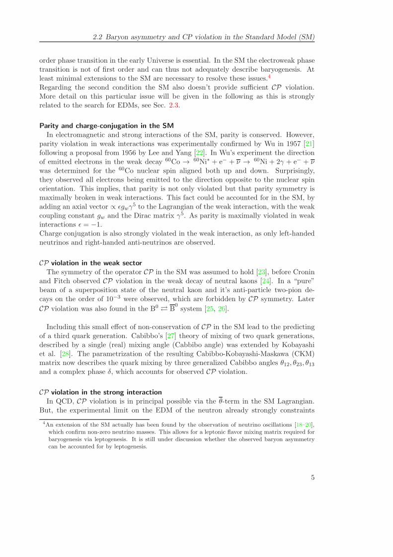
B S E B.S E.S
Parity +1 +1 -1 +1 -1
Time reversal -1 -1 +1 +1 -1 T
Pd
d
d µ
µ
µ
Fig. 1: Under the parity and time-reversal operation polar (electric field E) and axial (magneticfield B, spin S) vectors transform differently. Hence, a term dE.S in the Hamiltonian is parityand time-reversal violating, unless d = 0.
CP violation from the θ-term to be extremely small (cf. Sec. 2.5).
In summary, the SM - although being largely successful - can not provide sufficientmechanisms for B-violation, C and CP violation and processes out of thermal equilib-rium. Models beyond the SM, e.g. supersymmetric models, often provide mechanismsfor additional CP violation. Searching for observable properties generated by thesemechanisms is highly motivated to constrain model parameters.
2.3 Permanent electric dipole moments as probes of CP
violation
An unmistakable manifestation of CP violation is a permanent EDM of an elementarysystem. In this section I will introduce the properties of EDMs, mechanisms that gen-erate EDMs and discuss the sensitivity to new physics of various EDM measurements.Finally, the current status of EDM searches in different systems (neutrons, electrons andatoms) and perspectives of future improvements will be discussed.The T and P violating nature of an EDM can be understood by the different propertiesof transformations of axial and polar vectors under coordinate inversion and time rever-sal, see Fig. 1. Assuming CPT symmetry5 a non-zero EDM implies also CP violation.Moreover, the P odd property makes an EDM a very clean probe of new physics.
The Hamiltonian of a spin-12 particle with spin S, electric dipole moment d andmagnetic moment µ in both a magnetic field B and an electric field E
H = −µB.SS
− dE.S
S(2.3)
is only invariant under P and T for d = 0.EDMs are sensitive probes for new CP odd interactions as well as tests of T symmetry.A non-zero EDM would provide strong evidence for new physics beyond the SM. In thefollowing mechanisms generating EDMs from P and T symmetry violating mechanismswill be discussed.5This symmetry is expected to be valid, as violation of the CPT theorem has very profound conse-quences, like Lorentz invariance violation [29].
6
2.4 Mechanisms generating EDMs of atoms
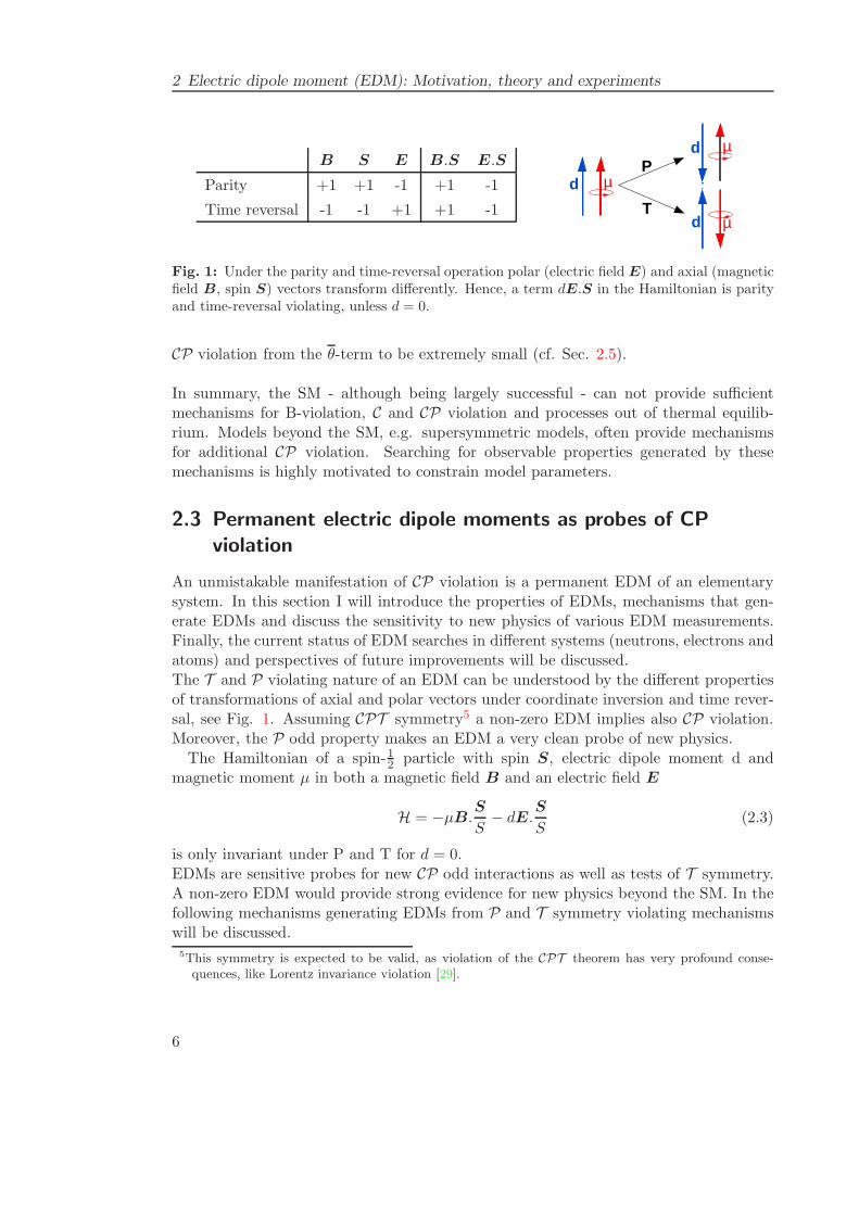
Fig. 2: Shown are sources contributing to EDMs of elementary particles dn, de, paramagneticatoms, molecules and diamagnetic atoms on different energy scales. To pin down underlyingdominant (solid) and higher order (dashed) contributions information from several fundamentalsystems is absolutely necessary.
2.4 Mechanisms generating EDMs of atoms
The physics underlying the generation of an observable EDM is currently not conclu-sively understood and the exact mechanisms need to be clarified by experiments. Nev-ertheless, for different fundamental systems like elementary particles, diamagnetic andparamagnetic atoms or molecules, the physics inducing EDMs can be categorized.
Fig. 2 shows an overview depicting the sources contributing to various systems. Refer-ences [30–33] give reviews on EDM inducing mechanisms focusing mostly on the neutronand atom EDMs. In the neutron as an elementary system sources of an EDM are intrin-sic EDMs of the constituent quarks dq and various interactions between quarks (qqqq),
quarks and gluons (the so called chromo-EDMs dq) or couplings of gluons (GG,GGG),where the two-gluon term leads to the famous θ term in QCD.
In more complex systems also electron interactions and an electron EDM contributesto the atomic EDM. The contributions to an atomic EDM at the nuclear level (<1 GeV)can be categorized as
• the intrinsic EDM of an electron de,
• the intrinsic EDM of a valence nucleon dn, dp.
• P ,T odd electron-nucleon interactions and
• P ,T odd nucleon-nucleon interactions.
As discussed in the following an EDM of diamagnetic atom mainly arises from anintrinsic nucleon EDM and T ,P odd nucleon-nucleon interactions. Effects on atomEDMs by an electron EDM and T ,P odd electron-nucleon interactions will also beadressed.Naively, an EDM of a nucleus is supposed to be screened by the electron cloud and
7
2 Electric dipole moment (EDM): Motivation, theory and experiments
hence is not observable6. This so called Schiff screening was shown to be complete fora quantum system of point-like electric dipoles in an external electric field of arbitraryshape by Schiff [34]. However, this so-called Schiff shielding is suppressed by relativisticeffects7 in paramagnetic atoms [35, 36] and finite size effects in diamagnetic atoms [34].In a simple picture the electric field is only canceled on average inside the nucleus,but not necessarily at the location of an unpaired valence nucleon. On an atomic levelthis effect can be deduced by a multipole expansion of the electrostatic potential of thenucleus.
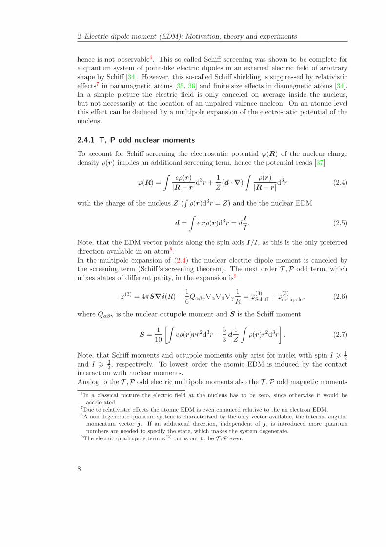
2.4.1 T, P odd nuclear moments
To account for Schiff screening the electrostatic potential ϕ(R) of the nuclear chargedensity ρ(r) implies an additional screening term, hence the potential reads [37]
ϕ(R) =
∫eρ(r)
|R− r|d3r +
1
Z(d ·∇)
∫ρ(r)
|R− r|d3r (2.4)
with the charge of the nucleus Z (∫ρ(r)d3r = Z) and the the nuclear EDM
d =
∫e rρ(r)d3r = d
I
I. (2.5)
Note, that the EDM vector points along the spin axis I/I, as this is the only preferreddirection available in an atom8.In the multipole expansion of (2.4) the nuclear electric dipole moment is canceled bythe screening term (Schiff’s screening theorem). The next order T ,P odd term, whichmixes states of different parity, in the expansion is9
ϕ(3) = 4πS∇δ(R) − 1
6Qαβγ∇α∇β∇γ
1
R= ϕ
(3)Schiff + ϕ
(3)octupole, (2.6)
where Qαβγ is the nuclear octupole moment and S is the Schiff moment
S =1
10
[∫eρ(r)rr2d3r − 5
3d1
Z
∫ρ(r)r2d3r
]. (2.7)
Note, that Schiff moments and octupole moments only arise for nuclei with spin I > 12
and I > 32 , respectively. To lowest order the atomic EDM is induced by the contact
interaction with nuclear moments.Analog to the T ,P odd electric multipole moments also the T ,P odd magnetic moments
6In a classical picture the electric field at the nucleus has to be zero, since otherwise it would beaccelerated.
7Due to relativistic effects the atomic EDM is even enhanced relative to the an electron EDM.8A non-degenerate quantum system is characterized by the only vector available, the internal angularmomentum vector j. If an additional direction, independent of j, is introduced more quantumnumbers are needed to specify the state, which makes the system degenerate.
9The electric quadrupole term ϕ(2) turns out to be T ,P even.
8
2.4 Mechanisms generating EDMs of atoms
Atom 129Xe 199Hg 133Cs 203,205TlNuclear spin I 1/2+ 1/2- 7/2+ 1/2+
S [efm3 × 108] 1.75ηnp −1.4ηnp 3.0ηp −2ηp
M [efm/mp × 107] - - 1.7ηp -
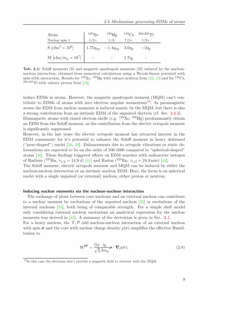
Tab. 2.1: Schiff moments (S) and magnetic quadrupole moments (M) induced by the nucleon-nucleon interaction, obtained from numerical calculations using a Woods-Saxon potential withspin-orbit interaction. Results for 129Xe, 199Hg with valence neutron from [43, 44] and for 133Cs,203,205Tl with valence proton from [45].
induce EDMs in atoms. However, the magnetic quadrupole moment (MQM) can’t con-tribute to EDMs of atoms with zero electron angular momentum10. In paramagneticatoms the EDM from nuclear moments is induced mainly by the MQM, but there is alsoa strong contribution from an intrinsic EDM of the unpaired electron (cf. Sec. 2.4.3).Diamagnetic atoms with closed electron shells (e.g. 129Xe, 199Hg) predominantly obtainan EDM from the Schiff moment, as the contribution from the electric octupole momentis significantly suppressed.However, in the last years the electric octupole moment has attracted interest in theEDM community for it’s potential to enhance the Schiff moment in heavy deformed(“pear-shaped”) nuclei [38, 39]. Enhancements due to octupole vibrations or static de-formations are expected to be on the order of 100-1000 compared to “spherical-shaped”atoms [40]. These findings triggered efforts on EDM searches with radioactive isotopesof Radium (225Ra, τ1/2 = 14.9 d) [41] and Radon (223Rn, τ1/2 = 24.3min) [42].The Schiff moment, electric octupole moment and MQM can be induced by either thenucleon-nucleon interaction or an intrinsic nucleon EDM. Here, the focus is on sphericalnuclei with a single unpaired (or external) nucleon, either proton or neutron.
Inducing nuclear moments via the nucleon-nucleon interactionThe exchange of pions between core nucleons and an external nucleon can contribute
to a nuclear moment by excitations of the unpaired nucleon [45] or excitations of theinternal nucleons [44], both being of comparable strength. For a simple shell modelonly considering external nucleon excitations an analytical expression for the nuclearmoments was derived in [45]. A summary of the derivation is given in Sec. A.1.For a heavy nucleus, the T ,P odd nucleon-nucleon interaction of an external nucleonwith spin σ and the core with nuclear charge density ρ(r) simplifies the effective Hamil-tonian to
HTP =GF√2
ηa2mp
σ ·∇ρ(r), (2.8)
10In this case the electrons don’t provide a magnetic field to interact with the MQM.
9
2 Electric dipole moment (EDM): Motivation, theory and experiments
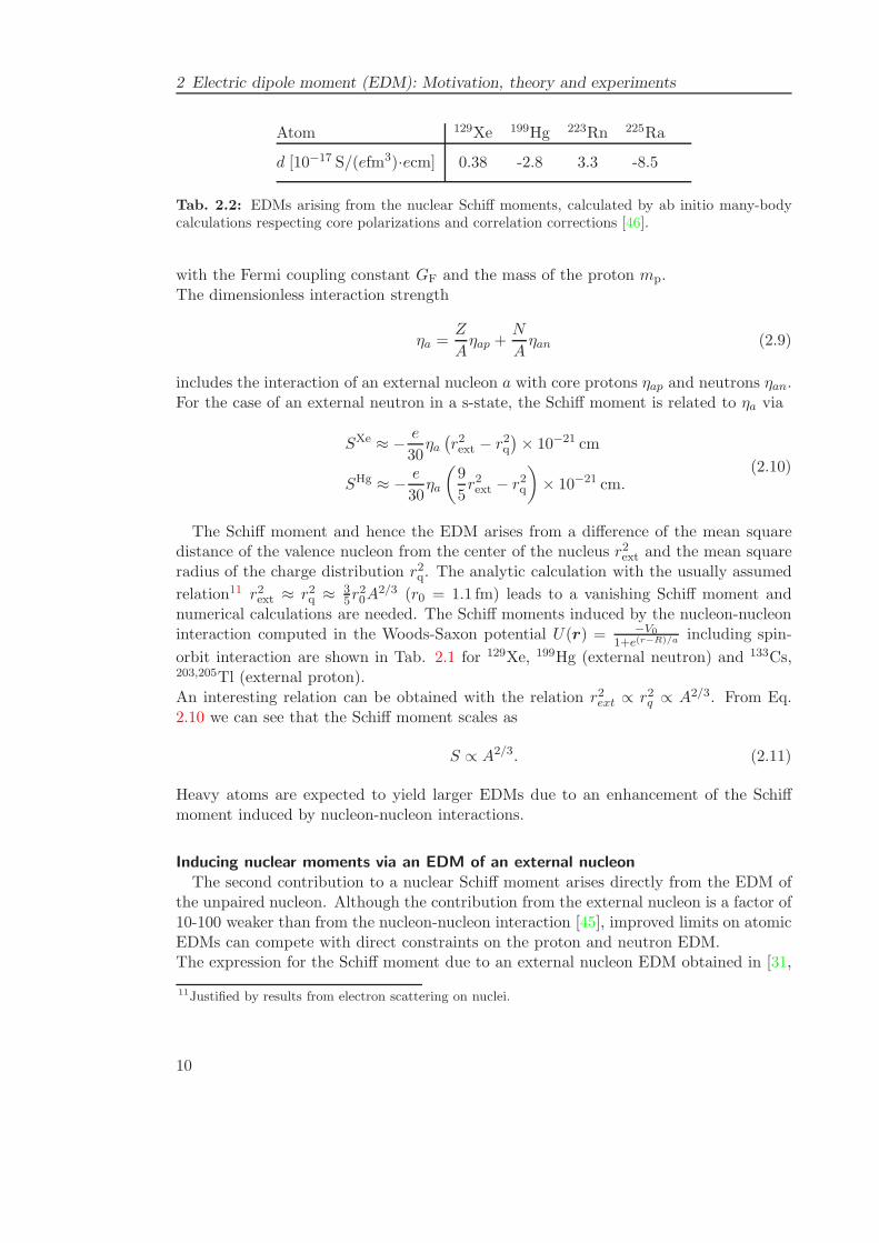
Atom 129Xe 199Hg 223Rn 225Ra
d [10−17 S/(efm3)·ecm] 0.38 -2.8 3.3 -8.5
Tab. 2.2: EDMs arising from the nuclear Schiff moments, calculated by ab initio many-bodycalculations respecting core polarizations and correlation corrections [46].
with the Fermi coupling constant GF and the mass of the proton mp.The dimensionless interaction strength
ηa =Z
Aηap +
N
Aηan (2.9)
includes the interaction of an external nucleon a with core protons ηap and neutrons ηan.For the case of an external neutron in a s-state, the Schiff moment is related to ηa via
SXe ≈ − e
30ηa(r2ext − r2q
)× 10−21 cm
SHg ≈ − e
30ηa
(9
5r2ext − r2q
)× 10−21 cm.
(2.10)
The Schiff moment and hence the EDM arises from a difference of the mean squaredistance of the valence nucleon from the center of the nucleus r2ext and the mean squareradius of the charge distribution r2q. The analytic calculation with the usually assumed
relation11 r2ext ≈ r2q ≈ 35r
20A
2/3 (r0 = 1.1 fm) leads to a vanishing Schiff moment andnumerical calculations are needed. The Schiff moments induced by the nucleon-nucleoninteraction computed in the Woods-Saxon potential U(r) = −V0
1+e(r−R)/a including spin-
orbit interaction are shown in Tab. 2.1 for 129Xe, 199Hg (external neutron) and 133Cs,203,205Tl (external proton).An interesting relation can be obtained with the relation r2ext ∝ r2q ∝ A2/3. From Eq.2.10 we can see that the Schiff moment scales as
S ∝ A2/3. (2.11)
Heavy atoms are expected to yield larger EDMs due to an enhancement of the Schiffmoment induced by nucleon-nucleon interactions.
Inducing nuclear moments via an EDM of an external nucleonThe second contribution to a nuclear Schiff moment arises directly from the EDM of
the unpaired nucleon. Although the contribution from the external nucleon is a factor of10-100 weaker than from the nucleon-nucleon interaction [45], improved limits on atomicEDMs can compete with direct constraints on the proton and neutron EDM.The expression for the Schiff moment due to an external nucleon EDM obtained in [31,
11Justified by results from electron scattering on nuclei.
10
2.4 Mechanisms generating EDMs of atoms
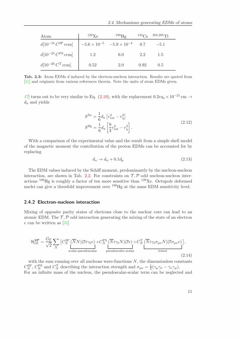
Atom 129Xe 199Hg 133Cs 203,205Tl
d[10−18 CSP ecm] −5.6× 10⁻⁵ −5.9× 10⁻⁴ 0.7 −5.1
d[10−23 CPS ecm] 1.2 6.0 2.2 1.5
d[10−20 CT ecm] 0.52 2.0 0.92 0.5
Tab. 2.3: Atom EDMs d induced by the electron-nucleon interaction. Results are quoted from[31] and originate from various references therein. Note the units of atom EDMs given.
47] turns out to be very similar to Eq. (2.10), with the replacement 0.2eηa×10−21 cm →dn and yields
SXe =1
6dn[r2ext − r2q
]
SHg =1
6dn
[9
3r2ext − r2q
].
(2.12)
With a comparison of the experimental value and the result from a simple shell modelof the magnetic moment the contribution of the proton EDMs can be accounted for byreplacing
dn → dn + 0.1dp (2.13)
The EDM values induced by the Schiff moment, predominantly by the nucleon-nucleoninteraction, are shown in Tab. 2.2. For constraints on T ,P odd nucleon-nucleon inter-actions 199Hg is roughly a factor of ten more sensitive than 129Xe. Octupole deformednuclei can give a threefold improvement over 199Hg at the same EDM sensitivity level.
2.4.2 Electron-nucleon interaction
Mixing of opposite parity states of electrons close to the nuclear core can lead to anatomic EDM. The T ,P odd interaction generating the mixing of the state of an electrone can be written as [31]
HTPeN =
GF√2
∑
N
[CSPN (NN)(eiγ5e)
scalar-pseudoscalar
+CPSN (Niγ5N)(ee)
pseudoscaler-scalar
+CTN (Niγ5σµνN)(eσµνe)
tensor
],
(2.14)
with the sum running over all nucleons wave-functions N , the dimensionless constantsCSPN , CPS
N and CTN describing the interaction strength and σµν = 1
2(γµγν − γνγµ).For an infinite mass of the nucleus, the pseudoscalar-scalar term can be neglected and
11
2 Electric dipole moment (EDM): Motivation, theory and experiments
Atom 129Xe 199Hg 133Cs 203,205Tl
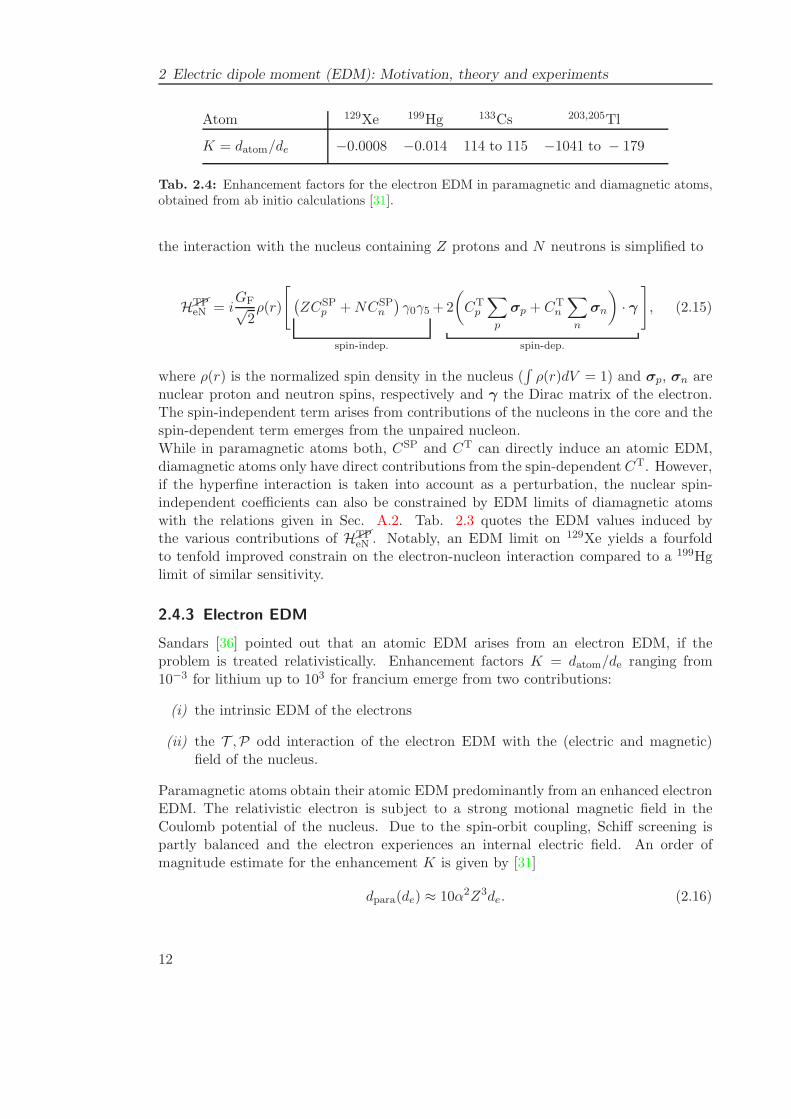
K = datom/de −0.0008 −0.014 114 to 115 −1041 to − 179
Tab. 2.4: Enhancement factors for the electron EDM in paramagnetic and diamagnetic atoms,obtained from ab initio calculations [31].
the interaction with the nucleus containing Z protons and N neutrons is simplified to
HTPeN = i
GF√2ρ(r)
[(ZCSP
p +NCSPn
)γ0γ5
spin-indep.
+2
(CTp
∑
p
σp + CTn
∑
n
σn
)· γ
spin-dep.
], (2.15)
where ρ(r) is the normalized spin density in the nucleus (∫ρ(r)dV = 1) and σp, σn are
nuclear proton and neutron spins, respectively and γ the Dirac matrix of the electron.The spin-independent term arises from contributions of the nucleons in the core and thespin-dependent term emerges from the unpaired nucleon.While in paramagnetic atoms both, CSP and CT can directly induce an atomic EDM,diamagnetic atoms only have direct contributions from the spin-dependent CT. However,if the hyperfine interaction is taken into account as a perturbation, the nuclear spin-independent coefficients can also be constrained by EDM limits of diamagnetic atomswith the relations given in Sec. A.2. Tab. 2.3 quotes the EDM values induced bythe various contributions of HTP
eN . Notably, an EDM limit on 129Xe yields a fourfoldto tenfold improved constrain on the electron-nucleon interaction compared to a 199Hglimit of similar sensitivity.
2.4.3 Electron EDM
Sandars [36] pointed out that an atomic EDM arises from an electron EDM, if theproblem is treated relativistically. Enhancement factors K = datom/de ranging from10−3 for lithium up to 103 for francium emerge from two contributions:
(i) the intrinsic EDM of the electrons
(ii) the T ,P odd interaction of the electron EDM with the (electric and magnetic)field of the nucleus.
Paramagnetic atoms obtain their atomic EDM predominantly from an enhanced electronEDM. The relativistic electron is subject to a strong motional magnetic field in theCoulomb potential of the nucleus. Due to the spin-orbit coupling, Schiff screening ispartly balanced and the electron experiences an internal electric field. An order ofmagnitude estimate for the enhancement K is given by [31]
dpara(de) ≈ 10α2Z3de. (2.16)
12
2.5 Sensitivity of EDMs to physics beyond the SM
1e-35
1e-34
1e-33
1e-32
1e-31
1e-30
1e-29
1e-28
1e-27
1e-26
1e-25
198
0
199
0
200
0
201
0
202
0
Theory predictions
n Hg Xe
SM
SM
exte
ntions
SM
SM
exte
ntions
SM
SM
exte
ntions
ED
M lim
it [ecm
]
Year
neutron199
Hg129
Xe
e- (YbF, ThO)
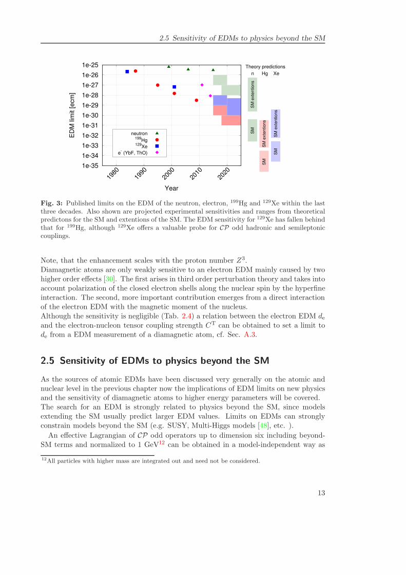
Fig. 3: Published limits on the EDM of the neutron, electron, 199Hg and 129Xe within the lastthree decades. Also shown are projected experimental sensitivities and ranges from theoreticalpredictons for the SM and extentions of the SM. The EDM sensitivity for 129Xe has fallen behindthat for 199Hg, although 129Xe offers a valuable probe for CP odd hadronic and semileptoniccouplings.
Note, that the enhancement scales with the proton number Z3.Diamagnetic atoms are only weakly sensitive to an electron EDM mainly caused by twohigher order effects [30]. The first arises in third order perturbation theory and takes intoaccount polarization of the closed electron shells along the nuclear spin by the hyperfineinteraction. The second, more important contribution emerges from a direct interactionof the electron EDM with the magnetic moment of the nucleus.Although the sensitivity is negligible (Tab. 2.4) a relation between the electron EDM deand the electron-nucleon tensor coupling strength CT can be obtained to set a limit tode from a EDM measurement of a diamagnetic atom, cf. Sec. A.3.
2.5 Sensitivity of EDMs to physics beyond the SM
As the sources of atomic EDMs have been discussed very generally on the atomic andnuclear level in the previous chapter now the implications of EDM limits on new physicsand the sensitivity of diamagnetic atoms to higher energy parameters will be covered.The search for an EDM is strongly related to physics beyond the SM, since modelsextending the SM usually predict larger EDM values. Limits on EDMs can stronglyconstrain models beyond the SM (e.g. SUSY, Multi-Higgs models [48], etc. ).
An effective Lagrangian of CP odd operators up to dimension six including beyond-SM terms and normalized to 1 GeV12 can be obtained in a model-independent way as
12All particles with higher mass are integrated out and need not be considered.
13
2 Electric dipole moment (EDM): Motivation, theory and experiments
π
Σ
+
nn
γ
c,t c,t
g
s d
u,du,d
Wγ
f f
γ∼
ff∼
∼
L
R
L
R
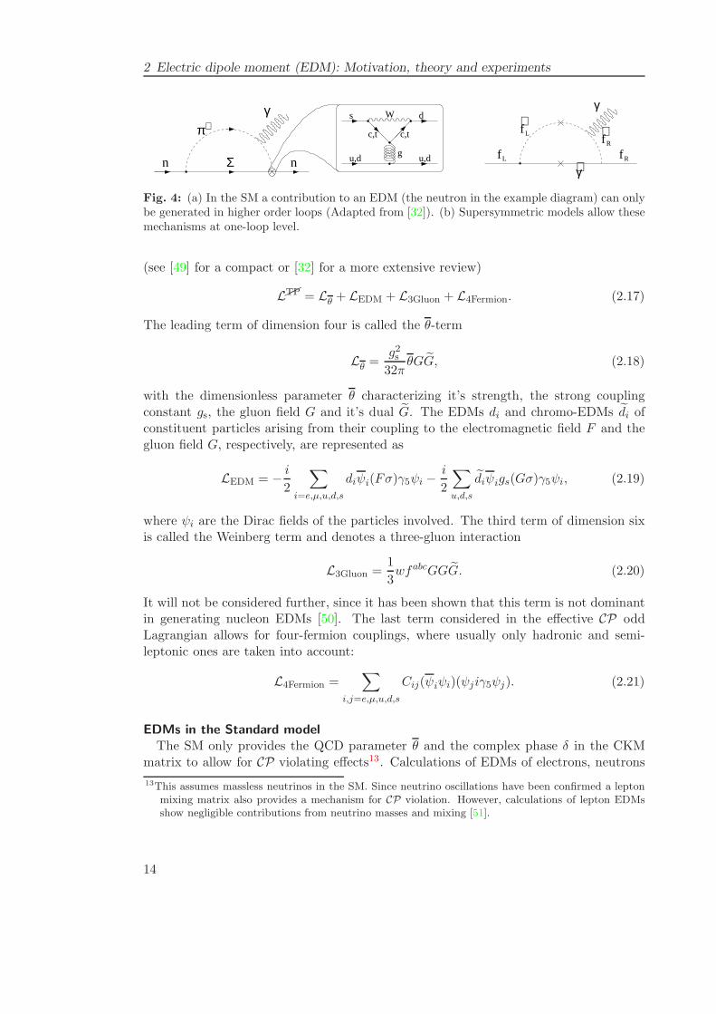
Fig. 4: (a) In the SM a contribution to an EDM (the neutron in the example diagram) can onlybe generated in higher order loops (Adapted from [32]). (b) Supersymmetric models allow thesemechanisms at one-loop level.
(see [49] for a compact or [32] for a more extensive review)
LTP = Lθ + LEDM + L3Gluon + L4Fermion. (2.17)
The leading term of dimension four is called the θ-term
Lθ =g2s32π
θGG, (2.18)
with the dimensionless parameter θ characterizing it’s strength, the strong couplingconstant gs, the gluon field G and it’s dual G. The EDMs di and chromo-EDMs di ofconstituent particles arising from their coupling to the electromagnetic field F and thegluon field G, respectively, are represented as
LEDM = − i
2
∑
i=e,µ,u,d,s
diψi(Fσ)γ5ψi −i
2
∑
u,d,s
diψigs(Gσ)γ5ψi, (2.19)
where ψi are the Dirac fields of the particles involved. The third term of dimension sixis called the Weinberg term and denotes a three-gluon interaction
L3Gluon =1
3wfabcGGG. (2.20)
It will not be considered further, since it has been shown that this term is not dominantin generating nucleon EDMs [50]. The last term considered in the effective CP oddLagrangian allows for four-fermion couplings, where usually only hadronic and semi-leptonic ones are taken into account:
L4Fermion =∑
i,j=e,µ,u,d,s
Cij(ψiψi)(ψjiγ5ψj). (2.21)
EDMs in the Standard modelThe SM only provides the QCD parameter θ and the complex phase δ in the CKM
matrix to allow for CP violating effects13. Calculations of EDMs of electrons, neutrons
13This assumes massless neutrinos in the SM. Since neutrino oscillations have been confirmed a leptonmixing matrix also provides a mechanism for CP violation. However, calculations of lepton EDMsshow negligible contributions from neutrino masses and mixing [51].
14
2.5 Sensitivity of EDMs to physics beyond the SM
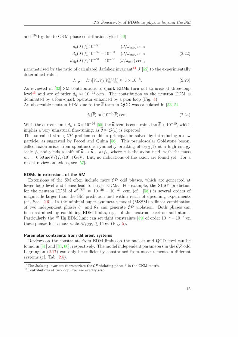
and 199Hg due to CKM phase contributions yield [49]
de(J) . 10−38 (J/Jexp) ecm
dn(J) . 10−32 − 10−31 (J/Jexp) ecm
dHg(J) . 10−34 − 10−35 (J/Jexp) ecm,
(2.22)
parametrized by the ratio of calculated Jarlskog invariant14 J [52] to the experimentallydetermined value
Jexp = Im[VusVcbV∗
csV∗
ub] ≈ 3× 10⁻⁵. (2.23)
As reviewed in [32] SM contributions to quark EDMs turn out to arise at three-looplevel15 and are of order dq ≈ 10−34 ecm. The contribution to the neutron EDM isdominated by a four-quark operator enhanced by a pion loop (Fig. 4).An observable neutron EDM due to the θ term in QCD was calculated in [53, 54]
dn(θ) ≈ (10−16θ) ecm. (2.24)
With the current limit dn < 3× 10⁻²⁶ [55] the θ term is constrained to θ < 10−10, whichimplies a very unnatural fine-tuning, as θ ≈ O(1) is expected.This so called strong CP problem could in principal be solved by introducing a newparticle, as suggested by Peccei and Quinn [56]. This pseudoscalar Goldstone boson,called axion arises from spontaneous symmetry breaking of UPQ(1) at a high energyscale fa and yields a shift of θ → θ + a/fa, where a is the axion field, with the massma = 0.60meV/(fa/10
10)GeV. But, no indications of the axion are found yet. For arecent review on axions, see [57].
EDMs in extensions of the SMExtensions of the SM often include more CP odd phases, which are generated at
lower loop level and hence lead to larger EDMs. For example, the SUSY predictionfor the neutron EDM of dSUSY
n ≈ 10−26 − 10−30 ecm (cf. [58]) is several orders ofmagnitude larger than the SM prediction and within reach of upcoming experiments(cf. Sec. 2.6). In the minimal super-symmetric model (MSSM) a linear combinationof two independent phases θµ and θA can generate CP violation. Both phases canbe constrained by combining EDM limits, e.g. of the neutron, electron and atoms.Particularly the 199Hg EDM limit can set tight constraints [59] of order 10−2 − 10−3 onthese phases for a mass scale MSUSY . 1Tev (Fig. 5).
Parameter contraints from different systemsReviews on the constraints from EDM limits on the nuclear and QCD level can be
found in [31] and [33, 60], respectively. The model independent parameters in the CP oddLagrangian (2.17) can only be sufficiently constrained from measurements in differentsystems (cf. Tab. 2.5).
14The Jarlskog invariant characterizes the CP violating phase δ in the CKM matrix.15Contributions at two-loop level are exactly zero.
15
2 Electric dipole moment (EDM): Motivation, theory and experiments
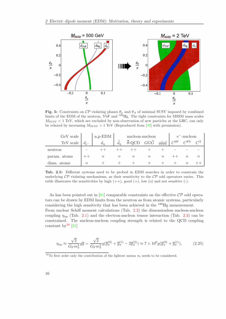
Fig. 5: Constraints on CP violating phases θµ and θA of minimal SUSY imposed by combinedlimits of the EDM of the neutron, YbF and 199Hg. The tight constraints for MSSM mass scalesMSUSY < 1 TeV, which are excluded by non-observation of new particles at the LHC, can onlybe relaxed by increasing MSUSY > 1 TeV (Reproduced from [49] with permission).
GeV scale n,p-EDM nucleon-nucleon e−-nucleon
TeV scale de− dq dq θ-QCD GGG qqqq CSP CPS CT
neutron - ++ ++ ++ + + - - -
param. atoms ++ o o o o o ++ o o
diam. atoms o + + + + + + o ++
Tab. 2.5: Different systems need to be probed in EDM searches in order to constrain theunderlying CP violating mechanisms, as their sensitivity to the CP odd operators varies. Thistable illustrates the sensitivities by high (++), good (+), low (o) and not sensitive (-).
As has been pointed out in [61] comparable constraints on the effective CP odd opera-tors can be drawn by EDM limits from the neutron as from atomic systems, particularlyconsidering the high sensitivity that has been achieved in the 199Hg measurement.From nuclear Schiff moment calculations (Tab. 2.2) the dimensionless nucleon-nucleoncoupling ηnp (Tab. 2.1) and the electron-nucleon tensor interaction (Tab. 2.3) can beconstrained. The nucleon-nucleon coupling strength is related to the QCD couplingconstant by16 [31]
ηnp ≈√2
GFm2π
gg =
√2
GFm2π
g(g(0)π + g(1)π − 2g(2)π ) ≈ 7× 10⁶g(g(0)π + g(1)π ), (2.25)
16To first order only the contribution of the lightest meson π0 needs to be considered.
16
2.6 Experimental status and prospects of EDM searches
with the strong coupling constant g = 13.6, the pion mass mπ and the isoscalar g(0)π ,
isovector g(1)π and isotensor g
(2)π couplings. The latter turns out to be suppressed [33].
Note, that θ is related to g as [53]
|g| ≈ |g(0)π + g(1)π | ≈ 0.027 θ. (2.26)
Constraints on the chromo EDMs of up- and down-quark can be obtained from [62]
g = 2(du − dd)/10−14 ecm. (2.27)
For the description of four fermion interactions phenomenological parameters for quark-quark and semi-leptonic interactions are defined and respective limits extracted, cf. [31].The neutron EDM sets a limit on the parameter θ (cf. Eq. (2.24)) and the quark andchromo EDMs via [63]
dn = (1± 0.5)[0.55e(dd + 0.5du) + 0.7(dd − 0.25du)]. (2.28)
The EDM limit obtained from paramagnetic atoms dominantly imposes constraints onan electron EDM de and the scalar-pseudoscalar coupling CSP.Diamagnetic atoms are particularly sensitive to hadronic sources and the spin-dependentelectron-nucleon coupling (Eq. 2.15). In higher order also the electron EDM and CSP
contribute.To disentangle the many T ,P odd parameters de, C
SP, CT, g(0)π , g
(1)π and the neutron and
proton EDM dn, dp various EDM limits on different systems are needed. A summaryon improvements on the parameters from additional new EDM limits of 129Xe, 225Ra,the neutron and their combination is given in [60]. Adding an 129Xe EDM limit of ≈10−29 ecm to the current 199Hg limit the constraints on CT, g
(0)π , g
(1)π would be improved
by factors of roughly 10, 3 and 2, respectively. The effective field theory [60] and nuclearcalculations [31] identify the importance of new EDM limits of additional diamagneticsystems, even though the 199Hg measurement already provides an excellent sensitivity.
2.6 Experimental status and prospects of EDM searches
In this section the basic experimental method used in state-of-the-art EDM searches willbe introduced. A detailed discussion focused on the most recent measurement on 129Xeis postponed to Sec. 4, where also new approaches to further improve the sensitivity arepresented.Various efforts of EDM searches have been undertaken after the possibility of non-zeroEDMs was suggested about 60 years ago [64]. In the first EDM experiment Ramseyused the technique of separated oscillatory fields, which he developed and adapted to aneutron beam to search for an EDM [65] (for a recent review of the method, see [66]).Most EDM experiments nowadays, no matter whether the system used is the neutron,para- or diamagnetic atoms are looking for a deviation of the Larmor precession fre-quency ωL when applying an additional electric field E parallel to a magnetic field B.The Zeeman splitting in a two-level system reads
~ωL = 2(µ.B − d.E) (2.29)
17
2 Electric dipole moment (EDM): Motivation, theory and experiments
Experiment [ecm] SM pred. References
Current Proposed [ecm] exp. theor.
n 3× 10⁻²⁶ ∼ 10−28 ∼ 10−31 − 10−32 [55] [68]
e− 8.7× 10⁻²⁹ ∼ 10−32 . 10−38 [69] [32, 70]
129Xe 0.7±3.3×10⁻²⁷ ∼ 10−29 ∼ 10−33 − 10−34 [71] [45]
199Hg 3.1× 10⁻²⁹ . 10−29 ∼ 10−34 − 10−35 [67] [49]
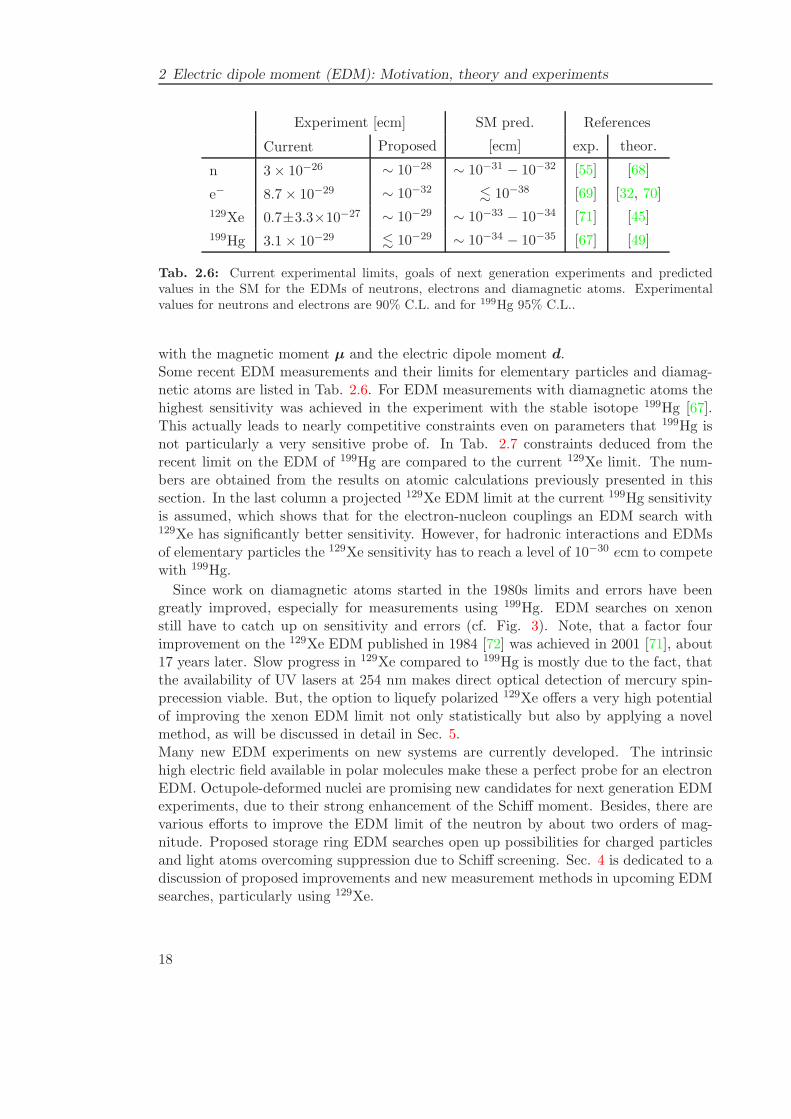
Tab. 2.6: Current experimental limits, goals of next generation experiments and predictedvalues in the SM for the EDMs of neutrons, electrons and diamagnetic atoms. Experimentalvalues for neutrons and electrons are 90% C.L. and for 199Hg 95% C.L..
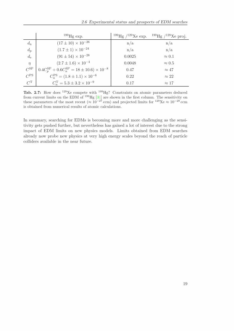
with the magnetic moment µ and the electric dipole moment d.Some recent EDM measurements and their limits for elementary particles and diamag-netic atoms are listed in Tab. 2.6. For EDM measurements with diamagnetic atoms thehighest sensitivity was achieved in the experiment with the stable isotope 199Hg [67].This actually leads to nearly competitive constraints even on parameters that 199Hg isnot particularly a very sensitive probe of. In Tab. 2.7 constraints deduced from therecent limit on the EDM of 199Hg are compared to the current 129Xe limit. The num-bers are obtained from the results on atomic calculations previously presented in thissection. In the last column a projected 129Xe EDM limit at the current 199Hg sensitivityis assumed, which shows that for the electron-nucleon couplings an EDM search with129Xe has significantly better sensitivity. However, for hadronic interactions and EDMsof elementary particles the 129Xe sensitivity has to reach a level of 10−30 ecm to competewith 199Hg.
Since work on diamagnetic atoms started in the 1980s limits and errors have beengreatly improved, especially for measurements using 199Hg. EDM searches on xenonstill have to catch up on sensitivity and errors (cf. Fig. 3). Note, that a factor fourimprovement on the 129Xe EDM published in 1984 [72] was achieved in 2001 [71], about17 years later. Slow progress in 129Xe compared to 199Hg is mostly due to the fact, thatthe availability of UV lasers at 254 nm makes direct optical detection of mercury spin-precession viable. But, the option to liquefy polarized 129Xe offers a very high potentialof improving the xenon EDM limit not only statistically but also by applying a novelmethod, as will be discussed in detail in Sec. 5.Many new EDM experiments on new systems are currently developed. The intrinsichigh electric field available in polar molecules make these a perfect probe for an electronEDM. Octupole-deformed nuclei are promising new candidates for next generation EDMexperiments, due to their strong enhancement of the Schiff moment. Besides, there arevarious efforts to improve the EDM limit of the neutron by about two orders of mag-nitude. Proposed storage ring EDM searches open up possibilities for charged particlesand light atoms overcoming suppression due to Schiff screening. Sec. 4 is dedicated to adiscussion of proposed improvements and new measurement methods in upcoming EDMsearches, particularly using 129Xe.
18
2.6 Experimental status and prospects of EDM searches
199Hg exp. 199Hg /129Xe exp. 199Hg /129Xe proj.
dn (17± 10) × 10−26 n/a n/a
dp (1.7 ± 1)× 10−24 n/a n/a
de (91± 54) × 10−28 0.0025 ≈ 0.1
η (2.7 ± 1.6) × 10−4 0.0048 ≈ 0.5
CSP 0.4CSPp + 0.6CSP
n = 18± 10.6) × 10−8 0.47 ≈ 47
CPS CPSn = (1.8 ± 1.1) × 10−6 0.22 ≈ 22
CT CTn = 5.3 ± 3.2× 10⁻⁹ 0.17 ≈ 17
Tab. 2.7: How does 129Xe compete with 199Hg? Constraints on atomic parameters deducedfrom current limits on the EDM of 199Hg [31] are shown in the first column. The sensitivity onthese parameters of the most recent (≈ 10−27 ecm) and projected limits for 129Xe ≈ 10−29 ecmis obtained from numerical results of atomic calculations.
In summary, searching for EDMs is becoming more and more challenging as the sensi-tivity gets pushed further, but nevertheless has gained a lot of interest due to the strongimpact of EDM limits on new physics models. Limits obtained from EDM searchesalready now probe new physics at very high energy scales beyond the reach of particlecolliders available in the near future.
19

3 Optimizing the parameter space for anew 129Xe EDM search
A key to new EDM experiments, particularly using novel concepts, is evaluation of theparameter space. For that purpose the theoretical and experimental principles of atomicphysics, spin precession and superconducting magnetometers are introduced in this sec-tion. The first part will be dedicated to some basic atomic physics, before advancing tooptical pumping of alkali atoms and spin-exchange to the noble gas nuclei. A discus-sion of spin relaxation of 129Xe and 3He will be given in Sec. 3.3 with emphasis on therelaxation mechanisms in gas, liquid and solid phases of 129Xe. A short introductionto superconductivity and the benefits of superconducting quantum interference devices(SQUIDs) for detection of spin-precession will conclude this section.
3.1 Atomic physics
For the course of this section on optical pumping and spin precession physics somefundamentals of atomic magnetic moments, level splitting and response to externallyapplied magnetic fields are needed. Most of this is treated in standard textbooks, e.g.[73].
3.1.1 Atomic magnetic moments and level splitting
The terminology characterizing electronic energy levels follows n2S+1LJ, with the princi-pal quantum number n, the multiplicity 2S+1, the orbital angular momentum L and thetotal angular momentum J . L represents the orbital angular momentum l = 0, 1, 2, ...,but for historic reasons l = S,P,D,F, ... is commonly used.The electronic magnetic moment µJ of an atom has contributions from the electron’sorbital angular momentum L and it’s spin S. The spin-orbit coupling leads to the totalangular momentum J = L+S yielding the magnetic moment due to the electron cloud
µJ = −gJµB~J , where gJ = 1 +
J2 + S2 −L2
2J2(3.1)
is the Lande factor and the Bohr magneton µB = e~2me
. The total angular momentumtakes on values of L− S ≤ J ≤ L+ S in integer steps.The nuclear magnetic moment µI is determined by the sum of the combination of spinsand orbital angular momenta of all nucleons I =
∑i(si + li) as
µI = gIµN~
I, (3.2)
21
3 Optimizing the parameter space for a new 129Xe EDM search
5S
−1/2
−1/2
mixingcollisional
σ+
Γ
1/2
3/25P
5P
1/2
Jm
5S
5P
spin−orbit Zeeman splittingcoupling
794.
78nm
780.
24nm
D2D1
1/2
1/2
−3/2
−1/2
3/2
1/2
50%50%
Rb
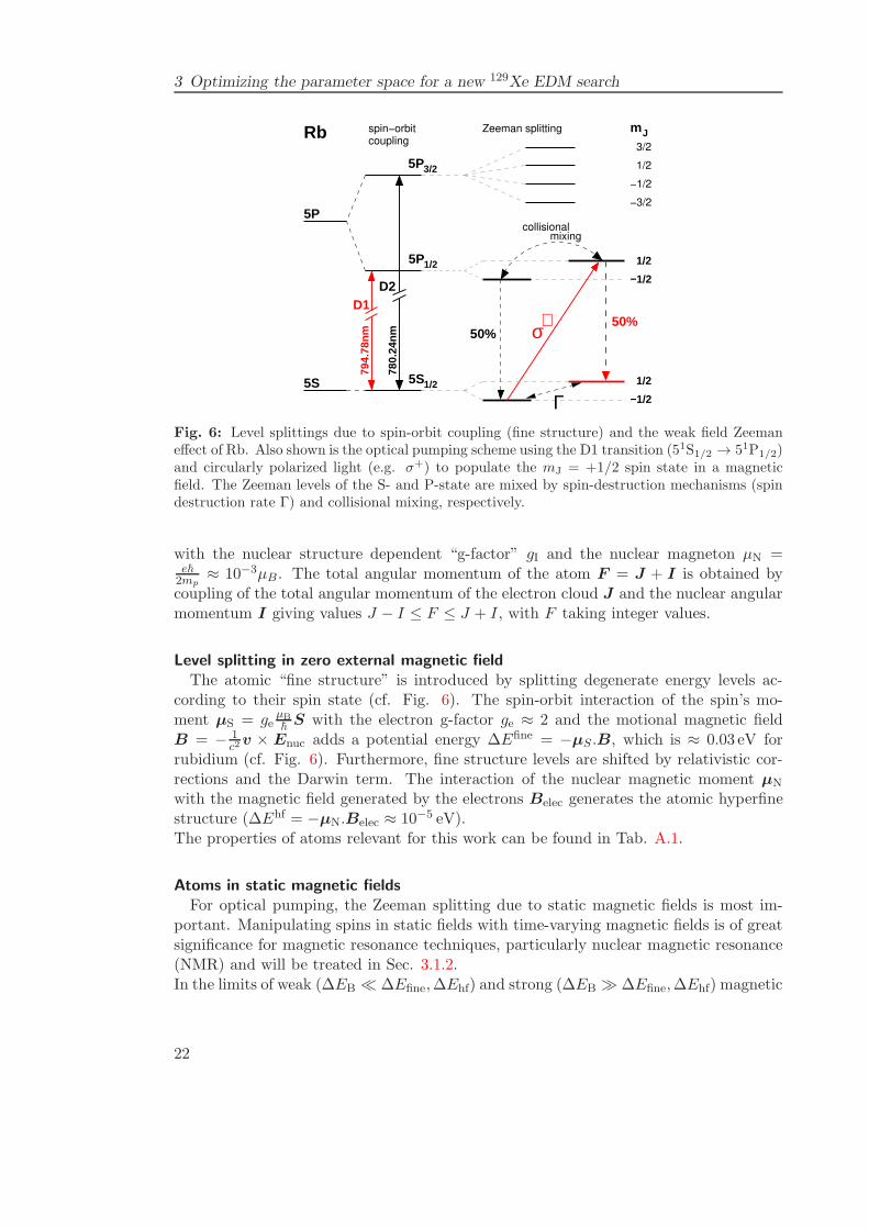
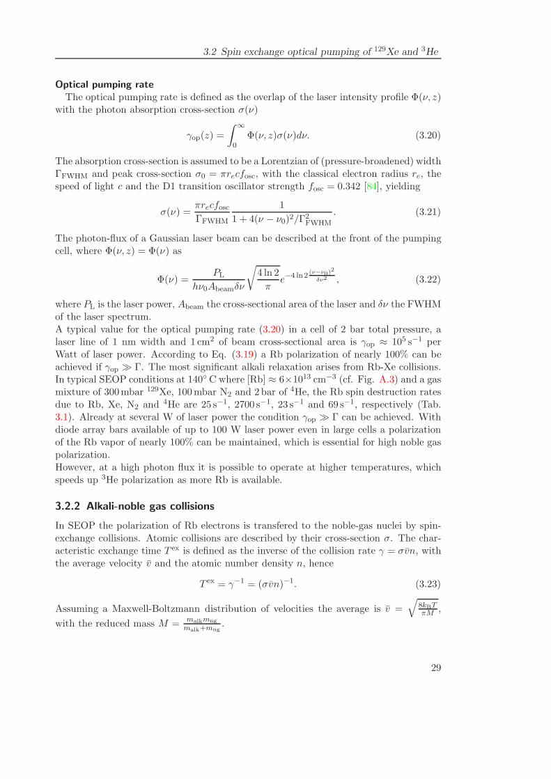
Fig. 6: Level splittings due to spin-orbit coupling (fine structure) and the weak field Zeemaneffect of Rb. Also shown is the optical pumping scheme using the D1 transition (51S1/2 → 51P1/2)and circularly polarized light (e.g. σ+) to populate the mJ = +1/2 spin state in a magneticfield. The Zeeman levels of the S- and P-state are mixed by spin-destruction mechanisms (spindestruction rate Γ) and collisional mixing, respectively.
with the nuclear structure dependent “g-factor” gI and the nuclear magneton µN =e~2mp
≈ 10−3µB . The total angular momentum of the atom F = J + I is obtained bycoupling of the total angular momentum of the electron cloud J and the nuclear angularmomentum I giving values J − I ≤ F ≤ J + I, with F taking integer values.
Level splitting in zero external magnetic fieldThe atomic “fine structure” is introduced by splitting degenerate energy levels ac-
cording to their spin state (cf. Fig. 6). The spin-orbit interaction of the spin’s mo-ment µS = ge
µB~S with the electron g-factor ge ≈ 2 and the motional magnetic field
B = − 1c2v × Enuc adds a potential energy ∆Efine = −µS .B, which is ≈ 0.03 eV for
rubidium (cf. Fig. 6). Furthermore, fine structure levels are shifted by relativistic cor-rections and the Darwin term. The interaction of the nuclear magnetic moment µN
with the magnetic field generated by the electrons Belec generates the atomic hyperfinestructure (∆Ehf = −µN.Belec ≈ 10−5 eV).The properties of atoms relevant for this work can be found in Tab. A.1.
Atoms in static magnetic fieldsFor optical pumping, the Zeeman splitting due to static magnetic fields is most im-
portant. Manipulating spins in static fields with time-varying magnetic fields is of greatsignificance for magnetic resonance techniques, particularly nuclear magnetic resonance(NMR) and will be treated in Sec. 3.1.2.In the limits of weak (∆EB ≪ ∆Efine,∆Ehf) and strong (∆EB ≫ ∆Efine,∆Ehf) magnetic
22
3.1 Atomic physics
fields the breaking of degeneracy is the Zeeman and Paschen-Back effect, respectively.An external magnetic field splits up the fine and hyperfine levels into 2J +1 and 2F +1energy levels, respectively. Depending on the applied magnetic field the electron angularmomenta S (spin) and L (orbit) are either coupled to J = S+L (weak field) or uncou-pled (strong field). The level splittings due to angular momenta couplings are of order10−2 eV (spin-orbit) and 10−5 eV (electron-nuclear angular momenta), hence magneticfields B ≪ 0.1T are considered weak.For a magnetic field B in z direction (the quantization axis) the separation of the fineand hyperfine structure levels are
∆EfineB = gJmJµBBz and ∆Ehf
B = gFmFµBBz. (3.3)
The magnetic quantum numbersmJ and mF take on integer values from −J~, ..., J~ and−F~, ..., F~, respectively. In (3.3) gJ is the Lande factor (Eq. (3.1)) and
gF = gJF (F + 1) + J(J + 1)− I(I + 1)
2F (F + 1)+ gI
F (F + 1) + I(I + 1)− J(J + 1)
2F (F + 1), (3.4)
where the second term is often negligible as gI ≈ 10−3gJ.
In optical pumping techniques the Zeeman level splitting is utilized to populate oneelectronic spin state of an alkali metal, e.g. rubidium (cf. Fig. 6 and Sec. 3.2) inmagnetic fields of 1 − 10mT. Under these conditions the hyperfine structure is notresolved.
3.1.2 Nuclear magnetic resonance
Here, I will only consider nuclear magnetic resonance of atoms with nuclear spin I = 12
applying to 1H, 3He and 129Xe. Then, the nuclear Zeeman levels (m−1/2,m+1/2) areseparated in a magnetic field B by
∆E = 2µIB = hγIB = ~ωL, (3.5)
with the nuclear magnetic moment µI, the gyromagnetic ratio γI = γ and the definitionof the Larmor frequency
ωL = 2πγB. (3.6)
In nuclear magnetic resonance (NMR) the fundamental processes are absorption andstimulated emission arising from the transition between Zeeman energy levels. Selectionrules imply ∆mI = ±1. This quantum-mechanical two-level system with Iz = ±1
2~
and I2 = I(I + 1)~2 = 34~
2 can be macroscopically described by the difference of levelpopulation ∆N = N+ −N−. The polarization P of a sample is then defined as
P =N+ −N−
N+ +N−. (3.7)
23
3 Optimizing the parameter space for a new 129Xe EDM search
In thermal equilibrium the levels are populated according to the Boltzmann distributione∆E/kBT , yielding
Ptherm =1− e
2µBkBT
1 + e2µBkBT
≈ µB
kBT. (3.8)
The magnetization M is defined as the magnetic moment density and for a spin-polarizedtwo-level system one obtains
M =1
V
∑
N
µ =∆N
Vµ =
NP
Vµ, (3.9)
with the sample volume V , the total number of magnetic moments N , the degree ofpolarization P and the magnetic moment of the constituents µ. A polarization vectorcan be defined as P = PM/M .The dynamics of a macroscopic magnetization in a magnetic field can be understood inthe following way. A magnetic moment initially not aligned with a static magnetic fieldaxis feels a torque according to µ × B and starts precessing around the holding field.The torque represents a change in total nuclear angular momentum I = µ/γ, hence
dI
dt=
1
γ
dµ
dt= µ×B. (3.10)
Since the macroscopic magnetization is proportional to the expectation value 〈µ〉, weget an equation describing the precession of the magnetization M as
dM
dt= γM ×B. (3.11)
Assume for simplicity, that the static magnetic field is applied in z direction B =(0, 0, Bz). Because the spin system can exchange energy with the surrounding (e.g.solid lattice, walls, etc.) the magnetization Mz along B is relaxing to it’s thermal equi-librium value, cf. Eq. (3.8), in a characteristic time T1, called spin-lattice, longitudinalor simply “T1” relaxation time. Additionally, magnetization in the x,y plane Mx,My
relaxes to thermal equilibrium within a characteristic time due to interactions of neigh-bouring spins. These locally generate magnetic fields making the spin precession frequen-cies diverge. The characteristic time of this spin-spin or transverse relaxation is called“T2””relaxation time. In real world experiments the term “T ∗
2 ” is often used including re-laxation effects due to gradients of applied or residual magnetic fields: 1
T ∗
2= 1
T2+ 1
T grad2
.
Both longitudinal and transverse relaxation mechanisms were phenomenologically in-cluded in Bloch’s equations [74] yielding the time evolution of a magnetization vector ina magnetic field Bz,
dMx
dt= γMyBz −
Mx
T2dMy
dt= −γMxBz −
My
T2dMz
dt= −Mz −M0
T1,
(3.12)
24
3.2 Spin exchange optical pumping of 129Xe and 3He
where M0 denotes the equilibrium magnetization. The equations of Bloch were general-ized by the inclusion of a diffusion term yielding the Bloch-Torrey equations [75].
3.1.3 Time-varying magnetic fields
To measure spin precession one needs to manipulate the polarization vector initiallyaligned along a magnetic field Bz. To detect the precession the polarization vectorneeds to be tipped by an angle θ, so that the precessing magnetization of the sampleinduces a voltage in a pickup loop.One way to achieve the misalignment is using an oscillating RF field pulse of amplitude2B1, frequency ω⊥ and duration τ , which is applied perpendicular to the Bz-axis. In therotating frame it can be shown, that if ω⊥ equals the Larmor frequency the magneticfield in z-direction is zero and the magnetization is precessing away from Bz at the Rabifrequency γB1 [76]. Hence, with a pulse of duration τ the tipping angle is
θ = γB1τ. (3.13)
From the usually neglected counter-rotating component of B⊥ the Bloch-Siegert shift
of the Larmor precession frequency ofB2
1
4B20arises [77]. Choosing the amplitude of the
oscillating field B1 to be less than < B010 limits the shift to less than ≈ 1%. The rotation
of the magnetization under off-resonant conditions can be evaluated when introducingthe oscillating magnetic field B⊥ = Bx,y sin(ω⊥t) in the Bloch equations (Eq. 3.12).The polarization vector can also be misaligned from Bz by a non-adiabatic magnetic fieldchange. The adiabatic condition assures that spins can follow a magnetic field change,e.g. the Larmor precession frequency ωL must be much larger than rotation frequencyof the total magnetic field ωrot
B , hence
ωL ≫ ωrotB . (3.14)
If the total field is changed fast enough to make the switching process non-adiabatic,the spins start precessing around the final magnetic field direction. In contrast to thisthe transport of polarized gas needs to be adiabatic to preserve polarization while spinsmove through different magnetic field regions.
3.2 Spin exchange optical pumping of 129Xe and 3He
The magnitude of the signal generated by a spin-polarized sample (e.g. by induction ina pickup loop) scales with the magnetization (3.9), hence with the number of polarizedatoms or nuclei. The thermal polarization of a sample (Eq. (3.8)) described by theBoltzmann distribution is very small even at lowest temperatures and strongest magneticfields. At room temperature the population difference is of order 10−9/mT. The degreeof polarization can be enhanced by several orders of magnitude by applying opticalpumping techniques.The nuclear spins of both 3He and 129Xe can be efficiently polarized by spin-exchange
25
3 Optimizing the parameter space for a new 129Xe EDM search
optical pumping (SEOP)17, which was first demonstrated for 3He and 129Xe by Bouchiat[79] and Grover [80], respectively. In SEOP electrons of an alkali vapor are polarized bycircularly polarized light (cf. Fig. 6) and the electron polarization is transfered to noblegas nuclei by exchange collisions. A general review of optical pumping and SEOP canbe found in [81] and [82], respectively. A more recent review particularly focusing onrecent developments in SEOP of 3He is given in [83].Note, that the nuclear spin of 199Hg can be more directly polarized by depopulationpumping of the ground state 1S0 to the excited state 3P1 using circularly polarized lightwith a wavelength of 254 nm. In a magnetic field the angular momentum of the photonis transfered to the nucleus due to the strong hyperfine coupling, hence populating theZeeman state m+1/2 (m−1/2) by σ
+ (σ−) photons, respectively. The availability of UVlasers of the required wavelength makes 199Hg very attractive, particularly because thespin precession can also be read out optically in a pump-probe scheme. This is one ofthe many reasons for the superior sensitivity of the 199Hg EDM measurement.
3.2.1 Optical pumping of alkali metals
The alkali metals rubidium and potassium are of relevance in SEOP of noble gas nuclei.Their binary spin-exchange rates with 129Xe and 3He and relevant alkali spin destructionrates are listed in Tab. 3.1. The energy levels and optical pumping scheme of Rb in amagnetic field is shown in Fig. 6. The 5P1/2 state has a lifetime of 27.7 ns [84], the inverseof the spontaneous emission rate. Excitation of the ground state electrons from 5S1/2to 5P1/2 by absorption of circularly polarized σ+(σ−) light at 794.78 nm is subject tothe selection rule ∆l = +1 (∆l = −1) and hence populates the 5S state with mJ = 1/2(mJ = −1/2). By collisional mixing the Zeeman sublevels are equally populated veryrapidly. De-excited electrons emit photons, which can be re-absorbed (Fig. 6) in thevapor. This process counteracts the optical pumping scheme as it is not subject to∆m = ±1. To avoid this “radiation trapping” the excited states need to be quenchedby a buffer gas. Using di-atomic molecules the energy can be very efficiently transferedto vibrational and rotational states. Inert nitrogen gas has low spin-destruction rates(Tab. 3.1) and serves this purpose very well. It is usually introduced into the opticalpumping cell at pressures of 50 to 200 mbar. This quenching occurs equally for bothZeeman 5P1/2 states, hence on average two photons are needed to polarize one Rb atom.Throughout this work only Rb is considered as it can exchange angular spin at reasonablerates for both 3He and 129Xe . However, for SEOP of 3He a mixture of Rb-K or pure Kwas demonstrated more effective [85, 86].In the following some practically important effects for light absorption are considered.
17Another technique successfully applied to 3He is metastable exchange optical pumping (MEOP) [78],where a discharge excites the ground state electrons to the metastable state 23S1 optically pumped to23P0 with 1083 nm light. The polarization is very efficiently transfered to the nuclei in the metastablestate via the hyperfine interaction and to the ground state nuclei by exchange collisions. Very highnuclear polarization can be achieved, but only at low pressures O(1mbar).
26
3.2 Spin exchange optical pumping of 129Xe and 3He
Rb K
Spin-exchange rates s−1
kHe-Alk 6.8× 10⁻²⁰[Rb] [86] 5.5× 10⁻²⁰[K] [86]
kXe-Alk 1.0× 10⁻¹⁵[Rb] [87] 6.3× 10⁻¹⁷[K] [87]
Spin-destruction rates (T = 140 C) s−1
ΓAlk-He 1.4× 10⁻¹⁸[He] [86] 1.4× 10⁻¹⁹[He] [86]
ΓAlk-Xe 3.7× 10⁻¹⁶[Xe] [88]
ΓAlk-Alk 4.2× 10⁻¹³[Rb] [86] 9.6× 10⁻¹⁴[K] [86]
ΓAlk-N2 9.2× 10⁻¹⁸[N2] [86] 4.9× 10⁻¹⁸[N2] [86]
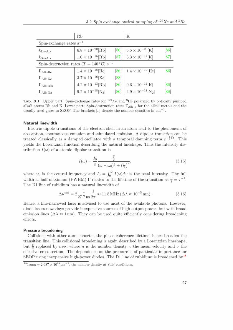
Tab. 3.1: Upper part: Spin-exchange rates for 129Xe and 3He polarized by optically pumpedalkali atoms Rb and K. Lower part: Spin-destruction rates ΓAlk−i for the alkali metals and theusually used gases in SEOP. The brackets [..] denote the number densities in cm−3.
Natural linewidthElectric dipole transitions of the electron shell in an atom lead to the phenomena of
absorption, spontaneous emission and stimulated emission. A dipolar transition can betreated classically as a damped oscillator with a temporal damping term e−
12Γt. This
yields the Lorentzian function describing the natural lineshape. Thus the intensity dis-tribution I(ω) of a atomic dipolar transition is
I(ω) =I0π
Γ2
(ω − ω0)2 +(Γ2
)2 , (3.15)
where ω0 is the central frequency and I0 =∫∞
0 I(ω)dω is the total intensity. The full
width at half maximum (FWHM) Γ relates to the lifetime of the transition as Γ2 = τ−1.
The D1 line of rubidium has a natural linewidth of
∆νnat = 21
27.7 ns
1
2π≈ 11.5MHz (∆λ ≈ 10−5 nm). (3.16)
Hence, a line-narrowed laser is advised to use most of the available photons. However,diode lasers nowadays provide inexpensive sources of high output power, but with broademission lines (∆λ ≈ 1 nm). They can be used quite efficiently considering broadeningeffects.
Pressure broadeningCollisions with other atoms shorten the phase coherence lifetime, hence broaden the
transition line. This collisional broadening is again described by a Lorentzian lineshape,but Γ
2 replaced by nvσ, where n is the number density, v the mean velocity and σ theeffective cross-section. The dependence on the pressure is of particular importance forSEOP using inexpensive high-power diodes. The D1 line of rubidium is broadened by18
181 amg = 2.687 × 1019 cm−3, the number density at STP conditions.
27
3 Optimizing the parameter space for a new 129Xe EDM search
≈ 20 GHzamg (0.04 nm
amg) at 80 C for collisions with helium, xenon and nitrogen [89]. The
broadening scales with temperature as T 0.3. At optical pumping conditions of 140 Cand 4bar the pressure broadening is
∆νpress = 20GHz
amg
4bar
1 bar
273K
413K
(413K
353K
)0.3
≈ 55GHz ≫ ∆νnat (∆λ ≈ 0.1 nm), (3.17)
which significantly increases absorption of light.Other line broadening effects like Doppler broadening are very weak (∆λ ≈ 10−3 nm)
under SEOP conditions. Note, that the Zeeman splitting of the Rb 5S1/2 levels in mag-netic fields of order 1-10 mT is not resolved, as it is of order 100MHz.Predominantly, pressure broadening makes optical pumping of alkali metals much moreefficient in pumping cells containing several atmospheres of total pressure. This broad-ening of the Rb absorption line is required in the liquid xenon experiment (cf. Sec. 5)as the laser diode linewidth is ≈ 500GHz or ≈ 1 nm. However, narrowing of the laserline can additionally (or sufficiently) increase absorption even at lower pressures. In theHe-Xe EDM experiment (cf. Sec. 6) a broad emission line is narrowed to ≈ 150GHzor ≈ 0.3 nm by back-reflecting a selected wavelength off a grating to the laser cavityto increase photon absorption. In this experiment 3He and 129Xe are simultaneouslypolarized and due to the very different optimum conditions (cf. 3.1) absorption needs tobe maximized. Generally, pressure to broaden the Rb absorption line can be providedinherently by the gas to be polarized as long as spin destruction with Rb collisions canbe compensated. Hence, in SEOP of 3He the 3He itself can be at high pressure of severalatmospheres, while in SEOP of 129Xe an additional buffer gas is needed, usually 4He.
Rate model for optically pumping rubidiumThe buildup of the Rb polarization in a dense Rb vapor can be described by a rate
model as first introduced in [90] or recently used in a slightly modified way [91].Assume the populations of the groundstatesmF = ±1/2 areN+ andN−, withN++N− =1. When pumping with σ+ light (100% polarization) the rate equations are
dN±
dt= ±
(Γ
2+ γop
)N− ∓ Γ
2N+, (3.18)
where Γ =∑
[X]ΓRb-X is the total bulk spin-destruction rate mixing the 5S1/2,mJ =±1/2 states (cf. Fig. 6 and Tab. 3.1) via collisions with other gases of number density[X] and γop is the optical pumping rate. The solution to (3.18) in a optically thick Rbvapor also depends on the depth z in the cell, yielding
PRb(t, z) = N+ −N− =γop(z)
γop(z) + Γ
(1− e−(γop(z)+Γ)t
). (3.19)
Strickly speaking, a slowing down factor S needs to be included in the exponential,altering the argument to −((γop(z) + Γ)t)/S. This factor is of order 10 and accountsfor the non-zero nuclear spin of Rb, which represents a reservoir of angular momentum,that also needs to be polarized via the hyperfine coupling to the electron spin.
28
3.2 Spin exchange optical pumping of 129Xe and 3He
Optical pumping rateThe optical pumping rate is defined as the overlap of the laser intensity profile Φ(ν, z)
with the photon absorption cross-section σ(ν)
γop(z) =
∫∞
0Φ(ν, z)σ(ν)dν. (3.20)
The absorption cross-section is assumed to be a Lorentzian of (pressure-broadened) widthΓFWHM and peak cross-section σ0 = πrecfosc, with the classical electron radius re, thespeed of light c and the D1 transition oscillator strength fosc = 0.342 [84], yielding
σ(ν) =πrecfoscΓFWHM
1
1 + 4(ν − ν0)2/Γ2FWHM
. (3.21)
The photon-flux of a Gaussian laser beam can be described at the front of the pumpingcell, where Φ(ν, z) = Φ(ν) as
Φ(ν) =PL
hν0Abeamδν
√4 ln 2
πe−4 ln 2
(ν−ν0)2
δν2 , (3.22)
where PL is the laser power, Abeam the cross-sectional area of the laser and δν the FWHMof the laser spectrum.A typical value for the optical pumping rate (3.20) in a cell of 2 bar total pressure, alaser line of 1 nm width and 1 cm2 of beam cross-sectional area is γop ≈ 105 s−1 perWatt of laser power. According to Eq. (3.19) a Rb polarization of nearly 100% can beachieved if γop ≫ Γ. The most significant alkali relaxation arises from Rb-Xe collisions.In typical SEOP conditions at 140 C where [Rb] ≈ 6×1013 cm−3 (cf. Fig. A.3) and a gasmixture of 300mbar 129Xe, 100mbar N2 and 2bar of 4He, the Rb spin destruction ratesdue to Rb, Xe, N2 and 4He are 25 s−1, 2700 s−1, 23 s−1 and 69 s−1, respectively (Tab.3.1). Already at several W of laser power the condition γop ≫ Γ can be achieved. Withdiode array bars available of up to 100 W laser power even in large cells a polarizationof the Rb vapor of nearly 100% can be maintained, which is essential for high noble gaspolarization.However, at a high photon flux it is possible to operate at higher temperatures, whichspeeds up 3He polarization as more Rb is available.
3.2.2 Alkali-noble gas collisions
In SEOP the polarization of Rb electrons is transfered to the noble-gas nuclei by spin-exchange collisions. Atomic collisions are described by their cross-section σ. The char-acteristic exchange time T ex is defined as the inverse of the collision rate γ = σvn, withthe average velocity v and the atomic number density n, hence
T ex = γ−1 = (σvn)−1. (3.23)
Assuming a Maxwell-Boltzmann distribution of velocities the average is v =√
8kBTπM ,
with the reduced mass M =malkmng
malk+mng.
29
3 Optimizing the parameter space for a new 129Xe EDM search
N
N
Xe129 He3
He3Xe129
2
2
(a) (b)
Rb
RbRb
Rb
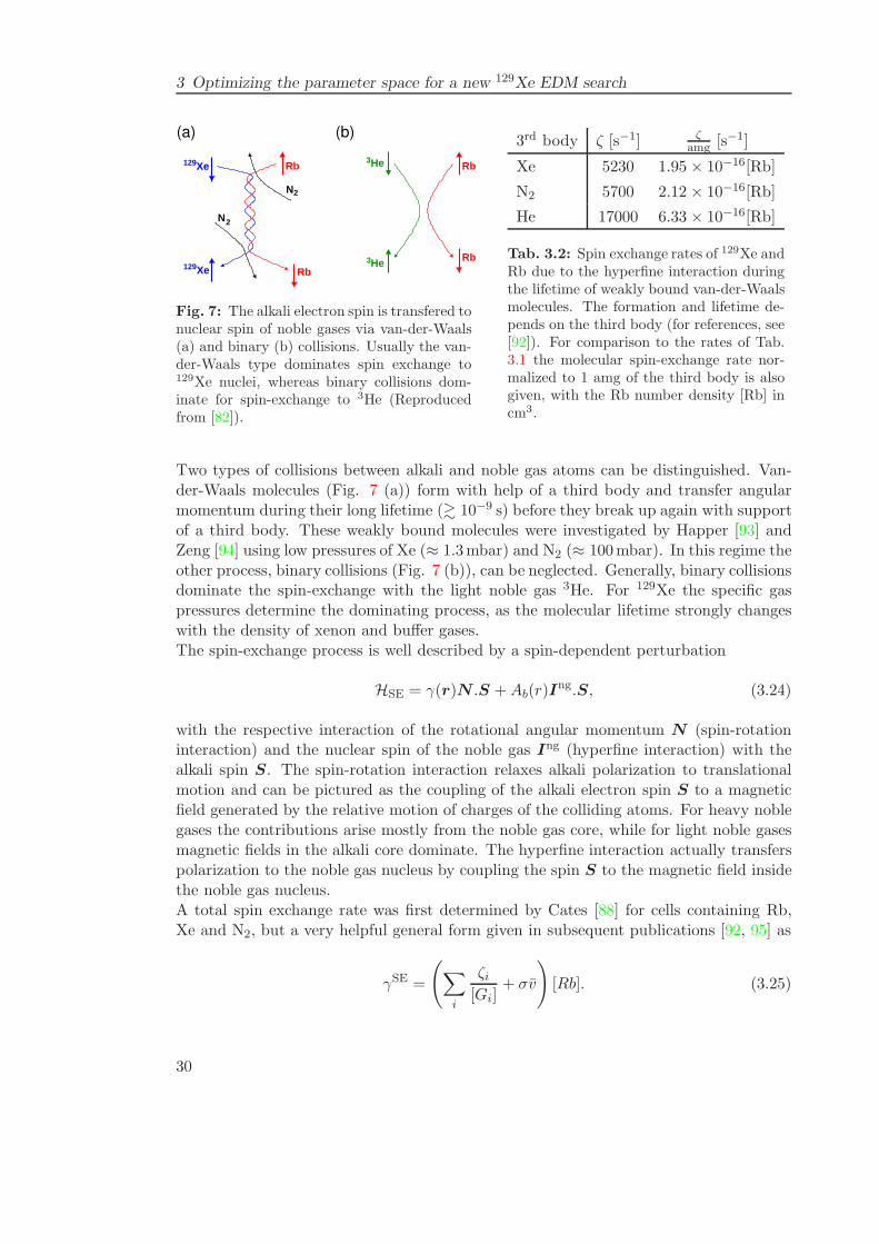
Fig. 7: The alkali electron spin is transfered tonuclear spin of noble gases via van-der-Waals(a) and binary (b) collisions. Usually the van-der-Waals type dominates spin exchange to129Xe nuclei, whereas binary collisions dom-inate for spin-exchange to 3He (Reproducedfrom [82]).
3rd body ζ [s−1] ζamg [s−1]
Xe 5230 1.95 × 10⁻¹⁶[Rb]
N2 5700 2.12 × 10⁻¹⁶[Rb]
He 17000 6.33 × 10⁻¹⁶[Rb]
Tab. 3.2: Spin exchange rates of 129Xe andRb due to the hyperfine interaction duringthe lifetime of weakly bound van-der-Waalsmolecules. The formation and lifetime de-pends on the third body (for references, see[92]). For comparison to the rates of Tab.3.1 the molecular spin-exchange rate nor-malized to 1 amg of the third body is alsogiven, with the Rb number density [Rb] incm3.
Two types of collisions between alkali and noble gas atoms can be distinguished. Van-der-Waals molecules (Fig. 7 (a)) form with help of a third body and transfer angularmomentum during their long lifetime (& 10−9 s) before they break up again with supportof a third body. These weakly bound molecules were investigated by Happer [93] andZeng [94] using low pressures of Xe (≈ 1.3mbar) and N2 (≈ 100mbar). In this regime theother process, binary collisions (Fig. 7 (b)), can be neglected. Generally, binary collisionsdominate the spin-exchange with the light noble gas 3He. For 129Xe the specific gaspressures determine the dominating process, as the molecular lifetime strongly changeswith the density of xenon and buffer gases.The spin-exchange process is well described by a spin-dependent perturbation
HSE = γ(r)N .S +Ab(r)Ing.S, (3.24)
with the respective interaction of the rotational angular momentum N (spin-rotationinteraction) and the nuclear spin of the noble gas Ing (hyperfine interaction) with thealkali spin S. The spin-rotation interaction relaxes alkali polarization to translationalmotion and can be pictured as the coupling of the alkali electron spin S to a magneticfield generated by the relative motion of charges of the colliding atoms. For heavy noblegases the contributions arise mostly from the noble gas core, while for light noble gasesmagnetic fields in the alkali core dominate. The hyperfine interaction actually transferspolarization to the noble gas nucleus by coupling the spin S to the magnetic field insidethe noble gas nucleus.A total spin exchange rate was first determined by Cates [88] for cells containing Rb,Xe and N2, but a very helpful general form given in subsequent publications [92, 95] as
γSE =
(∑
i
ζi[Gi]
+ σv
)[Rb]. (3.25)
30
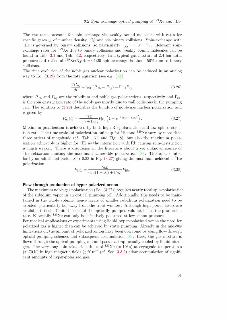
3.2 Spin exchange optical pumping of 129Xe and 3He
The two terms account for spin-exchange via weakly bound molecules with rates forspecific gases ζi of number density [Gi] and via binary collisions. Spin-exchange with3He is governed by binary collisions, so particularly γ3He
SE = σRbHev. Relevant spin-exchange rates for 129Xe due to binary collisions and weakly bound molecules can befound in Tab. 3.1 and Tab. 3.2, respectively. In a typical gas mixture of 2.4 bar totalpressure and ratios of 129Xe:N2:He=3:1:20 spin-exchange is about 50% due to binarycollisions.The time evolution of the noble gas nuclear polarization can be deduced in an analogway to Eq. (3.19) from the rate equation (see e.g. [83])
dPng
dt= γSE(PRb − Png)− ΓSDPng, (3.26)
where PRb and Png are the rubidium and noble gas polarizations, respectively and ΓSD
is the spin destruction rate of the noble gas mostly due to wall collisions in the pumpingcell. The solution to (3.26) describes the buildup of noble gas nuclear polarization andis given by
Png(t) =γSE
γSE + ΓSDPRb
(1− e−(γSE+ΓSD)t
). (3.27)
Maximum polarization is achieved by both high Rb polarization and low spin destruc-tion rate. The time scales of polarization built-up for 3He and 129Xe vary by more thanthree orders of magnitude (cf. Tab. 3.1 and Fig. 8), but also the maximum polar-ization achievable is higher for 3He as the interaction with Rb causing spin-destructionis much weaker. There is discussion in the literature about a yet unknown source of3He relaxation limiting the maximum achievable polarization [96]. This is accountedfor by an additional factor X ≈ 0.33 in Eq. (3.27) giving the maximum achievable 3Hepolarization
P3He =γSE
γSE(1 +X) + ΓSDPRb. (3.28)
Flow-through production of hyper-polarized xenonThe maximum noble gas polarization (Eq. (3.27)) requires nearly total spin-polarization
of the rubidium vapor in an optical pumping cell. Additionally, this needs to be main-tained in the whole volume, hence layers of smaller rubidium polarization need to beavoided, particularly far away from the front window. Although high power lasers areavailable this still limits the size of the optically pumped volume, hence the productionrate. Especially 129Xe can only be effectively polarized at low xenon pressures.For medical applications or experiments using liquid hyper-polarized xenon the need forpolarized gas is higher than can be achieved by static pumping. Already in the mid-90slimitations on the amount of polarized xenon have been overcome by using flow-throughoptical pumping schemes and subsequent accumulation [95]. Here, the gas mixture isflown through the optical pumping cell and passes a trap, usually cooled by liquid nitro-gen. The very long spin-relaxation times of 129Xe (≈ 104 s) at cryogenic temperatures(≈ 70K) in high magnetic fields & 20mT (cf. Sec. 3.3.2) allow accumulation of signifi-cant amounts of hyper-polarized gas.
31
3 Optimizing the parameter space for a new 129Xe EDM search
0
10
20
30
40
50
60
100
101
102
103
104
105
106
De
gre
e o
f p
ola
riza
tio
n [
%]
Time [s]
3 He
129 Xe
Fig. 8: Typical time-dependent buildup of 3He and 129Xe polarization plotted according to therate model (Eq. (3.27) and Eq. (3.28)). For spin-exchange rates see Tab. 3.1. Spin-destructionrates are deduced from typical T1 times, e.g. 100 h and 60 s for 3He and 129Xe, respectively.The variation of spin-exchange rates of 3He and 129Xe with Rb of more than three orders ofmagnitude impose experimental subtleties in realizing a repetitive clock-comparison experiment.
The remaining polarization PXe after accumulation in a cold trap for a time tacc is [95]
PXe(tacc) = PXe(0)T1tacc
(1− e−tacc/T1
), (3.29)
with the polarization leaving the optical pumping cell PXe(0) and the longitudinal re-laxation time T1 in the trap.
3.3 Relaxation mechanisms of polarized 129Xe and 3He
Longitudinal relaxation is due to the tendency of the spin system to (re-)establish ther-mal equilibrium by repopulation of the Zeeman levels. In SEOP the polarizations gen-erated are orders of magnitude larger than the thermal polarization (Eq. (3.8)). Theenergy transfer to the surrounding (or lattice) is induced by stimulated emission19. Theprocesses causing de-excitation by time varying magnetic fields or electric field gradientsare [76] relaxation at (para)magnetic impurities, spin-rotation interactions, dipole-dipoleinteractions, scalar relaxation of first and second kind, quadrupolar relaxation due toelectric field gradients and relaxation due to the chemical shift. Additionally, the longi-tudinal relaxation can also be due to diffusion in magnetic field gradients [97].Transverse relaxation is caused by dephasing of spins precessing in locally varying mag-netic fields. These field deviations can be due to close-by spins (T2) and external field
gradients (T grad2 ). Both are included in the experimentally relevant
1
T ∗2
=1
T2+
1
T grad2
(3.30)
19The probability of spontaneous emission is negligibly small at the energy separations considered.
32
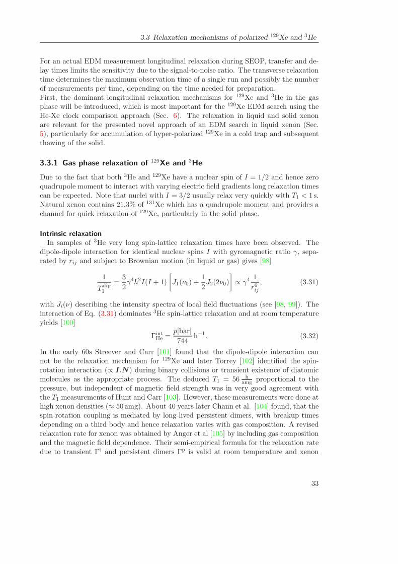
3.3 Relaxation mechanisms of polarized 129Xe and 3He
For an actual EDM measurement longitudinal relaxation during SEOP, transfer and de-lay times limits the sensitivity due to the signal-to-noise ratio. The transverse relaxationtime determines the maximum observation time of a single run and possibly the numberof measurements per time, depending on the time needed for preparation.First, the dominant longitudinal relaxation mechanisms for 129Xe and 3He in the gasphase will be introduced, which is most important for the 129Xe EDM search using theHe-Xe clock comparison approach (Sec. 6). The relaxation in liquid and solid xenonare relevant for the presented novel approach of an EDM search in liquid xenon (Sec.5), particularly for accumulation of hyper-polarized 129Xe in a cold trap and subsequentthawing of the solid.
3.3.1 Gas phase relaxation of 129Xe and 3He
Due to the fact that both 3He and 129Xe have a nuclear spin of I = 1/2 and hence zeroquadrupole moment to interact with varying electric field gradients long relaxation timescan be expected. Note that nuclei with I = 3/2 usually relax very quickly with T1 < 1 s.Natural xenon contains 21,3% of 131Xe which has a quadrupole moment and provides achannel for quick relaxation of 129Xe, particularly in the solid phase.
Intrinsic relaxationIn samples of 3He very long spin-lattice relaxation times have been observed. The
dipole-dipole interaction for identical nuclear spins I with gyromagnetic ratio γ, sepa-rated by rij and subject to Brownian motion (in liquid or gas) gives [98]
1
T dip1
=3
2γ4~2I(I + 1)
[J1(ν0) +
1
2J2(2ν0)
]∝ γ4
1
r6ij, (3.31)
with Ji(ν) describing the intensity spectra of local field fluctuations (see [98, 99]). Theinteraction of Eq. (3.31) dominates 3He spin-lattice relaxation and at room temperatureyields [100]
ΓintHe =
p[bar]
744h−1. (3.32)
In the early 60s Streever and Carr [101] found that the dipole-dipole interaction cannot be the relaxation mechanism for 129Xe and later Torrey [102] identified the spin-rotation interaction (∝ I.N) during binary collisions or transient existence of diatomicmolecules as the appropriate process. The deduced T1 = 56 h
amg proportional to thepressure, but independent of magnetic field strength was in very good agreement withthe T1 measurements of Hunt and Carr [103]. However, these measurements were done athigh xenon densities (≈ 50 amg). About 40 years later Chann et al. [104] found, that thespin-rotation coupling is mediated by long-lived persistent dimers, with breakup timesdepending on a third body and hence relaxation varies with gas composition. A revisedrelaxation rate for xenon was obtained by Anger et al [105] by including gas compositionand the magnetic field dependence. Their semi-empirical formula for the relaxation ratedue to transient Γt and persistent dimers Γp is valid at room temperature and xenon
33
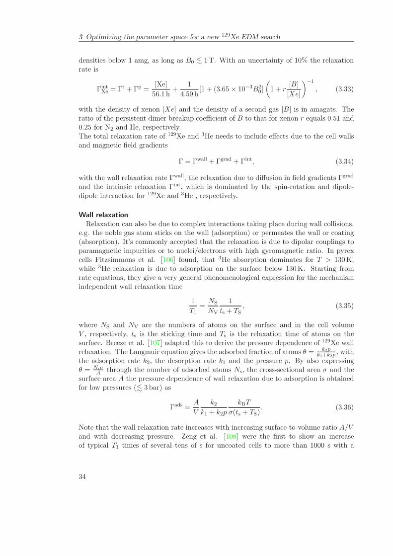
3 Optimizing the parameter space for a new 129Xe EDM search
densities below 1 amg, as long as B0 . 1T. With an uncertainty of 10% the relaxationrate is
ΓintXe = Γt + Γp =
[Xe]
56.1 h+
1
4.59 h[1 + (3.65 × 10⁻³B2
0 ]
(1 + r
[B]
[Xe]
)−1
, (3.33)
with the density of xenon [Xe] and the density of a second gas [B] is in amagats. Theratio of the persistent dimer breakup coefficient of B to that for xenon r equals 0.51 and0.25 for N2 and He, respectively.The total relaxation rate of 129Xe and 3He needs to include effects due to the cell wallsand magnetic field gradients
Γ = Γwall + Γgrad + Γint, (3.34)
with the wall relaxation rate Γwall, the relaxation due to diffusion in field gradients Γgrad
and the intrinsic relaxation Γint, which is dominated by the spin-rotation and dipole-dipole interaction for 129Xe and 3He , respectively.
Wall relaxationRelaxation can also be due to complex interactions taking place during wall collisions,
e.g. the noble gas atom sticks on the wall (adsorption) or permeates the wall or coating(absorption). It’s commonly accepted that the relaxation is due to dipolar couplings toparamagnetic impurities or to nuclei/electrons with high gyromagnetic ratio. In pyrexcells Fitzsimmons et al. [106] found, that 3He absorption dominates for T > 130K,while 3He relaxation is due to adsorption on the surface below 130K. Starting fromrate equations, they give a very general phenomenological expression for the mechanismindependent wall relaxation time
1
T1=NS
NV
1
ts + TS, (3.35)
where NS and NV are the numbers of atoms on the surface and in the cell volumeV , respectively, ts is the sticking time and Ts is the relaxation time of atoms on thesurface. Breeze et al. [107] adapted this to derive the pressure dependence of 129Xe wallrelaxation. The Langmuir equation gives the adsorbed fraction of atoms θ = k2p
k1+k2p, with
the adsorption rate k2, the desorption rate k1 and the pressure p. By also expressingθ = Nsσ
A through the number of adsorbed atoms Ns, the cross-sectional area σ and thesurface area A the pressure dependence of wall relaxation due to adsorption is obtainedfor low pressures (. 3 bar) as
Γads =A
V
k2k1 + k2p
kBT
σ(ts + TS). (3.36)
Note that the wall relaxation rate increases with increasing surface-to-volume ratio A/Vand with decreasing pressure. Zeng et al. [108] were the first to show an increaseof typical T1 times of several tens of s for uncoated cells to more than 1000 s with a
34
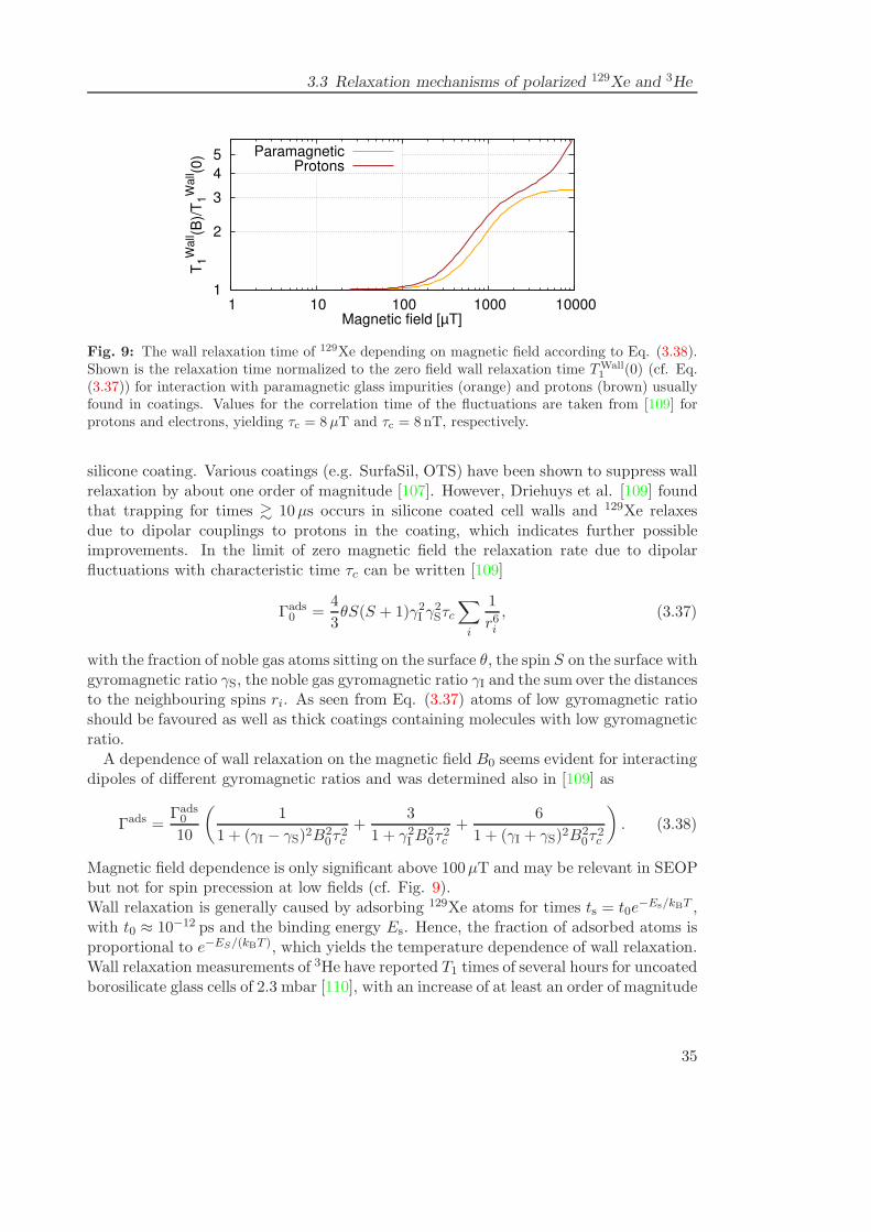
3.3 Relaxation mechanisms of polarized 129Xe and 3He
1
2
3
4
5
1 10 100 1000 10000
T1
Wa
ll (B)/
T1
Wa
ll (0)
Magnetic field [µT]
ParamagneticProtons
Fig. 9: The wall relaxation time of 129Xe depending on magnetic field according to Eq. (3.38).Shown is the relaxation time normalized to the zero field wall relaxation time TWall
1 (0) (cf. Eq.(3.37)) for interaction with paramagnetic glass impurities (orange) and protons (brown) usuallyfound in coatings. Values for the correlation time of the fluctuations are taken from [109] forprotons and electrons, yielding τc = 8µT and τc = 8nT, respectively.
silicone coating. Various coatings (e.g. SurfaSil, OTS) have been shown to suppress wallrelaxation by about one order of magnitude [107]. However, Driehuys et al. [109] foundthat trapping for times & 10µs occurs in silicone coated cell walls and 129Xe relaxesdue to dipolar couplings to protons in the coating, which indicates further possibleimprovements. In the limit of zero magnetic field the relaxation rate due to dipolarfluctuations with characteristic time τc can be written [109]
Γads0 =
4
3θS(S + 1)γ2I γ
2Sτc∑
i
1
r6i, (3.37)
with the fraction of noble gas atoms sitting on the surface θ, the spin S on the surface withgyromagnetic ratio γS, the noble gas gyromagnetic ratio γI and the sum over the distancesto the neighbouring spins ri. As seen from Eq. (3.37) atoms of low gyromagnetic ratioshould be favoured as well as thick coatings containing molecules with low gyromagneticratio.
A dependence of wall relaxation on the magnetic field B0 seems evident for interactingdipoles of different gyromagnetic ratios and was determined also in [109] as
Γads =Γads0
10
(1
1 + (γI − γS)2B20τ
2c
+3
1 + γ2IB20τ
2c
+6
1 + (γI + γS)2B20τ
2c
). (3.38)
Magnetic field dependence is only significant above 100µT and may be relevant in SEOPbut not for spin precession at low fields (cf. Fig. 9).Wall relaxation is generally caused by adsorbing 129Xe atoms for times ts = t0e
−Es/kBT ,with t0 ≈ 10−12 ps and the binding energy Es. Hence, the fraction of adsorbed atoms isproportional to e−ES/(kBT ), which yields the temperature dependence of wall relaxation.Wall relaxation measurements of 3He have reported T1 times of several hours for uncoatedborosilicate glass cells of 2.3 mbar [110], with an increase of at least an order of magnitude
35
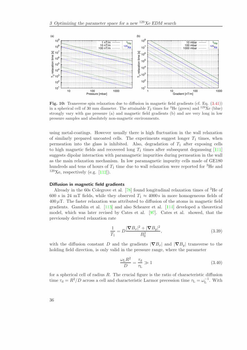
3 Optimizing the parameter space for a new 129Xe EDM search
101
102
103
104
105
106
107
108
109
10 100 1000
T2 r
ela
xa
tio
n t
ime
[s]
Pressure [mbar]
(a)
1 nT/m10 nT/m
100 nT/m
3He
129Xe
101
102
103
104
105
106
107
108
1 10 100 1000
T2 r
ela
xa
tio
n t
ime
[s]
Gradient [nT/m]
(b)
10 mbar100 mbar
1000 mbar
3He
129Xe
Fig. 10: Transverse spin relaxation due to diffusion in magnetic field gradients (cf. Eq. (3.41))in a spherical cell of 30 mm diameter. The attainable T2 times for 3He (green) and 129Xe (blue)strongly vary with gas pressure (a) and magnetic field gradients (b) and are very long in lowpressure samples and absolutely non-magnetic environments.
using metal-coatings. However usually there is high fluctuation in the wall relaxationof similarly prepared uncoated cells. The experiments suggest longer T1 times, whenpermeation into the glass is inhibited. Also, degradation of T1 after exposing cellsto high magnetic fields and recovered long T1 times after subsequent degaussing [111]suggests dipolar interaction with paramagnetic impurities during permeation in the wallas the main relaxation mechanism. In low paramagnetic impurity cells made of GE180hundreds and tens of hours of T1 time due to wall relaxation were reported for 3He and129Xe, respectively (e.g. [112]).
Diffusion in magnetic field gradientsAlready in the 60s Colegrove et al. [78] found longitudinal relaxation times of 3He of
600 s in 24 mT fields, while they observed T1 ≈ 4000 s in more homogeneous fields of400µT. The faster relaxation was attributed to diffusion of the atoms in magnetic fieldgradients. Gamblin et al. [113] and also Schearer et al. [114] developed a theoreticalmodel, which was later revised by Cates et al. [97]. Cates et al. showed, that thepreviously derived relaxation rate
1
T1= D
|∇Bx|2 + |∇By|2B2
0
, (3.39)
with the diffusion constant D and the gradients |∇Bx| and |∇By| transverse to theholding field direction, is only valid in the pressure range, where the parameter
ωLR2
D=τdτL
≫ 1 (3.40)
for a spherical cell of radius R. The crucial figure is the ratio of characteristic diffusiontime τd = R2/D across a cell and characteristic Larmor precession time τL = ω−1
L . With
36
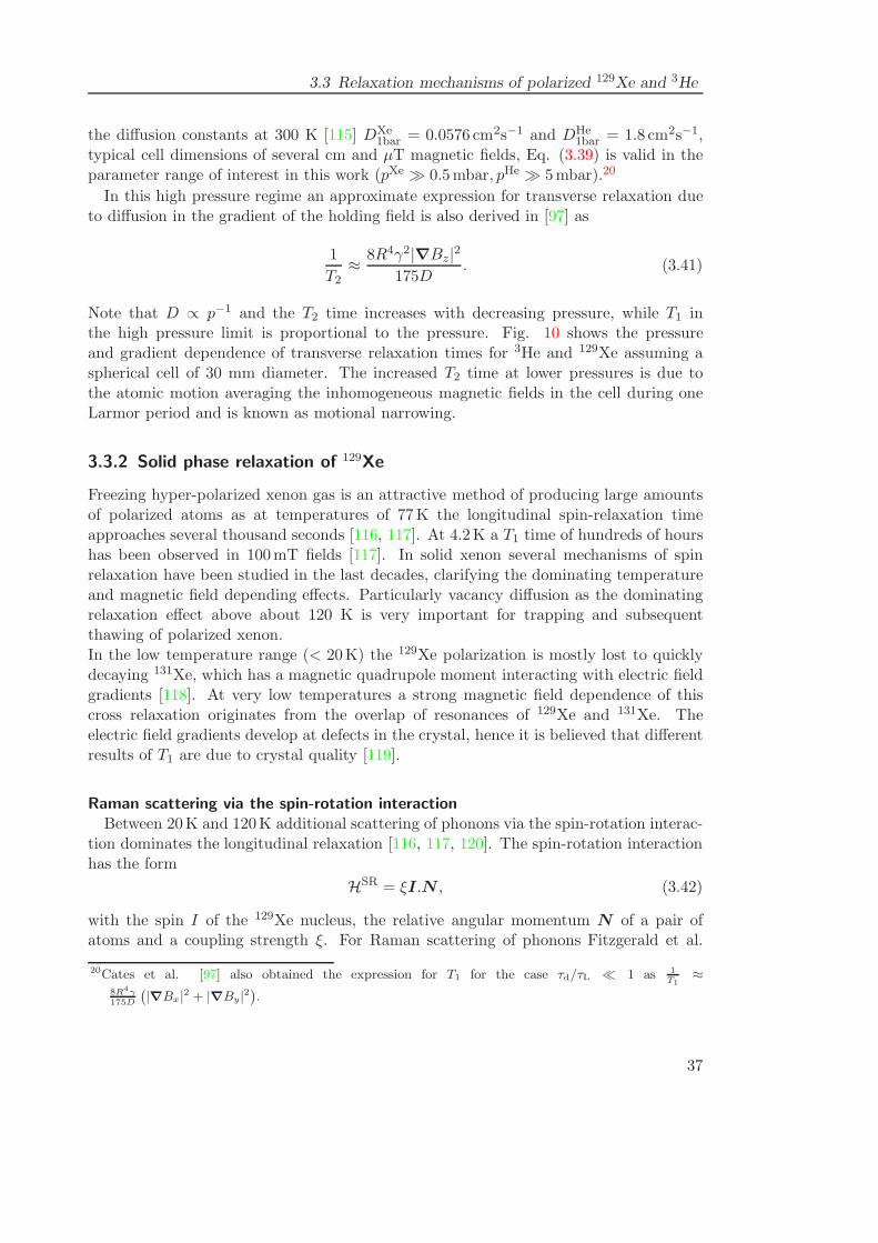
3.3 Relaxation mechanisms of polarized 129Xe and 3He
the diffusion constants at 300 K [115] DXe1bar = 0.0576 cm2s−1 and DHe
1bar = 1.8 cm2s−1,typical cell dimensions of several cm and µT magnetic fields, Eq. (3.39) is valid in theparameter range of interest in this work (pXe ≫ 0.5mbar, pHe ≫ 5mbar).20
In this high pressure regime an approximate expression for transverse relaxation dueto diffusion in the gradient of the holding field is also derived in [97] as
1
T2≈ 8R4γ2|∇Bz|2
175D. (3.41)
Note that D ∝ p−1 and the T2 time increases with decreasing pressure, while T1 inthe high pressure limit is proportional to the pressure. Fig. 10 shows the pressureand gradient dependence of transverse relaxation times for 3He and 129Xe assuming aspherical cell of 30 mm diameter. The increased T2 time at lower pressures is due tothe atomic motion averaging the inhomogeneous magnetic fields in the cell during oneLarmor period and is known as motional narrowing.
3.3.2 Solid phase relaxation of 129Xe
Freezing hyper-polarized xenon gas is an attractive method of producing large amountsof polarized atoms as at temperatures of 77K the longitudinal spin-relaxation timeapproaches several thousand seconds [116, 117]. At 4.2K a T1 time of hundreds of hourshas been observed in 100mT fields [117]. In solid xenon several mechanisms of spinrelaxation have been studied in the last decades, clarifying the dominating temperatureand magnetic field depending effects. Particularly vacancy diffusion as the dominatingrelaxation effect above about 120 K is very important for trapping and subsequentthawing of polarized xenon.In the low temperature range (< 20K) the 129Xe polarization is mostly lost to quicklydecaying 131Xe, which has a magnetic quadrupole moment interacting with electric fieldgradients [118]. At very low temperatures a strong magnetic field dependence of thiscross relaxation originates from the overlap of resonances of 129Xe and 131Xe. Theelectric field gradients develop at defects in the crystal, hence it is believed that differentresults of T1 are due to crystal quality [119].
Raman scattering via the spin-rotation interactionBetween 20K and 120K additional scattering of phonons via the spin-rotation interac-
tion dominates the longitudinal relaxation [116, 117, 120]. The spin-rotation interactionhas the form
HSR = ξI.N , (3.42)
with the spin I of the 129Xe nucleus, the relative angular momentum N of a pair ofatoms and a coupling strength ξ. For Raman scattering of phonons Fitzgerald et al.
20Cates et al. [97] also obtained the expression for T1 for the case τd/τL ≪ 1 as 1T1
≈8R4γ175D
(
|∇Bx|2 + |∇By|2)
.
37
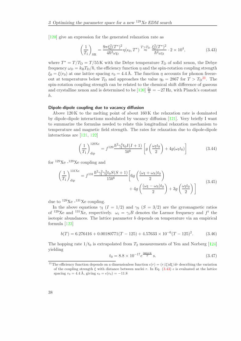
3 Optimizing the parameter space for a new 129Xe EDM search
[120] give an expression for the generated relaxation rate as
(1
T1
)
SR
=9πξ20(T
∗)2
4~2ωDη(ǫ0, T
∗)T>TD≈ ξ20(T
∗)2
~2ωD· 2× 104, (3.43)
where T ∗ = T/TD = T/55K with the Debye temperature TD of solid xenon, the Debyefrequency ωD = kBTD/~, the efficiency function η and the spin-rotation coupling strengthξ0 = ξ(r0) at one lattice spacing r0 = 4.4 A. The function η accounts for phonon freeze-out at temperatures below TD and approaches the value η0 = 2867 for T > TD
21. Thespin-rotation coupling strength can be related to the chemical shift difference of gaseousand crystalline xenon and is determined to be [120] ξ0
h = −27Hz, with Planck’s constanth.
Dipole-dipole coupling due to vacancy diffusionAbove 120K to the melting point of about 160K the relaxation rate is dominated
by dipole-dipole interactions modulated by vacancy diffusion [121]. Very briefly I wantto summarize the formulas needed to relate this longitudinal relaxation mechanism totemperature and magnetic field strength. The rates for relaxation due to dipole-dipoleinteractions are [121, 122]
(1
T1
)129Xe
dip
= f129~2γ4I t0I(I + 1)
5b6
[g
(ωIt02
)+ 4g(ωIt0)
](3.44)
for 129Xe -129Xe coupling and
(1
T1
)131Xe
dip
= f131~2γ2I γ
2St0S(S + 1)
15b6
[6g
((ωI + ωS)t0
2
)
+ 4g
((ωI − ωS)t0
2
)+ 3g
(ωIt02
)] (3.45)
due to 129Xe -131Xe coupling.
In the above equations γI (I = 1/2) and γS (S = 3/2) are the gyromagnetic ratiosof 129Xe and 131Xe, respectively. ωi = γiB denotes the Larmor frequency and f i theisotopic abundances. The lattice parameter b depends on temperature via an empiricalformula [123]
b(T ) = 6.276416 + 0.00180771(T − 125) + 4.57633 × 10⁻⁶(T − 125)2. (3.46)
The hopping rate 1/t0 is extrapolated from T2 measurements of Yen and Norberg [124]yielding
t0 = 8.8× 10⁻¹⁷e3604 K
T s. (3.47)
21The efficiency function depends on a dimensionless function ǫ(r) = (r/ξ)dξ/dr describing the variationof the coupling strength ξ with distance between nuclei r. In Eq. (3.43) ǫ is evaluated at the latticespacing r0 = 4.4 A, giving ǫ0 = ǫ(r0) = −11.8
38
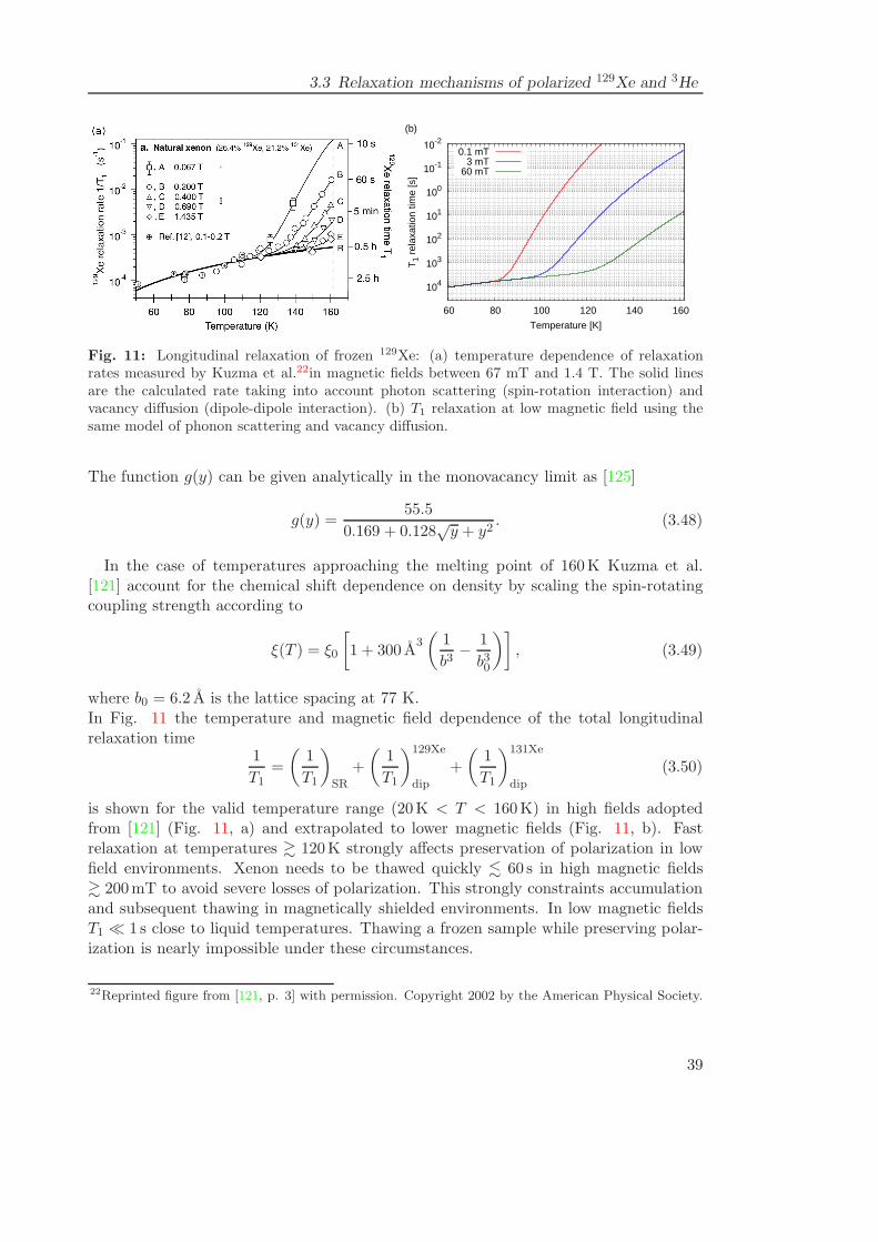
3.3 Relaxation mechanisms of polarized 129Xe and 3He
10-2
10-1
100
101
102
103
104
60 80 100 120 140 160
T1
rela
xatio
n tim
e [s
]
Temperature [K]
(b)
0.1 mT3 mT
60 mT
Fig. 11: Longitudinal relaxation of frozen 129Xe: (a) temperature dependence of relaxationrates measured by Kuzma et al.22in magnetic fields between 67 mT and 1.4 T. The solid linesare the calculated rate taking into account photon scattering (spin-rotation interaction) andvacancy diffusion (dipole-dipole interaction). (b) T1 relaxation at low magnetic field using thesame model of phonon scattering and vacancy diffusion.
The function g(y) can be given analytically in the monovacancy limit as [125]
g(y) =55.5
0.169 + 0.128√y + y2
. (3.48)
In the case of temperatures approaching the melting point of 160K Kuzma et al.[121] account for the chemical shift dependence on density by scaling the spin-rotatingcoupling strength according to
ξ(T ) = ξ0
[1 + 300 A
3(
1
b3− 1
b30
)], (3.49)
where b0 = 6.2 A is the lattice spacing at 77 K.In Fig. 11 the temperature and magnetic field dependence of the total longitudinalrelaxation time
1
T1=
(1
T1
)
SR
+
(1
T1
)129Xe
dip
+
(1
T1
)131Xe
dip
(3.50)
is shown for the valid temperature range (20K < T < 160K) in high fields adoptedfrom [121] (Fig. 11, a) and extrapolated to lower magnetic fields (Fig. 11, b). Fastrelaxation at temperatures & 120K strongly affects preservation of polarization in lowfield environments. Xenon needs to be thawed quickly . 60 s in high magnetic fields& 200mT to avoid severe losses of polarization. This strongly constraints accumulationand subsequent thawing in magnetically shielded environments. In low magnetic fieldsT1 ≪ 1 s close to liquid temperatures. Thawing a frozen sample while preserving polar-ization is nearly impossible under these circumstances.
22Reprinted figure from [121, p. 3] with permission. Copyright 2002 by the American Physical Society.
39
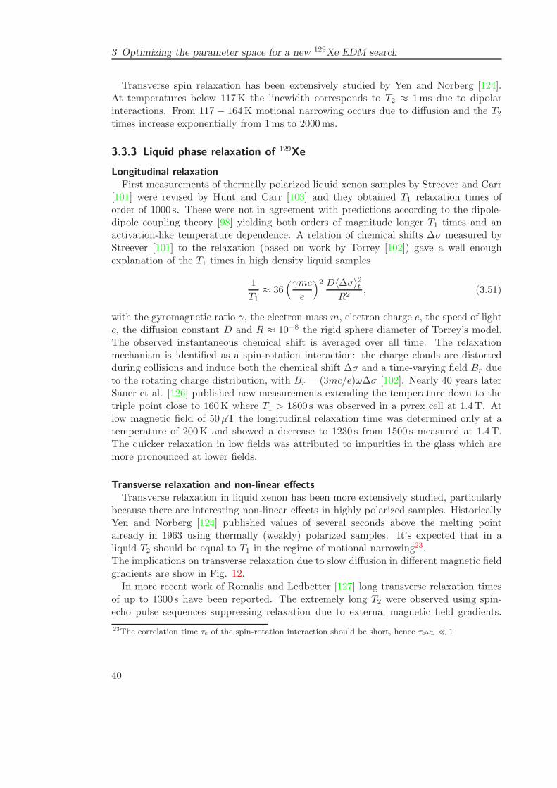
3 Optimizing the parameter space for a new 129Xe EDM search
Transverse spin relaxation has been extensively studied by Yen and Norberg [124].At temperatures below 117K the linewidth corresponds to T2 ≈ 1ms due to dipolarinteractions. From 117 − 164K motional narrowing occurs due to diffusion and the T2times increase exponentially from 1ms to 2000ms.
3.3.3 Liquid phase relaxation of 129Xe
Longitudinal relaxationFirst measurements of thermally polarized liquid xenon samples by Streever and Carr
[101] were revised by Hunt and Carr [103] and they obtained T1 relaxation times oforder of 1000 s. These were not in agreement with predictions according to the dipole-dipole coupling theory [98] yielding both orders of magnitude longer T1 times and anactivation-like temperature dependence. A relation of chemical shifts ∆σ measured byStreever [101] to the relaxation (based on work by Torrey [102]) gave a well enoughexplanation of the T1 times in high density liquid samples
1
T1≈ 36
(γmce
)2 D〈∆σ〉2tR2
, (3.51)
with the gyromagnetic ratio γ, the electron mass m, electron charge e, the speed of lightc, the diffusion constant D and R ≈ 10−8 the rigid sphere diameter of Torrey’s model.The observed instantaneous chemical shift is averaged over all time. The relaxationmechanism is identified as a spin-rotation interaction: the charge clouds are distortedduring collisions and induce both the chemical shift ∆σ and a time-varying field Br dueto the rotating charge distribution, with Br = (3mc/e)ω∆σ [102]. Nearly 40 years laterSauer et al. [126] published new measurements extending the temperature down to thetriple point close to 160K where T1 > 1800 s was observed in a pyrex cell at 1.4T. Atlow magnetic field of 50µT the longitudinal relaxation time was determined only at atemperature of 200K and showed a decrease to 1230 s from 1500 s measured at 1.4T.The quicker relaxation in low fields was attributed to impurities in the glass which aremore pronounced at lower fields.
Transverse relaxation and non-linear effectsTransverse relaxation in liquid xenon has been more extensively studied, particularly
because there are interesting non-linear effects in highly polarized samples. HistoricallyYen and Norberg [124] published values of several seconds above the melting pointalready in 1963 using thermally (weakly) polarized samples. It’s expected that in aliquid T2 should be equal to T1 in the regime of motional narrowing23.The implications on transverse relaxation due to slow diffusion in different magnetic fieldgradients are show in Fig. 12.
In more recent work of Romalis and Ledbetter [127] long transverse relaxation timesof up to 1300 s have been reported. The extremely long T2 were observed using spin-echo pulse sequences suppressing relaxation due to external magnetic field gradients.
23The correlation time τc of the spin-rotation interaction should be short, hence τcωL ≪ 1
40
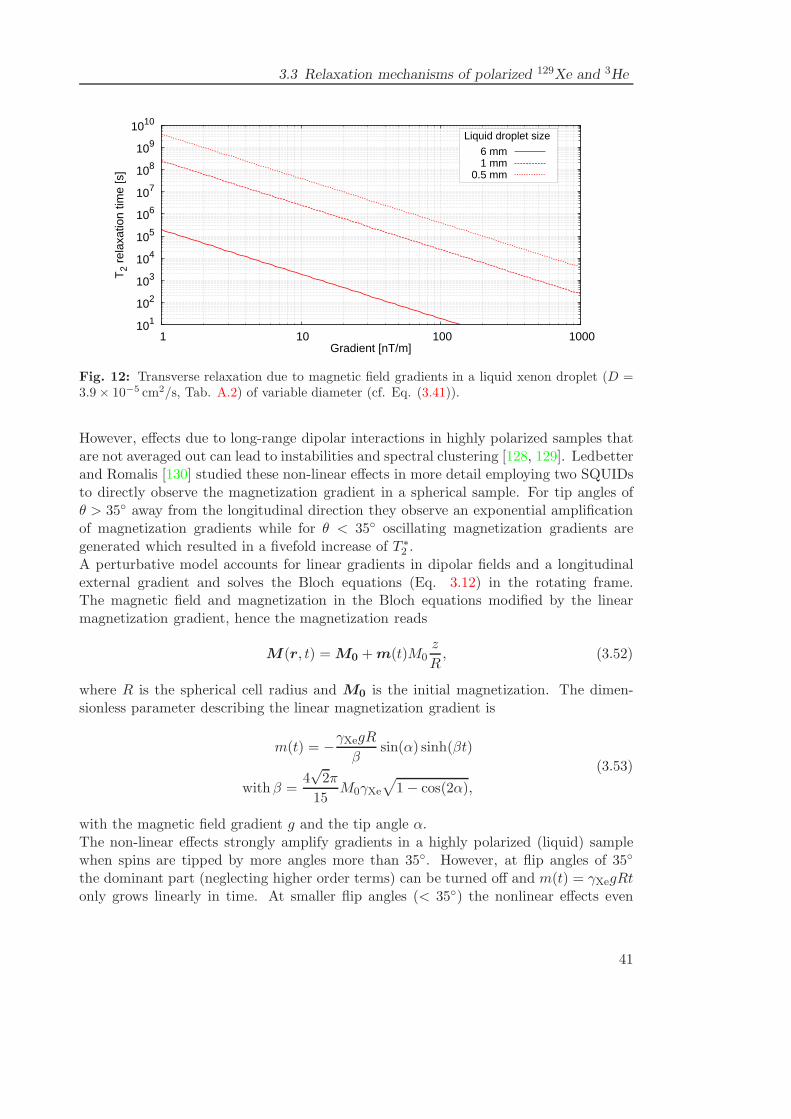
3.3 Relaxation mechanisms of polarized 129Xe and 3He
101
102
103
104
105
106
107
108
109
1010
1 10 100 1000
T2
rela
xatio
n tim
e [s
]
Gradient [nT/m]
Liquid droplet size
6 mm1 mm
0.5 mm
Fig. 12: Transverse relaxation due to magnetic field gradients in a liquid xenon droplet (D =3.9× 10⁻⁵ cm2/s, Tab. A.2) of variable diameter (cf. Eq. (3.41)).
However, effects due to long-range dipolar interactions in highly polarized samples thatare not averaged out can lead to instabilities and spectral clustering [128, 129]. Ledbetterand Romalis [130] studied these non-linear effects in more detail employing two SQUIDsto directly observe the magnetization gradient in a spherical sample. For tip angles ofθ > 35 away from the longitudinal direction they observe an exponential amplificationof magnetization gradients while for θ < 35 oscillating magnetization gradients aregenerated which resulted in a fivefold increase of T ∗
2 .A perturbative model accounts for linear gradients in dipolar fields and a longitudinalexternal gradient and solves the Bloch equations (Eq. 3.12) in the rotating frame.The magnetic field and magnetization in the Bloch equations modified by the linearmagnetization gradient, hence the magnetization reads
M(r, t) = M0 +m(t)M0z
R, (3.52)
where R is the spherical cell radius and M0 is the initial magnetization. The dimen-sionless parameter describing the linear magnetization gradient is
m(t) = −γXegR
βsin(α) sinh(βt)
with β =4√2π
15M0γXe
√1− cos(2α),
(3.53)
with the magnetic field gradient g and the tip angle α.The non-linear effects strongly amplify gradients in a highly polarized (liquid) samplewhen spins are tipped by more angles more than 35. However, at flip angles of 35
the dominant part (neglecting higher order terms) can be turned off and m(t) = γXegRtonly grows linearly in time. At smaller flip angles (< 35) the nonlinear effects even
41
3 Optimizing the parameter space for a new 129Xe EDM search
suppress the growth of the magnetization gradients and lead to spectral narrowing.The non-linear effects basically depend on the ambient external gradient, the sample sizeand sample magnetization and their implications on the liquid xenon EDM measurementneed to be studied under existing experimental conditions.
3.4 SQUID detection
A highly sensitive detection of nuclear spin precession is a main challenge in atomicEDM experiments, as the ratio of observed signal to detection noise is substantiallydetermining the EDM senstivity (cf. Sec. 4.2). Optical detection of spin precessionhas been employed in the 199Hg EDM measurement [67, 131] giving an intrinsicallyvery low noise level. In a search for a 129Xe EDM optical detection is not as straightforward and currently not the preferred detection technique. However, EDM searchesare currently planned with an improved spin maser concept. The 129Xe precession isdetected via optical absorption of 794.8 nm light in a rubidium vapor due to a smalltransverse magnetization of 129Xe [132]. The drawback here is, that the rubidium vaporin the EDM cell potentially limits the breakdown voltage and causes unwanted frequencyshifts. Nevertheless, an improvement of the noise level due to optical detection can stillincrease the EDM sensitivity.In the efforts presented in this work the precessing nuclear spins in very low magneticfields are detected using SQUIDs. SQUIDs provide a very sensitive probe of magneticflux changes as the intrinsic noise density of commercially available SQUID sensors is onthe order of several fT/
√Hz even at frequencies down to a few Hz. Reviews of SQUIDs
and applications can be found in [133, 134] and the comprehensive SQUID handbook[135]. Operation of SQUIDs is based on the phenomena of superconductivity presentedin various textbooks, e.g. [136, 137].
3.4.1 Superconductivity and the Josephson effect
In the superconducting state single electron scattering is eliminated as phonon exchangebetween two electrons leads to an attractive long-range interaction. The paired elec-trons, called Cooper pairs, have opposite spins, hence they are subject to Bose-Einsteinstatistics and tend to occupy a single ground state. The distance of two weakly boundelectrons is specified by the coherence length ζ ≈ 100 nm, which is much larger thanthe average cooper pair distance r = 1nm. The strong overlap of the wave-functionsallows a phase-coherent description of the superconducting state by a single many-bodywave-function
Ψ(r) = |Ψ(r)|eiϕ(r). (3.54)
To break up a Cooper pair and create two quasi-particle excitations an energy of 2∆ ≈10−3 eV is necessary, which can be added thermally (critical temperature Tc), kinetically(critical current jc) or magnetically (critical fieldHc). As the binding of the Cooper pairsestablishes an energy gap ∆ at the Fermi level, the lack of available electron states makesthe electron pairs propagate unscattered. This phenomenon of superconductivity brings
42
3.4 SQUID detection
along several new effects, like flux expulsion in superconductors (Meissner effect) [138],flux quantization (Φ0 = 2.068 × 10⁻¹⁵ Wb, 1Wb = 1Tm2) or the Josephson effect[139], particularly important for understanding the operational principle of SQUIDs andexplained in the following.In 1962 Josephson predicted a supercurrent arising from Cooper pairs tunneling througha weak link between two superconductors, that can be a insulating or normal conductinglayer of thickness d ≪ ζ. Assume the two superconductors on either side of the weaklink are described by two wave-functions Ψ1 = |Ψ1|eiϕ1 and Ψ2 = |Ψ2|eiϕ2 . Then thegauge invariant phase difference reads
∆ϕ = ϕ2 − ϕ1 −2π
φ0
∫Adl. (3.55)
The first Josephson relation (Feynman [140] gives a derivation for the case withoutmagnetic fields, A = 0) relates the supercurrent Is at zero voltage difference to thephase difference ∆ϕ as
Is = Ic sin∆ϕ, (3.56)
where Ic is the critical current determined by the weak link, typically of order 102 −104 A/cm2. The second Josephson relation arises from the time-derivative of the phasedifference ∆ϕ as
d∆ϕ
dt=
2e
~V =
2π
Φ0V, (3.57)
with the fluxoid Φ0 = h2e and the voltage difference V across the junction. For a con-
stant potential across the junction V 6= 0 the supercurrent (3.56) starts oscillating at afrequency ν = 2eV
h , typically in the GHz range.
3.4.2 SQUIDs and the flux-locked loop
With Josephson junctions in superconducting loops an extremely sensitive flux to voltageconverter can be set up making use of interference of the coherent wave-functions24.Assume a magnetic flux Φa penetrates the loop and two Josephson junctions J1, J2link the input and output terminals of the SQUID device (Fig. 13). The two wave-functions traveling across different Josephson junctions interfere at the output terminal.A magnetic flux Φa through the SQUID loop causes a circular current Icir differentlyaffecting the phase changes at the two Josephson junctions. Hence the interference ofboth wave-functions yields a modulation of the maximum supercurrent according to themagnetic flux. The resulting pattern is well known from two-slit interference in opticsand can be derived with the Josephson equations.Integration of the wave vector k = mv−qA
~along a circular closed path within the loop
(dashed line in Fig. 13) yields a relation between the flux Φa =∮Adl through the loop
24In a dc SQUID two Josephson junctions are used and the device can be directly read out electronically,while rf SQUIDs use only on junction, but need a tank circuit for read out. Rf SQUIDs were not ofinterest in this work as they usually have less sensitivity.
43
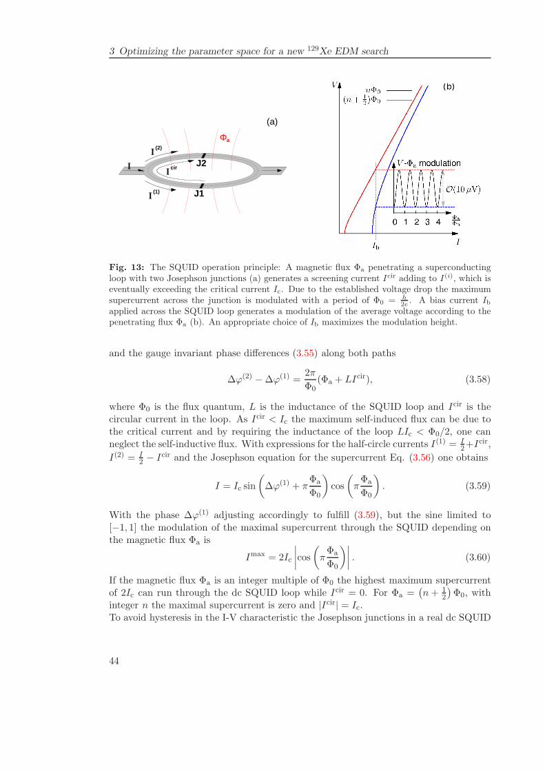
3 Optimizing the parameter space for a new 129Xe EDM search
Φa
(1)I
(2)I
I
J1
J2cirI
(a)
Fig. 13: The SQUID operation principle: A magnetic flux Φa penetrating a superconductingloop with two Josephson junctions (a) generates a screening current Icir adding to I(i), which iseventually exceeding the critical current Ic. Due to the established voltage drop the maximumsupercurrent across the junction is modulated with a period of Φ0 = h
2e . A bias current Ibapplied across the SQUID loop generates a modulation of the average voltage according to thepenetrating flux Φa (b). An appropriate choice of Ib maximizes the modulation height.
and the gauge invariant phase differences (3.55) along both paths
∆ϕ(2) −∆ϕ(1) =2π
Φ0(Φa + LIcir), (3.58)
where Φ0 is the flux quantum, L is the inductance of the SQUID loop and Icir is thecircular current in the loop. As Icir < Ic the maximum self-induced flux can be due tothe critical current and by requiring the inductance of the loop LIc < Φ0/2, one canneglect the self-inductive flux. With expressions for the half-circle currents I(1) = I
2+Icir,
I(2) = I2 − Icir and the Josephson equation for the supercurrent Eq. (3.56) one obtains
I = Ic sin
(∆ϕ(1) + π
Φa
Φ0
)cos
(πΦa
Φ0
). (3.59)
With the phase ∆ϕ(1) adjusting accordingly to fulfill (3.59), but the sine limited to[−1, 1] the modulation of the maximal supercurrent through the SQUID depending onthe magnetic flux Φa is
Imax = 2Ic
∣∣∣∣cos(πΦa
Φ0
)∣∣∣∣ . (3.60)
If the magnetic flux Φa is an integer multiple of Φ0 the highest maximum supercurrentof 2Ic can run through the dc SQUID loop while Icir = 0. For Φa =
(n+ 1
2
)Φ0, with
integer n the maximal supercurrent is zero and |Icir| = Ic.To avoid hysteresis in the I-V characteristic the Josephson junctions in a real dc SQUID
44
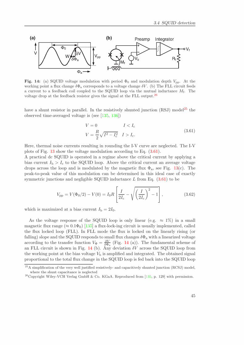
3.4 SQUID detection
Fig. 14: (a) SQUID voltage modulation with period Φ0 and modulation depth Vpp. At theworking point a flux change δΦa corresponds to a voltage change δV . (b) The FLL circuit feedsa current to a feedback coil coupled to the SQUID loop via the mutual inductance Mf. Thevoltage drop at the feedback resistor gives the signal at the FLL output.26
have a shunt resistor in parallel. In the resistively shunted junction (RSJ) model25 theobserved time-averaged voltage is (see [135, 136])
V = 0 I < Ic
V =R
2
√I2 − I2c I > Ic.
(3.61)
Here, thermal noise currents resulting in rounding the I-V curve are neglected. The I-Vplots of Fig. 13 show the voltage modulation according to Eq. (3.61).A practical dc SQUID is operated in a regime above the critical current by applying abias current Ib > Ic to the SQUID loop. Above the critical current an average voltagedrops across the loop and is modulated by the magnetic flux Φa, see Fig. 13(c). Thepeak-to-peak value of this modulation can be determined in this ideal case of exactlysymmetric junctions and negligible SQUID inductance L from Eq. (3.61) to be
Vpp = V (Φ0/2)− V (0) = I0R
I
2Ic−
√(I
2Ic
)2
− 1
, (3.62)
which is maximized at a bias current Ib = 2I0.
As the voltage response of the SQUID loop is only linear (e.g. ≈ 1%) in a smallmagnetic flux range (≈ 0.1Φ0) [135] a flux-lock-ing circuit is usually implemented, calledthe flux locked loop (FLL). In FLL mode the flux is locked on the linearly rising (orfalling) slope and the SQUID responds to small flux changes δΦa with a linearized voltageaccording to the transfer function VΦ = ∂V
∂Φa(Fig. 14 (a)). The fundamental scheme of
an FLL circuit is shown in Fig. 14 (b). Any deviation δV across the SQUID loop fromthe working point at the bias voltage Vb is amplified and integrated. The obtained signalproportional to the total flux change in the SQUID loop is fed back into the SQUID loop
25A simplification of the very well justified resistively- and capacitively shunted junction (RCSJ) model,where the shunt capacitance is neglected
26Copyright Wiley-VCH Verlag GmbH & Co. KGaA. Reproduced from [135, p. 129] with permission.
45
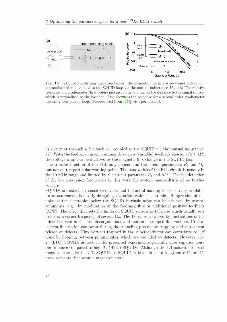
3 Optimizing the parameter space for a new 129Xe EDM search
superconducting shield
I
Φ
Lin
Min
SQUID
pickup coil
(a)
Fig. 15: (a) Superconducting flux transformer: the magnetic flux in a wire-wound pickup coilis transformed and coupled to the SQUID loop via the mutual inductance Min. (b) The relativeresponse of a gradiometer (first order) pickup coil depending on the distance to the signal source,which is normalized to the baseline. Also shown is the response for a second order gradiometerfeaturing four pickup loops (Reproduced from [134] with permission).
as a current through a feedback coil coupled to the SQUID via the mutual inductanceMf. With the feedback current running through a (variable) feedback resistor (Rf ≈ kΩ)the voltage drop can be digitized as the magnetic flux change in the SQUID loop.The transfer function of the FLL only depends on the circuit parameters Rf and Mf,but not on the particular working point. The bandwidth of the FLL circuit is usually inthe 10 MHz range and limited by the circuit parameter Rf and Mf
27. For the detectionof the low precession frequencies in this work the system bandwidth is of no furtherconcern.SQUIDs are extremely sensitive devices and the art of making the sensitivity availablefor measurements is mostly designing low noise readout electronics. Suppression of thenoise of the electronics below the SQUID intrinsic noise can be achieved by severaltechniques, e.g. by modulation of the feedback flux or additional positive feedback(APF). The effect that sets the limits on SQUID sensors is 1/f noise which usually setsin below a corner frequency of several Hz. The 1/f noise is caused by fluctuations of thecritical current in the Josephson junctions and motion of trapped flux vortices. Criticalcurrent fluctuation can occur during the tunneling process by trapping and subsequentrelease at defects. Flux vortices trapped in the superconductor can contribute to 1/fnoise by hopping between pinning sites, which are provided by defects. However, lowTc (LTC) SQUIDs as used in the presented experiments generally offer superior noiseperformance compared to high Tc (HTC) SQUIDs. Although the 1/f noise is orders ofmagnitude smaller in LTC SQUIDs, a SQUID is less suited for longterm drift or DCmeasurements than atomic magnetometers.
46
3.4 SQUID detection
3.4.3 Practical SQUID magnetometers and gradiometers
The SQUID loop is rarely well suited for magnetic field measurements. The energy reso-lution of a resistively shunted dc SQUID under optimum conditions is ǫ(f) ≈ 16kBT
√LC
[135], hence a SQUID loop should have very small inductance and capacitance. A smallinductance corresponds to a small enclosed area, typically AL < 10−2 mm2. Athough,the SQUID is extremely flux sensitive ≈ 10−6 Φ0, the field sensitivity δB = δΦ/AL turnsout to be orders of magnitude worse. To overcome this a washer of large outer diameterD and very small hole d can be used to increase the effective area to Aeff = dD by focus-ing the field. Another now widely used approach is implementation of a multi-turn fluxtransformer. A superconducting pickup coil of experimentally favourable dimensions andturns picks up the magnetic flux, which is transformed to an input coil on the SQUIDchip. The input coil is coupled to the SQUID loop via the mutual inductance Min, seeFig. 15 (a). This gives the freedom of having the pickup coil on chip or have it self-madeusing niobium wire. In the latter case the coil can be external of a superconductingshield, which encloses the SQUID chip. The only constrain on the external pickup coilis matching it’s inductance to the inductance of the input coil, usually hundreds of nHto some µH. The inductance of a (flat) superconducting loop is given by [134]
L = µ0N2rcoil
[ln
(8rcoilrwire
)− 2
], (3.63)
with the number of turns N , the radius of the coil rcoil and the radius of the wire rwire.For high magnetic flux sensitivity a large coil area is preferred. However, it is constrainedexperimentally by it’s size, by the anticipated spatial resolution and the intrinsic mag-netic field noise of the SQUID. Additionally, to benefit from a large pickup loop area theenvironmental magnetic field noise has to be lower than the loop sensitivity. A rule ofthumb is the coil diameter should be at least the distance to the source.In the detectionof nearby signal sources external niobium wire pickup coils are particularly helpful as thegradiometer configuration can greatly reduce the noise level. From the 1/r3 dependenceof the fields the optimum baseline of a gradiometer can be determined (Fig. 15 (b)).
27The bandwidth can be estimated by f3dB ≈ VΦMf
Rf
·GBP , where VΦMf
Rf
is the SQUID gain and GBPis the gain bandwidth product set in the SQUID software, typically 0.23GHz.
47

4 Improving EDM measurements of 129Xe
As already pointed out (Eq. (2.29)) the signature of an EDM in “conventional” searchesis a shift of the Larmor frequency due to a coupling of the EDM to an additionally appliedelectric field. The source of a frequency shift δν 6= 0 can not easily be disentangled. In ameasurement with electric field of E = 10kV/cm and assuming an EDM d = 10−26 ecmthe obtained frequency shift δν is
δν =2(δd)E
h≈ 4× 10⁻⁸ Hz, (4.1)
with Planck’s constant h. The same shift is generated by a magnetic field variation δBof order
δB =h(δν)
2µ≈ 10−15 T, (4.2)
where the magnetic moment µ ≈ 4× 10⁻²⁷ J/T.To account for this in the analysis a lot of effort needs to be put in precise monitoringof the magnetic field during an EDM measurement with parallel fields. Sensitivitycan mostly be enhanced by (further) tuning of experimental parameters and a betterunderstanding of systematic effects. To overcome general limitations of the parallel fieldsmethod new approaches are highly motivated.In this chapter I will first discuss the experiment from which the most recent EDM limiton 129Xe was obtained and the fundamental parameters determining the sensitivity ofan EDM search. The section will be concluded by adressing possible improvements inparallel fields EDM searches in the gas phase and new concepts.
4.1 Background
For the isotope 129Xe the most recent limit from an experiment at the University ofMichigan [71] was measured with a spin-maser setup. The method allows observation ofspin precession for arbitrarily long times not being limited by spin relaxation times. Nextto 129Xe a second species (3He) in the EDM cell provides extremely useful informationon magnetic field variations. The limit for 129Xe that was determined with the spinmaser technique is dXe = 0.7± 3.3 · 10−27 ecm.
The two maser species are polarized in a pumping cell by SEOP using Rb metal andconstantly diffuse to the cylindrical EDM cell (Fig. 16). The spins in a gas mixtureof 85mbar 129Xe , 860mbar 3He and 62mbar of nitrogen precess in a magnetic field of315µT inside a magnetically shielded environment. The rotating magnetization inducescurrents in resonant circuits consisting of pickup coils and capacitors (CHe and CXe).
49
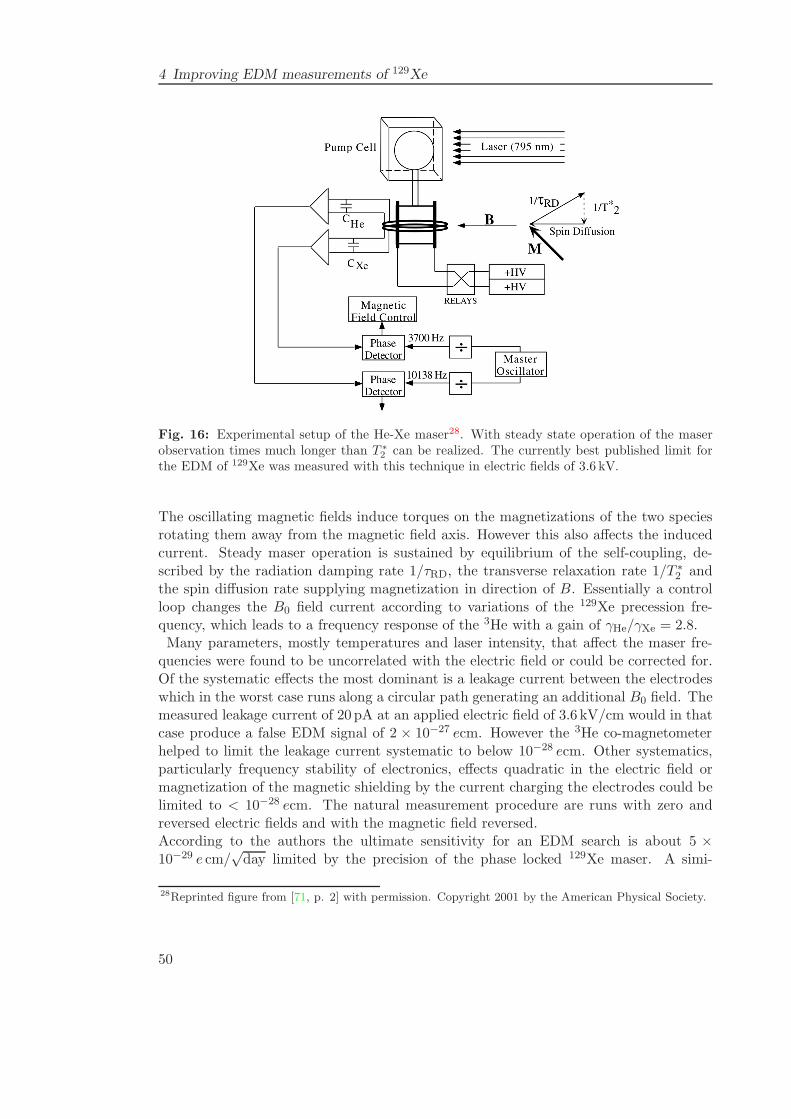
4 Improving EDM measurements of 129Xe
Fig. 16: Experimental setup of the He-Xe maser28. With steady state operation of the maserobservation times much longer than T ∗
2 can be realized. The currently best published limit forthe EDM of 129Xe was measured with this technique in electric fields of 3.6 kV.
The oscillating magnetic fields induce torques on the magnetizations of the two speciesrotating them away from the magnetic field axis. However this also affects the inducedcurrent. Steady maser operation is sustained by equilibrium of the self-coupling, de-scribed by the radiation damping rate 1/τRD, the transverse relaxation rate 1/T ∗
2 andthe spin diffusion rate supplying magnetization in direction of B. Essentially a controlloop changes the B0 field current according to variations of the 129Xe precession fre-quency, which leads to a frequency response of the 3He with a gain of γHe/γXe = 2.8.Many parameters, mostly temperatures and laser intensity, that affect the maser fre-
quencies were found to be uncorrelated with the electric field or could be corrected for.Of the systematic effects the most dominant is a leakage current between the electrodeswhich in the worst case runs along a circular path generating an additional B0 field. Themeasured leakage current of 20 pA at an applied electric field of 3.6 kV/cm would in thatcase produce a false EDM signal of 2 × 10⁻²⁷ ecm. However the 3He co-magnetometerhelped to limit the leakage current systematic to below 10−28 ecm. Other systematics,particularly frequency stability of electronics, effects quadratic in the electric field ormagnetization of the magnetic shielding by the current charging the electrodes could belimited to < 10−28 ecm. The natural measurement procedure are runs with zero andreversed electric fields and with the magnetic field reversed.According to the authors the ultimate sensitivity for an EDM search is about 5 ×10⁻²⁹ e cm/
√day limited by the precision of the phase locked 129Xe maser. A simi-
28Reprinted figure from [71, p. 2] with permission. Copyright 2001 by the American Physical Society.
50
4.2 Fundamental limitations
lar maser technique improved by optical detection of the precession is planned to beused in a 129Xe EDM search in Japan. The sensitivity to frequency measurements basedon observed spin precession without electric field is quoted differently by the same groupas ≈ 10−31 ecm within 10 days [141] and ≈ 10−28 ecm within 10000 s [142].
4.2 Fundamental limitations
In the following the sensitivity of the EDM d will be deduced depending on the relevantexperimental parameters. Systematic effects are assumed to be zero, e.g. the magneticfield is known exactly or generally µ.B is known much better than d.E.The fundamental uncertainty of a measurement of a single spin frequency running for along time τ can be given according to Heisenberg’s energy-time uncertainty principle as~(δω)τ = ~ and hence
δω =1
τ(4.3)
Assume the measurement is repeated N times at a signal-to-noise ratio S/n, then29
δω =1
τ(S/n)√N
=ǫ√fBW
τS√N, (4.4)
with the noise density ǫ and the bandwidth fBW. The number of measurements in a totalmeasurement time T is N = T/τ and the bandwidth can be assumed as fBW ≈ 1/τ .With Eq. (2.29) the fundamental sensitivity of an EDM determined from the uncertaintyin the frequency measurement is
σd =~
2E
ǫ
τ3/2S√N
=~
2E
ǫ
τS√T. (4.5)
The above derivation yields a very similar estimate as the frequency sensitivity accordingto the Cramer-Rao lower bound for an exponentiall decaying sine wave , see eg. [112].
4.2.1 Methods to improve EDM sensitivity
The fundamental sensitivity (Eq. (4.5)) reveals the obvious ways to go for an improvedEDM limit.Polar molecules are highly polarizable and hence offer very high internal electric fields ofseveral tens of GV/cm in moderate laboratory fields, while EDM searches on particlesand atoms are technically limited to tens of kV/cm. Several searches for the electronEDM with molecules (e.g. YbF, PbO, ThO,...) are currently on the way. Very recentlythe limit on the electron EDM has been improved to < 9 × 10⁻²⁹ ecm [69] using themolecule ThO.An increase in signal size corresponds to a higher density sample, e.g. high spin polariza-tion. For EDM searches using particles or atomic/molecular beams an increase in signal
29The noise is assumed to be white noise.
51
4 Improving EDM measurements of 129Xe
size is not straightforward and limited by available facilities and upgrade progress. EDMsearches with polarized noble gases are basically free to choose a gas density as desired.However, there is a trade off as the observation time τ of freely precessing spins, whichin that case is T ∗
2 , is inversely proportional to the density.In particular a long observation time significantly improves the sensitivity, which isharder to achieve by slowing atomic/molecular beams or by trapping of atoms in cav-ities. For the very promising radioactive isotopes with octupole deformation this isadditionally limited by their lifetime, but for radium and radon this is sufficiently longτ1/2 > 1000 s.The noise density ǫ of the background also needs to be reduced for an enhanced sensitiv-ity. Detection using a low-noise sensor is a challenging encounter, as the measurementsare preferably done at very low frequencies of tens of Hz. The 199Hg EDM experimentbenefits from optical detection of the spin precession and quotes [131] a measured rootmean square (rms) noise density of 30µV. At a typical signal amplitude of 3 V thisresults in a signal-to-noise ratio of 3× 10⁴ (inferring a bandwidth of fBW ≈ 10Hz). Be-sides potentially useful atomic magnetometers with demonstrated sub-fT noise density[143] SQUIDs provide a relatively easy to use highly sensitive sensor for magnetic flux.The magnetic flux noise density of LTc SQUIDs is as low as . 2 fT/
√Hz for frequen-
cies down to several Hz. The possibility of using external superconducting pickup coilsoffers a variety of geometric shapes including gradiometer designs. A typical EDM cellwith tens of mbar of 129Xe polarized at 10% yields some nT magnetic flux in a few cmdistance. Assuming only intrinsic SQUID noise, a signal-to-noise ratio of ≈ 105 − 106 isexpected, potentially at least an order of magnitude better than the currently availableoptical detection technique.
4.2.2 An improved conventional EDM search
Several EDM experiments try to exploit the fundamental sensitivity of Eq. (4.5) byfurther improving the established method of parallel electric and magnetic fields. Thesystematics are mostly well-known and new results can be obtained with moderate ef-fort. However, the gain in sensitivity is less significant.An effort of an EDM search using 129Xe in a gas phase sample and using parallel fieldsis described in Sec. 6. Inside a magnetically shielded room with the best possible envi-ronment in terms of magnetic field gradients, homogeneity of the residual field and verylow noise, we aim to observe 129Xe spin-precession with very little magnetic and electricdisturbance. A clock-comparison with a 3He co-magnetometer and in a later stage thecorrelation of several external magnetometers compensate for magnetic field variations.With a SQUID based low-noise detection system a large signal-to-noise ratio greatlyimproves sensitivity.The fundamental sensitivity of this approach with an applied electric field of E =10kV/cm and assuming a T ∗
2 ≈ 200 s is estimated to be (Eq. (4.5))
σd =~
2 · 10 kV/cm2 fT/
√Hz
(200 s)3/2 · 1 nT1√N
≈ 2× 10⁻²⁹ ecm√N, (4.6)
52
4.2 Fundamental limitations
with the number of measurements N .
4.2.3 Next generation EDM search in liquid 129Xe
Nevertheless the fundamental sensitivity limit is usually missed by at least an order ofmagnitude due to systematic effects. For significant progress towards new EDM limitsnew methods are strongly encouraged. Under development are EDM searches usingprotons, deuterons or muons in storage rings [144] and our novel approach aiming to useliquid hyper-polarized 129Xe and time-varying electric fields. Superconducting pickupcoils very close to the 129Xe samples connected to SQUID current sensors with intrinsicnoise < 2 fT/
√Hz sense a magnetic flux due to Larmor precession of about 10 nT (at
several % polarization). The method, setup and progress of this new effort is presentedin Sec. 5. Implementation of rotating electric fields leads to decoupling of the rotationdirections of the Larmor precession µ.B from the precession due to the term d.E, whichrelaxes magnetic field requirements and introduces totally different systematics not yetstudied. The potential gain of this approach using very small, but high density samplesis an EDM sensitivity on the order of 10−29 ecm in a single measurement, but presumablylimited by systematic effects from oscillating currents. Details on this future method ofrotating electric fields and the obtained sensitivity are discussed in Sec. 5.1.Nevertheless a parallel fields measurement has a similar fundamental sensitivity (Eq.(4.5)). Assuming E = 50kV/cm and T ∗
2 ≈ 500 s using a polarized liquid one obtains
σd =~
2 · 50 kV/cm2 fT/
√Hz
(500 s)3/2 · 10 nT1√N
≈ 1.2 × 10⁻³¹ ecm√N, (4.7)
where N again denotes the total number of measurements.The potential of an EDM search in a liquid is high, but experimentally very demanding.In this long-term effort a thorough study of a rich field of new systematic effects, theirundertanding and control is of utterly importance.
53

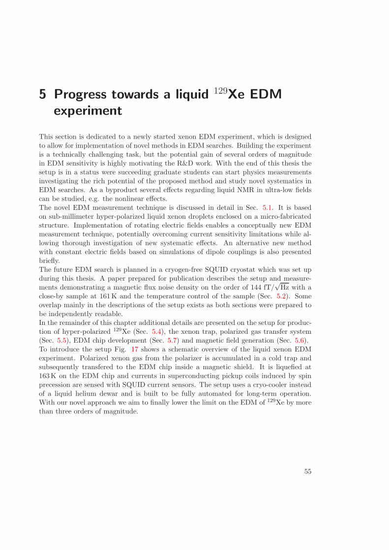
5 Progress towards a liquid 129Xe EDMexperiment
This section is dedicated to a newly started xenon EDM experiment, which is designedto allow for implementation of novel methods in EDM searches. Building the experimentis a technically challenging task, but the potential gain of several orders of magnitudein EDM sensitivity is highly motivating the R&D work. With the end of this thesis thesetup is in a status were succeeding graduate students can start physics measurementsinvestigating the rich potential of the proposed method and study novel systematics inEDM searches. As a byproduct several effects regarding liquid NMR in ultra-low fieldscan be studied, e.g. the nonlinear effects.The novel EDM measurement technique is discussed in detail in Sec. 5.1. It is basedon sub-millimeter hyper-polarized liquid xenon droplets enclosed on a micro-fabricatedstructure. Implementation of rotating electric fields enables a conceptually new EDMmeasurement technique, potentially overcoming current sensitivity limitations while al-lowing thorough investigation of new systematic effects. An alternative new methodwith constant electric fields based on simulations of dipole couplings is also presentedbriefly.The future EDM search is planned in a cryogen-free SQUID cryostat which was set upduring this thesis. A paper prepared for publication describes the setup and measure-ments demonstrating a magnetic flux noise density on the order of 144 fT/
√Hz with a
close-by sample at 161K and the temperature control of the sample (Sec. 5.2). Someoverlap mainly in the descriptions of the setup exists as both sections were prepared tobe independently readable.In the remainder of this chapter additional details are presented on the setup for produc-tion of hyper-polarized 129Xe (Sec. 5.4), the xenon trap, polarized gas transfer system(Sec. 5.5), EDM chip development (Sec. 5.7) and magnetic field generation (Sec. 5.6).To introduce the setup Fig. 17 shows a schematic overview of the liquid xenon EDMexperiment. Polarized xenon gas from the polarizer is accumulated in a cold trap andsubsequently transfered to the EDM chip inside a magnetic shield. It is liquefied at163K on the EDM chip and currents in superconducting pickup coils induced by spinprecession are sensed with SQUID current sensors. The setup uses a cryo-cooler insteadof a liquid helium dewar and is built to be fully automated for long-term operation.With our novel approach we aim to finally lower the limit on the EDM of 129Xe by morethan three orders of magnitude.
55
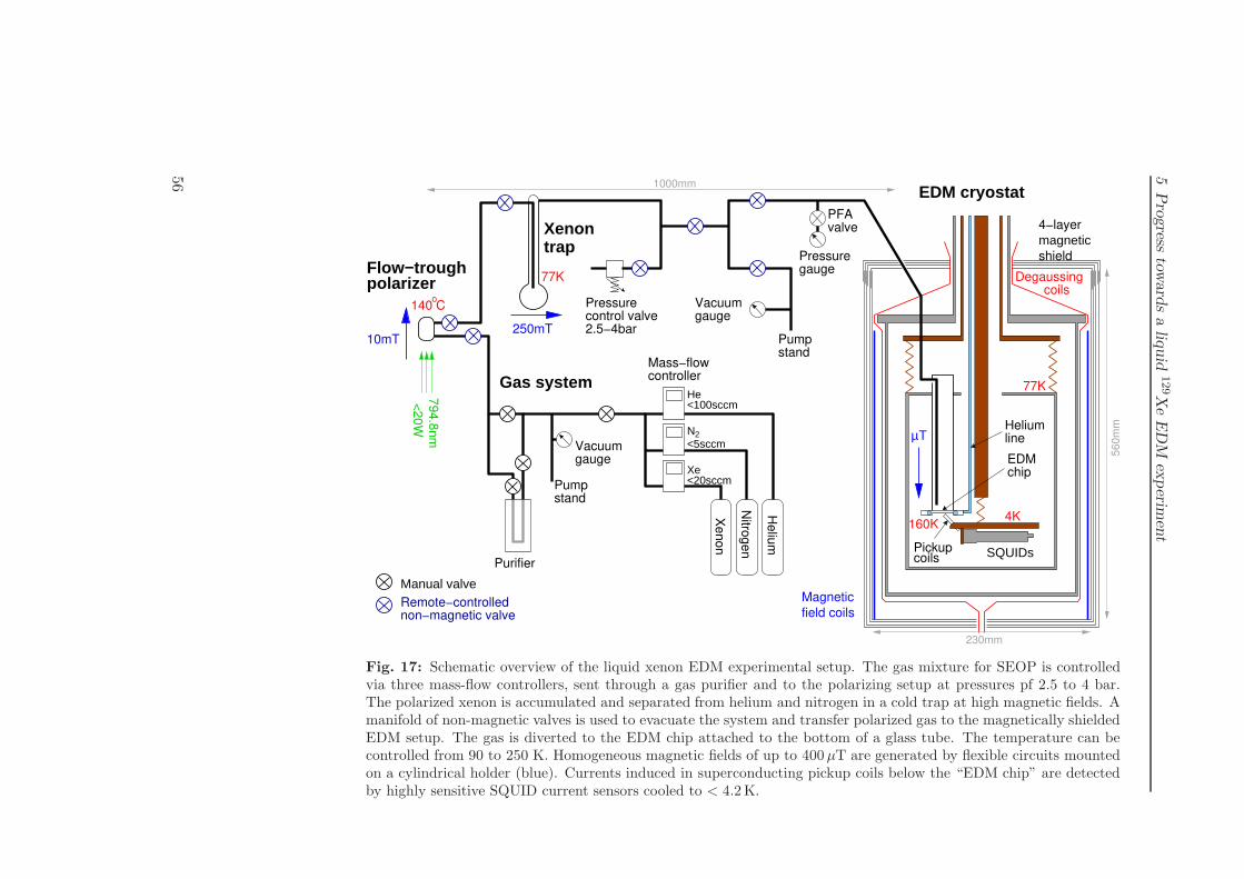
5Progress
toward
saliq
uid
129X
eEDM
experim
ent
Manual valve
He<100sccm
N<5sccm
2
Xe<20sccm
Gas system
EDM cryostat
SQUIDs
magnetic4−layer
shield
Purifier
Magnetic
field coils
Degaussingcoils
Mass−flowcontroller
coilsPickup
EDMchip
lineHelium
Pressurecontrol valve2.5−4bar
Pumpstand
gaugeVacuum
Pumpstand
Vacuumgauge
79
4.8
nm
<2
0W
Xe
no
n
Nitro
ge
n
He
lium
56
0m
m
230mm
PFA
Pressuregauge
valve
1000mm
Flow−troughpolarizer
trapXenon
Tµ
Remote−controlled non−magnetic valve
140 Co
10mT
4K
77K
160K
77K
250mT
Fig. 17: Schematic overview of the liquid xenon EDM experimental setup. The gas mixture for SEOP is controlledvia three mass-flow controllers, sent through a gas purifier and to the polarizing setup at pressures pf 2.5 to 4 bar.The polarized xenon is accumulated and separated from helium and nitrogen in a cold trap at high magnetic fields. Amanifold of non-magnetic valves is used to evacuate the system and transfer polarized gas to the magnetically shieldedEDM setup. The gas is diverted to the EDM chip attached to the bottom of a glass tube. The temperature can becontrolled from 90 to 250 K. Homogeneous magnetic fields of up to 400µT are generated by flexible circuits mountedon a cylindrical holder (blue). Currents induced in superconducting pickup coils below the “EDM chip” are detectedby highly sensitive SQUID current sensors cooled to < 4.2K.
56
5.1 A novel approach to measure the EDM of 129Xe
5.1 A novel approach to measure the EDM of 129Xe
In this section I mostly discuss the novel method of rotating electric fields we aim toimplement in the xenon EDM setup. A large part will be dedicated to systematic effectsthat need to be considered. These effects are new to EDM searches as they arise fromtime-varying electric fields and need to be studied experimentally to be well understood.
5.1.1 Different ways to search for an EDM within this approach
“Ramsey-type” EDM searchIn a typical EDM search a static electric field E is applied either parallel or anti-
parallel to a magnetic holding field B0. A deviation in Larmor precession frequency ωL
for E = 0 and E 6= 0 can be attributed to an electric dipole moment (cf. Eqn. (2.29)):
~ωL = 2(µ.B0 − d.E), (5.1)
where E can be aligned parallel and anti-parallel to B0, respectively. Using oppositepolarities of the electric field the observed change in ωL is δωL = 4Ed/~ and directlytranslates to an EDM d.This method strongly relies on highly stable (or precisely known) magnetic fields todisentangle false EDM effects due to magnetic field deviations. Accordingly, the stabilityof B0 already limits the EDM sensitivity and highly sensitive magnetic field monitoringis essential.
Rotating electric fieldsWe aim to employ a novel EDM measurement technique introducing rotating electric
fields rather than static electric fields to overcome current sensitivity limitations. In thisapproach the electric field E is applied perpendicular to B0 and co-rotating with thepolarization P at a constant phase ϕ (cf. Fig. 18). The interaction of a non-zero EDMwith the electric field causes a rotation of the polarization vector P according to P ×E
at a frequency ωd = dE/~, orthogonal to ωL. Hence, in our approach B0 fluctuations ordrifts do not cause false EDM effects and constrictions on the knowledge of B0 are lesssevere.
An EDM measurement starts by applying a highly accurate oscillating (or rotating)B1 pulse to flip the polarization P (initially aligned along B0) by an (arbitrary) angleθ1. Alternating voltages applied to eight electrodes embedded around each droplet cangenerate individually rotating electric fields. Phase-locked to the free precession signalsthe electric fields of e.g. three simultaneous experiments can be rotating (i) with a phaseϕ = π
2 , (ii) in phase ϕ = 0 and (iii) with a phase ϕ = −π2 with respect to P (cf. Fig. 18).
After a free precession period τ a second B1 pulse flips P by an angle θ2 = π−θ1. In caseof a finite permanent EDM the polarization is rotated out of the precession plane during
a free precession period τ accumulating an angle θ(i)d = ωdτ = dEτ
~= −θ(iii)d , where
θ(i)d and θ
(iii)d denote the angle in droplets with opposite electric field directions. An
accumulated phase causes a misalignment of P and B0 after the second spin-flip pulse,
57
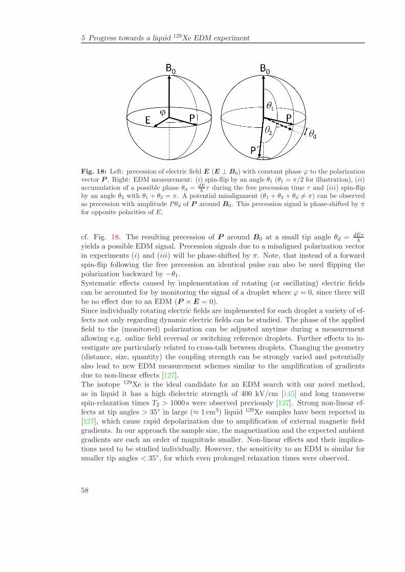
5 Progress towards a liquid 129Xe EDM experiment
Fig. 18: Left: precession of electric field E (E ⊥ B0) with constant phase ϕ to the polarizationvector P . Right: EDM measurement: (i) spin-flip by an angle θ1 (θ1 = π/2 for illustration), (ii)accumulation of a possible phase θd = dE
~τ during the free precession time τ and (iii) spin-flip
by an angle θ2 with θ1 + θ2 = π. A potential misalignment (θ1 + θ2 + θd 6= π) can be observedas precession with amplitude Pθd of P around B0. This precession signal is phase-shifted by πfor opposite polarities of E.
cf. Fig. 18. The resulting precession of P around B0 at a small tip angle θd = dEτ~
yields a possible EDM signal. Precession signals due to a misaligned polarization vectorin experiments (i) and (iii) will be phase-shifted by π. Note, that instead of a forwardspin-flip following the free precession an identical pulse can also be used flipping thepolarization backward by −θ1.Systematic effects caused by implementation of rotating (or oscillating) electric fieldscan be accounted for by monitoring the signal of a droplet where ϕ = 0, since there willbe no effect due to an EDM (P ×E = 0).Since individually rotating electric fields are implemented for each droplet a variety of ef-fects not only regarding dynamic electric fields can be studied. The phase of the appliedfield to the (monitored) polarization can be adjusted anytime during a measurementallowing e.g. online field reversal or switching reference droplets. Further effects to in-vestigate are particularly related to cross-talk between droplets. Changing the geometry(distance, size, quantity) the coupling strength can be strongly varied and potentiallyalso lead to new EDM measurement schemes similar to the amplification of gradientsdue to non-linear effects [127].The isotope 129Xe is the ideal candidate for an EDM search with our novel method,as in liquid it has a high dielectric strength of 400 kV/cm [145] and long transversespin-relaxation times T2 > 1000 s were observed previously [127]. Strong non-linear ef-fects at tip angles > 35 in large (≈ 1 cm3) liquid 129Xe samples have been reported in[127], which cause rapid depolarization due to amplification of external magnetic fieldgradients. In our approach the sample size, the magnetization and the expected ambientgradients are each an order of magnitude smaller. Non-linear effects and their implica-tions need to be studied individually. However, the sensitivity to an EDM is similar forsmaller tip angles < 35, for which even prolonged relaxation times were observed.
58
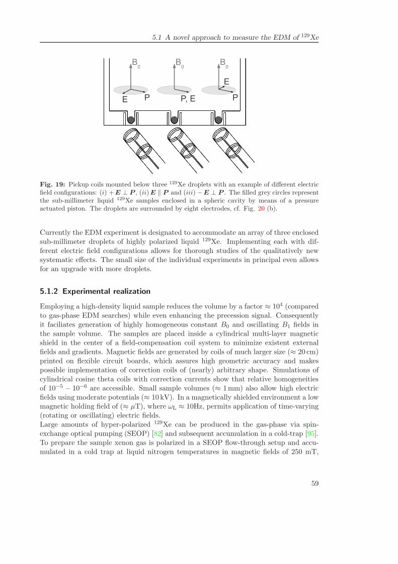
5.1 A novel approach to measure the EDM of 129Xe
Fig. 19: Pickup coils mounted below three 129Xe droplets with an example of different electricfield configurations: (i) +E ⊥ P , (ii)E ‖ P and (iii) −E ⊥ P . The filled grey circles representthe sub-millimeter liquid 129Xe samples enclosed in a spheric cavity by means of a pressureactuated piston. The droplets are surrounded by eight electrodes, cf. Fig. 20 (b).
Currently the EDM experiment is designated to accommodate an array of three enclosedsub-millimeter droplets of highly polarized liquid 129Xe. Implementing each with dif-ferent electric field configurations allows for thorough studies of the qualitatively newsystematic effects. The small size of the individual experiments in principal even allowsfor an upgrade with more droplets.
5.1.2 Experimental realization
Employing a high-density liquid sample reduces the volume by a factor ≈ 104 (comparedto gas-phase EDM searches) while even enhancing the precession signal. Consequentlyit faciliates generation of highly homogeneous constant B0 and oscillating B1 fields inthe sample volume. The samples are placed inside a cylindrical multi-layer magneticshield in the center of a field-compensation coil system to minimize existent externalfields and gradients. Magnetic fields are generated by coils of much larger size (≈ 20 cm)printed on flexible circuit boards, which assures high geometric accuracy and makespossible implementation of correction coils of (nearly) arbitrary shape. Simulations ofcylindrical cosine theta coils with correction currents show that relative homogeneitiesof 10−5 − 10−6 are accessible. Small sample volumes (≈ 1mm) also allow high electricfields using moderate potentials (≈ 10 kV). In a magnetically shielded environment a lowmagnetic holding field of (≈ µT), where ωL ≈ 10Hz, permits application of time-varying(rotating or oscillating) electric fields.Large amounts of hyper-polarized 129Xe can be produced in the gas-phase via spin-exchange optical pumping (SEOP) [82] and subsequent accumulation in a cold-trap [95].To prepare the sample xenon gas is polarized in a SEOP flow-through setup and accu-mulated in a cold trap at liquid nitrogen temperatures in magnetic fields of 250 mT,
59
5 Progress towards a liquid 129Xe EDM experiment
where longitudinal spin-relaxation is slow [117]. The maximum polarization of 400 mbarof natural xenon in a 20 cm3 cell determined by calibration with protons is ≈ 20%and builds up in about 100 s. After accumulation for about 20 min 129Xe is transferedthrough PFA and glass tubing to a glass tube of 20 mm diameter mounted in the EDMsetup. A micro-structured plate (“EDM chip”) of 35 mm diameter and 2.5 mm thick-ness made of machinable ceramics or quartz is attached to the glass tube, where thepolarized gas liquefies at ≈ 163K. The “EDM chip” is micro-structured to provide threecylindrical or (preferably) spherical cavities, aligned in a line and separated by about 5mm. A pressure actuated piston is used to encapsulate separated samples of liquifiedxenon in the embedded microstructures. Depolarization effects in this volume can beminimized by appropriate surface treatment and coatings [107, 108]. The temperatureof the “EDM chip” can be controlled between 90 K to 250 K by means of helium gas,which enables us to freeze, liquefy and evaporate xenon (161.4K < Tliquid < 165.2K).The precession of P around the B0 axis in each experiment is detected by superconduct-ing gradiometer pickup coils mounted just below the downside of the “EDM chip” andtilted at a large angle of 45 to also be sensitive to transverse fields. The gradiometersare made of twelve turns of niobium wire (Tc = 9.2K) on a 2 mm diameter sapphire rod.Magnetic induction is measured by connecting the coils to highly sensitive LTc SQUIDcurrent sensors. Both the SQUID current sensors and the niobium pickup coils are ther-mally anchored to the 4.2 K stage of a dry helium cooling machine. A vacuum gap of≈ 1mm maintains thermal insulation and an aluminum coating on the downside of the“EDM chip” reduces heat radiation from the “EDM chip”. The SQUID sensors have adesign noise level of < 2 fT/
√Hz at frequencies above 3 Hz. The Larmor frequency for
the EDM measurement can be chosen accordingly to minimize noise mostly caused bymechanical vibrations and the power line frequency (γXe = 11.777Hz/µT).
Static electric field sensitivityThe primary goal of our EDM search is to introduce the novel method of rotating
electric fields and investigation of the expected new systematic effects to determine theultimate potential of this approach. On the way the setup can be easily adapted toemploy the standard EDM measurement technique with a static electric field applied inparallel to the magnetic field. This can be accomplished by metallization of the pistonused for droplet enclosure. This layer in conjunction with the aluminum layer on thedownside of the “EDM chip” can be used to apply potentials of order 10-15 kV over 1-2mm. Hence, a liquid xenon sample (whether enclosed or not) can be exposed to electricfields of order 50 kV/cm.Most dominantly magnetic field stability and leakage currents limit “Ramsey-type” EDMsearches. Highly stable, low-noise magnetic fields of O(µT) can be generated by ultra-low noise current sources [131, 146]. Leakage currents of order 0.5 pA [67] and 20 pA[71] are considerably limiting the EDM searches using 199Hg (≈ 10−30 ecm) and of 129Xe(≈ 10−27 ecm), respectively. In an effort for a “Ramsey-type” EDM search with liquidxenon direct leakage currents through the sample and the high-resistivity “EDM chip”(> 1016 Ωcm) can be neglected. The top electrode on the piston has no direct contact
60
5.1 A novel approach to measure the EDM of 129Xe
to the glass tube and the glass is at low temperatures (< 200K). Leakage currentsfollowing helical paths along the inner glass wall are expected to be extremely small. Inthe case of a one-turn helical current of 0.01 pA (d = 18mm) along the inner wall of theglass tube, the magnetic field (≈ 0.7 × 10⁻¹⁸ T) alternating with the electric field of 50kV/cm would mimic an EDM of order 10−31 ecm (cf. Eqn. (4.2)).For false EDM effects due to accumulation of geometric phases [147] using a liquid sampleis particularly advantageous over gas phase EDM searches. Diffusion in the liquid ismany orders of magnitude slower resulting in a short mean free path and slow diffusivemotion of order ≈ 100µm/s [124]. Transverse motional magnetic fields Bm = c−2v ×E
contribute to geometric phase induced false effects but are suppressed by many ordersof magnitude in a liquid sample30.The statistical sensitivity (Eqn. (4.7)) of this “Ramsey-type” EDM search gives d ≈1.2× 10⁻³¹ ecm in a single measurement.
Rotating electric field sensitivityIn a configuration with time-varying electric fields of 50 kV
cm and a spin precession timeT2 ≈ 1000 s an EDM of d = 1.4 × 10⁻³⁰ ecm gives rise to an accumulated angle duringfree precession of
θd =dEτ
~≈ 1× 10⁻⁷. (5.2)
Keep in mind, that the angle due to the precession of the EDM in the electric field of50 kV/cm accumulates at a rate of only ≈ 10−10 s−1, which is the figure of merit usedin the systematics discussion.Arbitrarily assuming a droplet diameter of 1mm containing about 8× 10¹⁸ atoms and apolarization of 10% the precession signal amplitude at 1 mm distance of the pickup loopsat 45 is ≈ 220 nT, cf. Eqn. (6.2). The difference of signals from experiments (i) and(iii) (Fig. 19) arising from the accumulated angle θd gives the EDM signal size ≈ 40 fT.With the intrinsic noise level of the SQUID current sensors of 2 fT/
√Hz we get a signal-
to-noise ratio on the order of 10. Statistically the experiment can be repeated 104 timesin ≈ 150 days and potentially improve the statistical sensitivity to . 10−32 ecm.However many new systematics of the rotating electric field method need to be wellstudied and understood in detail. In the following section I will discuss these systematiceffects and give order of magnitude estimates of their relevance.
5.1.3 New systematic effects due to rotating electric fields
On account of the liquid sample effects of motional magnetic fields are strongly sup-pressed. The electric field is aligned normal to the B0 direction, hence systematic effectsconcerning magnetic field stability are not limiting the sensitivity as severely as in “con-ventional” EDM experiments with E ‖ B0. Although the tip angle θ1 is generallyarbitrary the droplet (ii) (Fig. 19) can be best used as a reference in the special caseof θ1 = π
2 . The signal will not show any rotation out of the precession plane due to
30The motional magnetic field contributes transverse components of order c−2 · 100 × 10−6 m/s ·50 kV/cm ≈ 5 fT.
61
5 Progress towards a liquid 129Xe EDM experiment
an EDM when E 6= 0 is co-rotating with the polarization vector (P × E = 0). Notyet studied systematic effects in regard to the time-varying electric field can be thor-oughly investigated with the reference experiment. In principal any (or several) of thethree droplets can be used as references by adjusting the electric field phases on-lineduring free precession, which offers a very versatile tool for a systematics survey. Thefollowing discussion of expected systematic effects will focus on effects introduced by thetime-varying electric fields and assume a tip angle of π/2.
Motional magnetic fieldsIn the liquid phase the 129Xe atoms are moving with velocities on the order of self-
diffusion (v ≈ 100µm/s) and therefore experience a motional magnetic field of
Bm = − 1
c2v ×E. (5.3)
The radial component vr of the atomic motion perpendicular to B0 effectively causesmodulation of the B0 field and hence the precession frequency by δωL = ±γXec
−2vrE.For E = 50kV/cm and the velocity of self diffusion this effect accounts for a modulationof δB0 ≈ 5 fT. The effect causes a frequency broadening on the 10−9 level for a 1µTholding field but no false EDM (ωL ⊥ ωd).Atoms moving with an axial component vz experience a motional magnetic field Bm,r
along the polarization vector (v ×E ‖ P ), therefore motion along the B0 axis yields noeffect P ×Bm,r = 0. These considerations assume a perfectly aligned electric field withan exact phase angle of ϕ = π/2 to the polarization vector. Let’s see what an electricfield misalignment implicates.
Electric field misalignmentFirst of all consider the case where the electric field is misaligned in the precession
plane and the phase angle between E and P is ϕ = π2 ± δϕ (cf. Fig. 20). For atoms
moving radially to B0 with vr this only causes a negligible change in the mentionedmodulation of B0 (vr ×E ‖ B0).Atoms moving in vertical direction in an electric field of E = 50kV/cm with velocityvz ≈ 100µm/s experience a motional magnetic field of order 5 fT. For a misalignment ofthe phase angle δϕ = 0.02 (≈ 1) this radial field is not parallel to P and P ×Bm,r 6= 0.The nuclear spin precesses slowly about the motional field component of size 0.1 fTaccumulating a false EDM angle at a rate of
2πγXe · 0.02 · Bm,r ≈ 10−8 s−1. (5.4)
However, the time between collisions in the liquid is on the order of τ = (σnv)−1 ≈10−5 s, where the cross-section σ is taken as roughly the square of the van-der-Waalsradius r2 = (216 pm)2 and the number density n ≈ 1022 cm−3. Between collisions anangle of θd ≈ 10−13 can be accumulated corresponding to d ≈ 10−36 ecm. Additionally,to first order the effect is expected to cancel, as electric field rotation is much fastercompared to atomic diffusion.
62
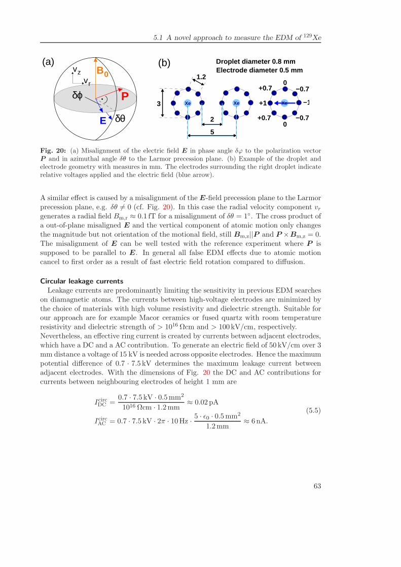
5.1 A novel approach to measure the EDM of 129Xe
B0
Pδϕ
E δθ
vzvr
(a)
5
0
0
+1 −1
−0.7
−0.7
+0.7
+0.7
Xe Xe Xe3
1.2
2
Droplet diameter 0.8 mmElectrode diameter 0.5 mm
(b)
Fig. 20: (a) Misalignment of the electric field E in phase angle δϕ to the polarization vectorP and in azimuthal angle δθ to the Larmor precession plane. (b) Example of the droplet andelectrode geometry with measures in mm. The electrodes surrounding the right droplet indicaterelative voltages applied and the electric field (blue arrow).
A similar effect is caused by a misalignment of the E-field precession plane to the Larmorprecession plane, e.g. δθ 6= 0 (cf. Fig. 20). In this case the radial velocity component vrgenerates a radial field Bm,r ≈ 0.1 fT for a misalignment of δθ = 1. The cross product ofa out-of-plane misaligned E and the vertical component of atomic motion only changesthe magnitude but not orientation of the motional field, still Bm,z||P and P ×Bm,z = 0.The misalignment of E can be well tested with the reference experiment where P issupposed to be parallel to E. In general all false EDM effects due to atomic motioncancel to first order as a result of fast electric field rotation compared to diffusion.
Circular leakage currentsLeakage currents are predominantly limiting the sensitivity in previous EDM searches
on diamagnetic atoms. The currents between high-voltage electrodes are minimized bythe choice of materials with high volume resistivity and dielectric strength. Suitable forour approach are for example Macor ceramics or fused quartz with room temperatureresistivity and dielectric strength of > 1016 Ωcm and > 100 kV/cm, respectively.Nevertheless, an effective ring current is created by currents between adjacent electrodes,which have a DC and a AC contribution. To generate an electric field of 50 kV/cm over 3mm distance a voltage of 15 kV is needed across opposite electrodes. Hence the maximumpotential difference of 0.7 · 7.5 kV determines the maximum leakage current betweenadjacent electrodes. With the dimensions of Fig. 20 the DC and AC contributions forcurrents between neighbouring electrodes of height 1 mm are
IcircDC =0.7 · 7.5 kV · 0.5mm2
1016 Ωcm · 1.2mm≈ 0.02 pA
IcircAC = 0.7 · 7.5 kV · 2π · 10Hz · 5 · ǫ0 · 0.5mm2
1.2mm≈ 6 nA.
(5.5)
63
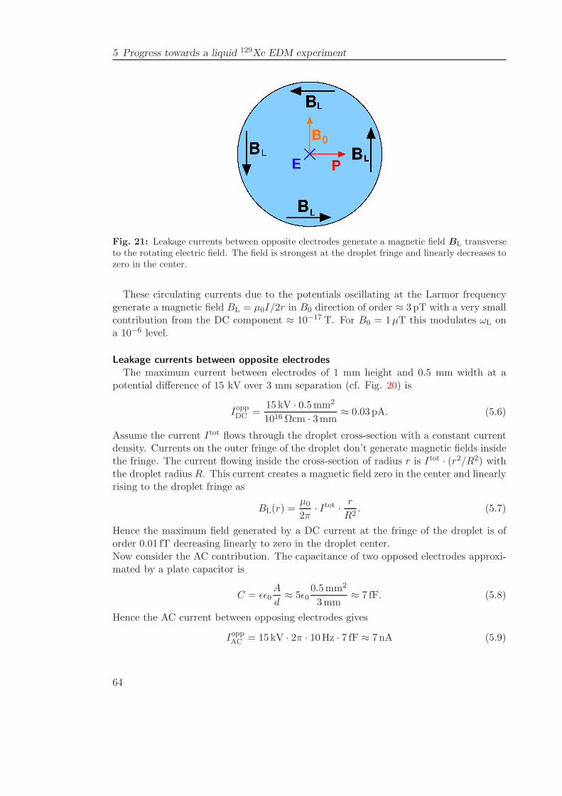
5 Progress towards a liquid 129Xe EDM experiment
Fig. 21: Leakage currents between opposite electrodes generate a magnetic field BL transverseto the rotating electric field. The field is strongest at the droplet fringe and linearly decreases tozero in the center.
These circulating currents due to the potentials oscillating at the Larmor frequencygenerate a magnetic field BL = µ0I/2r in B0 direction of order ≈ 3 pT with a very smallcontribution from the DC component ≈ 10−17 T. For B0 = 1µT this modulates ωL ona 10−6 level.
Leakage currents between opposite electrodesThe maximum current between electrodes of 1 mm height and 0.5 mm width at a
potential difference of 15 kV over 3 mm separation (cf. Fig. 20) is
IoppDC =15kV · 0.5mm2
1016 Ωcm · 3mm≈ 0.03 pA. (5.6)
Assume the current Itot flows through the droplet cross-section with a constant currentdensity. Currents on the outer fringe of the droplet don’t generate magnetic fields insidethe fringe. The current flowing inside the cross-section of radius r is Itot · (r2/R2) withthe droplet radius R. This current creates a magnetic field zero in the center and linearlyrising to the droplet fringe as
BL(r) =µ02π
· Itot · r
R2. (5.7)
Hence the maximum field generated by a DC current at the fringe of the droplet is oforder 0.01 fT decreasing linearly to zero in the droplet center.Now consider the AC contribution. The capacitance of two opposed electrodes approxi-mated by a plate capacitor is
C = ǫǫ0A
d≈ 5ǫ0
0.5mm2
3mm≈ 7 fF. (5.8)
Hence the AC current between opposing electrodes gives
IoppAC = 15kV · 2π · 10Hz · 7 fF ≈ 7 nA (5.9)
64
5.1 A novel approach to measure the EDM of 129Xe
and generates a magnetic field (Eqn. (5.7)) of order BL ≈ 3 pT at the droplet fringe,decreasing linearly to zero at the center. The gradients ∂Bx,y/∂z and ∂Bz/∂x, y in-troduced by the radial fields are of order 10 nT/m and are not limiting the anticipatedobservation time of 1000 s.
What are the consequences of the leakage currents between opposite electrodes?Components of BL that are parallel to P have no effect (BL×P = 0). But, they accountfor a false EDM if the angle between E and P deviates from π/2, similar to the case ofmotional fields in a misaligned E. Note that the effect is of opposite sign at the top andbottom of a droplet (cf. Fig. 21).Assume a misalignment of δϕ ≈ 0.02 (≈ 1). Then the opposed rotations of spins attop and bottom that locally mimic an EDM effect occur at rates 1.5 × 10⁻¹¹ s−1 and4 × 10−6 s−1 for DC and effective AC leakage currents, respectively. Particularly thelatter effect is of concern as it is much faster than the accumulation rate of θd.The atoms take about eight seconds to diffuse from one side of the droplet to the op-posing side. Many will spend a significant amount of time in the top or bottom halfsphere where this false EDM effect can accumulate at the above rates. A pickup coilplaced 1.5 mm below the droplet will mostly see the bottom half sphere (only ≈ 20%of the top half-sphere contribute to the signal) so only weak cancellation is expected.In a long measurement run of thousand seconds some averaging is expected since thenthe atoms will cross the droplet volume about 100 times. In that case the false EDMphase angle due to the leakage current can only accumulate for about 5 s (compared toθd accumlating for 1000 s). The false EDM signal is suppressed by about two ordersof magnitude, but for the above misalignment of δϕ ≈ 1 this systematic limits thesensitivity to ≈ 3× 10⁻²⁸ ecm.However, this dominant systematic effect can be tested with the reference experiment,where it is maximal (E||P ⊥ BL). If well understood it can probably be accounted forin the analysis. Also deliberate misalignment of E will help to understand and quantifyit. With diffusive suppression and a phase angle δϕ accurate to 0.01 the false EDMphase limits a measurement to d ≈ 10−30 ecm.Under these assumptions the false EDM phase due to the DC current with a rate of10−11 s−1 limits the EDM sensitivity to d ≈ 10−35 ecm.The components perpendicular to P change the holding field strength and therefore theprecession frequency directly. DC and AC currents cause a B0(1µT) field modulationon the 10−11 and 10−5 level, respectively. If the rotation frequency of the co-rotatingelectric field is static at ωL the phase angle between P and E is modulated with a max-imum amplitude of ≈ 10−5 due to the AC current. The modulation in the left and righthalf-sphere of the droplet is phase-shifted by π and the effect is to first order suppressedby cancellation in the pickup loop below the droplet.
65
5 Progress towards a liquid 129Xe EDM experiment
Crosstalk between dropletsAnother systematic effect unique for our EDM experiment is cross-talk between the
three droplets each representing a rotating dipole field. For the polarization precessingperpendicular to B0 a neighbouring droplet sees a magnetic field of order 10−11 T oscil-lating with a frequency of 2ωL, if the droplets are along a line perpendicular to B0. Thisresults in an oscillating angle θ with amplitude depending on the tip angle. However, ifB0 points along the connecting line of the droplets the cross-talk is zero, since dipolarfields generated by one droplet are parallel to the polarization vector of the neighbouringdroplet. These effects can be well studied, but suggest an alignment of the holding fieldalong the droplets to minimize the oscillation amplitude in θ. Details on these effectshave been studied in [148].Interesting effects arise, when B0 is parallel to the connecting line of the droplets, butinhomogeneous. The presence of the gradient leads to slightly different precession fre-quencies and polarization vectors are no longer aligned. In that case the polarizationvectors of the droplets start precession around the dipolar field of the neighbour droplet,which results in oscillations phase-shifted by π in both θ and φ. The amplitude of theseoscillations depend on the strength of the gradient and distance of the droplets, whilethe frequency is determined by the generated dipolar fields, e.g. the magnetization.However, droplet distance also affects the magnetic field difference due to the gradient.The described small precession around each other might offer another novel method tolook for an EDM. Instead of a gradient, the precession frequencies of both droplets couldbe misaligned by a coupling of an EDM to applied opposite electric fields parallel to theB0 direction. This competes with the same effect due to magnetic field gradients. How-ever, when using small tip angles the effect from the magnetic gradients is suppressed.Moreover, the amplitude of the induced precession grows with droplet distance. Detailson the simulated results of these effects are found in [148].
Summary of systematicsTab. 5.1 shows a summary of the discussed systematic effects. Note that some of
the estimates are rather conservative, e.g. the resistivity is taken at room temperatureand is expected to be about two orders of magnitude higher at the melting point of xenon.
The most severe systematic is a result from the AC currents due to the rotating (oroscillating) electric field. The only strategy for this false EDM phase is an extremelyaccurate alignment of the π/2 phase between E and P . For the fundamental sensitivitylevel of 10−30 ecm this needs to be accomplished at a level < 0.01. The reference dropletwhere this effect is maximal and studies with various deliberate misalignments can beused to account for this effect in the analysis.Several effects cause a modulation or variation of the B0 field. In general this is notcausing significant effects on an EDM signal, but frequency shifts and modulations of0.1mHz to 0.1 nHz. Predominantly this induces misalignment of the co-rotating electricfield vector if the phase is not adjusted.
66
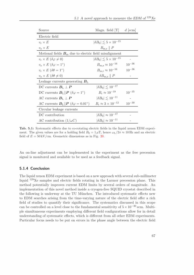
5.1 A novel approach to measure the EDM of 129Xe
Source Magn. field [T] d [ecm]
Electric field
vr × E |δB0| . 5× 10⁻¹⁵
vz × E Bm,r ‖ PMotional fields Bm due to electric field misalignment
vr × E (δϕ 6= 0) |δB0| . 5× 10⁻¹⁵ -
vz × E (δϕ = 1) Bm,z ≈ 10−16 10−36
vr × E (δθ = 1) Bm,r ≈ 10−16 10−36
vz × E (δθ 6= 0) δBm,z ‖ P -
Leakage currents generating BL
DC currents BL ⊥ P |δB0| . 10−17
DC currents BL||P (δϕ = 1) Br ≈ 10−19 10−35
AC currents BL ⊥ P |δB0| . 10−11 -
AC currents BL||P (δϕ = 0.01) Br ≈ 3× 10⁻¹² 10−30
Circular leakage currents
DC contribution |δB0| ≈ 10−17 -
AC contribution (1/ωC) |δB0| ≈ 10−11 -
Tab. 5.1: Systematic effects due to co-rotating electric fields in the liquid xenon EDM experi-ment. The given values are for a holding field B0 = 1µT, hence ωL/2π ≈ 10Hz and an electricfield of E = 50 kV/cm. Geometric dimensions as in Fig. 20.
An on-line adjustment can be implemented in the experiment as the free precessionsignal is monitored and available to be used as a feedback signal.
5.1.4 Conclusion
The liquid xenon EDM experiment is based on a new approach with several sub-millimeterliquid 129Xe samples and electric fields rotating in the Larmor precession plane. Thismethod potentially improves current EDM limits by several orders of magnitude. Animplementation of this novel method inside a cryogen-free SQUID cryostat described inthe following is underway at the TU Munchen. The introduced systematic effects newto EDM searches arising from the time-varying nature of the electric field offer a richfield of studies to quantify their significance. The systematics discussed in this scopecan be controlled on a level close to the fundamental sensitivity of 5×10⁻³⁰ ecm. Multi-ple simultaneous experiments employing different field configurations allow for in detailunderstanding of systematic effects, which is different from all other EDM experiments.Particular focus needs to be put on errors in the phase angle between the electric field
67
5 Progress towards a liquid 129Xe EDM experiment
and the precessing polarization vector. The small liquid samples offer straightforwardscaling to many simultaneous experiments.Still, by implementing electrodes above and below the liquid 129Xe droplets the setupallows for a “conventional” EDM experiment with E ‖ B0 giving similar statistic sensi-tivity, but different systematic effects.
68
5.2 A cryogen-free SQUID cryostat with variable sample temperature
5.2 A cryogen-free SQUID cryostat with variable sampletemperature
Abstract Operation of LTc SQUIDs with external pickup coils as highly sensitive cur-rent sensors is demonstrated in a cryogen-free environment allowing for unattended long-term operation. Multiple external superconducting pickup coils of two millimeter diam-eter detect local magnetic flux changes with small spacial resolution. The bottom end ofa glass tube is mounted close to the pickup coils and is used to fill gaseous samples thatcan be studied in a temperature range between 90 K to 165 K at a noise floor density of< 144 fT/
√Hz above 50 Hz. Mixing of a controlled flow of helium gas at the coldhead
allows for sample temperature control.
5.2.1 Introduction
For the detection and investigation of magnetic sample structure superconducting quan-tum interference devices (SQUIDs) are of great interest, since they provide extremelyhigh sensitivity to relative changes of magnetic flux well below 10−15 T. With the avail-ability of superconductors with critical temperatures Tc > 77K SQUIDs can be operatedeven in liquid nitrogen. Nevertheless, high-Tc (HTc) SQUIDs have disadvantages overdevices made of low critical temperature superconductors, e.g. LTc SQUIDs. HTcSQUIDS show significantly higher white and 1/f noise and ,due to their short coherencelength, can only be fabricated in one-dimensional structures. To fully use the superiornoise performance of LTc SQUIDs they need to be operated at or below half of thetransition temperature (cf. [135]). Hence, for widely used niobium the operating tem-perature should be below 4.6 K. A bath of liquid helium (LHe) at 4.2 K provides perfectconditions for SQUID sensors of the LTc type. But, this experimental approach bringsalong challenges in dewar construction and operational drawbacks for highly sensitivelong-term measurements in low magnetic fields. In particular, measurements of spin-precession require not only non-metallic (low magnetic noise) but also non-magnetic(small magnetic gradient) environments. These types of measurements with SQUIDsemerged in liquid helium require magnetically shielded rooms of significant size.Measurements at a short distance (< 1mm) of the superconducting pickup coils to sam-ples at much higher temperature is experimentally very difficult. Hence, a liquid heliumbath for the SQUID sensor is often combined with a thermal connection to an externalpickup coil.. In the “SQUID microscopes” usually a high spatial resolution is aspired formagnetic scanning of samples. As an example Baudenbacher et al. [149] demonstrateda “SQUID microscope” with a pickup loop distance on the order of 100 µm to a room-temperature sample. In their dewar with 24 h hold time they also introduced a liquidnitrogen shield which complicates operation and refilling even further. The noise levelachieved is on the order of 300 fT/
√Hz.
In this paper we demonstrate operation of LTc SQUIDs cooled by a closed-cycle coolingmachine (Gifford-MacMahon type) without the need of cryogens in the SQUID setup,while a sample of variable temperature can be studied. The setup enables unattendedlong-term operation of SQUIDs kept in vacuum, while a magnetic flux noise density of
69
5 Progress towards a liquid 129Xe EDM experiment
49 fT/√Hz and 165 fT/
√Hz is demonstrated for gradiometer and magnetometer pickup
coils, respectively. These levels of the noise floor were measured in the frequency rangeabove 50 Hz.A drawback of using a coldhead and conductive cooling is certainly the vibrations causedby the moving parts and low frequency noise due to inevitable use of metallic parts inthe setup. Several noise peaks are detected in the setup that are mostly related to theseeffects. However, this strongly depends on the purpose of the system and low frequencynoise might be less of a concern.In the setup highly sensitive measurements of magnetic flux changes can be taken outin a homogeneous small residual magnetic field without the need of large helium dewarsor even magnetically shielded rooms. The non-magnetic vacuum and cryogenic part ofthe SQUID system is fed through a hole of less than 80 mm diameter in the magneticshielding.The presented SQUID cryostat is intended to be used for fundamental measurementsusing ultra low-field nuclear magnetic resonance (NMR) in magnetic fields of the order of0.1− 10 µT. Of special interest is a measurement of the electric dipole moment (EDM)of the isotope 129Xe. A non-zero EDM is a strong manifestation of physics beyondthe standard model violating fundamental symmetries [31, 33]. Furthermore, studies ofsolid and liquid polarized xenon in very low fields as well as a search of (more exotic)spin-matter couplings are anticipated.
5.2.2 Apparatus
OverviewThe apparatus is mounted in a vertically hanging position with the coldhead on top.
Two mechanically independent holding structures made of massive aluminum profilescarry both the vacuum vessel housing the coldhead in a height of 2.5 m and fix thenon-magnetic vacuum system. Rectangular coils with 2 m side length are mounted foreach spacial axis to compensate the earth’s magnetic field and external gradient fields,but are not yet used. The whole setup is enclosed by a 3.5 m x 3.5 m x 3.5 m styrofoamcube for thermal stabilization of the magnetic shield and damping of external vibrations.Most electrical devices and the compressor unit for the coldhead are placed at a distanceof several meters outside the styrofoam housing.
Electrical radio-frequency shielding is provided by the grounded vacuum system. Fourlayers of µ-metal (a high magnetic permeability nickel-iron alloy) enclose the vacuumsystem (Fig. 17) for magnetic shielding. The layers are made of top caps fixed on thetop vacuum lid and cylinders with closed bottom ends which have a thickness of 1mmbut the second layer is of 2mm thickness. The magnetically shielded volume for ultralow-field experiments is about 1 m below the coldhead and of dimensions of 560 mmheight and 230 mm diameter. The µ-metal shield only has several small holes on thecylinder surface (5 mm and 8 mm diameter) and the center of the cylinder bottom (20mm diameter). A 80 mm hole in the top caps is needed to feed-through the vacuumvessel including wiring, thermal shield and connection to the 4 K stage of the coldhead.
70
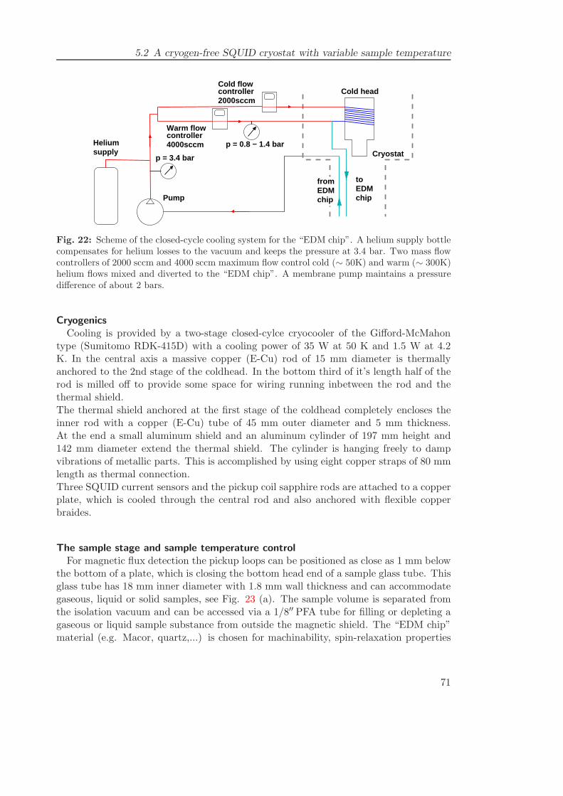
5.2 A cryogen-free SQUID cryostat with variable sample temperature
EDM
p = 3.4 bar
p = 0.8 − 1.4 bar
chipEDM
chip
supply
to from
Helium
Pump
Cold head
Cryostat
2000sccm controllerCold flow
Warm flowcontroller4000sccm
Fig. 22: Scheme of the closed-cycle cooling system for the “EDM chip”. A helium supply bottlecompensates for helium losses to the vacuum and keeps the pressure at 3.4 bar. Two mass flowcontrollers of 2000 sccm and 4000 sccm maximum flow control cold (∼ 50K) and warm (∼ 300K)helium flows mixed and diverted to the “EDM chip”. A membrane pump maintains a pressuredifference of about 2 bars.
CryogenicsCooling is provided by a two-stage closed-cylce cryocooler of the Gifford-McMahon
type (Sumitomo RDK-415D) with a cooling power of 35 W at 50 K and 1.5 W at 4.2K. In the central axis a massive copper (E-Cu) rod of 15 mm diameter is thermallyanchored to the 2nd stage of the coldhead. In the bottom third of it’s length half of therod is milled off to provide some space for wiring running inbetween the rod and thethermal shield.The thermal shield anchored at the first stage of the coldhead completely encloses theinner rod with a copper (E-Cu) tube of 45 mm outer diameter and 5 mm thickness.At the end a small aluminum shield and an aluminum cylinder of 197 mm height and142 mm diameter extend the thermal shield. The cylinder is hanging freely to dampvibrations of metallic parts. This is accomplished by using eight copper straps of 80 mmlength as thermal connection.Three SQUID current sensors and the pickup coil sapphire rods are attached to a copperplate, which is cooled through the central rod and also anchored with flexible copperbraides.
The sample stage and sample temperature controlFor magnetic flux detection the pickup loops can be positioned as close as 1 mm below
the bottom of a plate, which is closing the bottom head end of a sample glass tube. Thisglass tube has 18 mm inner diameter with 1.8 mm wall thickness and can accommodategaseous, liquid or solid samples, see Fig. 23 (a). The sample volume is separated fromthe isolation vacuum and can be accessed via a 1/8′′ PFA tube for filling or depleting agaseous or liquid sample substance from outside the magnetic shield. The “EDM chip”material (e.g. Macor, quartz,...) is chosen for machinability, spin-relaxation properties
71
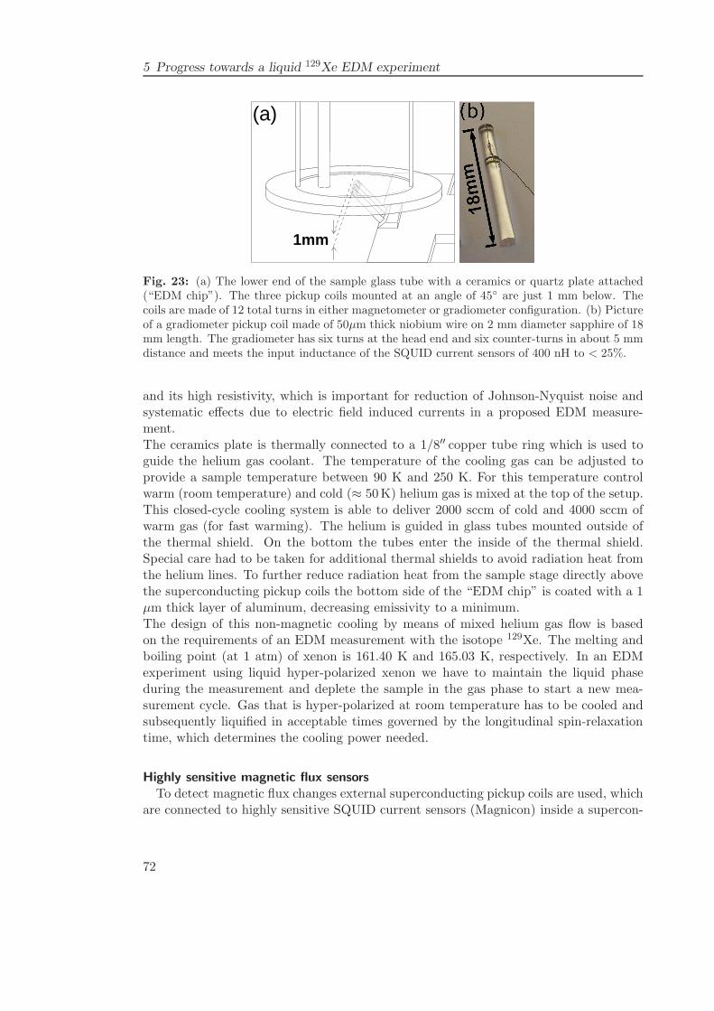
5 Progress towards a liquid 129Xe EDM experiment
1mm
(a)
Fig. 23: (a) The lower end of the sample glass tube with a ceramics or quartz plate attached(“EDM chip”). The three pickup coils mounted at an angle of 45 are just 1 mm below. Thecoils are made of 12 total turns in either magnetometer or gradiometer configuration. (b) Pictureof a gradiometer pickup coil made of 50µm thick niobium wire on 2 mm diameter sapphire of 18mm length. The gradiometer has six turns at the head end and six counter-turns in about 5 mmdistance and meets the input inductance of the SQUID current sensors of 400 nH to < 25%.
and its high resistivity, which is important for reduction of Johnson-Nyquist noise andsystematic effects due to electric field induced currents in a proposed EDM measure-ment.The ceramics plate is thermally connected to a 1/8′′ copper tube ring which is used toguide the helium gas coolant. The temperature of the cooling gas can be adjusted toprovide a sample temperature between 90 K and 250 K. For this temperature controlwarm (room temperature) and cold (≈ 50K) helium gas is mixed at the top of the setup.This closed-cycle cooling system is able to deliver 2000 sccm of cold and 4000 sccm ofwarm gas (for fast warming). The helium is guided in glass tubes mounted outside ofthe thermal shield. On the bottom the tubes enter the inside of the thermal shield.Special care had to be taken for additional thermal shields to avoid radiation heat fromthe helium lines. To further reduce radiation heat from the sample stage directly abovethe superconducting pickup coils the bottom side of the “EDM chip” is coated with a 1µm thick layer of aluminum, decreasing emissivity to a minimum.The design of this non-magnetic cooling by means of mixed helium gas flow is basedon the requirements of an EDM measurement with the isotope 129Xe. The melting andboiling point (at 1 atm) of xenon is 161.40 K and 165.03 K, respectively. In an EDMexperiment using liquid hyper-polarized xenon we have to maintain the liquid phaseduring the measurement and deplete the sample in the gas phase to start a new mea-surement cycle. Gas that is hyper-polarized at room temperature has to be cooled andsubsequently liquified in acceptable times governed by the longitudinal spin-relaxationtime, which determines the cooling power needed.
Highly sensitive magnetic flux sensorsTo detect magnetic flux changes external superconducting pickup coils are used, which
are connected to highly sensitive SQUID current sensors (Magnicon) inside a supercon-
72
5.2 A cryogen-free SQUID cryostat with variable sample temperature
ducting shield. Operated in a flux-locked loop (FFL) mode these sensors exhibit anintrinsic noise level of < 2 fT/
√Hz and a 1/f noise edge at 3 Hz. The sensors have
an input inductance of 400 nH and an input coupling of 0.5µA/Φ0, with Φ0 being themagnetic flux quantum. The sensitivity of the FLL feedback circuit is 42 − 44µA/Φ0
slightly varying for different channels.Twelve turns of niobium wire (Goodfellow, 7µm polyimide insulation, 50µm diameter)on sapphire (2.0 mm diameter, 18 mm length) are prepared either as magnetometer orgradiometer (baseline 3-5 mm) pickup coils (see Fig. 23). The geometry of the coils israther determined by the requirements for an EDM measurement than limited experi-mentally. In the current setup three coils mounted in line with a distance of 5 mm areconnected to SQUID sensors. The connecting wire pairs of the coils are twisted to avoidpickup of stray fields, while they are mostly routed inside the SQUID’s superconductingniobium capsule.The input impedance of 400 nH can be matched very well with twelve windings. Induc-tances measured with a LCR meter (Standford Research SR720) are between 300 nHand 370 nH. The signal wires from the room temperature SQUID electronics (Magnicon)to the current sensors are attached to the thermal shield outside the magnetic shield andthen routed down inside the thermal shield. Finally the cable manifold is attached tothe end of the central copper rod to provide contact to the 4 K stage. The SQUIDsensors as well as three pickup coils are thermally anchored to the cooled copper platevia sixteen little copper straps (2 mm diameter) of 40 mm length. The SQUID sensorsare mounted roughly in the center axis, whereas the sapphire rods with the pickup coilshave a position 40 mm off-axis and tilted at an angle of 45. Due to the high masstemperature variations of the SQUID sensors are within 20 mK, cf. Fig. 24 (a). Inprincipal, by implementing additional SQUID sensors the number of channels can easilybe increased.In FLL mode the externally induced current fed into the SQUID generates a magneticflux in an internal loop, which is canceled by a field generated by a current in a feedbackloop. This current controlled by the FLL electronics is measured as a voltage drop over aresistor of variable size (1 kΩ to 100 kΩ) in the feedback loop. The voltage data from thethree SQUID channels is acquired with a fast 24-bit ADC card (National Instruments,NI-4662).Calibration of the SQUID signal to a known magnetic field yields a conversion factorfor the flux-to-voltage transformation of 23 nT/V and 46 nT/V for magnetometers andgradiometers, respectively (Fig. 28). This agrees very well with the specified input andmutual inductances.
Magnetic flux noise and mechanical vibrationsA main source of mechanical vibration is the piston in the coldhead, which moves
at about 1 Hz. To reduce mechanical (and hence magnetic flux) vibrations to a mini-mum thermal connections are made of flexible copper straps. Installed parts inside themagnetic shield are made of non-magnetic materials and were screened at PTB Berlin
73
5 Progress towards a liquid 129Xe EDM experiment
to avoid magnetic contamination and gradients in the setup. However, in the measure-ments presented here, a magnetic silicon diode temperature sensor was mounted on thecoldplate, which probably introduces strong magnetic noise due to vibrations.
Johnson-Nyquist noiseAnother source of magnetic flux noise are current fluctuations in metallic parts due
to thermal movement of electrons (Johnson-Nyquist noise). The current noise density ofa resistor R is i =
√4πkBT/R, with the temperature T and Boltzmann’s constant kB.
At temperatures of 4 K and milliohm resistance Johnson-Nyquist noise accounts for amagnetic flux noise density of several fT/
√Hz in some millimeter distance. The super-
conducting pickup loops mounted on sapphire rods of 18 mm length are at a distance> 10mm to massive metallic parts at 4 K which yields Johnson-Nyquist noise of order1 fT/
√Hz. But, the the copper cooling tube and an aluminum part fixing the copper
tube are at temperatures of order 100 K and the distance to the pickup loops is of order 5mm. Measured noise levels of several tens of fT/
√Hz might arise from Johnson-Nyquist
noise of these metallic parts and can currently be limiting the achievable noise levels.
Magnetic field coilsTo perform an EDM experiment with a liquid Xenon sample we need to apply ultra-
low field NMR techniques (e.g. control over nuclear spin orientation). Therefore, onecylindrical coil and two cosine-theta coils are implemented inside the magnetic shieldto provide magnetic fields of up to 100 µT in all three spacial directions. These coilsare printed on double-sided flexible circuit boards with 1 mm wide and 70µm thickcopper conductors and non-magnetic tin (trough-)contacts. All three flexible circuitboards are attached to the outer surface of a rigid plastic tube of 350 mm length and anouter diameter of 224 mm. This tube is placed inside the innermost magnetic shieldingcylinder and pushed over the vacuum system when assembling the magnetic shields (cf.Fig. 17).The two equal cosine-theta coils have a height of 260 mm and provide perpendicularmagnetic fields transverse to the axis of the magnetic shielding cylinders (400µT/A).The use of printed flexible circuit boards assures a geometrically very accurate currentdistribution giving rise to good magnetic field homogeneity. With a current-cancelinglayout simulations of the generated magnetic fields show a relative homogeneity on a <10−4 level over a 1 cm3 volume. This can be improved by introducing printed correctioncoils of nearly arbitrary shape placed on the field coils.A cylindrical coil for generation of magnetic fields (125µT/A) in the vertical directionconsists of 34 windings with 20 mm separation exactly perpendicular to the coil axis.This avoids small tilt angles of the magnetic field when using wire-wound coils. Theconnection to the next-neighbour winding is done with two steps to cancel all verticalcomponents of the magnetic field generated.This magnetic field configuration allows for holding fields in all three spacial directionsand rotating perpendicular magnetic fields, which are all very well aligned to each otherdue to the use of flexible circuits.
74
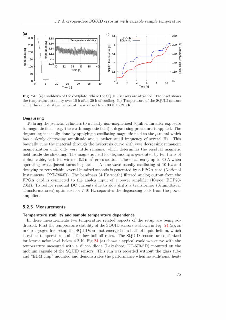
5.2 A cryogen-free SQUID cryostat with variable sample temperature
0
50
100
150
200
250
300
0 5 10 15 20 25 30
Tem
pera
ture
[K]
Time [h]
(a)
3.08
3.1
3.12
3.14
3.16
3.18
30 32 34 36 38 40
Tem
pera
ture
[K]
Time [h]
(a)
Temperature stability
3
3.5
4
4.5
5
5.5
0 2 4 6 8 10 80
110
140
170
200
230
SQ
UID
tem
pera
ture
[K]
ED
M c
hip
tem
pera
ture
[K]
Time [h]
(b)SQUID
EDM chip
Fig. 24: (a) Cooldown of the coldplate, where the SQUID sensors are attached. The inset showsthe temperature stability over 10 h after 30 h of cooling. (b) Temperature of the SQUID sensorswhile the sample stage temperature is varied from 90 K to 210 K.
DegaussingTo bring the µ-metal cylinders to a nearly non-magnetized equilibrium after exposure
to magnetic fields, e.g. the earth magnetic field) a degaussing procedure is applied. Thedegaussing is usually done by applying a oscillating magnetic field to the µ-metal whichhas a slowly decreasing amplitude and a rather small frequency of several Hz. Thisbasically runs the material through the hysteresis curve with ever decreasing remanentmagnetization until only very little remains, which determines the residual magneticfield inside the shielding. The magnetic field for degaussing is generated by ten turns ofribbon cable, each ten wires of 0.5mm2 cross section. These can carry up to 30 A whenoperating two adjacent turns in parallel. A sine wave usually oscillating at 10 Hz anddecaying to zero within several hundred seconds is generated by a FPGA card (NationalInstruments, PXI-7853R). The bandpass (4 Hz width) filtered analog output from theFPGA card is connected to the analog input of a power amplifier (Kepco, BOP20-20M). To reduce residual DC currents due to slow drifts a transformer (SchmidbauerTransformatoren) optimized for 7-10 Hz separates the degaussing coils from the poweramplifier.
5.2.3 Measurements
Temperature stability and sample temperature dependenceIn these measurements two temperature related aspects of the setup are being ad-
dressed. First the temperature stability of the SQUID sensors is shown in Fig. 24 (a), asin our cryogen-free setup the SQUIDs are not emerged in a bath of liquid helium, whichis rather temperature stable for low boil-off rates. The SQUID sensors are optimizedfor lowest noise level below 4.2 K. Fig 24 (a) shows a typical cooldown curve with thetemperature measured with a silicon diode (Lakeshore, DT-670-SD) mounted on theniobium capsule of the SQUID sensors. This run was recorded without the glass tubeand “EDM chip” mounted and demonstrates the performance when no additional heat-
75
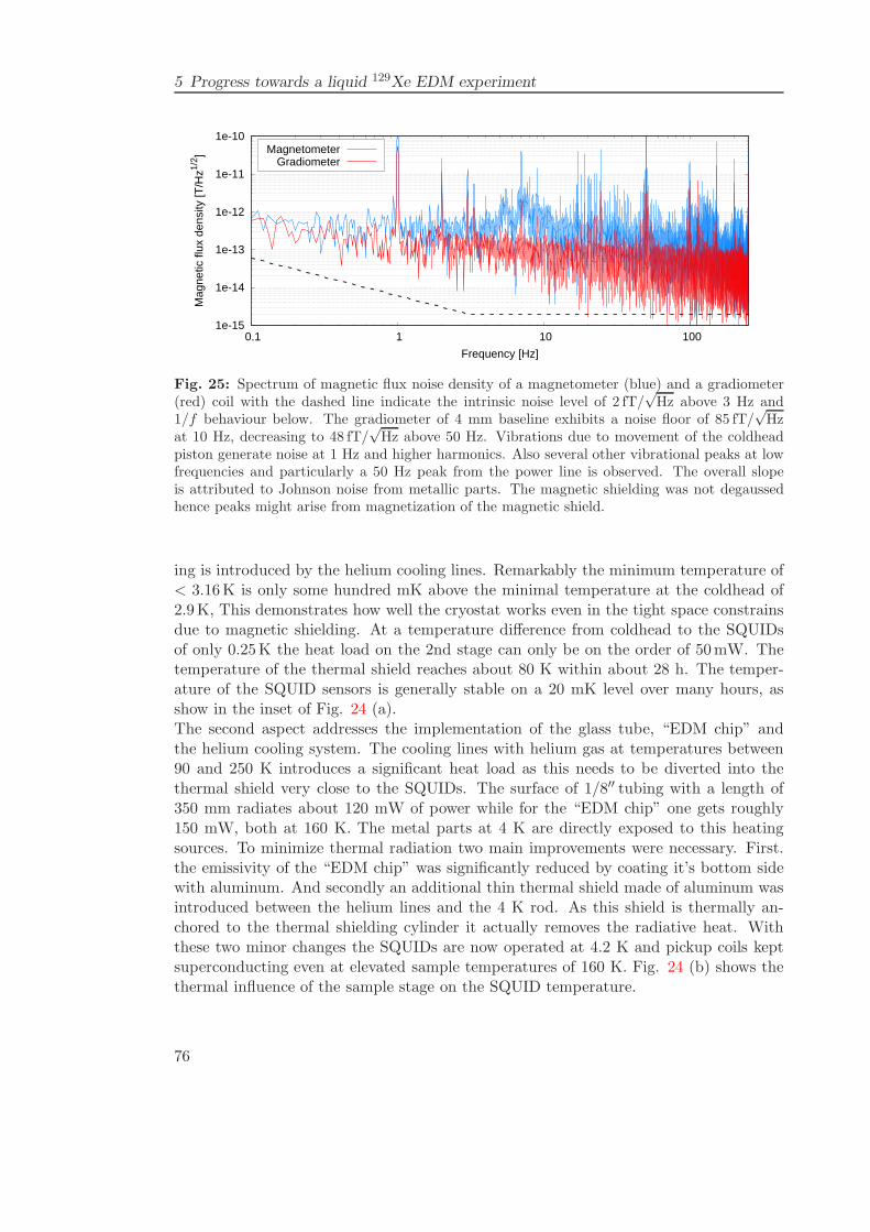
5 Progress towards a liquid 129Xe EDM experiment
1e-15
1e-14
1e-13
1e-12
1e-11
1e-10
0.1 1 10 100
Mag
netic
flux
den
sity
[T/H
z1/2 ]
Frequency [Hz]
MagnetometerGradiometer
Fig. 25: Spectrum of magnetic flux noise density of a magnetometer (blue) and a gradiometer(red) coil with the dashed line indicate the intrinsic noise level of 2 fT/
√Hz above 3 Hz and
1/f behaviour below. The gradiometer of 4 mm baseline exhibits a noise floor of 85 fT/√Hz
at 10 Hz, decreasing to 48 fT/√Hz above 50 Hz. Vibrations due to movement of the coldhead
piston generate noise at 1 Hz and higher harmonics. Also several other vibrational peaks at lowfrequencies and particularly a 50 Hz peak from the power line is observed. The overall slopeis attributed to Johnson noise from metallic parts. The magnetic shielding was not degaussedhence peaks might arise from magnetization of the magnetic shield.
ing is introduced by the helium cooling lines. Remarkably the minimum temperature of< 3.16K is only some hundred mK above the minimal temperature at the coldhead of2.9K, This demonstrates how well the cryostat works even in the tight space constrainsdue to magnetic shielding. At a temperature difference from coldhead to the SQUIDsof only 0.25K the heat load on the 2nd stage can only be on the order of 50mW. Thetemperature of the thermal shield reaches about 80 K within about 28 h. The temper-ature of the SQUID sensors is generally stable on a 20 mK level over many hours, asshow in the inset of Fig. 24 (a).The second aspect addresses the implementation of the glass tube, “EDM chip” andthe helium cooling system. The cooling lines with helium gas at temperatures between90 and 250 K introduces a significant heat load as this needs to be diverted into thethermal shield very close to the SQUIDs. The surface of 1/8′′ tubing with a length of350 mm radiates about 120 mW of power while for the “EDM chip” one gets roughly150 mW, both at 160 K. The metal parts at 4 K are directly exposed to this heatingsources. To minimize thermal radiation two main improvements were necessary. First.the emissivity of the “EDM chip” was significantly reduced by coating it’s bottom sidewith aluminum. And secondly an additional thin thermal shield made of aluminum wasintroduced between the helium lines and the 4 K rod. As this shield is thermally an-chored to the thermal shielding cylinder it actually removes the radiative heat. Withthese two minor changes the SQUIDs are now operated at 4.2 K and pickup coils keptsuperconducting even at elevated sample temperatures of 160 K. Fig. 24 (b) shows thethermal influence of the sample stage on the SQUID temperature.
76
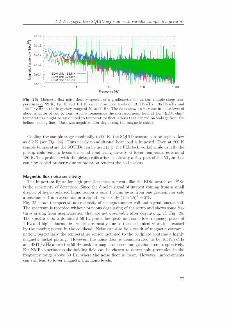
5.2 A cryogen-free SQUID cryostat with variable sample temperature
1e-15
1e-14
1e-13
1e-12
1e-11
1e-10
0.1 1 10 100 1000
Mag
netic
flux
den
sity
[T/H
z1/2 ]
Frequency [Hz]
EDM chip 91.8 KEDM chip 126.0 KEDM chip 160.7 K
Fig. 26: Magnetic flux noise density spectra of a gradiometer for various sample stage tem-peratures of 92 K, 126 K and 161 K yield noise floor levels of 131 fT/
√Hz, 135 fT/
√Hz and
144 fT/√Hz in the frequency range of 50 to 90 Hz. The data show an increase in noise level of
about a factor of two to four. At low frequencies the increased noise level at low “EDM chip”temperatures might be attributed to temperature fluctuations that depend on leakage from thehelium cooling lines. Data was acquired after degaussing the magnetic shields.
Cooling the sample stage maximally to 90 K, the SQUID sensors can be kept as lowas 3.2 K (see Fig. 24). Thus nearly no additional heat load is imposed. Even at 200 Ksample temperature the SQUIDs can be used (e.g. the FLL lock works) while usually thepickup coils tend to become normal conducting already at lower temperatures around180 K. The problem with the pickup coils arises as already a tiny part of the 50 µm thatcan’t by cooled properly due to radiation renders the coil useless.
Magnetic flux noise sensitivityThe important figure for high precision measurements like the EDM search on 129Xe
is the sensitivity of detection. Since the dipolar signal of interest coming from a smalldroplet of hyper-polaized liquid xenon is only 1.5 mm away from one gradiometer sidea baseline of 4 mm accounts for a signal-loss of only (1.5/5.5)3 = 2%.Fig. 25 shows the spectral noise density of a magnetometer coil and a gradiometer coil.The spectrum is recorded without previous degaussing of the setup and shows some fea-tures arising from magnetization that are not observable after degaussing, cf. Fig. 26.The spectra show a dominant 50 Hz power line peak and some low-frequency peaks of1 Hz and higher harmonics, which are mostly due to the mechanical vibrations causedby the moving piston in the coldhead. Noise can also be a result of magnetic contami-nation, particularly the temperature sensor mounted to the coldplate contains a highlymagnetic nickel plating. However, the noise floor is demonstrated to be 165 fT/
√Hz
and 48 fT/√Hz above the 50 Hz peak for magnetometers and gradiometers, respectively.
For NMR experiments the holding field can be chosen to detect spin precession in thefrequency range above 50 Hz, where the noise floor is lower. However, improvementscan still lead to lower magnetic flux noise levels.
77
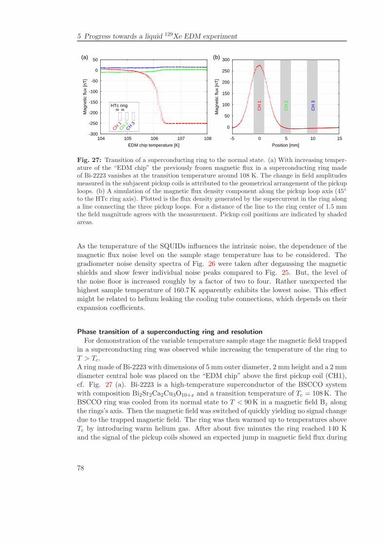
5 Progress towards a liquid 129Xe EDM experiment
-300
-250
-200
-150
-100
-50
0
50
104 105 106 107 108
Mag
netic
flux
[nT
]
EDM chip temperature [K]
(a)
HTc ring
CH 1CH 2
CH 3 0
50
100
150
200
250
300
-5 0 5 10 15
Mag
netic
flux
[nT
]
Position [mm]
(b)
CH
1
CH
2
CH
3
Fig. 27: Transition of a superconducting ring to the normal state. (a) With increasing temper-ature of the “EDM chip” the previously frozen magnetic flux in a superconducting ring madeof Bi-2223 vanishes at the transition temperature around 108 K. The change in field amplitudesmeasured in the subjacent pickup coils is attributed to the geometrical arrangement of the pickuploops. (b) A simulation of the magnetic flux density component along the pickup loop axis (45
to the HTc ring axis). Plotted is the flux density generated by the supercurrent in the ring alonga line connecting the three pickup loops. For a distance of the line to the ring center of 1.5 mmthe field magnitude agrees with the measurement. Pickup coil positions are indicated by shadedareas.
As the temperature of the SQUIDs influences the intrinsic noise, the dependence of themagnetic flux noise level on the sample stage temperature has to be considered. Thegradiometer noise density spectra of Fig. 26 were taken after degaussing the magneticshields and show fewer individual noise peaks compared to Fig. 25. But, the level ofthe noise floor is increased roughly by a factor of two to four. Rather unexpected thehighest sample temperature of 160.7K apparently exhibits the lowest noise. This effectmight be related to helium leaking the cooling tube connections, which depends on theirexpansion coefficients.
Phase transition of a superconducting ring and resolutionFor demonstration of the variable temperature sample stage the magnetic field trapped
in a superconducting ring was observed while increasing the temperature of the ring toT > Tc.A ring made of Bi-2223 with dimensions of 5 mm outer diameter, 2 mm height and a 2 mmdiameter central hole was placed on the “EDM chip” above the first pickup coil (CH1),cf. Fig. 27 (a). Bi-2223 is a high-temperature superconductor of the BSCCO systemwith composition Bi2Sr2Ca2Cu3O10+x and a transition temperature of Tc = 108K. TheBSCCO ring was cooled from its normal state to T < 90K in a magnetic field Bz alongthe rings’s axis. Then the magnetic field was switched of quickly yielding no signal changedue to the trapped magnetic field. The ring was then warmed up to temperatures aboveTc by introducing warm helium gas. After about five minutes the ring reached 140 Kand the signal of the pickup coils showed an expected jump in magnetic field flux during
78
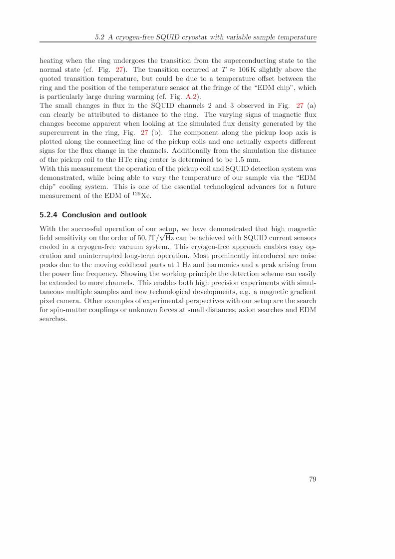
5.2 A cryogen-free SQUID cryostat with variable sample temperature
heating when the ring undergoes the transition from the superconducting state to thenormal state (cf. Fig. 27). The transition occurred at T ≈ 106K slightly above thequoted transition temperature, but could be due to a temperature offset between thering and the position of the temperature sensor at the fringe of the “EDM chip”, whichis particularly large during warming (cf. Fig. A.2).The small changes in flux in the SQUID channels 2 and 3 observed in Fig. 27 (a)can clearly be attributed to distance to the ring. The varying signs of magnetic fluxchanges become apparent when looking at the simulated flux density generated by thesupercurrent in the ring, Fig. 27 (b). The component along the pickup loop axis isplotted along the connecting line of the pickup coils and one actually expects differentsigns for the flux change in the channels. Additionally from the simulation the distanceof the pickup coil to the HTc ring center is determined to be 1.5 mm.With this measurement the operation of the pickup coil and SQUID detection system wasdemonstrated, while being able to vary the temperature of our sample via the “EDMchip” cooling system. This is one of the essential technological advances for a futuremeasurement of the EDM of 129Xe.
5.2.4 Conclusion and outlook
With the successful operation of our setup, we have demonstrated that high magneticfield sensitivity on the order of 50, fT/
√Hz can be achieved with SQUID current sensors
cooled in a cryogen-free vacuum system. This cryogen-free approach enables easy op-eration and uninterrupted long-term operation. Most prominently introduced are noisepeaks due to the moving coldhead parts at 1 Hz and harmonics and a peak arising fromthe power line frequency. Showing the working principle the detection scheme can easilybe extended to more channels. This enables both high precision experiments with simul-taneous multiple samples and new technological developments, e.g. a magnetic gradientpixel camera. Other examples of experimental perspectives with our setup are the searchfor spin-matter couplings or unknown forces at small distances, axion searches and EDMsearches.
79
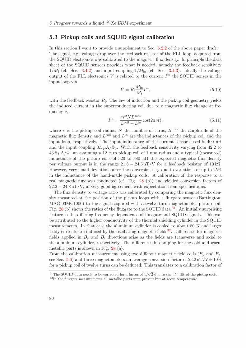
5 Progress towards a liquid 129Xe EDM experiment
5.3 Pickup coils and SQUID signal calibration
In this section I want to provide a supplement to Sec. 5.2.2 of the above paper draft.The signal, e.g. voltage drop over the feedback resistor of the FLL loop, acquired fromthe SQUID electronics was calibrated to the magnetic flux density. In principle the datasheet of the SQUID sensors provides what is needed, namely the feedback sensitivity1/Mf (cf. Sec. 3.4.2) and input coupling 1/Min (cf. Sec. 3.4.3). Ideally the voltageoutput of the FLL electronics V is related to the current I in the SQUID senses in theinput loop via
V = RfMin
MfI in, (5.10)
with the feedback resistor Rf. The law of induction and the pickup coil geometry yieldsthe induced current in the superconducting coil due to a magnetic flux change at fre-quency ν,
I in =πr2NBmax
Lcoil + Lincos(2πνt), (5.11)
where r is the pickup coil radius, N the number of turns, Bmax the amplitude of themagnetic flux density and Lcoil and Lin are the inductances of the pickup coil and theinput loop, respectively. The input inductance of the current sensors used is 400 nHand the input coupling 0.5µA/Φ0. With the feedback sensitivity varying from 42.2 to43.8µA/Φ0 an assuming a 12 turn pickup coil of 1 mm radius and a typical (measured)inductance of the pickup coils of 320 to 380 nH the expected magnetic flux densityper voltage output is in the range 21.8 − 24.5 nT/V for a feedback resistor of 10 kΩ.However, very small deviations alter the conversion e.g. due to variations of up to 25%in the inductance of the hand-made pickup coils. A calibration of the response to areal magnetic flux was conducted (cf. Fig. 28 (b)) and yielded conversion factors of22.2 − 24.8 nT/V, in very good agreement with expectation from specifications.
The flux density to voltage ratio was calibrated by comparing the magnetic flux den-sity measured at the position of the pickup loops with a fluxgate sensor (Bartington,MAG-03MC1000) to the signal acquired with a twelve-turn magnetometer pickup coil.Fig. 28 (b) shows the ratios of the fluxgate to the SQUID data.31. An initially surprisingfeature is the differing frequency dependence of fluxgate and SQUID signals. This canbe attributed to the higher conductivity of the thermal shielding cylinder in the SQUIDmeasurements. In that case the aluminum cylinder is cooled to about 80 K and largerEddy currents are induced by the oscillating magnetic fields32. Differences for magneticfields applied in By and Bz directions arise as the fields are transverse and axial tothe aluminum cylinder, respectively. The differences in damping for the cold and warmmetallic parts is shown in Fig. 28 (a).From the calibration measurement using two different magnetic field coils (By and Bz,see Sec. 5.6) and three magnetometers an average conversion factor of 23.2 nT/V± 10%for a pickup coil of twelve turns can be deduced. This translates to a calibration factor of
31The SQUID data needs to be corrected for a factor of 1/√2 due to the 45 tilt of the pickup coils.
32In the fluxgate measurements all metallic parts were present but at room temperature
80
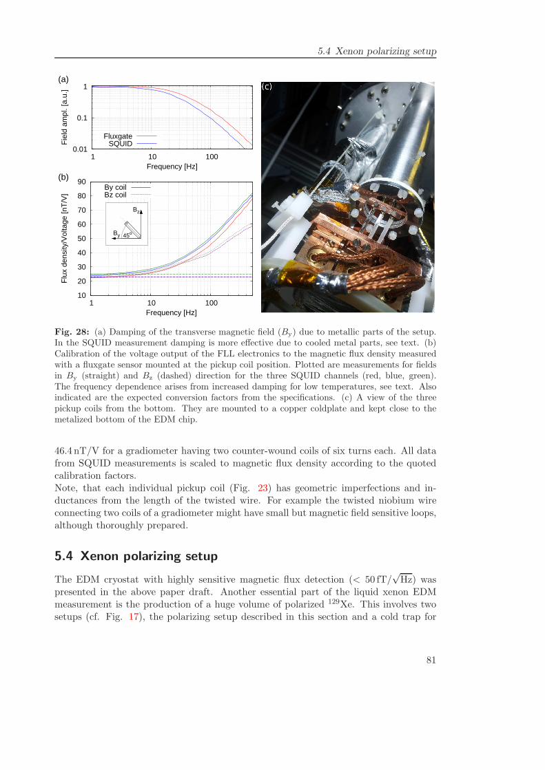
5.4 Xenon polarizing setup
0.01
0.1
1
1 10 100
Fie
ld a
mpl
. [a.
u.]
Frequency [Hz]
(a)
FluxgateSQUID
10
20
30
40
50
60
70
80
90
1 10 100
Flu
x de
nsity
/Vol
tage
[nT
/V]
Frequency [Hz]
(b)By coilBz coil
Bz
By 45o
Fig. 28: (a) Damping of the transverse magnetic field (By) due to metallic parts of the setup.In the SQUID measurement damping is more effective due to cooled metal parts, see text. (b)Calibration of the voltage output of the FLL electronics to the magnetic flux density measuredwith a fluxgate sensor mounted at the pickup coil position. Plotted are measurements for fieldsin By (straight) and Bz (dashed) direction for the three SQUID channels (red, blue, green).The frequency dependence arises from increased damping for low temperatures, see text. Alsoindicated are the expected conversion factors from the specifications. (c) A view of the threepickup coils from the bottom. They are mounted to a copper coldplate and kept close to themetalized bottom of the EDM chip.
46.4 nT/V for a gradiometer having two counter-wound coils of six turns each. All datafrom SQUID measurements is scaled to magnetic flux density according to the quotedcalibration factors.Note, that each individual pickup coil (Fig. 23) has geometric imperfections and in-ductances from the length of the twisted wire. For example the twisted niobium wireconnecting two coils of a gradiometer might have small but magnetic field sensitive loops,although thoroughly prepared.
5.4 Xenon polarizing setup
The EDM cryostat with highly sensitive magnetic flux detection (< 50 fT/√Hz) was
presented in the above paper draft. Another essential part of the liquid xenon EDMmeasurement is the production of a huge volume of polarized 129Xe. This involves twosetups (cf. Fig. 17), the polarizing setup described in this section and a cold trap for
81
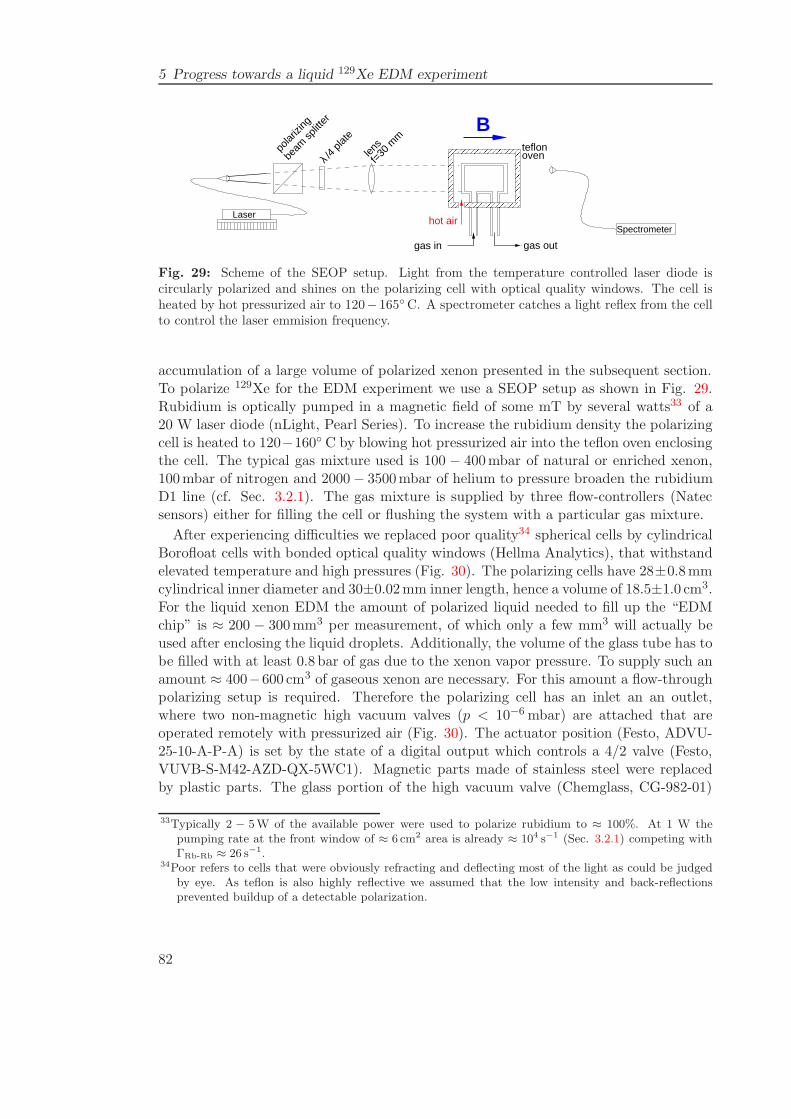
5 Progress towards a liquid 129Xe EDM experiment
Spectrometer
Laserhot air
B
gas in gas out
λ /4 p
late
beam
splitt
er
polar
izing
f=30
mm
lens
oventeflon
Fig. 29: Scheme of the SEOP setup. Light from the temperature controlled laser diode iscircularly polarized and shines on the polarizing cell with optical quality windows. The cell isheated by hot pressurized air to 120− 165C. A spectrometer catches a light reflex from the cellto control the laser emmision frequency.
accumulation of a large volume of polarized xenon presented in the subsequent section.To polarize 129Xe for the EDM experiment we use a SEOP setup as shown in Fig. 29.Rubidium is optically pumped in a magnetic field of some mT by several watts33 of a20 W laser diode (nLight, Pearl Series). To increase the rubidium density the polarizingcell is heated to 120−160 C by blowing hot pressurized air into the teflon oven enclosingthe cell. The typical gas mixture used is 100 − 400mbar of natural or enriched xenon,100mbar of nitrogen and 2000− 3500mbar of helium to pressure broaden the rubidiumD1 line (cf. Sec. 3.2.1). The gas mixture is supplied by three flow-controllers (Natecsensors) either for filling the cell or flushing the system with a particular gas mixture.
After experiencing difficulties we replaced poor quality34 spherical cells by cylindricalBorofloat cells with bonded optical quality windows (Hellma Analytics), that withstandelevated temperature and high pressures (Fig. 30). The polarizing cells have 28±0.8mmcylindrical inner diameter and 30±0.02mm inner length, hence a volume of 18.5±1.0 cm3.For the liquid xenon EDM the amount of polarized liquid needed to fill up the “EDMchip” is ≈ 200 − 300mm3 per measurement, of which only a few mm3 will actually beused after enclosing the liquid droplets. Additionally, the volume of the glass tube has tobe filled with at least 0.8 bar of gas due to the xenon vapor pressure. To supply such anamount ≈ 400−600 cm3 of gaseous xenon are necessary. For this amount a flow-throughpolarizing setup is required. Therefore the polarizing cell has an inlet an an outlet,where two non-magnetic high vacuum valves (p < 10−6 mbar) are attached that areoperated remotely with pressurized air (Fig. 30). The actuator position (Festo, ADVU-25-10-A-P-A) is set by the state of a digital output which controls a 4/2 valve (Festo,VUVB-S-M42-AZD-QX-5WC1). Magnetic parts made of stainless steel were replacedby plastic parts. The glass portion of the high vacuum valve (Chemglass, CG-982-01)
33Typically 2 − 5W of the available power were used to polarize rubidium to ≈ 100%. At 1 W thepumping rate at the front window of ≈ 6 cm2 area is already ≈ 104 s−1 (Sec. 3.2.1) competing withΓRb-Rb ≈ 26 s−1.
34Poor refers to cells that were obviously refracting and deflecting most of the light as could be judgedby eye. As teflon is also highly reflective we assumed that the low intensity and back-reflectionsprevented buildup of a detectable polarization.
82
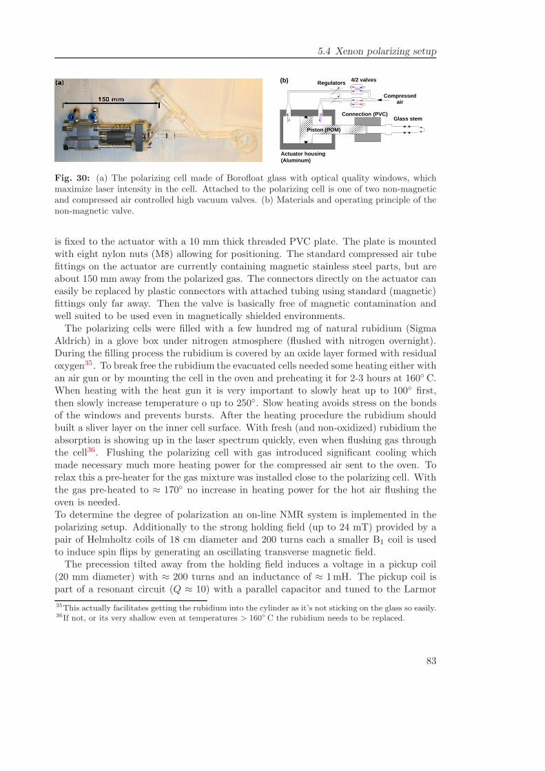
5.4 Xenon polarizing setup
(b)
Actuator housing(Aluminum)
Piston (POM)
air
4/2 valves
Compressed
Regulators
Glass stemConnection (PVC)
Fig. 30: (a) The polarizing cell made of Borofloat glass with optical quality windows, whichmaximize laser intensity in the cell. Attached to the polarizing cell is one of two non-magneticand compressed air controlled high vacuum valves. (b) Materials and operating principle of thenon-magnetic valve.
is fixed to the actuator with a 10 mm thick threaded PVC plate. The plate is mountedwith eight nylon nuts (M8) allowing for positioning. The standard compressed air tubefittings on the actuator are currently containing magnetic stainless steel parts, but areabout 150 mm away from the polarized gas. The connectors directly on the actuator caneasily be replaced by plastic connectors with attached tubing using standard (magnetic)fittings only far away. Then the valve is basically free of magnetic contamination andwell suited to be used even in magnetically shielded environments.
The polarizing cells were filled with a few hundred mg of natural rubidium (SigmaAldrich) in a glove box under nitrogen atmosphere (flushed with nitrogen overnight).During the filling process the rubidium is covered by an oxide layer formed with residualoxygen35. To break free the rubidium the evacuated cells needed some heating either withan air gun or by mounting the cell in the oven and preheating it for 2-3 hours at 160 C.When heating with the heat gun it is very important to slowly heat up to 100 first,then slowly increase temperature o up to 250. Slow heating avoids stress on the bondsof the windows and prevents bursts. After the heating procedure the rubidium shouldbuilt a sliver layer on the inner cell surface. With fresh (and non-oxidized) rubidium theabsorption is showing up in the laser spectrum quickly, even when flushing gas throughthe cell36. Flushing the polarizing cell with gas introduced significant cooling whichmade necessary much more heating power for the compressed air sent to the oven. Torelax this a pre-heater for the gas mixture was installed close to the polarizing cell. Withthe gas pre-heated to ≈ 170 no increase in heating power for the hot air flushing theoven is needed.To determine the degree of polarization an on-line NMR system is implemented in thepolarizing setup. Additionally to the strong holding field (up to 24 mT) provided by apair of Helmholtz coils of 18 cm diameter and 200 turns each a smaller B1 coil is usedto induce spin flips by generating an oscillating transverse magnetic field.
The precession tilted away from the holding field induces a voltage in a pickup coil(20 mm diameter) with ≈ 200 turns and an inductance of ≈ 1mH. The pickup coil ispart of a resonant circuit (Q ≈ 10) with a parallel capacitor and tuned to the Larmor
35This actually facilitates getting the rubidium into the cylinder as it’s not sticking on the glass so easily.36If not, or its very shallow even at temperatures > 160 C the rubidium needs to be replaced.
83
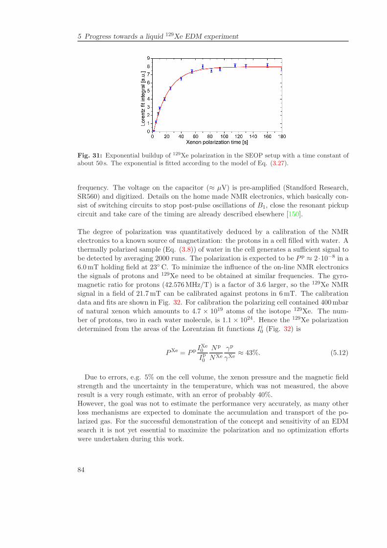
5 Progress towards a liquid 129Xe EDM experiment
Fig. 31: Exponential buildup of 129Xe polarization in the SEOP setup with a time constant ofabout 50 s. The exponential is fitted according to the model of Eq. (3.27).
frequency. The voltage on the capacitor (≈ µV) is pre-amplified (Standford Research,SR560) and digitized. Details on the home made NMR electronics, which basically con-sist of switching circuits to stop post-pulse oscillations of B1, close the resonant pickupcircuit and take care of the timing are already described elsewhere [150].
The degree of polarization was quantitatively deduced by a calibration of the NMRelectronics to a known source of magnetization: the protons in a cell filled with water. Athermally polarized sample (Eq. (3.8)) of water in the cell generates a sufficient signal tobe detected by averaging 2000 runs. The polarization is expected to be P p ≈ 2·10−8 in a6.0mT holding field at 23 C. To minimize the influence of the on-line NMR electronicsthe signals of protons and 129Xe need to be obtained at similar frequencies. The gyro-magnetic ratio for protons (42.576MHz/T) is a factor of 3.6 larger, so the 129Xe NMRsignal in a field of 21.7mT can be calibrated against protons in 6mT. The calibrationdata and fits are shown in Fig. 32. For calibration the polarizing cell contained 400mbarof natural xenon which amounts to 4.7 × 10¹⁹ atoms of the isotope 129Xe. The num-ber of protons, two in each water molecule, is 1.1 × 1024. Hence the 129Xe polarizationdetermined from the areas of the Lorentzian fit functions Ii0 (Fig. 32) is
PXe = P p IXe0
Ip0
Np
NXe
γp
γXe≈ 43%. (5.12)
Due to errors, e.g. 5% on the cell volume, the xenon pressure and the magnetic fieldstrength and the uncertainty in the temperature, which was not measured, the aboveresult is a very rough estimate, with an error of probably 40%.However, the goal was not to estimate the performance very accurately, as many otherloss mechanisms are expected to dominate the accumulation and transport of the po-larized gas. For the successful demonstration of the concept and sensitivity of an EDMsearch it is not yet essential to maximize the polarization and no optimization effortswere undertaken during this work.
84
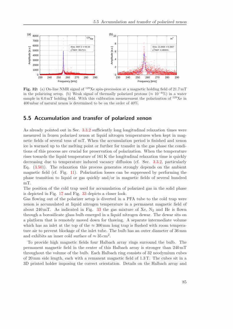
5.5 Accumulation and transfer of polarized xenon
0
1000
2000
3000
4000
5000
6000
7000
8000
230 240 250 260 270 280 290
Am
plitu
de [a
.u.]
Frequency [kHz]
(a)129Xe
Area: 3407.2 +/-50.33
χ2/NDF: 39175.5
0
2
4
6
8
10
230 240 250 260 270 280 290
Am
plitu
de [a
.u.]
Frequency [kHz]
(b)
H+
Area: 13.2656 +/-0.3837
χ2/NDF: 0.480031
Fig. 32: (a) On-line NMR signal of 129Xe spin-precession at a magnetic holding field of 21.7mTin the polarizing setup. (b) Weak signal of thermally polarized protons (≈ 10−6%) in a watersample in 6.0mT holding field. With this calibration measurement the polarization of 129Xe in400mbar of natural xenon is determined to be on the order of 40%.
5.5 Accumulation and transfer of polarized xenon
As already pointed out in Sec. 3.3.2 sufficiently long longitudinal relaxation times weremeasured in frozen polarized xenon at liquid nitrogen temperatures when kept in mag-netic fields of several tens of mT. When the accumulation period is finished and xenonice is warmed up to the melting point or further for transfer in the gas phase the condi-tions of this process are crucial for preservation of polarization. When the temperaturerises towards the liquid temperature of 161K the longitudinal relaxation time is quicklydecreasing due to temperature induced vacancy diffusion (cf. Sec. 3.3.2, particularlyEq. (3.50)). The relaxation this process generates strongly depends on the ambientmagnetic field (cf. Fig. 11). Polarization losses can be suppressed by performing thephase transition to liquid or gas quickly and/or in magnetic fields of several hundredmT.The position of the cold trap used for accumulation of polarized gas in the solid phaseis depicted in Fig. 17 and Fig. 33 depicts a closer look.Gas flowing out of the polarizer setup is diverted in a PFA tube to the cold trap werexenon is accumulated at liquid nitrogen temperature in a permanent magnetic field ofabout 240mT. As indicated in Fig. 33 the gas mixture of Xe, N2 and He is flownthrough a borosilicate glass bulb emerged in a liquid nitrogen dewar. The dewar sits ona platform that is remotely moved down for thawing. A separate intermediate volumewhich has an inlet at the top of the ≈ 300mm long trap is flushed with room tempera-ture air to prevent blockage of the inlet tube. The bulb has an outer diameter of 36mmand exhibits an inner cold surface of ≈ 35 cm2.
To provide high magnetic fields four Halbach array rings surround the bulb. Thepermanent magnetic field in the center of this Halbach array is stronger than 240mTthroughout the volume of the bulb. Each Halbach ring consists of 32 neodymium cubesof 20mm side length, each with a remanent magnetic field of 1.3T. The cubes sit in a3D printed holder imposing the correct orientation. Details on the Halbach array and
85
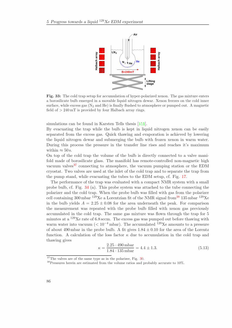
5 Progress towards a liquid 129Xe EDM experiment
N 2
LN 2
Hal
bach
arr
ay
Hal
bach
arr
ay
Air
HeXe
B=240mT
Liftingstage
Fig. 33: The cold trap setup for accumulation of hyper-polarized xenon. The gas mixture entersa borosilicate bulb emerged in a movable liquid nitrogen dewar. Xenon freezes on the cold innersurface, while excess gas (N2 and He) is finally flushed to atmosphere or pumped out. A magneticfield of > 240mT is provided by four Halbach array rings.
simulations can be found in Karsten Tells thesis [151].By evacuating the trap while the bulb is kept in liquid nitrogen xenon can be easilyseparated from the excess gas. Quick thawing and evaporation is achieved by loweringthe liquid nitrogen dewar and submerging the bulb with frozen xenon in warm water.During this process the pressure in the transfer line rises and reaches it’s maximumwithin ≈ 50 s.On top of the cold trap the volume of the bulb is directly connected to a valve mani-fold made of borosilicate glass. The manifold has remote-controlled non-magnetic highvacuum valves37 connecting to atmosphere, the vacuum pumping station or the EDMcryostat. Two valves are used at the inlet of the cold trap and to separate the trap fromthe pump stand, while evacuating the tubes to the EDM setup, cf. Fig. 17.
The performance of the trap was evaluated with a compact NMR system with a smallprobe bulb, cf. Fig. 34 (a). This probe system was attached to the tube connecting thepolarizer and the cold trap. When the probe bulb was filled with gas from the polarizercell containing 300mbar 129Xe a Lorentzian fit of the NMR signal from38 135mbar 129Xein the bulb yields A = 2.25 ± 0.08 for the area underneath the peak. For comparisonthe measurement was repeated with the probe bulb filled with xenon gas previouslyaccumulated in the cold trap. The same gas mixture was flown through the trap for 5minutes at a 129Xe rate of 6.8 sccm. The excess gas was pumped out before thawing withwarm water into vacuum (< 10−4 mbar). The accumulated 129Xe amounts to a pressureof about 490mbar in the probe bulb. A fit gives 1.84 ± 0.10 for the area of the Lorentzfunction. A calculation of the loss factor κ due to accumulation in the cold trap andthawing gives
κ =2.25 · 490mbar
1.84 · 135mbar= 4.4 ± 1.3. (5.13)
37The valves are of the same type as in the polarizer, Fig. 30.38Pressures herein are estimated from the volume ratios and probably accurate to 10%.
86
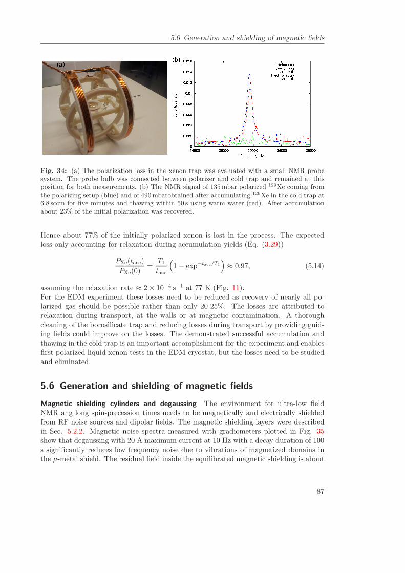
5.6 Generation and shielding of magnetic fields
Fig. 34: (a) The polarization loss in the xenon trap was evaluated with a small NMR probesystem. The probe bulb was connected between polarizer and cold trap and remained at thisposition for both measurements. (b) The NMR signal of 135mbar polarized 129Xe coming fromthe polarizing setup (blue) and of 490mbarobtained after accumulating 129Xe in the cold trap at6.8 sccm for five minutes and thawing within 50 s using warm water (red). After accumulationabout 23% of the initial polarization was recovered.
Hence about 77% of the initially polarized xenon is lost in the process. The expectedloss only accounting for relaxation during accumulation yields (Eq. (3.29))
PXe(tacc)
PXe(0)=
T1tacc
(1− exp−tacc/T1
)≈ 0.97, (5.14)
assuming the relaxation rate ≈ 2× 10⁻⁴ s−1 at 77 K (Fig. 11).For the EDM experiment these losses need to be reduced as recovery of nearly all po-larized gas should be possible rather than only 20-25%. The losses are attributed torelaxation during transport, at the walls or at magnetic contamination. A thoroughcleaning of the borosilicate trap and reducing losses during transport by providing guid-ing fields could improve on the losses. The demonstrated successful accumulation andthawing in the cold trap is an important accomplishment for the experiment and enablesfirst polarized liquid xenon tests in the EDM cryostat, but the losses need to be studiedand eliminated.
5.6 Generation and shielding of magnetic fields
Magnetic shielding cylinders and degaussing The environment for ultra-low fieldNMR ang long spin-precession times needs to be magnetically and electrically shieldedfrom RF noise sources and dipolar fields. The magnetic shielding layers were describedin Sec. 5.2.2. Magnetic noise spectra measured with gradiometers plotted in Fig. 35show that degaussing with 20 A maximum current at 10 Hz with a decay duration of 100s significantly reduces low frequency noise due to vibrations of magnetized domains inthe µ-metal shield. The residual field inside the equilibrated magnetic shielding is about
87
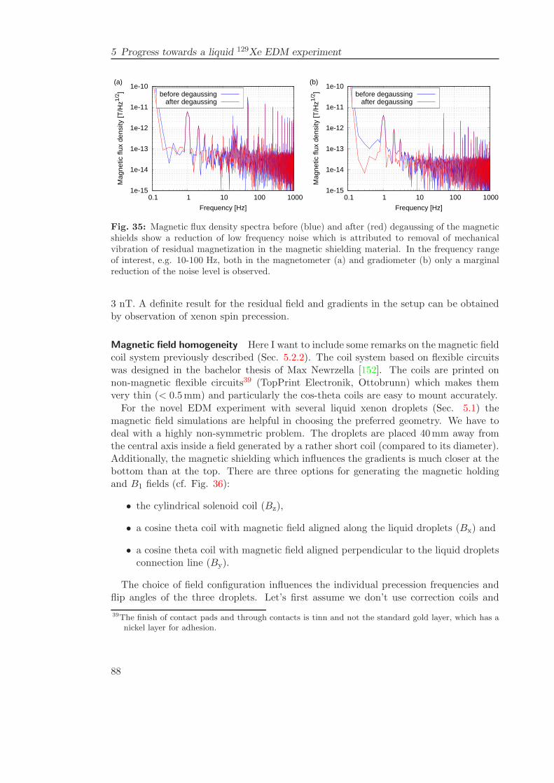
5 Progress towards a liquid 129Xe EDM experiment
1e-15
1e-14
1e-13
1e-12
1e-11
1e-10
0.1 1 10 100 1000
(a)
Mag
netic
flux
den
sity
[T/H
z1/2 ]
Frequency [Hz]
before degaussingafter degaussing
1e-15
1e-14
1e-13
1e-12
1e-11
1e-10
0.1 1 10 100 1000
(b)
Mag
netic
flux
den
sity
[T/H
z1/2 ]
Frequency [Hz]
before degaussingafter degaussing
Fig. 35: Magnetic flux density spectra before (blue) and after (red) degaussing of the magneticshields show a reduction of low frequency noise which is attributed to removal of mechanicalvibration of residual magnetization in the magnetic shielding material. In the frequency rangeof interest, e.g. 10-100 Hz, both in the magnetometer (a) and gradiometer (b) only a marginalreduction of the noise level is observed.
3 nT. A definite result for the residual field and gradients in the setup can be obtainedby observation of xenon spin precession.
Magnetic field homogeneity Here I want to include some remarks on the magnetic fieldcoil system previously described (Sec. 5.2.2). The coil system based on flexible circuitswas designed in the bachelor thesis of Max Newrzella [152]. The coils are printed onnon-magnetic flexible circuits39 (TopPrint Electronik, Ottobrunn) which makes themvery thin (< 0.5mm) and particularly the cos-theta coils are easy to mount accurately.
For the novel EDM experiment with several liquid xenon droplets (Sec. 5.1) themagnetic field simulations are helpful in choosing the preferred geometry. We have todeal with a highly non-symmetric problem. The droplets are placed 40mm away fromthe central axis inside a field generated by a rather short coil (compared to its diameter).Additionally, the magnetic shielding which influences the gradients is much closer at thebottom than at the top. There are three options for generating the magnetic holdingand B1 fields (cf. Fig. 36):
• the cylindrical solenoid coil (Bz),
• a cosine theta coil with magnetic field aligned along the liquid droplets (Bx) and
• a cosine theta coil with magnetic field aligned perpendicular to the liquid dropletsconnection line (By).
The choice of field configuration influences the individual precession frequencies andflip angles of the three droplets. Let’s first assume we don’t use correction coils and
39The finish of contact pads and through contacts is tinn and not the standard gold layer, which has anickel layer for adhesion.
88
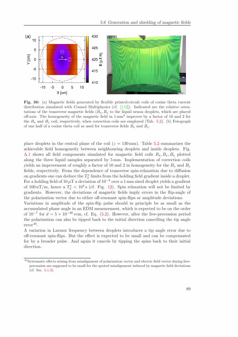
5.6 Generation and shielding of magnetic fields
Fig. 36: (a) Magnetic fields generated by flexible printed-circuit coils of cosine theta currentdistribution simulated with Comsol Multiphysics (cf. [152]). Indicated are the relative orien-tations of the transverse magnetic fields (Bx, By to the liquid xenon droplets, which are placedoff-axis. The homogeneity of the magnetic field in 1mm3 improves by a factor of 10 and 2 forthe Bx and By coil, respectively, when correction coils are employed (Tab. 5.2). (b) Fotographof one half of a cosine theta coil as used for transverse fields Bx and By.
place droplets in the central plane of the coil (z = 130mm). Table 5.2 summarizes theachievable field homogeneity between neighbouring droplets and inside droplets. Fig.A.1 shows all field components simulated for magnetic field coils Bx, By, Bz plottedalong the three liquid samples separated by 5mm. Implementation of correction coilsyields an improvement of roughly a factor of 10 and 2 in homogeneity for the Bx and By
fields, respectively. From the dependence of transverse spin-relaxation due to diffusionon gradients one can deduce the T ∗
2 limits from the holding field gradient inside a droplet.For a holding field of 10µT a deviation of 10−4 over a 1mm sized droplet yields a gradientof 100 nT/m, hence a T ∗
2 < 104 s (cf. Fig. 12). Spin relaxation will not be limited bygradients. However, the deviations of magnetic fields imply errors in the flip-angle ofthe polarization vector due to either off-resonant spin-flips or amplitude deviations.Variations in amplitude of the spin-flip pulse should in principle be as small as theaccumulated phase angle in an EDM measurement, which is expected to be on the orderof 10−7 for d = 5 × 10⁻³⁰ ecm, cf. Eq. (5.2). However, after the free-precession periodthe polarization can also be tipped back to the initial direction cancelling the tip angleerror40.A variation in Larmor frequency between droplets introduces a tip angle error due tooff-resonant spin-flips. But the effect is expected to be small and can be compensatedfor by a broader pulse. And again it cancels by tipping the spins back to their initialdirection.
40Systematic effects arising from misalignment of polarization vector and electric field vector during free-precession are supposed to be small for the quoted misalignment induced by magnetic field deviations(cf. Sec. 5.1.3).
89
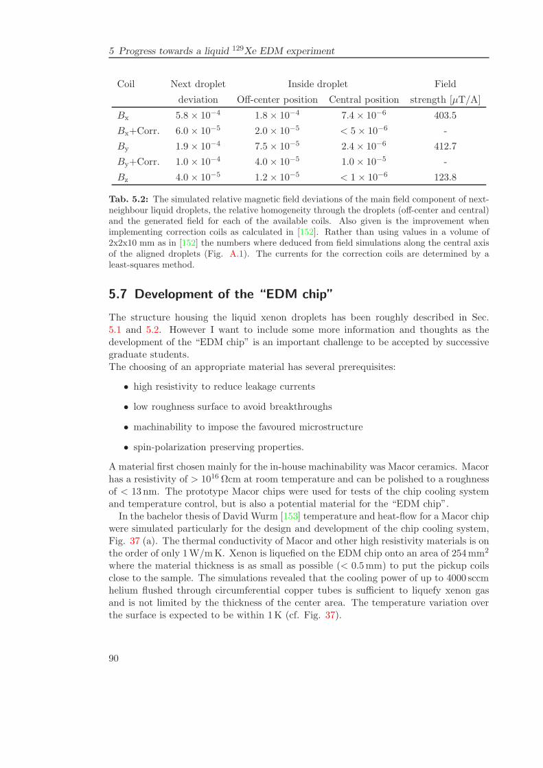
5 Progress towards a liquid 129Xe EDM experiment
Coil Next droplet Inside droplet Field
deviation Off-center position Central position strength [µT/A]
Bx 5.8 × 10⁻⁴ 1.8× 10⁻⁴ 7.4× 10⁻⁶ 403.5
Bx+Corr. 6.0 × 10⁻⁵ 2.0× 10⁻⁵ < 5× 10⁻⁶ -
By 1.9 × 10⁻⁴ 7.5× 10⁻⁵ 2.4× 10⁻⁶ 412.7
By+Corr. 1.0 × 10⁻⁴ 4.0× 10⁻⁵ 1.0× 10⁻⁵ -
Bz 4.0 × 10⁻⁵ 1.2× 10⁻⁵ < 1× 10⁻⁶ 123.8
Tab. 5.2: The simulated relative magnetic field deviations of the main field component of next-neighbour liquid droplets, the relative homogeneity through the droplets (off-center and central)and the generated field for each of the available coils. Also given is the improvement whenimplementing correction coils as calculated in [152]. Rather than using values in a volume of2x2x10 mm as in [152] the numbers where deduced from field simulations along the central axisof the aligned droplets (Fig. A.1). The currents for the correction coils are determined by aleast-squares method.
5.7 Development of the “EDM chip”
The structure housing the liquid xenon droplets has been roughly described in Sec.5.1 and 5.2. However I want to include some more information and thoughts as thedevelopment of the “EDM chip” is an important challenge to be accepted by successivegraduate students.The choosing of an appropriate material has several prerequisites:
• high resistivity to reduce leakage currents
• low roughness surface to avoid breakthroughs
• machinability to impose the favoured microstructure
• spin-polarization preserving properties.
A material first chosen mainly for the in-house machinability was Macor ceramics. Macorhas a resistivity of > 1016 Ωcm at room temperature and can be polished to a roughnessof < 13 nm. The prototype Macor chips were used for tests of the chip cooling systemand temperature control, but is also a potential material for the “EDM chip”.
In the bachelor thesis of David Wurm [153] temperature and heat-flow for a Macor chipwere simulated particularly for the design and development of the chip cooling system,Fig. 37 (a). The thermal conductivity of Macor and other high resistivity materials is onthe order of only 1W/mK. Xenon is liquefied on the EDM chip onto an area of 254mm2
where the material thickness is as small as possible (< 0.5mm) to put the pickup coilsclose to the sample. The simulations revealed that the cooling power of up to 4000 sccmhelium flushed through circumferential copper tubes is sufficient to liquefy xenon gasand is not limited by the thickness of the center area. The temperature variation overthe surface is expected to be within 1K (cf. Fig. 37).
90
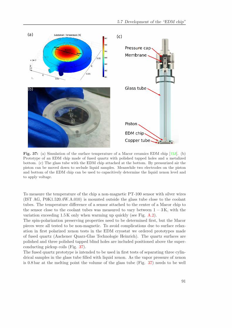
5.7 Development of the “EDM chip”
Fig. 37: (a) Simulation of the surface temperature of a Macor ceramics EDM chip [153]. (b)Prototype of an EDM chip made of fused quartz with polished tapped holes and a metalizedbottom. (c) The glass tube with the EDM chip attached at the bottom. By pressurized air thepiston can be moved down to seclude liquid samples. Meanwhile two electrodes on the pistonand bottom of the EDM chip can be used to capacitively determine the liquid xenon level andto apply voltage.
To measure the temperature of the chip a non-magnetic PT-100 sensor with silver wires(IST AG, P0K1.520.4W.A.010) is mounted outside the glass tube close to the coolanttubes. The temperature difference of a sensor attached to the center of a Macor chip tothe sensor close to the coolant tubes was measured to vary between 1 − 3K, with thevariation exceeding 1.5K only when warming up quickly (see Fig. A.2).The spin-polarization preserving properties need to be determined first, but the Macorpieces were all tested to be non-magnetic. To avoid complications due to surface relax-ation in first polarized xenon tests in the EDM cryostat we ordered prototypes madeof fused quartz (Aachener Quarz-Glas Technologie Heinrich). The quartz surfaces arepolished and three polished tapped blind holes are included positioned above the super-conducting pickup coils (Fig. 37).The fused quartz prototype is intended to be used in first tests of separating three cylin-drical samples in the glass tube filled with liquid xenon. As the vapor pressure of xenonis 0.8 bar at the melting point the volume of the glass tube (Fig. 37) needs to be well
91
5 Progress towards a liquid 129Xe EDM experiment
sealed to the surrounding vacuum41. The EDM chip is glued to the glass tube end withepoxy glue (Hysol C1, Henkel), which is known to be non-magnetic and polarizationpreserving.The three blind holes of the prototype chip can be secluded by a lid, whereas a morecomplicated development will follow for employing three spherical volumes as the shapeof highest symmetry. With the pickup coils underneath individual spin precession ofeach separated volume can be studied. The mechanism to move a piston to later enclosesamples is already developed and operable. It also serves the purpose of determining theamount of liquid xenon. In the thesis of Karsten Tell [151] the feasibility of a capacitivemeasurement of the liquid xenon level was demonstrated by using a movable electrode.Compressed air is used to deflect the piston attached to a membrane which was mountedon top of the glass tube, cf. Fig. 37 (c). The metalized bottom of the EDM chip actsas one electrode while the second electrode is the metalized bottom of the piston. Thepiston can be moved down with liquid xenon filled and hence close the liquid samplesswamping out excess liquid. This mechanism is ready to be implemented in the EDMsetup and enables observation of individual polarized liquid samples, which is easier torealize than spherical samples. Nevertheless, the influence on spin-relaxation times asto be determined.The two electrodes are also available to apply voltage to a liquid sample and test thehigh voltage behaviour of the setup. For application of rotating electric fields electrodessurrounding each droplet need to be implemented in the “EDM chip”.
5.8 Summary of the liquid xenon EDM experiment
The new liquid xenon EDM experiment is now in a status of being ready to studyspin-relaxation in liquid xenon and determine the sensitivity achievable in an EDM ex-periment.The potential gain of using a liquid sample motivates the challenging R&D work. Thepaper draft presented in Sec. 5.1 describes the novel method introducing time-varyingelectric fields in an EDM search and several new subsequent systematic effects. Mostof which seem to be in control, but predominantly AC leakage currents arising fromthe electrode capacitance seem to limit the sensitivity if the electric field is not per-fectly aligned at 90 to the precessing polarization vector. Nevertheless, with a feasiblealignment accuracy and a reference experiment the EDM sensitivity can be significantlyimproved over the current limit.In the course of this work it turned out be be more difficult to reliably operate thedetection system of superconducting pickup loops and SQUIDs in a cryogen free setup.Particularly with implementation of the “EDM chip” and it’s cooling system, whichintroduces a significant radiative heat source. Due to magnetic shielding space for feed-through of the vacuum system and the cross-sectional area for thermal connection to
41It is actually not a trivial task to find the right glue as the epoxy seal has to withstand 1 bar of over-pressure, while the temperature of the chip cycles between 90 K and 250 K. The thermal expansioncoefficients of glass and typical epoxy glues deviate significantly.
92
5.8 Summary of the liquid xenon EDM experiment
the coldhead is very limited. However, all cryogenic issues were solved and the residualheat load was successfully removed to be marginal. Significant radiative heating comesfrom the “EDM chip” and helium cooling line which is now limiting the operating rangeof the superconducting pickup coils to . 180K. Finally, in this range the noise floorof a gradiometer pickup coil is 144 fT/
√Hz above 50Hz, even with a sample on the
“EDM chip” at 162K. The most dominant peaks are from vibration due to the movingcoldhead piston and the power line frequency. The low frequency peaks from vibrationsare of less concern in NMR measurements, whereas the strong 50Hz signal is closerto spin-precession frequencies and potentially introduces spin-flips. One future task isfinding and eliminating the sources of this peak and increasing the noise performance ofthe setup.Parts of the liquid xenon EDM setup regarding production of large amounts of hyper-polarized xenon and transfer were built from scratch during this thesis. It was demon-strated that these components perform well and reliably deliver the polarized gas to beliquefied in the EDM setup. Improvements and optimizations of production parametersand reduction of losses during accumulation and transport need to be addressed in thefuture but are not limiting at this stage.The possible approaches to deliver polarized liquid to the EDM setup have been eval-uated. Accumulation of the polarized gas by freezing to the “EDM chip” suffers fromsevere polarization losses in elevated temperatures and low magnetic fields (cf. Sec.3.3.2). As only small magnetic fields are available in the setup the warming and thawingneeds to be done very quickly. However, due to the heat capacity and heat conductivityof the “EDM chip” material the heating process is slow (Fig. 24). Directly liquefyingxenon from gas phase seems to be the best way and successful liquefaction on the “EDMchip” was already observed.A major step to implementation of time-varying electric fields is the development of the“EDM chip” with electrodes introduced around the droplet cavities. But, already nowan implementation of electrodes for a constant electric field along the magnetic holdingfield is nearly completed and a Ramsey-type EDM experiment is rather straightforwardas soon as spin-precession can be observed.The sensitivity will strongly depend on the preserved polarization and transverse spinrelaxation times. These need to be experimentally determined in the setup to deducean estimate on the EDM sensitivity accessible in the near future.The setup now offers a rich playground probably for generations of graduate students tostudy spin-relaxation in low fields and explore the potential of novel methods of a liquidxenon EDM search.
93

6 A new EDM experiment using a He/Xemixture and SQUID detection
As already pointed out earlier (cf. Sec. 2.5, Tab. 2.7) even slight improvements ofdXe to about 10−28 ecm will give enough information additional to the superior 199HgEDM measurement to get further insight and to better constrain several coefficients ofCP violating interactions. This can potentially be achieved by improving the “conven-tional” method used in EDM searches with parallel electric and magnetic fields. Besidesusing a co-magnetometer as in [71] (cf. Sec. 4.1), two main features account for anexpected improvement of EDM sensitivity. The use of a very low noise detection systemyields a high signal-to-noise ratio even at low pressures. Observation time of 3He spinprecession at pressures of 1000mbar is mostly limited by magnetic field gradients, whilefor 100mbar of 129Xe wall collisions are more dominant.In an EDM measurement the electric field is sequentially reversed, while keeping themagnetic field, which cancels the Zeeman term in first order. However, a false EDMsignal arises if an additional magnetic field is generated, that reverses sign with the elec-tric field. The usually relevant geometric phase effect due to motional magnetic fields(∝ v ×E) is of no concern at high pressures, since the Larmor period τL is much largerthan the correlation time τc (cf. [30]). The commonly most dominant effect due toleakage currents will be accounted for by the 3He co-magnetometer that doesn’t have anEDM42.The continuous operation of the He-Xe maser suffered mostly from instability of elec-tronics and feedback loops as well as signal size. Our He-Xe clock comparison experimentis placed inside the Munich magnetically shielded room (MMSR) [154]. The room pro-vides a very stable, RF shielded environment with very low magnetic field gradients(. 1 nT/m) and low residual fields (≈ nT). Even more, with the inner shielding sectioninstalled it’s expected to be the world’s best magnetically and electrically shielded envi-ronment with a shielding factor of 106 at quasi-DC frequencies.We aim to observe spin-precession in an applied electric field for several hundred secondsin each run. To improve statistics the collaboration is developing a gas system to contin-uously refill the EDM cell with freshly polarized gas while mounted inside the MMSR.This flowing gas concept brings some challenges, particularly for a system using suchdifferent species as 3He and 129Xe. But, it will make long-term operation feasible whichcould give a statistical improvement on the order of ≈ 1000 in one year (cf. (4.6)).A question arising is the composition of the gas mixture. The only fixed pressure is thequenching gas, which will be about 100 mbar of N2. The total pressure in the EDMcell (and the closed-cycle system) should be above one atmosphere, but not limiting
42Or at least one much smaller than the anticipated sensitivity.
95
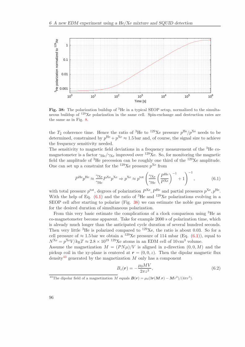
6 A new EDM experiment using a He/Xe mixture and SQUID detection
0.001
0.01
0.1
1
100 101 102 103 104 105 106
3 He
pola
rizat
ion
norm
aliz
ed to
129 X
e
Time [s]
Fig. 38: The polarization buildup of 3He in a typical SEOP setup, normalized to the simulta-neous buildup of 129Xe polarization in the same cell. Spin-exchange and destruction rates arethe same as in Fig. 8.
the T2 coherence time. Hence the ratio of 3He to 129Xe pressure pHe/pXe needs to bedetermined, constrained by pHe + pXe ≈ 1.5 bar and, of course, the signal size to achievethe frequency sensitivity needed.The sensitivity to magnetic field deviations in a frequency measurement of the 3He co-magnetometer is a factor γHe/γXe improved over 129Xe. So, for monitoring the magneticfield the amplitude of 3He precession can be roughly one third of the 129Xe amplitude.One can set up a constraint for the 129Xe pressure pXe from
PHepHe ≈ γXe
γHePXepXe ⇒ pXe ≈ ptot
(γXe
γHe
(PHe
PXe
)−1
+ 1
)−1
, (6.1)
with total pressure ptot, degrees of polarization PXe, PHe and partial pressures pXe, pHe.With the help of Eq. (6.1) and the ratio of 3He and 129Xe polarizations evolving in aSEOP cell after starting to polarize (Fig. 38) we can estimate the noble gas pressuresfor the desired duration of simultaneous polarization.
From this very basic estimate the complications of a clock comparison using 3He asco-magnetometer become apparent. Take for example 2000 s of polarization time, whichis already much longer than the anticipated cycle duration of several hundred seconds.Then very little 3He is polarized compared to 129Xe, the ratio is about 0.03. So for acell pressure of ≈ 1.5 bar we obtain a 129Xe pressure of 114 mbar (Eq. (6.1)), equal toNXe = pXeV/kBT ≈ 2.8× 10¹⁹ 129Xe atoms in an EDM cell of 10 cm3 volume.Assume the magnetization M = (PNµ)/V is aligned in z-direction (0, 0,M) and thepickup coil in the xy-plane is centered at r = (0, 0, z). Then the dipolar magnetic fluxdensity43 generated by the magnetization M only has a component
Bz(r) = −µ0MV
2πz3, (6.2)
43The dipolar field of a magnetization M equals B(r) = µ0(3r(M .r) −Mr2)/(4πr5).
96
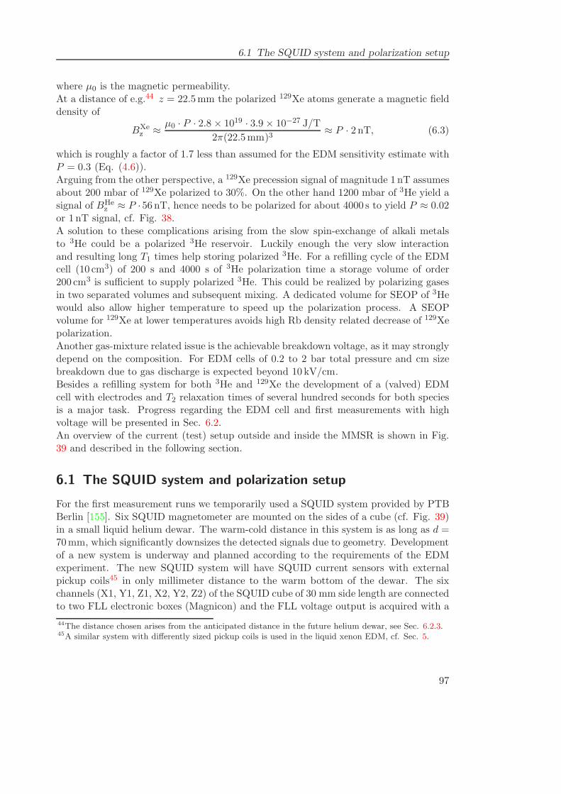
6.1 The SQUID system and polarization setup
where µ0 is the magnetic permeability.At a distance of e.g.44 z = 22.5mm the polarized 129Xe atoms generate a magnetic fielddensity of
BXez ≈ µ0 · P · 2.8 × 1019 · 3.9× 10−27 J/T
2π(22.5mm)3≈ P · 2 nT, (6.3)
which is roughly a factor of 1.7 less than assumed for the EDM sensitivity estimate withP = 0.3 (Eq. (4.6)).Arguing from the other perspective, a 129Xe precession signal of magnitude 1 nT assumesabout 200 mbar of 129Xe polarized to 30%. On the other hand 1200 mbar of 3He yield asignal of BHe
z ≈ P ·56 nT, hence needs to be polarized for about 4000 s to yield P ≈ 0.02or 1 nT signal, cf. Fig. 38.A solution to these complications arising from the slow spin-exchange of alkali metalsto 3He could be a polarized 3He reservoir. Luckily enough the very slow interactionand resulting long T1 times help storing polarized 3He. For a refilling cycle of the EDMcell (10 cm3) of 200 s and 4000 s of 3He polarization time a storage volume of order200 cm3 is sufficient to supply polarized 3He. This could be realized by polarizing gasesin two separated volumes and subsequent mixing. A dedicated volume for SEOP of 3Hewould also allow higher temperature to speed up the polarization process. A SEOPvolume for 129Xe at lower temperatures avoids high Rb density related decrease of 129Xepolarization.Another gas-mixture related issue is the achievable breakdown voltage, as it may stronglydepend on the composition. For EDM cells of 0.2 to 2 bar total pressure and cm sizebreakdown due to gas discharge is expected beyond 10 kV/cm.Besides a refilling system for both 3He and 129Xe the development of a (valved) EDMcell with electrodes and T2 relaxation times of several hundred seconds for both speciesis a major task. Progress regarding the EDM cell and first measurements with highvoltage will be presented in Sec. 6.2.An overview of the current (test) setup outside and inside the MMSR is shown in Fig.39 and described in the following section.
6.1 The SQUID system and polarization setup
For the first measurement runs we temporarily used a SQUID system provided by PTBBerlin [155]. Six SQUID magnetometer are mounted on the sides of a cube (cf. Fig. 39)in a small liquid helium dewar. The warm-cold distance in this system is as long as d =70mm, which significantly downsizes the detected signals due to geometry. Developmentof a new system is underway and planned according to the requirements of the EDMexperiment. The new SQUID system will have SQUID current sensors with externalpickup coils45 in only millimeter distance to the warm bottom of the dewar. The sixchannels (X1, Y1, Z1, X2, Y2, Z2) of the SQUID cube of 30 mm side length are connectedto two FLL electronic boxes (Magnicon) and the FLL voltage output is acquired with a
44The distance chosen arises from the anticipated distance in the future helium dewar, see Sec. 6.2.3.45A similar system with differently sized pickup coils is used in the liquid xenon EDM, cf. Sec. 5.
97
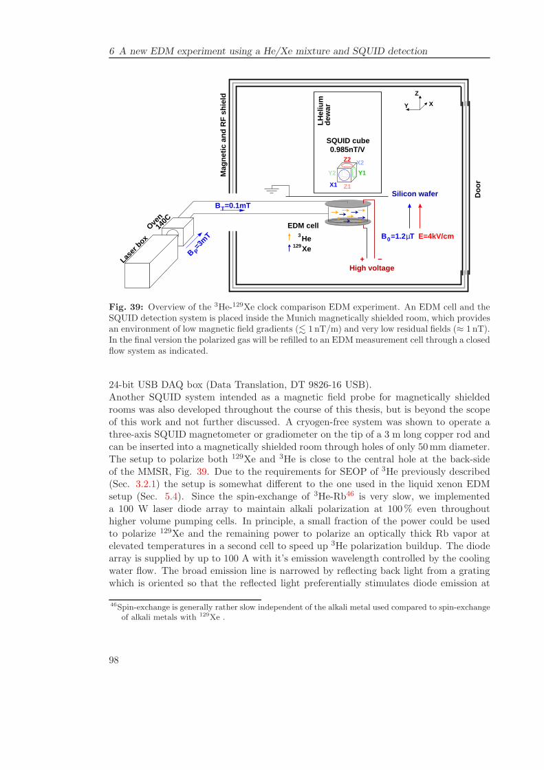
6 A new EDM experiment using a He/Xe mixture and SQUID detection
−+High voltage
dew
arLH
eliu
m
B =0.1mTT
µ
Mag
netic
and
RF
shi
eld
Doo
r
140C
Silicon wafer
EDM cell
Y2 Y1
Z1
Z2
X1
X2
SQUID cube0.985nT/V
B =3m
T
P
Oven
Y X
Z
Lase
r box
Xe129He3 B =1.2 T0 E=4kV/cm
Fig. 39: Overview of the 3He-129Xe clock comparison EDM experiment. An EDM cell and theSQUID detection system is placed inside the Munich magnetically shielded room, which providesan environment of low magnetic field gradients (. 1 nT/m) and very low residual fields (≈ 1 nT).In the final version the polarized gas will be refilled to an EDMmeasurement cell through a closedflow system as indicated.
24-bit USB DAQ box (Data Translation, DT 9826-16 USB).Another SQUID system intended as a magnetic field probe for magnetically shieldedrooms was also developed throughout the course of this thesis, but is beyond the scopeof this work and not further discussed. A cryogen-free system was shown to operate athree-axis SQUID magnetometer or gradiometer on the tip of a 3 m long copper rod andcan be inserted into a magnetically shielded room through holes of only 50mm diameter.The setup to polarize both 129Xe and 3He is close to the central hole at the back-sideof the MMSR, Fig. 39. Due to the requirements for SEOP of 3He previously described(Sec. 3.2.1) the setup is somewhat different to the one used in the liquid xenon EDMsetup (Sec. 5.4). Since the spin-exchange of 3He-Rb46 is very slow, we implementeda 100 W laser diode array to maintain alkali polarization at 100% even throughouthigher volume pumping cells. In principle, a small fraction of the power could be usedto polarize 129Xe and the remaining power to polarize an optically thick Rb vapor atelevated temperatures in a second cell to speed up 3He polarization buildup. The diodearray is supplied by up to 100 A with it’s emission wavelength controlled by the coolingwater flow. The broad emission line is narrowed by reflecting back light from a gratingwhich is oriented so that the reflected light preferentially stimulates diode emission at
46Spin-exchange is generally rather slow independent of the alkali metal used compared to spin-exchangeof alkali metals with 129Xe .
98
6.2 Progress and test measurement results
Fig. 40: (a) The setup of Helmholtz coils and SQUID dewar inside the magnetically shieldedroom used for test measurement runs. (b) The PTB glass bulb mounted underneath the SQUIDdewar. (c) Prototype EDM cell with pumping and measurement chambers. Two silicon wafersas electrodes are bonded to a glass cylinder (GE180).
794.8 nm. The emitted light is sent through the usual optics to circularly polarize thephotons and enters an oven in a round shape of about 60 mm diameter.Typical magnetic fields used for SEOP and polarized gas transport are shown in Fig.39.
6.2 Progress and test measurement results
In two test runs we made significant progress towards an upcoming EDM run. In thesubsequently following sections I will present results and their implications on the wayto an upcoming EDM run planned for 2015. First, I introduce some technical details ondata analysis and the measurement procedure.
Data analysis and fittingThe spin precession data discussed was processed the following way. The FLL elec-
tronics provide outputs for six SQUIDs mounted on the SQUID cube (Fig. 39). As allthe SQUID loops point inwards a gradiometer signal is obtained by summing SQUID
99
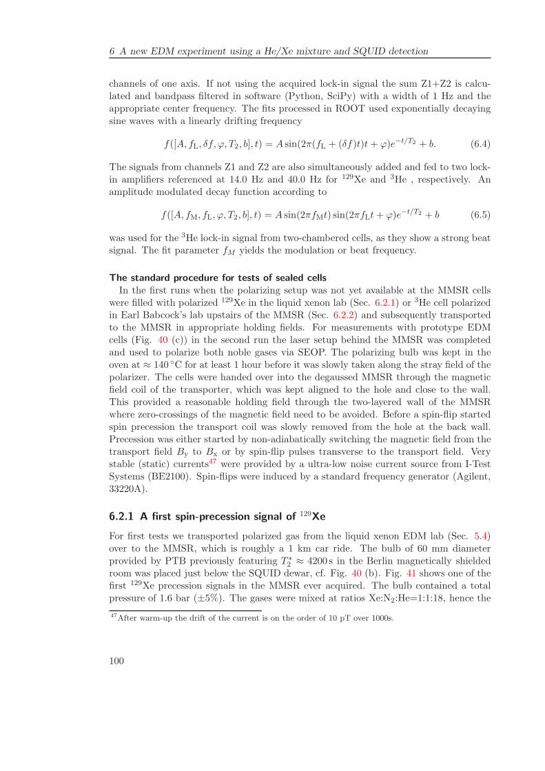
6 A new EDM experiment using a He/Xe mixture and SQUID detection
channels of one axis. If not using the acquired lock-in signal the sum Z1+Z2 is calcu-lated and bandpass filtered in software (Python, SciPy) with a width of 1 Hz and theappropriate center frequency. The fits processed in ROOT used exponentially decayingsine waves with a linearly drifting frequency
f([A, fL, δf, ϕ, T2, b], t) = A sin(2π(fL + (δf)t)t+ ϕ)e−t/T2 + b. (6.4)
The signals from channels Z1 and Z2 are also simultaneously added and fed to two lock-in amplifiers referenced at 14.0 Hz and 40.0 Hz for 129Xe and 3He , respectively. Anamplitude modulated decay function according to
f([A, fM, fL, ϕ, T2, b], t) = A sin(2πfMt) sin(2πfLt+ ϕ)e−t/T2 + b (6.5)
was used for the 3He lock-in signal from two-chambered cells, as they show a strong beatsignal. The fit parameter fM yields the modulation or beat frequency.
The standard procedure for tests of sealed cellsIn the first runs when the polarizing setup was not yet available at the MMSR cells
were filled with polarized 129Xe in the liquid xenon lab (Sec. 6.2.1) or 3He cell polarizedin Earl Babcock’s lab upstairs of the MMSR (Sec. 6.2.2) and subsequently transportedto the MMSR in appropriate holding fields. For measurements with prototype EDMcells (Fig. 40 (c)) in the second run the laser setup behind the MMSR was completedand used to polarize both noble gases via SEOP. The polarizing bulb was kept in theoven at ≈ 140 C for at least 1 hour before it was slowly taken along the stray field of thepolarizer. The cells were handed over into the degaussed MMSR through the magneticfield coil of the transporter, which was kept aligned to the hole and close to the wall.This provided a reasonable holding field through the two-layered wall of the MMSRwhere zero-crossings of the magnetic field need to be avoided. Before a spin-flip startedspin precession the transport coil was slowly removed from the hole at the back wall.Precession was either started by non-adiabatically switching the magnetic field from thetransport field By to Bx or by spin-flip pulses transverse to the transport field. Verystable (static) currents47 were provided by a ultra-low noise current source from I-TestSystems (BE2100). Spin-flips were induced by a standard frequency generator (Agilent,33220A).
6.2.1 A first spin-precession signal of 129Xe
For first tests we transported polarized gas from the liquid xenon EDM lab (Sec. 5.4)over to the MMSR, which is roughly a 1 km car ride. The bulb of 60 mm diameterprovided by PTB previously featuring T ∗
2 ≈ 4200 s in the Berlin magnetically shieldedroom was placed just below the SQUID dewar, cf. Fig. 40 (b). Fig. 41 shows one of thefirst 129Xe precession signals in the MMSR ever acquired. The bulb contained a totalpressure of 1.6 bar (±5%). The gases were mixed at ratios Xe:N2:He=1:1:18, hence the
47After warm-up the drift of the current is on the order of 10 pT over 1000s.
100
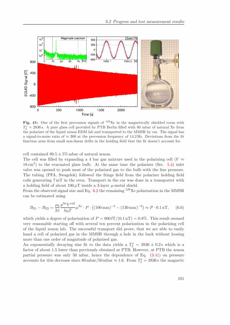
6.2 Progress and test measurement results
Fig. 41: One of the first precession signals of 129Xe in the magnetically shielded room withT ∗
2 = 2836 s. A pure glass cell provided by PTB Berlin filled with 80 mbar of natural Xe fromthe polarizer of the liquid xenon EDM lab and transported to the MMSR by car. The signal hasa signal-to-noise ratio of ≈ 300 at the precession frequency of 14.2Hz. Deviations from the fitfunction arise from small non-linear drifts in the holding field that the fit doesn’t account for.
cell contained 80.5 ± 5%mbar of natural xenon.The cell was filled by expanding a 4 bar gas mixture used in the polarizing cell (V ≈18 cm3) to the evacuated glass bulb. At the same time the polarizer (Sec. 5.4) inletvalve was opened to push most of the polarized gas to the bulb with the line pressure.The tubing (PFA, Swagelok) followed the fringe field from the polarizer holding fieldcoils generating 7mT in the oven. Transport in the car was done in a transporter witha holding field of about 100µT inside a 3-layer µ-metal shield.From the observed signal size and Eq. 6.2 the remaining 129Xe polarization in the MMSRcan be estimated using
BZ1 −BZ2 =µ02π
pXeV cell
kBTµXe · P ·
((100mm)−3 − (130mm)−3
)≈ P · 0.1 nT, (6.6)
which yields a degree of polarization of P = 800 fT/(0.1 nT) = 0.8%. This result seemedvery reasonable starting off with several ten percent polarization in the polarizing cellof the liquid xenon lab. The successful transport did prove, that we are able to easilyhand a cell of polarized gas in the MMSR through a hole in the back without loosingmore than one order of magnitude of polarized gas.An exponentially decaying sine fit to the data yields a T ∗
2 = 2836 ± 0.2 s which is afactor of about 1.5 lower than previously obtained at PTB. However, at PTB the xenonpartial pressure was only 50 mbar, hence the dependence of Eq. (3.41) on pressureaccounts for this decrease since 80mbar/50mbar ≈ 1.6. From T ∗
2 = 2836 s the magnetic
101
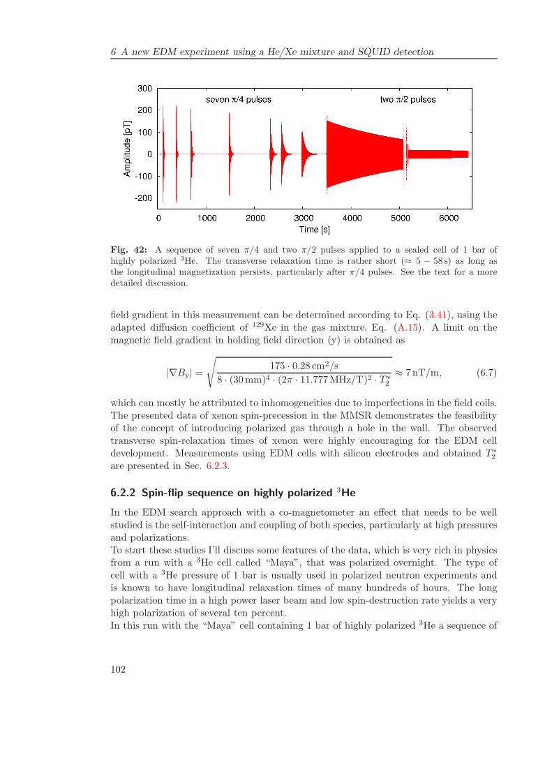
6 A new EDM experiment using a He/Xe mixture and SQUID detection
Fig. 42: A sequence of seven π/4 and two π/2 pulses applied to a sealed cell of 1 bar ofhighly polarized 3He. The transverse relaxation time is rather short (≈ 5 − 58 s) as long asthe longitudinal magnetization persists, particularly after π/4 pulses. See the text for a moredetailed discussion.
field gradient in this measurement can be determined according to Eq. (3.41), using theadapted diffusion coefficient of 129Xe in the gas mixture, Eq. (A.15). A limit on themagnetic field gradient in holding field direction (y) is obtained as
|∇By| =√
175 · 0.28 cm2/s
8 · (30mm)4 · (2π · 11.777MHz/T)2 · T ∗2
≈ 7 nT/m, (6.7)
which can mostly be attributed to inhomogeneities due to imperfections in the field coils.The presented data of xenon spin-precession in the MMSR demonstrates the feasibilityof the concept of introducing polarized gas through a hole in the wall. The observedtransverse spin-relaxation times of xenon were highly encouraging for the EDM celldevelopment. Measurements using EDM cells with silicon electrodes and obtained T ∗
2
are presented in Sec. 6.2.3.
6.2.2 Spin-flip sequence on highly polarized 3He
In the EDM search approach with a co-magnetometer an effect that needs to be wellstudied is the self-interaction and coupling of both species, particularly at high pressuresand polarizations.To start these studies I’ll discuss some features of the data, which is very rich in physicsfrom a run with a 3He cell called “Maya”, that was polarized overnight. The type ofcell with a 3He pressure of 1 bar is usually used in polarized neutron experiments andis known to have longitudinal relaxation times of many hundreds of hours. The longpolarization time in a high power laser beam and low spin-destruction rate yields a veryhigh polarization of several ten percent.In this run with the “Maya” cell containing 1 bar of highly polarized 3He a sequence of
102
6.2 Progress and test measurement results
seven π/4 and two π/2 spin-flip pulses was applied. In-between pulses the transversemagnetization was destroyed by applying a magnetic field gradient. Fig. 42 shows thebandpass filtered Z gradiometer signal of this run.
Off-resonant spin-flipsClearly the T ∗
2 time grows as subsequent pulses are applied and is much longer afterthe last two π/2 pulses. Since the T1 time is at least on the order of tens of hours thedecrease in longitudinal magnetization due to relaxation can be neglected.A first obvious feature of the data is, that the inital amplitudes only decrease slightly,although a loss of longitudinal magnetization of roughly sin(π/4) = 1/
√2 is expected
for each spin-flip. In contrast to a perfectly spherical cell, the magnetization in thecylindrical cell (≈ 100mm diameter, 50mm height) of ≈ 400 cm3 volume (1021 polarizedatoms) generates an intrinsic local magnetic field of order 500 nT. In a holding fieldof only 1.2µT this amounts to 10%, which renders the spin-flip pulse off-resonant andinefficient.The actual gradiometer signal expected after a π/4 flip is on the order of
S =1√2
µ02π
· 1021 · µHe ·((120mm)3 − (150mm3)
)≈ 400 pT. (6.8)
From this rough estimate the spin-flip efficiency is about 1/2.
Spin-flip accuracyFrom the two datasets following the π/2 pulses the accuracy of the spin-flips can be
determined. The (small) error in flip-angle is δθ ≈ δa/a0, where a0 is the initial magne-tization and δa0 the remaining longitudinal magnetization. The ratio of the amplitudesof subsequent π/2 pulses gives the error in flip angle
a1a2
=a0√1 + δθ2
δa√1 + δθ2
=1
δθ. (6.9)
The amplitudes from the fitted decaying sine functions yield δθ = 0.13248 (±5.2×10⁻⁵),hence an accuracy of an applied 90 pulse of 7.6 or about 10%.
Dipolar gradient limited transverse relaxationAlso clearly indicated is an increase of T ∗
2 as longitudinal magnetization is subse-quently reduced and becomes much longer after the π/2 pulses. This indicates, that thegradient due to the dipolar field of the longitudinal magnetization vanishes and is notlimiting T ∗
2 any more.The initial amplitudes and precession frequencies of the free induction decays are ob-tained by fitting decaying sine functions (see Fig. 43 (b) for an example). The transverserelaxation time is expected to obey a inverse-square law dependence on the initial am-plitude and frequency of the free induction decay (Fig. 43) as T−1
2 ∝ |∇Bz|2 ∝ B2 ∝M2(Eq. (3.41)). The observed initial precession amplitudes and precession frequencies of
103
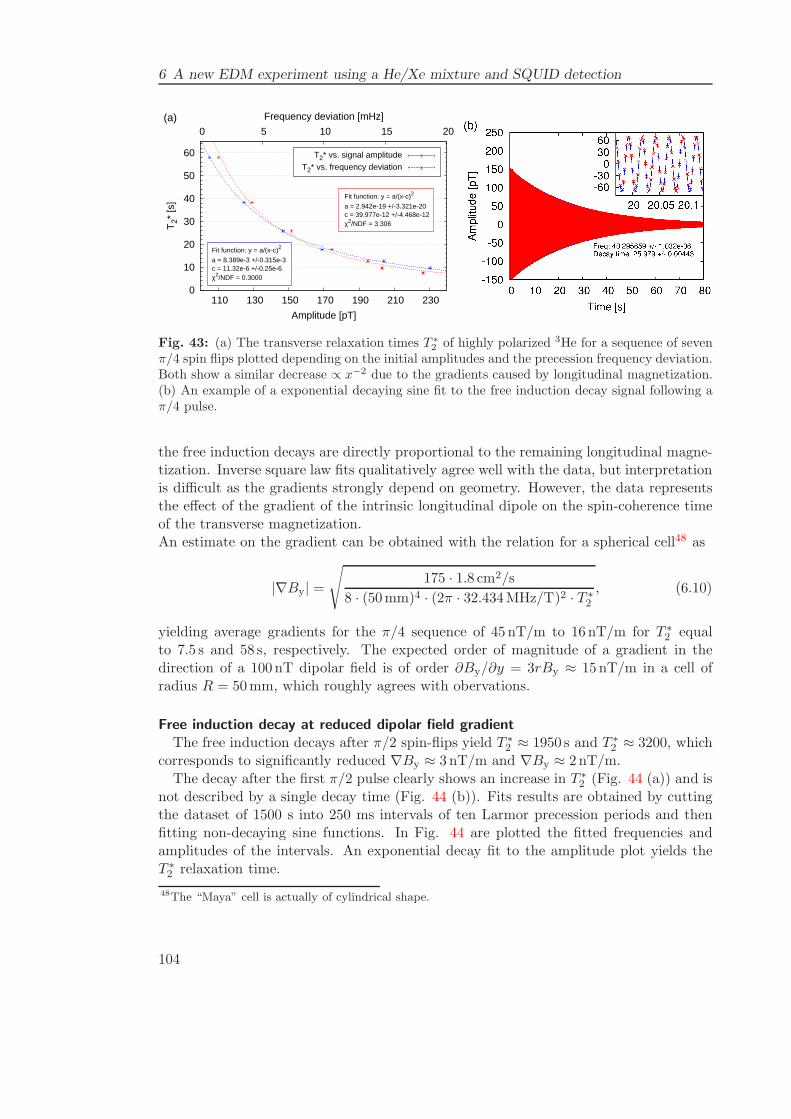
6 A new EDM experiment using a He/Xe mixture and SQUID detection
0
10
20
30
40
50
60
110 130 150 170 190 210 230
0 5 10 15 20
T2*
[s]
Amplitude [pT]
Frequency deviation [mHz](a)
T2* vs. signal amplitudeT2* vs. frequency deviation
Fit function: y = a/(x-c)2
a = 2.942e-19 +/-3.321e-20c = 39.977e-12 +/-4.468e-12χ2/NDF = 3.306
Fit function: y = a/(x-c)2
a = 8.389e-3 +/-0.315e-3c = 11.32e-6 +/-0.25e-6χ2/NDF = 0.3000
Fig. 43: (a) The transverse relaxation times T ∗
2 of highly polarized 3He for a sequence of sevenπ/4 spin flips plotted depending on the initial amplitudes and the precession frequency deviation.Both show a similar decrease ∝ x−2 due to the gradients caused by longitudinal magnetization.(b) An example of a exponential decaying sine fit to the free induction decay signal following aπ/4 pulse.
the free induction decays are directly proportional to the remaining longitudinal magne-tization. Inverse square law fits qualitatively agree well with the data, but interpretationis difficult as the gradients strongly depend on geometry. However, the data representsthe effect of the gradient of the intrinsic longitudinal dipole on the spin-coherence timeof the transverse magnetization.An estimate on the gradient can be obtained with the relation for a spherical cell48 as
|∇By| =√
175 · 1.8 cm2/s
8 · (50mm)4 · (2π · 32.434MHz/T)2 · T ∗2
, (6.10)
yielding average gradients for the π/4 sequence of 45 nT/m to 16 nT/m for T ∗2 equal
to 7.5 s and 58 s, respectively. The expected order of magnitude of a gradient in thedirection of a 100 nT dipolar field is of order ∂By/∂y = 3rBy ≈ 15 nT/m in a cell ofradius R = 50mm, which roughly agrees with obervations.
Free induction decay at reduced dipolar field gradientThe free induction decays after π/2 spin-flips yield T ∗
2 ≈ 1950 s and T ∗2 ≈ 3200, which
corresponds to significantly reduced ∇By ≈ 3 nT/m and ∇By ≈ 2 nT/m.The decay after the first π/2 pulse clearly shows an increase in T ∗
2 (Fig. 44 (a)) and isnot described by a single decay time (Fig. 44 (b)). Fits results are obtained by cuttingthe dataset of 1500 s into 250 ms intervals of ten Larmor precession periods and thenfitting non-decaying sine functions. In Fig. 44 are plotted the fitted frequencies andamplitudes of the intervals. An exponential decay fit to the amplitude plot yields theT ∗2 relaxation time.
48The “Maya” cell is actually of cylindrical shape.
104
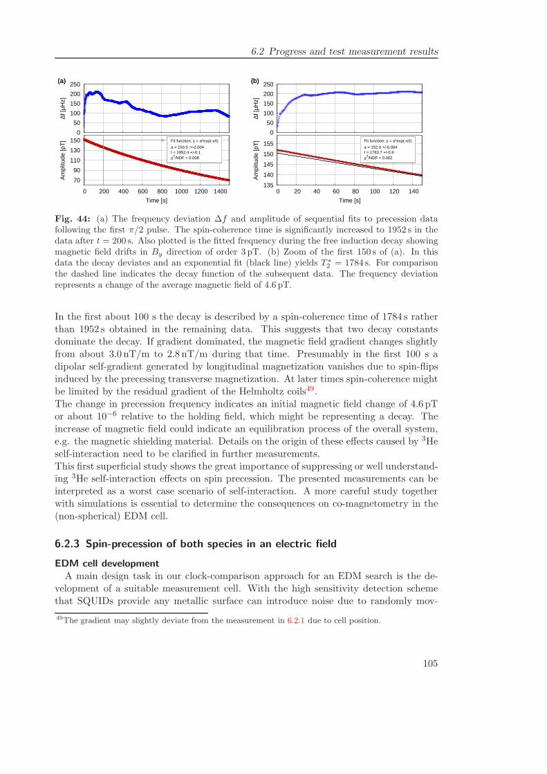
6.2 Progress and test measurement results
70
90
110
130
150
0 200 400 600 800 1000 1200 1400
Am
plitu
de [p
T]
Time [s]
(a)
Fit function: y = a*exp(-x/t)
a = 150.5 +/-0.004t = 1952.4 +/-0.1χ2/NDF = 0.008
0
50
100
150
200
250
∆f [µ
Hz]
(a)
Fit function: y = a*exp(-x/t)
a = 150.5 +/-0.004t = 1952.4 +/-0.1χ2/NDF = 0.008
135
140
145
150
155
0 20 40 60 80 100 120 140
Am
plitu
de [p
T]
Time [s]
(b)
Fit function: y = a*exp(-x/t)
a = 152.0 +/-0.004t = 1783.7 +/-0.9χ2/NDF = 0.002
0
50
100
150
200
250
∆f [µ
Hz]
(b)
Fit function: y = a*exp(-x/t)
a = 152.0 +/-0.004t = 1783.7 +/-0.9χ2/NDF = 0.002
Fig. 44: (a) The frequency deviation ∆f and amplitude of sequential fits to precession datafollowing the first π/2 pulse. The spin-coherence time is significantly increased to 1952 s in thedata after t = 200 s. Also plotted is the fitted frequency during the free induction decay showingmagnetic field drifts in By direction of order 3 pT. (b) Zoom of the first 150 s of (a). In thisdata the decay deviates and an exponential fit (black line) yields T ∗
2 = 1784 s. For comparisonthe dashed line indicates the decay function of the subsequent data. The frequency deviationrepresents a change of the average magnetic field of 4.6 pT.
In the first about 100 s the decay is described by a spin-coherence time of 1784 s ratherthan 1952 s obtained in the remaining data. This suggests that two decay constantsdominate the decay. If gradient dominated, the magnetic field gradient changes slightlyfrom about 3.0 nT/m to 2.8 nT/m during that time. Presumably in the first 100 s adipolar self-gradient generated by longitudinal magnetization vanishes due to spin-flipsinduced by the precessing transverse magnetization. At later times spin-coherence mightbe limited by the residual gradient of the Helmholtz coils49.The change in precession frequency indicates an initial magnetic field change of 4.6 pTor about 10−6 relative to the holding field, which might be representing a decay. Theincrease of magnetic field could indicate an equilibration process of the overall system,e.g. the magnetic shielding material. Details on the origin of these effects caused by 3Heself-interaction need to be clarified in further measurements.This first superficial study shows the great importance of suppressing or well understand-ing 3He self-interaction effects on spin precession. The presented measurements can beinterpreted as a worst case scenario of self-interaction. A more careful study togetherwith simulations is essential to determine the consequences on co-magnetometry in the(non-spherical) EDM cell.
6.2.3 Spin-precession of both species in an electric field
EDM cell developmentA main design task in our clock-comparison approach for an EDM search is the de-
velopment of a suitable measurement cell. With the high sensitivity detection schemethat SQUIDs provide any metallic surface can introduce noise due to randomly mov-
49The gradient may slightly deviate from the measurement in 6.2.1 due to cell position.
105
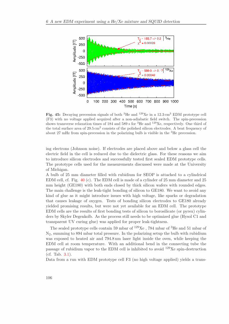
6 A new EDM experiment using a He/Xe mixture and SQUID detection
Fig. 45: Decaying precession signals of both 3He and 129Xe in a 12.3 cm3 EDM prototype cell(F3) with no voltage applied acquired after a non-adiabatic field switch. The spin-precessionshows transverse relaxation times of 184 and 589 s for 3He and 129Xe, respectively. One third ofthe total surface area of 29.5 cm2 consists of the polished silicon electrodes. A beat frequency ofabout 27 mHz from spin-precession in the polarizing bulb is visible in the 3He precession.
ing electrons (Johnson noise). If electrodes are placed above and below a glass cell theelectric field in the cell is reduced due to the dielectric glass. For these reasons we aimto introduce silicon electrodes and successfully tested first sealed EDM prototype cells.The prototype cells used for the measurements discussed were made at the Universityof Michigan.A bulb of 25 mm diameter filled with rubidium for SEOP is attached to a cylindricalEDM cell, cf. Fig. 40 (c). The EDM cell is made of a cylinder of 25 mm diameter and 25mm height (GE180) with both ends closed by thick silicon wafers with rounded edges.The main challenge is the leak-tight bonding of silicon to GE180. We want to avoid anykind of glue as it might introduce issues with high voltage, like sparks or degradationthat causes leakage of oxygen. Tests of bonding silicon electrodes to GE180 alreadyyielded promising results, but were not yet available for an EDM cell. The prototypeEDM cells are the results of first bonding tests of silicon to borosilicate (or pyrex) cylin-ders by Skyler Degenkolb. As the process still needs to be optimized glue (Hysol C1 andtransparent UV curing glue) was applied for proper leak-tightness.
The sealed prototype cells contain 59 mbar of 129Xe , 784 mbar of 3He and 51 mbar ofN2, summing to 894 mbar total pressure. In the polarizing setup the bulb with rubidiumwas exposed to heated air and 794.8 nm laser light inside the oven, while keeping theEDM cell at room temperature. With an additional bend in the connecting tube thepassage of rubidium vapor to the EDM cell is inhibited to avoid 129Xe spin-destruction(cf. Tab. 3.1).Data from a run with EDM prototype cell F3 (no high voltage applied) yields a trans-
106
6.2 Progress and test measurement results
verse spin-relaxation time of 3He and 129Xe of 184 s and 589 s, respectively (Fig. 45).Yet no spin-relaxation rates of 129Xe wall collisions with silicon have been reported.Without further studies we can set a limit on the relaxation rate from the observed T ∗
2 .
A limit on 129Xe wall relaxation on silicon surfacesIn our cell of glass and silicon surfaces the polished silicon electrodes amount to ASi ≈
9.8 cm2 at a total volume of the EDM cell and polarizing bulb of V ≈ 21.3 cm3. Toset a limit on wall relaxation on silicon, the total transverse spin relaxation rate can beassumed to be dominated by the wall relaxation on silicon, hence
Γtot = Γgrad + Γglass + ΓSi ≈ ΓSi, (6.11)
where relaxation due to diffusion in gradients Γgrad and wall relaxation on glass surfacesΓglass is neglected as both are assumed to be much smaller.Under this assumption and scaling to the silicon surface area, volume and 129Xe pressurea rough estimate on wall relaxation of a silicon surface of area A in a cell of volume Vand a 129Xe partial pressure of p is obtained as
ΓSi .1
589 s
21.3 cm3
9.8 cm2· 59mbar ≈ 2.2× 10⁻⁴A
V
1
p
cm · bars
. (6.12)
As can be seen in Fig. 45 the 3He signal dephases very quickly, on the order of tentimes faster than previously measured. The reason might not be depolarization on thepolished silicon surface but rather cracks and rough surfaces at the interfaces of theGE180 cylinder and the silicon electrodes. This needs to be solved by improved bondingand further analyzed in the future. However, the long relaxation times observed for129Xe strongly motivate further studies of silicon electrodes and bonding techniques toimprove on 3He relaxation.
Beat frequency in the EDM cellAnother feature in Fig. 45 can be attributed to the geometry currently used proto-
type cells with two chambers of similar volumes. The 3He precession exhibits a beatfrequency in the EDM cell originating from 3He precession in the polarizing bulb. Thebeat frequency is around 27 mHz and is not observable in 129Xe precession. Due tohigher pressure and gyromagnetic ratio the impact of precessing 3He is a factor of ≈ 40stronger than by 129Xe. The beat frequency translates into a magnetic field deviation inz-direction of 27mHz/(32.4Hz/µT) = 0.8 nT over the 65 mm between polarizing bulband EDM cell. Hence a (linear) gradient ∂Bz/∂z of order 13 nT/m can be estimated,which presumably originates from the magnetic field coils.
High voltage test runsPrototype EDM cells F3 and F4 were both tested with high voltage applied to the
electrodes using a high-voltage amplifier (Trek 610E). No sparks outside the cell were
107
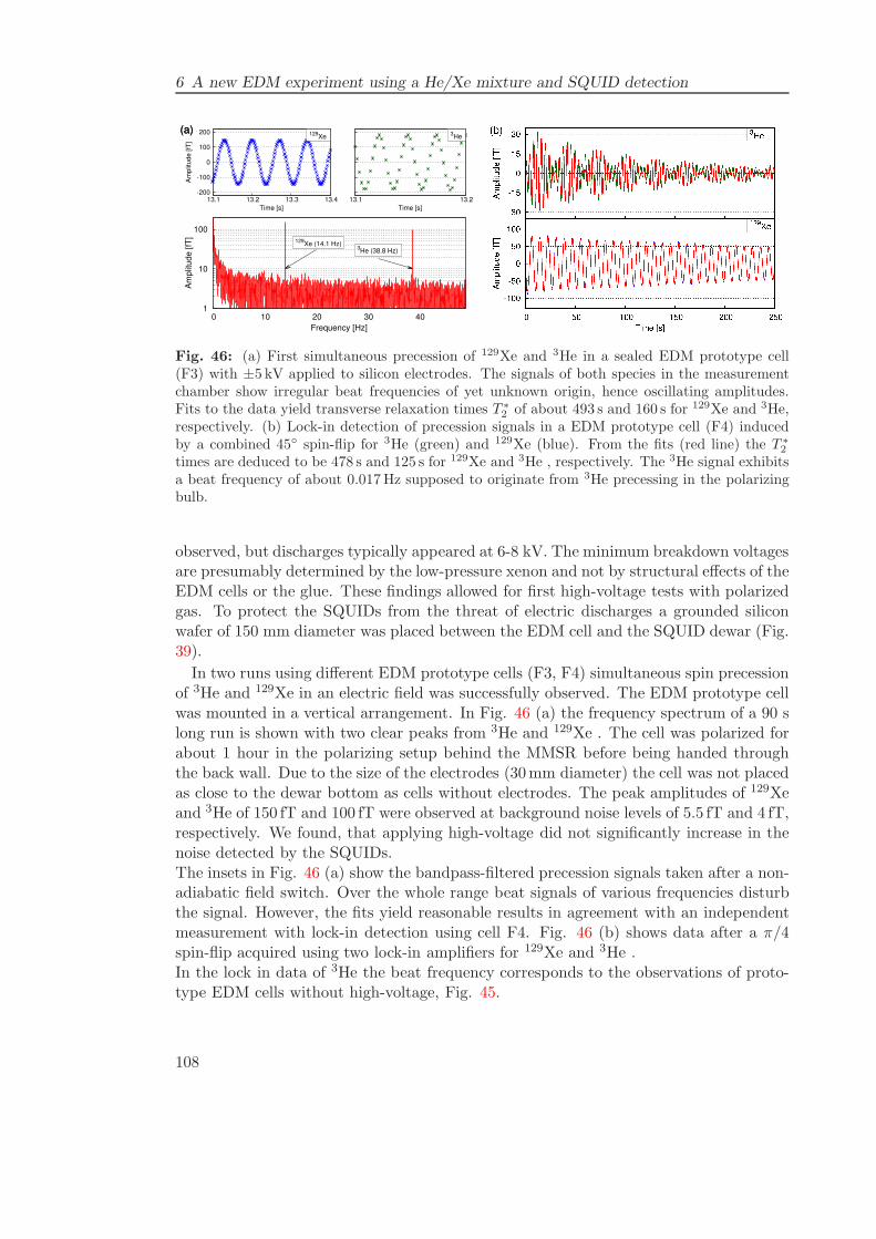
6 A new EDM experiment using a He/Xe mixture and SQUID detection
1
10
100
0 10 20 30 40
(a)
Am
plit
ude [fT
]
Frequency [Hz]
129Xe (14.1 Hz)
3He (38.8 Hz)
-200
-100
0
100
200
13.1 13.2 13.3 13.4
(a)
Am
plit
ude [fT
]
Time [s]
129Xe
13.1 13.2
Time [s]
3He
Fig. 46: (a) First simultaneous precession of 129Xe and 3He in a sealed EDM prototype cell(F3) with ±5 kV applied to silicon electrodes. The signals of both species in the measurementchamber show irregular beat frequencies of yet unknown origin, hence oscillating amplitudes.Fits to the data yield transverse relaxation times T ∗
2 of about 493 s and 160 s for 129Xe and 3He,respectively. (b) Lock-in detection of precession signals in a EDM prototype cell (F4) inducedby a combined 45 spin-flip for 3He (green) and 129Xe (blue). From the fits (red line) the T ∗
2
times are deduced to be 478 s and 125 s for 129Xe and 3He , respectively. The 3He signal exhibitsa beat frequency of about 0.017Hz supposed to originate from 3He precessing in the polarizingbulb.
observed, but discharges typically appeared at 6-8 kV. The minimum breakdown voltagesare presumably determined by the low-pressure xenon and not by structural effects of theEDM cells or the glue. These findings allowed for first high-voltage tests with polarizedgas. To protect the SQUIDs from the threat of electric discharges a grounded siliconwafer of 150 mm diameter was placed between the EDM cell and the SQUID dewar (Fig.39).
In two runs using different EDM prototype cells (F3, F4) simultaneous spin precessionof 3He and 129Xe in an electric field was successfully observed. The EDM prototype cellwas mounted in a vertical arrangement. In Fig. 46 (a) the frequency spectrum of a 90 slong run is shown with two clear peaks from 3He and 129Xe . The cell was polarized forabout 1 hour in the polarizing setup behind the MMSR before being handed throughthe back wall. Due to the size of the electrodes (30mm diameter) the cell was not placedas close to the dewar bottom as cells without electrodes. The peak amplitudes of 129Xeand 3He of 150 fT and 100 fT were observed at background noise levels of 5.5 fT and 4 fT,respectively. We found, that applying high-voltage did not significantly increase in thenoise detected by the SQUIDs.The insets in Fig. 46 (a) show the bandpass-filtered precession signals taken after a non-adiabatic field switch. Over the whole range beat signals of various frequencies disturbthe signal. However, the fits yield reasonable results in agreement with an independentmeasurement with lock-in detection using cell F4. Fig. 46 (b) shows data after a π/4spin-flip acquired using two lock-in amplifiers for 129Xe and 3He .In the lock in data of 3He the beat frequency corresponds to the observations of proto-type EDM cells without high-voltage, Fig. 45.
108
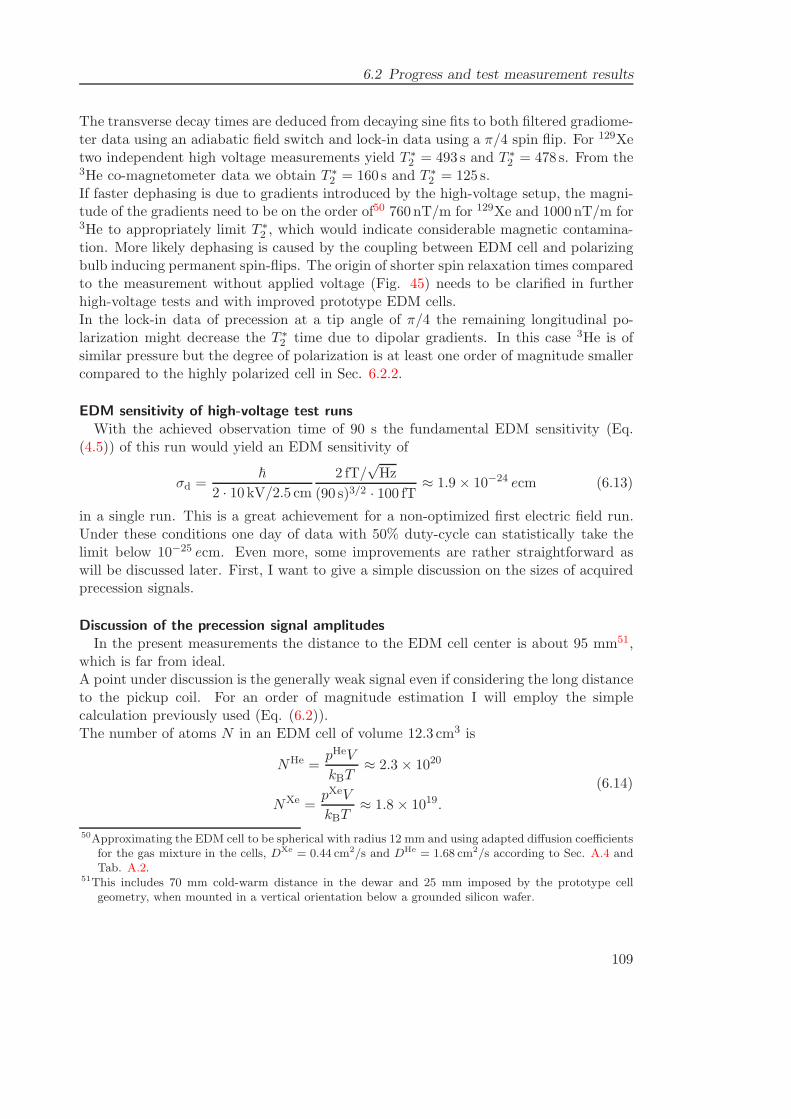
6.2 Progress and test measurement results
The transverse decay times are deduced from decaying sine fits to both filtered gradiome-ter data using an adiabatic field switch and lock-in data using a π/4 spin flip. For 129Xetwo independent high voltage measurements yield T ∗
2 = 493 s and T ∗2 = 478 s. From the
3He co-magnetometer data we obtain T ∗2 = 160 s and T ∗
2 = 125 s.If faster dephasing is due to gradients introduced by the high-voltage setup, the magni-tude of the gradients need to be on the order of50 760 nT/m for 129Xe and 1000 nT/m for3He to appropriately limit T ∗
2 , which would indicate considerable magnetic contamina-tion. More likely dephasing is caused by the coupling between EDM cell and polarizingbulb inducing permanent spin-flips. The origin of shorter spin relaxation times comparedto the measurement without applied voltage (Fig. 45) needs to be clarified in furtherhigh-voltage tests and with improved prototype EDM cells.In the lock-in data of precession at a tip angle of π/4 the remaining longitudinal po-larization might decrease the T ∗
2 time due to dipolar gradients. In this case 3He is ofsimilar pressure but the degree of polarization is at least one order of magnitude smallercompared to the highly polarized cell in Sec. 6.2.2.
EDM sensitivity of high-voltage test runsWith the achieved observation time of 90 s the fundamental EDM sensitivity (Eq.
(4.5)) of this run would yield an EDM sensitivity of
σd =~
2 · 10 kV/2.5 cm2 fT/
√Hz
(90 s)3/2 · 100 fT ≈ 1.9× 10⁻²⁴ ecm (6.13)
in a single run. This is a great achievement for a non-optimized first electric field run.Under these conditions one day of data with 50% duty-cycle can statistically take thelimit below 10−25 ecm. Even more, some improvements are rather straightforward aswill be discussed later. First, I want to give a simple discussion on the sizes of acquiredprecession signals.
Discussion of the precession signal amplitudesIn the present measurements the distance to the EDM cell center is about 95 mm51,
which is far from ideal.A point under discussion is the generally weak signal even if considering the long distanceto the pickup coil. For an order of magnitude estimation I will employ the simplecalculation previously used (Eq. (6.2)).The number of atoms N in an EDM cell of volume 12.3 cm3 is
NHe =pHeV
kBT≈ 2.3× 10²⁰
NXe =pXeV
kBT≈ 1.8 × 10¹⁹.
(6.14)
50Approximating the EDM cell to be spherical with radius 12 mm and using adapted diffusion coefficientsfor the gas mixture in the cells, DXe = 0.44 cm2/s and DHe = 1.68 cm2/s according to Sec. A.4 andTab. A.2.
51This includes 70 mm cold-warm distance in the dewar and 25 mm imposed by the prototype cellgeometry, when mounted in a vertical orientation below a grounded silicon wafer.
109
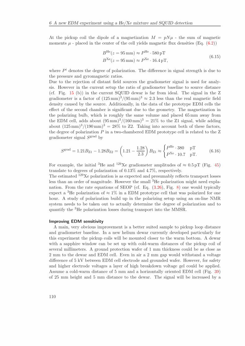
6 A new EDM experiment using a He/Xe mixture and SQUID detection
At the pickup coil the dipole of a magnetization M = pNµ - the sum of magneticmoments µ - placed in the center of the cell yields magnetic flux densities (Eq. (6.2))
BHe(z = 95mm) ≈ PHe · 580 pTBXe(z = 95mm) ≈ PXe · 16.4 pT,
(6.15)
where P i denotes the degree of polarization. The difference in signal strength is due tothe pressure and gyromagnetic ratios.Due to the rejection of distant field sources the gradiometer signal is used for analy-sis. However in the current setup the ratio of gradiometer baseline to source distance(cf. Fig. 15 (b)) in the current SQUID dewar is far from ideal. The signal in the Zgradiometer is a factor of (125mm)3/(95mm)3 ≈ 2.3 less than the real magnetic fielddensity caused by the source. Additionally, in the data of the prototype EDM cells theeffect of the second chamber is significant due to the geometry. The magnetization inthe polarizing bulb, which is roughly the same volume and placed 65mm away fromthe EDM cell, adds about (95mm)3/(160mm)3 = 21% to the Z1 signal, while addingabout (125mm)3/(190mm)3 = 28% to Z2. Taking into account both of these factors,the degree of polarization P in a two-chambered EDM prototype cell is related to the Zgradiometer signal Sgrad by
Sgrad = 1.21BZ1 − 1.28BZ2 =
(1.21 − 1.28
2.3
)BZ1 ≈
PHe · 380 pT
PXe · 10.7 pT.(6.16)
For example, the initial 3He and 129Xe gradiometer amplitudes of ≈ 0.5 pT (Fig. 45)translate to degrees of polarization of 0.13% and 4.7%, respectively.The estimated 129Xe polarization is as expected and presumably reflects transport lossesless than an order of magnitude. However the small 3He polarization might need expla-nation. From the rate equations of SEOP (cf. Eq. (3.26), Fig. 8) one would typicallyexpect a 3He polarization of ≈ 1% in a EDM prototype cell that was polarized for onehour. A study of polarization build up in the polarizing setup using an on-line NMRsystem needs to be taken out to actually determine the degree of polarization and toquantify the 3He polarization losses during transport into the MMSR.
Improving EDM sensitivityA main, very obvious improvement is a better suited sample to pickup loop distance
and gradiometer baseline. In a new helium dewar currently developed particularly forthis experiment the pickup coils will be mounted closer to the warm bottom. A dewarwith a sapphire window can be set up with cold-warm distances of the pickup coil ofseveral millimeters. A ground protection wafer of 1 mm thickness could be as close as2 mm to the dewar and EDM cell. Even in air a 2 mm gap would withstand a voltagedifference of 5 kV between EDM cell electrode and grounded wafer. However, for safetyand higher electrode voltages a layer of high breakdown voltage gel could be applied.Assume a cold-warm distance of 5 mm and a horizontally oriented EDM cell (Fig. 39)of 25 mm height and 5 mm distance to the dewar. The signal will be increased by a
110
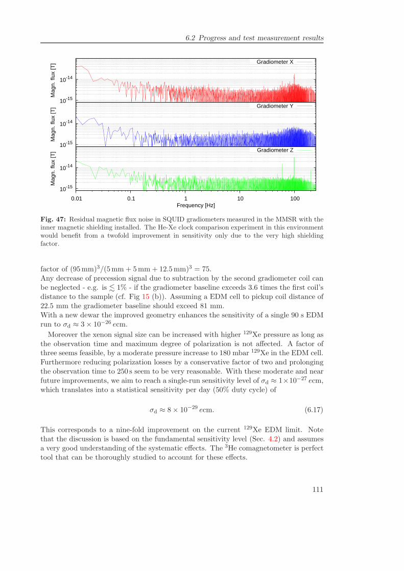
6.2 Progress and test measurement results
10-15
10-14
Mag
n. fl
ux [T
] Gradiometer X
10-15
10-14
Mag
n. fl
ux [T
] Gradiometer Y
10-15
10-14
0.01 0.1 1 10 100
Mag
n. fl
ux [T
]
Frequency [Hz]
Gradiometer Z
Fig. 47: Residual magnetic flux noise in SQUID gradiometers measured in the MMSR with theinner magnetic shielding installed. The He-Xe clock comparison experiment in this environmentwould benefit from a twofold improvement in sensitivity only due to the very high shieldingfactor.
factor of (95mm)3/(5mm + 5mm+ 12.5mm)3 = 75.Any decrease of precession signal due to subtraction by the second gradiometer coil canbe neglected - e.g. is . 1% - if the gradiometer baseline exceeds 3.6 times the first coil’sdistance to the sample (cf. Fig 15 (b)). Assuming a EDM cell to pickup coil distance of22.5 mm the gradiometer baseline should exceed 81 mm.With a new dewar the improved geometry enhances the sensitivity of a single 90 s EDMrun to σd ≈ 3× 10⁻²⁶ ecm.
Moreover the xenon signal size can be increased with higher 129Xe pressure as long asthe observation time and maximum degree of polarization is not affected. A factor ofthree seems feasible, by a moderate pressure increase to 180 mbar 129Xe in the EDM cell.Furthermore reducing polarization losses by a conservative factor of two and prolongingthe observation time to 250 s seem to be very reasonable. With these moderate and nearfuture improvements, we aim to reach a single-run sensitivity level of σd ≈ 1×10⁻²⁷ ecm,which translates into a statistical sensitivity per day (50% duty cycle) of
σd ≈ 8× 10⁻²⁹ ecm. (6.17)
This corresponds to a nine-fold improvement on the current 129Xe EDM limit. Notethat the discussion is based on the fundamental sensitivity level (Sec. 4.2) and assumesa very good understanding of the systematic effects. The 3He comagnetometer is perfecttool that can be thoroughly studied to account for these effects.
111
6 A new EDM experiment using a He/Xe mixture and SQUID detection
6.2.4 Potential of the magnetic shielding insert
Temporary installation of the inner shielding of the MMSR made possible a measurementof the noise floor in this highly shielded environment. The inner shield is a box of threelayers of µ-metal and when installed yields a shielding factor of ≈ 106 even at frequenciesdown to 100 mHz. The residual noise inside the inner shield measured with the X, Y,and Z gradiometers is shown in Fig. 47. Noise levels as low as 3 fT in the frequency rangeof interest are obtained . Assuming no other noise source, an EDM measurement wouldbenefit by a factor of two higher sensitivity simply due to the reduction of backgroundnoise.
6.3 Summary of the He/Xe EDM search
This work presents a first overview of the most significant data taken in two test runsfor the new He/Xe clock-comparison EDM experiment. The measurements show, thatspin-precession in a high electric field can be successfully detected in prototype EDMcells of cylindrical shape with bonded silicon electrodes. In these cells wall relaxationof 129Xe at the silicon surface was proven to be small enough to allow for several hun-dred seconds of observation time. The applied high voltage had no significant effect onspin-relaxation times and on the magnetic flux noise at the position of the SQUID cubein the current dewar. Under these conditions we showed that already now an EDM runcan be performed with a sensitivity on the order of ≈ 10−24 ecm for a single run of about100 s.Also a first study of self-interaction of polarized 3He in a highly polarized cell givesfirst hints on the significance of these effects. Remaining longitudinal magnetization canstrongly influence spin-precession in not perfectly spherical cells and introduce dipolarmagnetic field gradients that limit transverse spin coherence times. Detailed studies ofthese self-interaction effects need to be carried out both experimentally and in simula-tions. A good understanding helps finding the optimal experimental parameters and canprobably be used to account for this systematic in data analysis.The co-magnetometer approach offers fast progress applying well known methods withnow demonstrated improvements in EDM sensitivity well beyond current limits. Animproved SQUID detection system adapted to the demands of this EDM experimentand very slight improvements will establish a sound basis for a single run sensitivity of10−27 ecm.
112
7 Conclusion and outlook
Limits on EDMs of fundamental systems have profound implications on interactionsthat violate CP symmetry. The best absolute EDM limit to date was obtained fromthe diamagnetic atom 199Hg with the result dHg . 3.1 × 10⁻²⁹ ecm. These rather com-plex systems offer a wide range of coefficients of possible CP odd couplings that can beconfined. However, further significant improvements in sensitivity are extremely chal-lenging. Hence, in recent years the diamagnetic atom 129Xe attracted interest, as it offersenhanced sensitivity to semileptonic CP odd couplings. Moreover, adding a new limiton the EDM of 129Xe in the game improves current constraints on hadronic CP violatingsources from the 199Hg measurement by up to an order of magnitude.Based on the distinguished nature of 129Xe two complementary approaches to new excit-ing results were developed in the course of this thesis. With the demonstrated significantprogress towards new EDM experiments 129Xe can be used as a tool to study the differentsystematic effects as well as the particular physics reach. Both experiments potentiallyenhance the sensitivity on the current 129Xe EDM limit of ≈ 10−27 ecm by up to threeorders of magnitude. The signal-to-noise ratio is significantly increased in very low mag-netic holding fields by implementation of highly sensitive SQUID detection systems thatexhibit noise levels in the fT range even at frequencies down to several Hz.While the EDM experiment using a 3He co-magnetometer is based on an establishedmeasurement technique and offers a moderate improvement in sensitivity on a shorttime scale, the liquid 129Xe EDM experiment employs a novel method of time-varyingelectric fields requiring extensive R&D work, but featuring a high gain in sensitivity.Nevertheless, the systematic effects that commonly limit EDM sensitivities are utterlydifferent in both experiments. Each of these approaches offers a certain balance betweenthe time scale of expected results and the potential boost in EDM sensitivity. Combinedthey offer very powerful tools to cross-check results.
7.1 Progress towards a liquid 129Xe EDM experiment
Progress and the achievement of milestones towards a liquid xenon EDM search whichalso employs a novel measurement technique is presented in Sec. 5. With this approachwe intend to ultimately improve the sensitivity on the EDM of 129Xe by two to threeorders of magnitude to the 10−30 ecm level, with even higher statistical sensitivity.There are currently no efforts using liquid xenon in an EDM search other than ours52.However, due to the potential EDM sensitivity gain, the effort is worthwhile.
52An EDM experiment with liquid xenon based on a different approach than ours was proposed [130],but hasn’t reappeared since several years.
113
7 Conclusion and outlook
Using a liquid sample of hyper-polarized 129Xe offers a very high density, hence signalsize, in a very small volume of sub-millimeter dimensions. This both improves fieldhomogeneity, eases the application of high fields and makes simultaneous observationof many samples accessible. On the other hand large amounts of polarized 129Xe gasneed to be accumulated and liquefied, which is a rather difficult task experimentally.Particularly challenging is the implementation of a non-magnetic system to control thesample temperature (< 180K), while keeping close-by niobium pickup coils in the su-perconducting state (< 9K).In this thesis the practicability and performance of such a complex cryogen-free SQUIDsystem for highly sensitive detection of 129Xe spin-precession was demonstrated. Back-ground noise density levels of < 50 fT/
√Hz above frequencies of 50Hz were achieved. A
sensitivity of 144 fT/√Hz was reached in the cryogen-free EDM cryostat with the sample
stage at 161K and only a 1mm gap to the superconducting pickup coils. The samplestage was found to increase the noise by a factor of two to four, which is attributed toJohnson noise, but independent of sample temperature.The next milestone towards the realization of this experiment, a remotely operationalflow-through and accumulation setup, was demonstrated to produce large amounts ofhighly polarized 129Xe, that can be transfered to the EDM cryostat.An “EDM chip” prototype made of quartz, where three liquid samples of millimetersize can be enclosed by a pressure-actuated piston was developed. The plate of quartzis polished on all surfaces in contact with polarized gas and can be used to test spin-precession in separated volumes detected by three pickup coils below the individualsamples. The fabrication of cavities enclosing individual sub-millimeter liquid samples isnot straightforward, particularly under the requirements imposed. Neither etching normachining offers well suitable techniques. In the future the implementation of electrodessurrounding the individual droplets is the major challenging task and most probably acombination of milli- and micro-fabrication techniques will be necessary.A first evaluation of the measurement concept and estimation of systematic limitationswas taken out. The method offers on-line adjustment of individual electric field con-figurations of many simultaneous samples, hence providing a strong tool to study sys-tematics. New systematic effects that arise from time-varying electric fields (Tab. 5.1)mostly modulate the holding field on a . 10−6 level, which in contrast to the commonlyused static electric field approach does not limit the EDM sensitivity. The most severesystematic effect is generated by AC leakage currents in conjunction with misalignmentof the rotating electric field vector to the precessing polarization vector. This sensitivitylimiting systematic effect is expected to be manageable on a level below 10−30 ecm. Inpreparation of an EDM experiment an extensive study of systematic effects is essential.
In the context of this quick summary of progress and status, the liquid xenon EDMexperiment ultimately introducing time-varying electric fields is now set up for studiesof spin precession in hyper-polarized liquid 129Xe at very low magnetic fields (< 100µT)and subsequently determine the accessible sensitivity of the novel method.
114
7.2 Status of the clock-comparison 129Xe EDM search
7.2 Status of the clock-comparison 129Xe EDM search
Complementary to the liquid xenon EDM experiment, significant progress to a new EDMlimit and a first look into systematic effects of a newly started EDM search using gaseous129Xe and a 3He co-magnetometer is presented in Sec. 6. This alternative approach em-ploys enhanced measurement methods that are well established and is performed in aunique highly shielded environment, which was particularly developed for low energyprecision experiments.In this EDM experiment we employ the method of parallel magnetic and electric fieldsand look for a deviation in Larmor precession frequency, while subsequently reversingthe electric field direction. Most of the systematic effects can be accounted for by simul-taneous detection of 3He co-magnetometer precession, which yields the exact magneticfield that also 129Xe is subject to.First test measurements gave insight into systematic effects we need to take into account,like the self-interaction of a highly polarized 3He sample. The magnetization of the sam-ple in a non-spherical cell leads to several effects on spin-precession. We observed fastdephasing, off-resonant spin-flip pulses and precession frequency deviations due to thedipolar gradient, the strength of the intrinsic dipolar field and decay of the dipolar field,respectively. After a first study of these effects, the implications on the EDM experimenthave to be determined by future tests in EDM-type cells. With a good understanding ofthis self-interaction alongside simulations their effect on spin-precession can presumablybe accounted for in data analysis.A main achievement towards application of electric fields was the observation of trans-verse spin-precession in prototype EDM cells with silicon electrodes. Spin-coherencetimes on the order of 500 s and 180 s were determined for 129Xe and 3He, respectively.The long spin-coherence of 129Xe can be translated in an estimate on a limit of the wallrelaxation rate of xenon on silicon surfaces, not yet reported in the literature. For a cellof volume V , xenon pressure p and silicon surface area A the wall relaxation rate ΓSi
can be limited to ΓSi . 2.2× 10⁻⁴ AV
1pcm·bar
s . A fast depolarization of 3He is most likelydue to interfaces of the silicon wafers to the GE180 cylinder as the bonding procedureneeds to be optimized.The major success of simultaneous detection of spin-precession of 129Xe and 3He in EDMprototype cells with voltages of up to 10 kV applied to the silicon electrodes was an im-pressive demonstration of fast progress. The data of this single run with an appliedelectric field of 4 kV/cm and an observation time of only 90 s translate to an EDM sen-sitivity of 2× 10⁻²⁴ ecm. Thus, during this thesis we already demonstrated a sensitivityof
σd = 2.3× 10⁻²⁶ ecm√week
, (7.1)
which is only one order of magnitude away from the published state-of-the-art result.The main straightforward improvement for a competitive result, e.g. a SQUID dewarparticularly designed for the EDM experiment53 yielding a sensitivity gain of 75 is due
53In the currently used dewar for the first tests, the gradiometer baseline is far beyond the optimumand the distance of the cell to the SQUID sensor adds to about 95mm.
115
7 Conclusion and outlook
for availability within the next six months. With additionally increased 129Xe pressure(×3), optimizations in observation times (×2.5) and reduction of transport losses (×2)a total gain in sensitivity of roughly 1000 is expected.
Studies of systematic effects, e.g. self-interaction, and simulations are the most im-portant near future tasks. With the past progress and high signal-to-noise ratios dueto SQUID detection a new result on the EDM of 129Xe is expected within a year time.Further suggested improvements are deploying the experiment inside the inner magneticshielding box, which potentially reduces the background noise by a factor of two, andimplementation of the circulating gas concept to obtain statistics more easily.
116
A Appendix
A.1 Analytical expressions of nuclear moments
Assuming a heavy nucleus, the T ,P odd nucleon-nucleon interaction can be averagedover internal nucleons, thus simplifying to the effective Hamiltonian for a T ,P oddinteraction of an external (nonrelativistic) nucleon with spin σ and the internal corewith nuclear density ρA(r)
54
HTP =GF√2
ηa2mp
σ ·∇ρA(r), (A.1)
with Fermi’s coupling constant GF and the mass of the proton mp. The dimensionlessconstant
ηa =Z
Aηap +
N
Aηan (A.2)
characterizes the interaction strength of an external nucleon a with the core nucleonsp, n.The nuclear density and the nuclear potential U(r) are of similar shape, hence ρA(r) =ρA(0)U(0) U(r) is assumed and Eq. (A.1) can be rewritten in the form
HTP = ξσ ·∇U(r), ξ = ηG
2√2mp
ρA(0)
U(0)≈ −2× 10⁻²¹η cm. (A.3)
The problem is now reduced to solving the Schrodinger equation (H + U)ψ = Eψ of anucleon in a potential U = U + ξσ ·∇U(r). Therefore, the perturbed wavefunction is
ψ = (1 + ξσ ·∇U)ψ, with (H + U)ψ = Eψ. (A.4)
The electric dipole moment d, Schiff moment S and MQM M due to the excitationof the external nucleon interacting with the internal core with their characteristic valuesare
d = −eξ(q − Z
A
)tI ≈ 10−8ηa e fm
S = −eq10ξ
[(tI +
1
I + 1
)r2ext −
5
3tIr
2q
]≈ 10−7ηa e fm
3
M =e
mpξ(µ − q)(2I − 1)tI ≈ 10−8ηa e fm
(A.5)
54The nucleon-nucleon interaction reduces to a single term, since all other terms contain the spin of theinternal core nucleons, for which 〈σ〉 = 0.
117
A Appendix
where tI =
1, I = l + 1/2
− II+1 , I = l − 1/2.
(A.6)
In the above analytic results q is the charge and µ the magnetic moment of the nu-cleon, r2ext and r2q are the mean square radii of the external nucleon and the nuclearcharge, respectively and l is the orbital angular momentum of the external nucleon.While according to Eq. (A.5) in nuclei with an external proton there is a direct contribu-tion to the Schiff moment, nuclei with an unpaired neutron can’t directly contribute, asq = 0. Nevertheless, it has been shown [43, 44, 156] that paired protons virtually excitedby the field of the external neutron contribute on a similar level, effectively yielding anonvanishing Schiff moment with q ≈ O(0.1), cf. Eq. (A.5).
A.2 The relations of electron-nucleon coupling coefficients
The coupling strengths of the T ,P odd electron-nucleon interaction can be related inthe following way. An EDM contribution arises in third order perturbation theory andthen CSP can be related to the spin-dependent contribution CT via [30, 157]
(Z
ACSPp +
N
ACSPn
)I
I↔ 1.9 × 10³
1 + 0.3Z2α2A−2/3µ−1
⟨CTp
∑
p
σp + CTn
∑
n
σn
⟩, (A.7)
where α is the fine structure constant, µ the nuclear magnetic moment and the term 〈 〉denote averaging over the nuclear state. With the help of Eq. (A.7) an EDM measure-ment of a diamagnetic atom can also set a competitive limit on CSP.
The weakest contribution from pseudoscalar-scalar terms CPS can also be related toCT by comparing the results of the matrix elements, thus obtaining [30, 157]
CPS ↔ 4.6× 10³A1/3
ZCT. (A.8)
Due to the above relations EDM searches using diamagnetic atoms can set limits on allthree spin-dependent and spin-independent T ,P odd interactions of electrons with thenuclei, cf. Tab. 2.3.
A.3 A limit on the electon EDM from diamagnetic atoms
An electron EDM induces an atomic EDM of diamagnetic atoms due to polarization ofthe closed electron shell along the nuclear spin by the hyperfine interaction. In thirdorder perturbation theory [30, 31]
HTPhf = eµ
r ×α
r3, with α =
(0 σ
σ 0
)(A.9)
118
A.4 Diffusion in multi-component gas mixtures
and the nuclear magnetic moment µ = eµ2mp
I
I .The second, more important contribution emerges from a direct interaction of the elec-tron EDM with the magnetic moment of the nucleus µ:
HTPµ = −ideγ ·B = −ideγ ·∇×
(∇
1
r× µ
)with γ =
(0 σ
−σ 0
)(A.10)
The total matrix element mixing s1/2 and p1/2 states in diamagnetic atoms is given in[30] as
〈s1/2|HTPµ +HTP
hf |p1/2〉 = −de7
3
eµ
mp
Z2α(R − 1)
a3(νsνp)3/22j · II
, (A.11)
where a is the Bohr radius and the relativistic enhancement factor
R =4
Γ2(2γ + 1)
(a
2ZR0
)2−2γ
. (A.12)
Here, γ =√(j + 1/2)2 − Z2α2 and R0 is the nuclear radius.
With this result the following relation can be established between the electron EDM deand the tensor interaction of electrons and nucleons (cf. Eq. (2.15))
deI
I↔ 3
7
GFmpe√2παµ
R
R− 1
⟨CTp
∑
p
σp + CTn
∑
n
σn
⟩(A.13)
With the help of this relation the numeric calculations of CT can be used to set a limiton the electron EDM with measurements on diamagnetic atoms.
A.4 Diffusion in multi-component gas mixtures
In gas mixtures the diffusion coefficients of helium and xenon are altered according to
1
DHe=
pHe
DHeHe+
pXe
DHeXe+
pN2
DHeN2(A.14)
and1
DXe=
pXe
DXeXe+
pHe
DXeHe+
pN2
DXeN2, (A.15)
where Dii is the coefficient of self-diffusion and Dij is the coefficient of diffusion of i inj. Appropriate binary diffusion coefficients are given in Tab. A.2.
119
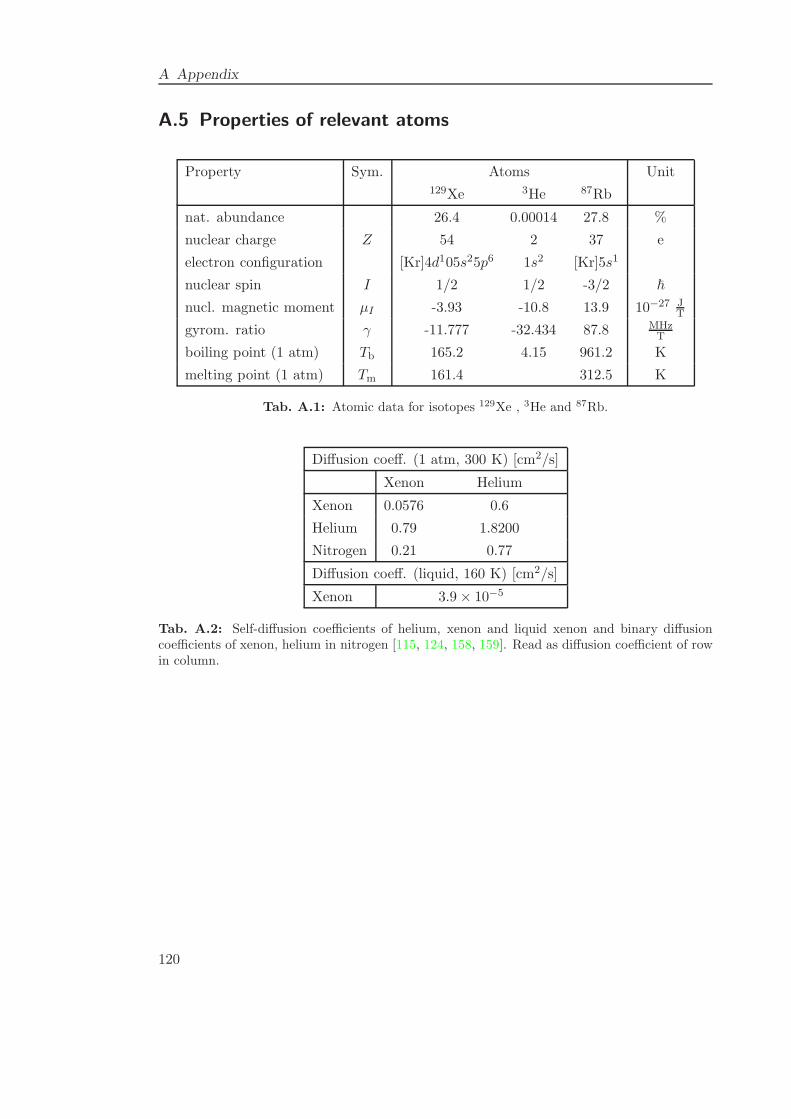
A Appendix
A.5 Properties of relevant atoms
Property Sym. Atoms Unit129Xe 3He 87Rb
nat. abundance 26.4 0.00014 27.8 %
nuclear charge Z 54 2 37 e
electron configuration [Kr]4d105s25p6 1s2 [Kr]5s1
nuclear spin I 1/2 1/2 -3/2 ~
nucl. magnetic moment µI -3.93 -10.8 13.9 10−27 JT
gyrom. ratio γ -11.777 -32.434 87.8 MHzT
boiling point (1 atm) Tb 165.2 4.15 961.2 K
melting point (1 atm) Tm 161.4 312.5 K
Tab. A.1: Atomic data for isotopes 129Xe , 3He and 87Rb.
Diffusion coeff. (1 atm, 300 K) [cm2/s]
Xenon Helium
Xenon 0.0576 0.6
Helium 0.79 1.8200
Nitrogen 0.21 0.77
Diffusion coeff. (liquid, 160 K) [cm2/s]
Xenon 3.9× 10⁻⁵
Tab. A.2: Self-diffusion coefficients of helium, xenon and liquid xenon and binary diffusioncoefficients of xenon, helium in nitrogen [115, 124, 158, 159]. Read as diffusion coefficient of rowin column.
120
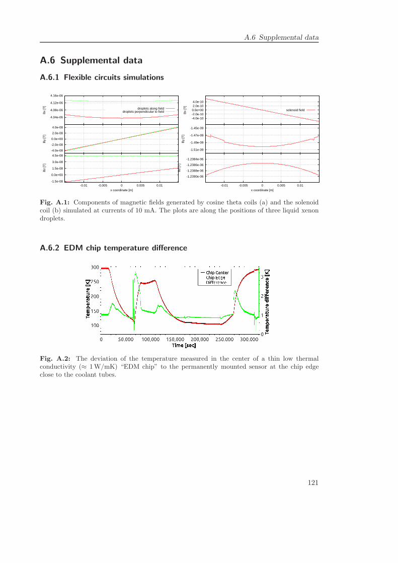
A.6 Supplemental data
A.6 Supplemental data
A.6.1 Flexible circuits simulations
4.04e-06
4.08e-06
4.12e-06
4.16e-06
Bx
[T]
droplets along fielddroplets perpendicular to field
-4.0e-08
-2.0e-08
0.0e+00
2.0e-08
4.0e-08
By
[T]
-1.5e-08
0.0e+00
1.5e-08
3.0e-08
4.5e-08
-0.01 -0.005 0 0.005 0.01
Bz
[T]
x coordinate [m]
-4.0e-10-2.0e-100.0e+002.0e-104.0e-10
Bx
[T]
solenoid field
-1.51e-09
-1.49e-09
-1.47e-09
-1.45e-09
By
[T]
-1.2390e-06
-1.2388e-06
-1.2386e-06
-1.2384e-06
-0.01 -0.005 0 0.005 0.01
Bz
[T]
x coordinate [m]
Fig. A.1: Components of magnetic fields generated by cosine theta coils (a) and the solenoidcoil (b) simulated at currents of 10 mA. The plots are along the positions of three liquid xenondroplets.
A.6.2 EDM chip temperature difference
Fig. A.2: The deviation of the temperature measured in the center of a thin low thermalconductivity (≈ 1W/mK) “EDM chip” to the permanently mounted sensor at the chip edgeclose to the coolant tubes.
121
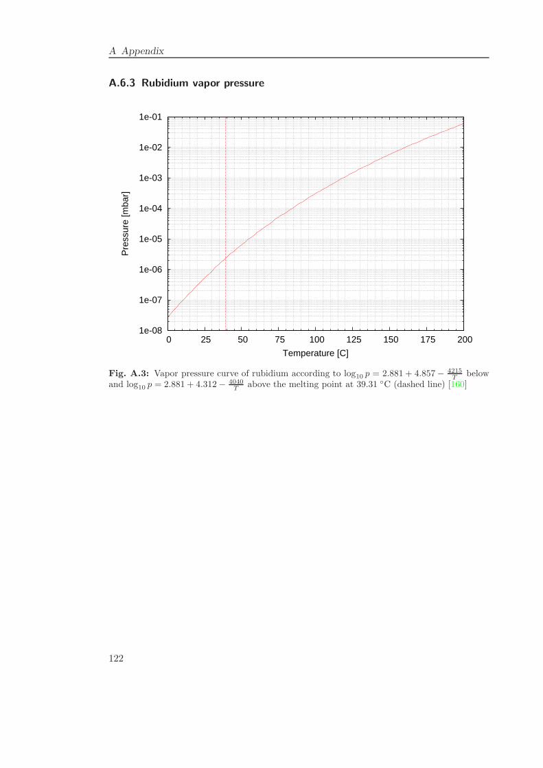
A Appendix
A.6.3 Rubidium vapor pressure
1e-08
1e-07
1e-06
1e-05
1e-04
1e-03
1e-02
1e-01
0 25 50 75 100 125 150 175 200
Pre
ssur
e [m
bar]
Temperature [C]
Fig. A.3: Vapor pressure curve of rubidium according to log10 p = 2.881 + 4.857− 4215T below
and log10 p = 2.881 + 4.312− 4040T above the melting point at 39.31 C (dashed line) [160]
122
List of Figures
1 Transformation of polar and axial vectors . . . . . . . . . . . . . . . . . . 62 EDM contributions in different systems . . . . . . . . . . . . . . . . . . . 73 Evolution of published EDM limits . . . . . . . . . . . . . . . . . . . . . . 134 Loop diagrams generating EDMs in the SM and in SUSY models . . . . . 145 Constrains on MSSM phases from EDM limits . . . . . . . . . . . . . . . 16
6 Level splittings and optical pumping scheme of Rb . . . . . . . . . . . . . 227 Spin-exchange collisions . . . . . . . . . . . . . . . . . . . . . . . . . . . . 308 Buildup of 129Xe and 3He polarization according to the rate-model . . . . 329 Dependence of wall-relaxation on magnetic field . . . . . . . . . . . . . . . 3510 Transverse spin relaxation due to diffusion in magnetic field gradients . . 3611 Longitudinal relaxation in solid 129Xe in high and low magnetic fields . . 3912 Transverse spin relaxation in liquid 129Xe due magnetic field graidents . . 4113 SQUID operation principle . . . . . . . . . . . . . . . . . . . . . . . . . . 4414 SQUID voltage modulation and FLL circuit . . . . . . . . . . . . . . . . . 4515 Superconducting flux transformer and gradiometer response . . . . . . . . 46
16 Experimental setup of the He-Xe maser . . . . . . . . . . . . . . . . . . . 50
17 Overview of the liquid xenon setup . . . . . . . . . . . . . . . . . . . . . . 5618 Measurement principle of the liquid xenon EDM experiment . . . . . . . . 5819 Simultanous experiments with different field configurations . . . . . . . . 5920 Electric field misalignment and example arrangement with dimensions . . 6321 Dominating systematic due to AC leakage currents of opposite electrodes 6422 Scheme of the cooling system for the “EDM chip” . . . . . . . . . . . . . 7123 The sample glass tube and the superconducting pickup coils . . . . . . . . 7224 SQUID cryostat cooldown and temperature stability . . . . . . . . . . . . 7525 Magnetic flux noise spectra in the SQUID cryostat . . . . . . . . . . . . . 7626 Dependence of the magnetic flux noise on sample temperature . . . . . . . 7727 Transition to the normal state of a superconducting ring . . . . . . . . . . 7828 SQUID calibration and a picture of the liquid xenon setup pickup coils . . 8129 Scheme of the SEOP setup of the liquid xenon EDM . . . . . . . . . . . . 8230 Polarizing cell and non-magnetic high vacuum valves . . . . . . . . . . . . 8331 Exponential buildup of 129Xe polarization in the SEOP setup . . . . . . . 8432 On-line NMR of 129Xe and calibration with . . . . . . . . . . . . . . . . . 8533 The cold trap setup for accumulation of polarized 129Xe . . . . . . . . . . 8634 NMR probe system and evaluation of accumulation losses . . . . . . . . . 8735 Effect of degaussing of the magnetic shields on magnetic flux density . . . 88
123
List of Figures
36 Magnetic fields generated by flexible printed circuit boards . . . . . . . . 8937 The “EDM chip” prototype and the pressure actuator . . . . . . . . . . . 91
38 Buildup of 3He polarization normalized to 129Xe . . . . . . . . . . . . . . 9639 Overview of the He/Xe clock comparison setup . . . . . . . . . . . . . . . 9840 Test setup in the magnetically shielded room and EDM prototype cell . . 9941 First spin precession signal of 129Xe . . . . . . . . . . . . . . . . . . . . . 10142 Pulse sequence applied to highly polarized 3He cell . . . . . . . . . . . . . 10243 Analysis of the π/4 pulse sequence . . . . . . . . . . . . . . . . . . . . . . 10444 Analysis of interaction of longitudinal polarization on precessing 3He spins 10545 Simultaneous precession of 3He and 129Xe in an EDM prototype cell with-
out electric field . . . . . . . . . . . . . . . . . . . . . . . . . . . . . . . . . 10646 Simultaneous precession of 3He and 129Xe in an EDM prototype cell with
appied electric field . . . . . . . . . . . . . . . . . . . . . . . . . . . . . . . 10847 SQUID noise spectra inside the inner magnetic shielding . . . . . . . . . . 111
A.1 Flexible circuit magnetic field simulations . . . . . . . . . . . . . . . . . . 121A.2 Temperature deviation on the “EDM chip” . . . . . . . . . . . . . . . . . 121A.3 Vapor pressure of rubidium . . . . . . . . . . . . . . . . . . . . . . . . . . 122
124
List of Tables
2.1 Nuclear CP violating moments induced by the nucleon-nucleon interaction 92.2 Atom EDMs induced by the nuclear Schiff moments . . . . . . . . . . . . 102.3 Atom EDMs induced by the electron-nucleon interaction . . . . . . . . . . 112.4 Enhancement factors for the electron EDM . . . . . . . . . . . . . . . . . 122.5 Sensitivities of different systems to CP violating mechanisms . . . . . . . 162.6 Current EDM limits and predictions . . . . . . . . . . . . . . . . . . . . . 182.7 Comparison of sensitivities of 129Xe and 199Hg to CP odd atomic parameters 19
3.1 Spin-exchange and spin-destruction rates of 129Xe and 3He . . . . . . . . 273.2 Molecular spin-exchange rates for 129Xe . . . . . . . . . . . . . . . . . . . 30
5.1 Summary of systematic effects in the liquid xenon EDM experiment . . . 675.2 Simulated magnetic field quality . . . . . . . . . . . . . . . . . . . . . . . 90
A.1 Atomic data for isotopes 129Xe , 3He and 87Rb. . . . . . . . . . . . . . . . 120A.2 Binary diffusion coefficients of helium and xenon . . . . . . . . . . . . . . 120
125

Bibliography
[1] Georges Aad et al. “Observation of a new particle in the search for the StandardModel Higgs boson with the ATLAS detector at the LHC”. Phys.Lett. B716(2012), pp. 1–29.doi: 10.1016/j.physletb.2012.08.020. arXiv: 1207.7214 [hep-ex].
[2] Serguei Chatrchyan et al. “Observation of a new boson at a mass of 125 GeVwith the CMS experiment at the LHC”. Phys.Lett. B716 (2012), pp. 30–61.doi: 10.1016/j.physletb.2012.08.021. arXiv: 1207.7235 [hep-ex].
[3] G. Steigman. “Observational Tests of Antimatter Cosmologies”. Annual Reviewof Astronomy and Astrophysics 14 (1976), pp. 339–372.doi: 10.1146/annurev.aa.14.090176.002011.
[4] F. W. Stecker. “On the nature of the baryon asymmetry”. Nuclear Physics B 252(1985), pp. 25–36.doi: 10.1016/0550-3213(85)90423-7.
[5] A. G. Cohen, A. De Rujula, and S. L. Glashow. “A Matter-Antimatter Universe?”The Astrophysical Journal 495 (1998), p. 539.doi: 10.1086/305328. arXiv: astro-ph/9707087 [astro-ph].
[6] C. L. Bennett et al. “First year Wilkinson Microwave Anisotropy Probe (WMAP)observations: Preliminary maps and basic results”. Astrophys.J.Suppl. 148 (2003),p. 1.doi: 10.1086/377253. arXiv: astro-ph/0302207 [astro-ph].
[7] P.A.R. Ade et al. “Planck 2013 results. XVI. Cosmological parameters”. As-tron.Astrophys. (2014).doi: 10.1051/0004-6361/201321591. arXiv: 1303.5076 [astro-ph.CO].
[8] Lawrence M. Krauss and Peter J. Kernan. “Big Bang Nucleosynthesis constraintsand light element abundance estimates”. Physics Letters B 347 (1995), pp. 347–353.doi: 10.1016/0370-2693(95)00082-V.
[9] G. Borner. The Early Universe: Facts and Fiction. 4th ed. Astronomy and As-trophysics Library. Springer, 2003.
[10] James M. Cline. Baryogenesis. arXiv: hep-ph/0609145 [hep-ph].
[11] Laurent Canetti, Marco Drewes, and Mikhail Shaposhnikov. “Matter and anti-matter in the universe”. New Journal of Physics 14 (2012), p. 095012.
127
Bibliography
[12] A. D. Sakharov. “Violation of CP Invariance, C Asymmetry, and Baryon Asym-metry of the Universe”. Pisma Zh.Eksp.Teor.Fiz. 5 (1967), pp. 32–35.doi: 10.1070/PU1991v034n05ABEH002497.
[13] Mark Trodden. “Electroweak baryogenesis”. Rev.Mod.Phys. 71 (1999), pp. 1463–1500.doi: 10.1103/RevModPhys.71.1463. arXiv: hep-ph/9803479 [hep-ph].
[14] Michael Dine and Alexander Kusenko. “The Origin of the matter - antimatterasymmetry”. Rev.Mod.Phys. 76 (2004), p. 1.doi: 10.1103/RevModPhys.76.1. arXiv: hep-ph/0303065 [hep-ph].
[15] Sacha Davidson, Enrico Nardi, and Yosef Nir. “Leptogenesis”. Physics Reports466 (2008), pp. 105–177.doi: 10.1016/j.physrep.2008.06.002.
[16] G. ’t Hooft. “Symmetry Breaking through Bell-Jackiw Anomalies”. Phys. Rev.Lett. 37 (1976), pp. 8–11.doi: 10.1103/PhysRevLett.37.8.
[17] V. A. Kuzmin, V. A. Rubakov, and M. E. Shaposhnikov. “On anomalous elec-troweak baryon-number non-conservation in the early universe”. Physics LettersB 155 (1985), pp. 36–42.doi: 10.1016/0370-2693(85)91028-7.
[18] V. Gribov and B. Pontecorvo. “Neutrino astronomy and lepton charge”. PhysicsLetters B 28 (1969), pp. 493–496.doi: 10.1016/0370-2693(69)90525-5.
[19] K. S. Hirata et al. “Observation of a small atmospheric vµ/ve ratio in Kamiokande”.Physics Letters B 280 (1992), pp. 146–152.doi: 10.1016/0370-2693(92)90788-6.
[20] Q. R. Ahmad et al. “Direct Evidence for Neutrino Flavor Transformation fromNeutral-Current Interactions in the Sudbury Neutrino Observatory”. Phys. Rev.Lett. 89 (2002), p. 011301.doi: 10.1103/PhysRevLett.89.011301.
[21] C. S. Wu et al. “Experimental Test of Parity Conservation in Beta Decay”. Phys.Rev. 105 (1957), pp. 1413–1415.doi: 10.1103/PhysRev.105.1413.
[22] T. D. Lee and C. N. Yang. “Question of Parity Conservation in Weak Interac-tions”. Phys. Rev. 104 (1956), pp. 254–258.doi: 10.1103/PhysRev.104.254.
[23] L. Landau. “On the conservation laws for weak interactions”. Nuclear Physics 3(1957), pp. 127–131.doi: 10.1016/0029-5582(57)90061-5.
128
Bibliography
[24] J. H. Christenson et al. “Evidence for the 2π Decay of the K02 Meson”. Phys.
Rev. Lett. 13 (1964), pp. 138–140.doi: 10.1103/PhysRevLett.13.138.
[25] A. Abashian et al. “Measurement of the CP Violation Parameter sin2ϕ1 in B0d
Meson Decays”. Phys. Rev. Lett. 86 (2001), pp. 2509–2514.doi: 10.1103/PhysRevLett.86.2509.
[26] B. Aubert et al. “Measurement of CP -Violating Asymmetries in B0 Decays toCP Eigenstates”. Phys. Rev. Lett. 86 (2001), pp. 2515–2522.doi: 10.1103/PhysRevLett.86.2515.
[27] Nicola Cabibbo. “Unitary Symmetry and Leptonic Decays”. Phys. Rev. Lett. 10(1963), pp. 531–533.doi: 10.1103/PhysRevLett.10.531.
[28] Makoto Kobayashi and Toshihide Maskawa. “CP-Violation in the RenormalizableTheory of Weak Interaction”. Progress of Theoretical Physics 49 (1973), pp. 652–657.doi: 10.1143/PTP.49.652. eprint: http://ptp.oxfordjournals.org/content/49/2/652.full.pdf+html.
[29] O. W. Greenberg. “CPT Violation Implies Violation of Lorentz Invariance”. Phys.Rev. Lett. 89 (2002), p. 231602.doi: 10.1103/PhysRevLett.89.231602.
[30] Iosif B. Khriplovich and Steve K. Lamoreaux. CP Violation Without Strangeness.Electric Dipole Moments of Particles, Atoms, and Molecules. Springer Berlin Hei-delberg, 1997.doi: 10.1007/978-3-642-60838-4.
[31] J.S.M. Ginges and V.V. Flambaum. “Violations of fundamental symmetries inatoms and tests of unification theories of elementary particles”. Physics Reports397 (2004), p. 63.doi: 10.1016/j.physrep.2004.03.005.
[32] Maxim Pospelov and Adam Ritz. “Electric dipole moments as probes of newphysics”. Annals Phys. 318 (2005), pp. 119–169.doi: 10.1016/j.aop.2005.04.002. arXiv: nucl-th/0304048 [hep-ph].
[33] Jonathan Engel, Michael J. Ramsey-Musolf, and U. van Kolck. “Electric DipoleMoments of Nucleons, Nuclei, and Atoms: The Standard Model and Beyond”.Prog.Part.Nucl.Phys. 71 (2013), pp. 21–74.doi: 10.1016/j.ppnp.2013.03.003. arXiv: 1303.2371 [nucl-th].
[34] L. I. Schiff. “Measurability of Nuclear Electric Dipole Moments”. Phys. Rev. 132(1963), pp. 2194–2200.doi: 10.1103/PhysRev.132.2194.
[35] P. G. H. Sandars. “The electric dipole moment of an atom”. Physics Letters 14(1965), pp. 194–196.doi: 10.1016/0031-9163(65)90583-4.
129
Bibliography
[36] P.G.H. Sandars. “Enhancement factor for the electric dipole moment of the va-lence electron in an alkali atom”. Physics Letters 22 (1966), pp. 290–291.doi: 10.1016/0031-9163(66)90618-4.
[37] V. Spevak, N. Auerbach, and V. V. Flambaum. “Enhanced T-odd, P-odd elec-tromagnetic moments in reflection asymmetric nuclei”. Phys. Rev. C 56 (1997),pp. 1357–1369.doi: 10.1103/PhysRevC.56.1357.
[38] J. Engel, J. L. Friar, and A. C. Hayes. “Nuclear octupole correlations and the en-hancement of atomic time-reversal violation”. Phys. Rev. C 61 (2000), p. 035502.doi: 10.1103/PhysRevC.61.035502.
[39] L. P. Gaffney et al. “Studies of pear-shaped nuclei using accelerated radioactivebeams”. Nature 497 (2013), pp. 199–204.doi: 10.1038/nature12073.
[40] V. V. Flambaum and V. G. Zelevinsky. “Enhancement of nuclear Schiff momentsand time-reversal violation in atoms due to soft nuclear octupole vibrations”.Phys. Rev. C 68 (2003), p. 035502.doi: 10.1103/PhysRevC.68.035502.
[41] J. R. Guest et al. “Laser Trapping of Ra225 and Ra226 with Repumping by Room-Temperature Blackbody Radiation”. Phys. Rev. Lett. 98 (2007), p. 093001.doi: 10.1103/PhysRevLett.98.093001.
[42] E. R. Tardiff et al. “Polarization and relaxation rates of radon”. Phys. Rev. C 77(2008), p. 052501.doi: 10.1103/PhysRevC.77.052501.
[43] V.V. Flambaum, I.B. Khriplovich, and O.P. Sushkov. “Limit on the constantof T-nonconserving nucleon-nucleon interaction”. Physics Letters B 162 (1985),pp. 213–216.doi: 10.1016/0370-2693(85)90908-6.
[44] V. V. Flambaum, I. B. Khriplovich, and O. P. Sushkov. “On the P and T Non-conserving Nuclear Moments”. Nucl.Phys. A449 (1986), p. 750.doi: 10.1016/0375-9474(86)90331-3.
[45] O. P. Sushkov, V. V. Flambaum, and I. B. Khriplovich. “Possibility of investi-gating P- and T-odd nuclear forces in atomic and molecular experiments”. Sov.Phys. JETP 60 (1984), p. 873.doi: 10.1103/PhysRevA.87.012102.
[46] V.A. Dzuba et al. “Electric dipole moments of Hg, Xe, Rn, Ra, Pu, and TlFinduced by the nuclear Schiff moment and limits on time reversal violating inter-actions”. Phys.Rev. A66 (2002), p. 012111.doi: 10.1103/PhysRevA.66.012111. arXiv: hep-ph/0203202 [hep-ph].
[47] I. B. Khriplovich. “A bound on the proton electric dipole moment derived fromatomic experiments”. Sov. Phys. JETP 44 (1976), p. 25.
130
Bibliography
[48] Martin Jung and Antonio Pich. “Electric Dipole Moments in Two-Higgs-DoubletModels” (2013). arXiv: 1308.6283 [hep-ph].
[49] Matthias Dall and Adam Ritz. “CP-violation and electric dipole moments”. En-glish. Hyperfine Interactions 214 (2013), pp. 87–95.doi: 10.1007/s10751-013-0801-1.
[50] I.I. Bigi and N.G. Uraltsev. “Induced multi-gluon couplings and the neutronelectric dipole moment”. Nuclear Physics B 353 (1991), pp. 321–336.doi: 10.1016/0550-3213(91)90339-Y.
[51] John Paul Archambault, Andrzej Czarnecki, andMaxim Pospelov. “Electric dipolemoments of leptons in the presence of Majorana neutrinos”. Phys. Rev. D 70(2004), p. 073006.doi: 10.1103/PhysRevD.70.073006.
[52] C. Jarlskog. “Commutator of the Quark Mass Matrices in the Standard Elec-troweak Model and a Measure of Maximal CP Nonconservation”. Phys. Rev.Lett. 55 (1985), pp. 1039–1042.doi: 10.1103/PhysRevLett.55.1039.
[53] R.J. Crewther et al. “Chiral estimate of the electric dipole moment of the neutronin quantum chromodynamics”. Physics Letters B 88 (1979), pp. 123–127.doi: 10.1016/0370-2693(79)90128-X.
[54] Maxim Pospelov and Adam Ritz. “Theta-Induced Electric Dipole Moment of theNeutron via QCD Sum Rules”. Phys. Rev. Lett. 83 (1999), pp. 2526–2529.doi: 10.1103/PhysRevLett.83.2526.
[55] C. A. Baker et al. “Improved Experimental Limit on the Electric Dipole Momentof the Neutron”. Phys. Rev. Lett. 97 (2006), p. 131801.doi: 10.1103/PhysRevLett.97.131801.
[56] R. D. Peccei and Helen R. Quinn. “CP Conservation in the Presence of Pseu-doparticles”. Phys. Rev. Lett. 38 (1977), pp. 1440–1443.doi: 10.1103/PhysRevLett.38.1440.
[57] Jihn E. Kim and Gianpaolo Carosi. “Axions and the strong CP problem”. Reviewsof Modern Physics 82 (2010), p. 557.doi: 10.1103/RevModPhys.82.557.
[58] Darwin Chang, Wai-Yee Keung, and Apostolos Pilaftsis. “New two loop contri-bution to electric dipole moment in supersymmetric theories”. Phys.Rev.Lett. 82(1999), pp. 900–903.doi: 10.1103/PhysRevLett.82.900. arXiv: hep-ph/9811202 [hep-ph].
[59] Toby Falk et al. “MSSM predictions for the electric dipole moment of the 199Hgatom”. Nuclear Physics B 560 (1999), pp. 3–22.doi: 10.1016/S0550-3213(99)00471-X.
[60] Timothy Chupp andMichael Ramsey-Musolf. “Electric Dipole Moments: A GlobalAnalysis” (2014). arXiv: 1407.1064 [hep-ph].
131
Bibliography
[61] V.M. Khatsymovsky, I.B. Khriplovich, and A.S. Yelkhovsky. “Neutron electricdipole moment, T-odd nuclear forces, and nature of CP-violation”. Annals ofPhysics 186 (1988), pp. 1–14.doi: 10.1016/S0003-4916(88)80015-0.
[62] Maxim Pospelov. “Best values for the CP-odd meson–nucleon couplings fromsupersymmetry”. Physics Letters B 530 (2002), pp. 123–128.doi: 10.1016/S0370-2693(02)01263-7.
[63] Maxim Pospelov and Adam Ritz. “Neutron electric dipole moment from electricand chromoelectric dipole moments of quarks”. Phys. Rev. D 63 (2001), p. 073015.doi: 10.1103/PhysRevD.63.073015.
[64] E. M. Purcell and N. F. Ramsey. “On the Possibility of Electric Dipole Momentsfor Elementary Particles and Nuclei”. Phys. Rev. 78 (1950), pp. 807–807.doi: 10.1103/PhysRev.78.807.
[65] J. H. Smith, E. M. Purcell, and N. F. Ramsey. “Experimental Limit to the ElectricDipole Moment of the Neutron”. Phys. Rev. 108 (1957), pp. 120–122.doi: 10.1103/PhysRev.108.120.
[66] Norman F. Ramsey. “Experiments with separated oscillatory fields and hydrogenmasers”. Rev. Mod. Phys. 62 (1990), pp. 541–552.doi: 10.1103/RevModPhys.62.541.
[67] W. Griffith et al. “Improved Limit on the Permanent Electric Dipole Moment ofHg199”. Physical Review Letters 102 (2009).doi: 10.1103/PhysRevLett.102.101601.
[68] Bruce H. J. McKellar et al. “The neutron electric dipole moment in the standardKM model”. Physics Letters B 197 (1987), pp. 556–560.doi: 10.1016/0370-2693(87)91055-0.
[69] J. Baron et al. “Order of Magnitude Smaller Limit on the Electric Dipole Momentof the Electron”. Science 343 (2014), pp. 269–272.doi: 10.1126/science.1248213.
[70] Michael J. Booth. “The Electric dipole moment of the W and electron in theStandard Model” (1993). arXiv: hep-ph/9301293 [hep-ph].
[71] M. A. Rosenberry and T. E. Chupp. “Atomic Electric Dipole Moment Measure-ment Using Spin Exchange Pumped Masers of 129Xe and 3He”. Phys. Rev. Lett.86 (2001), pp. 22–25.doi: 10.1103/PhysRevLett.86.22.
[72] T. G. Vold et al. “Search for a Permanent Electric Dipole Moment on the Xe129Atom”. Phys. Rev. Lett. 52 (1984), pp. 2229–2232.doi: 10.1103/PhysRevLett.52.2229.
[73] L. Bergmann et al. Bestandteile der Materie: Atome, Molekule, Atomkerne, Ele-mentarteilchen. Lehrbuch Series. Walter de Gruyter, 2003.
132
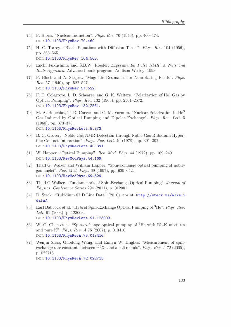
Bibliography
[74] F. Bloch. “Nuclear Induction”. Phys. Rev. 70 (1946), pp. 460–474.doi: 10.1103/PhysRev.70.460.
[75] H. C. Torrey. “Bloch Equations with Diffusion Terms”. Phys. Rev. 104 (1956),pp. 563–565.doi: 10.1103/PhysRev.104.563.
[76] Eiichi Fukushima and S.B.W. Roeder. Experimental Pulse NMR: A Nuts andBolts Approach. Advanced book program. Addison-Wesley, 1993.
[77] F. Bloch and A. Siegert. “Magnetic Resonance for Nonrotating Fields”. Phys.Rev. 57 (1940), pp. 522–527.doi: 10.1103/PhysRev.57.522.
[78] F. D. Colegrove, L. D. Schearer, and G. K. Walters. “Polarization of He3 Gas byOptical Pumping”. Phys. Rev. 132 (1963), pp. 2561–2572.doi: 10.1103/PhysRev.132.2561.
[79] M. A. Bouchiat, T. R. Carver, and C. M. Varnum. “Nuclear Polarization in He3
Gas Induced by Optical Pumping and Dipolar Exchange”. Phys. Rev. Lett. 5(1960), pp. 373–375.doi: 10.1103/PhysRevLett.5.373.
[80] B. C. Grover. “Noble-Gas NMR Detection through Noble-Gas-Rubidium Hyper-fine Contact Interaction”. Phys. Rev. Lett. 40 (1978), pp. 391–392.doi: 10.1103/PhysRevLett.40.391.
[81] W. Happer. “Optical Pumping”. Rev. Mod. Phys. 44 (1972), pp. 169–249.doi: 10.1103/RevModPhys.44.169.
[82] Thad G. Walker and William Happer. “Spin-exchange optical pumping of noble-gas nuclei”. Rev. Mod. Phys. 69 (1997), pp. 629–642.doi: 10.1103/RevModPhys.69.629.
[83] Thad G Walker. “Fundamentals of Spin-Exchange Optical Pumping”. Journal ofPhysics: Conference Series 294 (2011), p. 012001.
[84] D. Steck. “Rubidium 87 D Line Data” (2010). eprint: http://steck.us/alkalidata/.
[85] Earl Babcock et al. “Hybrid Spin-Exchange Optical Pumping of 3He”. Phys. Rev.Lett. 91 (2003), p. 123003.doi: 10.1103/PhysRevLett.91.123003.
[86] W. C. Chen et al. “Spin-exchange optical pumping of 3He with Rb-K mixturesand pure K”. Phys. Rev. A 75 (2007), p. 013416.doi: 10.1103/PhysRevA.75.013416.
[87] Wenjin Shao, Guodong Wang, and Emlyn W. Hughes. “Measurement of spin-exchange rate constants between 129Xe and alkali metals”. Phys. Rev. A 72 (2005),p. 022713.doi: 10.1103/PhysRevA.72.022713.
133
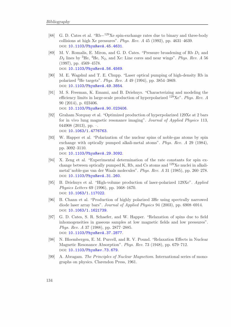
Bibliography
[88] G. D. Cates et al. “Rb−129Xe spin-exchange rates due to binary and three-bodycollisions at high Xe pressures”. Phys. Rev. A 45 (1992), pp. 4631–4639.doi: 10.1103/PhysRevA.45.4631.
[89] M. V. Romalis, E. Miron, and G. D. Cates. “Pressure broadening of Rb D1 andD2 lines by 3He, 4He, N2, and Xe: Line cores and near wings”. Phys. Rev. A 56(1997), pp. 4569–4578.doi: 10.1103/PhysRevA.56.4569.
[90] M. E. Wagshul and T. E. Chupp. “Laser optical pumping of high-density Rb inpolarized 3He targets”. Phys. Rev. A 49 (1994), pp. 3854–3869.doi: 10.1103/PhysRevA.49.3854.
[91] M. S. Freeman, K. Emami, and B. Driehuys. “Characterizing and modeling theefficiency limits in large-scale production of hyperpolarized 129Xe”. Phys. Rev. A90 (2014), p. 023406.doi: 10.1103/PhysRevA.90.023406.
[92] Graham Norquay et al. “Optimized production of hyperpolarized 129Xe at 2 barsfor in vivo lung magnetic resonance imaging”. Journal of Applied Physics 113,044908 (2013), pp. –.doi: 10.1063/1.4776763.
[93] W. Happer et al. “Polarization of the nuclear spins of noble-gas atoms by spinexchange with optically pumped alkali-metal atoms”. Phys. Rev. A 29 (1984),pp. 3092–3110.doi: 10.1103/PhysRevA.29.3092.
[94] X. Zeng et al. “Experimental determination of the rate constants for spin ex-change between optically pumped K, Rb, and Cs atoms and 129Xe nuclei in alkali-metal˘noble-gas van der Waals molecules”. Phys. Rev. A 31 (1985), pp. 260–278.doi: 10.1103/PhysRevA.31.260.
[95] B. Driehuys et al. “High-volume production of laser-polarized 129Xe”. AppliedPhysics Letters 69 (1996), pp. 1668–1670.doi: 10.1063/1.117022.
[96] B. Chann et al. “Production of highly polarized 3He using spectrally narroweddiode laser array bars”. Journal of Applied Physics 94 (2003), pp. 6908–6914.doi: 10.1063/1.1621739.
[97] G. D. Cates, S. R. Schaefer, and W. Happer. “Relaxation of spins due to fieldinhomogeneities in gaseous samples at low magnetic fields and low pressures”.Phys. Rev. A 37 (1988), pp. 2877–2885.doi: 10.1103/PhysRevA.37.2877.
[98] N. Bloembergen, E. M. Purcell, and R. V. Pound. “Relaxation Effects in NuclearMagnetic Resonance Absorption”. Phys. Rev. 73 (1948), pp. 679–712.doi: 10.1103/PhysRev.73.679.
[99] A. Abragam. The Principles of Nuclear Magnetism. International series of mono-graphs on physics. Clarendon Press, 1961.
134
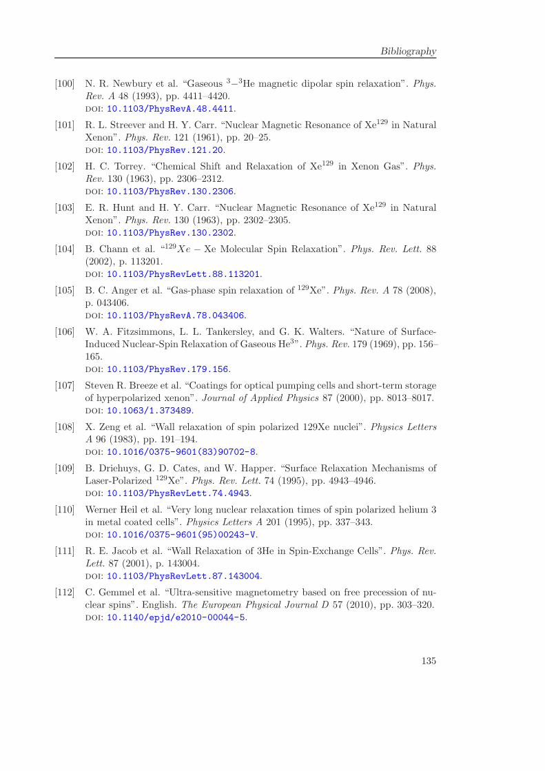
Bibliography
[100] N. R. Newbury et al. “Gaseous 3−3He magnetic dipolar spin relaxation”. Phys.Rev. A 48 (1993), pp. 4411–4420.doi: 10.1103/PhysRevA.48.4411.
[101] R. L. Streever and H. Y. Carr. “Nuclear Magnetic Resonance of Xe129 in NaturalXenon”. Phys. Rev. 121 (1961), pp. 20–25.doi: 10.1103/PhysRev.121.20.
[102] H. C. Torrey. “Chemical Shift and Relaxation of Xe129 in Xenon Gas”. Phys.Rev. 130 (1963), pp. 2306–2312.doi: 10.1103/PhysRev.130.2306.
[103] E. R. Hunt and H. Y. Carr. “Nuclear Magnetic Resonance of Xe129 in NaturalXenon”. Phys. Rev. 130 (1963), pp. 2302–2305.doi: 10.1103/PhysRev.130.2302.
[104] B. Chann et al. “129Xe − Xe Molecular Spin Relaxation”. Phys. Rev. Lett. 88(2002), p. 113201.doi: 10.1103/PhysRevLett.88.113201.
[105] B. C. Anger et al. “Gas-phase spin relaxation of 129Xe”. Phys. Rev. A 78 (2008),p. 043406.doi: 10.1103/PhysRevA.78.043406.
[106] W. A. Fitzsimmons, L. L. Tankersley, and G. K. Walters. “Nature of Surface-Induced Nuclear-Spin Relaxation of Gaseous He3”. Phys. Rev. 179 (1969), pp. 156–165.doi: 10.1103/PhysRev.179.156.
[107] Steven R. Breeze et al. “Coatings for optical pumping cells and short-term storageof hyperpolarized xenon”. Journal of Applied Physics 87 (2000), pp. 8013–8017.doi: 10.1063/1.373489.
[108] X. Zeng et al. “Wall relaxation of spin polarized 129Xe nuclei”. Physics LettersA 96 (1983), pp. 191–194.doi: 10.1016/0375-9601(83)90702-8.
[109] B. Driehuys, G. D. Cates, and W. Happer. “Surface Relaxation Mechanisms ofLaser-Polarized 129Xe”. Phys. Rev. Lett. 74 (1995), pp. 4943–4946.doi: 10.1103/PhysRevLett.74.4943.
[110] Werner Heil et al. “Very long nuclear relaxation times of spin polarized helium 3in metal coated cells”. Physics Letters A 201 (1995), pp. 337–343.doi: 10.1016/0375-9601(95)00243-V.
[111] R. E. Jacob et al. “Wall Relaxation of 3He in Spin-Exchange Cells”. Phys. Rev.Lett. 87 (2001), p. 143004.doi: 10.1103/PhysRevLett.87.143004.
[112] C. Gemmel et al. “Ultra-sensitive magnetometry based on free precession of nu-clear spins”. English. The European Physical Journal D 57 (2010), pp. 303–320.doi: 10.1140/epjd/e2010-00044-5.
135
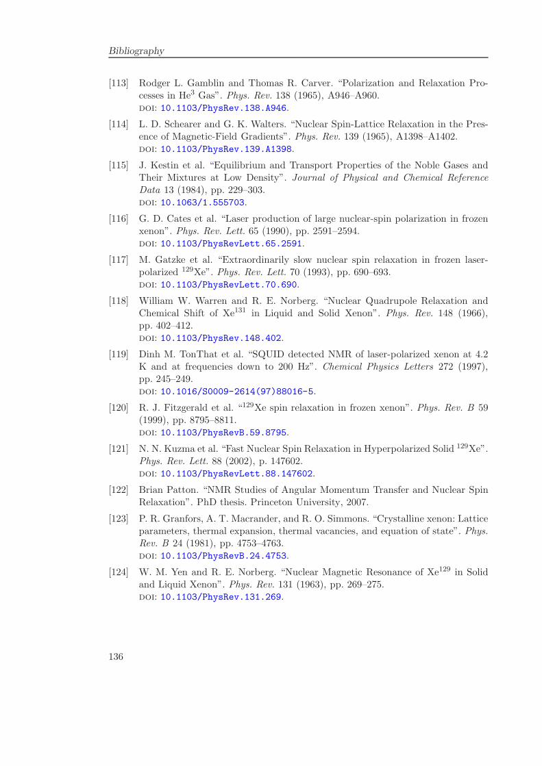
Bibliography
[113] Rodger L. Gamblin and Thomas R. Carver. “Polarization and Relaxation Pro-cesses in He3 Gas”. Phys. Rev. 138 (1965), A946–A960.doi: 10.1103/PhysRev.138.A946.
[114] L. D. Schearer and G. K. Walters. “Nuclear Spin-Lattice Relaxation in the Pres-ence of Magnetic-Field Gradients”. Phys. Rev. 139 (1965), A1398–A1402.doi: 10.1103/PhysRev.139.A1398.
[115] J. Kestin et al. “Equilibrium and Transport Properties of the Noble Gases andTheir Mixtures at Low Density”. Journal of Physical and Chemical ReferenceData 13 (1984), pp. 229–303.doi: 10.1063/1.555703.
[116] G. D. Cates et al. “Laser production of large nuclear-spin polarization in frozenxenon”. Phys. Rev. Lett. 65 (1990), pp. 2591–2594.doi: 10.1103/PhysRevLett.65.2591.
[117] M. Gatzke et al. “Extraordinarily slow nuclear spin relaxation in frozen laser-polarized 129Xe”. Phys. Rev. Lett. 70 (1993), pp. 690–693.doi: 10.1103/PhysRevLett.70.690.
[118] William W. Warren and R. E. Norberg. “Nuclear Quadrupole Relaxation andChemical Shift of Xe131 in Liquid and Solid Xenon”. Phys. Rev. 148 (1966),pp. 402–412.doi: 10.1103/PhysRev.148.402.
[119] Dinh M. TonThat et al. “SQUID detected NMR of laser-polarized xenon at 4.2K and at frequencies down to 200 Hz”. Chemical Physics Letters 272 (1997),pp. 245–249.doi: 10.1016/S0009-2614(97)88016-5.
[120] R. J. Fitzgerald et al. “129Xe spin relaxation in frozen xenon”. Phys. Rev. B 59(1999), pp. 8795–8811.doi: 10.1103/PhysRevB.59.8795.
[121] N. N. Kuzma et al. “Fast Nuclear Spin Relaxation in Hyperpolarized Solid 129Xe”.Phys. Rev. Lett. 88 (2002), p. 147602.doi: 10.1103/PhysRevLett.88.147602.
[122] Brian Patton. “NMR Studies of Angular Momentum Transfer and Nuclear SpinRelaxation”. PhD thesis. Princeton University, 2007.
[123] P. R. Granfors, A. T. Macrander, and R. O. Simmons. “Crystalline xenon: Latticeparameters, thermal expansion, thermal vacancies, and equation of state”. Phys.Rev. B 24 (1981), pp. 4753–4763.doi: 10.1103/PhysRevB.24.4753.
[124] W. M. Yen and R. E. Norberg. “Nuclear Magnetic Resonance of Xe129 in Solidand Liquid Xenon”. Phys. Rev. 131 (1963), pp. 269–275.doi: 10.1103/PhysRev.131.269.
136
Bibliography
[125] C A Sholl. “Nuclear spin relaxation by transitional diffusion in solids. XII. Ananalytical approximation”. Journal of Physics C: Solid State Physics 21 (1988),p. 319.
[126] K.L. Sauer, R.J. Fitzgerald, and W. Happer. “Laser-polarized liquid xenon”.Chemical Physics Letters 277 (1997), pp. 153–158.doi: 10.1016/S0009-2614(97)00876-2.
[127] M. V. Romalis et al. “New Limit on the Permanent Electric Dipole Moment of199Hg”. Phys. Rev. Lett. 86 (2001), pp. 2505–2508.doi: 10.1103/PhysRevLett.86.2505.
[128] K. L. Sauer et al. “NMR instabilities and spectral clustering in laser-polarizedliquid xenon”. Phys. Rev. B 63 (2001), p. 184427.doi: 10.1103/PhysRevB.63.184427.
[129] J. Jeener. “Dynamical Effects of the Dipolar Field Inhomogeneities in High-Resolution NMR: Spectral Clustering and Instabilities”. Phys. Rev. Lett. 82 (1999),pp. 1772–1775.doi: 10.1103/PhysRevLett.82.1772.
[130] M. P. Ledbetter and M. V. Romalis. “Nonlinear Effects from Dipolar Interactionsin Hyperpolarized Liquid 129Xe”. Phys. Rev. Lett. 89 (2002), p. 287601.doi: 10.1103/PhysRevLett.89.287601.
[131] M. D. Swallows et al. “Techniques used to search for a permanent electric dipolemoment of the 199Hg atom and the implications for CP violation”. Phys. Rev. A87 (2013), p. 012102.doi: 10.1103/PhysRevA.87.012102.
[132] A. Yoshimi et al. “Nuclear Spin Maser Oscillation of 129Xe by Means of Optical-Detection Feedback”. English. Hyperfine Interactions 159 (2004), pp. 401–405.doi: 10.1007/s10751-005-9132-1.
[133] Tapani Ryhanen et al. “SQUID magnetometers for low-frequency applications”.English. Journal of Low Temperature Physics 76 (1989), pp. 287–386.doi: 10.1007/BF00681735.
[134] R. L. Fagaly. “Superconducting quantum interference device instruments andapplications”. Review of Scientific Instruments 77, 101101 (2006), pp. –.doi: 10.1063/1.2354545.
[135] J. Clarke and A.I. Braginski. The SQUID Handbook: Fundamentals and Technol-ogy of SQUIDs and SQUID Systems. The SQUID Handbook. Wiley, 2004.
[136] M. Tinkham. Introduction to Superconductivity: Second Edition. Dover Books onPhysics. Dover Publications, 2004.
[137] W. Buckel and R. Kleiner. Supraleitung: Grundlagen und Anwendungen. LehrbuchPhysik. Wiley, 2013.
137
Bibliography
[138] W. Meissner and R. Ochsenfeld. “Ein neuer Effekt bei Eintritt der Supraleitfahigkeit”.German. Naturwissenschaften 21 (1933), pp. 787–788.doi: 10.1007/BF01504252.
[139] B.D. Josephson. “Possible new effects in superconductive tunnelling”. PhysicsLetters 1 (1962), pp. 251–253.doi: 10.1016/0031-9163(62)91369-0.
[140] R.P. Feynman, R.B. Leighton, and M. Sands. The Feynman Lectures on Physics:Quantum Mechanics. Basic Books. Basic Books, 2011.
[141] A Yoshimi et al. “Nuclear spin maser with an artificial feedback mechanism”.Physics Letters A 304 (2002), pp. 13–20.doi: 10.1016/S0375-9601(02)01324-5.
[142] A. Yoshimi et al. “Low-frequency 129Xe nuclear spin oscillator with optical spindetection”. Physics Letters A 376 (2012), pp. 1924–1929.doi: 10.1016/j.physleta.2012.04.043.
[143] D. Budker and M. Romalis. “Optical magnetometry”. Nature Physics 3 (2007),pp. 227–234.doi: 10.1038/nphys566.
[144] Yannis K. Semertzidis. “A Storage Ring proton Electric Dipole Moment exper-iment: most sensitive experiment to CP-violation beyond the Standard Model”(2011). arXiv: 1110.3378 [physics.acc-ph].
[145] Stephen E. Derenzo et al. “Electron avalanche in liquid xenon”. Phys. Rev. A 9(1974), pp. 2582–2591.doi: 10.1103/PhysRevA.9.2582.
[146] C. Ciofi et al. “Ultra low noise current sources”. Instrumentation and Measure-ment Technology Conference, 1997. IMTC/97. Proceedings. Sensing, Processing,Networking., IEEE. Vol. 2. 1997, pp. 1486–1489.doi: 10.1109/IMTC.1997.612447.
[147] J. M. Pendlebury et al. “Geometric-phase-induced false electric dipole momentsignals for particles in traps”. Phys. Rev. A 70 (2004), p. 032102.doi: 10.1103/PhysRevA.70.032102.
[148] W. Feldmeier. “Numerical investigation of a new 129Xe EDM experiment”. Diplomathesis. TU Munchen, 2010.
[149] F. Baudenbacher, N. T. Peters, and J. P. Wikswo. “High resolution low-temperaturesuperconductivity superconducting quantum interference device microscope forimaging magnetic fields of samples at room temperatures”. Review of ScientificInstruments 73 (2002), pp. 1247–1254.doi: 10.1063/1.1448142.
[150] B. Taubenheim. “Towards a New 129 Xenon EDM Experiment”. Diploma thesis.TU Munchen, 2011.
138
Bibliography
[151] Karsten Tell. “Developments for efficient transport of hyperpolarized 129Xe”.Diploma thesis. TU Munchen, 2014.
[152] Max Newrzella. “Calculation of a low-field NMR system for the XEDM experi-ment”. Bachelor thesis. TU Munchen, 2011.
[153] David Wurm. “Development of a gas-flow cooling system for a new measurementof the electric dipole moment of 129Xe”. Bachelor thesis. TU Munchen, 2012.
[154] I. Altarev et al. “A magnetically shielded room with ultra low residual field andgradient”. Review of Scientific Instruments 85, 075106 (2014), pp. –.doi: 10.1063/1.4886146.
[155] M. Burghoff et al. “A vector magnetometer module for biomagnetic application”.Applied Superconductivity, IEEE Transactions on 9 (1999), pp. 4069–4072.doi: 10.1109/77.783920.
[156] V.A. Dzuba, V.V. Flambaum, and P.G. Silvestrov. “Bounds on electric dipolemoments and T-violating weak interactions of the nucleons”. Physics Letters B154 (1985), pp. 93–95.doi: 10.1016/0370-2693(85)90564-7.
[157] V. Flambaum and I. Khriplovich. “New bounds on the electric dipole momentof the electron and on T-odd electron-nucleon coupling”. Sov. Phys. JETP 62(1985), p. 872.
[158] K. C. Hasson et al. “Spin relaxation due to magnetic-field inhomogeneities: Quar-tic dependence and diffusion-constant measurements”. Phys. Rev. A 41 (1990),pp. 3672–3688.doi: 10.1103/PhysRevA.41.3672.
[159] R. H. Acosta et al. “Diffusion in binary gas mixtures studied by NMR of hyper-polarized gases and molecular dynamics simulations”. Phys. Chem. Chem. Phys.8 (2006), pp. 4182–4188.doi: 10.1039/B609316G.
[160] C. B. Alcock, V. P. Itkin, and M. K. Horrigan. “Vapour Pressure Equations forthe Metallic Elements: 298–2500K”. Canadian Metallurgical Quarterly 23 (1984),pp. 309–313.doi: 10.1179/cmq.1984.23.3.309.
139

Acknowledgements
I want to thank Prof. Dr. Peter Fierlinger, who trustfully received me in his very younggroup and got me into this fascinating field of physics. His enthusiastic character andinspiration feeds our work with new ideas and creates a productive and pleasant atmo-sphere.I’m also particularly grateful to Jaideep Singh for guiding the last year of my thesis,his help in the lab and setting up most of the He/Xe equipment. Not to forget thenight-shifts reading the thesis and sending comments.The whole group needs to be thanked for the mutual support and humor, in particu-lar the many students that contributed to the liquid xenon EDM: Wolfhart Feldmeier,Max Newrzella, Felix Rosenau, Stephanie Seidl, Ann-Katrin Straub, Bernd Taubenheim,Karsten Tell, David Wurm.The great accomplishments of the He/Xe clock-comparison were only possible with thecooperation of many people from the University of Michigan, Michigan State, PTB Berlinand the MLZ in Garching, namely Tim Chupp, Skyler Degenkolb, Natasha Sachdeva,Fei Gong, Jaideep Singh, Wolfgang Kilian, Allard Schnabel, Silvia Knappe-Gruneberg,Jens Voigt, Isaac Fan, Earl Babcock, Martin Burghoff and the support of all our stu-dents, particularly Eva Krageloh and Jonas Meinel.
A special thanks goes to staff at the mechanics workshop, particularly Michael Novotnyand Thomas Deuschle and the glass blowing staff in the chemistry department. All ofwhich did their best to produce urgently needed parts or fix broken glassware.For their helpfulness in many aspects I want to thank the administration staff of theexcellence cluster, Karin Frank and Rainer Stoepler.A big thanks goes to Andi Weiss, who talked me into biking to Garching every day andsupported urgent bike repairs any time.
I thank my partents and my sister for their lifelong support, motivation and kindness.To conclude, I’m particularly grateful to Verena, who supported me with encouragementand patience throughout the last years.
141