ii

공학박사학위논문

Evaluation of Ultimate Compressive Strengthof Flanges Stiffened with U-ribs

in Wide Steel Box-girder

U리브로 보강된 광폭 강박스거더 플랜지의극한압축강도 평가

2015년 8월

서울대학교 대학원

건설환경공학부

김 종 서

iii

ABSTRACT

This study proposes a method to evaluate the in-plane ultimate compressive

strength of stiffened flanges with U-ribs in a wide steel box-girder. When a pri-

mary bending moment and/or an axial force are applied to the steel box-girder, the

main load component of top or bottom flanges is longitudinal in-plane axial com-

pression. For the reason above, the stiffened flanges with U-ribs are separated

from the box-girder and modeled by finite elements with idealized boundary con-

ditions.

Generally, the stiffened flanges between diaphragms are designed to behave as

if simple support conditions were applied. If the diaphragms are stiff (thick)

enough in the out of plane direction, loaded edges of the stiffened flanges will have

the same displacement in longitudinal direction. This condition can be analyzed

by displacement control. However, if the diaphragms are flexible (thin) enough in

the out of plane direction, all parts of the loaded edges of the stiffened flanges will

have different displacements in the longitudinal direction. This condition has to

be analyzed by force control. Thus, the ultimate compressive strengths of the

stiffened flanges are evaluated considering effects of the bending stiffness of the

diaphragms on in-plane behaviors of the stiffened flange. This study shows that

the effect of the diaphragm is negligible under the practical thickness. Thus, the

force control is considered to be more appropriate than the displacement control for

iv

evaluation of the ultimate compressive strength of flanges stiffened with U-ribs.

Based on the ultimate compressive strengths in the force control, a strength for-

mula is proposed.

The FHWA (Federal Highway Administration) provisions are reviewed and

evaluated in terms of the finite element solution in this study. The FHWA provi-

sions accurately estimate the ultimate compressive strengths of the stiffened

flanges in the force control. The ultimate compressive strengths from the FHWA

provisions are nearly the same as those from the proposed strength formula.

Thus, this study recommends the proposed strength formula or the FHWA

provisions for evaluation of the ultimate compressive strength of stiffened flanges

with U-ribs. Either way, the ultimate compressive strengths are almost same.

Key Words:

Wide steel box-girder, Ultimate compressive strength, Stiffened flange, U-rib,

Bending stiffness of diaphragm, Force control, Displacement control, FHWA pro-

visions

Student Number: 2009-30938

v

Table of Contents

ABSTRACT ................................................................................III

1. INTRODUCTION.................................................................... 1

2. NUMERICAL METHODS FOR EVALUATION OF

ULTIMATE COMPRESSIVE STRENGTH............................. 9

2.1 In-plane ultimate compressive strength ..........................................12

2.2 Theory of small deformation plasticity in stiffened flanges ...........14

2.3 Finite element modeling of stiffened flanges with U-ribs ..............47

2.4 Initial geometric imperfection.........................................................57

2.5 Residual stress and recovery of its effect ........................................61

2.6 Force control and displacement control ..........................................66

2.7 Modeling of diaphragms .................................................................70

2.8 Proposed method for evaluation of ultimate compressive strength

of stiffened flanges with U-ribs.......................................................73

2.9 Verification to finite element scheme..............................................76

vi

3. ULTIMATE COMPRESSIVE STRENGTH OF

STIFFENED FLANGES WITH U-RIBS ................................ 79

3.1 Effect of bending stiffness of diaphragms on in-plane behaviors of

stiffened flanges with U-ribs ...........................................................81

3.2 Differences between behaviors of stiffened flanges in force control

and displacement control.................................................................87

3.3 Strengths and behaviors of stiffened flanges with U-ribs ...............94

3.4 Influence of initial geometric imperfection...................................103

3.5 Influence of residual stresses ........................................................108

3.6 Snap-though like phenomenon in stiffened flanges with U-ribs... 113

3.7 Proposed strength formula for stiffened flanges with U-ribs........127

3.8 Evaluation of proposed strength formula based on statistics ........143

3.9 Ultimate compressive strength based on probability distribution of

random variable.............................................................................154

4. VALIDITY OF CURRENT DESIGN CODE ‘FHWA

PROVISIONS’.......................................................................... 157

4.1 Philosophy and basic assumptions ................................................159

4.2 Ultimate compressive strength by the interaction diagram

method...........................................................................................164

vii

4.3 Evaluation of ultimate compressive strength of stiffened flanges by

the FHWA provisions ....................................................................167

4.4 Applicability of the FHWA provisions to HSB600 steel and

SM570 steel...................................................................................178

5. CONCLUSIONS AND FURTHER STUDY...................... 182

REFERENCES......................................................................... 188

viii

List of Figures

FIG. 1.1 WIDE-TYPE STEEL BOX-GIRDER USED IN CABLE-SUPPORTED BRIDGES. ......................1

FIG. 2.1 LOAD-DISPLACEMENT CURVE OF STIFFENED THIN FLANGE ......................................13

FIG. 2.2 AVERAGE VALUES OF EFFECTIVE PLASTIC STRAIN AT THE ULTIMATE STATES OF

STIFFENED FLANGES.......................................................................................................15

FIG. 2.3 TWO DIFFERENT TYPES OF HARDENING MODEL........................................................23

FIG. 2.4 RADIAL RETURN MAPPING METHOD FOR ISOTROPIC HARDENING.............................27

FIG. 2.5 VERIFICATION TESTS FOR THE NLGEOM OPTION IN ABAQUS .................................40

FIG. 2.6 RIKS METHOD (RIKS AND WEMPNER) .....................................................................46

FIG. 2.7 MODIFIED RIKS METHOD (FRIED METHOD).............................................................46

FIG. 2.8 ASSUMED STRESS-STRAIN RELATIONSHIP OF CONVENTIONAL STEEL. ......................48

FIG. 2.9 IDEALIZED BOUNDARY CONDITION OF STIFFENED FLANGE WITH 10 U-RIBS ............49

FIG. 2.10 GEOMETRY OF HYPOTHETICAL MODEL ..................................................................51

FIG. 2.11 REQUIRED STIFFENERS IN WIDE STIFFENED FLANGES.............................................52

FIG. 2.12 TRACING POINT FOR LONGITUDINAL DISPLACEMENT IN MESH CONVERGENCE TEST

......................................................................................................................................55

FIG. 2.13 THE NUMBER OF MESHES CUT INTO EQUALLY SPACED 32 DIVISIONS IN

LONGITUDINAL DIRECTION.............................................................................................56

FIG. 2.14 LONGITUDINAL DISPLACEMENT VERSUS THE NUMBER OF MESHES.........................56

FIG. 2.15 INITIAL GEOMETRIC IMPERFECTION SHAPES ..........................................................60

FIG. 2.16 ASSUMED RESIDUAL STRESS DISTRIBUTION PATTERN.............................................62

FIG. 2.17 CROSS SECTION FOR PRELIMINARY STUDY.............................................................64

ix

FIG. 2.18 NORMALIZED LOAD-DISPLACEMENT CURVES FOR VERIFICATION OF DEFORMATION

RECOVERY METHOD .......................................................................................................65

FIG. 2.19 DESCRIPTION OF COMPRESSION TEST BY (A) FORCE CONTROL AND (B)

DISPLACEMENT CONTROL..............................................................................................66

FIG. 2.20 BENDING STIFFNESS OF DIAPHRAGM AND AXIAL STIFFNESS OF STIFFENED FLANGE

WITH 10 URIBS ..............................................................................................................69

FIG. 2.21 FIXED END FORCES WITH RESPECT TO PRESCRIBED DISPLACEMENT IN

DIAPHRAGM ...................................................................................................................69

FIG. 2.22 MODELING OF DIAPHRAGMS USING BEAM ELEMENT AND RIGID LINK ....................71

FIG. 2.23 MODELING OF STIFFENED FLANGE AND DIAPHRAGMS IN ABAQUS ......................72

FIG. 2.24 PROCEDURE FOR EVALUATION OF ULTIMATE COMPRESSIVE STRENGTH..................75

FIG. 2.25 CROSS SECTION OF CHOU’S MODEL FOR VERIFICATION..........................................76

FIG. 2.26 LOAD-DISPLACEMENT CURVE BY VERIFICATION STUDY .........................................77

FIG. 3.1 RATIOS OF BENDING STIFFNESS OF DIAPHRAGMS AGAINST AXIAL STIFFNESS OF

STIFFENED FLANGES VERSUS THICKNESS OF DIAPHRAGMS.............................................81

FIG. 3.2 LOAD-DISPLACEMENT CURVES IN CASE 2................................................................83

FIG. 3.3 LOAD-DISPLACEMENT CURVES IN CASE 5................................................................84

FIG. 3.4 LOAD-DISPLACEMENT CURVES IN CASE 8................................................................85

FIG. 3.5 LONGITUDINAL DISPLACEMENTS AND LONGITUDINAL STRESSES AT FLANGE-EDGE IN

CASE 2 ...........................................................................................................................90

FIG. 3.6 LONGITUDINAL DISPLACEMENTS AND LONGITUDINAL STRESSES AT FLANGE-EDGE IN

CASE 5 ...........................................................................................................................91

FIG. 3.7 LONGITUDINAL DISPLACEMENTS AND LONGITUDINAL STRESSES AT FLANGE-EDGE IN

CASE 8 ...........................................................................................................................92

x

FIG. 3.8 AVERAGE STRESS RATIOS OF U-RIBS-EDGES AGAINST FLANGE-EDGE IN FORCE

CONTROL AND DISPLACEMENT CONTROL .......................................................................93

FIG. 3.9 INELASTIC BUCKLING MODES OF FLANGES STIFFENED WITH U-RIB AT ULTIMATE AND

FRACTURE STATES ..........................................................................................................97

FIG. 3.10 SIMPLIFIED INELASTIC BUCKLING MODES ..............................................................99

FIG. 3.11 MINIMUM STRENGTH LINES WITH RESPECT TO PLATE SLENDERNESS PARAMETER IN

FORCE CONTROL ..........................................................................................................101

FIG. 3.12 MINIMUM STRENGTH LINES WITH RESPECT TO PLATE SLENDERNESS PARAMETER IN

DISPLACEMENT CONTROL.............................................................................................101

FIG. 3.13 MINIMUM STRENGTH LINES WITH RESPECT TO COLUMN SLENDERNESS PARAMETER

IN FORCE CONTROL ......................................................................................................102

FIG. 3.14 MINIMUM STRENGTH LINES WITH RESPECT TO COLUMN SLENDERNESS PARAMETER

IN DISPLACEMENT CONTROL ........................................................................................102

FIG. 3.15 INFLUENCE OF INITIAL GEOMETRIC IMPERFECTION SHAPES ON ULTIMATE

COMPRESSIVE STRENGTH OF SERIES P07. .....................................................................104

FIG. 3.16 VERTICAL DISPLACEMENT (M) BY RESIDUAL STRESSES REDISTRIBUTION IN PERFECT

STIFFENED FLANGE (P07-C07 MODEL) ........................................................................105

FIG. 3.17 INFLUENCE OF RESIDUAL STRESS ON ULTIMATE COMPRESSIVE STRENGTH. ..........111

FIG. 3.18 COMPRESSION VERSUS LONGITUDINAL SHORTENING FOR P07-C09 MODEL IN FC6

....................................................................................................................................116

FIG. 3.19 VERTICAL DISPLACEMENT VERSUS COMPRESSION FOR P07-C09 MODEL IN FC6 .116

FIG. 3.20 HISTORY OF VERTICAL LOCATIONS AT (A) LONGITUDINAL CENTERLINE AND (B)

TRANSVERSE CENTERLINE OF P07-C09 MODEL IN FC6................................................117

FIG. 3.21 YIELDING AREA OF P07-C09 MODEL IN FC6........................................................118

xi

FIG. 3.22 COMPRESSION VERSUS LONGITUDINAL SHORTENING FOR P07-C09 MODEL IN DC5

....................................................................................................................................119

FIG. 3.23 VERTICAL DISPLACEMENT VERSUS COMPRESSION FOR P07-C09 MODEL IN DC5 119

FIG. 3.24 HISTORY OF VERTICAL LOCATIONS AT (A) LONGITUDINAL CENTERLINE AND (B)

TRANSVERSE CENTERLINE OF P07-C09 MODEL IN DC5 ...............................................120

FIG. 3.25 YIELDING AREA OF P07-C09 MODEL IN DC5. ......................................................121

FIG. 3.26 OCCURRENCE PATTERN OF SNAP-THROUGH LIKE PHENOMENON. .........................125

FIG. 3.27 VERTICAL DISPLACEMENTS BY REDISTRIBUTION EFFECT OF RESIDUAL STRESSES.

....................................................................................................................................126

FIG. 3.28 PROPOSED STRENGTH FORMULA..........................................................................132

FIG. 3.29 EVALUATION OF STRENGTHS FROM DESIGN CODES IN TERMS OF PROPOSED

STRENGTH FORMULA (THICK FLANGE, 3.0pl ) ......................................................137

FIG. 3.30 EVALUATION OF STRENGTHS FROM DESIGN CODES IN TERMS OF PROPOSED

STRENGTH FORMULA (INTERMEDIATE FLANGE, 7.0pl ) ........................................138

FIG. 3.31 EVALUATION OF STRENGTHS FROM DESIGN CODES IN TERMS OF PROPOSED

STRENGTH FORMULA (THIN FLANGE, 3.1pl ).........................................................139

FIG. 3.32 EVALUATION OF STRENGTHS FROM DESIGN CODES IN TERMS PROPOSED STRENGTH

FORMULA (SHORT FLANGE, 3.0col ) ......................................................................140

FIG. 3.33 EVALUATION OF STRENGTHS FROM DESIGN CODES IN TERMS PROPOSED STRENGTH

FORMULA (INTERMEDIATE FLANGE, 7.0col ) .........................................................141

FIG. 3.34 EVALUATION OF STRENGTHS FROM DESIGN CODES IN TERMS PROPOSED STRENGTH

FORMULA (LONG FLANGE, 3.1col ) ........................................................................142

xii

FIG. 3.35 STATISTICAL INTERPRETATION OF STRENGTHS IN NINE ANALYSIS CASES..............144

FIG. 3.36 STATISTICAL EVALUATION OF PROPOSED STRENGTH FORMULA BASED ON FEA

RESULTS AT 3.0col ..............................................................................................148

FIG. 3.37 STATISTICAL EVALUATION OF PROPOSED STRENGTH FORMULA BASED ON FEA

RESULTS AT 5.0col ..............................................................................................149

FIG. 3.38 STATISTICAL EVALUATION OF PROPOSED STRENGTH FORMULA BASED ON FEA

RESULTS AT 7.0col ..............................................................................................150

FIG. 3.39 STATISTICAL EVALUATION OF PROPOSED STRENGTH FORMULA BASED ON FEA

RESULTS AT 9.0col ..............................................................................................151

FIG. 3.40 STATISTICAL EVALUATION OF PROPOSED STRENGTH FORMULAS BASED ON FEA

RESULTS AT 1.1col ...............................................................................................152

FIG. 3.41 STATISTICAL EVALUATION OF PROPOSED STRENGTH FORMULA BASED ON FEA

RESULTS AT 3.1col ...............................................................................................153

FIG. 4.1 GEOMETRY FOR (A) COLUMN-LIKE BEHAVIOR AND (B) PLATE-LIKE BEHAVIOR IN

FLANGES STIFFENED WITH OPEN-TYPE STIFFENERS UNDER THE STRUT APPROACH .......160

FIG. 4.2 GEOMETRY FOR (A) COLUMN-LIKE BEHAVIOR AND (B) PLATE-LIKE BEHAVIOR IN

FLANGES STIFFENED WITH CLOSED-TYPE STIFFENERS UNDER THE STRUT APPROACH ...160

FIG. 4.3 THE INTERACTION DIAGRAM BETWEEN COLUMN-TYPE BUCKLING AND PLATE-TYPE

BUCKLING (DAS, 1978)...............................................................................................161

FIG. 4.4 THE INTERACTION DIAGRAM BETWEEN COLUMN-TYPE BUCKLING AND PLATE-TYPE

BUCKLING (FHWA, 1980) ...........................................................................................162

FIG. 4.5 INVESTIGATED RANGES OF SLENDERNESS PARAMETERS ........................................167

xiii

FIG. 4.6 COMPARISON OF FEA RESULTS WITH STRENGTHS BY FHWA ................................169

FIG. 4.7 COMPARISON OF FEA RESULTS WITH STRENGTHS BY FHWA. ...............................170

FIG. 4.8 STRENGTH COMPARISON OF FHWA WITH EUROCODE3, KHBDC-CSB, PROPOSED

FORMULAS AND FEA ...................................................................................................173

FIG. 4.9 STRENGTH COMPARISON OF FHWA WITH EUROCODE3, KHBDC-CSB, PROPOSED

FORMULAS AND FEA ...................................................................................................174

FIG. 4.10 TWO DIMENSIONAL AND THREE DIMENSIONAL INTERACTION DIAGRAM OF

PROPOSED STRENGTH FORMULA (FC) ..........................................................................176

FIG. 4.11 TWO DIMENSIONAL AND THREE DIMENSIONAL INTERACTION DIAGRAM OF FHWA

PROVISIONS..................................................................................................................176

FIG. 4.12 TWO DIMENSIONAL AND THREE DIMENSIONAL INTERACTION DIAGRAMS OF

EUROCODE3.................................................................................................................177

FIG. 4.13 TWO DIMENSIONAL AND THREE DIMENSIONAL INTERACTION DIAGRAMS OF

KHBDC-CSB..............................................................................................................177

FIG. 4.14 ASSUMED STRESS-STRAIN RELATIONSHIP OF HSB600 STEEL..............................180

FIG. 4.15 ASSUMED STRESS-STRAIN RELATIONSHIP OF SM570 STEEL ................................180

FIG. 4.16 APPLICABILITY OF FHWA PROVISIONS AND PROPOSED FORMULAS TO HSB600 AND

SM570 STEEL ..............................................................................................................181

xiv

List of Tables

TABLE 2.1 VERIFICATION OF NLGEOM OPTIONS USING UNSTIFFENED FLANGE......................41

TABLE 2.2 MECHANICAL PROPERTIES OF CONVENTIONAL STEEL ..........................................48

TABLE 2.3 GEOMETRY OF U-RIB (UNIT: MM). .......................................................................51

TABLE 2.4 THICKNESS AND LONGITUDINAL LENGTH OF HYPOTHETICAL MODELS ACCORDING

TO SLENDERNESS PARAMETER........................................................................................54

TABLE 2.5. GEOMETRY AND MATERIAL PROPERTIES USED IN SHEIKH ET AL.(2002). .............64

TABLE 2.6 ANALYSIS CASES (COMBINATIONS OF IMPERFECTIONS) FOR EACH HYPOTHETICAL

MODEL. ..........................................................................................................................75

TABLE 2.7 MATERIAL PROPERTIES USED IN CHOU’S MODEL..................................................77

TABLE 3.1 ULTIMATE COMPRESSIVE STRENGTH IN FORCE CONTROL.....................................95

TABLE 3.2 ULTIMATE COMPRESSIVE STRENGTH IN DISPLACEMENT CONTROL .......................96

TABLE 3.3 INELASTIC BUCKLING MODES CORRESPONDING TO MINIMUM STRENGTHS IN FORCE

CONTROL .......................................................................................................................98

TABLE 3.4 INELASTIC BUCKLING MODES CORRESPONDING TO MINIMUM STRENGTHS IN

DISPLACEMENT CONTROL...............................................................................................98

TABLE 3.5. REDUCTION OF ULTIMATE COMPRESSIVE STRENGTH BY RESIDUAL STRESS .......112

TABLE 3.6 STRENGTH AT STARTING POINTS OF SNAP-THROUGH LIKE PHENOMENON ...........122

TABLE 3.7 COEFFICIENTS OF STRENGTH FORMULAS IN THE FORCE AND DISPLACEMENT

CONTROL .....................................................................................................................131

TABLE 3.8 STATISTICAL PROPERTIES OF PROPOSED STRENGTH FORMULA ...........................147

xv

TABLE 3.9 ASSUMPTION OF PROBABILITIES IN RESIDUAL STRESS WHILE CONSIDERING

CONTROLLED-CONDITIONS...........................................................................................155

TABLE 3.10 EXAMPLE OF ASSUMED PROBABILITY OF RESIDUAL STRESS .............................155

TABLE 4.1 MECHANICAL PROPERTIES OF HSB600 STEEL AND SM570 STEEL.....................180

1

Chapter 1

Introduction

Wide steel box-girders have been widely used in cable-supported bridges for the

past several decades. Especially, these types of girders offer a long span for the

bridges by reducing the dead weight (Petros, 1994). There is continuous progress

in construction technology and better understanding of the box-girder. Thus,

slimmer and wider box-girders are expected in the future. In recent design prac-

tice, closed type stiffeners are more preferred than open type stiffeners due to better

increase of in-plane stability and strength as well as high performance on wheel

load distribution. Fig. 1.1 shows a general wide steel box-girder used in cable-

supported bridges. When the primary bending moment (by gravity load) and/or

the axial force are applied to a box-girder, the main load component of the top or

bottom flanges are the longitudinal in-plane axial compression. Therefore, in the

general design of box-girder bridges, an important step is to evaluate the nominal

Fig. 1.1 Wide-type steel box-girder used in cable-supported bridges.

2

strengths of stiffened flanges in compression. If the nominal strengths have a

good representation of the real strengths, then we expect a rational and economical

design.

We can assume that the ultimate flexural strength of a wide steel box-girder

under the primary bending moment and/or the axial compression is contributed

only by the top or bottom flanges. Hence, this study evaluates the ultimate com-

pressive strength of stiffened flanges with U-shaped ribs (henceforth, U-ribs) in-

stead of the ultimate flexural strength of a whole box-girder.

Stiffened flanges with U-ribs have a high strength-to-weight ratio. The addi-

tion of a few stiffeners to the flanges produces a considerably stiffer system.

However, an analysis is more complicated if the stiffeners are not equally spaced or

do not have the same cross sections. Structurally, stiffened flanges consist of

many plate elements in which various inelastic buckling modes may occur. Thus,

the evaluation of the in-plane compressive strength of stiffened flanges cannot be

performed unless the behavior of stiffened flanges is clearly known. According to

classical steel box-girder theories (Ziemian, 2010), the diaphragms are designed to

be sufficiently stiff in the in-plane direction at the junction with the stiffened flange

in the box-girder. This ensures that the diaphragms provide nodal lines that act as

simple rotationally free supports to the ends of the stiffened flange. When we

consider this structural form, the failure modes of the stiffened flanges under the

uni-axial compression can be categorized into four major modes: (1) plate-type

(local) buckling between longitudinal stiffeners, (2) plate-induced column-type

3

(global) buckling of stiffened flanges with U-ribs as a unit, (3) stiffener-induced

column-type (global) buckling of stiffened flanges with U-ribs as a unit, and (4)

stiffener local buckling or stiffener tripping. Stiffener tripping mainly occurs in

open type stiffeners and rarely occurs in closed stiffeners. The ultimate strength

of stiffened flanges can usually be considered as the lowest value calculated from

the above four failure modes. If major system parameters affecting these four

modes are known, then strength curves can be approximated as a function of these

parameters. In addition, initial geometric imperfections and residual stresses are

unavoidable during the fabrication of stiffened flanges. Hence, these two imper-

fections should be taken into account. Especially, a correlation between the ulti-

mate compressive strength and redistribution effect of residual stress is one of is-

sues to reflect on.

In the past few decades, many studies have examined the ultimate compressive

strength of steel stiffened flanges (Little 1976, Mikami and Niwa 1996, Sheikh et

al. 2001, Bedair 1998). Three approaches have been mainly developed, which are

based on different philosophies. These approaches are the strut approach, ortho-

tropic plate theory and numerical methods. In the strut approach, the stiffened

flanges are considered as a series of disconnected struts, each of which consist of a

stiffener and an associated plate width. Wolchuk and Mayrbourl (1980) proposed

the interaction diagram method in the FHWA-TS-80-205 report, which is based on

the theoretical strut approach work by Little (1976). In their work, the ultimate

compressive strength is approximated implicitly and graphically as a function of

4

the elastic buckling stress and the yield stress of a strut. The FHWA-TS-80-205

report become the design code called the ‘FHWA (Federal Highway Administra-

tion) provisions’ for steel box-girders. In orthotropic plate theory, a stiffened

flange is converted into an equivalent plate with a constant thickness by smearing

out the stiffeners (Massonet et al., 1973). This method has been used in Euro-

code3 (EN 1993-1-5, 2004) for the global reduction factor to describe plate-like

behavior and column-like behavior. In numerical methods, stiffened flanges are

usually modeled and analyzed by finite elements using a commercially available

program. Many studies have shown that the finite element analysis (FEA) is a

powerful methodology for predicting the ultimate strengths and behaviors of the

structural failure (Hu 1993, Chou et al. 2006). This method has been used in Ko-

rea Highway Bridge Design Code – Cable Supported Bridge specification (MLIT,

2015) for the ultimate compressive strength of stiffened flanges.

Of the three developed design codes, the FHWA provisions has been widely

and most frequently used for over thirty years. The ‘FHWA provisions’ was de-

veloped for the open-type stiffeners, and for two grades of steel with the yield

strengths of 250MPa and 350MPa. In addition, the FHWA provisions were de-

veloped by using a strut instead of wide stiffened flanges. Thus, how accurately

the provisions predict the ultimate compressive strength of the wide stiffened

flanges with U-ribs is questionable. Whether the FHWA provisions are applicable

to high performance of steels (HPS) is also not sure.

Related studies on stiffened flanges with U-ribs have been conducted. Chen

5

et al. (2002) carried out experimental compression tests by displacement control on

two types of full-scale specimens, which represented the U-shaped stiffeners and

deck plates of a wide steel box-girder. From the test results, they proposed two

design equations based on the plate slenderness parameter for prediction of the

inelastic buckling strength of U-shape stiffeners and deck plates. In addition,

design criteria for the width-to-thickness ratio of the deck plate and U-rib stiffeners

were proposed to prevent the occurrence of premature structural failure due to local

buckling. Chou et al. (2006) conducted compression tests by displacement con-

trol on the reduced-scale orthotropic plates stiffened by closed longitudinal stiffen-

ers. The specimens simulating the top deck plates of a wide steel box-girder were

composed of a plate and three U-shaped longitudinal stiffeners. The ultimate

compressive strength and failure modes of the test specimens were compared with

test specimens used in American and Japanese design codes (AASHTO 1998, JRA

2002) and the FEA results. Especially, Chou et al. (2006) show that FEA predicts

reliable results if both initial imperfection and residual stress are considered prop-

erly. Shin et al. (2013) carried out a FEA by displacement control for in-plane

ultimate compressive strength and behavior of deck panel system in a wide steel

box-girder. The analyses included 112 stiffened flanges composed of a plate and

three U-rib stiffeners with various plate and column slenderness parameters pro-

duced from conventional or high performance steel. The results showed that the

ultimate compressive strengths are less affected by the column slenderness pa-

rameter. They also proposed strength predictor equations by the plate and column

6

slenderness parameters based on the FEA results and the safety factors with respect

to the column behavior in the Federal Highway Administration (FHWA) provisions

and Eurocode3.

The common fact of the previous studies is that the stiffened flanges were

analyzed by displacement control. If the diaphragm is stiff (thick) enough in the

out of plane direction, all parts of the loaded edges of the stiffened flanges will

have the same displacement in the longitudinal direction. Then, the stiffened

flange can be analyzed by displacement control. However, if the diaphragm is

flexible (thin) enough in the out of plane direction, displacements of the loaded

edges in the stiffened flanges will vary along the transversal axis. Then, the stiff-

ened flanges have to be analyzed by force control. Thus, the ultimate compres-

sive strengths in the force control and the displacement control can be regarded as

the lower and upper bounds, respectively. If we consider that the stiffness of a

real diaphragm in the out of plane direction is not large enough, we can expect that

the ultimate compressive strength of the stiffened flanges resides between the upper

and lower bounds.

In this study, there are two objectives. The first objective is proposition of a

method to evaluate the ultimate compressive strength of stiffened flanges with U-

ribs considering effects of diaphragms on in-plane behaviors of the stiffened flange.

The second objective is evaluation of the validity of the FHWA provisions in wide

stiffened flanges. The two objectives are researched through the topics covered in

the following chapters.

7

Chapter 2 describes theories and numerical methodologies that are used in this

study. The stiffened flanges with U-ribs are modeled by ABAQUS FEA software.

Three cases of initial geometric imprecations and three cases of residual stresses

are defined. Methodologies for force and displacement controls used in this study

are introduced. The stiffened flanges with U-ribs are analyzed by the force con-

trol and the displacement control under the same boundary conditions. To consid-

er effects of the diaphragms on in-plane behaviors of the stiffened flanges, the dia-

phragms are modeled as beam elements and are attached to the stiffened flanges

using rigid links. The assembled models are analyzed by the force control. The

analysis schemes used in this study are validated using Chou’s experimental results.

Chapter 3 shows effects of the diaphragms on the in-plane ultimate compres-

sive strengths of the stiffened flanges. Differences between behaviors of the stiff-

ened flanges in the force control and the displacement control are discussed. Ef-

fects of the initial geometric imperfections and the residual stresses on the stiffened

flanges with U-ribs are analyzed. In addition, a strength formula is proposed for

the predictions of the ultimate compressive strengths. The current design codes

(the FHWA provisions, Eurocode3 and KHBDC-CSB) are evaluated in terms of the

proposed strength formula.

Chapter 4 evaluates the validity of the FHWA provisions. The philosophy

and basic assumptions used in the provisions are discussed. The FHWA provi-

sions are compared to the FEA results of the stiffened flanges with U-ribs. For a

comparative study, Eurocode3 and KHBDC-CSB are also evaluated in terms of the

8

FEA results. Design philosophies of the current design codes are compared to

each other. The applicability of the FHWA provisions to two grades of steel with

the equivalent yield strength of 450MPa is evaluated.

Chapter 5 presents the conclusions and directions for further studies.

9

Chapter 2

Numerical methods for evaluation of ultimate com-

pressive strength

The theories and methodologies for the evaluation of the ultimate compressive

strength of stiffened flanges with U-ribs are described in chapter 2. First, defini-

tions of the ultimate compressive strength and inelastic buckling modes, which

may occur in the stiffened flanges with U-ribs, are explained. Then, an analysis

level is determined from a preliminary study. The study shows that small defor-

mation plastic theory could describe the ultimate compressive strength of the stiff-

ened flanges well. The classical plastic theory used in this study is introduced.

They are associated flow rule, isotropic hardening rule and von Mises yield criteria.

A radial return mapping algorithm is used to update the stress and plastic variable.

To consider a large rotation effect, the Green-Naghdi rate satisfying the objectivity

is introduced. Although a small strain is assumed in the plastic analysis, it is re-

garded as a large deformation problem due to the large rotation. Thus, the updat-

ed Lagrangian formulation is used. In addition, a moment amplification by an

axial force is considered. Finally, the modified Riks method is used to trace the

global equilibrium path.

The finite element software ABAQUS ver. 6-11.1 (2011) are used in this ana-

10

lysis to evaluate the ultimate compressive strength of flanges stiffened with U-ribs.

Thin shell elements consisting of quadrilateral, four node and small-strain are used

to model the stiffened flanges with U-ribs. Steel Marine 490Y (henceforth,

SM490Y) in South Korea (henceforth, Korea) Specifications for Roadway Bridges

(MLTM, 2012) is assumed for material characteristics of the stiffened flanges in

this study. An assumed model needs to well reflect the characteristic behaviors of

wide stiffened flanges. Required the minimum number of U-ribs to describe the

wideness is determined using the elastic buckling analyses. Referring to previous

studies (FHWA, 1980; Shin, 2013), hypothetical models are set up to describe two

types of behavior (plate-type buckling and column-type buckling) by proper slen-

derness parameters. The thickness of assumed stiffened flanges are determined

considering a range used in practical designs, so the sections are well proportioned.

Thus, total thirty-six hypothetical models are defined in this study. The stiffened

flanges are modeled using a sufficient number of elements. It is confirmed that a

mesh division of the model is fine enough to yield satisfactory convergence.

Plate-type buckling and column-type buckling modes (either up or down direction)

of the stiffened flanges are used based on eigenvalue analyses in order to consider

initial geometric imperfections. Fukumoto’s model (Fukumoto et al., 1974) is

applied as residual stresses to this study. Especially, the presence of redistribution

effect of residual stresses and the recovery of distortions from the redistribution

effect of residual stresses are considered, respectively (Sheikh et al., 2001). Ana-

lyses for a model are performed nine times (33 cases) while considering the ini-

11

tial geometric imperfections (3 cases) and the residual stresses (3 cases). Meth-

odologies for force and displacement controls used in this study are addressed.

The stiffened flanges with U-ribs are analyzed by the force control and the dis-

placement control under the same boundary conditions. To consider an effect of

the diaphragms on the in-plane ultimate compressive strength of the stiffened

flanges, the diaphragms are modeled as beam elements and are attached to the

stiffened flanges using rigid links. The assembled models are analyzed by the

force control. The FEA schemes used in the force control and the displacement

are validated compared to experimental results, the ultimate strength and the load-

displacement curve as reported by Chou et al. (2006).

12

2.1 In-plane ultimate compressive strength

When the primary bending moment (by gravity load) and/or the axial force are

applied to a box girder, the main load component for the top or bottom flanges will

be the longitudinal in-plane axial compression. This means that the in-plane

compressive strength governs the whole strength of a box girder if other compo-

nents are stiff enough. Hence, we will analyze the stiffened flanges instead of a

full box model. Generally, the strength is directly related with inelastic buckling

modes. The evaluation of strength cannot be made unless the behaviors of stiff-

ened flanges are clearly known. As the top or bottom flanges with U-ribs may be

designed as various shapes and thicknesses, several inelastic buckling modes are

expected. In this section, the ultimate strength and structural failure are defined

and possible buckling modes for stiffened flanges with U-ribs are examined.

In the mechanics of material, the ultimate strength is the maximum load that a

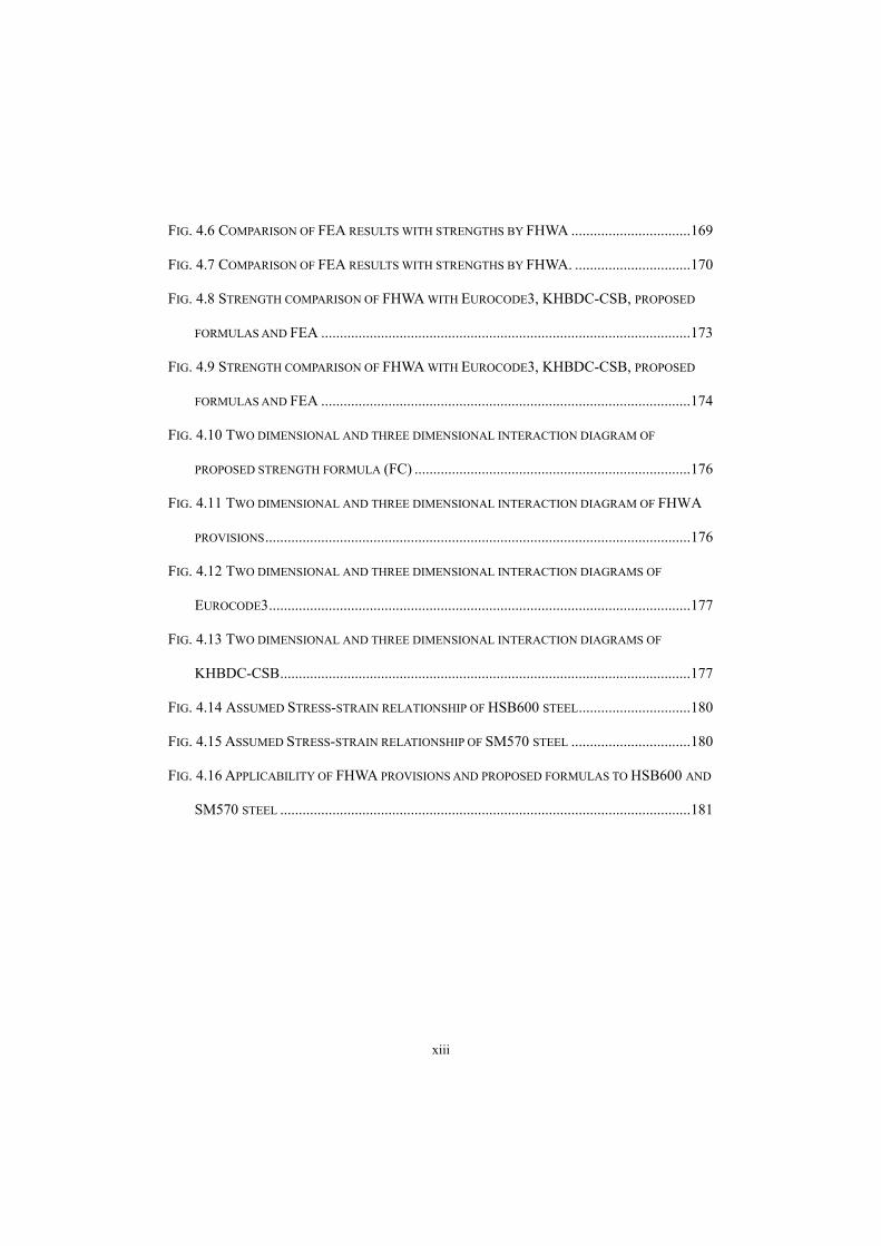
system can support the failure load (Gere, 2001). Fig. 2.1 shows a certain load-

displacement curve for a thin stiffened flange. Theoretically, point C is the ulti-

mate strength. Sometimes point A can be used as a strength limit when considering

serviceability in the context of design philosophy. If the small deformation as-

sumption is used, then point B, which has an average effective plastic strain equal

to the yield strain, will be the strain limit as suggested by Hill (1998). Point B has

a possibility to occur prior to point C. In this study, point C is used as the ultimate

strength and point B is considered a constraint term.

13

0

0.2

0.4

0.6

0.8

1

0 2 4 6 8 10 12

td=8mm, L=3587mm

Nor

mal

ized

Str

engt

h (F

u/F

y)

Displacement (mm)

AC

B

average of effective

plastic strain = y

Fig. 2.1 Load-displacement curve of stiffened thin flange

As explained in chapter 1, inelastic buckling modes of the stiffened flanges under

uni-axial compression are (1) plate-type (local) buckling, (2) positive column-type

(global) buckling, (3) negative column-type (global) buckling and (4) stiffener lo-

cal buckling. The stiffener local buckling is inherently prevented in a design step

due to the requirements that the ultimate compressive strength of stiffeners must be

greater than that of stiffened flanges. Thus, the ultimate compressive strength of

general stiffened flanges occurs through three behaviors. The plate-type buckling

is called plate-like behavior, and the positive or negative column-type buckling is

called column-like behavior in Eurocode3 (EN1993-1-5, 2004). As a result, the

inelastic buckling modes of the stiffened flanges can be defined as the two behav-

iors.

14

2.2 Theory of small deformation plasticity in stiffened flanges

In this section, a preliminary study is performed to determine the analysis level.

Then, the theories used in this study are described in detail.

(1) Preliminary study on stiffened flanges

To check the strain level of stiffened flanges at an ultimate state, a numerical

compression test is performed. Numerical models for the test are thin, intermedi-

ate and thick stiffened flanges, and these three models have the same longitudinal

(column) slenderness parameter (L/r). Initial geometric imperfection is consid-

ered as the positive column-type buckling mode and the maximum magnitude is set

at L/1000. In the case of residual stress, Fukumoto’s model, which has Fy in ten-

sion area and 0.25Fy in compression area, is used. To evaluate a state of whole

strain in the stiffened flanges, an average value of effective plastic strain on the

flange plating is used (Chen, 1988). If the effective plastic strain reaches the yield

strain, we can roughly consider the total strain as two times the yield strain (2εy).

Fig. 2.2 shows the load-displacement curves and an average of effective plastic

strain at ultimate states of the stiffened flanges. All cases show the average values

of effective plastic strain is less than the yield strain. According to Hill (1998),

small deformation limits are defined such that total strain is smaller than 2εy or

plastic strain is equal to elastic strain. Therefore, the above stiffened flanges with

U-ribs can be analyzed by the small strain theory.

15

0

0.2

0.4

0.6

0.8

1

0 2 4 6 8 10 12

Thin plate (td=6.8 L=5094)

Intermediate thick plate (td=12.7 L=4709)

Thick plate (td=29.6 L=3802)Ulti

mat

e C

ompr

essi

ve S

tren

gth(

Fu/

Fy)

Displacement (mm)

ep = 0.64y

ep = 0.57y

ep = 0.8y

Fig. 2.2 Average values of effective plastic strain at the ultimate states of stiff-ened flanges

In the small-deformation plastic theory, a boundary value problem always has

a unique solution when the yield function and plastic potential are identical (Hill,

1998). Some researchers showed this uniqueness mathematically (Khludnev et al.,

1997).

(2) Small deformation assumption on strain and stress

When a body is applied to external forces, the body goes into an equilibrium

state after deformation. Thus, equilibrium equations have to be defined at the

deformed geometry. However, if deformation is small, there is no difference be-

tween the undeformed and deformed geometry. Therefore, a strain can be ex-

pressed as a linear function of displacements, ignoring the high order term defined

16

in the Green strain as shown in Eq. (2.1).

X

u

X

uε

T

2

1(2.1)

where X denotes the undeformed geometry and ε is usually called the engineering

strain.

Different stresses can be defined based on the reference of geometry. The

following relations show the Cauchy stress tensor σ .

nσQ

t

S

lim0S

(2.2)

σ is derived from the definition of surface traction t . S , Q , and n are an

infinitesimal area defined in deformed geometry, the force on it and the unit normal

vector on the area, respectively. σ is often called true stress in commercial pack-

age programs because σ is defined in the deformed geometry for both the force

and the area. However, we can use the stress at an undeformed geometry due to

small deformation assumption. In this study, engineering strain and Chauchy

stress at undeformed geometry are used.

(3) General in elastoplasticity

Generally, strain energy density exists in the property of elasticity. Stress is

uniquely determined by differentiating the density function with respect to the

17

strain because the material has one-to-one mapping between the stress and strain.

This property is called path-independent. Thus, regardless of the loading paths,

stress exists and has only one value for corresponding to a certain strain. From

this property, if a load is applied to a structure and removed, then the structure goes

back to the initial state.

In contrast to elasticity, some materials show permanent deformation if a load

over a certain threshold value is applied and removed. This property is called

plasticity. Unlike an elastic material, a one-to-one relation between stress and

strain does not exist. In other words, for a certain strain , there are infinite

stresses corresponding to the strain because there are so many load paths to pro-

duce the strain . Thus, this property is called path-dependent. Most of the

materials are initially elastic and become plastic if an applied load gradually in-

creases. We call this property elastoplasticity.

The elastoplastic problem belongs to the material nonlinear problem. As

mentioned, there exists a unique solution only for the small deformation plastic

problem in a special case. On the contrary, a unique solution for the large defor-

mation plastic problem is not known yet. Therefore, the limit of a solution area

that we can guarantee is the small deformation plastic problem. In this study, all

descriptions will be focused on the small deformation elastoplastic theory.

The non-linearity of elastoplasticity comes from nonlinearity of the stress and

strain relationship. Unlike the elastic problem, the stress and strain relationship

cannot be defined as a total form in an elastoplastic problem. Instead, the rela-

18

tionship is defined as a rate form

)( ef (2.3)

where , e and f denote a stress rate, elastic strain rate and constitutive rela-

tionship, respectively. The rate form can be understood as an incremental form in

a static analysis. Under the small deformation assumption, a total strain can

be additively decomposed into sum of an elastic strain e and a plastic strain p

as following.

pe pe pe (2.4)

where ‘dot’ and are the rate and increment of the strain. If the elastic strain is

determined, stress can be calculated from the equation because only the elastic

strain contributes to the stress. Then, the plastic strain is calculated by subtracting

the elastic strain from the total strain. The plastic strain does not contribute to an

increase of the stress, but evolve the elastic domain. In an elastoplastic analysis,

the most important job is to separate the elastic and plastic strains from the total

strain. We need three essential components to complete the job, which are a yield

criterion, a hardening rule and a flow rule. From these, stress will be updated

with numerical methodology.

19

(4) von Mises yield criterion

A plastic behavior starts from material yielding. Yielding of a one-

dimensional (1D) element such as a truss can easily be defined from the stress-

strain curve (uniaxial tension test result). However, in the case of a multi-

dimensional element such as a shell, there exist infinite combinations of stresses

for material yielding. Thus, we need some scalar measure to define the yielding

in a multi-dimensional case. There are two well-known scalar measures for the

material yielding. One is the maximum shear stress by Tresca and the other is the

distortional strain energy density by von Mises. In this study, the distortional

strain energy density will be used for the yielding measure.

If a body is deformed by an external load, then two types of deformation can

occur. One deformation is dilatational deformation and the second is distortional

deformation. The former is related to the volumetric strain and the latter is related

to the deviatoric strain. Plastic deformation is only concerned with the deviatoric

strain. The distortional energy density can be defined as

sses :4

1:

2

1

devU (2.5)

Eq. (2.5) denotes the deviatoric part of the strain energy density. The last relation

uses es 2 . Where , s , e mean Lame’s constant, deviatoric stress and

strain tensor, respectively. The deviatoric stress and strain tensor are calculated as

20

1σs m , volm 3

1)(

3

1332211

1εe m , volm 3

1)(

3

1332211

(2.6)

Subscript m and vol denote mean (average) and volume, 1 is the second order

unit tensor. If devU equal to the distortion energy density at material yielding

from the uni-axial tension test 2)6/(1 yf , then we can define the yielding measure

as

ye f ss :2

3 (2.7)

where e is called the effective stress. The effective plastic strain is defined as

ppppppe εεee :3

2:

3

2(2.8)

pe is the plastic part of the deviatoric stain. The last relationship in Eq. (2.7) can

be rewritten as the expression.

03

2

3

2:)( yyvon ffF sssσ (2.9)

Eq. (2.9) is called von Mises yield criterion. If ye f or 0)( σvonF , then the

21

material is under a yielding state. However, if ye f or 0)( σvonF , the mate-

rial is under an elastic state. ye f or 0)( σvonF is fundamentally impossi-

ble. The effective stress of Eq. (2.7) can be written in terms of the second devia-

toric stress invariant 2J .

2222222 )()()(

6

1:

2

1zxyzxyxzzyyxJ ss (2.10)

As a results, von Mises yield theory is called 2J plasticity.

(5) Isotropic hardening

If the yield stress of a material is given from the uni-axial tension test, the

yield criterion can be determined by the von Mises theory. Additional considera-

tions are required for an increase of the yield stress itself, which is called strain-

hardening. Generally, there exist two well-known strain hardening models. The

first is the isotropic hardening model and the second is the kinematic hardening

model as shown in Fig. 2.3. The isotropic hardening model widens the boundary

of yield criterion itself due to accumulation of the plastic strain. However, the

kinematic hardening model moves the center of the yield criterion instead of

changing the criterion size. In the next section, we describe the linear isotropic

hardening model used in this study.

In the isotropic hardening model, the yield stress increases according to the ac-

22

cumulated effective plastic strain as

pyy Heff 0(2.11)

where 0yf is the initial yield stress and H is the plastic modulus from the stress-

strain curve.

peH

(2.12)

If linear isotropic hardening is assumed, H becomes constant and has a relation-

ship with the elastic modulus E and tangent modulus tE .

t

t

EE

EEH

(2.13)

To reflect the strain-hardening effect, von Mises yield criterion in Eq. (2.9) can be

modified as

0)(3

2),(),( ppvonvon eeFF ssσ (2.14)

where )( pe is the evolved yield stress and determined by the accumulated ef-

fective plastic strain. Geometric interpretation of )(3/2 pek is the radius of the

yield circle in the space of the deviatoric stress.

23

Fig. 2.3 Two different types of hardening model

(6) Associative flow rule

The flow rule explains how the plastic strain increment evolves. In metal

plasticity, the flow rule is defined as (Crisfield, 1997)

mε p (2.15)

where and m are the magnitude and direction of plastic flow, respectively.

When there is plastic potential g , the plastic strain increment evolves in the nor-

mal direction to the plastic potential as

σ

σε

),( g

p (2.16)

where is the hardening variable. If the plastic potential is equal to the yield

function as defined by Eq. (2.9), then we say that the plastic model obey the asso-

ciative flow rule. In terms of the uniqueness, only small deformation plasticity

Evolution of the yield surfaceInitial yield surface, fy

0

Evolved yield surface, fy

Initial yield surface

Evolved yield surface

Evolution of the yield surface

(a) Isotropic hardening (b) Kinematic hardening

24

with associative flow rule guarantees a unique solution. Eq. (2.16) with respect to

yield function is expressed as

Ns

s

s

sε

),( pvonp

eF(2.17)

where and N denote the non-negative plastic consistency parameter and a unit

deviatoric tensor which is normal to the yield function, respectively. Eq. (2.17)

shows that the plastic strain increases in a normal direction to the yield surface and

the magnitude is equal to . If is equal to zero, material is under the elastic

state. However, if is greater than zero, then the material becomes a plastic

state. If stress on the yield criterion ( 0vonF ) is changed to another state, then,

there exist three different cases.

(a) 0vonF , 0 plastic loading

(b) 0vonF , 0 neutral loading

(c) 0vonF , 0 elastic unloading

(2.18)

Especially, case (a) is called a consistent condition and can be expressed as

0:

:

pp

vonvon

pp

vonvonvon

ee

FF

ee

FFF

ss

σσ

(2.19)

25

Using Eq. (2.14) and Eq. (2.17), can be calculated as

03

2:2:2

3

2: HeH p NNεNsN

H3

22

:2

εN (2.20)

Where is Lame’s constant, s and pe are the deviatoric stress rate and effec-

tive plastic strain rate, respectively.

Nes 22 eNεN ::

3

2

3

2:

3

2:

3

2 ppppppe εεεee

(2.21)

For the reason that plastic deformation only occurs in deviatoric parts, effective

plastic strain rate is the same as the plastic strain rate (Kim, 2014).

(7) Methodology for updating stress

From the von Mises yield criterion, and isotropic hardening and associative

flow rule, a method how to update a stress by incremental loading is to integrate

the rate form of constitutive relations and plastic variables. Actually, the consti-

tutive relations of many metals at low temperatures relative to their melting tem-

perature and low strain rates do not depend on the rate of deformation (ABAQUS

2011). As this reason, integration of the rate form can be replaced by integration

26

of the incremental form.

The increment of stress is only related to the increment of the elastic strain.

We know the total strain increment but we do not know how much of the elastic

increment. Thus, we have to separate the plastic strain increment from the total

strain increment. The total strain increment can be decomposed into volumetric

and deviatoric increments. We aim to find the plastic strain increment in a devia-

toric space for determining why the plastic deformation only occurs in the deviato-

ric increment. Thus, the radial return mapping method is used in this study.

This method is a special form of backward-Euler procedure in which iterations are

not required for the von Mises yield criterion with linear isotropic hardening. The

return mapping method consists of two parts. The first part is elastic prediction

and the second part is plastic correction. From the given stress and plastic vari-

able in time nt , updated values in 1nt are expressed as

correctionplasticpredictionelastic

1 22 Ness μμnn

correctionplasticpredictionelastic

1

3

2 p

np

n ee(2.22)

If stress from the elastic prediction reside in the elastic domain, the stress and plas-

tic variable are directly updated and do not require a correction. However, in the

opposite case, a plastic correction is needed and N and have to be deter-

mined.

27

Fig. 2.4 Radial return mapping method for isotropic hardening

Fig. 2.4 shows that the direction of return mapping corresponds with radial direc-

tion N . Therefore, only is unknown. From the condition that the yield

function by the updated stress and plastic variable have to satisfy the evolved yield

criterion, can be determined as

0)(3

2),( 11111

pnn

pnn

vonn eeF ss (2.23)

H

epntr

3

22

)(3

2

s(2.24)

N2e2

)( pne

)( 1p

n e

σtr

σn

σ1n

01 von

n F

0vonnF

28

where ess μntr 2 is applied. The stress and stress increment can be calcu-

lated from Eqs. (2.22), (2.23) and (2.24).

σσσ nn 1

NεDσ 2:(2.25)

(8) Consistent tangent modular tensor

In material non-linearity, the structural tangent stiffness is defined as

dVBDBΚ :: TT (2.26)

Where B and TD are the strain-displacement tensor and the classical tangent

modular tensor, respectively. In continuum elastoplasticity, TD is defined as the

relationship between total stress and strain rate.

εDσ :T (2.27)

Since the stress rate is only related to the elastic strain rate, we can apply the fol-

lowing equation as

)(:)(:: NεDεεDεDσ pe (2.28)

Pre-multiplying the upper equation by N and then substituting the equation into a

consistent condition Eq. (2.19), we can express Eq. (2.27) as

29

εDεNDN

NDNDDσ ::

3

2::

):():(T

H

εDσ :T

(2.29)

In an overall equilibrium equation, the classical tangent modular tensor in Eq.

(2.29) does not guarantee a quadratic convergence in a Newton-Raphson type

scheme. Actually, TD is the tangent stiffness between the stress and strain rate,

However, if we use TD as the relation between the stress and strain increment,

then there is inconsistency. To overcome the inconsistency, Simo and Taylor

(1985) derived a tangent modular tensor, which is fully consistent with the back-

ward-Euler integration method. The tangent modular tensor can be derived from

the stress-strain increment relation. The general form and differentiation of Eq.

(2.25) can be rewritten as

NDεDσ :: (2.30)

σσ

NDNDεDσ ::::

(2.31)

Summarizing the expression with respect to σ ,

)(:)(:::1

NεQNεDσ

NDIσ

(2.32)

30

where, Dσ

NDIQ ::

1

Pre-multiplying the upper equation by N and substituting into the consistent con-

dition in Eq. (2.19), the consistent tangent modular tensor CTD can be derived as

εDεNQN

NQNQQσ ::

3

2::

):():(CT

H(2.33)

Compared with the classical tangent modular tensor TD , Q is replaced by D in

order to consider the change of direction N because is not infinitesimal. In

this study, modified Riks method with consistent tangent modular tensor will be

used.

(9) Finite rotation with Green-Naghdi objective stress rate

Under the small deformation assumption, finite rotations are considered for

analyses of the ultimate compressive strengths of stiffened flanges in this study.

In order to implement the finite rotations, we need some quantities called the ‘ob-

jective rate’, which is invariant under rigid body rotations. The Cauchy stress we

used is not invariant under the rigid body motions. Depending on the degree of

approximation, the objective rate for Cauchy stress σ can be representatively clas-

sified into three types as

31

Truesdell rate:

σLσLLσσσ )(TR trT (2.34)

Green-Naghdi rate:

σΩΩσσσ GN (2.35)

Jaumann rate:

σWWσσσ J (2.36)

In the Truesdell rate, tr is the trace operation and L is the spatial gradient of mate-

rial velocity with respect to the current configuration (De Borst et al., 2012).

TFFx

X

X

u

x

vL

(2.37)

where X and x denote undeformed and deformed configuration, respectively. The

Green-Naghdi rate is the approximated version of the Truesdell rate because the

Green-Naghdi rate uses the relation

TRRΩ (2.38)

RRUF (2.39)

where Ω is the rate of rigid body rotation at a material point, and R and U are

rigid body rotation and stretch in the polar decomposition of the deformation gradi-

ent F , respectively. In the Jaumann rate, W is the spin tensor expressed as

32

T

TT

T

RR

RUUUURRR

LLW

)(2

1

)(2

1

11 (2.40)

Since TRRW , the Jaumann rate is the approximated version of the Green-

Naghdi rate. For the shell element, Green-Naghdi rate GNσ (ABAQUS 2011) is

typically used. With the help of the Green-Naghdi stress rate, the constitutive

relation in Eq. (2.33) is still applicable to finite rotation.

εDσ :CTGN

εDσ :CTGN (2.41)

However, McMeeking et al. (1975) showed that incremental constitutive relation

from the rate form only achieves objectivity under a vanishingly small time step.

As a result, this condition may lead to excessive error accumulation in practice

because Eq. (2.39) is not accurate. To overcome excessive error accumulation,

Hughes et al (1980) proposed the midpoint incremental approach for time integra-

tion using the equation

uxx

2

1

t

)( 21 n/n

uxx 2

121 n/n

(2.42)

33

Assuming 1n as current step, nx and 21/nx are previous and mid-point con-

figuration, respectively. u is the velocity of material point. In order to calculate

the strain increment ε , derivative of Eq. (2.42) with respect to mid-point con-

figuration have to be carried out.

1

1

1

21

2121

2

11

2

11

LL

x

u

x

u

x

x

x

u

x

x

x

u

x

u

nn

n

/n

n/n

n

n/n

(2.43)

In finite element formulation, x

u

can be expressed in terms of shape function.

dx

N

x

u

I

(2.44)

ξ

NJ

ξ

N

x

ξ

x

N

I1

II

(2.45)

Where IN and d denote the displacement shape function and nodal displace-

ment increment, x and ξ are material coordinates and its corresponding coordi-

nate in the parent element. Especially, J is the Jacobian matrix that relates these

two coordinates. From the upper relation, the strain increments at the mid-point

are expressed as

34

T

T

LLLLε2

11

2

11

2

11

(2.46)

The stress at the previous load step is also transformed to the unrotated configura-

tion as

T/nn/nn 2121 RσRσ (2.47)

1212121

/n/n/n UFR

)(2

121 uIF n/n

2/1212121 )( /n

T/n/n FFU

(2.48)

The rotation 21/nR is obtained from the polar decomposition of 21/nF . Eqs.

(2.42), (2.43), (2.44), (2.45), (2.46), (2.47) and (2.48) shows the requirement of the

updated Lagrangian formulation. However, the strain is small because finite rota-

tions have to be described by deformed geometry.

(10) Updated Lagrangian formulation for large rotation.

A Large rotation with a small strain is similarly treated with a large deforma-

tion problem. To solve this problem, we have to use the updated Lagrangian for-

mulation because a plastic variable is directly related with Cauchy stress. If we

have the solution at load step n , then a new solution can be determined from the

principle of virtual work at the current load step 1n as (Kim, 2014).

35

0ddΩdΩ:)(

WWW

1111

111

snnn

TTn

next

nint

n

Tubuσuε

(2.49)

Since the above equation is a nonlinear function of displacement, the equation has

to be solved with an iterative scheme. Linearization of the first term on the right

side leads to

dΩ:

dΩ:)(W

11

11

1

1

nn

nnint

n

n

σu

σuε

(2.50)

Using the domain change, Eq. (2.50) can be rewritten at the undeformed configu-

ration.

dΩ]:)(:)(:))([(

dΩ:)(W

11

011

011

0

11

01

0

0

JJJ

J

nnn

nnint

σuFσuFσFu

σFu

(2.51)

where F and )( 1 F are increments of the deformation gradient and its inverse,

and J is an increment of the Jacobian matrix. These terms are calculated as

uX

u

X

uxF

00

)(

uFuFFF

111

011)( n

)()det( uF divJJ

(2.52)

Substituting Eq. (2.52) into Eq. (2.51), each term in Eq. (2.51) is calculated as

36

J

JJT

nnn

nnnn

uσu

σuuσFu

111

11111

0

:

::)(

(2.53)

JJ Tnn

Tnn )(::)( 11GN

111

0 RRσσRRσuσuF

(2.54)

JdivJ nn )(::)( 111

0 uσuσuF (2.55)

Hence, we shall omit the subscript 1n when referring to the current )1( n th

stress. After combining the upper three terms, we can rewrite Eq. (2.49) as

dΩ])()([:W 1GN

11

1

Tn

TTn

nint div

n

uσuσRRσσRRσu

(2.56)

From the assumption of Eq. (2.39), TRR can be expressed in terms of the spatial

gradient of displacement increment x

u

. After summarizing the integrand with

respect to x

u

, we have

dΩ)(:)(:)(:W1

111SCCT11

nn

Tnnn

nint sym uuσuDDu (2.57)

The first and second terms in the integrand are tangent stiffness and initial stiffness,

respectively. Especially SCD in the first term is the spatial constitutive tensor

representing the rotational effect of Cauchy stress.

37

)( jkiljlikklijijklSCD (2.58)

Finally, Eqs. (2.49), (2.50) and (2.55) provide the incremental equation as

dΩ:ddΩ

dΩ)(:)(:)(:

111

1

1

111SCCT1

σuTubu

uuσuDDu

nsnn

n

nTT

nT

nnn sym

(2.59)

After incremental displacement is converged at the current load step, the return

mapping procedure is conducted for the next stress and plastic variable.

(11) Finite element procedure for small-deformation plasticity with large rotation

The computational steps are:

Step 1. Compute the strain increment at 21/n

)( 1/2n uε sym (2.60)

Step 2. Compute the rotation matrix at 21/n using Eq. (2.48)

1212121

/n/n/n UFR (2.61)

Step 3. Rotate the stress to unrotated configuration.

T/n/n 21n21n RσRσ (2.62)

38

Step 4. Do the return mapping procedure with nσ

Step 5. Compute the internal force

n

ii

T W1

1nint ][ JσBq (2.63)

Step 6. Compute the tangent stiffness

i

n

i

T W

1

SCCTTan ]])[[]([][][ JBDDBK (2.64)

Step 7. Compute the initial stiffness ][ IniK

More details in this term are explained in ABAQUS manual (2011).

Step 8. Compute the incremental displacement

d][ intext1kIniTan qqKK (2.65)

Step 9. Update displacement

1kk1n

1k1n

ddd

1kk1k ddd (2.66)

If the residual force is not zero, the upper procedures are repeated until the dis-

placement increment is converged. Then, the next load step starts.

39

(12) Moment amplification by axial force

Under the small deformation assumption, moment amplifications by an axial

force are also considered. Although only in-plane compressive forces are applied

to the stiffened flanges with U-ribs, out-of plane displacements can significantly

occur due to the initial geometric imperfections and the redistribution effect of the

residual stresses. In this case, additional bending moments by the axial force are

definitely unavoidable. To consider this effect, the Nlgeom option in ABAQUS is

used. To verify the Nlgeom option, unstiffened flanges (0.2m1m0.01m) are

modeled and analyzed. The unstiffened flanges mimics a certain analytic beam-

column models, which is under the simply supported condition, an uniformly dis-

tributed load (pressure) and an axial force. The uniformly distributed load and the

axial force are summarized in Table. 2.1. For equivalent comparison between the

analytic beam-column and the unstiffened flanges, Poisson ratio is set at zero.

Numerical solutions with respect to on/off Nlgeom option are compared to

analytic solutions in Table 2.1 and Fig. 2.5. The results show that the Nlgeom

option considers only the moment amplification by the axial force under the small

deformation problem.

40

(a)

(b)

(c)

Fig. 2.5 Verification tests for the Nlgeom option in ABAQUS: (a) Unstiffenedflanges with simply support, uniformly distributed load and axial force (b) the ver-tical displacements by Nlgeom off and (c) the vertical displacements by Nlgeom on

41

Table 2.1 Verification of Nlgeom options using unstiffened flange

Axial force Distributed load L E I P/Pcr Max uz

Nlgeom off 7.813E-04

Nlgeom on41.115kN/m 1kN/m2 1m 200GPa 1.667E-08 0.25

1.042E-03

Analytic solution

Ignoring Moment amplification by axial force : 7.813E-04

Considering Moment amplification by axial force : 1.043E-03

(13) Modified Riks method for ultimate compressive strength

As shown in Fig. 2.1, we need to find the equilibrium path for the ultimate

compressive strength of the stiffened flange. A classical force method such as the

Newton-Raphson method cannot be used when structural instability occurs. In

this study, modified Riks method overcoming the limitation of the Newton-

Raphson method is used.

To evaluate the ultimate strength, we have to trace the nonlinear equilibrium

paths represented by the load-displacement curve and catch the upper limit point.

If the Newton-Raphson method is used, then it fails in the vicinity of a limit point

because the tangent stiffness matrix becomes singular. Thus, we need alternative

methods that enable the solution to path a limit point. In this regard, a type of arc-

length method is suitable, which was originally proposed by Riks (1972, 1979) and

Wempner (1971), and modified in other studies (Schweizerhof et al., 1986; Forde

et al., 1987). The main idea of these methods is to find an intersection point from

an equilibrium curve and given arc-length. Mathematically, arc-length has the

meaning of a constraint. Previously, Riks and Wempner used linear and fixed

42

constraints in the current increment. However, these constraints occasionally

failed to turn a limit point. Thus, Crisfield et al. (1981) proposed a spherical con-

straint, even though this type of constraint was cumbersome due to the choice of

root for a quadratic problem. Ramm (1981, 1982) converted Riks’ constraint into

a changeable one at each iteration step using a secant line of an equilibrium curve.

Fried (1984) modified Riks-Wempner and/or Ramm constraint more efficiently

using orthogonal trajectory. He ensured that the iterative change of linear con-

straint is orthogonal to a tangential line of equilibrium curve at each iteration step.

In this study, modified Riks method proposed by Fried is used. To trace the

nonlinear equilibrium curve by modified Riks method, we need the prediction-

correction method at each increment. Fig. 2.7 geometrically shows modified Riks

method. First, we obtain an initial guess and set ),( 11 ua from the latest con-

verged equilibrium set ),( 00 uo . Next, the set has to be corrected along the

a → b→ c→ ··· path until the equilibrium condition is satisfied exactly. Speci-

fically for an unknown variable, the equilibrium equation is written as

0)(),( extint ququR (2.67)

where intq denotes an internal forces vector, which is a function of displacement,

u and extq are a constant external loading vector controlled by a scalar load pro-

portionality factor , and R is the unbalanced force of the two quantities.

At the previous converged equilibrium set ),( 00 u , Taylor’s expansion of the

43

equilibrium equation can be written as

0)()( 000

00

Ruu

u

RR

uu

→ 0)()( 0000 quuKR

(2.68)

where

0T0

0

KKu

R

uu

(2.69)

qqR

ext

0 (2.70)

The first derivative term is a tangent stiffness matrix and the second derivative is

an external force vector.

For the initial prediction step, we have to move the previous equilibrium set

),( 00 u into a current initial guess ),( 11 u using the constraint equation.

22010101 )()()( rT uuuu

→ 20000 rT uu

(2.71)

where r is a step size called the radius of arc-length. Combining Eq. (2.68) and

Eq. (2.71), we can produce an initial guess ),( 11 u .

44

qKKq 10

10

011

T

r

qKuu 10001

(2.72)

Next, we need a correction step by using the Newton-Raphson method because

an initial guess is not on the equilibrium curve. To move ),( 11 ua into

),( 22 ub as shown in Fig. 2.7, we exploit the two conditions. First,

),( 22 ub lies on the Taylor expansion of R at ),( 111 e us . Second, the

correction vector from a to b should be orthogonal to the last tangent rather than

the tangent at the beginning of the increment. This is called orthogonal trajectory.

If the direction of correction vector is not changed, then it becomes Riks and

Wempner method as seen in Fig. 2.6.

For the first condition, ),( uR linearized at ),( 111 e us lead to

0),()()(

)()(),(),(

11111

111111

111

uRquuK

Ruu

u

RuRuR

uu

eee (2.73)

Substituting ),( 22 ub into Eq. (2.73), 1u is determined as

01111 RquK

→ )( 111

11 RqKu (2.74)

For the second condition, the orthogonal relation is defined as

45

01010 uu T (2.75)

Using Eq. (2.72), the linear constraint that relates 1 to 1u is expressed by

1111

110

01 uαuqKu

u TT

T

(2.76)

where vector 1α determines the direction of the correction vector. Substituting

Eq. (2.74) into Eq. (2.76), 1 is determined as

qKα

RKα1

1

11

11 1

T

T

(2.77)

From Eq. (2.74) and Eq. (2.77), we can correct the initial guess as

112 uuu

112 (2.78)

If ),( 22 u is not on the equilibrium curve, then Eqs. (2.73), (2.74), (2.75), (2.76),

(2.77) and (2.78) proceed again until converged. Figs. 2.6 and 2.7 show the dif-

ference between Riks method and modified Riks method. Riks method uses a

fixed 1α for the correction vector until convergence. However, modified Riks

method with orthogonal trajectory changes its direction of the 21 αα

path as the correction step proceeds.

46

Fig. 2.6 Riks Method (Riks and Wempner)

Fig. 2.7 Modified Riks Method (Fried method)

),( 222 e ut

),( 33 uc

),( 111 e us

),( 00 uo

),( 22 ub

),( 11 ua

2e1e

u

0),( uRr

),( 222 e ut

),( 33 uc

),( 111 e us

),( 00 uo

),( 22 ub

),( 11 ua

2e1e

u

0),( uRr

47

2.3 Finite element modeling of stiffened flanges with U-ribs

In this section, stiffened flanges are modeled with finite elements by commercial

software ABAQUS (2011). The elements used in the stiffened flanges are based

on thin shell theory. Quadrilateral bilinear element S4R5 is used (Ellobody, 2014).

The element uses small strain assumption. The element has five degrees of free-

dom per node and one Gauss point for reduced integrations. The essential idea of

the S4R5 element is that the position of a point in the shell reference surface x and

the components of vector n, which is normal to the reference surface, are interpo-

lated independently. The kinematics of shell theory then consist of measuring the

membrane strain on the reference from the derivatives of x with respect to a posi-

tion on the surface and bending strain from the derivatives of n. The used strain

measures for this purpose are approximations to those of Koiter-Saders theory

(Budiansky and Saders, 1963). The transverse shear strains are added to the thin

shell element and measured by the changes in the projections of n onto tangents of

the shell’s reference surface. Although the transverse shear deformations are con-

sidered as penalty terms that enforce the constraint, the solution by this element

converges to the classical solution of the thin shell theory as thickness of the shell

diminishes.

According to previous research (Grondin et al., 1999), the yield strength is an

influential variable for the ultimate compressive strength of stiffened flanges.

Defining the exact yield point is very important. Hence, conventional steel such

48

as SM490Y having a clear yield point is used for the material model in this study.

In particular, yield and ultimate stress of SM490Y is similar to A 709M Grade

345W, which is designated by the American Society for Testing and Materials

(ASTM). The experimental material behaviors for stiffened flanges with U-ribs

are modeled as elasto-plasticity with a yield plateau and strain-hardening rate. All

parts of the stiffened flange and U-ribs are modeled with identical steel. Assumed

mechanical properties of the steel are summarized in Table 2.2 and Fig. 2.8 (Cho et

al. 2010, Manda et al. 2010). yF and uF are the yield and the ultimate stress of

the steel, and y , sh , u and shE denote the yield strain, starting point of

strain-hardening, the ultimate strain and strain-hardening rate, respectively.

Table 2.2 Mechanical properties of conventional steel

Type E (GPa) yF (MPa) uF (MPa) y sh u shE (GPa)

SM490Y 200 355 490 0.001775 0.021 0.0585 3.6

Fig. 2.8 Assumed Stress-strain relationship of conventional steel.

shEyF

uF

y ush

49

Fig. 2.9 Idealized boundary condition of stiffened flange with U-ribs

Fig. 2.9 shows the idealized boundary conditions in this study. On the top or

bottom flanges of a box girder, transverse diaphragms are designed to be

sufficiently stiff to ensure that they provide nodal lines, which act as simple

rotationally free supports to the ends of the stiffened flanges (Ziemian, 1998).

Considering the above condition, only Uy and Uz of the loaded edge, which are in-

plane displacements in terms of the diaphragm, are constrained on the both sides.

The unloaded edges of the stiffened flanges are in contact with the inner or outer

web of the box girder. We can assume that the webs are stiff in the in-plane

direction. However, considering the large compression in the X-direction, only

Uy is constrained. For the purpose of preventing instability and considering the

symmetric condition, the center node on the unloaded edges is constrained in the

Uy=0

Uy=Uz=0

Uy=Uz=0

Uy=0

Ux=0

Ux=0

Axial compression

50

X-direction (Ux=0).

A process of determining hypothetical models for the stiffened flange with U-

ribs is described as following. First, a typical U-rib model that has unchanged

shape, thickness and transverse spacing is assumed, because a type of U-ribs is not

various and a designer uses off the shelf U-ribs in the design practice. From the

fixed U-rib model, the number of required stiffeners is investigated based on the

elastic buckling strength of both thin and thick flanges. Second, the geometry of

the stiffened flanges is determined by considering the column and plate slenderness

parameters used in the FHWA-TS-80-205 report. In this study, only the thickness

and the longitudinal length of the flanges are varied along these two parameters.

Third, mesh tests are performed in the longitudinal and transverse directions in

sequence and quadratic convergence is confirmed.

Wide type U-rib stiffened flanges have to be able to reflect the wideness in its

behavior. This means that the stiffened flanges must be sufficiently wide to ex-

press both plate like behavior and column like behaviors. In addition, effects of

unloaded edges have to be ignored by sufficient stiffeners because we mimic only a

part of the top or bottom flange in the box girder. To determine the proper num-

ber of stiffeners, the elastic plate-type buckling strengths for thin flanges and elas-

tic column-type buckling strength for thick flanges are traced while increasing the

number of U-rib stiffeners. The dimensions of the U-rib stiffeners are summa-

rized in Fig. 2.10 and Table 2.3. The U-rib stiffener is the general model used in the

steel box-girder of In-cheon long-span cable stayed bridge (South Korea). The

51

thicknesses of thin and thick flanges are set at 40mm and 8mm, respectively.

Both longitudinal lengths are assumed at 3m.

Table 2.3 Geometry of U-rib (unit: mm).

U-rib type a w b h h′ R tr

4002408 400 400 250 240 251.4 40 8

Fig. 2.10 Geometry of hypothetical model

w w

R

td

h

b

h´

tr

L = 1.6m ~ 9.5m

B = 8m

Z

X

Y

a

52

Thin Plate (PLB Mode)

Thick Plate (CBN Mode)0

0.2

0.4

0.6

0.8

1

1.2

0 2 4 6 8 10 12 14

Number of Stiffeners

Nor

mal

ized

Ela

stic

Buc

klin

g st

ress

PCB = 1688MPa (Ns = 2)PPB = 347MPa (Ns = 2)

Converged

Fig 2.11 Required stiffeners in wide stiffened flanges

Fig. 2.11 shows the elastic buckling strengths normalized with respect to its

value for Ns=2. This reveals that the ten U-rib stiffeners are sufficient for the

wide stiffened flanges.

As explained in section 2.1, the behaviors of stiffened flanges under uni-axial

compression can be categorized into two major modes: the plate-like behavior and

the column-like behavior. In reference to the FHWA-TS-80-205 report, these two

behaviors can be explained by the plate slenderness parameter pl and the column

slenderness parameter col written in Eq. (2.79).

53

E

Ftw ydpl 9.1

/

E

Fwt ypl

d 9.1

/

r

L

E

Fycol

1

ycol F

ErL

(2.79)

where w is the net spacing between U-ribs(Fig. 2.10), dt is the thickness of

flange plate, L is the longitudinal length of a stiffened flange or transverse stiff-

ener spacing, and r is the radius of gyration of a strut. In this study, each

parameter is controlled by changing the flange plate thickness dt and longitudinal

length L of the stiffened flange. The overall width B of the stiffened flange is

determined as 8m when considering the number of stiffeners. As explained, the

geometric properties of U-rib stiffeners remain unchanged. The thickness and

length of the flange corresponding to slenderness parameters, which vary from 0.3

to 1.3, are summarized in Table 2.4. Thirty-six geometric models have been set

up. In these models, the range of thickness and the length of the stiffened flanges

are 6.823mm to 29.565mm and 1.629m to 9.46m, respectively. The thicknesses

of flange from P03 ~P09 series are on the general range used in the practical box-

girder, so the series are well proportioned section. They are designed referring the

In-cheon long-span cable stayed bridge. The P11 series and the P13 series in Ta-

ble 2.4 have non-practical thicknesses, but they are designed for additional studies

on the slender sections.

54

Table 2.4 Thickness and longitudinal length of hypothetical models according toslenderness parameter.

Model pl col dt (mm) L (mm)

C03 0.3 1629

C05 0.5 2716

C07 0.7 3802

C09 0.9 4888

C11 1.1 5975

P03-

C13

0.3

1.3

29.565

7061

C03 0.3 1878

C05 0.5 3131

C07 0.7 4383

C09 0.9 5635

C11 1.1 6887

P05-

C13

0.5

1.3

17.739

8140

C03 0.3 2018

C05 0.5 3364

C07 0.7 4709

C09 0.9 6055

C11 1.1 7400

P07-

C13

0.7

1.3

12.671

8746

C03 0.3 2101

C05 0.5 3502

C07 0.7 4903

C09 0.9 6304

C11 1.1 7705

P09-

C13

0.9

1.3

9.855

9106

C03 0.3 2152

C05 0.5 3587

C07 0.7 5022

C09 0.9 6457

C11 1.1 7891

P11-

C13

1.1

1.3

8.063

9326

C03 0.3 2183

C05 0.5 3639

C07 0.7 5094

C09 0.9 6549

C11 1.1 8005

P13-

C13

1.3

1.3

6.823

9460

55

A linear elastic compression test in a longitudinal direction is performed for

the P03-C03 model in order to determine the proper mesh size (Table 3). The

magnitude of the load is set at 300MPa. Longitudinal displacements at the center

of the loaded edge are traced to check convergence (Fig. 2.12). Since stiffened

flanges have different stiffness in the longitudinal and transverse directions, two-

way tests should be performed to easily confirm quadratic convergence. Thus,

mesh convergence is checked in the transverse direction after cutting the stiffened

flanges into equally spaced N divisions in the longitudinal direction. A test for

the meshes is shown in Fig. 2.13. The meshes are plotted as a purple line in Fig.

2.14. The results show that more than 13,120 meshes are sufficient for 32 longi-

tudinal divisions of the stiffened flanges. In this study, 18,000 meshes with forty

longitudinal divisions are used by the P03-C03 model in order to consider the area

of residual stress properly. One mesh size of this model is approximately

4cm4cm. This size is equally applied to the other models.

Fig. 2.12 Tracing point for longitudinal displacement in mesh convergence test

Tracing point

56

(a) Ntotal = 3520 (b) Ntotal = 6720

(c) Ntotal = 13120 (d) Ntotal = 27200

Fig. 2.13 The number of meshes cut into equally spaced 32 divisions in longi-tudinal direction

Fig 2.14 Longitudinal displacement versus the number of meshes

1010

10 10

N_long = 4N_long = 8N_long = 16N_long = 32N_long = 64Present study

1.114

1.115

1.116

1.117

1.118

1.119

1.120

102 103 104 105

Number of mesh (log scale)

Nod

al d

ispl

acem

ent (

mm

)

Nmesh = 18,000

57

2.4 Initial geometric imperfection

Inelastic buckling patterns of stiffened flanges are plate-type (local) buckling

(PLB) or positive column-type (global) buckling (CBP) or negative column-type

(global) buckling (CBN). Inspired by three failure modes, three types of initial

geometric imperfections are considered in this study. In order to implement each

initial imperfection type, the elastic buckling analyses (Szilard, 2004) by the Lanc-

zos method (Lanczos, 1950) is carried out for thin and thick plates under the in-

plane compression, respectively. More details of the Lanczos method are as fol-

lowing.

The eigenvalue problem for initial geometric imperfection can be written as

uKu (2.80)

where K is a symmetric nn matrix, and u and are eigenvectors and ei-

genvalues, respectively. The K matrix is Hermitian, which can be reduced into

a tridiagonal matrix by the Lanzcos algorithm.

mmm KQQT T (2.81)

mQ is an orthonormal basis of the Krylov subspace and mn matrix, and m is

the rank of Krylov subspace.

m21 qqqQ m (2.82)

58

mQ can be obtained by a similar Gram-Schmidt orthogonalization. mT is deter-

mined as (Lanczos 1950)

mm

m

1

1

32

221

11

m

T (2.83)

iTii Kqq , i

Tii Kqq 11 , i

Tii Kqq 1 (2.84)

By the QR factorization algorithm, Eq. (2.81) can be expressed as

)()( mmm QQKQQD T (2.85)

where Q is the multiple product of a local plane-rotation matrix. Components

of the diagonal matrix mD are eigenvalues and the column vectors of QQm are

eigenvectors. To calculate multiple roots, this method is expanded to a block

style (Grimes et al., 1994). Thus, the vectors iq in mQ are changed to a matrix

form. Generally, a block size is not greater than 7 in ABAQUS. A spectral

shifting scheme is also used for the numerical stability.

In order to implement the initial imperfection shapes, elastic buckling analyses

are conducted by the Lanczos method explained above paragraph. The reference

load is set to be in-plane axial compression (two-way unit pressure) in a longitudi-

59

nal direction. As a result, first eigenmodes are adopted for the initial geometric

imperfections (Bathe, 1996). As shown in Figs. 2.15(a) and 2.15(b), the plate-

type buckling mode (PLB) occurs in the thin flange, and the negative column-type

buckling mode (CBN) occurs in the thick flange. For an additional possible fail-

ure mode, the positive column-type buckling mode is also considered for initial

geometric imperfection as shown in Fig. 2.15(c). This mode is made with the

same magnitude and reverse direction of the negative column-type buckling shape.

In summary, three types of the initial geometric imperfection shapes are considered

for the ultimate strength analysis of the stiffened flanges. The magnitude of

maximum deflection (scale factor) max of the column-type buckling shapes is

assumed as 1000/L , which refers to the SSRC (Structural Stability Research

Council) column curve (Johnston, 1976). The assumed value is slightly more

conservative than 1500/L , which is in accordance with AISC (American Institute

of Steel Construction) specification (2005) and AASHTO (American Association

of State Highway and Transportation Officials) LRFD (load and resistance factor

design) bridge design specifications (2007) column curve (AASHTO LRFD 2007,

AISC 2005). For the plate-type buckling shape, the maximum magnitude of de-

flection is assumed as one hundred-twelfth of the plate width ( 120/w ), which

refers to Article 3.5 of the Bridge Welding Code (ANSI et al., 2002).

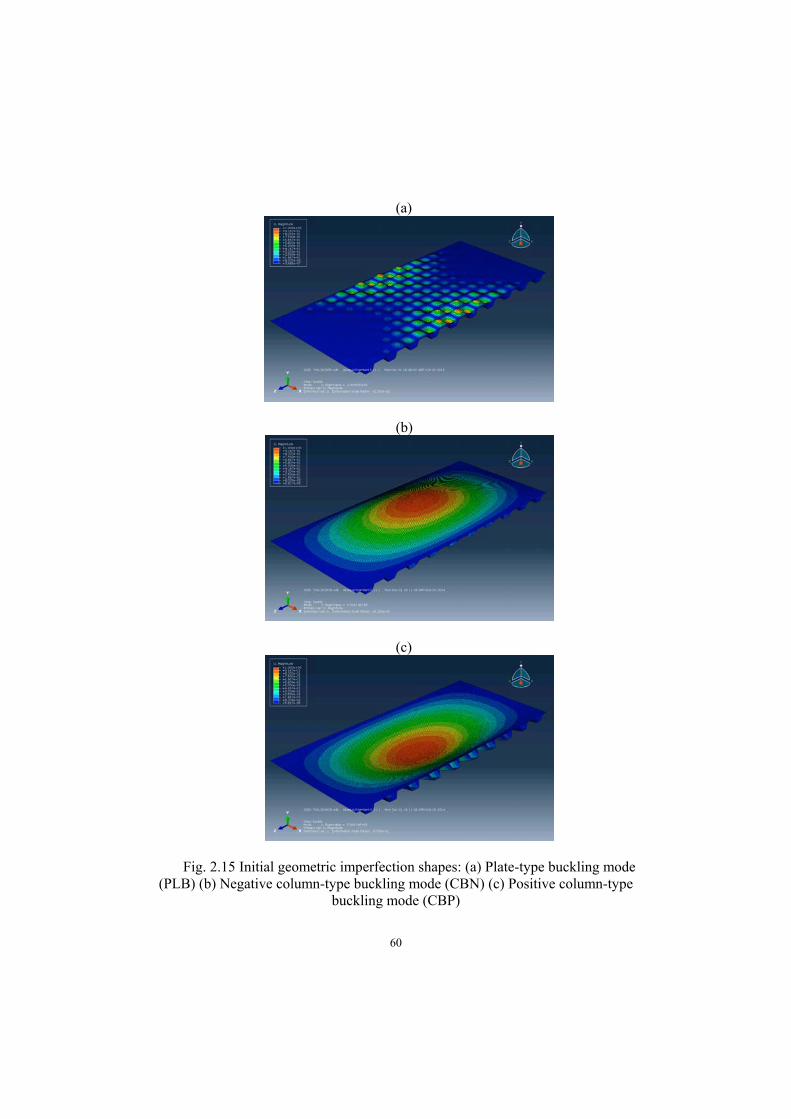
60

(a)

(b)

(c)

Fig. 2.15 Initial geometric imperfection shapes: (a) Plate-type buckling mode(PLB) (b) Negative column-type buckling mode (CBN) (c) Positive column-type

buckling mode (CBP)

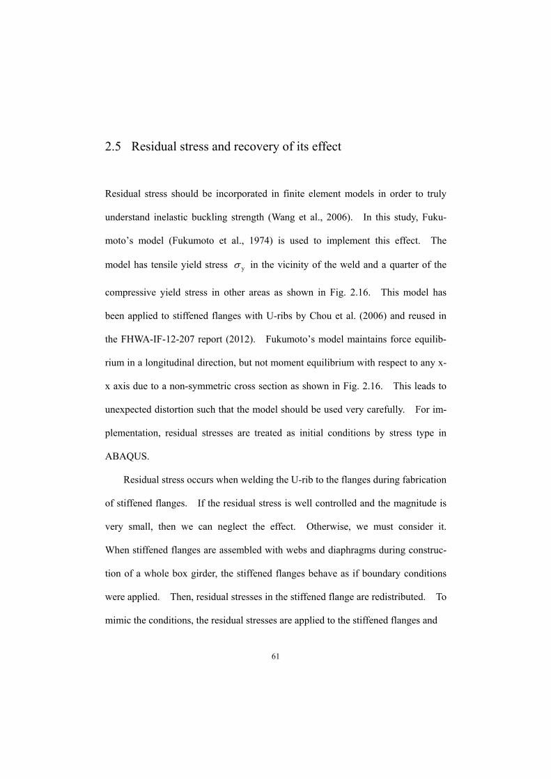
61

2.5 Residual stress and recovery of its effect

Residual stress should be incorporated in finite element models in order to truly

understand inelastic buckling strength (Wang et al., 2006). In this study, Fuku-

moto’s model (Fukumoto et al., 1974) is used to implement this effect. The

model has tensile yield stress y in the vicinity of the weld and a quarter of the

compressive yield stress in other areas as shown in Fig. 2.16. This model has

been applied to stiffened flanges with U-ribs by Chou et al. (2006) and reused in

the FHWA-IF-12-207 report (2012). Fukumoto’s model maintains force equilib-

rium in a longitudinal direction, but not moment equilibrium with respect to any x-

x axis due to a non-symmetric cross section as shown in Fig. 2.16. This leads to

unexpected distortion such that the model should be used very carefully. For im-

plementation, residual stresses are treated as initial conditions by stress type in

ABAQUS.

Residual stress occurs when welding the U-rib to the flanges during fabrication

of stiffened flanges. If the residual stress is well controlled and the magnitude is

very small, then we can neglect the effect. Otherwise, we must consider it.

When stiffened flanges are assembled with webs and diaphragms during construc-

tion of a whole box girder, the stiffened flanges behave as if boundary conditions

were applied. Then, residual stresses in the stiffened flange are redistributed. To

mimic the conditions, the residual stresses are applied to the stiffened flanges and

62

Fig. 2.16 Assumed residual stress distribution pattern

an iterative process is carried out at the empty load step to establish an equilibrium

state. This causes the magnitude and distribution of the initial imperfection in the

stiffened flanges to change. We can think of this case as the badly controlled

residual stresses during a fabrication. If we normally controlled residual stresses,

the distortion effects by the residual stresses have to be recovered but the residual

stresses are still maintained before beginning compression step.

Roman and Elwi (1987) controlled the distortion effects using an equivalent

temperature change for the stiffened cylinders. Equivalent temperature change

T is defined as

Eα

FT

T

rs (2.86)

where rsF is the residual stress, T and E are the coefficient of thermal expan-

sion and Young’s modulus, respectively. Similar procedures was performed in

many studies (Hu, 1993; Chen et al., 1993; Grondin et al., 1998). Especially, the

procedure was well developed and established by Sheikh et al. (2001) and Wang et

al. (2006). In Sheikh et al. (2001), a temperature change corresponding to the

+ +

- - -

Fy

0.25Fy + +

-

Fy0.25Fy

x x

63

negative values of desired residual stresses was applied to the initially perfect sys-

tem. Then, resulting displacements were added to the assumed initial geometric

imperfection to generate a new deformed and stress-free mesh. The temperature

change corresponding to the original desired residual stress was applied to the

newly generated model. After the equilibrium iteration at the dummy load step,

the model became a desired state. This method is based on the initially perfect

system. After a few years, Wang et al. (2006) developed this method based on

the initially imperfect system. As summarizing the updated method, negative

residual stress effect was applied to the model with assumed initial geometric im-

perfection. The resulting displacements were added on the assumed initial imper-

fection to generate a new stress-free mesh. Then, equilibrium iteration was per-

formed for a desired state. The latter method is a more complicated procedure

compared to the former method. In this study, we shall call the former as the

‘2001 method’ and the latter as the ‘2006 method’ for expressional convenience.

To evaluate the difference between the two methods, a preliminary study is

performed for the model used by sheikh (2001). The geometry and material prop-

erties are briefly described in Table 2.5 and Fig. 2.17.

64

Table 2.5. Geometry and material properties used in Sheikh et al.(2002).

Model bp Lu hw bf fyp fys tp tw tf

tp_PB 701.8 1264.4 150 135 420 420 16.1 11.5 12.4

Fig. 2.17 Cross section for preliminary study

Only a compression test without a bending moment by force control is per-

formed. The results are shown in Fig. 2.18(a), which reveals that there is no dif-

ference between the 2006 method and 2001 method. In addition, a comparative

study on the residual stress scheme is performed using stress-type initial conditions

instead of temperature change. The results are shown in Fig. 2.18(b). This ana-

lysis also shows that stress-type initial conditions and temperature change produce

an equivalent effect. In this study, the 2001 method by stress-type was used for

the convenience of implementation. In view of the fabrication procedure, the

deformation recovery method for residual stresses has a physical meaning in that

imperfect stiffened flanges are willfully fabricated in advance when we consider

the distortion by residual stress redistribution.

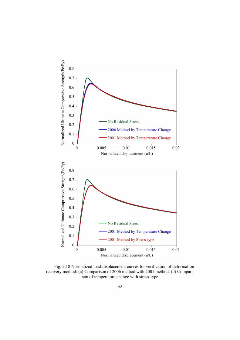
65

0

0.1

0.2

0.3

0.4

0.5

0.6

0.7

0.8

0 0.005 0.01 0.015 0.02

No Residual Stress

2006 Method by Temperature Change

2001 Method by Temperature Change

Nor

mal

ized

Ult

imat

e C

ompr

essi

ve S

tren

gth(

Pc/

Py)

Normalized displacement (u/L)

0

0.1

0.2

0.3

0.4

0.5

0.6

0.7

0.8

0 0.005 0.01 0.015 0.02

No Residual Stress

2001 Method by Temperature Change

2001 Method by Stress-type

Nor

mal

ized

Ult

imat

e C

ompr

essi

ve S

tren

gth(

Pc/

Py)

Normalized displacement (u/L)

Fig. 2.18 Normalized load-displacement curves for verification of deformationrecovery method: (a) Comparison of 2006 method with 2001 method. (b) Compari-

son of temperature change with stress-type

66

2.6 Force control and displacement control

If the bending moment caused by a dead load or a live load is applied to a box

girder, the top or bottom flanges become compressed states. If the diaphragms

(Fig. 2.20) are flexible (thin) enough, the longitudinal displacements of the loaded

edges will vary along the z-axis as shown in Fig. 2.19(a). However, if the dia-

phragms are stiff (thick), all parts of the loaded edge will have the same displace-

ment in the x-direction as shown in Fig. 2.19(b). The former example can be

analyzed by force control. The latter example can be analyzed by displacement

control. In addition, the ultimate compressive strengths by the force control and

the displacement control can be considered as lower and upper limits, respectively.

We can expect that actual strengths and behaviors of the stiffened flanges belong to

Fig. 2.19 Description of compression test by (a) Force control and (b) Dis-placement control

Displacement

Uniform Displacement

(b)

Displacement

Uniform Pressure

(a)

Flange edge

Flange edge

Flange edge

Flange edge

67

the intermediate range. In case of the force control, uniform pressures are im-

posed on the both sides of the U-rib and the flange edges using the shell edge load

option provided by ABAQUS. In case of the displacement control, uniform dis-

placements are imposed. The important thing is the boundary conditions (Fig.

2.9) in the force control and the displacement control are equivalent before loading

(axial compression).

To evaluate effects of diaphragms on the in-plane ultimate compressive

strength of stiffened flanges exactly, we must consider a ratio of the bending stiff-

ness bendingK of the diaphragm against the axial stiffness axialK of the stiffened

flange as shown in Fig. 2.20. Two stiffness terms can be defined as following.

Dbending BEIK )/( 3 , Paxial LEAK )/( (2.87)

If we think of the fixed end forces in the diaphragm as show in Fig. 2.21, bendingK

will denote the end reaction 3/12 BEI of the fixed end forces with respect to the

prescribed displacement 1 . Depending on boundary conditions, bendingK

can be generally expressed as 3/ BkEI . Thus, bendingK is set to be 3/ BEI in

this study. If we define an interpolation coefficient as a function of the stiff-

ness ratio,

)/( axialbending KKf (2.88)

68

the ultimate compressive strength uF can be determined by between the force

control strength ufF and the displacement control strength udF .

udufu FFF )1( (2.89)

If bendingK is much larger than axialK ( axialbending KK ), become one.

Conversely, if axialK is much larger than bendingK ( bendingaxial KK ), be-

come zero.

69

Fig. 2.20 Bending stiffness of diaphragm and axial stiffness of stiffened flangewith 10 Uribs

Fig. 2.21 Fixed end forces with respect to prescribed displacement in dia-phragm

Paxial LEAK )/(

Dbending BEIK )/( 3

B

L

tD

h

Stiffened flange with 10 Uribs

Diaphragm

Diaphragm

3

12

B

EI

3

12

B

EI

B

2

6

B

EI2

6

B

EI L

70

2.7 Modeling of diaphragms

In order to construct the bending stiffness of the diaphragms, the diaphragms are

modeled with finite elements. Fig. 2.22 and 2.23 shows the modeling of the dia-

phragms in this study. The boundary conditions in Fig. 2.9 are equivalently ap-

plied to the stiffened flange. The diaphragms are modeled with beam elements.

The stiffened flange and the beam elements are tied by rigid links. The flexural

rigidities and the torsional rigidity of the beam elements are defined as following.

12

3t

yy

EhDEI , xxEI , 0GJ (2.90)

As the loaded edges of the stiffened flange are simply support condition Uy=Uz=0,

xxEI of the diaphragm is the same as infinity. In addition, the loaded edges of the

stiffened flange are rotationally free support, GJ is set at zero. Thus, only

yyEI is working on the stiffened flange. If 0yyEI , we can mimic the force

control exactly. If yyEI , we can expect the effect of the displacement con-

trol. However, it is not possible to mimic the displacement control wholly, becau-

se a serrated shape of the diaphragms in Fig. 2.22 can not hold the all parts of the

cross-section of the stiffened flange. If a rectangular diaphragm is used, then we

can mimic the effect of the displacement control exactly as yyEI is increased to

infinity.

71

Fig. 2.22 Modeling of diaphragms using beam element and rigid link

h

tD

B

Uy=Uz=0

Uy=0

Ux=0

Uy=0

Ux=0

Uy=Uz=0

Stiffened flange with 10 U-ribs

Diaphragm

Beam element

Rigid link

Stiffened flange

72

Fig. 2.23 Modeling of stiffened flange and diaphragms in ABAQUS

If we use the shell elements (defined in section 2.3) for modeling of the dia-

phragms, the diaphragms will be directly tied to the stiffened flange. Then, the

connection becomes rigid joints. In this case, rotational constraints occur at the

loaded edges. Thus, this condition can not satisfy the rotationally free support

that the diaphragm has to provide it for the stiffened flanges. When the bending

stiffness of the diaphragm is considered, the only way to impose the same

boundary conditions on the force control and the displacement control is to model

the diaphragms as the beam elements and the rigid links.

In this study, the thickness of the diaphragm are set at 10mm, 20mm and

40mm considering the practical thickness, which is lesser than 30mm.

73

2.8 Proposed method for evaluation of ultimate compressive

strength of stiffened flanges with U-ribs

In this section, how to determine the ultimate compressive strength of the stiffened

flanges defined in Table 2.4 is described. For one stiffened flange, the elastic

buckling analysis and the inelastic buckling analyses are conducted in this study.

The prior is an eigen-value problem for an initially perfect stiffened flange, so pro-

cedure is very simple and no more consideration is required. However, the latter

is the load-deflection problem for an imperfect stiffened flange, so we have to con-

sider the several imperfect conditions.

For the inelastic buckling analyses, three cases of initial geometric imperfec-

tions are considered. These cases are positive column-type buckling, negative

column-type buckling and plate-type buckling. In addition, three cases of residual

stresses are considered. The first case is ‘not-considered’. The second case is

‘simply-considered’, which only does the redistribution. The third case is ‘con-

sidered with recovery’ which recovers the distortion effect. Total nine combina-

tions of imperfections are considered in this study. From a conservative approach,

the ultimate compressive strength is determined as the minimum value from the

nine analysis cases.

There are two minimum values in this study. One is the value by the force

control. In case of the force control, the minimum value is set to be not greater

74

than the elastic buckling strength, because the elastic buckling analysis is per-

formed using unit pressure load (force control). The other is the minimum value

by the displacement control. The analysis cases for two minimum values are

summarized in Table 2.6. In the table 2.6, FC and DC denote force control and

displacement control, respectively.

In the inelastic buckling analyses, if the bending stiffness of diaphragms is

very small compared to the in-plane axial stiffness of a stiffened flange, we have to

perform the analysis using the force control. However, the bending stiffness of

the diaphragms is very large compared to the in-plane axial stiffness of the stiff-

ened flange, we can use the displacement control. Since the strength in the force

control and the displacement control can be thought as the lower and upper limits

(bounds), the actual strength will reside between these two limit values. There-

fore, the ultimate compressive strengths of the stiffened flanges are determined

while considering the bending stiffness of the diaphragms. Fig. 2.24 shows pro-

cedure for evaluation of the ultimate compressive strength in this study.

75

Table 2.6 Analysis cases (combinations of imperfections) for each hypotheticalmodel.

Case Name FC detail Case Name DC detail

1 FC1 FC-CBP-RSX 1 DC1 DC-CBP-RSX

2 FC2 FC-CBP-RSO 2 DC2 DC-CBP-RSO

3 FC3 FC-CBP-RSR 3 DC3 DC-CBP-RSR

4 FC4 FC-CBN-RSX 4 DC4 DC-CBN-RSX

5 FC5 FC-CBN-RSO 5 DC5 DC-CBN-RSO

6 FC6 FC-CBN-RSR 6 DC6 DC-CBN-RSR

7 FC7 FC-PLB-RSX 7 DC7 DC-PLB-RSX

8 FC8 FC-PLB-RSO 8 DC8 DC-PLB-RSO

9 FC9 FC-PLB-RSR 9 DC9 DC-PLB-RSR

Limit Elastic Buckling Analysis

Fig. 2.24 Procedure for evaluation of ultimate compressive strength

Inelastic BucklingStrength

Elastic BucklingStrength

ResidualStress

FC(Force Control)

CBP(Positive Column-type

Buckling mode)

CBN(Negative Column-type

Buckling mode)

PLB(Plate-type Buckling mode)

RSX(Not considered)

RSO(Simply considered)

RSR(Considered with

recovery)

Initial geometricImperfection

ControlMethodology

+

DC(Displ. Control)

Ultimate compressiveStrength considering

Diaphragm effect

76

2.9 Verification to finite element scheme

Finite element analysis schemes used in present study are confirmed by a verifica-

tion test. The ultimate compressive strength and load-displacement curves in the

force control and the displacement control are compared to the experimental result

reported by Chou et al. (2006). A model used in the verification study is com-

posed of three u-ribs and a deck plate as shown in Fig. 2.25. The longitudinal

length of the model is 4.5m and a cross-frame is located in the middle of the model.

Material properties are summarized in Table 2.4. The boundary conditions, the

initial geometric imperfection and the residual stresses used in Chou’s study are

equally considered in the verification model. After applying the deformation re-

covery method of residual stress, compressive forces or displacements are imposed

on the end edges in a longitudinal direction.

Fig. 2.25 Cross section of Chou’s model for verification (mm)

77

Table 2.7 Material properties used in Chou’s model.

PlateThickness

(mm)Yield Strength

(MPa)Tensile Strength

(MPa)Elongation

(%)

Deck 6.35 372 510 20

U-rib 4.83 427 579 20

Fig. 2.26 Load-displacement curve by verification study

FEA results by the force and the displacement control are compared to the test

result by Chou et al. in Fig. 2.26. The ultimate compressive strength and the load-

displacement curves by the displacement control are very similar to the experi-

mental test. The displacement control exhibits higher strength than the force con-

trol because all nodes on the loaded edge should have the same displacement un-

like the force control. In other words, the displacement control makes a system

Test

FEA-Force control

FEA-Displ. control

0

100

200

300

400

500

0 10 20 30 40 50

Displacement(mm)

Com

pres

sive

Str

ess

(MP

a)

78

stiffer due to the additional constraint effects compared to the force control. The

ultimate compressive strength by the displacement control has higher suitability in

the test result because the experimental tests were also performed by a displace-

ment control. When we consider the actual boundary condition, the two methods

can sufficiently exhibit the upper and lower limits of the ultimate compressive

strength.

79

Chapter 3

Ultimate compressive strength of stiffened flanges

with U-ribs

The ultimate compressive strengths of the stiffened flanges (section 2.4) are evalu-

ated considering effects of the bending stiffness of the diaphragms (section 2.7) on

in-plane behaviors of the stiffened flanges. Differences between behaviors of the

stiffened flanges in the force control and the displacement control are discussed.

The ultimate compressive strengths and ultimate behaviors of the stiffened flanges

with U-ribs are analyzed in terms of the slenderness parameters (section 2.3).

Influences of the initial geometric imperfections and/or the residual stresses (sec-

tion 2.4 and 2.5) on the stiffened flanges with U-ribs are also evaluated. In this

process, one kind of unexpected phenomenon is detected. A positive column-type

buckling mode occurs despite the initial geometric imperfection imposed on the

negative column-type buckling shape.

Based on the ultimate compressive strengths in the force control, a proposed

strength formula is derived considering the plate-like behavior and the column-like

behavior. The ultimate compressive strengths from three design codes (the

FHWA provisions, Eurocode3 and KHBDC-CSB) are evaluated in terms of the

proposed strength formula. The nine analysis cases (section 2.8) are interpreted in

80

term of statistics. In addition, a methodology to evaluate the ultimate compres-

sive strength based on probability distributions of random variables is introduced.

81

3.1 Effect of bending stiffness of diaphragms on in-plane be-

haviors of stiffened flanges with U-ribs

In this section, effects of the bending stiffness of the diaphragms on in-plane be-

haviors of the stiffened flanges are evaluated in terms of the force control and the

displacement control. Before analyses, ratios of the bending stiffness bendingK of

the diaphragms against the axial stiffness axialK of the stiffened flanges are inves-

tigated. Fig. 3.1 shows the ratios with respect to the thickness of the diaphragm.

10-10

10-8

10-6

10-4

10-2

100

102

101 102 103 104

Thick flange (td=29.565mm)Middle flange (td=12.671mm)Thin flange (td=6.823mm)

( E

I/B

3 ) D/(

EA

/L ) P

Diaphragm thickness (mm)30

1/5,000,000

Practicelimit 640

1/500

5120

1

Fig. 3.1 Ratios of bending stiffness of diaphragms against axial stiffness ofstiffened flanges versus thickness of diaphragms

82

Usually, the thickness of the diaphragms less than 30mm is used in a practical de-

sign. In addition, an interval between the diaphragms is around 3.5m in the prac-

tical design. Then, the practical limit of the stiffness ratio equals to 1/5,000,000.

This investigation reveals that the bending stiffness of the diaphragm is negligible

compared to the axial stiffness of the stiffened flange under the practical design.

Thus, we can expect that of Eq. 2.89 is close to zero and the ultimate compres-

sive strength uF is also close to the strength ufF by the force control.

To evaluate the diaphragms effect exactly, three numerical models are selected

based on the practical intervals of the diaphragms. They are P03-C07 (thick

flange), P07-C05 (intermediate flange) and P13-C05 (thin flange) written in Table

2.4. The models consider three analysis cases (combinations of imperfections).

They are Case 2 (CBP-RSO), Case 5 (CBN-RSO) and Case 8 (PLB-RSO) in Table

2.6. To these models, load-displacement curves are evaluated with respect to

10mm, 20mm and 40mm of the thickness of the diaphragms, and the curves are

compared to those of the force control and the displacement control.

When we draw a load-displacement curve in the force control, an average dis-

placement and an applied force are used. In case of the displacement control, an

applied displacement and an average force are used.

Figs. 3.2 (a)~(c) show the load-displacement curves of the thick, intermediate

and thin flanges under Case 2 (CBP-RSO). The results reveals that the load-

displacement curves of the stiffened flanges considering the diaphragms do not

deviate significantly from the load displacement curve in the force control.

83

0

0.2

0.4

0.6

0.8

1

0 1 2 3 4 5 6 7 8

FC (td=29.6mm L=3802mm)DC (td=29.6mm L=3802mm)Dt = 10mmDt = 20mmDt = 40mmA

vera

ge s

tres

s /

Yie

ld s

tres

s

Displacement (mm)

FC max DC max

(a)

0

0.2

0.4

0.6

0.8

1

0 1 2 3 4 5 6 7 8

FC (td=12.7mm L=3364mm)DC (td=12.7mm L=3364mm)Dt = 10mmDt = 20mmDt = 40mmA

vera

ge s

tres

s /

Yie

ld s

tres

s

Displacement (mm)

DC maxFC max

(b)

0

0.2

0.4

0.6

0.8

1

0 1 2 3 4 5 6 7 8

FC (td=6.8mm L=3639mm)DC (td=6.8mm L=3639mm)Dt = 10mmDt = 20mmDt = 40mmA

vera

ge s

tres

s /

Yie

ld s

tres

s

Displacement (mm)

FC maxDC max

(c)

Fig. 3.2 Load-displacement curves in Case 2: (a) Thick flange (b) Intermediateflange (c) Thin flange

84

0

0.2

0.4

0.6

0.8

1

0 1 2 3 4 5 6 7 8

FC (td=29.6mm L=3802mm)DC (td=29.6mm L=3802mm)Dt = 10mmDt = 20mmDt = 40mmA

vera

ge s

tres

s /

Yie

ld s

tres

s

Displacement (mm)

FC max DC max

(a)

0

0.2

0.4

0.6

0.8

1

0 1 2 3 4 5 6 7 8

FC (td=12.7mm L=3364mm)DC (td=12.7mm L=3364mm)Dt = 10mmDt = 20mmDt = 40mmA

vera

ge s

tres

s /

Yie

ld s

tres

s

Displacement (mm)

DC maxFC max

(b)

0

0.2

0.4

0.6

0.8

1

0 1 2 3 4 5 6 7 8

FC (td=6.8mm L=3639mm)DC (td=6.8mm L=3639mm)Dt = 10mmDt = 20mmDt = 40mmA

vera

ge s

tres

s /

Yie

ld s

tres

s

Displacement (mm)

FC max

DC max

(c)

Fig. 3.3 Load-displacement curves in Case 5: (a) Thick flange (b) Intermediateflange (c) Thin flange

85

0

0.2

0.4

0.6

0.8

1

0 1 2 3 4 5 6 7 8

FC (td=29.6mm L=3802mm)DC (td=29.6mm L=3802mm)Dt = 10mmDt = 20mmDt = 40mmA

vera

ge s

tres

s /

Yie

ld s

tres

s

Displacement (mm)

FC max

DC max

0

0.2

0.4

0.6

0.8

1

0 1 2 3 4 5 6 7 8

FC (td=12.7mm L=3364mm)DC (td=12.7mm L=3364mm)Dt = 10mmDt = 20mmDt = 40mmA

vera

ge s

tres

s /

Yie

ld s

tres

s

Displacement (mm)

DC max

FC max

0

0.2

0.4

0.6

0.8

1

0 1 2 3 4 5 6 7 8

FC (td=6.8mm L=3639mm)DC (td=6.8mm L=3639mm)Dt = 10mmDt = 20mmDt = 40mmA

vera

ge s

tres

s /

Yie

ld s

tres

s

Displacement (mm)

FC maxDC max

Fig. 3.4 Load-displacement curves in Case 8: (a) Thick flange (b) Intermediateflange (c) Thin flange

86

In addition, there is little difference between the ultimate compressive strengths

from Dt=40mm and the force control. As result, of Eq. 2.89 is almost zero

under the Dt=40mm. In other words, the thickness of the diaphragm less than

40mm cannot mimic the effect of the displacement control.

Case 5 (CBN-RSO) and Case 8 (PLB-RSO) shows the load displacement cur-

ves similar to those of Case 2 as shown in Figs. 3.3~3.4. Therefore, the force

control is considered to be more appropriate than the displacement control for

evaluation of the ultimate compressive strength of the stiffened flange with U-ribs.

In this study, a strength predictor equation is derived from the ultimate compressive

strengths by the force control.

87

3.2 Differences between behaviors of stiffened flanges in force

control and displacement control

In this section, differences between behaviors in the force control and the dis-

placement control (described in section 2.6) are analyzed in detail. The analysis

results produced in section 3.1 are reviewed in terms of longitudinal displacements

and longitudinal stresses at flange-edge (see Fig. 3.5) of the stiffened flanges.

For the thick flange (td=29.6mm) in Case 2, longitudinal displacements and

longitudinal stresses at the flange-edge are plotted in Figs. 3.5(a) and 3.5(b), re-

spectively, when an average displacement in the force control and an applied dis-

placement in the displacement control are the same as 4.19mm. The thick flange

in the force control becomes the ultimate state (0.84Fy) at the average displacement

(4.19mm). However, the thick flange in the displacement control does not reach

the ultimate state as shown in Fig. 3.2(a)

The results in Fig. 3.5(a) show that the longitudinal displacements in the force

control are largely varied based on the average value. The maximum of relative

displacements at the flange-edge in the force control is approximately 4mm. Dis-

tributions of longitudinal displacements in the stiffened flange with the diaphragms

do not deviate significantly from the longitudinal displacements in the force control.

The difference between the longitudinal displacements in the force control and in

the displacement control does not be narrowed while thickness of the diaphragms is

88

increased to 40mm.

In Fig. 3.5(b), the longitudinal stresses in the displacement control largely

fluctuate along the transverse direction compared to the longitudinal stresses in the

force control. In addition, an average stress at the flange-edge in the displacement

control is greater than an average stress at the flange-edge in the force control, be-

cause a system become stiffer, the more the system resists. As a result, strengths

in the displacement control are greater than strengths in the force control under

same displacements. In Fig. 3.5(c), 3.5(d), 3.5(e) and 3.5(f), longitudinal dis-

placements and longitudinal stresses in the intermediate flange (td=12.7mm) and

the thin flange (td=6.8mm) show some patterns similar to those of the thick flange.

Comparing Fig. 3.5(a) to 3.5(e), the maximum of the relative displacements is di-

minished from 4mm to 2mm as thickness of the stiffened flange reduced, because a

ratio of the bending stiffness of the diaphragm against the axial stiffness of the

stiffened flange increase.

Figs. 3.6 and 3.7 show longitudinal displacements and longitudinal stresses at

the flange-edge of the three stiffened flanges (thick, intermediate and thin) in Case

5 and Case 8, respectively. In Fig. 3.5(e), 3.6(e) and 3.7(e), global differences

between longitudinal displacements in the force and longitudinal displacements in

the displacement control do not be narrowed under the practical thickness of the

diaphragms. However, it is confirmed that the practical thickness of the dia-

phragms could narrow the local differences between the longitudinal displacements

in the force control and displacement control. Totally, the results in Case 5 and

89

Case 8 are similar to that in Case 2. Thus, the types of the imperfections are not

influential on the global differences between the longitudinal displacements in the

force and displacement control.

Additionally, a ratio of an average stress at U-ribs-edges of the stiffened

flanges against an average stress at the flange-edge of the stiffened flanges is

evaluated in Fig. 3.8. The U-ribs-edges are described in that figure. We can

confirm that almost the same level of the average stresses occurs at the flange-edge

and the U-ribs edges in the force control when thickness of the stiffened flanges

increase, because the uniform pressure is applied to the flange-edge and the U-ribs-

edges in the force control. However, the ratio in the displacement control de-

creases as the thickness of the stiffened flanges increases, because assignment of

loads increases in the displacement control when stiffness of a section increases.

This is the property of the displacement control.

90

2

3

4

5

6

7

0 1 2 3 4 5 6 7 8

FCDt = 10mmDt = 20mmDt = 40mmDC

Transverse Location (m)

Dis

plac

emen

t (m

m)

Flange-edge

Uxx

yz

Fufc=0.84Fy at 4.19mm of average displacement

(a)

4.19mm

0

0.5

1

1.5

0 1 2 3 4 5 6 7 8

FC Average compressionFC S11DC Average compressionDC S11

Nor

mal

ized

long

itudi

nal s

tres

s (S

11/F

y)

S11

Flange-dge (element)

(b) Transverse Location (m)

FC Average Stress = 0.84DC Average Stress = 0.90

2

3

4

5

6

7

0 1 2 3 4 5 6 7 8

FCDt = 10mmDt = 20mmDt = 40mmDC

Dis

plac

emen

t (m

m)

Fufc=0.88Fy at 4mm of average displacement

(c) Transverse Location (m)

Flange-edge

Uxx

yz

4mm

0

0.5

1

1.5

0 1 2 3 4 5 6 7 8

FC Average compressionFC S11DC Average compressionDC S11

Nor

mal

ized

long

itudi

nal s

tres

s (S

11/F

y)

(d) Transverse Location (m)

FC Average Stress = 0.90DC Average Stress = 0.91

S11

Flange-edge (element)

2

3

4

5

6

7

0 1 2 3 4 5 6 7 8

FCDt = 10mmDt = 20mmDt = 40mmDC

Dis

plac

emen

t (m

m)

Fufc=0.57Fy at 3.68mm of average displacement

(e) Transverse Location (m)

Flange-edge

Uxx

yz

3.68mm

0

0.5

1

1.5

0 1 2 3 4 5 6 7 8

FC Average compressionFC S11DC Average compressionDC S11

Nor

mal

ized

long

itudi

nal s

tres

s (S

11/F

y)

(f) Transverse Location (m)

FC Average Stress = 0.54DC Average Stress = 0.57

S11

Flange-edge (element)

Fig. 3.5 Longitudinal displacements and longitudinal stresses at flange-edge inCase 2 (a)(b) Thick flange (td=29.6mm), (c)(d) Intermediate flange (td =12.7mm)

and (e)(f) Thin flange (td =6.8mm)

91

2

3

4

5

6

7

0 1 2 3 4 5 6 7 8

FCDt = 10mmDt = 20mmDt = 40mmDC

Dis

plac

emen

t (m

m)

Fufc=0.87Fy at 4.42mm of average displacement

(a) Transverse Location (m)

Flange-edge

Uxx

yz

4.42mm

0

0.5

1

1.5

0 1 2 3 4 5 6 7 8

FC Average compressionFC S11DC Average compressionDC S11

Nor

mal

ized

long

itudi

nal s

tres

s (S

11/F

y)

(b) Transverse Location (m)

FC Average Stress = 0.88DC Average Stress = 0.94

S11

Flange-edge (element)

2

3

4

5

6

7

0 1 2 3 4 5 6 7 8

FCDt = 10mmDt = 20mmDt = 40mmDC

Dis

plac

emen

t (m

m)

Fufc=0.91Fy at 4.11mm of average displacement

(c) Transverse Location (m)

Flange-edge

Uxx

yz

4.11mm

0

0.5

1

1.5

0 1 2 3 4 5 6 7 8

FC Average compressionFC S11DC Average compressionDC S11

Nor

mal

ized

long

itudi

nal s

tres

s (S

11/F

y)

(d) Transverse Location (m)

FC Average Stress = 0.93DC Average Stress = 0.94

S11

Flange-edge (element)

2

3

4

5

6

7

0 1 2 3 4 5 6 7 8

FCDt = 10mmDt = 20mmDt = 40mmDC

Dis

plac

emen

t (m

m)

Fufc=0.60Fy at 4.34mm of average displacement.

(e) Transverse Location (m)

Flange-edge

Uxx

yz

4.34mm

0

0.5

1

1.5

0 1 2 3 4 5 6 7 8

FC Applied compressionFC S11DC Average compressionDC S11

Nor

mal

ized

long

itudi

nal s

tres

s (S

11/F

y)

(f) Transverse Location (m)

FC Average Stress = 0.53DC Average Stress = 0.61

S11

Flange-edge (element)

Fig. 3.6 Longitudinal displacements and longitudinal stresses at flange-edge inCase 5 (a)(b) Thick flange (td=29.6mm), (c)(d) Intermediate flange (td =12.7mm)

and (e)(f) Thin flange (td =6.8mm)

92

2

3

4

5

6

7

0 1 2 3 4 5 6 7 8

FCDt = 10mmDt = 20mmDt = 40mmDC

Dis

plac

emen

t (m

m)

Fufc=0.85Fy at 4.4mm of average displacement

(a) Transverse Location (m)

Flange-edge

Uxx

yz

4.4mm

0

0.5

1

1.5

0 1 2 3 4 5 6 7 8

FC Average compressionFC S11DC Average compressionDC S11

Nor

mal

ized

long

itudi

nal s

tres

s (S

11/F

y)

(b) Transverse Location (m)

FC Average Stress = 0.86DC Average Stress = 0.91

S11

Flange-edge (element)

2

3

4

5

6

7

0 1 2 3 4 5 6 7 8

FCDt = 10mmDt = 20mmDt = 40mmDC

Dis

plac

emen

t (m

m)

Fufc=0.8Fy at 4mm of average displacement

(c) Transverse Location (m)

Flange-edge

Uxx

yz

4mm

0

0.5

1

1.5

0 1 2 3 4 5 6 7 8

FC Average compressionFC S11DC Average compressionDC S11

Nor

mal

ized

long

itudi

nal s

tres

s (S

11/F

y)

(d) Transverse Location (m)

FC Average Stress = 0.80DC Average Stress = 0.83

S11

Flange-edge (element)

2

3

4

5

6

7

0 1 2 3 4 5 6 7 8

FCDt = 10mmDt = 20mmDt = 40mmDC

Dis

plac

emen

t (m

m)

Fufc=0.62Fy at 3.9mm of average displacement

(e) Transverse Location (m)

Flange-edge

Uxx

yz

3.9mm

0

0.5

1

1.5

0 1 2 3 4 5 6 7 8

FC Average compressionFC S11DC Average compressionDC S11

Nor

mal

ized

long

itudi

nal s

tres

s (S

11/F

y)

(f) Transverse Location (m)

FC Average Stress = 0.59DC Average Stress = 0.61

S11

Flange-edge (element)

Fig. 3.7 Longitudinal displacements and longitudinal stresses at flange-edge inCase 8 (a)(b) Thick flange (td=29.6mm), (c)(d) Intermediate flange (td =12.7mm)

and (e)(f) Thin flange (td =6.8mm)

93

0

0.5

1

1.5

2

5 10 15 20 25 30 35

FC DC

Flange thickness (mm)

Ave

rage

str

ess

ratio

(U

-rib

s / F

lang

e) (a)

...

S11

Flange-edge (element)

U-ribs-edges (element)

0

0.5

1

1.5

2

5 10 15 20 25 30 35

FC DC

Flange thickness (mm)

Ave

rage

str

ess

ratio

(U

-rib

s / F

lang

e) (b)

...

S11

Flange-edge (element)

U-ribs-edges (element)

0

0.5

1

1.5

2

5 10 15 20 25 30 35

FC DC

Flange thickness (mm)

Ave

rage

str

ess

ratio

(U

-rib

s / F

lang

e) (c)

...

S11

Flange-edge (element)

U-ribs-edges (element)

Fig. 3.8 Average stress ratios of U-ribs-edges against flange-edge in forcecontrol and displacement control: (a) Case 2, (b) Case 5 and (c) Case 8

94

3.3 Strengths and behaviors of stiffened flanges with U-ribs

For the analysis cases defined in Table 2.6, the hypothetical models established in

Table 2.4 are evaluated by FEA (finite element analysis). From the FEA results,

the ultimate compressive strengths and inelastic buckling behaviors are examined

in terms of the plate and column slenderness parameters (defined in section 2.3).

Tables 3.1 and 3.2 show FEA results in the force control and the displacement

control, respectively. The cases causing the minimum strengths are summarized

in the last columns. The minimum strengths occur most frequently in FC2 and

DC2 (defined in Table 2.6), respectively. Fig. 3.9 illustrates the ultimate states

and the overall fracture states observed in the minimum strengths. Table 3.3 and

3.4 summarizes the inelastic buckling modes corresponding to the minimum

strengths with respect to the slenderness parameters. In detail, the five modes

observed are PLB (plate-type buckling), CBP (positive column-type buckling),

CBN (negative column-type buckling), PLB-CBP (interaction of PLB and CBP)

and PLB-CBN (interaction of PLB and CBN). If CBP and CBN are grouped, we

can reduce the number of cases to three, namely plate-type buckling, column-type

buckling and interaction. Fig. 3.10 shows the three simplified inelastic buckling

modes. The inelastic buckling behavior is divided by Eq. (3.1a) into the plate-

type buckling and the column-type buckling (Figs. 3.9 and 3.10) in the force con-

trol. Similarly, the behavior is divided by Eq. (3.1b) in the displacement control.

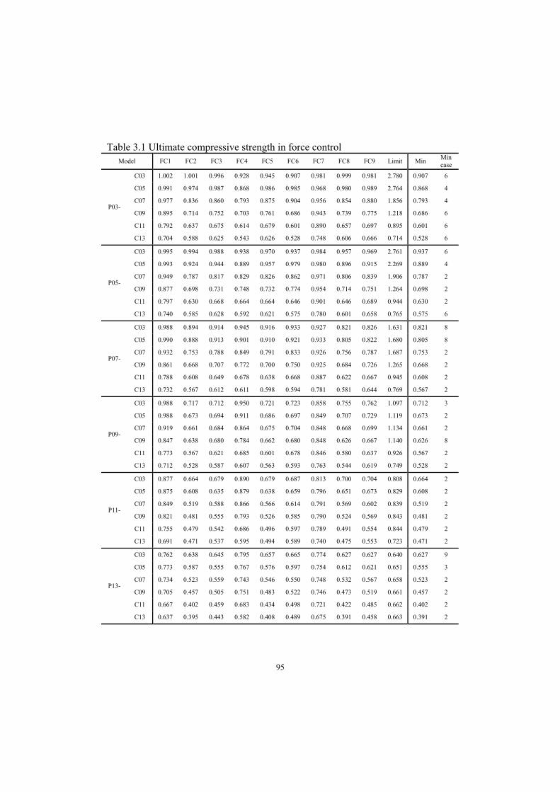
95

Table 3.1 Ultimate compressive strength in force controlModel FC1 FC2 FC3 FC4 FC5 FC6 FC7 FC8 FC9 Limit Min

Mincase

C03 1.002 1.001 0.996 0.928 0.945 0.907 0.981 0.999 0.981 2.780 0.907 6

C05 0.991 0.974 0.987 0.868 0.986 0.985 0.968 0.980 0.989 2.764 0.868 4

C07 0.977 0.836 0.860 0.793 0.875 0.904 0.956 0.854 0.880 1.856 0.793 4

C09 0.895 0.714 0.752 0.703 0.761 0.686 0.943 0.739 0.775 1.218 0.686 6

C11 0.792 0.637 0.675 0.614 0.679 0.601 0.890 0.657 0.697 0.895 0.601 6

P03-

C13 0.704 0.588 0.625 0.543 0.626 0.528 0.748 0.606 0.666 0.714 0.528 6

C03 0.995 0.994 0.988 0.938 0.970 0.937 0.984 0.957 0.969 2.761 0.937 6

C05 0.993 0.924 0.944 0.889 0.957 0.979 0.980 0.896 0.915 2.269 0.889 4

C07 0.949 0.787 0.817 0.829 0.826 0.862 0.971 0.806 0.839 1.906 0.787 2

C09 0.877 0.698 0.731 0.748 0.732 0.774 0.954 0.714 0.751 1.264 0.698 2

C11 0.797 0.630 0.668 0.664 0.664 0.646 0.901 0.646 0.689 0.944 0.630 2

P05-

C13 0.740 0.585 0.628 0.592 0.621 0.575 0.780 0.601 0.658 0.765 0.575 6

C03 0.988 0.894 0.914 0.945 0.916 0.933 0.927 0.821 0.826 1.631 0.821 8

C05 0.990 0.888 0.913 0.901 0.910 0.921 0.933 0.805 0.822 1.680 0.805 8

C07 0.932 0.753 0.788 0.849 0.791 0.833 0.926 0.756 0.787 1.687 0.753 2

C09 0.861 0.668 0.707 0.772 0.700 0.750 0.925 0.684 0.726 1.265 0.668 2

C11 0.788 0.608 0.649 0.678 0.638 0.668 0.887 0.622 0.667 0.945 0.608 2

P07-

C13 0.732 0.567 0.612 0.611 0.598 0.594 0.781 0.581 0.644 0.769 0.567 2

C03 0.988 0.717 0.712 0.950 0.721 0.723 0.858 0.755 0.762 1.097 0.712 3

C05 0.988 0.673 0.694 0.911 0.686 0.697 0.849 0.707 0.729 1.119 0.673 2

C07 0.919 0.661 0.684 0.864 0.675 0.704 0.848 0.668 0.699 1.134 0.661 2

C09 0.847 0.638 0.680 0.784 0.662 0.680 0.848 0.626 0.667 1.140 0.626 8

C11 0.773 0.567 0.621 0.685 0.601 0.678 0.846 0.580 0.637 0.926 0.567 2

P09-

C13 0.712 0.528 0.587 0.607 0.563 0.593 0.763 0.544 0.619 0.749 0.528 2

C03 0.877 0.664 0.679 0.890 0.679 0.687 0.813 0.700 0.704 0.808 0.664 2

C05 0.875 0.608 0.635 0.879 0.638 0.659 0.796 0.651 0.673 0.829 0.608 2

C07 0.849 0.519 0.588 0.866 0.566 0.614 0.791 0.569 0.602 0.839 0.519 2

C09 0.821 0.481 0.555 0.793 0.526 0.585 0.790 0.524 0.569 0.843 0.481 2

C11 0.755 0.479 0.542 0.686 0.496 0.597 0.789 0.491 0.554 0.844 0.479 2

P11-

C13 0.691 0.471 0.537 0.595 0.494 0.589 0.740 0.475 0.553 0.723 0.471 2

C03 0.762 0.638 0.645 0.795 0.657 0.665 0.774 0.627 0.627 0.640 0.627 9

C05 0.773 0.587 0.555 0.767 0.576 0.597 0.754 0.612 0.621 0.651 0.555 3

C07 0.734 0.523 0.559 0.743 0.546 0.550 0.748 0.532 0.567 0.658 0.523 2

C09 0.705 0.457 0.505 0.751 0.483 0.522 0.746 0.473 0.519 0.661 0.457 2

C11 0.667 0.402 0.459 0.683 0.434 0.498 0.721 0.422 0.485 0.662 0.402 2

P13-

C13 0.637 0.395 0.443 0.582 0.408 0.489 0.675 0.391 0.458 0.663 0.391 2

96

Table 3.2 Ultimate compressive strength in displacement controlModel DC1 DC2 DC3 DC4 DC5 DC6 DC7 DC8 DC9 Min

Mincase

C03 1.059 1.046 1.054 1.060 1.058 1.053 1.057 1.044 1.043 1.043 9

C05 1.030 0.970 0.996 1.031 0.998 0.973 1.033 0.981 0.972 0.970 2

C07 1.001 0.867 0.896 1.009 0.907 0.883 1.012 0.896 0.885 0.867 2

C09 0.972 0.784 0.831 0.986 0.853 0.823 0.995 0.806 0.833 0.784 2

C11 0.927 0.742 0.793 0.945 0.808 0.776 0.983 0.775 0.792 0.742 2

P03-

C13 0.879 0.708 0.773 0.900 0.785 0.735 0.974 0.745 0.761 0.708 2

C03 1.043 1.021 1.030 1.047 1.039 1.028 1.025 0.983 0.976 0.976 9

C05 1.014 0.926 0.955 1.018 0.959 0.933 1.012 0.922 0.895 0.895 9

C07 0.988 0.827 0.882 0.998 0.890 0.856 1.002 0.861 0.860 0.827 2

C09 0.963 0.775 0.826 0.979 0.830 0.806 0.989 0.800 0.812 0.775 2

C11 0.936 0.738 0.798 0.947 0.794 0.763 0.980 0.765 0.774 0.738 2

P05-

C13 0.902 0.711 0.773 0.917 0.775 0.727 0.972 0.743 0.746 0.711 2

C03 1.036 0.939 0.952 1.038 0.944 0.943 0.974 0.887 0.890 0.887 8

C05 1.006 0.891 0.930 1.013 0.924 0.915 0.983 0.858 0.850 0.850 9

C07 0.982 0.816 0.877 0.993 0.877 0.848 0.979 0.813 0.821 0.813 8

C09 0.960 0.767 0.827 0.977 0.819 0.796 0.977 0.785 0.785 0.767 2

C11 0.937 0.734 0.799 0.952 0.784 0.754 0.976 0.758 0.755 0.734 2

P07-

C13 0.911 0.710 0.769 0.927 0.775 0.720 0.973 0.742 0.728 0.710 2

C03 1.021 0.805 0.810 1.022 0.797 0.792 0.935 0.828 0.795 0.792 6

C05 0.992 0.791 0.804 0.991 0.805 0.780 0.929 0.790 0.774 0.774 9

C07 0.958 0.774 0.786 0.934 0.797 0.773 0.903 0.772 0.771 0.771 9

C09 0.952 0.756 0.788 0.931 0.793 0.764 0.898 0.762 0.745 0.745 9

C11 0.928 0.730 0.781 0.946 0.776 0.745 0.890 0.751 0.724 0.724 9

P09-

C13 0.912 0.707 0.759 0.902 0.769 0.713 0.887 0.740 0.697 0.697 9

C03 0.895 0.756 0.772 0.891 0.749 0.758 0.888 0.792 0.759 0.749 5

C05 0.873 0.732 0.741 0.867 0.749 0.725 0.861 0.747 0.732 0.725 6

C07 0.867 0.710 0.725 0.851 0.728 0.715 0.841 0.718 0.722 0.710 2

C09 0.853 0.696 0.715 0.846 0.715 0.694 0.830 0.701 0.703 0.694 6

C11 0.852 0.693 0.699 0.832 0.708 0.666 0.825 0.695 0.685 0.666 6

P11-

C13 0.862 0.660 0.678 0.827 0.700 0.673 0.820 0.697 0.658 0.658 9

C03 0.846 0.751 0.756 0.816 0.755 0.726 0.873 0.776 0.743 0.726 6

C05 0.833 0.712 0.712 0.829 0.728 0.705 0.838 0.727 0.716 0.705 6

C07 0.822 0.680 0.697 0.808 0.704 0.687 0.814 0.691 0.678 0.678 9

C09 0.817 0.660 0.688 0.790 0.693 0.631 0.802 0.673 0.678 0.631 6

C11 0.816 0.640 0.628 0.780 0.681 0.637 0.794 0.660 0.642 0.628 3

P13-

C13 0.806 0.636 0.607 0.775 0.679 0.581 0.785 0.655 0.627 0.581 6

97

Fig 3.9 Inelastic buckling modes of flanges stiffened with U-rib at ultimate andfracture states

PLB at ultimate

CBP at ultimate

CBN at ultimate

Interaction of PLB & CBPat ultimate

Interaction of PLB & CBPat fracture

Interaction of PLB & CBNat fracture

Interaction of PLB & CBNat ultimate

PLB at fracture

CBP at fracture

CBN at fracture

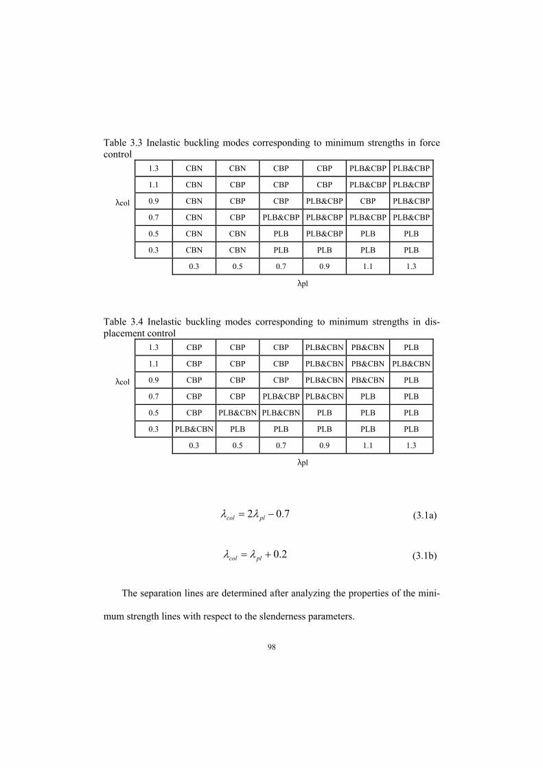
98

Table 3.3 Inelastic buckling modes corresponding to minimum strengths in forcecontrol

1.3 CBN CBN CBP CBP PLB&CBP PLB&CBP

1.1 CBN CBP CBP CBP PLB&CBP PLB&CBP

0.9 CBN CBP CBP PLB&CBP CBP PLB&CBP

0.7 CBN CBP PLB&CBP PLB&CBP PLB&CBP PLB&CBP

0.5 CBN CBN PLB PLB&CBP PLB PLB

λcol

0.3 CBN CBN PLB PLB PLB PLB

0.3 0.5 0.7 0.9 1.1 1.3

λpl

Table 3.4 Inelastic buckling modes corresponding to minimum strengths in dis-placement control

1.3 CBP CBP CBP PLB&CBN PB&CBN PLB

1.1 CBP CBP CBP PLB&CBN PB&CBN PLB&CBN

0.9 CBP CBP CBP PLB&CBN PB&CBN PLB

0.7 CBP CBP PLB&CBP PLB&CBN PLB PLB

0.5 CBP PLB&CBN PLB&CBN PLB PLB PLB

λcol

0.3 PLB&CBN PLB PLB PLB PLB PLB

0.3 0.5 0.7 0.9 1.1 1.3

λpl

7.02 plcol (3.1a)

2.0 plcol (3.1b)

The separation lines are determined after analyzing the properties of the mini-

mum strength lines with respect to the slenderness parameters.

99

Fig 3.10 Simplified inelastic buckling modes: (a) Force control (b) Displace-ment control

0.3 0.5 0.7 0.9 1.1 1.3pl

col

0.3

0.5

0.7

0.9

1.1

1.3

Column-type bucklingInteractionPlate-type buckling

2.0 plcol

(b)

(a)0.3 0.5 0.7 0.9 1.1 1.3 pl

col

0.3

0.5

0.7

0.9

1.1

1.3

Column-type bucklingInteractionPlate-type buckling

7.02 plcol

100

To investigate influences of the plate slenderness parameter pl on the mini-

mum strength lines, series C03 to C13 are analyzed. The pl for each series vary

from 0.3 to 1.3. Similarly, series P03 to P13 are analyzed to investigate influ-

ences of the column slenderness parameter col on the minimum strength lines.

Fig. 3.11 and 3.12 show the minimum strength lines with respect pl . For each

column slenderness parameter, the strength generally decreases when pl is at

least some level greater than col . Roughly, pl maintains a certain level at the

column-like behavior but decreases rapidly at the plate-like behavior. Consider-

ing this property, a division line between the plate-like behavior and the column-

like behavior can be determined. The line in the force and displacement controls

is indicated in Eq. (3.1a) and (3.1b), respectively. Generally, the ultimate com-

pressive strength is not governed alone by the plate slenderness parameter without

the plate-like behavior. This explains that the relative relationship between pl

and col is more important in the behaviors of stiffened flanges. Fig. 3.13 and

3.14 show the col effect on the minimum strength lines. Unlike Fig. 3.11 and

3.12, the strength nearly decreases as col increases. The pattern roughly seems

to be linear. The strength also decreases as pl increases.

101

0

0.2

0.4

0.6

0.8

1

1.2

0.2 0.4 0.6 0.8 1 1.2 1.4

Lambda C = 0.3Lambda C = 0.5Lambda C = 0.7Lambda C = 0.9Lambda C = 1.1Lambda C = 1.3

Fu /

Fy

pl

Plate likebehavior

Column likebehavior

Separation line

Fig. 3.11 Minimum strength lines with respect to plate slenderness parameterin force control

0

0.2

0.4

0.6

0.8

1

1.2

0.2 0.4 0.6 0.8 1 1.2 1.4

Lambda C = 0.3Lambda C = 0.5Lambda C = 0.7Lambda C = 0.9Lambda C = 1.1Lambda C = 1.3

Fu /

Fy

All plate behavior

pl

Plate likebehavior

Column likebehavior

Separation line

Fig. 3.12 Minimum strength lines with respect to plate slenderness parameterin displacement control

102

0

0.2

0.4

0.6

0.8

1

1.2

0.2 0.4 0.6 0.8 1 1.2 1.4

Lambda P = 0.3Lambda P = 0.5

Lambda P = 0.7Lambda P = 0.9

Lambda P = 1.1Lambda P = 1.3

Fu /

Fy

Linearly decreasing

col

Fig. 3.13 Minimum strength lines with respect to column slendernessparameter in force control

0

0.2

0.4

0.6

0.8

1

1.2

0.2 0.4 0.6 0.8 1 1.2 1.4

Lambda P = 0.3

Lambda P = 0.5

Lambda P = 0.7Lambda P = 0.9

Lambda P = 1.1Lambda P = 1.3

Fu /

Fy

col

Linearly decreasing

Fig. 3.14 Minimum strength lines with respect to column slenderness parame-ter in displacement control

103

3.4 Influence of initial geometric imperfection

The series P07 in Table 2.4 are analyzed to evaluate influences of the initial

geometric imperfections (defined in section 2.4). The models have intermediate

thickness with td=12.671mm, and longitudinal length L from 2.018m to 8.746m.

Figs. 3.15(a) and 3.15(b) show an influence of the initial geometric imperfec-

tion shapes on the ultimate compressive strength of the stiffened flanges with U-

ribs under the condition of not-considered residual stresses. More variation oc-

curs in the force control rather than the displacement control due to a relatively

weak constraint effect. If we compare Case 1 to Case 4 in 3.15(a), CBP triggers a

higher strength than CBN. Since the initial imperfection shape is similar to the

final inelastic buckling mode. It is generally known that the positive column-type

buckling strength is higher than the negative column-type buckling strength

(Sheikh et al., 2002). Unlike the minimum strength lines in Fig. 3.13 and 3.14,

the strength decreases after maintaining a certain constant level. Horizontal and

decreasing lines indicate the plate-like behavior and the column-like behavior, re-

spectively. From the results, we reveal that initial imperfection of the PLB shape

produces the stronger plate-like behavior. The initial imperfection of other shapes

can be explained in the same way. However, initial imperfection shape and ine-

lastic buckling modes may not be consistent.

104

0

0.2

0.4

0.6

0.8

1

1.2

0.2 0.4 0.6 0.8 1 1.2 1.4

1. FC-CBP-RSX

4. FC-CBN-RSX

7. FC-PLB-RSX

Fu /

Fy

col

(a)

Plate-like behavior

Column-like behavior

0

0.2

0.4

0.6

0.8

1

1.2

0.2 0.4 0.6 0.8 1 1.2 1.4

1. DC-CBP-RSX

4. DC-CBN-RSX

7. DC-PLB-RSX

Fu /

Fycol

(b)

All plate behavior

Plate-like behavior

Column-like behavior

0

0.2

0.4

0.6

0.8

1

1.2

0.2 0.4 0.6 0.8 1 1.2 1.4

2. FC-CBP-RSO

5. FC-CBN-RSO

8. FC-PBL-RSO

Fu /

Fy

col

(c)

Plate-like behavior

Column-like behavior

0

0.2

0.4

0.6

0.8

1

1.2

0.2 0.4 0.6 0.8 1 1.2 1.4

2. DC-CBP-RSO

5. DC-CBN-RSO

8. DC-PLB-RSO

Fu /

Fy

col

(d)

Plate-like behavior

Column-like behavior

0

0.2

0.4

0.6

0.8

1

1.2

0.2 0.4 0.6 0.8 1 1.2 1.4

3. FC-CBP-RSR

6. FC-CBN-RSR

9. FC-PLB-RSR

Fu /

Fy

col

(e)

Plate-like behavior

Column-like behavior

0

0.2

0.4

0.6

0.8

1

1.2

0.2 0.4 0.6 0.8 1 1.2 1.4

3. DC-CBP-RSR

6. DC-CBN-RSR

9. DC-PLB-RSR

Fu /

Fy

col

(f)

Plate-like behavior

Column-like behavior

Fig 3.15 Influence of initial geometric imperfection shapes on ultimate com-pressive strength of series P07: (a) FC and (b) DC with no residual stress, (c) FC

and (d) DC with simply-considered residual stress, (e) FC and (f) DC with recoveryof residual stress effect.

105

Figs. 3.15(c) and 3.15(d) show an influence of the initial imperfection shapes

on the ultimate compressive strength of the stiffened flanges under the condition of

simply-considered residual stress. For low col , all cases show the plate-like

behavior regardless of the initial imperfection shapes due to the local effect of

compressive residual stress distributed over most of the flange (local effect of

residual stress). The strength of PLB is lesser than the strength of CBP or CBN.

The maximum difference (reduction) of the strength is approximately 10%. The-

se results explain that the initial imperfection shape, which is closer to the final

inelastic buckling mode, plays a significant role. col is larger than a certain

value, which shows the column-like behavior, and mostly the influence of the ini-

tial imperfection shape on the ultimate strength, which is not large. Comparing

Case 7 in 3.15(a) and Case 8 in 3.15(c), the effect of an unbalanced moment from

the longitudinal residual stress (global effect of residual stress) produces the stron-

ger column-like behavior. Fig. 3.16 shows a vertical displacement pattern by the re-

Fig. 3.16 Vertical displacement (m) by residual stresses redistribution in per-fect stiffened flange (P07-C07 model)

106

distribution effect of residual stresses in a perfect stiffened flange. The pattern is

very similar to initial geometric imperfection of the CBP shape. The fractures of

all cases occur in the shape of positive column-type buckling because the influence

of the redistribution of residual stress is larger than an influence of the initial

geometric imperfection. For this reason, initial imperfection of the CBP shape

leads to lower strength than that of the CBN shape. If the magnitude of initial

imperfection of the CBN shape is much greater than the displacements by the re-

distribution effect of residual stresses, then the failure mode will be negative col-

umn-type buckling.

An influence of the initial imperfection shapes with recovery of the redistribu-

tion effect of residual stresses are also analyzed in Figs. 3.15(e) and 3.15(f). The

influence is not large except at a low col such as in Figs. 3.15(c) and 3.15(d).

However, there are some differences in the strength curve and failure patterns. In

Figs. 3.15(e) and 3.15(f), Case 6 has a lower strength than Case 3 at a large col in

the force control and at all ranges of col in the displacement control because the

fracture modes of Case 6 and Case 3 are negative column-type buckling and posi-

tive column-type buckling, respectively. These results denote that an influence of

total initial imperfection (original initial imperfection and additional initial imper-

fection from recovery of the redistribution effect of residual stresses) is greater than

the global effect of residual stress.

During the analyses, Case 6 in 3.15(e) showed unexpected behaviors from 0.7

107

to 0.9 at the col . When compressive forces are applied to a stiffened flange after

the recovery process, most of the vertical displacements start to move in the nega-

tive (column-type buckling) direction. However, the vertical displacements

change direction at certain points and finally the stiffened flange is fractured in a

positive (column-type buckling) direction. In view of only the traced points, it

appears similar to a snap-through. Case 5 in 3.15(d) showed similar results from

0.7 to 1.3 at the col . More details are described in section 3.6.

In summary, if residual stresses are not considered, the influence of the initial

imperfection shapes on the ultimate strength is large in the force control, but not in

the displacement control. If residual stresses are considered, the influence of ini-

tial imperfection of the PLB shape is significant if the fracture mode is the plate-

type buckling due to the local effect of residual stresses. The maximum reduction

is approximately 10% compared to the other cases. However, the influence of the

initial imperfection shapes is not significant if the fracture mode is the column-type

buckling due to the dominant global effect of residual stresses.

108

3.5 Influence of residual stresses

According to the results by Chou et al. (2006), the influence of residual stress is

more significant than the influence of initial geometric imperfection in the buckling

behavior. In order to quantitatively evaluate the effects of residual stresses on the

ultimate compressive strength of wide stiffened flanges with U-ribs, series C03

through series C13 are analyzed with respect to pl . Series C03 (short plate) and

series C13 (long plate) have longitudinal length of 1.629m to 2.183m and 7.061m

to 9.46m, respectively. The thickness of the stiffened flanges varies from

6.823mm to 29.565mm. Details of the geometry for the other series are written in

Table 2.4. For initial geometric imperfection, CBP (positive column-type buck-

ling mode) is involved. Based on critical stress when the stiffened flange is free

of residual stress (Case 1), a reduction effect by the presence of residual stress on

the ultimate strength are evaluated with absolute and relative values, which are

summarized in Table 3.5. Roughly, the residual stresses decrease the strength by

0~40% in the force control and 0~25% in the displacement control. According to

Grondin et al. (1999), residual stresses in the plate decrease the strength roughly in

direct proportion to the magnitude of the compressive residual stresses in the plate-

like behavior. Relatively lower strength reduction occurs in the column-like be-

havior compared to the plate-like behavior. Considering that the magnitude of

compressive residual stress in this study is yF25.0 (25%), the reduction effect

109

seems to be significant in the force control.

Fig. 3.17 shows the ultimate compressive strength versus pl for series C03

(short plate), series C09 (near intermediate plate) and series C13 (long plate),

where Case 1 is not-considered residual stresses, Case 2 is simply-considered

residual stresses and Case 3 is recovery of residual stress effect. In the ultimate

strength versus pl , the horizontal strength line denotes the column-like behavior

and the decreasing strength line denotes the plate-like behavior. Generally, abso-

lute maximum reduction occurs at the point where the mode of failure changes

from the column-type buckling to the plate-type buckling in terms of Case 1.

Strength reduction by residual stress is larger in the force control than in the dis-

placement control. This can also be described as an additional constraint effect in

the displacement control.

Figs. 3.17(a) and 3.17(b) show that recovery of the redistribution effect of

residual stresses is negligible for the short flanges ( 3.0col ). Since pl is

greater than col , behaviors of the stiffened flange is governed dominantly by the

compressive residual stress over all plates rather than by the presence of an addi-

tional column type initial imperfection from the redistribution effect of residual

stress. In other words, residual stress produces stronger plate-like behavior.

Therefore, Case 2 or Case 3 shows earlier plate-like behavior than Case 1 as pl

increases.

Figs. 3.17(c) and 3.17(d) show the results of the stiffened flanges, which have

110

9.0col . In this case, recovery of the redistribution effect of residual stress

noticeably contributes to the ultimate strength. Case 3 is higher than Case 2 with

yF04.0 ~yF07.0 and

yF02.0 ~yF06.0 in absolute magnitude by the force and dis-

placement control, respectively.

Figs. 3.17(e) and 3.17(f) show the results for the long stiffened flange

( 3.1col ). The variation of the strength reduction by residual stress is not large

in comparison to the short flange. When strength decreases after maintaining a

certain level, the stiffened flange is governed by the plate-like behavior with the

minor column-like behavior. Specifically, this range belongs to the interaction.

In 3.17(f), strength by RSR is lower than RSO at 3.1pl because RSO produce

an interaction of PLB-CBP. However, RSR produces an interaction of PLB-CBN.

Thus, strength by CBN is lower than CBP.

111

0

0.2

0.4

0.6

0.8

1

1.2

0.2 0.4 0.6 0.8 1 1.2 1.4

1. FC-CBP-RSX

2. FC-CBP-RSO

3. FC-CBP-RSR

Fu /

Fy

pl

(a)

- 28%

Absolute max reduction = 0.276Fy

Relative max reduction

0

0.2

0.4

0.6

0.8

1

1.2

0.2 0.4 0.6 0.8 1 1.2 1.4

1. DC-CBP-RSX

2. DC-CBP-RSO

3. DC-CBP-RSR

Fu /

Fypl

(b)

- 21.2%

Absolute max reduction = 0.216Fy

Relative max reduction

0

0.2

0.4

0.6

0.8

1

1.2

0.2 0.4 0.6 0.8 1 1.2 1.4

1. FC-CBP-RSX

2. FC-CBP-RSO

3. FC-CBP-RSR

Fu /

Fy

pl

(c)

- 41.4%

Absolute max reduction = 0.340Fy

Relative max reduction

0

0.2

0.4

0.6

0.8

1

1.2

0.2 0.4 0.6 0.8 1 1.2 1.4

1. DC-CBP-RSX

2. DC-CBP-RSO

3. DC-CBP-RSR

Fu /

Fy

pl

(d)

- 20.5%

Absolute max reduction = 0.195Fy

Relative max reduction

0

0.2

0.4

0.6

0.8

1

1.2

0.2 0.4 0.6 0.8 1 1.2 1.4

1. FC-CBP-RSX

2. FC-CBP-RSO

3. FC-CBP-RSR

Fu /

Fy

pl

(e)

- 38%

Absolute max reduction = 0.242Fy

Relative max reduction

0

0.2

0.4

0.6

0.8

1

1.2

0.2 0.4 0.6 0.8 1 1.2 1.4

1. DC-CBP-RSX

2. DC-CBP-RSO

3. DC-CBP-RSR

Fu /

Fy

pl

(f)

- 24.7%

Absolute max reduction = 0.205Fy

Relative max reduction

Fig 3.17 Influence of residual stress on ultimate compressive strength:strengths of series C03 (short plate) in (a) FC and (b) DC, strength of series C09 in

(c) FC and (d) DC, strengths of series C13 (long plate) in (e) FC and (f) DC. Allmodels consider CBP shape of initial geometric imperfection.

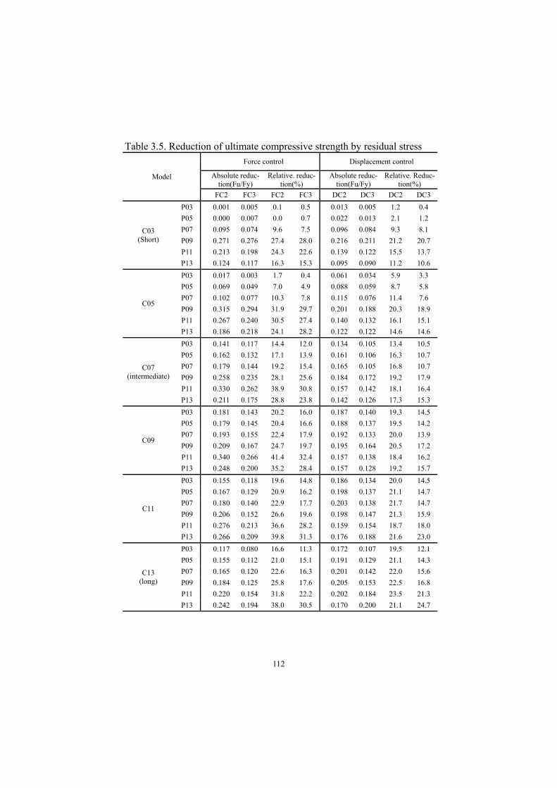
112

Table 3.5. Reduction of ultimate compressive strength by residual stress

Force control Displacement control

Absolute reduc-tion(Fu/Fy)

Relative. reduc-tion(%)

Absolute reduc-tion(Fu/Fy)

Relative. Reduc-tion(%)

Model

FC2 FC3 FC2 FC3 DC2 DC3 DC2 DC3

P03 0.001 0.005 0.1 0.5 0.013 0.005 1.2 0.4

P05 0.000 0.007 0.0 0.7 0.022 0.013 2.1 1.2

P07 0.095 0.074 9.6 7.5 0.096 0.084 9.3 8.1

P09 0.271 0.276 27.4 28.0 0.216 0.211 21.2 20.7

P11 0.213 0.198 24.3 22.6 0.139 0.122 15.5 13.7

C03(Short)

P13 0.124 0.117 16.3 15.3 0.095 0.090 11.2 10.6

P03 0.017 0.003 1.7 0.4 0.061 0.034 5.9 3.3

P05 0.069 0.049 7.0 4.9 0.088 0.059 8.7 5.8

P07 0.102 0.077 10.3 7.8 0.115 0.076 11.4 7.6

P09 0.315 0.294 31.9 29.7 0.201 0.188 20.3 18.9

P11 0.267 0.240 30.5 27.4 0.140 0.132 16.1 15.1

C05

P13 0.186 0.218 24.1 28.2 0.122 0.122 14.6 14.6

P03 0.141 0.117 14.4 12.0 0.134 0.105 13.4 10.5

P05 0.162 0.132 17.1 13.9 0.161 0.106 16.3 10.7

P07 0.179 0.144 19.2 15.4 0.165 0.105 16.8 10.7

P09 0.258 0.235 28.1 25.6 0.184 0.172 19.2 17.9

P11 0.330 0.262 38.9 30.8 0.157 0.142 18.1 16.4

C07(intermediate)

P13 0.211 0.175 28.8 23.8 0.142 0.126 17.3 15.3

P03 0.181 0.143 20.2 16.0 0.187 0.140 19.3 14.5

P05 0.179 0.145 20.4 16.6 0.188 0.137 19.5 14.2

P07 0.193 0.155 22.4 17.9 0.192 0.133 20.0 13.9

P09 0.209 0.167 24.7 19.7 0.195 0.164 20.5 17.2

P11 0.340 0.266 41.4 32.4 0.157 0.138 18.4 16.2

C09

P13 0.248 0.200 35.2 28.4 0.157 0.128 19.2 15.7

P03 0.155 0.118 19.6 14.8 0.186 0.134 20.0 14.5

P05 0.167 0.129 20.9 16.2 0.198 0.137 21.1 14.7

P07 0.180 0.140 22.9 17.7 0.203 0.138 21.7 14.7

P09 0.206 0.152 26.6 19.6 0.198 0.147 21.3 15.9

P11 0.276 0.213 36.6 28.2 0.159 0.154 18.7 18.0

C11

P13 0.266 0.209 39.8 31.3 0.176 0.188 21.6 23.0

P03 0.117 0.080 16.6 11.3 0.172 0.107 19.5 12.1

P05 0.155 0.112 21.0 15.1 0.191 0.129 21.1 14.3

P07 0.165 0.120 22.6 16.3 0.201 0.142 22.0 15.6

P09 0.184 0.125 25.8 17.6 0.205 0.153 22.5 16.8

P11 0.220 0.154 31.8 22.2 0.202 0.184 23.5 21.3

C13(long)

P13 0.242 0.194 38.0 30.5 0.170 0.200 21.1 24.7

113

3.6 Snap-though like phenomenon in stiffened flanges with U-

ribs

An unexpected behavior such that a mode of deflection changes before reaching

the maximum load occurs in the stiffened flanges with U-ribs. In this section, we

discuss the cause and impact of the unexpected behavior on the ultimate compres-

sive strength of stiffened flanges. Next, we discuss snap-through like phenome-

non.

Fig 3.18 shows the load-displacement curve of the P07-C09 model by FC6

(FC-CBN-RSR). The models have td=12.671mm and L=6.055m. In the sign

convention, a negative half sign curve has a positive value in a given coordinate.

Due to the recovering process for the distortion from the redistribution effect of

residual stress, we have the desired shape and magnitude of initial imperfection

(L/1000=6.055mm) before the compression run. As compressive force increase,

the magnitude of longitudinal shortening increases along the A→B→C path. The

notable thing is that the stiffness of the stiffened flange starts to decease rapidly

from point B. Fig. 3.19 shows vertical displacement versus compressive force at

the center node of this model. As the compressive force increases, vertical dis-

placement also increases from A to B, but abruptly changes direction at B and fi-

nally reaches an ultimate state at C with a positive column-type buckling shape.

In other words, the mode of deflection is changed before reaching the maximum

114

load.

More wide observations are performed on the longitudinal and transverse

centerline of the stiffened flange as shown in Figs. 3.20(a) and 3.20(b). A history

of vertical locations is traced based on the undeformed perfect system in order to

know the configuration of the stiffened flange containing initial imperfection.

The undeformed perfect system has vertical locations equal to zero due to no initial

geometric imperfection. As shown in Figs. 3.20(a) and 3.20(b), longitudinal or

transverse displacements in the stiffened flange starts to change direction at point B

and the system finally reaches an ultimate state at point C after the system changes

the global configuration mode gradually from point B to point C. Thus, we can

presume that the points changing direction of vertical displacement coincide with

the points losing a large amount of stiffness.

Active yield stresses are investigated from state A to state C to confirm this

supposition (Fig. 3.21), where red elements denote yield states and blue elements

do not-yield state. Precisely, stiffened flange starts to express stiffness loss in the

center areas at turning point B. Consequently, it is believed that the yielding area

of the stiffened flange contribute to stiffness loss and lead to changing the direction

of displacement.

The traced points from B to C in Fig. 3.20 resemble a snap-through pattern.

However, the traced points are not a snap-through pattern. The deflection mode is

changed gradually before reaching the maximum load due to the remained stiffness.

This is unlike real snap-through phenomenon, which shows a sudden jump from

115

one equilibrium configuration to another equilibrium configuration after reaching

the maximum load. Hence, this phenomenon for convenience will be called snap-

through like phenomenon in this study.

A snap-through like phenomenon also occurred from DC5 (DC-CBN-RSO).

Fig. 3.22 shows compressive force versus longitudinal shortening response for the

above P07-C09 model. Fig. 3.23 shows a vertical displacement response versus a

compressive force for the same model. Like the FC6 case, the stiffness of the

system starts to decrease from point B at the moment of changing the direction of

the vertical displacement. The stiffness loss is also confirmed with the yielding

area of the stiffened flange as shown in Fig. 3.25. However, Fig. 3.24 shows that

the history of vertical locations along the longitudinal or transverse centerline does

not go above zero. The magnitude of vertical displacement was small in compari-

son to the force control because the property of the displacement control contribut-

es to an additional constraint effect. The variation from point B to point C is not

large in comparison to the force control. Thus, the global configuration mode

does not change despite that the mode of deflection changes.

Among the eighteen inelastic buckling analysis cases introduced in Table 2.6,

some geometric models in FC6 and DC5 show snap-through like phenomenon.

Most of the geometric models in FC6 also show a change in the global configura-

tion mode unlike DC5. The strengths at the starting point of snap-through like

phenomenon are summarized in Table 3.6.

116

0

0.2

0.4

0.6

0.8

1

0 5 10 15 20

LD curveA. Starting pointB. Turning pointC. Ultimate point

Longitudinal shortening (mm)

Com

pres

sive

for

ce (

F /

Fy)

A

BC

Ux

P = F/Fyx

y

z

(8.9mm, 0.75Fy)

Fig. 3.18 Compression versus longitudinal shortening for P07-C09 model inFC6

-80

-60

-40

-20

0

20

40

0 0.2 0.4 0.6 0.8 1

Vertical displacementA. Stating pointB. Turning pointC. Ultimate point

Compressive force (F/Fy)

A (0, 0mm)

B (0.92Fu, 6.17mm)

C (Fu, -59.5mm)P = F/Fy

Uyx

y

z

Ver

tical

dis

plac

emen

t (m

m)

Fig. 3.19 Vertical displacement versus Compression for P07-C09 model inFC6

117

-60

-40

-20

0

20

40

60

0 1 2 3 4 5 6

A. Starting points (P = 0)B. Turning points (P = 0.92Fu)m. (P=0.97Fu)C. Ultimate points (P = Fu)

Longitudinal Distance (m)

Ver

tical

loca

tion

(m

m)

A

B

C

(a)

m

-60

-40

-20

0

20

40

60

0 1 2 3 4 5 6 7 8

A. Starting points (P = 0)B. Turning points (P = 0.92Fu)m. (P=0.97Fu)C. Ultimate points (P = Fu)

Transverse Distance (m)

Ver

tical

loca

tion

(m

m)

A

B

C

(b)

m

Fig. 3.20 History of vertical locations at (a) longitudinal centerline and (b)transverse centerline of P07-C09 model in FC6

118

Fig. 3.21 Yielding area of P07-C09 model in FC6: (a) Starting points A, (b)Turning points B, (c) Ultimate points C.

119

0

0.2

0.4

0.6

0.8

1

0 2 4 6 8 10

LD curveA. Starting pointB. Turning pointC. Ultimate point

Longitudinal shortening (mm)

Com

pres

sive

for

ce (

F /

Fy)

A

B

C

Ux

Ux

x

y

z

Fig. 3.22 Compression versus longitudinal shortening for P07-C09 model inDC5

-30

-20

-10

0

10

20

0 0.2 0.4 0.6 0.8 1

Vertical displacementA. Stating pointB. Turning pointC. Ultimate point

Compressive force (F/Fy)

Ver

tical

dis

plac

emen

t (m

m)

A (0, 0mm)

Ux

Uy

B (0.83Fu, 3.36mm)

C (Fu, -17.7mm)

x

y

z

Fig. 3.23 Vertical displacement versus Compression for P07-C09 model inDC5

120

-30

-20

-10

0

10

20

30

0 1 2 3 4 5 6

A. Starting points (P = 0)

B. Turning points (P = 0.83Fu)

C. Ultimate points (P = Fu)

Longitudinal Distance (m)

Ver

tical

loca

tion

(m

m)

A

B

C

(a)

max = -1.7mm

max = -5.1mm

max = -23.7mm

-30

-20

-10

0

10

20

30

0 1 2 3 4 5 6 7 8

A. Starting points (P = 0)

B. Turning points (P = 0.83Fu)

C. Ultimate points (P = Fu)

Transverse Distance (m)

Ver

tical

loca

tion

(m

m)

A

B

C

(b)

Fig. 3.24 History of vertical locations at (a) longitudinal centerline and (b)transverse centerline of P07-C09 model in DC5

121

Fig. 3.25 Yielding area of P07-C09 model in DC5: (a) Starting points A, (b)Turning points B, (c) Ultimate points C.

122

Table 3.6 Strength at starting points of snap-through like phenomenon in (a) FC6and (b) DC5

(a) FC6 (FC-CBN-RSR) (b) DC5 (DC-CBN-RSO)Model

Fu DET Fss Fss/Fu

Model

Fu DET Fss Fss/Fu

C03 0.907 X 0.829 0.914 C09 0.853 X 0.701 0.822

C05 0.985 O 0.760 0.772 C11 0.808 X 0.642 0.794P03-

C07 0.904 O 0.723 0.799

P03-

C13 0.785 X 0.712 0.908

C03 0.937 X 0.794 0.848 C07 0.890 X 0.723 0.812

C05 0.979 O 0.713 0.728 C09 0.830 X 0.678 0.817

C07 0.862 O 0.680 0.789 C11 0.794 X 0.706 0.890P05-

C09 0.774 O 0.713 0.920

P05-

C13 0.775 X 0.705 0.910

C05 0.921 O 0.695 0.755 C07 0.877 X 0.766 0.873

C07 0.833 O 0.680 0.816 C09 0.819 X 0.682 0.833P07-

C09 0.750 O 0.693 0.924 C11 0.784 X 0.748 0.954

C05 0.697 O 0.687 0.986

P07-

C13 0.775 X 0.709 0.914

C07 0.704 O 0.660 0.937 C09 0.793 X 0.672 0.847P09-

C09 0.680 O 0.663 0.974 C11 0.776 X 0.728 0.937

C07 0.614 O 0.579 0.942

P09-

C13 0.769 X 0.706 0.918

C09 0.585 O 0.577 0.986P11-

C11 0.597 O 0.597 1.000

C07 0.550 O 0.400 0.727

C09 0.522 O 0.371 0.788

C11 0.498 O 0.405 0.814P13-

C13 0.489 O 0.439 0.897

DET: O = Change of global configuration mode, X = No change of global configuration mode

When the snap-through like phenomenon occurs, the phenomenon began at

70~100% and 80%~100% of the ultimate strength in FC6 and DC5, respectively.

Based on the data, occurrence patterns are analyzed with respect to the slenderness

parameters as shown in Fig. 3.26. The results shows that the snap-through like

phenomenon in FC6 has a bandwidth and that in DC5 has a local region. Related

to these patterns, more studies are required.

The process in FC6 provides a means for the stiffened flanges to have a de-

123

sired initial geometric imperfection (CBN) due to recovery of the redistribution

effect of residual stress. In other words, the configurations of the stiffened flanges

before applying compressive force are above the horizontal line (zero value) under

the given coordinate. As the compressive force increases, vertical displacement

of the stiffened flanges increases in a positive direction (i.e., positive direction in

the given coordinate corresponds with the negative column-buckling mode). If a

snap-through like phenomenon does not occur, the system will represent negative

column-like behavior. However, the phenomenon occurs due to the stiffness loss

in the stiffened flanges and triggered the change of a global configuration mode

except for the P03-C03 and P05-C03 models as shown in Table 3.6. The excep-

tions reach the ultimate state before falling below the horizontal line due to the

properties of very short plates. The P03-C03 and P05-C03 models shows nega-

tive column-like behavior and become the lowest strength for the nine cases

(FC1~FC9). Thus, we can expect that snap-through like phenomenon leads to an

increase of the ultimate strength, except for very short plates because the strength

by positive column-like behavior is greater than the strength by negative column-

like behavior in an ultimate state.

The process by DC5 (DC-CBN-RSO) produces an additional initial imperfec-

tion of CBP shape due to the redistribution effect of residual stress. The direction

of the additional initial imperfection is opposite to the original initial imperfection

(CBN). The magnitude of additional initial imperfections of the P03~P13 series

are plotted along the longitudinal length in Fig. 3.27. If we compare the addition-

124

al initial imperfections with the original initial imperfections for the models in of

Table 3.6(b), the additional initial imperfections are 1.25 to 2.6 times larger than

the original initial imperfections. Thus, the configurations of the stiffened flanges

are under the horizontal line (zero value) before applying compressive force.

Even if the configuration of the stiffened flanges is CBP shape before compression,

the vertical displacements start to increase in an opposite direction of the shape as

shown in Fig. 3.19, because the direction of displacements is determined by overall

stress distribution from the sum of the residual stresses and the compressive force

of the stiffened flanges. However, the direction is changed after a snap-through

like phenomenon. Similar to the FC6, snap-through like phenomenon leads to an

increase of strength in the DC5.

Even if snap-through like phenomenon occurs, to consider the strength at the

starting point of this phenomenon as the ultimate compressive strength is too early

because the stiffened flanges with U-ribs still have stiffness characteristics.

125

Fig. 3.26 Occurrence pattern of snap-through like phenomenon in (a) FC6 withchange of global configuration mode and (b) DC5 without change of global con-

figuration mode.

(b) 0.3 0.5 0.7 0.9 1.1 1.3 pl

col

0.3

0.5

0.7

0.9

1.1

1.3

Snap-through like phenomenon only

7.0col

9.0pl

0.3 0.5 0.7 0.9 1.1 1.3 pl

col

0.3

0.5

0.7

0.9

1.1

1.3

Snap-through like phenomenon with changeof global configuration mode

3

2.2

3

1 plcol

3

1.0

3

1 plcol

(a)

Snap-through like phenomenon only

126

-40

-30

-20

-10

0

0 2 4 6 8 10

Td=6.82 (P13)

Td=8.06 (P11)

Td=9.86 (P09)

Td=12.67 (P07)

Td=17.74 (P05)

Td=29.57 (P03)

Ver

tical

dis

plac

emen

t (m

m)

Longitudinal length (m)

Fig. 3.27 Vertical displacements by redistribution effect of residual stresses.

127

3.7 Proposed strength formula for stiffened flanges with U-ribs

The most important step for the design of a steel box-girder is to evaluate the ulti-

mate compressive strengths of the stiffened flanges as already explained in chapter

1. If the strengths are close to the real strengths of the stiffened flanges, we can

expect the rational design of the steel box-girder.

As explained in section 3.1, the effects of the bending stiffness of diaphragms

on the ultimate compressive strengths of stiffened flanges are negligible if the

thickness of the diaphragms is less than 40mm. Thus, force control is more ap-

propriate than displacement control. In this study, a strength formula is derived

and proposed based on the ultimate compressive strength in the force control. For

comparative study, a strength formula in the displacement control is also derived.

The behaviors of stiffened flanges in compression can be divided into two

major modes: the plate-like behavior and the column-like behavior. These two

modes can be represented by pl and col . As already stated, the magnitude of

each parameter is directly related to the strength. In addition, the relative rela-

tionship of these two parameters also contributes to the strength because the rela-

tive relationship is related to the fracture mode. Therefore, these two conditions

have to be considered.

The Minimum strengths summarized in Table 3.1 and Table 3.2 are used for

the strength formulas. The minimum strengths are approximated as proper func-

128

tions with respect to pl and col by considering a division line in the buckling

behaviors. The ultimate strength formula has to be defined in terms of buckling

behavior because the pattern of the strength curve is changed depending on the

fracture mode. Eqs. (3.1a) and (3.1b) are used for each force and displacement

control in order to distinguish between the plate-like behavior and the column-like

behavior. The ultimate compressive strength decreases as pl increases after

maintaining a certain level as shown in Fig. 3.11 and 3.12. This form can be ex-

pressed by the combination of a constant horizontal line (column-like behavior)

and exponentially decreasing curve (plate-like behavior). In the aspect of col ,

patterns of the strength curve can be treated as a linearly decreasing line as shown

in Fig. 3.13 and 3.14. Overall, we can set the basis function as

Ultimate compressive strength in force control (proposed)

07.02 colpl (Plate-like behavior)

DCBAF

Fplcolplcol

y

ufc )exp()exp( (3.2a)

07.02 colpl (Column-like behavior)

DCBAF

Fcol

colcol

coly

ufc

)2

7.0exp()

2

7.0exp(

(3.2b)

129

Ultimate compressive strength in displacement control

02.0 colpl (Plate-like behavior)

DCBAF

Fplcolplcol

y

udc )exp()exp( (3.3a)

02.0 colpl (Column-like behavior)

DCBAF

Fcolcolcolcol

y

udc )2.0exp()2.0exp( (3.3b)

where yufc FF / and yudc FF / are the normalized ultimate compressive strength in

the force and displacement control, respectively. )exp( plcol is added to the

basis function in order to include the effect of cross-term. Eqs. (3.2b) and (3.3b)

express the constant horizontal line of the strength with respect to pl at the col-

umn-like behavior. To determine the coefficients of Eqs. (3.2a) and (3.3a), re-

sources belonging to the plate-like behavior are only used for optimization. Then,

Eqs. (3.2b) and (3.3b) are determined using the division line 07.02 colpl

and 02.0 colpl . To prevent excessive extrapolation of the strength

curve, we add constraint yu FF / to be less than or equal to 1.

Linear regression is used to determine the coefficients of the basis function in

Eqs. (3.2) and (3.3). Since linear regression determines the linear coefficients, no

iterations are required. Assuming n observations ( kn ) on an input-output

130

system, variables for the input and output can be defined respectively as ijx and

iy (where ni ...,,2,1 and kj ...,,2,1 ). In terms of the observations, an equa-

tion for a regression model of this system is defined as

error

i

modelregression

k

jijj

nsobservatio

i xy 1

0 (3.4)

where j and i are the regression coefficients and errors between the observa-

tions and the regression model, respectively. Eq. (3.4) can be written in matrix

notation as

εXBY (3.5)

where,

ny

y

y

2

1

Y ,

nknn

k

k

xxx

xxx

xxx

21

22221

11211

1

1

1

X ,

k

1

0

B , and

n

2

1

ε (3.6)

To estimate the regression coefficient by the method of least squares, the error es-

timator is defined as

XB)(YXB)(Yεε TTLS (3.7)

131

From minimized LS , the regression coefficient is calculated as

YXXXB TT 1)( (3.8)

Using the process from Eqs. (3.4), (3.5), (3.6), (3.7) and (3.8), coefficients of the

strength formulas in the force and displacement control are determined (Table 3.7).

Table 3.7 Coefficients of strength formulas in the force and displacement control

A B C D

FC (Proposed) -0.293 0.934 0.249 0.407

DC -0.109 0.704 -0.018 0.558

The proposed strength formula is not design equation but strength predictor

equation. If a proper safety factor is added to the proposed strength formula, then

the formula can be used as the design equation.

The proposed strength formula in FC is graphically shown in Figs. 3.28(a) and

3.28(b). In 3.28(b), the proposed strength formula shows two types of gradients

in the strength curve due to the division line. A moderate gradient denotes the

plate-like behavior and a relatively steep gradient denotes the column-like behavior,

which is explicitly written in Eqs. (3.9) and (3.10). From the gradients, we can

confirm that the effect of strength reduction by an increment of col is relatively

small for the plate-like behavior, but becomes large after reaching a characteristic

slenderness ratio where the behavior is changed to the column-type buckling.

132

0.3

0.4

0.5

0.6

0.7

0.8

0.9

1

0.2 0.4 0.6 0.8 1 1.2 1.4

Lambda C=0.3Lambda C=0.5Lambda C=0.7Lambda C=0.9Lambda C=1.1Lambda C=1.3

pl

Fu /

Fy

(a)

0.3

0.4

0.5

0.6

0.7

0.8

0.9

1

0.2 0.4 0.6 0.8 1 1.2 1.4

Lambda P=0.3Lambda P=0.5Lambda P=0.7Lambda P=0.9Lambda P=1.1Lambda P=1.3

Fu /

Fy

col(b)

1

Eq. (3.9)

Eq. (3.10)

1

Constant

Fig. 3.28 Proposed strength formula (FC) with respect to (a) plate slendernessparameter and (b) column slenderness parameter

133

Under the plate-like behavior, the ultimate strengths are decreased along the curve

of Eq. (3.2a) as col increases and the gradient is a constant with respect to col .

Under column-like behavior, ultimate strengths are decreased along the curve of Eq.

(3.2b) as col increases and the gradient is a nonlinear function of a single variable

col as shown in Eq. (3.10).

For the plate-like behavior,

)exp( ply

u

col

CAF

F

(3.9)

For the column-like behavior,

)2

7.0exp(

2)

2(

col

coly

u

col

CBCA

F

F (3.10)

Strengths from design codes are evaluated in terms of the proposed strength

formula. The design codes are FHWA provisions (Wolchuk and Mayboul, 1980),

Eurocode3 (EN 1993-1-5, 2004) and KHBDC-CSB (MLIT, 2015). The FHWA

provisions are explained specifically in chapter 4. The description of Eurocode3

(EN 1993-1-5, 2004) is written in Appendix A. KHBDC-CSB is Cable Supported

Bridge specification in Korea Highway Bridge Design Code. The Strength by

KHBDC-CSB is calculated as following.

134

coly

u

F

F

1.01

1

for 3.0pl (3.11a)

col

pl

y

u

F

F

1.01

5.015.1

for 3.13.0 pl (3.11b)

Eq. (3.11) was proposed by Shin et al. (2013) for the stiffened plate systems with

conventional steel and/or high performance steel. Where pl and col are same

as Eq. (2.79).

With respect to the thick flanges (series P03, 3.0pl ), the intermediate

flanges (series P07, 7.0pl ) and the thin flanges (series P13, 3.1pl ) in Table

2.4, strengths from the design codes are compared to strengths from this study in

Figs. 3.29(a), 3.30(a) and 3.31(a). In addition, safety factors of the design codes

against the proposed strength formula are plotted in Figs. 3.29(b), 3.30(b) and

3.31(b).

The remarkable thing is that the strengths from the FHWA provisions are very

similar to the strengths from the proposed strength formula (FC). Thus, the safety

factors of the FHWA provisions are close to one at all ranges of col . Eurocode3

shows the lower strengths than the proposed formula on the thick flanges, and the

maximum safety factor is 1.23 at the 3.1col as shown in Fig. 3.29(b). How-

ever, Eurocode3 shows the higher strengths than the proposed formula on the thin

flanges, so the safety factors are lower than one as shown in Fig. 3.31(b). In con-

135

trast to Eurocode3, KHBDC-CSB shows the lower strengths than the proposed

formula on the thin flange from 0.3 to 0.9 at the col , and the maximum safety

factor is 1.22 at the 3.0col as shown in Fig. 3.31(b). However, KHBDC-

CSB shows the higher strengths than the proposed formula on the thick flanges, so

the safety factors are lower than one as shown in Fig. 3.29(b). One characteristics

of KHBDC-CSB is that the strengths do not largely decrease while col increases,

because the philosophy of KHBDC-CSB almost lays weight on the plate-like be-

havior. Thus, the strengths in KHBDC-CSB is not sensitive to the col .

With respect to the short flanges (series C03, 3.0col ), the intermediate

flanges (series C07, 7.0col ) and the long flanges (series C13, 3.1col ) in

Table 2.4, strengths from the design codes are compared to strengths from this

study in Figs. 3.32(a), 3.33(a) and 3.34(a). Safety factors of the design codes

against the proposed strength formula are also plotted in Figs. 3.32(b), 3.33(b) and

3.34(b).

Similar to the previous three cases, the strengths from the FHWA provisions

are very close to the strengths from the proposed formula (FC). Thus, the safety

factors of the FHWA provisions are also around one at all ranges of col . Euro-

code3 shows the lower strengths than the proposed formula on the long flanges,

and the maximum safety factor is 1.23 at the 3.0pl as shown in Fig. 3.34(b).

However, Eurocode3 shows the higher strengths than proposed formula on the

136

short flanges, so the safety factors are lower than one as shown in Fig. 3.32(b).

The major characteristics of Eurocode3 is that the strengths do not largely decrease

while pl increase, because the philosophy of Eurocode3 lays weight on the col-

umn-like behavior. Thus, the strengths in Eurocode3 is not sensitive to the pl .

In contrast to Eurocode3, KHBDC-CSB shows the lower strengths than the pro-

posed formula on the short flange, and the maximum safety factor is 1.22 at

3.1pl as shown in Fig. 3.32(b). However, KHBDC-CSB shows the higher

strengths than the proposed formula on the long flanges, so the safety factors are

lower than one as shown in Fig. 3.34(b).

In summary, the comparative study shows that the strengths from the FHWA

provisions are very close to the strengths from the proposed strength formula (FC).

Therefore, the author of this study recommends the proposed strength formula or

the FHWA provisions for evaluation of the ultimate compressive strength of stiff-

ened flanges. Either way, the results are almost same.

137

0

0.2

0.4

0.6

0.8

1

1.2

0.2 0.4 0.6 0.8 1 1.2 1.4

FHWAEurocode3KHBDC-CSBStrength formula in DCStrength formula in FC (proposed)

Fu /

Fy

col(a)

Thick flange (pl = 0.3)

0

0.5

1

1.5

2

0.2 0.4 0.6 0.8 1 1.2 1.4

FHWAEurocode3KHBDC-CSBBase line (FC)

Safe

ty F

acto

r (P

ropo

sed

/ Cod

e)

col

S.F. = 1.23

(b)

Thick flange (pl = 0.3)

Fig. 3.29 Evaluation of strengths from design codes in terms of proposedstrength formula (Thick flange, 3.0pl ): (a) Normalized strengths versus col

(b) Safety factors of design codes against proposed strength formula

138

0

0.2

0.4

0.6

0.8

1

1.2

0.2 0.4 0.6 0.8 1 1.2 1.4

FHWAEurocode3KHBDC-CSBStrength formula in DCStrength formula in FC (proposed)

Fu /

Fy

col(a)

Intermediate flange (pl = 0.7)

0

0.5

1

1.5

2

0.2 0.4 0.6 0.8 1 1.2 1.4

FHWAEurocode3KHBDC-CSBBase line (FC)

Safe

ty F

acto

r (P

ropo

sed

/ Cod

e)

col

S.F. = 1.22

(b)

Intermediate flange (pl = 0.7)

Fig. 3.30 Evaluation of strengths from design codes in terms of proposedstrength formula (Intermediate flange, 7.0pl ): (a) Normalized strengths versus

col (b) Safety factors of design codes against proposed strength formula

139

0

0.2

0.4

0.6

0.8

1

1.2

0.2 0.4 0.6 0.8 1 1.2 1.4

FHWAEurocode3KHBDC-CSBStrength formula in DCStrength formula in FC (proposed)

Fu /

Fy

col(a)

Thin flange (pl = 1.3)

0

0.5

1

1.5

2

0.2 0.4 0.6 0.8 1 1.2 1.4

FHWAEurocode3KHBDC-CSBBase line (FC)

Safe

ty F

acto

r (P

ropo

sed

/ Cod

e)

col

S.F. = 1.22

(b)

Thin flange (pl = 1.3)

Fig. 3.31 Evaluation of strengths from design codes in terms of proposedstrength formula (Thin flange, 3.1pl ): (a) Normalized strengths versus col (b)

Safety factors of design codes against proposed strength formula

140

0

0.2

0.4

0.6

0.8

1

1.2

0.2 0.4 0.6 0.8 1 1.2 1.4

FHWAEurocode3KHBDC-CSBStrength formula in DCStrength formula in FC (proposed)

Fu /

Fy

pl

Short flange (col = 0.3)

(a)

0

0.5

1

1.5

2

0.2 0.4 0.6 0.8 1 1.2 1.4

FHWAEurocode3KHBDC-CSBBase line (FC)Sa

fety

Fac

tor

(Pro

pose

d / C

ode)

pl

S.F. = 1.22

Short flange (col = 0.3)

(b)

Fig. 3.32 Evaluation of strengths from design codes in terms proposed strengthformula (Short flange, 3.0col ): (a) Normalized strengths versus pl (b) Safety

factors of design codes against proposed strength formula

141

0

0.2

0.4

0.6

0.8

1

1.2

0.2 0.4 0.6 0.8 1 1.2 1.4

FHWAEurocode3KHBDC-CSBStrength formula in DCStrength formula in FC (proposed)

Fu /

Fy

pl

Intermediate flange (col = 0.7)

(a)

0

0.5

1

1.5

2

0.2 0.4 0.6 0.8 1 1.2 1.4

FHWAEurocode3KHBDC-CSBBase line (FC)

Safe

ty F

acto

r (P

ropo

sed

/ Cod

e)

pl

S.F. = 1.08

Intermediate flange (col = 0.7)

(b)

Fig. 3.33 Evaluation of strengths from design codes in terms proposed strengthformula (Intermediate flange, 7.0col ): (a) Normalized strengths versus pl (b)

Safety factors of design codes against proposed strength formula

142

0

0.2

0.4

0.6

0.8

1

1.2

0.2 0.4 0.6 0.8 1 1.2 1.4

FHWAEurocode3KHBDC-CSBStrength formula in DCStrength formula in FC (proposed)

Fu /

Fy

pl

Long flange (col = 1.3)

(a)

0

0.5

1

1.5

2

0.2 0.4 0.6 0.8 1 1.2 1.4

FHWAEurocode3KHBDC-CSBBase line (FC)

Safe

ty F

acto

r (P

ropo

sed

/ Cod

e)

pl

S.F. = 1.23

Long flange (col = 1.3)

(b)

Fig. 3.34 Evaluation of strengths from design codes in terms proposed strengthformula (Long flange, 3.1col ): (a) Normalized strengths versus pl (b) Safety

factors of design codes against proposed strength formula

143

3.8 Evaluation of proposed strength formula based on statistics

In this section, statistical interpretations of the strengths produced in nine analysis

cases (Table 3.1) are addressed. Statistical values of the strengths are derived, and

the proposed strength formula is evaluated based on the values.

Even if stiffened flanges were fabricated under a design criteria, there can be

many combinations of imperfections (initial geometric imperfections and residual

stresses). Thus, nine analysis cases have been set up to consider the most critical

condition (combination of initial geometric imperfection and residual stress) for

evaluation of the ultimate compressive strength of the stiffened flange.

If we derive an arithmetic mean and standard deviation from the strengths in

nine analysis cases, two statistical values can be interpreted as the weighted aver-

age and standard deviation based on an assumption that nine analysis cases have

same probability of one over nine as shown in Fig. 3.35. Based on the statistical

values, the proposed strength formula can be evaluated. In this study, following

two parameters are used.

FEA

FEA proposedVP

(3.12)

FEA

FEAFEACOV

(3.13)

144

CBP CBN PLB

RSX 1/9 (Case 1) 1/9 (Case 4) 1/9 (Case 7)

RSO 1/9 (Case 2) 1/9 (Case 5) 1/9 (Case 8)

RSR 1/9 (Case 3) 1/9 (Case 6) 1/9 (Case 9)

The analysis cases of force control

1 FC-CBP-RSX

2 FC-CBP-RSO

3 FC-CBP-RSR

4 FC-CBN-RSX

5 FC-CBN-RSO

6 FC-CBN-RSR

7 FC-PLB-RSX

8 FC-PLB-RSO

9 FC-PLB-RSR

Statistics FC , FC

Fig. 3.35 Statistical interpretation of strengths in nine analysis cases: (a) Imperfec-tion cases (b) Assumed probabilities in nine combinations of imperfections (c) sta-

tistical values of nine analysis cases

Inelastic BucklingStrength

ResidualStress

CBP(Positive Column-type

Buckling mode)

CBN(Negative Column-type

Buckling mode)

PLB(Plate-type Buckling mode)

RSX(Not considered)

RSO(Simply considered)

RSR(Considered with recovery)

Initial geometricImperfection

(a)

(b)

(c)

145

VP denotes a measure of variations, and is defined in this study as the normalized

distance from the mean of FEA results (nine strengths in nine analysis cases) to the

proposed strength formulas. This parameter explains locations of the proposed

strength formula from the FEA results. FEACOV is the coefficient of variation of

the FEA results (Ang. et al, 2007). If we define k as the ratio of VP against

FEACOV , the proposed strength formula will be located at FEAFEA k .

kCOV

VP

FEA

→ FEAFEA kproposed (3.14)

When FEACOVVP , the proposed strength formulas is FEA apart from

FEA . The statistical properties of the proposed strength formula are summarized

in Table 3.8.

Figs. 3.36~3.41 show the statistical evaluation of the proposed strength for-

mula based on the FEA results. Generally, the proposed strength formula estimat-

es the minimum strengths of the FEA results well. At all ranges of col and pl ,

upper and low bounds of the proposed strength formula are

FEAFEAFEAFEA proposed 65.03.3 (3.15)

The ranges of the proposed strength formula are the same as 75%~96% of FEA .

Practical ranges of col and pl used in wide steel box-girder are from 0.3 to 0.7

146

and from 0.3 to 0.9, respectively. Considering the ranges, the proposed strength

formula is at least FEA65.0 apart from FEA as shown in Figs. 3.36, 3.37 and

3.38. If the VP is related with reliability analysis, safety factor or reliability

index for the proposed strength formula can be derived.

One remarkable thing is that FEACOV generally increases while pl and/or

col increase as shown in Figs. 3.36~3.41. The results reveal that uncertainties of

the ultimate compressive strengths of stiffened flanges increase as a section be-

come more slender.

147

Table 3.8 Statistical properties of proposed strength formula

col plFEA FEA FEACOV Proposed VP k

0.3 0.971 0.035 0.036 0.931 0.042 1.140

0.5 0.970 0.022 0.023 0.931 0.041 1.769

0.7 0.907 0.054 0.060 0.820 0.096 1.613

0.9 0.798 0.107 0.134 0.729 0.087 0.650

1.1 0.744 0.091 0.122 0.655 0.119 0.980

0.3

1.3 0.688 0.069 0.100 0.594 0.136 1.367

0.3 0.970 0.039 0.040 0.841 0.132 3.319

0.5 0.942 0.038 0.040 0.841 0.107 2.638

0.7 0.898 0.056 0.062 0.786 0.125 2.002

0.9 0.771 0.116 0.150 0.691 0.104 0.690

1.1 0.713 0.107 0.150 0.613 0.140 0.931

0.5

1.3 0.649 0.089 0.137 0.549 0.154 1.125

0.3 0.882 0.057 0.065 0.752 0.147 2.253

0.5 0.854 0.064 0.075 0.752 0.119 1.593

0.7 0.824 0.067 0.082 0.752 0.087 1.066

0.9 0.747 0.100 0.134 0.652 0.126 0.942

1.1 0.663 0.134 0.202 0.571 0.139 0.687

0.7

1.3 0.611 0.099 0.162 0.504 0.176 1.087

0.3 0.774 0.088 0.113 0.664 0.143 1.264

0.5 0.775 0.084 0.109 0.664 0.144 1.323

0.7 0.755 0.086 0.114 0.664 0.121 1.060

0.9 0.715 0.087 0.122 0.614 0.141 1.150

1.1 0.627 0.134 0.214 0.529 0.157 0.732

0.9

1.3 0.573 0.123 0.214 0.459 0.200 0.931

0.3 0.694 0.093 0.133 0.576 0.170 1.273

0.5 0.701 0.090 0.128 0.576 0.178 1.393

0.7 0.689 0.090 0.131 0.576 0.165 1.258

0.9 0.665 0.092 0.139 0.576 0.135 0.969

1.1 0.599 0.117 0.196 0.487 0.187 0.953

1.1

1.3 0.530 0.125 0.235 0.414 0.219 0.932

0.3 0.626 0.071 0.114 0.489 0.219 1.916

0.5 0.642 0.072 0.112 0.489 0.239 2.129

0.7 0.636 0.073 0.115 0.489 0.231 2.011

0.9 0.613 0.077 0.126 0.489 0.202 1.605

1.1 0.572 0.094 0.164 0.445 0.222 1.351

1.3

1.3 0.498 0.108 0.216 0.369 0.258 1.194

148

0

0.2

0.4

0.6

0.8

1

1.2

0.2 0.4 0.6 0.8 1 1.2 1.4

Lambda C=0.3Mean

Case1 Case2

Case3 Case4

Case5 Case6

Case7 Case8

Case9

pl

Fu /

Fy

(a)

0

0.05

0.1

0.15

0.2

0.25

0.3

0.2 0.4 0.6 0.8 1 1.2 1.4

COV of FEA

VP

pl(b)

VP = (FEA Mean - proposed) / FEA Mean

CO

V o

r V

P

Fig. 3.36 Statistical evaluation of proposed strength formula based on FEA resultsat 3.0col : (a) Mean of FEA results and proposed strength formula (b) COV of

FEA and variation of proposed strength formula

149

0

0.2

0.4

0.6

0.8

1

1.2

0.2 0.4 0.6 0.8 1 1.2 1.4

Lambda C=0.5Mean

Case1 Case2

Case3 Case4

Case5 Case6

Case7 Case8

Case9

pl

Fu /

Fy

(a)

0

0.05

0.1

0.15

0.2

0.25

0.3

0.2 0.4 0.6 0.8 1 1.2 1.4

COV of FEA

VP

pl(b)

VP = (FEA Mean - proposed) / FEA Mean

CO

V o

r V

P

Fig. 3.37 Statistical evaluation of proposed strength formula based on FEA resultsat 5.0col : (a) Mean of FEA results and proposed strength formula (b) COV of

FEA and variation of proposed strength formula

150

0

0.2

0.4

0.6

0.8

1

1.2

0.2 0.4 0.6 0.8 1 1.2 1.4

Lambda C=0.7

Mean

Case1 Case2

Case3

Case4

Case5 Case6

Case7

Case8

Case9

pl

Fu /

Fy

(a)

0

0.05

0.1

0.15

0.2

0.25

0.3

0.2 0.4 0.6 0.8 1 1.2 1.4

COV of FEA

VP

pl(b)

VP = (FEA Mean - proposed) / FEA Mean

CO

V o

r V

P

Fig. 3.38 Statistical evaluation of proposed strength formula based on FEA resultsat 7.0col : (a) Mean of FEA results and proposed strength formula (b) COV of

FEA and variation of proposed strength formula

151

0

0.2

0.4

0.6

0.8

1

1.2

0.2 0.4 0.6 0.8 1 1.2 1.4

Lambda C=0.9Mean

Case1 Case2

Case3 Case4

Case5 Case6

Case7 Case8

Case9

pl

Fu /

Fy

(a)

0

0.05

0.1

0.15

0.2

0.25

0.3

0.2 0.4 0.6 0.8 1 1.2 1.4

COV of FEA

VP

pl(b)

VP = (FEA Mean - proposed) / FEA Mean

CO

V o

r V

P

Fig. 3.39 Statistical evaluation of proposed strength formula based on FEA resultsat 9.0col : (a) Mean of FEA results and proposed strength formula (b) COV of

FEA and variation of proposed strength formula

152

0

0.2

0.4

0.6

0.8

1

1.2

0.2 0.4 0.6 0.8 1 1.2 1.4

Lambda C=1.1

MeanCase1

Case2

Case3

Case4 Case5

Case6

Case7

Case8 Case9

pl

Fu /

Fy

(a)

0

0.05

0.1

0.15

0.2

0.25

0.3

0.2 0.4 0.6 0.8 1 1.2 1.4

COV of FEA

VP

pl(b)

VP = (FEA Mean - proposed) / FEA Mean

CO

V o

r V

P

Fig. 3.40 Statistical evaluation of proposed strength formulas based on FEA resultsat 1.1col : (a) Mean of FEA results and proposed strength formula (b) COV of

FEA and variation of proposed strength formula

153

0

0.2

0.4

0.6

0.8

1

1.2

0.2 0.4 0.6 0.8 1 1.2 1.4

Lambda C=1.3

Mean

Case1 Case2

Case3

Case4

Case5 Case6

Case7

Case8

Case9

pl

Fu /

Fy

(a)

0

0.05

0.1

0.15

0.2

0.25

0.3

0.2 0.4 0.6 0.8 1 1.2 1.4

COV of FEA

VP

pl(b)

VP = (FEA Mean - proposed) / FEA Mean

CO

V o

r V

P

Fig. 3.41 Statistical evaluation of proposed strength formula based on FEA resultsat 3.1col : (a) Mean of FEA results and proposed strength formula (b) COV of

FEA and variation of proposed strength formula

154

3.9 Ultimate compressive strength based on probability dis-

tribution of random variable

A wide steel box-girder is generally fabricated assembling parts into a complete

whole. In this process, initial geometric imperfections and residual stresses in-

evitably occur. Most of uncertainties arise from the two imperfections. Thus,

these two imperfections must be considered as random variables.

In case of residual stress, we can roughly expect probability considering con-

trolled-conditions as shown in Table 3.9. RSX can represent well controlled

residual stresses when the effect is negligible. RSR can represent the normally

controlled residual stresses. General conditions of residual stresses belong to

RSR. RSO can represent badly controlled residual stresses, because RSO trigger

an additional distortion after the redistribution step. However, how to consider

the probability in a shape of initial geometric imperfection is questionable, because

the shape can be varied with respect to the thickness of flanges. Thus, for a given

shape of initial geometric imperfection, methodology to consider the residual

stresses and a magnitude of initial geometric imperfection as random variables is

introduced in this study.

If we assume a probability distribution (Ross, 2006) and an ultimate strength

function of residual stress as )(rfR and )(rFu (Table 3.10(a)), the expectation of

the ultimate strength of stiffened flanges for a given CBP shape of initial geometric

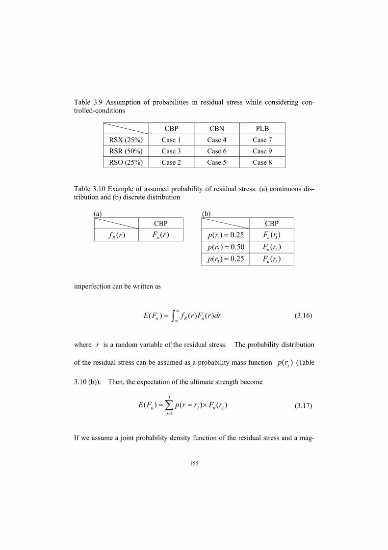
155

Table 3.9 Assumption of probabilities in residual stress while considering con-trolled-conditions

CBP CBN PLB

RSX (25%) Case 1 Case 4 Case 7

RSR (50%) Case 3 Case 6 Case 9

RSO (25%) Case 2 Case 5 Case 8

Table 3.10 Example of assumed probability of residual stress: (a) continuous dis-tribution and (b) discrete distribution

(a) (b)CBP CBP

)(rfR )(rFu 25.0)( 1 rp )( 1rFu

50.0)( 2 rp )( 2rFu

25.0)( 3 rp )( 3rFu

imperfection can be written as

drrFrfFE uRu )()()( (3.16)

where r is a random variable of the residual stress. The probability distribution

of the residual stress can be assumed as a probability mass function )( jrp (Table

3.10 (b)). Then, the expectation of the ultimate strength become

3

1

)()()(j

juju rFrrpFE (3.17)

If we assume a joint probability density function of the residual stress and a mag-

156

nitude of initial geometric imperfection as ),(, irf IR , the expectation of the ulti-

mate strength under the given shape of initial geometric imperfection can be ex-

pressed as

didrirfirFFE IRuu ),(),()( , (3.18)

Where i is a random variable of the magnitude of initial geometric imperfection.

If r and i are statistically independent, Eq. (3.18) becomes

didrifrfirFFE IRuu )()(),()( (3.19)

where )(rfR and )(ifI are the marginal probability density function of r and

i . Eq (3.19) can be expressed by discrete form as

m

j

n

kkjkjuu iiprrpirFFE )()(),()( (3.20)

From Eq. (3.16)~(3.20), we can derive the weighted average of the ultimate com-

pressive strength considering the uncertainties of residual stresses and initial

geometric imperfections.

157

Chapter 4

Validity of current design code ‘FHWA provisions’

AASHTO LRFD bridge design specification (2007) has general provisions for a

box girder section, However, due to limitations of applicability (e.g., long span,

many stiffeners), AASHTO LRFD bridge design specification recommend FHWA

provisions for the design of steel box-girder bridges proposed by Wolchuk and

Mayrbourl (1980). The provisions are based on the strut approach, which uses a

partial instead of entire cross-section for calculating the ultimate compressive

strength. The FHWA provisions have been widely used for over thirty years be-

cause the approach provides an opportunity to check the strength of chosen sec-

tions rapidly and to clearly determine structural behaviors such as column-type

buckling or plate-type buckling (Ziemian, 2010). However, how accurately the

provisions predict the ultimate compressive strength of a wide stiffened flange is

questionable, since the FHWA provisions were developed by using two indepen-

dent models (strut and flange plate) under certain assumptions. The provisions do

not use stiffened flanges.

In this chapter, background and history of the FHWA provisions are reviewed.

Subsequently, the FHWA provisions are accurately evaluated in terms of FEA re-

sults, and the FHWA provisions are compared to Eurocode3 and KHBDC-CSB in

158

terms of design philosophy. In addition, applicability of the FHWA provisions to

SM570 and HSB600 steel is evaluated.

159

4.1 Philosophy and basic assumptions

As explained in chapter 1, there are three approaches for analyzing stiffened

flanges in a box-girder. Of the three approaches, the strut approach has been used

in FHWA provisions. In this section, strut approach philosophy and some basic

assumptions are described.

Under in-plane compression, inelastic behaviors of stiffened flanges between

diaphragms (or transverse stiffeners) can be categorized into two major modes: (1)

column-type buckling, (2) plate-type buckling. The prior is defined as column-

like behavior and the latter is defined as plate-like behavior in Eurocode3. Phi-

losophy of the strut approach used in the FHWA provisions starts from the as-

sumption that behaviors of stiffened flanges are confined to only column-type

buckling and plate-type buckling. Thus, the strut approach is accompanied by

strength requirements of the stiffener to ensure that stiffener local buckling does

not occur before the above two modes. Two interpretations for the same stiffened

flanges are performed independently when considering the two modes. For the

column-like behavior, the stiffened flanges are considered a disconnected strut con-

sisting of a stiffener and an associated width of the plate as shown in Figs. 4.1(a)

and 4.2(a). The first assumption is that the longitudinal stiffeners have to be

equally spaced. If they are not equally spaced, the varied cross-section of the

struts lead to inconsistent strengths and one of the struts cannot be the representa-

tive strength of the stiffened flanges.

160

Fig. 4.1 Geometry for (a) column-like behavior and (b) plate-like behavior inflanges stiffened with open-type stiffeners under the strut approach

Fig. 4.2 Geometry for (a) column-like behavior and (b) plate-like behavior inflanges stiffened with closed-type stiffeners under the strut approach

The second assumption is that the function of diaphragms (transverse stiffeners) is

treated as simple rotationally free supports to the ends of longitudinal struts. Thus,

the strut can be analyzed as a simple column. However, for stiffened flanges with

closed-type stiffeners, the FHWA provisions do not clearly explain how to deter-

mine the w in Fig. 4.2(a) if the spacing of the closed-type stiffeners is wider than

two times of the width of stiffener.

For the plate-like behavior, the stiffened flanges are considered as disconnect-

ed unstiffened flanges between longitudinal stiffeners as shown in Figs. 4.1(b) and

4.2(b). The assumption is that the longitudinal stiffeners provide the condition of

simple supports to the unstiffened flanges. Thus, the plate-like behavior can be

analyzed easily as the flange.

w w

(a) (b)

w w

(a) (b)

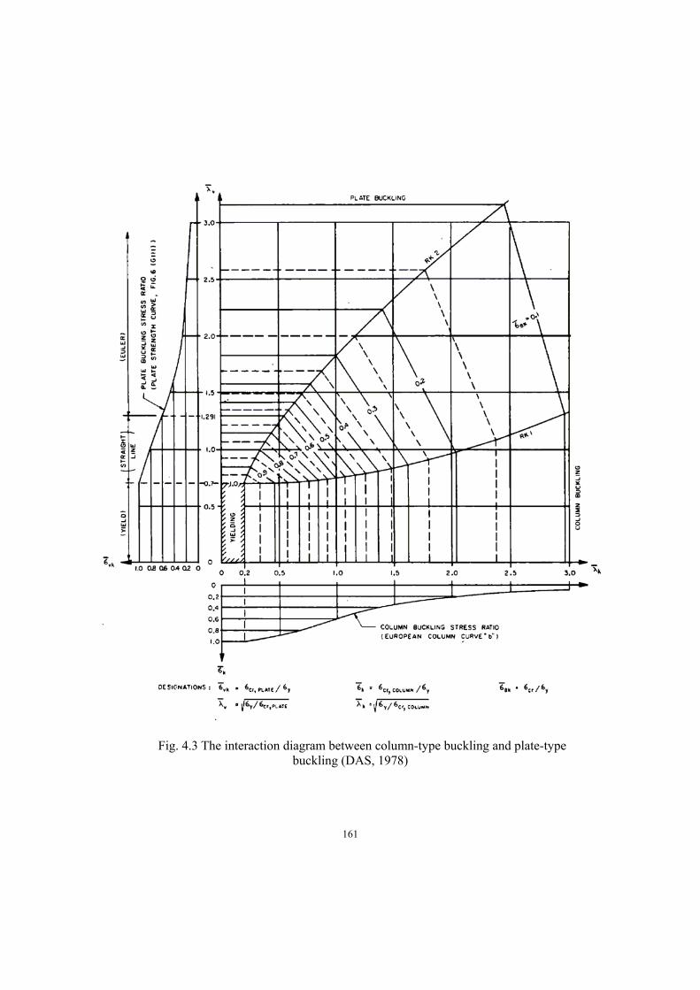
161

Fig. 4.3 The interaction diagram between column-type buckling and plate-typebuckling (DAS, 1978)

162

Fig. 4.4 The interaction diagram between column-type buckling and plate-typebuckling (FHWA, 1980)

The two strength curves can be derived independently from the two behaviors.

The ultimate compressive strengths are determined from these two curves. Such

an approach was suggested by Dwight and Little (1976). Das (1978) used the

interaction diagram for a box-girder design. The diagram was divided into three

behaviors as shown in Fig. 4.3. Namely, they were the column-like behavior, the

plate-like behavior, and the interaction of column-like and plate-like behaviors.

Later, Wolchuk and Mayrbourl (1980) proposed a simpler interaction diagram in a

FHWA-TS-80-205 report. The diagram is divided into the column-like behavior

163

and the plate-like behavior as shown in Fig. 4.4. This implies that the minimum

strength of both the column-like and the plate-like behaviors is regarded as the

ultimate strength.

The FHWA provisions considered three cases of initial geometric imperfec-

tions. For initial geometric imperfection of the column-like behavior, positive and

negative half sign curves were used. The maximum magnitude was L/500, and

the value was codified for the fabrication tolerance in FHWA provisions. Com-

pared to current design codes (AISC 2005; AASHTO LRFD 2012), which suggest

L/1000~L/1500, L/500 is more conservative. For the initial imperfection of the

plate-like behavior, the shape and maximum magnitude were assumed as a ripple

and w/1000, respectively. Compared with Bridge Welding Code (AWS 2002),

which suggest w/120, w/1000 is relatively very small.

Yield stresses of steel used in FHWA specifications were 250MPa and 350MPa.

Based on steel with a yield stress of 350MPa, the maximum of compressive residu-

al stress was 73MPa, which is a similar level in comparison to Fukumoto’s model

with 0.25Fy (87.5MPa) compressive residual stress. According to previous studies

(Grondin et al., 1999; Chou et al., 2006), influence of compressive residual stresses

on the ultimate compressive strength is significant. However, the influence of a

magnitude of initial imperfection is not. Thus, we can expect that the influence of

the imperfections of this study on the strengths is not different from an influence of

imperfections of the FHWA provisions on strengths.

164

4.2 Ultimate compressive strength by the interaction diagram

method

The parameters defined for the column-like and plate-like behaviors in the FHWA

provisions are described. From the parameters, the ultimate compressive strength

can be easily calculated by the interaction diagram method. To confine the be-

haviors of stiffened flanges only to column-type buckling and plate-type buckling,

strength requirements preventing premature buckling of stiffeners are applied to the

design practice.

In the FHWA provisions, only inelastic column-type buckling and inelastic

plate-type buckling behaviors of stiffened flanges in compression are defined. To

explain the behaviors, non-dimensional parameters are used. They are introduced

in Eq. (3.1). Rewriting the equations,

r

L

E

F

F

F y

cr

ycol 1

(4.1)

E

Ftw

F

F yd

cr

ypl 9.1

/ (4.2)

where crF is the elastic buckling strength of the strut or flange plate, w is the

stiffener spacing, dt is the thickness of the flange plate, L is the longitudinal

165

length of the stiffened flange or transverse stiffener spacing, and r is the radius of

gyration of the strut, which is calculated with respect to the neutral axis.

The two parameters are a function of material property and geometry of stiff-

ened flanges. From the parameters, normalized ultimate compressive stress uF

by the strut approach is defined as

),( plcoly

u fF

F (4.3)

where f is an implicit function of the slenderness parameters. yu FF / is

graphically shown in Fig. 4.4. The broken line in the figure denotes the division

line of the column-like behavior and the plate-like behavior. The ultimate com-

pressive strength in the column-like behavior is a function of col only. This can

be confirmed with the vertical lines in the interaction diagram. However, the ul-

timate compressive strength in the plate-like behavior is a function of both col

and pl . The inclined line explains the relations in the interaction diagram. If

each of the strength lines in the interaction diagram is extended without a division

line, we can obtain two independent strengths (inelastic plate-like and inelastic

column-like) for the given slenderness set. Of the two strengths, the smaller value

is consistent with the ultimate compressive strength suggested in the diagram.

From Eq. (4.3), ultimate capacity of stiffened flanges uP is computed as

166

fuu AFP (4.4)

where fA is the cross-sectional area of the flange and all longitudinal stiffeners.

In the FHWA provisions, limitations of geometry for open-shape stiffeners are

described in detail. However, for closed stiffeners, only the strength requirement

in which the strength of each plate element of the stiffeners shall not be less than

the strength of the stiffened flange is introduced. A notable item is that the

strength is expressed by a dimension of stress. The ultimate strength of a single

plate element is calculated with respect to the plate slenderness parameter as

65.0pl

yu FF (4.5a)

5.165.0 pl

])73.1(43.05.0[ 2 plyu FF (4.5b)

pl5.1

)20.082.0( plyu FF (4.5c)

The hypothetical models used in this study are checked by this equation, and no

violations occur.

167

4.3 Evaluation of ultimate compressive strength of stiffened

flanges by the FHWA provisions

The ultimate compressive strengths by the FHWA provisions are evaluated for the

six series of models in term of the FEA results. The six series defined in Table

2.4 are the thick (P03), the intermediate (P07) and the thin (P13) flanges, and the

short (C03), the intermediate (C07) and the long (C13) flanges. The ranges of the

slenderness parameters for the objective sections are described in Fig. 4.5.

Fig. 4.5 Investigated ranges of slenderness parameters

0.3 0.5 0.7 0.9 1.1 1.3 col

pl

0.3

0.5

0.7

0.9

1.1

1.3

Short(a1), (a2)

Intermediate(b1), (b2)

Long(c1), (c2)

Thick(A1), (A2)

Intermediate(B1), (B2)

Thin(C1), (C2)

168

For each section, the ultimate compressive strengths by the FEA results and those

by the FHWA provisions for all analysis cases (Table 2.6) are visualized in Figs.

4.6 and 4.7.

Figs. 4.6 (A1) through 4.6 (C2) show the ultimate compressive strengths of the

thick, the intermediate and the thin flanges with respect to col . Generally, the

FHWA provisions estimate the minimum strengths of FEA accurately in the force

control, except at large values of col . The provisions show the significant dif-

ference with strengths in the displacement control at all ranges of col . A similar

tendency occurs in Figs. 4.7 (a1) through 4.7 (c2), which show the ultimate com-

pressive strengths of the short, the intermediate and the long flanges with respect to

pl . Generally, the FHWA provisions estimate the minimum strengths of FEA

accurately in the force control, except the long (C13) flanges. However, the pro-

visions shows the significant difference with strengths in the displacement control

at all ranges of pl . Considering the diaphragm effect which is negligible in the

range of the practical design (under 30mm), the FHWA provisions are very appro-

priate for evaluation of the ultimate compressive strength of stiffened flange.

However, strengths in the displacement control seem to be overestimated compared

with the FHWA provisions and the proposed strength formula if the practical thick-

ness of the diaphragms is considered.

169

0

0.2

0.4

0.6

0.8

1

1.2

0.2 0.4 0.6 0.8 1 1.2 1.4

1. FC-CBP-RSX2. FC-CBP-RSO3. FC-CBP-RSR4. FC-CBN-RSX5. FC-CBN-RSO6. FC-CBN-RSR

7. FC-PBO-RSX8. FC-PBO-RSO9. FC-PBO-RSRElastic buckling strengthFHWA

Fu

/ Fy

col

(A1)

0

0.2

0.4

0.6

0.8

1

1.2

0.2 0.4 0.6 0.8 1 1.2 1.4

1. DC-CBP-RSX2. DC-CBP-RSO3. DC-CBP-RSR4. DC-CBN-RSX5. DC-CBN-RSO

6. DC-CBN-RSR7. DC-PBO-RSX8. DC-PBO-RSO9. DC-PBO-RSRFHWA

Fu

/ Fy

col

(A2)

0

0.2

0.4

0.6

0.8

1

1.2

0.2 0.4 0.6 0.8 1 1.2 1.4

1. FC-CBP-RSX2. FC-CBP-RSO3. FC-CBP-RSR4. FC-CBN-RSX5. FC-CBN-RSO6. FC-CBN-RSR

7. FC-PBO-RSX8. FC-PBO-RSO9. FC-PBO-RSRElastic buckling strengthFHWA

Fu

/ Fy

col

(B1)

0

0.2

0.4

0.6

0.8

1

1.2

0.2 0.4 0.6 0.8 1 1.2 1.4

1. DC-CBP-RSX2. DC-CBP-RSO3. DC-CBP-RSR4. DC-CBN-RSX5. DC-CBN-RSO

6. DC-CBN-RSR7. DC-PBO-RSX8. DC-PBO-RSO9. DC-PBO-RSRFHWA

Fu

/ Fy

col

(B2)

0

0.2

0.4

0.6

0.8

1

1.2

0.2 0.4 0.6 0.8 1 1.2 1.4

1. FC-CBP-RSX2. FC-CBP-RSO3. FC-CBP-RSR4. FC-CBN-RSX5. FC-CBN-RSO6. FC-CBN-RSR

7. FC-PBO-RSX8. FC-PBO-RSO9. FC-PBO-RSRElastic buckling strengthFHWA

Fu

/ Fy

col

(C1)

0

0.2

0.4

0.6

0.8

1

1.2

0.2 0.4 0.6 0.8 1 1.2 1.4

1. DC-CBP-RSX2. DC-CBP-RSO3. DC-CBP-RSR4. DC-CBN-RSX5. DC-CBN-RSO

6. DC-CBN-RSR7. DC-PBO-RSX8. DC-PBO-RSO9. DC-PBO-RSRFHWA

Fu

/ Fy

col

(C2)

Fig. 4.6 Comparison of FEA results with strengths by FHWA: Thick flanges in(A1) FC and (A2) DC, Intermediate flanges in (B1) FC and (B2) DC, Thin flanges

in (C1) FC and (C2) DC.

170

0

0.2

0.4

0.6

0.8

1

1.2

0.2 0.4 0.6 0.8 1 1.2 1.4

1. FC-CBP-RSX2. FC-CBP-RSO3. FC-CBP-RSR4. FC-CBN-RSX5. FC-CBN-RSO6. FC-CBN-RSR

7. FC-PBO-RSX8. FC-PBO-RSO9. FC-PBO-RSRElastic buckling strengthFHWA

Fu

/ Fy

pl

(a1)

0

0.2

0.4

0.6

0.8

1

1.2

0.2 0.4 0.6 0.8 1 1.2 1.4

1. DC-CBP-RSX2. DC-CBP-RSO3. DC-CBP-RSR4. DC-CBN-RSX5. DC-CBN-RSO

6. DC-CBN-RSR7. DC-PBO-RSX8. DC-PBO-RSO9. DC-PBO-RSRFHWA

Fu

/ Fy

pl

(a2)

0

0.2

0.4

0.6

0.8

1

1.2

0.2 0.4 0.6 0.8 1 1.2 1.4

1. FC-CBP-RSX2. FC-CBP-RSO3. FC-CBP-RSR4. FC-CBN-RSX5. FC-CBN-RSO6. FC-CBN-RSR

7. FC-PBO-RSX8. FC-PBO-RSO9. FC-PBO-RSRElastic buckling strengthFHWA

Fu

/ Fy

pl

(b1)

0

0.2

0.4

0.6

0.8

1

1.2

0.2 0.4 0.6 0.8 1 1.2 1.4

1. DC-CBP-RSX2. DC-CBP-RSO3. DC-CBP-RSR4. DC-CBN-RSX5. DC-CBN-RSO

6. DC-CBN-RSR7. DC-PBO-RSX8. DC-PBO-RSO9. DC-PBO-RSRFHWA

Fu

/ Fy

pl

(b2)

0

0.2

0.4

0.6

0.8

1

1.2

0.2 0.4 0.6 0.8 1 1.2 1.4

1. FC-CBP-RSX2. FC-CBP-RSO3. FC-CBP-RSR4. FC-CBN-RSX5. FC-CBN-RSO6. FC-CBN-RSR

7. FC-PBO-RSX8. FC-PBO-RSO9. FC-PBO-RSRElastic buckling strengthFHWA

Fu

/ Fy

pl

(c1)

0

0.2

0.4

0.6

0.8

1

1.2

0.2 0.4 0.6 0.8 1 1.2 1.4

1. DC-CBP-RSX2. DC-CBP-RSO3. DC-CBP-RSR4. DC-CBN-RSX5. DC-CBN-RSO

6. DC-CBN-RSR7. DC-PBO-RSX8. DC-PBO-RSO9. DC-PBO-RSRFHWA

Fu /

Fy

pl

(c2)

Fig. 4.7 Comparison of FEA results with strengths by FHWA: Short flanges in(a1) FC and (a2) DC, Intermediate flanges in (b1) FC and (b2) DC, Long flanges in

(c1) FC and (c2) DC.

171

At large values of col in Figs. 4.6 (A1), (B1) and (C1), the FHWA provisions

shows conservative strengths compared to FEA strengths. The results are also

clearly shown in Fig. 4.6(c1). These results are consistent with Shin et al. (2013),

which explained that safety factors for the ultimate strength in FHWA provisions

increase with the increase of col . This is related with design philosophy that

column-type buckling is regarded as more detrimental behavior compared to plate-

type buckling, since the column-type buckling occurs abruptly, but the plate-type

buckling occurs gradually. Actually, this fact is not major concern because the

slender sections in longitudinal direction are rarely used in practical design of steel

box-girder.

Strengths of the FHWA provisions are compared with those of Eurocode3 (EN

1993-1-5, 2004), KHBDC-CSB (MLIT, 2015), the proposed formula and strength

formula by DC (Figs. 4.6 and 4.7).

Fig. 4.8 shows the ultimate compressive strengths of the thick, intermediate

and thin flanges. The FEA results in the force control and displacement control

are also plotted in one graph. The FEA results show that large variation of ulti-

mate compressive strengths can occur depending on the control methodologies.

The FHWA provisions is very close to proposed formula. In the FHWA provi-

sions and proposed formulas, strong inclination and mild inclination denote the

column-like behavior and the plate-like behavior, respectively. The FHWA provi-

sions and the proposed formula show the column-like behavior in the thick flanges,

172

the plate-like behavior in the thin flanges, and both the column-like and plate-like

behaviors in the intermediate flanges. Generally, Eurocode3 shows strong incli-

nation in Fig. 4.8(a), 4.8(b) and 4.8(c). Thus, the column-type buckling is more

dominant in Eurocode3 in comparison to the FHWA provisions or proposed for-

mula. In the case of Eurocode3, two reduction factors are sequentially applied to

the stiffened flanges with U-ribs. The first reduction factor is for all sub-panel

elements to account for local plate buckling. The second reduction factor is for

the stiffened flange to account for overall (global) buckling between column-like

behavior and plate-like behavior. The overall reduction factor is very close to that

of the column-like behavior due to the low aspect ratio of wide stiffened flanges.

Thus, most behaviors are governed by the overall column-type buckling excluding

the very thin and short components (elements). KHBDC-CSB shows the plate-

like behaviors (mild inclination) in the all flanges (thick, intermediate and thin),

because the equation of KHBDC-CSB was derived based on the plate slenderness

parameter. KHBDC-CSB considered the column-like behaviors slightly using

safety concept.

Comparing Eurocode3 with the FEA results in Fig. 4.8(C), the strength by

Eurocode3 goes up to average value of FEA in DC at 3.0col . Similarly,

comparing the KHBDC-CSB with FEA results in Fig. 4.8(A), the strength by

KHBDC-CSB goes up to average value of FEA in DC at 3.1col . From the

results, we can deduce that upper limit of strengths by Eurocode3 and KHBDC is

173

0.2

0.4

0.6

0.8

1

1.2

0.2 0.4 0.6 0.8 1 1.2 1.4

FHWAEurocodeKHBDC-CSBFC formula (Proposed)DC formulaFEA in FCFEA in DC

Fu

/ Fy

col

(A)

0.2

0.4

0.6

0.8

1

1.2

0.2 0.4 0.6 0.8 1 1.2 1.4

FHWAEurocodeKHBDC-CSBFC formula (Proposed)DC formulaFEA in FCFEA in DC

Fu

/ Fy

col

(B)

0.2

0.4

0.6

0.8

1

1.2

0.2 0.4 0.6 0.8 1 1.2 1.4

FHWAEurocodeKHBDC-CSBFC formula (Proposed)

DC formulaFEA in FCFEA in DC

Fu

/ Fy

col

(C)

col= 0.8

Fig. 4.8 Strength comparison of FHWA with Eurocode3, KHBDC-CSB, pro-posed formulas and FEA: (A) Thick flanges (B) Intermediate flanges (C) Thin

flanges

174

0.2

0.4

0.6

0.8

1

1.2

0.2 0.4 0.6 0.8 1 1.2 1.4

FHWAEurocodeKHBDC-CSBFC formula (Proposed)DC formulaFEA in FCFEA in DC

Fu

/ Fy

pl

(a)

0.2

0.4

0.6

0.8

1

1.2

0.2 0.4 0.6 0.8 1 1.2 1.4

FHWAEurocodeKHBDC-CSBFC formula (Proposed)

DC formulaFEA in FCFEA in DC

Fu

/ Fy

pl

(b)

0.2

0.4

0.6

0.8

1

1.2

0.2 0.4 0.6 0.8 1 1.2 1.4

FHWAEurocodeKHBDC-CSB

FC formula (Proposed)DC formulaFEA in FCFEA in DC

Fu

/ Fy

pl

(c)

Fig. 4.9 Strength comparison of FHWA with Eurocode3, KHBDC-CSB, pro-posed formulas and FEA: (a) Short flanges (b) Intermediate flanges (b) Long

flanges

175

the average strength of FEA in DC.

Fig. 4.9 shows the ultimate compressive strengths of short, intermediate and

long flanges. In the strength curves with respect to pl , flat inclination and de-

creasing line denote the column-like behavior and the plate-like behavior, respec-

tively. The FHWA provisions, Eurocode3 and the proposed formula shows simi-

lar patterns for flat inclinations with widened ranges as the stiffened flanges be-

come long as shown in Figs. 4.9(a), 4.9(b) and 4.9(c). However, Eurocode3

shows the strong column-like behaviors as the longitudinal length of the stiffened

flanges increase in comparison to the FHWA provisions and the proposed formulas.

For all flanges (thick, intermediate and thin) in Fig 4.9, KHBDC-CSB shows the

plate-like behavior due to design philosophy.

Figs. 4.10~4.13 show interaction diagrams of the proposed strength formula

and current design codes. The ranges of the slenderness parameters are from 0.3

to 1.2 at col and 0.3 to 1.2 at pl . Generally, as the interaction curve is closer

to vertical line, the more dominant the column-like behavior is. Similarly, as the

interaction curve is closer to horizontal line, the more dominant the plate-like be-

havior is. Eurocode3 shows dominant column-like behavior, but KHBDC shows

dominant plate-like behavior. The FHWA provisions and the proposed strength

formula show both the plate-like behavior and the column-like behavior. In two-

dimensional interaction diagram of the FHWA provisions and proposed strength

formulas, the upper area and lower area of the division line denote plate-like be-

176

havior and column-like behavior, respectively. The design philosophies of the

proposed strength formula and current design codes are very clear in the 3D

strength surface.

Lambda C

Lam

bda

P

0.2 0.4 0.6 0.8 1 1.20.2

0.4

0.6

0.8

1

1.2

Fu/Fy=0.9

0.8

0.7

0.6

0.5

0.30.6

0.91.2

0.30.6

0.91.2

0.2

0.4

0.6

0.8

1

Lambda CLambda P

Fu/F

y

Fig. 4.10 Two dimensional and three dimensional interaction diagram ofproposed strength formula (FC)

Lambda C

Lam

bda

P

0.2 0.4 0.6 0.8 1 1.20.2

0.4

0.6

0.8

1

1.2

Fu/Fy = 0.9

0.8

0.7

0.6

0.5

0.30.6

0.91.2

0.30.6

0.91.2

0.2

0.4

0.6

0.8

1

Lambda CLambda P

Fu/F

y

Fig. 4.11 Two dimensional and three dimensional interaction diagram ofFHWA provisions

177

Lambda C

Lam

bda

P

0.2 0.4 0.6 0.8 1 1.20.2

0.4

0.6

0.8

1

1.2

Fu/Fy=0.9 0.8 0.7 0.6 0.5

0.30.6

0.91.2

0.30.6

0.91.2

0.2

0.4

0.6

0.8

1

Lambda CLambda P

Fu/F

y

Fig. 4.12 Two dimensional and three dimensional interaction diagrams ofEurocode3

Lambda C

Lam

bda

P

0.2 0.4 0.6 0.8 1 1.20.2

0.4

0.6

0.8

1

1.2

Fu/Fy=0.9

0.8

0.7

0.6

0.5

0.30.6

0.91.2

0.30.6

0.91.2

0.2

0.4

0.6

0.8

1

Lambda CLambda P

Fu/F

y

Fig. 4.13 Two dimensional and three dimensional interaction diagrams ofKHBDC-CSB

178

4.4 Applicability of the FHWA provisions to HSB600 steel and

SM570 steel

The FHWA provisions were established for two grades of steel with yield strengths

of 250MPa and 350MPa. Recently, high-performance steels (HPS) have been

developed. Especially, HSB600 steel, whose yield stress reaches 450MPa, is

widely used in the steel box-girder design. However, whether the FHWA provi-

sions are applicable to HSB600 steel was not determined until Shin (2013). The

study showed that when HPS was used, the ultimate compressive strengths by the

FHWA provisions were on the conservative side in comparison to their FEA solu-

tions. In addition, the study pointed out that the FHWA provisions have a larger

safety margin at high values of col in comparison to conventional steel. Thus,

the conservative tendency of the FHWA provisions increases as the yield stresses of

steel increase. However, FEA in Shin et al. (2013) were performed in the dis-

placement control. As already demonstrated in this study, the FHWA provisions

accurately estimate the ultimate compressive strength in the force control. If the

FHWA provisions are viewed in the force control, the conservative tendency may

disappear. Thus, the applicability of the FHWA provisions to HSB600 steel in re-

evaluated in the context of the force control. Conventional steel SM570 which

have the 450MPa yield stress also analyzed.

The material properties and stress-strain relations are assumed (Shin, 2012)

179

and are summarized in Table 4.1 and Fig. 4.14 and 4.15. The ultimate compres-

sive strengths of the stiffened flanges with U-ribs are analyzed considering initial

imperfection and residual stresses used in the minimum strength cases in chapter 3.

When the RSR (considered with recovery) case occurs in the minimum strength

cases, the case is excluded and an alternative case is selected for evaluation of

strengths in conservative side.

Figs. 4.16 show a comparison of strengths from the FHWA provisions, the

proposed strength formula and the FEA results. The FHWA provisions and the

proposed formula have a high accuracy for HSB600 and SM570 steels. In addi-

tion, the conservative tendency is not observed in the context of the force control.

Thus, the FHWA provisions are still applicable to the steels that have 450MPa yield

stress.

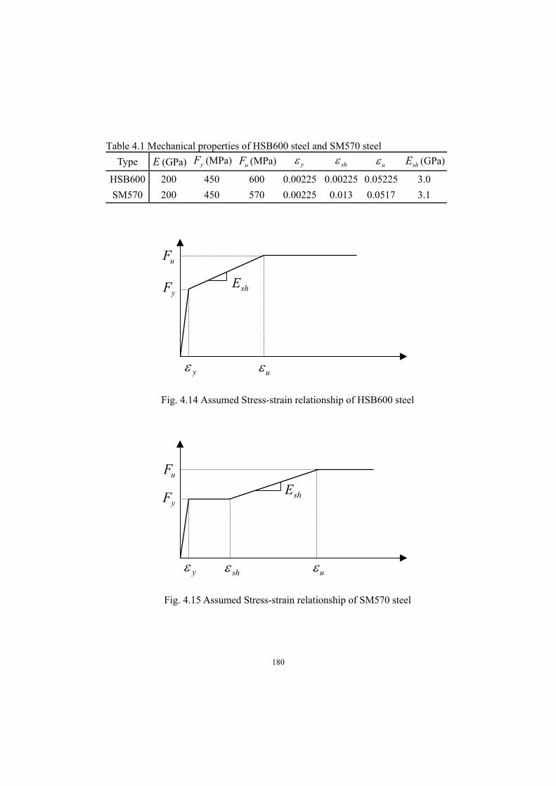
180

Table 4.1 Mechanical properties of HSB600 steel and SM570 steel

Type E (GPa) yF (MPa) uF (MPa) y sh u shE (GPa)

HSB600 200 450 600 0.00225 0.00225 0.05225 3.0

SM570 200 450 570 0.00225 0.013 0.0517 3.1

Fig. 4.14 Assumed Stress-strain relationship of HSB600 steel

Fig. 4.15 Assumed Stress-strain relationship of SM570 steel

shEyF

uF

y ush

shE

uF

yF

y u

181

0

0.2

0.4

0.6

0.8

1

1.2

0.2 0.4 0.6 0.8 1 1.2 1.4

FEA by SM570 steelFEA by HSB600 steelFHWAProposed stength formula (FC)

Fu

/ Fy

col

(A)

0

0.2

0.4

0.6

0.8

1

1.2

0.2 0.4 0.6 0.8 1 1.2 1.4

FEA by SM570 steelFEA by HSB600 steelFHWAProposed stength formula (FC)

Fu

/ Fy

col

(B)

0

0.2

0.4

0.6

0.8

1

1.2

0.2 0.4 0.6 0.8 1 1.2 1.4

FEA by SM570 steelFEA by HSB600 steelFHWAProposed stength formula (FC)

Fu

/ Fy

col

(C)

Fig. 4.16 Applicability of FHWA provisions and proposed formulas to HSB600 andSM570 steel: (a) Thick flanges, (b) Intermediate flanges, (c) Thin flanges

182

Chapter 5

Conclusions and further study

Conclusions

This study proposes a method to evaluate the in-plane ultimate compressive

strength of flanges stiffened with U-ribs in a wide steel box-girder. The stiffened

flanges with U-ribs are separated from the box-girder and modeled by finite ele-

ments with idealized boundary conditions. Generally, the stiffened flanges be-

tween diaphragms are designed to behave as if simple support conditions were

applied. If the diaphragms are stiff (thick) enough, loaded edges of the stiffened

flanges have the same displacement in longitudinal direction. This condition can

be analyzed by displacement control. However, if the diaphragms are flexible

(thin) enough, all parts of the loaded edge of the stiffened flanges will have differ-

ent displacements in the longitudinal direction. This condition has to be analyzed

by force control. Thus, the ultimate compressive strength of the stiffened flanges

with U-ribs are evaluated considering effects of the bending stiffness of the dia-

phragms on in-plane behaviors of the stiffened flanges in this study. The results

reveal that the load-displacement curves of the stiffened flanges considering the

diaphragms do not deviate significantly from the load displacement curve in the

force control while thickness of the diaphragms is increased to 40mm. In addition,

183

the longitudinal displacements at the loaded edges of the stiffened flanges consid-

ering the diaphragms do not deviate significantly from the longitudinal displace-

ments in the force control, and the differences between the displacements in the

force control and the displacement control does not be narrowed while thickness of

the diaphragms is increased to 40mm. As results, it is confirmed that the force

control is more appropriate than the displacement control under the practical thick-

ness, which is less than 30mm, of the diaphragms. Based on the strengths in the

force control, the strength formula is proposed with considering the inelastic buck-

ling behaviors. The current design codes, the FHWA provisions, Eurocode3 and

KHBDC-CSB, are evaluated in terms of the proposed strength formula. The

comparative study reveals that the strengths from the FHWA provisions are nearly

the same as the strengths from the proposed strength formula.

This study considers three cases of the initial geometric imperfections (posi-

tive column-type buckling, negative column-type buckling and plate-type buck-

ling) and three cases of the residual stresses (‘not-considered’, ‘simply-considered’

and ‘considered with recovery’). Thus, total nine combinations of the imperfec-

tions are considered to reflect the most critical condition in this study. From the

conservative approach, the minimum value from the nine analysis cases is deter-

mined as the ultimate compressive strength. The arithmetic mean and standard

deviation from the strengths in the nine analysis cases can be interpreted as the

weighted average and standard deviation based on an assumption that nine analysis

cases have same probability. The methodology to consider a residual stress and a

184

magnitude of initial geometric imperfection as random variables is also introduced.

In terms of the details, influences of the slenderness parameter, the initial

geometric imperfection and the residual stresses on the ultimate compressive

strength of stiffened flanges are analyzed. The ultimate compressive strength

versus the plate slenderness parameter shows that a certain level at the column-like

behavior is maintained but decrease rapidly at the plate-like behavior. However,

the ultimate compressive strength versus the column slenderness parameter shows

that the strength linearly decreases while the column slenderness parameter in-

creases.

In the case of the initial geometric imperfections, when the residual stresses

are considered, the influence of the initial geometric imperfection of the plate-type

buckling shape on the ultimate compressive strength of stiffened flanges is signifi-

cant if the fracture mode is the plate-type buckling. The maximum reduction is

approximately 10% compared to the other initial imperfection shapes. However,

the influence of the initial imperfection shapes is not significant if the fracture

mode is the column-type buckling.

In the case of the residual stresses, if considered, the ultimate compressive

strength of stiffened flange roughly decreases by 0~40% in the force control and

0~25% in the displacement control compared to the not-considered cases. Con-

sidering that the magnitude of compressive residual stress in this study is 25% of Fy,

a reduction effect is significant in the force control due to a relatively weak con-

straint in comparison to the displacement control. This study shows that the in-

185

fluence of the residual stresses is generally more significant than the influence of

the initial imperfection shapes in the inelastic buckling behavior of the stiffened

flanges. This is consistent with the results of classical stiffened flanges.

In the middle of evaluating the influence of the shapes of initial geometric

imperfection, an unexpected deflection behavior occurs in the stiffened flanges

with U-ribs. A direction of the out-of-plane deflection in the stiffened flanges is

changed before reaching the ultimate compressive strength. The yielding of the

flanges at turning points of the deflection is a mechanism that contributes to stiff-

ness loss of the stiffened flanges and leads to changing the direction of displace-

ment. This phenomenon is called snap-through like phenomenon in this study.

Of the models experiencing snap-through like phenomenon, the change of global

configuration mode occurs in the force control. However, the change of global

configuration mode does not occur in the displacement control due to the property

of an additional constraint effect. This phenomenon leads to an increase in the

ultimate compressive strength, except in the case of very short plates.

The Federal Highway Administration provisions is reviewed and evaluated in

terms of finite element analysis solution. How accurately the provisions predict

the ultimate compressive strength of a wide stiffened flange is questionable be-

cause the provisions were developed without using the stiffened flanges. How-

ever, two independent models (strut and flange plate) are used under certain as-

sumptions. Nevertheless, the comparison of FEA solutions with strengths by the

FHWA provisions shows that the FHWA provisions accurately estimate the mini-

186

mum strengths of FEA solutions in the force control. In terms of the design phi-

losophies, Eurocode3 shows dominant column-like behavior, but KHBDC-CSB

shows dominant plate-like behavior. The FHWA provisions and the proposed

strength formula show both the plate-like behavior and the column-like behavior

harmoniously. The FHWA provisions and the proposed strength formula show

high accuracy for HSB600 and SM570 steels. Thus, the FHWA provisions and

the proposed strength formula are still applicable to HSB600 and SM570 steels.

It is believed that the force control is more appropriate compared to the dis-

placement control for evaluation of the ultimate compressive strength of stiffened

flanges with U-ribs in a wide steel box-girder. Therefore, this study recommends

the proposed strength formula or the FHWA provisions. Either way, the ultimate

compressive strengths are almost same.

187

Further study

Validity of force control in full box-girder

This studies show that the force control is more appropriate than the displacement

control for evaluation of the ultimate compressive strength of stiffened flanges with

U-ribs. The validity of the force control is confirmed in one-bay models consist-

ing of stiffened flanges and two diaphragms. However, it is not verified that the

force control is more appropriate than the displacement control for evaluation of

the ultimate flexural strength of a whole box-girder. This issue is recommended.

Effective width of a flange for constituting a strut with a closed stiff-

ener

According to the strut approach, stiffened flanges are considered as disconnected

struts consisting of a stiffener and an associated width of the flange for the column-

like behavior. In the case of an open type stiffener, there is no problem to deter-

mine the associated width of the flange. However, if closed-type stiffeners are

used in stiffened flanges and a spacing of the closed-type stiffeners is wider than

two times of the width of stiffener, the widths of the flanges at the inner and outer

sides of the U-ribs are different for each other. Thus, we are not sure what ‘an

associated width’ of flanges for constituting the strut should be. Research on this

issue is recommended.

188

REFERENCES

ABAQUS Inc. (2011), ABAQUS standard user’s manual. Ver. 6.11.

American Association of State Highway and Transportation Officials (1998).AASHTO LRFD Bridge design specifications. Washington, DC.

American Association of State Highway and Transportation Officials (2007).AASHTO LRFD Bridge design specifications. 4th ed. Washington, DC.

American Institute of Steel Construction (2005), Steel construction manual.

Ang, A. H. S., & Tang, W. H. (2007). Probability Concepts in Engineering:Emphasis on Applications to Civil and Environmental Engineering (v. 1).

ANSI/AASHTO/AWS D1.5-96 (2002), Bridge welding code, A joint publica-tion of the American Association of State Highway and Transportation offi-cials and the American Welding Society, Washington DC.

Bathe K. Finite element procedures (1996). Englewood Cliffs (NJ), PrenticeHall.

Bedair, O. K. (1998). A contribution to the stability of stiffened plates underuniform compression. Computers & structures, 66(5), 535-570.

Chen, W. F., & Han, D. J. (1988). Plasticity for structural engineers. SpringerScience & Business Media.

Chen, Q., (1993) Bending strength of longitudinally stiffened steel cylinders.Structural Engineering Report No. 192, Department of Civil and Environ-mental Engineering, University of Alberta, Edmonton.

189

Chen, S.-J., Yang, K.-C., (2002) “Inelastic behavior of orthotropic steel deckstiffened by U-shaped stiffeners.” Thin-Walled Structures 40, pp.537-553.

Cho, E. Y., & Shin, D. K. (2010). Flexural Behavior of Composite HSB I-Girders in Positive Moment. Journal of Korean Society of Steel Construction,22(4), 377-388.

Chou C.C., Uang C.M., Seible F., (2006) “Experimental evaluation of com-pressive behavior of orthotropic steel plates for the new San Francisco-Oakland bay bridge.” Journal of Bridge Engineering, Vol. 11, No. 2, ASCE,pp.140-150.

Crisfield, M.A., (1981) fast incremental/iterative solution procedure that han-dles snap-through. Computer and structures, 13:55-62.

Crisfield, M.A., (1997) Non-linear Finite Element Analysis of Solids andStructures. JOHN WILEY & SONS, New York.

De Borst, R., Crisfield, M. A., Remmers, J. J., & Verhoosel, C. V. (2012).Nonlinear finite element analysis of solids and structures. John Wiley & Sons.

EN1993-1-5 (2004), EUROCODE3 Design of steel structures Part 1.5 Platedstructural elements.

Ellobody, E. (2014). Finite Element Analysis and Design of Steel and Steel–Concrete Composite Bridges. Butterworth-Heinemann.

Forde, B.W.R. & Sttemer, S.F. (1987), Improved arc length orthogonalitymethods for nonlinear finite element analysis, Computers & Structures,27:625-630.

Fukumoto Y., Usami T., Okamoto Y. (1974), “Ultimate compressive strengthof stiffenedplates”, Proc., Specialty Conf. on Metal Bridge, St. Louis, MO.

Flügge (1962), W. Handbook of Engineering Mechanics, McGraw-Hill, NewYork.

190

Fried, I.(1984), Orthogonal trajectory accession to the nonlinear equilibriumcurves, Comp. Meth. Appl. Mech. & Engng. 47:283-289.

Ghavami K, Khedmati MR. (2006), Numerical and experimental investiga-tions on the compression behaviour of stiffened plates. Journal of Construc-tional Steel Research, 62:1087–100.

Grondin, G. Y., Chen Q., Elwi, A.E. and Cheng, J.J.R. (1998), Stiffened SteelPlates under Compression and Bending, Journal of Constructional Steel Re-search, Vol. 45, No.2, pp. 235-148.

Grondin, G.Y., Elwi, A.E., Cheng, J.J.R. (1999), Buckling of stiffened plates-aparameteric study, Journal of Constructional Steel Research, Vol. 50, pp. 151-175.

Grimes, R.G., Lewis, J.G., Simom, H.D. (1994), A shifted block Lanczos algo-rithm for solving sparse symmetric generalized eigenproblems. SIAM Journalof Matrix Analysis and Applications, 15(1), 228-272.

Hu, S.Z. (1993), A finite element assessment of the buckling strength equa-tions of stiffened plates, In The Ship Structures Symposium ’93, Arlinton, VA,The Ship Structures Committee, pp.J1-J10.

Hill, R. (1998), The mathematical theory of plasticity, oxford UniversityPress, London.

Hughes, T. J. R., Winget, J. (1980), Finite rotation effect in numerical inte-gration of rate constitutive equation arising in large-deformation analysis. Int.J. for Numerical Methods in Engineering, 15:1862-1867.

Johnston, B.G., ed (1976). Structural Stability Research Council Guide toStability Design Criteria for Metal Structures, Third edition. John Wiley &Sons, New York.

James M, Gere.(2001), Mechanics of Materials, 5th ed., BROOKS/COLE.

191

Japan Road Association (2002), Specification for highway bridges: Part I,Tokyo.

Khludnev, A.M., Sokolowski, J. (1998), On solvability of boundary valueproblems in elasto-plasticity. Control Cybernet. 27, 311-330.

Kim, N.H. (2014), Introduction to Nonlinear Finite Element Analysis,Springer.

Lanczos, C. (1950), An iteration method for the solution of the eigenvalueproblem of linear differential and integral operators, Journal of Research ofthe national Bureau of Standards, Vol. 45, No. 4, pp. 255-282.

Little G. H., (1976), “Stiffened Steel Compression Panels - Theoretical FailureAnalysis.” The Structural Engineering, Vol. 54, No. 12, December, pp. 489-500.

MANDA, A., & NAKAMURA, S. (2010). Progressive Collapse Analysis ofSteel Truss Bridges. Strain, 2, 2-850.

Mikami I, Niwa K. (1996) Ultimate compressive strength of orthogonallystiffened steel plates. Journal of Structural Engineering, ASCE, 122(6):674–82.

Massonet, C.,and Maquoi, R.(1973), “New theory and tests on the ultimatestrength of stiffened box girders.” In Steel box girder bridges, Institution ofcivil engineering, London, 131-144.

McMeeking. R.M., and Rice. J.R. (1975), ‘Finite element formulation forproblems of large elastic-plastic deformation’, Int. J. Solids Structures, 11:601-616.

Ministry of Land, Infrastructure and Transport (2012), Korea Highway BridgeDesign Code.

192

Ministry of Land, Infrastructure and Transport, Super Long Span BridgeR&D Center (2015), Korea Highway Bridge Design Code - Cable Supportedbridge specification (KHBDC-CSB), Ver.16.1

PETROS P. XANTHAKOS.(1994), Theory and design of bridges, JOHNWILEY&SONS, New York, pp.465.

Ramm, E. (1981), Strategies for tracing the non-linear response near limit-points, Non-linear Finite element Analysis in structural Mechanics, ed. W.Wunderlich, Springer-Verlag, Berlin, pp. 63-89.

Ramm, E. (1982), The Riks/Wempner approach-an extension of the displace-ment control method in non-linear analysis, Non-linear ComputationalMechaics, de. E. Hilton, E. et al., Pineridge, Swansea, pp. 63-86.

Riks, E. (1972), The application of Newton’s method to the problem of elasticstability, J. Appl. Mech., 39: 1060-1066.

Riks, E. (1979), An incremental approach to the solution of snapping andbuckling problem, International Journal of Solids and Structures. 15: 529-551.

Ross, Sheldon M. (2006). A First Course In Probability 7th ed., Prentice Hall,NJ

Shin, D.K., Le, V.A., Kim, K. (2013), “In-plane ultimate compressivestrengths of HPS deck panel system stiffened with U-shaped ribs.” Thin-Walled Structures 63, pp.70-81.

Sheikh, I.A., Grondin G.Y. and Elwi A.E. (2001), Stiffener Tripping in Stiff-ened Steel Plates, Structural Engineering Report No. 236, Department of Civiland Environmental Engineering, University of Alberta.

Sheikh I.A., Grondin G.Y., Elwi A.E. (2002), “Stiffened steel plates underuniaxial compression” Journal of Constructional Steel Research.

193

Simo, J.C., Taylor, R.L. (1985), Consistent tangent operator for rate-dependent elastoplasticity. Computational Method in Applied Mechanics andEngineering.

Szilard, R. (2004). Theories and applications of plate analysis: classical nu-merical and engineering methods. John Wiley & Sons.

Wang E.C.L., Gondin G.Y., Elwi A.E. (2006), Interaction Buckling Failure ofStiffened Steel Plates, Structural Engineering Report No. 264, Department ofCivil and Environmental Engineering, University of Alberta.

Wempner, G.A. (1971), Discrete approximation related to nonlinear theoriesof solids. International Journal of Solids and Structures, 7:1571-1599.

Wolchuck, R., Mayrbourl, R.M. (1980), “Proposed Design Specification forSteel Box Girder Bridges”, Report No. FHWA-TS-80-205, Federal HighwayAdministraion, Washington, D.C.

Ziemian, R.D. (2010), Guide to Stability Design Criteria for Metal Structures,Sixth edition. John Wiley & Sons, New Jersey.

194

APPENDIX A. Ultimate compressive strength of flange stiffened

with U-ribs in Eurocode3 (EN 1993-1-5)

Two methods for evaluation of the ultimate compressive strength of stiffened

flanges with U-ribs are presented in EN 1993-1-5 of Eurocode 3. One is ‘effec-

tive section method’ which calculates a portion of cross-sectional area withstanding

up to the yield stress, and the other is ‘reduced stress method’ based on the gross

cross-section but with a reduced allowable stress limit. The former method take

account of the beneficial shedding of loads from overstressed panels, so EN 1993-

1-5 recommends it for greatest structural economy. The ultimate compressive

strength by effective section method in EN 1993-1-5 shall be written as

yeffcu FAP , (A.1)

where effcA , is an effective section considering an overall reduction (sub-panel

buckling and global buckling of the stiffened flanges), and calculated as

tbAA effedgeloceffcceffc ,,,, (A.2)

tbAAc

loccloceffslloceffc ,,,, (A.3)

where effslA , is the sum of the effective cross-sectional area of all the longitudinal

195

stiffeners, tbc

loccloc , is the effective-cross sectional area of all the sub-panels

(reduced for local plate buckling), except for the effective part of sub-panels which

are supported by a web or a flange plate ( tb effedge, ), c the reduction factor

for global buckling of the stiffened panel ignoring local buckling of sub-panels.

The reduction factor for global buckling c is determined from an empirical in-

terpolation between the reduction factors for the column-like buckling and for the

overall stiffened plate buckling.

ccc )2()( (A.4)

1/ ,, ccrpcr (A.5)

Where is the reduction factor for overall stiffened plate buckling, c reduc-

tion factor for the column-type buckling, pcr , and ccr , are elastic buckling

stress for the plate-type buckling and column-type buckling, respectively.

As shown in Eq. (A.2) ~ Eq. (A.5), the effective area is obtained mainly by re-

ducing the gross area in two steps. First, an effective area is derived for the sub-

panels and any slender closed stiffeners to account for local buckling. Second, a

reduction factor for global buckling of the whole stiffened panel is determined.

When viewed from first step, EN 1993-1-5 considers stiffener local plate buckling

whereas FHWA prevent it, but viewed from second step both codes consider the

196

plate-like behavior and column-like behavior, simultaneously.

197

국문초록

본 연구에서는 U리브로 보강된 광폭 강박스거더 플랜지의 극한 압축강

도를 평가하는 방법을 제안한다. 박스거더가 휨 또는 압축력을 받을 때,

박스거더의 상부플랜지나 하부플랜지는 면내 압축상태에 놓이게 된다.

만약 웹과 같은 다른 부재들이 충분한 강성을 가지고 있다면, 박스거더

의 극한휨강도는 상부플랜지 또는 하부플랜지의 극한압축강도에 의해서

지배된다. 이러한 이유로 본 연구에서는 보강판의 극한압축강도 평가를

수행하였다. 이를 위해, U리브로 보강된 판을 박스거더에서 분리한 후,

적절한 경계조건을 적용하여 모델링하였다.

일반적으로, 보강판은 다이아프램 사이에서 단순경계조건으로 거동

하도록 설계된다. 만약 다이아프램의 두께가 상당해서 면외 휨강성이 충

분하다면, 보강판에서 하중이 재하되는 부분의 면내 변위는 모두 동일하

게 발생할 것이다. 이 경우는, 변위제어법으로 해석할 수 있다. 그러나

다이아프램의 두께가 얇아서 면외 휨강성이 충분하지 않다면, 보강판에

서 하중이 재하되는 부분의 면내 변위는 모두 다르게 발생할 것이다. 이

경우는, 하중제어법으로 해석해야 한다. 본 연구에서는 다이아프램의 면

외 휨강성이 보강판의 면내 거동에 미치는 영향을 분석하여 U리브로 보

강된 플랜지의 극한압축강도를 평가하였다. 본 연구에는 실제 설계에서

198

사용되는 다이아프램의 두께를 고려할 경우, 다이아프램의 효과가 무시

할 만한 수준임을 확인하였으며, 변위제어법보다 하중제어법으로 보강판

의 극한압축강도를 평가해야 함을 보인다. 또한, 하중제어법에 의해 산출

된 극한압축강도를 바탕으로 강도평가식을 제안한다.

현재 널리 사용되고 있는 미연방도로관리청(FHWA)에서 제안한 강박

스거더 강도평가식을 분석하였으며, 미연방도로관리청(FHWA)의 강도평

가식이 본 연구의 하중제어에 의한 유한요소해석결과와 거의 일치함을

확인하였다. 미연방도로관리청(FHWA) 강도평가식과 본 연구의 제안식은

동일한 결과를 제공한다.

따라서, 본 연구에서는 U리브로 보강된 광폭 강박스거더 플랜지의

극한압축강도평가시, 미연방도로관리청(FHWA)의 설계규정 또는 본 연구

의 제안식을 사용할 것을 추천한다.

주요어: 광폭 강박스거더, 극한압축강도, 보강플랜지, U리브, 다이아프램

의 휨강성, 하중제어, 변위제어, FHWA 설계규정

학번: 2009-30938