EXPERIMENTAL ECONOMICS MEETS LANGUAGE CHOICE

by

Ilaski Barañano, Jaromír Kovárík and José Ramón Uriarte

2014

Working Paper Series: IL. 82/14

Departamento de Fundamentos del Análisis Económico I

Ekonomi Analisiaren Oinarriak I Saila

University of the Basque Country

Experimental Economics Meets Language Choice∗

Ilaski Baranano† Jaromır Kovarık†’‡ Jose Ramon Uriarte†

October 8, 2014

Abstract

Roughly one half of World’s languages are in danger of extinction. The endangered

languages, spoken by minorities, typically compete with powerful languages such as En-

glish or Spanish. Consequently, the speakers of minority languages have to consider that

not everybody can speak their language, converting the language choice into strategic,

coordination-like situation. We show experimentally that the displacement of minority

languages may be partially explained by the imperfect information about the linguistic

type of the partner, leading to frequent failure to coordinate on the minority language

even between two speakers who can and prefer to use it. The extent of miscoordination

correlates with how minoritarian a language is and with the real-life linguistic condition

of subjects: the more endangered a language the harder it is to coordinate on its use, and

people on whom the language survival relies the most acquire behavioral strategies that

lower its use. Our game-theoretical treatment of the issue provides a new perspective for

linguistic policies.

Keywords: bilingualism, coordination, experiments, game theory, imperfect information,

language choice, minority languages.

JEL Classification: C72, C91, D80.

∗This paper benefited from discussions with Marıa Paz Espinosa, Nagore Iriberri, Luis Miller, Noemı Navarro,

Ignacio Palacios-Huerta, and Stefan Sperlich. We acknowledge financial support from the Basque Departamento

de Educacion, Polıtica Linguıstica y Cultura (IT869-13 & IT-783-13), the Spanish Ministerio de Economıa y

Competividad (ECO 2012-31626, ECO 2012-35820), and GACR (14-22044S).†Dpto. Fundamentos del Analisis Economico I & Bridge, University of the Basque Country, Av. Lehendakari

Aguirre 83, 48015 Bilbao, Spain (ilaski.baranano@ehu.es, jaromir.kovarik@ehu.es, jr.uriarte@ehu.es).‡CERGE-EI, a joint workplace of Charles University in Prague and the Economics Institute of the Academy

of Sciences of the Czech Republic, Politickych veznu 7, 111 21 Prague, Czech Republic.

1

1 Introduction

The economic literature increasingly recognizes the socio-economic benefits of linguistic diver-

sity (Ginsburgh and Weber, 2011; Grin et al., 2010) and public authorities all around the

Globe spend large resources to promote the knowledge of minority languages. These languages

often interact with other languages in a situation of language contact (Crystal, 1987; Winford,

2003).1 In most cases, minority languages “compete” with powerful languages such as English

or Spanish that receive large support emanated from sovereign states and the network of public

and private institutions. In contrast, minority languages typically have relatively little politi-

cal weight. Since minorities commonly speak the majoritarian languages, the survival of most

real-life endangered languages relies on language choices of bilingual individuals and we have to

distinguish the knowledge of minority languages (i.e. the proportion of speakers of the language)

from their use (i.e. the proportion of people using the language in their conversations). As a

result of the language contact, the use of the minority language is often significantly reduced

(see e.g. Altuna and Basurto, 2013) and such languages and their related cultures are at high

risk of being displaced by majority languages (Fishman, 1991, 2001) even if the knowledge

indices suggest otherwise.

The purpose of this study is to explore experimentally the extent and the determinants of

failure to coordinate on the (language) option preferred by the bilingual members of a society in

a game formally equivalent to a conversation.2 We analyze a society with two official languages,

one majoritarian and one minoritarian denoted respectively A and B. The population is divided

into two linguistic groups: a share 1−α of monolingual speakers only know A whereas a share

α of bilingual speakers speak both A and B. As the first treatment variation, we manipulate

systematically the share of “bilingual” speakers in the population, α, to see how the coordination

on the minority language B is affected by the linguistic composition of the population.

Furthermore, to exploit that our experiment was conducted in a society where two linguis-

tically unrelated languages coexist, the minoritarian Basque and the majoritarian Spanish, we

conducted sessions in both Basque and Spanish and analyze the effects of subjects’ linguis-

tic conditions (monolingual and two types of bilinguals, those with Spanish or Basque as the

1In sociolinguistics, two or more languages are in language contact when they are used in the same social

group. See Crystal (1987) or Winford (2003) for exhaustive treatments of these issues.2We follow the seminal papers of van Huyck et al. (1990, 1991) and term coordination failure any outcome

different from the coordination on the efficient situation (i.e. even if coordination occurs but on an inefficient

outcome).

2

mother tongue) on their behavior.3 Hence, our study can be viewed as an artefactual experi-

ment, i.e. conventional experiment with a nonstandard subject pool (Harrison and List, 2004).

An extensive experimental literature has shown that people apply in the lab the heuristics they

developed in the field (see e.g Cooper et al. (1999), Fehr and List (2004), Palacios-Huerta and

Volij (2008, 2009) among many others). We find crucial to understand the language choices of

bilingual people, on which the survival of endangered languages relies the most in real life.4

Following the approach pioneered by Hong and Plott (1982), Grether and Plott (1984), and

later exploited by others (e.g. Fehr and List (2004) or Palacios-Huerta and Volij (2008, 2009)),

we designed the experiment as neutral as possible. This is a key aspect of our analysis because in

societies where languages are in contact and typically in conflict, bringing languages to the lab

might condition participants’ behavior to a great extent. Hence, our subjects play a game with

a structure similar to a conversation, in which bilinguals may meet monolinguals. However,

no reference to a conversation was made in the instructions and languages were referred to

as actions A or B. The only parameter found in the field and used in the experiment are

the plausible proportions of bilinguals in the population, α. This design feature allows us to

separate the coordination problems from emotional issues attached to language choice in real

life.

Our analysis applies to language contact in modern, economically advanced societies with

democratic regimes characterized by a high mobility of the population, in which the minority

languages are not associated with low status, and in which the share of bilingual speakers

can be estimated. High mobility (both social and geographical) leads to frequent anonymous

interactions, in which bilingual speakers choose their language in conversations with others

under imperfect information about the linguistic type of the speech partner. In these societies,

the social preference in favour of the preservation and promotion of the minority language B

3In the Basque country, the mother tongue of a bilingual individual also serves as an index for the age of

the second-language acquisition. Spanish-speaking families do not normally transmit Basque to their children.

If their children speak Basque, they learnt it at school. In contrast, virtually all Basque-speaking individuals

are bilingual and children in Basque-speaking families learn Spanish from early childhood in their everyday

interactions. Hence, following e.g. Mechelli et al. (2004), we label the bilingual subjects stating Basque

(Spanish) as their mother tongue as early (late) bilinguals below.4Mechelli et al. (2004) report that the structural organization of human brain is affected by the bilingualism of

individuals and the age at acquisition of the second language and Chen (2013) documents that the grammatical

structure of languages influences human economic behavior. Hence, there may be behavioral differences across

the three linguistic types in our experiment.

3

emerges through voting or any other preference-aggregation mechanism pointing to its high

enough prestige. Moreover, the estimates of the probability of the partner being bilingual

(α) are publicly available.5 Finally, we shall assume that A and B are linguistically distant,

such that successful communication is only possible in the same language.6 Examples of such

societies include the Basque Country (Basque vs. French or Spanish), French Brittany (Breton

vs. French), Ireland (Irish vs. English), Scotland (Scottish Gaelic and English) and Wales

(Welsh and English).7

We observe that the failure to coordinate in the preferred action B is commonplace. The

extent of coordination failure decreases with the share α. We also uncover that, somehow

surprisingly, bilingual individuals who state the minoritarian Basque as their mother tongue

(the early bilingual individuals) coordinate more often on the majority option A in the lab; in

contrast, both the late bilingual and the monolingual participants’ choices exhibit higher rates of

coordination on B in our context-free setup. These results convey two bad news for the survival

of languages: (i) the more endangered a language the harder it is to coordinate on its use and

(ii) people on whom the language survival relies the most acquire behavioral strategies that

lower their use even further. In addition, we show that a combination of bounded rationality

and some recent behavioral approaches can explain why we observe more (less) coordination

than predicted for low (high) α and why the behavior of early bilinguals may differ.

Language competition was studied first by Abrams and Strogatz (2003). Their work gave

rise to a fruitful research area on the issues related with language competition dynamics (see

Patriarca et al. (2012) for a review). Recently, there appears to be an increasing interest among

economists about language-related issues (see the surveys by Ginsburgh and Weber (2011) and

Grin et al. (2010)). Rubinstein (1996) and Blume (2000) show theoretically how optimization

principles may shape the structure of natural languages. On the experimental side, Weber and

5Certain contexts might easily explain any gap between the knowledge and use of B if the B’s speech

community is economically poor and/or if B has a low status in the society. We do not model such situations.

Considering them would reinforce our conclusions.6“Linguistic distance” is a term from linguistics and refers to cases where the communication is only possible

in the same language. Thus, no passive bilingualism is allowed. There are many languages around the world,

which are in contact and linguistically distant: indigenous languages in the U.S. and English, Quechua and

Spanish, Maori and English, Georgian and Russian, Hindi and English, to name a few. This does not apply to

e.g. Catalan and Spanish, or Serbian and Croatian contact though. See Crystal (1987).7In some societies, physical traits might signal linguistic types and the assumption of imperfect information

would not thus be satisfied. This is the case in some examples in Footnote 4, but not in the examples in the

main text.

4

Camerer (2003) show how organizations develop a private code based on a natural language and

Selten and Warglien (2007) study how costs and benefits of linguistic communication shape the

emergence of a simple language in a coordination task. Blume and Board (2013) show that large

efficiency losses in communication emerge when individuals differ in their language competence

and the differences are private information. Recent theoretical contributions by economists

dealing with bilingualism include Wickstrom (2005), Caminal (2010) and Iriberri and Uriarte

(2012). To the best of our knowledge, this paper is the first to use the experimental methodology

to analyze the language choice.

The remainder of the paper is organized as follows. The following section presents the

background and Section 3 describes the experimental design. Section 4 provides the main

hypotheses, while Section 5 reports the experimental results. Section 6 explores two experi-

mental phenomena that cannot be explained by the Nash-equilibrium analysis. The last section

concludes.

2 Theoretical Background

Consider a society with two official languages A, spoken by every individual, and B, spoken by a

minority. Let α and 1−α be the proportion of bilingual and monolingual speakers, respectively.

To represent the language contact situation, we use the Language Conversation Game (LCG,

henceforth) proposed by Iriberri and Uriarte (2012). The LCG models the preliminaries of a

conversation between two individuals by means of a non-cooperative game in extensive form,

in which the languages A and B are the actions available to the players. The purpose of the

game is to illustrate how the language used in the actual conversation could be the result of

a strategic interaction between two players. Two speech partners, whose linguistic types are

private information, interact in a sequential manner. One player, denoted Player 1, chooses

a language of the conversation. The second player, Player 2, observes the choice of Player 1

and selects in which language to reply. To give the minority option good chances, Player 1

can revise her choice if she is bilingual and chose the majority language A in the first stage,

but Player 2 replied her using the minority B. In such a case, Player 1 is allowed to switch

from A to B. Naturally, the minority B can only be the language of the conversation if both

individuals are bilingual; if at least one of them is monolingual, the resulting language is A,

independently of other factors.

The game assumes that bilingual speakers are loyal to the minority language B; that is, they

5

prefer to use B in their interactions whenever possible. Thus, the maximum payoff, denoted m,

would be obtained when two bilingual speakers coordinate on the minority language B. Since

monolingual speakers only speak language A, they make no choice and always receive a payoff

n < m. Bilingual speakers may also coordinate on the majority language A receiving the payoff

equal to n, as long as A was their choice. The reason why we assume that n < m is to illustrate

that failure to use the preferred language is likely to occur among bilingual speakers even in

the presence of payoff incentives to coordinate on B. Last, n− c > 0 is the payoff to a bilingual

speaker who, having chosen B, uses language A in the actual conversation. The parameter c > 0

represents the frustration cost of the bilingual speaker “forced” by the interlocutor to switch

to A. To ensure the existence of an interior (mixed-strategy) equilibrium, in which bilingual

speakers might use their preferred language B with strictly positive probability, we also assume

c < (m− n) α1−α (see Iriberri and Uriarte, 2012).

The proposed framework is more adequate for the study of multilingual societies in high-

income countries, where the minority languages are supported by the bilingual minorities, where

the statistics about the language literacy are publicly known, and where two linguistically

distant languages are in contact. The examples we have in mind are the Basque Country, French

Brittany, Ireland, Scotland and Wales. In the Basque Country, the languages are Basque and

Spanish in the Spanish part and Basque and French in the French part. In Brittany, Breton

competes with the majority French. In the remaining cases, the Gaelic Languages compete

with the nowadays lingua franca, English. First, the assumption of imperfect information

is justified by the type of societies we deal with. Anonymous interactions occur frequently

in modern high-income societies due to high mobility of the population, in which bilingual

people often engage in interactions where the linguistic type - monolingual or bilingual - of the

interlocutor is private information. On the other hand, since the statistics about the knowledge

of minority languages are periodically published, we assume common knowledge of α. Second,

the loyalty of bilingual speakers to the minority language B (that is, m > n) can be justified

on economic and political grounds. In most democratic societies, minority languages become

co-official because its supporting community is sufficient in number or have enough political

power so that the language and the related culture have a high status and prestige for them.

It is then natural to assume that members of the speech community would prefer to use B in

their interactions. The magnitude of m would measure the intensity of the preference for B.

The language distance assumption is necessary to be able to separate the linguistic types and

6

avoids people to understand what is being said in B but answer in A.8

Since the interactions between two monolingual individuals always take place in language A,

this study focus on the interactions in which at least one individual is bilingual. This restricts

our attention onto two types of meetings: bilingual-monolingual and bilingual-bilingual. The

former also lead to the use of language A, but the possibility to meet a monolingual individual

is necessary to maintain the imperfect-knowledge feature of the LCG.

We view the LCG as a game played by a population of monolingual and bilingual speakers

who are randomly matched to interact in pairs. Assuming that the proportion α of bilingual

speakers is common knowledge and the size of the population is large, the bilingual speakers

believe that they will be matched with another bilingual individual with probability α while

with probability 1 − α they will be matched with a monolingual partner. There are several

behavioral plans available to the bilingual speakers in real life. In this paper, we limit our

attention to the following two options:

1. s1 : Use always the minoritarian B.

2. s2 : Use B only when you know for certain that you are interacting with a bilingual

individual; use A, otherwise.

Note that s1 and s2 represent two possible strategies of the players in the LCG and they

are based on language strategies available in real-life conversations. We discuss them in more

details below. There are other options (e.g. use always A or use always A whenever it is

known that the interaction partner is bilingual and B otherwise). We do not consider these

alternatives in this study, because in the LCG they are all (weakly) dominated by either s1

or s2 (see Iriberri and Uriarte, 2012). As a result, the pure-strategy space of each bilingual

individual in the game considered in this paper is S = {s1, s2}.

Figure 1 describes the corresponding part of the LCG from the point of view of a bilingual

individual: it represents a game with imperfect information, where the matching of two mono-

lingual speakers and the (weakly) dominated strategies of bilingual players have been deleted.

Nature first decides the match of the bilingual individual according to probability α. If matched

with another bilingual individual, both players play a two-by-two game. Each cell lists the pay-

offs of the row and column players in lowercase letters (m or n) and the resulting language of

the interaction in capital letters (A or B) for the corresponding strategy combination. When

8Two linguistically close languages would require a different theoretical framework.

7

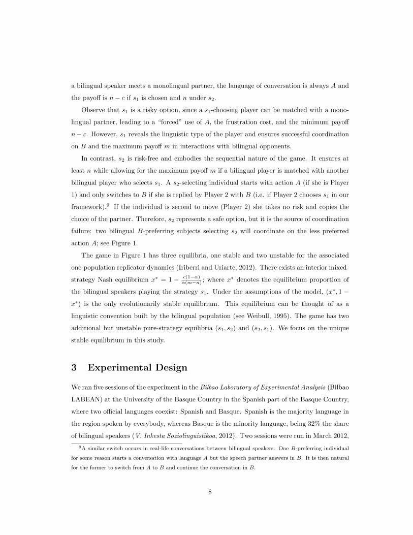
a bilingual speaker meets a monolingual partner, the language of conversation is always A and

the payoff is n− c if s1 is chosen and n under s2.

Observe that s1 is a risky option, since a s1-choosing player can be matched with a mono-

lingual partner, leading to a “forced” use of A, the frustration cost, and the minimum payoff

n− c. However, s1 reveals the linguistic type of the player and ensures successful coordination

on B and the maximum payoff m in interactions with bilingual opponents.

In contrast, s2 is risk-free and embodies the sequential nature of the game. It ensures at

least n while allowing for the maximum payoff m if a bilingual player is matched with another

bilingual player who selects s1. A s2-selecting individual starts with action A (if she is Player

1) and only switches to B if she is replied by Player 2 with B (i.e. if Player 2 chooses s1 in our

framework).9 If the individual is second to move (Player 2) she takes no risk and copies the

choice of the partner. Therefore, s2 represents a safe option, but it is the source of coordination

failure: two bilingual B-preferring subjects selecting s2 will coordinate on the less preferred

action A; see Figure 1.

The game in Figure 1 has three equilibria, one stable and two unstable for the associated

one-population replicator dynamics (Iriberri and Uriarte, 2012). There exists an interior mixed-

strategy Nash equilibrium x∗ = 1 − c(1−α)α(m−n) ; where x∗ denotes the equilibrium proportion of

the bilingual speakers playing the strategy s1. Under the assumptions of the model, (x∗, 1 −

x∗) is the only evolutionarily stable equilibrium. This equilibrium can be thought of as a

linguistic convention built by the bilingual population (see Weibull, 1995). The game has two

additional but unstable pure-strategy equilibria (s1, s2) and (s2, s1). We focus on the unique

stable equilibrium in this study.

3 Experimental Design

We ran five sessions of the experiment in the Bilbao Laboratory of Experimental Analysis (Bilbao

LABEAN) at the University of the Basque Country in the Spanish part of the Basque Country,

where two official languages coexist: Spanish and Basque. Spanish is the majority language in

the region spoken by everybody, whereas Basque is the minority language, being 32% the share

of bilingual speakers (V. Inkesta Soziolinguistikoa, 2012). Two sessions were run in March 2012,

9A similar switch occurs in real-life conversations between bilingual speakers. One B-preferring individual

for some reason starts a conversation with language A but the speech partner answers in B. It is then natural

for the former to switch from A to B and continue the conversation in B.

8

m,m;B n, n;A

m,m;B m,m;B

s2

s1

s1 s2

n;A

n− c;A

s2

s1

Nature

��

���

@@@@@R

α 1-α

Figure 1: The game played by the bilingual population. With probability α the bilingual player meets

another bilingual players and they play the game depicted in the left-hand matrix; with probability

1 − α the bilingual speaker meets a monolingual one and gets the payoffs from the right-hand table

(the monolingual speakers always receive the payoff n). Each cell in the matrix on the left contains

three letters: the payoffs of the row and column players, respectively, and the resulting language of the

conversation, A or B, in capital letters.

two in March 2013, and one in May 2014. We conducted three sessions in Spanish; two additional

sessions were run in Basque. The objective of running treatments in the two languages was to

analyze whether the linguistic conditions of subjects precondition their behavior, since bilingual

individuals find themselves frequently in real life in a situation similar to the one simulated by

our game. Hence, our study can be viewed as an artefactual experiment, i.e. conventional

experiment with a nonstandard subject pool (Harrison and List, 2004). A total of 180 students

(three sessions with 40 and two session with 30 subjects) were recruited from the undergraduate

population of the University of the Basque Country. Each session lasted approximately one

hour. The experiment was conducted using the experimental software z-Tree (Fischbacher,

2007). Subjects were given instructions explaining how they could make their choices and how

the choices would be reflected in their payoffs.10 The instructions were read aloud. Subjects

were allowed to ask any question they may have had during the whole instruction process.

Afterwards, they had to answer six control questions on the computer screen to be able to

proceed.

10The English translation of the Spanish and Basque instructions can be found in Appendix.

9

As discussed in Section 2, the experiment focuses solely on the interactions in which at least

one of the two participants is bilingual. The experiment consisted of playing 20 or 30 rounds

of the LCG depicted in Figure 1. In the first two sessions run in March 2012, subjects played

the game for 20 rounds; three 30-period sessions were run in the second and third waves of the

experiment to analyze the convergence for a longer time span.11

To be able to analyze the net effect of coordination failure, we followed the standard approach

in Economics (see Grether and Plott (1984) and Hong and Plott (1982) for early references or

Fehr and List (2004) and Palacios-Huerta and Volij (2008, 2009) for more recent examples of

artefactual experiments) and designed the experiment as neutral as possible. This is a key

aspect of our analysis because in societies where languages are in contact and typically in

conflict, bringing languages to the lab might condition participants’ behavior to a great extent.

Hence, our subjects play a sequential game with a structure similar to a conversation, in which

bilinguals may meet monolinguals. No reference to a conversation was made in the instructions

and the majority language is labelled as action A and the minority language as action B. The

only parameter found in the field and used in the experiment are the plausible proportions of

bilinguals in the population, α. We hope that this design feature allows us to separate the

coordination problems from emotional issues attached to language choice in real life.

The main interest lies in the bilingual-bilingual matches, since they allow us to evaluate the

extent of the failure to achieve the efficient outcome when two subjects loyal to language B

meet. Note that the communication involving at least one monolingual individual always forces

the use of the majority A (see Figure 1), but the possibility of monolingual-bilingual matching is

important to observe the influence of imperfect knowledge in the experiment. Since monolingual

individuals always choose the majority language A, they were simulated by computers. Hence,

all experimental subjects play the role of “bilingual” speakers in the actual experiment.12 In

each round, each subject played with another participant of the experiment with probability α,

while with probability 1− α she was matched with a computer.

We opted for the strategy method (Brandts and Charness, 2011): participants played with-

out knowing whether they move first (Player 1) or second (Player 2) and had to select the

11No time trend is observed from period 20 on in any session. Hence, we do not analyze this issue any further

below.12While describing the experimental design and results, we have to be careful distinguishing bilingual players

in the game (that is, players who can choose both action A and action B and whose role each participant of the

experiment plays) and true bilingual subjects in the experiment (i.e. the experimental subjects who speak both

Spanish and Basque). To distinguish the two terms, we label the latter as true bilinguals throughout the paper.

10

complete plan for any possible situation in the experiment. In particular, subjects were asked

to choose a plan of behavior from the following menu:

1. Plan 1 : always choose action B.

2. Plan 2 : play action A unless you know that the other player had played B. More precisely,

play A if you are the first to play and switch to B if the second player chooses B; if you

are the second player, choose the action the first player started with.

Observe that Plan 1 and Plan 2 are equivalent to strategies s1 and s2 discussed in the

previous section. Hence, Figure 1 depicts the strategic situation faced by each experimental

subject. We use the word Plan (rather than strategy) to avoid any technical terminology in the

laboratory.

All the participants face the same decision in each round and they were carefully instructed

how their choices would determine their experimental payoffs. In each period, the payoffs were

determined by the outcome of the game as follows:

• Each subject receives m = 90 experimental points (ECU) if the pair coordinates on action

B. This happens if two subjects are matched and at least one chooses Plan 1. This payoff

cannot be received in any interaction with a computer.

• Each subject receives a payoff of n = 60 ECU if the outcome of the game is (A,A). That

is, if two experimental subjects meet and both choose Plan 2, or if a participant selects

Plan 2 and is matched with a computer.

• If a subject chooses Plan 1 and is matched with a computer, she receives n−c = 60−7 = 53

ECU. By the design, this payoff can never be received in any interaction with another

participant.

The monetary payoffs were expressed in experimental currency units (ECU), converted to

Euros at the end of the experiment at the exchange rate of 100 ECU=1 Euro. Subjects earned

between 11.4 and 16.3 Euros in the twenty-period sessions and 17.1 and 24 Euros in the thirty-

period sessions. The respective averages were 13.6 and 20.1 Euros.

At the end of each round, each participant received the following feedback: her choice (Plan

1 or Plan 2), her position in the timing of the game (first or second/Player 1 or Player 2), the

11

outcome of the game ((A,A), (B,B), or (B,A))13, and her payoff.

The sessions differed in two dimensions: the probability of meeting another experimental

participant, α, and the language of the experiment (Spanish or Basque). The probability α

corresponds to the fraction of bilingual speakers in a large population of the LCG. Three sessions

were conducted in Spanish using three different values: α = 0.2, 0.4 and 0.6. Two sessions were

run in Basque for α = 0.2 and α = 0.6 (α = 0.2B and α = 0.6B, hereafter). We did not run

α = 0.4B session, because we detect little differences between the α = 0.4 and α = 0.6 sessions

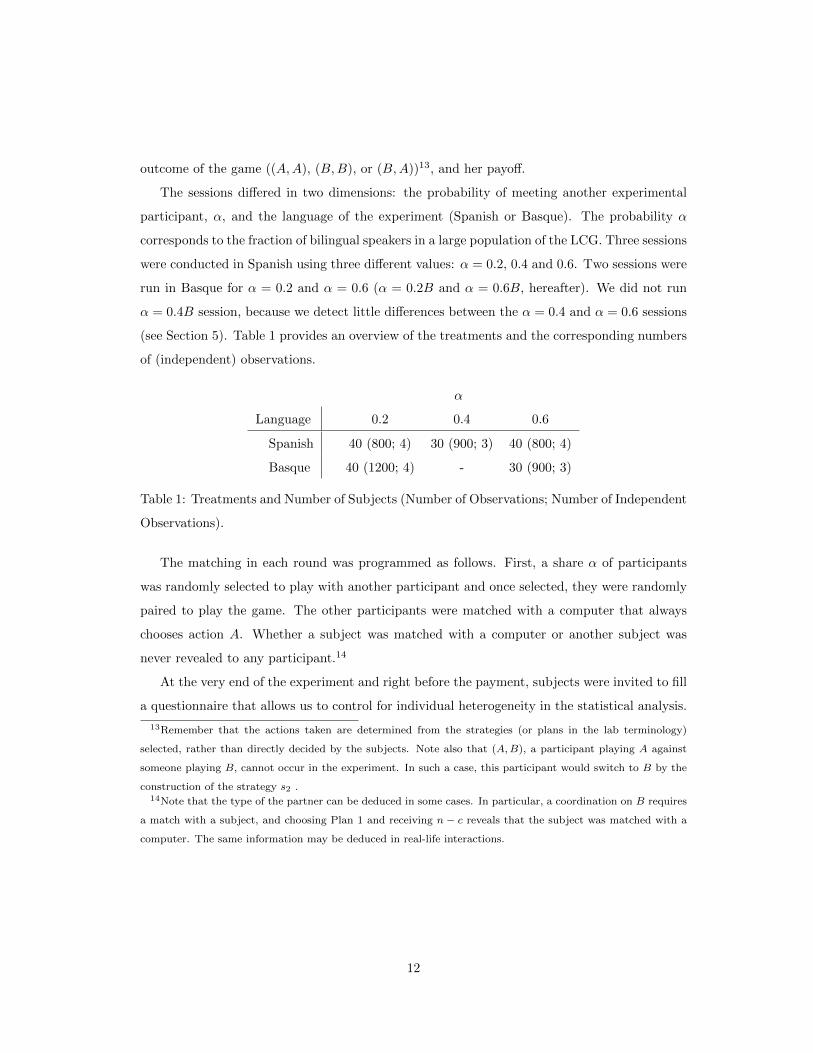
(see Section 5). Table 1 provides an overview of the treatments and the corresponding numbers

of (independent) observations.

α

Language 0.2 0.4 0.6

Spanish 40 (800; 4) 30 (900; 3) 40 (800; 4)

Basque 40 (1200; 4) - 30 (900; 3)

Table 1: Treatments and Number of Subjects (Number of Observations; Number of Independent

Observations).

The matching in each round was programmed as follows. First, a share α of participants

was randomly selected to play with another participant and once selected, they were randomly

paired to play the game. The other participants were matched with a computer that always

chooses action A. Whether a subject was matched with a computer or another subject was

never revealed to any participant.14

At the very end of the experiment and right before the payment, subjects were invited to fill

a questionnaire that allows us to control for individual heterogeneity in the statistical analysis.

13Remember that the actions taken are determined from the strategies (or plans in the lab terminology)

selected, rather than directly decided by the subjects. Note also that (A,B), a participant playing A against

someone playing B, cannot occur in the experiment. In such a case, this participant would switch to B by the

construction of the strategy s2 .14Note that the type of the partner can be deduced in some cases. In particular, a coordination on B requires

a match with a subject, and choosing Plan 1 and receiving n − c reveals that the subject was matched with a

computer. The same information may be deduced in real-life interactions.

12

4 Hypotheses

We experimentally test three main hypotheses. The first two hypotheses are based on the

unique stable equilibrium of the game in Figure 1 (see Section 2):

Hypothesis 1 (coordination failure): The rate of coordination on the efficient action B is

lower than 100% in the meetings between two participants of the experiment, irrespective of α.

Hypothesis 2 (effect of α): The higher the probability of meeting a bilingual individual

(α), the lower the extent of coordination failure in the matchings of two experimental subjects.

The third hypothesis is purely behavioral and related to the real-life monolingualism and

bilingualism of our experimental subjects. Even though all participants represent bilingual

individuals in the experiment, the truly bilingual individuals have experience with the language

choice in real-life conversations. Do their habits or conventions precondition their behavior in

the proposed neutral laboratory framework? There exist large experimental literature on the

conflict between risk and payoff dominance showing that in such situations the behavior often

converges to the risk dominant options (see Camerer (2003) and Devetag and Ortmann (2007)

for reviews). Since strategy s1 would correspond to the risky option while s2 maximizes the

minimum payoff, we hypothesize the following:

Hypothesis 3 (true bilingual subjects): Due to their real-life experience with language

choice, the true bilingual subjects choose the maximin strategy s2 more often than the true

monolingual individuals for any α.

5 Experimental Results

This section is divided into three parts. The first describes the overall results of the experiment,

the second focuses on matchings of two experimental subjects, while the last one analyzes the

effects of the real-life linguistic conditions of participants on their behavior in the two Basque

sessions.

5.1 Plan selection

Figure 2 illustrates the evolution of choices in the experiment and the effects of both treatment

variables. We plot the fraction of individual choosing the safe Plan 2 on y-axis and the ex-

perimental rounds on the x-axis. There is a monotonic association between the choice of Plan

2 and the share α. The pairwise comparisons - contrasting only treatments conducted in the

13

same language - are significantly different in the whole experiment (p < 0.001; non-parametric

Wilcoxon rank-sum tests) and from round 16 on (p < 0.003).15 In particular, on average 64%,

46.2% and 33.5% of subjects choose the safe Plan 2 for α = 0.2, 0.4 and 0.6, respectively, for

t > 15 in the Spanish sessions; the figures are 75.7 and 33.8% for α = 0.2B and 0.6B. This

ranking is corroborated in the regression analysis and robust to controlling for the effects of

experience and individual heterogeneity (see Tables 2 and 3 in Appendix). Hence, these results

confirm the Hypothesis 2: higher α induces more subjects to select the risky Plan 1 and thus

coordinate on the efficient action B.

The observed percentages are all statistically different from the shares predicted by the

mixed-strategy Nash equilibrium x∗ (p = 0 using t > 15; Wilcoxon signed-rank tests). The

predicted fractions of bilingual subjects choosing Plan 1 are 6.6%, 65%, and 84.4% for α = 0.2,

0.4, and 0.6, respectively. Hence, subjects choose Plan 1 more often than predicted in both

α = 0.2 sessions whereas less often in all α > 0.2 treatments. Section 6 provides a theoretical

justification for this regularity.

As for the language of the session, the choice of the safe Plan 2 is more frequent in the

Basque session compared to the Spanish one if α = 0.2 and t > 15 (75.7% vs. 64%; p = 0.001).

This confirms Hypothesis 3. Truly bilingual subjects more familiar with language choice in real

life tend to choose the safer option more often; this in turn results in lower coordination on

B. However, the Basque and Spanish sessions are statistically indistinguishable for α = 0.6

(p = 0.945); 33.7% and 33.5% of subjects select Plan 2, respectively. This contrasts with

Hypothesis 3.

The simplest possible test of linear time trends (random-effects logit regression of plan

selection over time and α) reveals an increasing trend of selection of Plan 2 over time in

both α = 0.2 sessions (p = 0.003 in both cases); for α > 0.2 the estimated time effects are

never significant (p > 0.27). The trends are significant in no session in the second half of the

experiment (p > 0.56), suggesting that learning takes mostly place in the initial rounds and

that the fraction of subjects playing Plan 2 converges toward a certain level, different for each α

(see Figure 2). Therefore, there seems to exist a stable language convention, in which a certain

fraction of the population ends up choosing s1 and “speaking” the minority B (as predicted

15Given the differing number of rounds in the treatments, we will only report tests based on rounds after the

fifteenth period (i.e. the last five rounds in the twenty-period sessions and the last 15 rounds in the thirty-period

sessions). All reported results are identical if we use instead (a) either the second half of the experiment in each

treatment or (b) the last five rounds in each treatment.

14

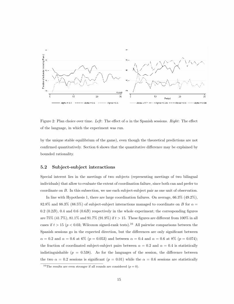
Figure 2: Plan choice over time. Left : The effect of α in the Spanish sessions. Right : The effect

of the language, in which the experiment was run.

by the unique stable equilibrium of the game), even though the theoretical predictions are not

confirmed quantitatively. Section 6 shows that the quantitative difference may be explained by

bounded rationality.

5.2 Subject-subject interactions

Special interest lies in the meetings of two subjects (representing meetings of two bilingual

individuals) that allow to evaluate the extent of coordination failure, since both can and prefer to

coordinate on B. In this subsection, we use each subject-subject pair as one unit of observation.

In line with Hypothesis 1, there are large coordination failures. On average, 66.3% (49.2%),

82.8% and 88.3% (88.5%) of subject-subject interactions managed to coordinate on B for α =

0.2 (0.2B), 0.4 and 0.6 (0.6B) respectively in the whole experiment; the corresponding figures

are 75% (41.7%), 81.1% and 91.7% (91.9%) if t > 15. These figures are different from 100% in all

cases if t > 15 (p < 0.03; Wilcoxon signed-rank tests).16 All pairwise comparisons between the

Spanish sessions go in the expected direction, but the differences are only significant between

α = 0.2 and α = 0.6 at 6% (p = 0.053) and between α = 0.4 and α = 0.6 at 8% (p = 0.074);

the fraction of coordinated subject-subject pairs between α = 0.2 and α = 0.4 is statistically

indistinguishable (p = 0.538). As for the languages of the session, the difference between

the two α = 0.2 sessions is significant (p = 0.01) while the α = 0.6 sessions are statistically

16The results are even stronger if all rounds are considered (p = 0).

15

indistinguishable (p = 0.965).17

To provide a more rigorous test, we pool the data for all treatments and control for α,

the language of the session, and the time trend using panel-data logit regressions being the

dependent variable a dummy for successful coordination on B in each subject-subject pair.

Both α (p = 0) and the language of the session (p = 0.022) affect the extent of coordination,

but there is no tendency to learn to coordinate on B over time in these encounters: period is

never significant predicting successful coordination (p = 0.77).18 Consequently, the permanent

“threat” of being matched with a computer does not allow for better coordination on the

efficient outcome over time.

These observations are also reflected in the matches of subjects with computers: subjects

matched with a computer chose the risky Plan 1 and thus miscoordinate in 40.2% (27.7%),

53.3%, and 68.4% (63.6%) of cases in the whole experiment in α = 0.2 (α = 0.2B), 0.4, and

0.6 (0.6B), respectively; the corresponding percentages are 33.1% (24.8%), 52.2%, and 65%

(63.3%) for t > 15.19

These results confirm our Hypothesis 1 that if two bilingual individuals meet they do not

necessarily coordinate on the minority B. In line with Hypothesis 2, the coordination problem

is more severe in populations with low α. Given the neutral, context-free framing of the

experiment, we posit that this may partially be attributed to coordination problems present in

language selection under imperfect information about the type of the partner.

5.3 Early vs. late bilinguals

The previous subsection provides little evidence in favor of Hypothesis 3. Being monolingual

or bilingual does not seem to influence systematically the language choice in our context-free

17The differences using all the periods are significant between α = 0.2 and both α > 0.2 sessions (p < 0.005)

and between α = 0.2 and α = 0.2B (p = 0.017). The difference between α = 0.4 and α = 0.6 is still not

significant (p = 0.105). The two α = 0.6 sessions do not differ (p = 0.948).18Similar results are obtained if we include session dummies (instead of controlling for α and the language

dummy), except that this alternative specification confirms that the language effect is driven by the α = 0.2B

session.19The pooled regression analysis shows that the frequency with which the subjects are forced to use A in the

interactions with computers increases in α and decreases over time (p = 0; pooled panel-data logit regressions).

However, the separate analysis for each treatment again detects a (decreasing) time trend only in the two α = 0.2

sessions.

16

experiment.20 To test this issue further, we ask our subjects whether their mother tongue is the

minoritarian Basque or the majoritarian Spanish. Due to the sociolinguistic conditions in the

Basque Country, this information also serves as an index of the age of acquisition of the second

language. Virtually everybody speaks Spanish in the region and all participants in the Basque

sessions were indeed bilingual. Typically, subjects reporting Basque as the mother tongue

learn Spanish simultaneously with the Basque from very early ages in everyday interactions.

In contrast, the bilingual participants naming Spanish as the mother tongue have most likely

learnt Basque at later stages at school. Following Mechelli et al. (2004), we henceforth label

the former as early bilinguals and the latter as late bilinguals.21 There are respectively 57.5%

and 46.7% of early bilinguals for α = 0.2B and α = 0.6B.

Figure 3 compares the behavior of the early and late bilinguals in both Basque sessions. We

observe that the behavior is more volatile in early rounds than in later stages, suggesting that

the behavior of both types of subjects settles over time. With the exception of rounds 9 and

10, early and late bilinguals behave similarly for α = 0.2B till period 20. However, from this

period on, the early bilingual subjects tend to select the safe Plan 2 more often. For α = 0.6B,

late bilinguals choose Plan 2 more often in the first half of the experiment, whereas the early

bilinguals choose it more often in the second half of the experiment.

Non-parametric two-sample tests confirm that the early bilingual subjects tend to choose the

safer Plan 2 more often in the last 5 (p = 0.081 and 0.033 in α = 0.2B and 0.6B, respectively)

and 10 rounds (p < 0.002). In contrast, there is no difference between the two groups in the

first 5 periods in both sessions or in the first 10 rounds for α = 0.2B (p > 0.16). In contrast, the

behavior differs statistically in the first 10 rounds for α = 0.6B but in the opposite direction:

the late bilinguals choose the safe Plan 2 more often that the early ones initially.22 Tables 4 and

5 in Appendix report regressions of the plan choice in the two Basque sessions on (i) the early-

20This does not mean that there are no behavioral consequences of the differing brain organization between

monolingual and bilingual people documented in Mechelli et al. (2004). They just do not manifest in our

context-free language-choice setup.21In the Spanish sessions, we know the mother tongue of the participants but not whether they are monolingual

or bilingual. Since only 5, 1, and 1 subjects stated Basque as the mother tongue in the α = 0.2, 0.4, and 0.6

sessions, we cannot perform any meaningful analysis of this issue in the Spanish sessions.22Comparing the early and late bilinguals with the corresponding Spanish sessions uncovers no differences

across the people according to their language conditions in the first five rounds (p > 0.14), except a marginal

difference between the late bilinguals and Spanish-session participants for α = 0.2 (p = 0.093). Hence, the

linguistic condition of participants does not seem to influence the initial play. Most of the differences become

significant over time as subjects learn.

17

Figure 3: The choices in the Basque sessions, disaggregated for the early and late bilinguals.

bilingual dummy, (ii) period, and (iii) the interaction between period and the early-bilingual

dummy, disaggregated for α = 0.2B and α = 0.6B. It shows that the differences observed at

the end of the experiment come from the evolution of the behavior: the early-bilinguals dummy

is rarely significant whereas the interactions between this dummy and period is significant,

independently of the specification of the models. The early bilinguals are e0.04 = 1.038 and

1.073 times more likely to choose the safe option with each additional period in the α = 0.2B

and 0.6B, respectively. Hence, the two groups are not different initially but the early bilingual

subjects tend to increase the use of the safe Plan 2 over time while the late bilinguals decrease

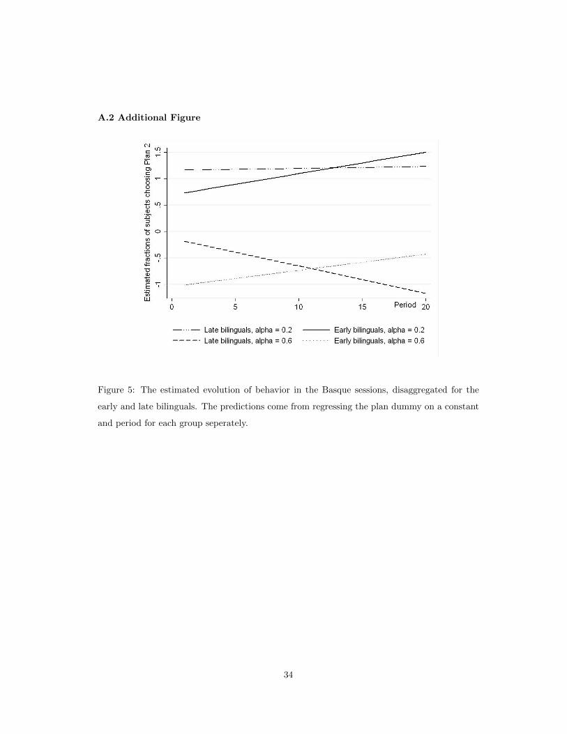
it.23 Figure 5 in Appendix provides a visualization of the predicted tendencies.

6 Non-equilibrium behavior

The experimental results exhibit two regularities that cannot be explained by the equilibrium

analysis of the game in Figure 1: (a) the experimental subjects play the safe Plan 2 more

often than predicted by the equilibrium if α = 0.2 and less often if α > 0.2, and (b) the early

23The results are identical if we pool both Basque sessions into one regression.

18

bilingual individuals learn to choose the safe Plan 2 more often than both the monolingual

and late bilingual subjects. Can we find theoretical arguments that would justify these two

phenomena?

To answer this question, let us hereafter assume that people are boundedly rational and

disappointment averse. To model the former, we apply the logistic specification of McKelvey

and Palfrey’s (1999) quantal response equilibrium (QRE). Rather than assuming that people

play their response with probability one, this approach posits that their behavior is noisy.24

More precisely, each pure strategy is selected with some positive probability that increases with

the expected payoff of the strategy. Hence, more costly mistakes are less likely. The degree of

bounded rationality is reflected by a parameter λ ≥ 0. If λ = 0, people choose randomly; as

λ → ∞ people become more rational and QRE converges to a Nash prediction. In our game,

the QRE converges to the unique stable equilibrium from Section 2.

Additionally, we assume that individuals are averse to disappointment a la Gul (1991). Gul’s

approach can be understood as one of the reference-dependent models of preferences, in which

people compare their payoffs with the certainty equivalents. If the realized payoffs are lower

than the certainty equivalent, people suffer disutility proportional to their degree of aversion

to disappointment, denoted as β, and the difference between the utility from the outcome and

the utility from the certainty equivalent. Formally,

U(x) = E[x]− βE[µ− x|µ > x],

where µ is the certain amount that gives the player the same utility as the (uncertain) option

x.

Recall that in the unique stable Nash equilibrium each player plays the strategy s1 with

probability x∗ = max{0, 1 − c(1−α)α(m−n)}. Under limited rationality, the analogous symmetric

equilibrium, in which we assume a common parameter of disappointment aversion, is xD =

max{0, 1− c(1−α)(1+β)α(m−n) } ≤ x

∗. The following result establishes the relation among the equilibria

under the different utility specifications:25

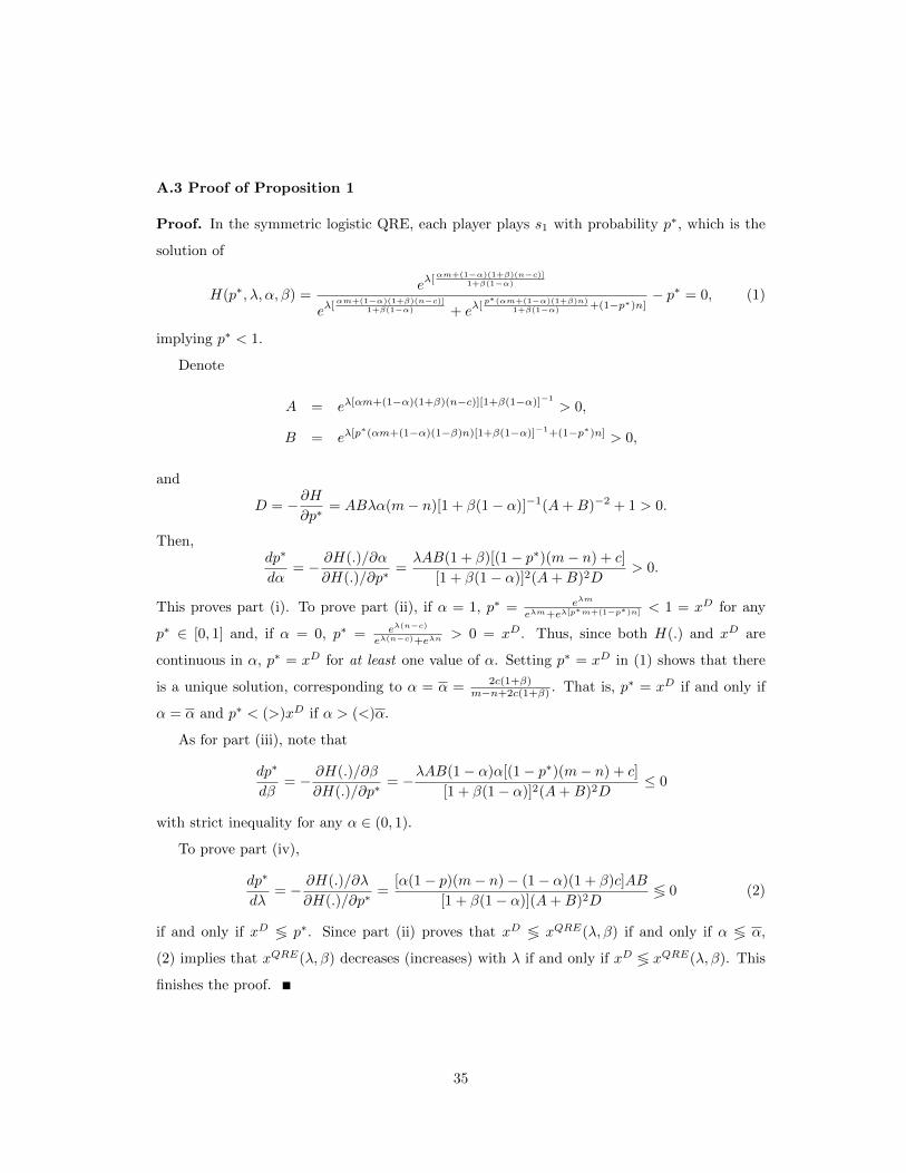
Proposition 1 Assume that each player is averse to disappointment with a parameter β ≥ 0

and c < (m − n) α1−α . Then, in the symmetric logistic Quantal Response Equilibrium of the

game in Figure 1, the probability xQRE(λ, β) of playing strategy s1 satisfies the following:

24The noise can represent simple mistakes, limited reasoning abilities of players etc.25See Appendix for the proof.

19

(i) xQRE(λ, β) < 1 and xQRE(λ, β) increases in α for any λ > 0 and β ≥ 0.

(ii) There exists a threshold α such that xQRE(λ, β) ≥ xD for α ≤ α and xQRE(λ, β) ≤ xD

for α ≥ α (with strict inequalities when α ≶ α).

(iii) xQRE(λ, β) (weakly) decreases in β for any λ > 0.

(iv) For λ′ > λ, xD ≤ xQRE(λ′, β) < xQRE(λ, β) if α ≤ α, while xD ≥ xQRE(λ′, β) >

xQRE(λ, β) if α ≥ α.

Each part of Proposition 1 provides one insight. Part (i) shows that Hypotheses 1 and 2 still

hold in this setup: coordination failure should exist for any α and lower α’s should aggravate

the coordination problems in equilibrium.

The second part shows that the non-equilibrium regularity (a) can be attributed to bounded

rationality: relaxing perfect rationality drives the coordination rates up or down if α lies,

respectively, below or above a certain threshold α. If the aversion to disappointment is not too

large, this threshold lies between α = 0.2 and α = 0.4, matching the behavior observed in the

lab. In particular, for our experimental parameters α = 0.32 if β = 0 and α < 0.4 if β < 0.428.

Part (iii) illustrates the effect of disappointment aversion and relates to why some people

may systematically choose s1 more or less often than others. Particularly, disappointment

aversion pushes the number of s1-choosing individuals down in the equilibrium (be it the fully

rational Nash or the boundedly rational QRE). The intuition behind this result is that more

disappointment-averse individuals give more weight (with respect to standard utility specifica-

tions) to payoff realizations below the certainty equivalent, lowering thus the expected utilities

of options that may lead to payoffs below this threshold. Consequently, any model attaching

such extra weights to lower payoffs would generate the same effect as disappointment aver-

sion. Examples of such models include risk aversion,26 regret aversion a la Loomes and Sugden

(1982), or the loss aversion with respect to certain reference point (e.g. rank-dependent model

of Koszegi and Rabin, 2006). We selected the linear specification of Gul’s (1992) model for the

sake of simplicity but any of these alternative models would work too. Hence, Proposition 1

predicts the early bilingual individuals to play the risky Plan 1 less often than the late bilinguals

for any α if the former are more averse to disappointment, risk, regret, and/or losses. Is this

what we observe in the data?

26In fact, Gul (1992) shows that there is a strong link between risk aversion and his disappointment aversion.

20

We find little support for any of these models in the data.27 Tables 4 and 5 in Appendix

show that the early and late bilinguals exhibit no different reactions to the between-round

experience.28 That is, neither the early nor late bilinguals react differently to disappointing

outcomes or outcomes below the rational expectations (e.g. choosing the risky Plan 1 and being

miscoordinated), providing indirect evidence against the disappointment or regret aversion, or

loss aversion a la Koszegi and Rabin (2006). Moreover, the difference is unlikely to be due to

different reference points, because both types are identical in the early stages of the experiment

and only different reactions to the experience would suggest different evolution of the reference

points over time. However, we cannot observe the reference points people hold. We also find

little support for differing risk aversion between the two types. The early bilinguals are indeed

more risk averse in three non-incentivized risk-related questions in the questionnaire but the

differences are statistically weak (both testing the differences questions by question, p > 0.19,

or using the combination of all the variables, p = 0.304). Controlling systematically for these

variables in the regression analysis does relate with the behavior in the experiment in the

expected direction, but affects neither the early bilingual dummy nor the interaction between

this dummy and period.29

Last, Part (iv) of Proposition 1 rules out two candidate explanations of the documented

differences between the early and late bilinguals. First, due to their special linguistic conditions

early bilinguals might posses specific cognitive abilities and thus be less or more boundedly

rational (systematically higher or lower λ’s). Alternatively, one may argue that the early

bilinguals may have relatively more experience with a situation simulated in our experiment,

suggesting more rational behavior and less mistakes (higher λ’s).30 If one of these arguments

lies behind the difference between the two types, then Proposition 1 predicts one type to play

the safe Plan 2 more often than the other type above a certain value of α and the contrary

below that value. In contrast, the early bilinguals learn to play the safe option systematically

more often independently of α.

27Since estimating the model parameters for the individual model, jointly with QRE parameter λ, would

require additional assumptions, we do not estimate them here and only rely on the indirect evidence.28We also ran regressions including, in addition to the variables used in Tables 4 and 5, the interaction

between the early bilingual dummy and the different experience-related variables. These regressions confirm

that there are no systematic difference of how each type of bilingual individuals reacts to past experience and

the interactions between period and the early bilingual dummy remains significant at these models. We do not

report these estimations.29To save on space we do not report the details of these estimations here.30McKelvey and Palfrey (1995) report that experience increases the estimated λ’s in the experiments.

21

In sum, bounded rationality explains why the subjects systematically choose certain options

less or more often than predicted and rules out the cognitive- and experience-based explanations

of the detected differences between the early and late bilinguals. Indeed, cognitive reflection

test and IQ-related questions are unrelated to subjects’ play in the regressions and they are no

different in these terms. The considered behavioral approaches and risk aversion can tell why

some people behave differently than others but we find little support for these theories in the

data.

7 Conclusions

This study analyzes whether the failure to speak minority languages may be partially attributed

to incomplete information about the linguistic type of speech partners and coordination fail-

ure, two phenomena widely studied in economics. To this aim, we simulate experimentally

a strategic situation resembling language choice in real-life anonymous interactions, using a

context-free framing to be able to isolate the effect of the coordination failure from emotions

commonly attached to linguistic issues. We report that the miscoordination on minority lan-

guages between people that “speak” the language is persistent and more likely if the language

is more minoritarian, more endangered. Moreover, the ability to coordinate on the preferred

option in our context-free experiment correlates with real-life linguistic conditions of subjects.

Early bilingual subjects (people whose mother tongue is the minoritarian Basque) learn to play

the safe, minority language-harming strategies more than other subjects.

Which part of the difference between the knowledge and use of minority languages can be

attributed to imperfect information in real life? Figure 4 contrasts our experimental results

with real-life language knowledge and use in the in the Spanish part of the Basque Country.31

The minority-language knowledge, corresponding to α, is measured on the x-axis and its use

on the y-axis. The empty circles (full circles/triangles) represent the field (experimental) data.

Each dot represents one municipality (treatment) and the y-value is the proportion of the sam-

pled inhabitants of the municipality who took part in a conversation in the minority Basque

31This region satisfies the conditions simulated by our experimental design: (i) it belongs to an economically

advanced country with high mobility of the population, leading to frequent meetings of unrelated individuals,

(ii) it faces a linguistic conflict between two linguistically distant languages, the majoritarian Spanish spoken

by everybody and the minoritarian Basque spoken by 32% of the population, and (iii) the survival of the

minoritarian language and its co-officiality reflects the loyalty to it.

22

language (the percentage of the experimental population achieving to coordinate on action B

for t > 15).32 The data would lie on the (dashed) 45o line if all the bilingual individuals in each

Basque municipality used the minority Basque in every conversation, something impossible if

they interact with non-bilingual individuals. Figure 3 illustrates the discrepancies between the

minority-language use and knowledge in real-life, how it varies non-linearly with α, and how

the experimental observations match these facts. The figure suggests that the coordination

failure may account for a relevant part of the discrepancy. However, due to differing data-

collection techniques, we cannot perform rigorous comparison of the field and the experimental

observations and thus evaluate quantitatively the relative impact of imperfect-information is-

sues.33 Most importantly, the real-life meetings are assortative and often far from anonymous

(e.g. McPherson et al., 2007), we suspect that Figure 4 exaggerates the relative importance of

incomplete information in language choice.

Our findings show that game-theoretical analysis of language choice can inform policies

targeting the minority language survival in multilingual societies. Minority languages and their

related cultures are in danger of being shifted by the majority language (Fishman, 1991) and

the economic literature increasingly recognizes the benefits of linguistic diversity (Ginsburgh

and Weber, 2011; Grin et al., 2010). To cope with the enormous power and social presence

of the majoritarian languages, only active linguistic policies coupled with bilingual speakers’

language behavior may avoid the shifting process of the minority language. This is all the more

so when A and B are linguistically distant, since the costs of a language policy to promote B are

higher in these cases. There are few particular policy messages. Apart from common policies

targeting α through education, the authorities should actively promote the status of minority

languages and provide coordination devices that lower the imperfect information.34 In terms

32For example, 75% of subject-subject pairs coordinating on B for α = 0.2 and t > 15 represents a society,

in which 3% (0.75× 0.22) use the minority language in their conversations if we assume random matching. The

percentages are 12.98% and 33.01% for α = 0.4 and 0.6, and 1.67% and 33.08% for α = 0.2B and 0.6B.33The experimental data and the theory are based on pairwise random anonymous interactions and any

emotional feelings toward any of the “languages” has been removed. In contrast, the field data are based on

language use in randomly chosen conversations on the street, without manipulating the number of participants in

each conversation nor who meets with whom. Since all these aspects violate our assumptions, the experimental

data may both over- and underestimate the pure effect of coordination failure. The available data do not allow

to treat these differences econometrically.34Examples of such devices is the obligation of public employees who interact with the general population to

speak the minority languages, documenting and publicizing places, where one can be attended in her language

etc.

23

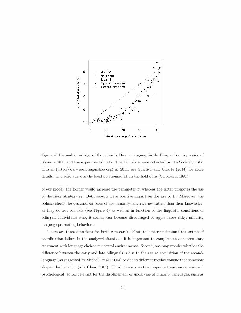
Figure 4: Use and knowledge of the minority Basque language in the Basque Country region of

Spain in 2011 and the experimental data. The field data were collected by the Sociolinguistic

Cluster (http://www.soziolinguistika.org) in 2011; see Sperlich and Uriarte (2014) for more

details. The solid curve is the local polynomial fit on the field data (Cleveland, 1981).

of our model, the former would increase the parameter m whereas the latter promotes the use

of the risky strategy s1. Both aspects have positive impact on the use of B. Moreover, the

policies should be designed on basis of the minority-language use rather than their knowledge,

as they do not coincide (see Figure 4) as well as in function of the linguistic conditions of

bilingual individuals who, it seems, can become discouraged to apply more risky, minority

language-promoting behaviors.

There are three directions for further research. First, to better understand the extent of

coordination failure in the analyzed situations it is important to complement our laboratory

treatment with language choices in natural environments. Second, one may wonder whether the

difference between the early and late bilinguals is due to the age at acquisition of the second-

language (as suggested by Mechelli et al., 2004) or due to different mother tongue that somehow

shapes the behavior (a la Chen, 2013). Third, there are other important socio-economic and

psychological factors relevant for the displacement or under-use of minority languages, such as

24

the role of signals, face-to-face interactions, and social networks. We will target these issues in

future research.

References

[1] Abrams, D. M., & Strogatz, S. H. (2003). Linguistics: Modelling the dynamics of language

death. Nature, 424(6951), 900-900.

[2] Blume, A. (2000). Coordination and learning with a partial language. Journal of Economic

Theory, 95(1), 1-36.

[3] Blume, A. and O. Board (2013). Language barriers. Econometrica 81(2), 781-812.

[4] Brandts, J., & Charness, G. (2011). The strategy versus the direct-response method: a

first survey of experimental comparisons. Experimental Economics, 14(3), 375-398.

[5] Camerer, C. (2003). Behavioral game theory: Experiments in strategic interaction. Prince-

ton University Press.

[6] Caminal, R. (2010) “Markets and Linguistic Diversity,” Journal of Economic Behavior and

Organization, 76, 774-790.

[7] Chen, M. K. (2013). The effect of language on economic behavior: Evidence from savings

rates, health behaviors, and retirement assets. American Economic Review, 103(2), 690-

731.

[8] Cleveland, W.S. (1981) LOWESS: A program for smoothing scatterplots by robust locally

weighted regression, The American Statistician 35, 54.

[9] Cooper, D. J., Kagel, J. H., Lo, W., & Gu, Q. L. (1999). Gaming against managers in

incentive systems: Experimental results with Chinese students and Chinese managers.

American Economic Review 89, 781-804.

[10] Crystal D. (2001) Language Death. Cambridge: Cambridge University Press.

[11] Crystal D (1987) The Cambridge Encyclopedia of Language. Cambridge: Cambridge Uni-

versity Press.

25

[12] Devetag, G., & Ortmann, A. (2007). When and why? A critical survey on coordination

failure in the laboratory. Experimental Economics, 10(3), 331-344.

[13] Fehr, E., & List, J. A. (2004). The hidden costs and returns of incentives—trust and

trustworthiness among CEOs. Journal of the European Economic Association 2, 743-771.

[14] Ferrer i Cancho R, Sole R.V. (2003) Least effort and the origins of scaling in human

language. Proceedigs of the National Academy of Sciences 100: 788–791.

[15] Fischbacher, U. (2007), ”z-Tree: Zurich toolbox for ready-made economic experiments,”

Experimental Economics 10, 171–178.

[16] Fishman JA (1991) Reversing Language Shift: Theoretical and Empirical Foundations of

Assistance to Threatened Languages. Clevedon: Multilingual Matters.

[17] Fishman JA (2001) Why is it so hard to save a threatened language? In: Fishman JA

(ed.) Can Threatened Languages Be Saved? Clevedon: Multilingual Matters: pp. 1–23.

[18] Ginsburgh, V. and Weber, S. (2011) How Many Languages Do We Need? The Economics

of Linguistic Diversity. Princeton, NJ: Princeton University Press.

[19] Grin, F., Sfreddo, C. and Vaillancourt, F. (2010) The Economics of the Multilingual Work-

place. New York, NY: Routledge.

[20] Grether, D. M., & Plott, C. R. (1984). The Effects of Market Practices in Oligopolistic

Markets: An Experimental Examination of the Ethyl Case. Economic Inquiry 22, 479–507.

[21] Gul, F. (1991), ”A theory of disappointment aversion,” Econometrica 59, 667-686.

[22] Harrison, G.W., & List, J. A. (2004), “Field Experiments,” Journal of Economic Literature

42, 1009–1055.

[23] Harsanyi, J. C., & Selten, R. (1988). A general theory of equilibrium selection in games

(Vol. 1). The MIT Press.

[24] Hong, J. T. & Plott, C. R. (1982). Rate Filing Policies for Inland Water Transportation:

An Experimental Approach, Bell Journal of Economics 13, 1–19.

[25] Iriberri, N. and Uriarte, J.R. (2012), ”Minority language and the stability of bilingual

equilibria”. Rationality and Society, 24(4): 442-462.

26

[26] Koszegi, B., & Rabin, M. (2006). A model of reference-dependent preferences. The Quar-

terly Journal of Economics 121, 1133-1165.

[27] Loomes, G., & Sugden, R. (1982). Regret theory: An alternative theory of rational choice

under uncertainty. The Economic Journal 92, 805-824.

[28] McKelvey, R. D., & Palfrey, T. R. (1995). Quantal response equilibria for normal form

games. Games and Economic Behavior 10, 6-38.

[29] McPherson, M., Smith-Lovin, L., & Cook, J. M. (2001). Birds of a feather: Homophily in

social networks. Annual Review of Sociology 27, 415-444.

[30] Mechelli, A., Crinion, J. T., Noppeney, U., O’Doherty, J., Ashburner, J., Frackowiak, R.

S., & Price, C. J. (2004): Neurolinguistics: structural plasticity in the bilingual brain,

Nature 431, 757-757.

[31] Palacios-Huerta, I. & Volij, O. (2008). Experientia docet: Professionals play minimax in

laboratory experiments. Econometrica 76, 71–115.

[32] Palacios-Huerta, I., & Volij, O. (2009). Field centipedes. American Economic Review 99,

1619-1635.

[33] Patriarca, M., Castello, X., Uriarte, J. R., Eguıluz, V. M., & San Miguel, M. (2012).

Modeling two-language competition dynamics. Advances in Complex Systems 15(03n04).

[34] Rubinstein, A. (2000) Economics and Language, Cambridge: CUP.

[35] Selten, R., & Warglien, M. (2007). The emergence of simple languages in an experimental

coordination game. Proceedings of the National Academy of Sciences, 104(18), 7361-7366.

[36] Sperlich, S. & Uriarte, J.R. (2014). The Economics of ”Why is it so hard to save a threat-

ened Language?” Ikerlanak Working Paper 2014-77.

[37] V. Inkesta Soziolinguistikoa. Euskal Autonomia Erkidegoa. Basque Government. 2012.

[38] Van Huyck, J. B., Battalio, R. C., & Beil, R. O. (1990). Tacit coordination games, strategic

uncertainty, and coordination failure. American Economic Review, 80(1), 234-248.

[39] Van Huyck, J. B., Battalio, R. C., & Beil, R. O. (1991). Strategic uncertainty, equilib-

rium selection, and coordination failure in average opinion games. Quarterly Journal of

Economics, 106(3), 885-910.

27

[40] Weber, R. A., & Camerer, C. F. (2003). Cultural conflict and merger failure: An experi-

mental approach. Management Science, 49(4), 400-415.

[41] Weibull, J.W. (1995) Evolutionary Game Theory. Cambridge, MA: The MIT Press.

[42] Wickstrom, B.-A. (2005) Can bilingualism be dynamically stable? Rationality and Society

17: 81–115.

[43] Winford, D. (2003) An Introduction to Contact Linguistics. Oxford, UK: Blackwell.

28

Appendix

A Additional results

A.1 Regression analysis

The experimental data constitute a panel, being subjects the cross-sectional variable and rounds

the time series. The dependent variable is binary, taking values of zero (one) if a subject in a

particular round choose Plan 1 (Plan 2). We estimate random-effect logistic regression models.

Four model specifications are used:

1. Treatment effects (estimations (1) in Tables 2 and 3): effects of α, a dummy for the

Basque session, and controlling for any remaining trends in the data over time (variable

period).

2. Treatment effects and history (estimations (2) in Tables 2 and 3): These models add four

variables controlling for individual experience to the specification (1). In particular, we

control for whether the last round was miscoordinated or not (Miscoor. in the tables),

whether coordination occurred after a choice of Plan 1 (Coord. B & Plan 1 ), whether

coordination occurred after a choice of Plan 2 (Coord. B & Plan 2 ), and whether the

subjects played first (First) in the previous round. Hence, the reference category is having

chosen the risky Plan 1 and being coordinated.

3. Treatment effects, history, and individual (time-invariant) heterogeneity (estimations (3)

in Tables 2 and 3): These models, apart from the above, control for heterogeneity from

the questionnaires (such as gender, native language, risk aversion, cognitive reflection,

social values etc.).

4. Subjects who state the minoritarian Basque language as the mother tongue (early bilin-

guals) vs. the remaining participants (late bilinguals) in the Basque sessions (Table 4 for

α = 0.2B; Table 5 for α = 0.6B): These models explore the differences between the two

types of individuals, focusing on the dynamics of their choices and the way they react

to previous experience. The different models are structured the same way as the above

specifications.

29

(1) (2) (3)

Period .01∗∗∗ .008 .008

(.005) (.005) (.005)

Alpha -4.51∗∗∗ -4.32∗∗∗ -4.25∗∗∗

(.70) (.62) (.63)

Basque session 0.57∗∗ .53∗∗ .71∗∗∗

(.26) (.23) (.26)

Miscoor. - -.77∗∗∗ -.75∗∗∗

(.10) (.10)

Coord. B & Plan 1 - -.38∗∗∗ -.33∗∗∗

(.11) (.12)

Coord. B & Plan 2 - .90∗∗∗ .92∗∗∗

(.15) (.15)

First - .05 .03

(.08) (.08)

Cons. 1.33∗∗∗ 1.55∗∗∗ 2.01∗∗∗

(.33) (.29) (.57)

Heterogeneity No No Yes

Obs. 4600 4420 4276

p (model) 0 0 0

LL -2478 -2314 -2230

Table 2: Random-effects logistic regression: Probability of selecting Plan 2 (using α and a

dummy for the Basque sessions). Note: *** - significant at 1%, ** - 5%, * - 10%; Micoord.,

Coord. B & Plan 1, and Coord. B & Plan 2, and First are laggs from the previous round. The

first three denote miscoordination, coordination on B while choosing Plan 1, and coordinating

on B while choosing Plan 2; the refence catogory is having chosen Plan 2 and being coordinated

on A. The same applies to Tables 3-5.

30

(1) (2) (3)

Period .01∗∗∗ .008∗ .008∗

(.005) (.005) (.005)

α = 0.2B .79∗∗ .74∗∗ .81∗∗

(0.38) (.33) (.36)

α = 0.4 -.94∗∗ -.90∗∗ -1.04∗∗∗

(.41) (.36) (.37)

α = 0.6 -1.52∗∗∗ -1.45∗∗∗ -1.50∗∗∗

(.39) (.34) (.36)

α = 0.6B -1.32∗∗∗ -1.28∗∗∗ -1.05∗∗∗

(.41) (.35) (.38)

Miscoor. - -.77∗∗∗ -.75∗∗∗

(.10) (.10)

Coord. B & Plan 1 - -.38∗∗∗ -.33∗∗∗

(.11) (.12)

Coord. B & Plan 2 - .90∗∗∗ .92∗∗∗

(.15) (.15)

First - .05 .03

(.08) (.08)

Cons. .33 -.59∗∗ 1.20∗∗

(.27) (.24) (.53)

Heterogeneity No No Yes

Obs. 4600 4420 4276

p (model) 0 0 0

LL -2477 -2313 -2230

Table 3: Random-effects logistic regression: Probability of selecting Plan 2 (using session dum-

mies, being α = 0.2 the reference group). Note: *** - significant at 1%, ** - 5%, * - 10%.

31

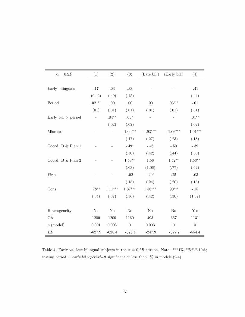
α = 0.2B (1) (2) (3) (Late bil.) (Early bil.) (4)

Early bilinguals .17 -.39 .33 - - -.41

(0.42) (.49) (.45) (.44)

Period .02∗∗∗ .00 .00 .00 .03∗∗∗ -.01

(01) (.01) (.01) (.01) (.01) (.01)

Early bil. × period - .04∗∗ .03∗ - - .04∗∗

(.02) (.02) (.02)

Miscoor. - - -1.00∗∗∗ -.93∗∗∗ -1.06∗∗∗ -1.01∗∗∗

(.17) (.27) (.23) (.18)

Coord. B & Plan 1 - - -.49∗ -.46 -.50 -.39

(.30) (.42) (.44) (.30)

Coord. B & Plan 2 - - 1.53∗∗ 1.56 1.52∗∗ 1.53∗∗

(.63) (1.06) (.77) (.62)

First - - -.02 -.40∗ .25 -.03

(.15) (.24) (.20) (.15)

Cons. .78∗∗ 1.11∗∗∗ 1.37∗∗∗ 1.58∗∗∗ .90∗∗∗ -.15

(.34) (.37) (.36) (.42) (.30) (1.32)

Heterogeneity No No No No No Yes

Obs. 1200 1200 1160 493 667 1131

p (model) 0.001 0.003 0 0.003 0 0

LL -627.9 -625.4 -578.4 -247.9 -327.7 -554.4

Table 4: Early vs. late bilingual subjects in the α = 0.2B session. Note: ***1%,**5%,*-10%;

testing period + early.bil.×period=0 significant at less than 1% in models (2-4).

32

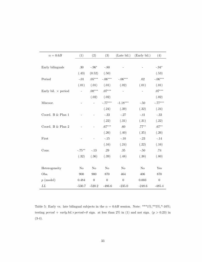
α = 0.6B (1) (2) (3) (Late bil.) (Early bil.) (4)

Early bilinguals .30 -.96∗ -.80 - - -.94∗

(.43) (0.52) (.50) (.53)

Period -.01 .05∗∗∗ -.06∗∗∗ -.06∗∗∗ .02 -.06∗∗∗

(.01) (.01) (.01) (.02) (.01) (.01)

Early bil. × period - .08∗∗∗ .07∗∗∗ - - .07∗∗∗

(.02) (.02) (.02)

Miscoor. - - -.77∗∗∗ -1.18∗∗∗ -.50 -.77∗∗∗

(.24) (.39) (.32) (.24)

Coord. B & Plan 1 - - -.33 -.27 -.41 -.33

(.22) (.31) (.31) (.22)

Coord. B & Plan 2 - - .67∗∗∗ .60 .77∗∗ .67∗∗

(.26) (.40) (.35) (.26)

First - - -.15 -.10 -.23 -.14

(.16) (.24) (.22) (.16)

Cons. -.75∗∗ -.13 .29 .35 -.50 .74

(.32) (.36) (.39) (.48) (.38) (.80)

Heterogeneity No No No No No Yes

Obs. 900 900 870 464 406 870

p (model) 0.484 0 0 0 0.003 0

LL -530.7 -520.2 -486.6 -235.0 -248.6 -485.4

Table 5: Early vs. late bilingual subjects in the α = 0.6B session. Note: ***1%,**5%,*-10%;

testing period + early.bil.×period=0 sign. at less than 2% in (1) and not sign. (p > 0.23) in

(3-4).

33

A.2 Additional Figure

Figure 5: The estimated evolution of behavior in the Basque sessions, disaggregated for the

early and late bilinguals. The predictions come from regressing the plan dummy on a constant

and period for each group seperately.

34

A.3 Proof of Proposition 1

Proof. In the symmetric logistic QRE, each player plays s1 with probability p∗, which is the

solution of

H(p∗, λ, α, β) =eλ[

αm+(1−α)(1+β)(n−c)]1+β(1−α)

eλ[αm+(1−α)(1+β)(n−c)]

1+β(1−α) + eλ[p∗(αm+(1−α)(1+β)n)

1+β(1−α)+(1−p∗)n]

− p∗ = 0, (1)

implying p∗ < 1.

Denote

A = eλ[αm+(1−α)(1+β)(n−c)][1+β(1−α)]−1

> 0,

B = eλ[p∗(αm+(1−α)(1−β)n)[1+β(1−α)]−1+(1−p∗)n] > 0,

and

D = −∂H∂p∗

= ABλα(m− n)[1 + β(1− α)]−1(A+B)−2 + 1 > 0.

Then,dp∗

dα= − ∂H(.)/∂α

∂H(.)/∂p∗=λAB(1 + β)[(1− p∗)(m− n) + c]

[1 + β(1− α)]2(A+B)2D> 0.

This proves part (i). To prove part (ii), if α = 1, p∗ = eλm

eλm+eλ[p∗m+(1−p∗)n] < 1 = xD for any

p∗ ∈ [0, 1] and, if α = 0, p∗ = eλ(n−c)

eλ(n−c)+eλn> 0 = xD. Thus, since both H(.) and xD are

continuous in α, p∗ = xD for at least one value of α. Setting p∗ = xD in (1) shows that there

is a unique solution, corresponding to α = α = 2c(1+β)m−n+2c(1+β) . That is, p∗ = xD if and only if

α = α and p∗ < (>)xD if α > (<)α.

As for part (iii), note that

dp∗

dβ= − ∂H(.)/∂β

∂H(.)/∂p∗= −λAB(1− α)α[(1− p∗)(m− n) + c]

[1 + β(1− α)]2(A+B)2D≤ 0

with strict inequality for any α ∈ (0, 1).

To prove part (iv),

dp∗

dλ= − ∂H(.)/∂λ

∂H(.)/∂p∗=

[α(1− p)(m− n)− (1− α)(1 + β)c]AB

[1 + β(1− α)](A+B)2D≶ 0 (2)

if and only if xD ≶ p∗. Since part (ii) proves that xD ≶ xQRE(λ, β) if and only if α ≶ α,

(2) implies that xQRE(λ, β) decreases (increases) with λ if and only if xD ≶ xQRE(λ, β). This

finishes the proof.

35

B Instructions

WELCOME TO THE EXPERIMENT!

This experiment analyzes how people make their choices.

We do not expect from you any particular behavior. Just bear in mind that your choices

will affect the amount of money you will earn. However, independently of your behavior you

can never loose money.

In the following, you will find instructions of how the experiment works and how you can

use the computer during the experiment.

Please, do not talk to other participants of the experiment. If you need any help, raise your

hand and one of the experimenter will attend you as soon as possible.

We would also like to ask you to turn off you cell phones and not to use them during the

experiment.

THE EXPERIMENT

• The experiment consists of 20 rounds.

• In each of these rounds, you will participate in the game that we explain below.

• In each round, you will be randomly paired either with a computer or with another

participant of this experiment.

• You will never know whether you were paired with a computer or a person, neither who

that person is in the latter case.

• The amount you earn depends on how you play, with whom you play, and how the other

player plays.

• During the experiment, we will use points as a measure of payment, but at the end of the

experiment you will be paid the full amount in euros at the exchange of 1 per 100 points

(100 points = 1 e).

THE GAME

• In each of the 20 rounds, you will play the same game.

36

• There are two players in the game. You are one of them. The other player is a computer

or a person in this room chosen at random.

• At the end of each round, you will be paired with a new player (computer or participant).

• There are two possible actions in the game: A or B.

• With 60% probability you will be paired with a computer. The computer always plays

A.35

• With 40% probability you will be matched with someone else from this room and she,

like you, can do A or B.

• The game is sequential. The sequence of the game is as follows: one player chooses first;

then it is the turn of the second player, after which the former has the option to change

her choice.

• The outcome of the game is determined by the final actions of both players.

• In each round, you will play without knowing if you are first or the second. You will not

know your position! With probability 0.5 you will choose first and with probability 0.5

you will choose second.

YOUR PARTICIPATION

In each round, your participation consists of choosing in a plan of behavior from 2 options:

1. Plan 1: always choose action B.

2. Plan 2: play action A unless you know that the other player had played B. More

precisely, play A if you are the first to play and switch to B if the second player chooses

B; if you are the second player, choose the action the first player started with.

Note that under Plan 1 you choose B regardless of the position you occupy in the game and

the other player’s choice. However, under Plan 2 you choose A or B depending on the position

you occupy in the game and the other player’s choice.

35Remember that one of the treatment variables is the share of bilingual speakers, α. Hence, the only difference

across the treatments concerning the instructions comes from the differing shares. These instructions are from

α = 0.4.

37

THE OUTCOME OF THE GAME AND THE PAYOFFS

• If the other player is a computer and you choose Plan 1, the outcome of the game will be

A for the computer and B for you. As a result, your payment will be equal to 53 points.

• If the other player is a computer and you choose Plan 2, the outcome of the game will be

A for both and your payment will be equal to 60 points.

• If the other player is another person in the room and both of you choose Plan 1, the

outcome of the game will be B for both and your payment will be equal to 90 points.

• If the other player is another person in the room who chooses Plan 1 and you choose Plan

2, the outcome of the game will be B for both. So, your payment will be equal to 90

points.

• If the other player is another person in the room who chooses Plan 2 and you choose Plan

1, the outcome of the game will be B for both. So, your payment will be equal to 90

points.

• If the other player is another person in the room and both of you choose Plan 2, the

outcome of the game will be A for both. So, your payment will be 60 points.

Summary of payments:

• With probability 40% you will play with another participant the following game:

Plan You/Other Plan 1 Plan 2

Plan 1 90 , 90 90 , 90

Plan 2 90 , 90 60 , 60

Your payment, your partner’s payment

• With probability 60% you will play with a computer (which always plays A) the following

game:

Plan You/Computer

Plan 1 53

Plan 2 60

38

Your payment

How should the Tables be read?

In the first table (where the other player is another participant), the rows refer to your

choice (in bold), Plan 1 or Plan 2, and the columns the choice of the other participant. The

first number (in bold) corresponds to your payment, while the second is the payment of the

other player.

• If both of you choose Plan 1, the payment will be equal to 90 points for both.

• If both of you choose Plan 2, the payment will be equal to 60 points for both.

• In all other cases, the payment will be 90 points.

In the second table (where your partner is a computer):

• If you choose Plan 1, you will get 53 points.

• If you choose Plan 2, you will get 60 points.

After each round, the screen will show the information about the behavior plan you have

chosen, your position (first or second), the outcome of the game, and your payoff.

SUMMARY

• There are 20 rounds.

• In each round, you will be paired at random with another participant (with probability

40%) or with a computer (with probability 60%).

• In each round, you will play without knowing whether you are the first or the second.

• Your decision consists of choosing a behavior plan in each round.

• Two plans are possible:

1. Plan 1: always choose action B.

39

2. Plan 2: play action A unless you know that the other player had played B. More

precisely, play A if you are the first to play and switch to B if the second player

chooses B; if you are the second player, choose the action the first player started

with.

• Remember that the computer always chooses A.

• Your payment is 90 points if the outcome of game is B for both, 60 points if the outcome

is A for both, 53 points if the outcome of the game is A for you and B for the other.

Control Questions (Please, answer the questions on the computer screen)

1. Imagine that, in one round, you are paired with a computer. What does the computer

choose?

(a) To play always B.

(b) To play A unless it knows you always choose B.

(c) To play always A.

2. Plan 1 consists of:

(a) Playing always B.

(b) Playing sometimes A and sometimes B.

(c) Playing always A.

3. If you choose Plan 1 and your partner Plan 2, your payment will be:

(a) 90.

(b) 53.

(c) 60.

4. If you observe that your payment is 90:

40

(a) your partner is a person.

(b) you cannot know whether your partner is a person or a computer.

(c) your partner is a computer.

5. If you choose Plan 2 and your partner chooses Plan 2, the outcome of the game is:

(a) The outcome of the game is A for you and B for your partner.

(b) The outcome of the game is A for both.

(c) The outcome of the game is B for you and A for your partner.

6. If you choose Plan 1 and your partner chooses Plan 2, the outcome of the game is:

(a) The outcome of the game is A for you and B for your partner.

(b) The outcome of the game is B for you and A for your partner.

(c) The outcome of the game is B for both.

41