Factor Endowments and Productionin European Regions

Stephen Redding and Mercedes Vera-Martin

London School of Economics and CEPR, London;International Monetary Fund, Washington, D.C.

Abstract: This paper analyses patterns of production across 14 industries in 45 re-gions from 7 European countries since 1975. We estimate an equation from neo-classical trade theory that relates an industry’s share of a region’s GDP to factorendowments, relative prices and technology. The strict version of the Heckscher–Ohlin model that assumes identical relative prices and technology is rejectedagainst more general alternatives. However, factor endowments play a statisticallysignificant and quantitatively important role in explaining production patterns.Factor endowments are more successful at explaining patterns of production in ag-gregate industries (Agriculture, Manufacturing and Services) than in disaggregatedindustries within manufacturing. JEL no. F11, F14, R13Keywords: Factor endowments; Heckscher–Ohlin; neoclassical model; Europe

1 Introduction

One of the most influential conceptual frameworks for theoretical and em-pirical work in international trade is the Heckscher–Ohlin (HO) model.A key attraction is the model’s ability to yield precisely formulated theo-retical predictions which are amenable to direct empirical testing. How-ever, a number of cross-country studies have called into question theempirical validity of its assumptions of identical and homothetic prefer-

Remark: This paper is produced as part of the Globalisation Programme of the ESRCfunded Centre for Economic Performance and is a revised version of CEPR DiscussionPaper 3755. The views expressed are those of the authors and not necessarily those ofany institution with which the authors are affiliated. Vera-Martin’s research was fundedby a Central Bank of Spain Scholarship. We are grateful to an anonymous referee andseminar participants at the London School of Economics and Yale University for helpfulcomments. We would like to thank Maia Guell-Rotllan, Steve Machin, Marco Manacorda,Steve Nickell, Jan van Ours, and Jo Swaffield for help with the data. We are also grate-ful to Giorgia Albertin and Estela Montado for research assistance. Please address corres-pondence to Stephen Redding, Department of Economics, London School of Economics,Houghton Street, London. WC2A 2AE United Kingdom; e-mail: s.j.redding@lse.ac.uk

© 2006 The Kiel Institute DOI: 10.1007/s10290-006-0055-y

2 Review of World Economics 2006, Vol. 142 (1)

ences, identical technologies, and no barriers to trade. This paper exam-ines the ability of the HO model to explain production patterns at theregional level in Europe using a newly constructed panel data set on out-put in 14 industries and endowments of 5 factors of production for 45NUTS-1 regions from 7 European countries since 1975.1 The use of re-gional data enables us to abstract from many of the reasons advancedfor the poor performance of the HO model at the country level. For ex-ample, both measurement error and technology differences are likely tobe much smaller across regions within Europe than for a cross-section ofdeveloped and developing countries. The European Union provides an in-teresting context within which to explore the relationship between factorendowments and production. The ongoing process of economic integra-tion introduces exogenous variation in relative prices. We control for thisvariation and examine whether the relationship between endowments andproduction within countries has been strengthened or weakened by deeperintegration.

Much existing empirical work on the international location of produc-tion has, for reasons of data availability, been concerned with the manufac-turing sector. We consider both manufacturing and the non-manufacturingsectors that account for more than 70 per cent of GDP in many NUTS-1regions. We analyse the determinants of production structure for threebroad industries (Agriculture, Manufacturing and Services) as well as for11 more finely detailed industries within manufacturing (including, forexample, Textiles and Chemicals). We consider five factor endowments:high-education, medium-education, and low-education individuals, phys-ical capital, and land area. The analysis focuses on production rather thantrade because the central predictions of the HO model are for producerequilibrium and, by focusing on production, we avoid making restrictiveassumptions about consumer behaviour.2

While the use of regional data has many advantages, it means thatthe standard trade assumption that factor endowments are exogenous andperfectly immobile across locations is unlikely to apply. We show that thegeneral equilibrium relationships between production structure and factorendowments that we derive under the null hypothesis of the HO model

1 NUTS stands for Nomenclature of Statistical Territorial Units. NUTS-1 regions are thefirst-tier of sub-national geographical units for which Eurostat collects data on the EUmember countries. See Appendix A for more details concerning the data used.2 Three of the HO model’s four key theorems—the Rybczynski, Stolper–Samuelson, andFactor Price Equalization Theorems—require no assumptions about consumer preferences.

Redding/Vera-Martin: Factor Endowments and Production 3

and under more general alternatives hold irrespective of the degree of factormobility.3

Factor mobility does, however, change the interpretation of these re-lationships. If factor endowments are geographically immobile, the gen-eral equilibrium relationship between production structure and factor en-dowments should be interpreted in supply-side terms. Exogenous changesin factor endowments cause endogenous changes in production struc-ture (production moves in response to factor endowments). If factor en-dowments are geographically mobile, there is also a demand-side inter-pretation, whereby exogenous changes in demand and hence productioncause factor endowments to move endogenously across regions (factorendowments move in response to production structure). The equationsthat we estimate incorporate both demand- and supply-side effects. Weestimate the general equilibrium relationship between production struc-ture and factor endowments that these forces imply, and we test whetheror not this relationship takes the restrictive form implied by the HOmodel.

Our main empirical findings are as follows. First, the strict version ofthe Heckscher–Ohlin model that assumes identical relative prices and tech-nology is rejected against more general alternative hypotheses that allowfor variation in relative prices, technology and other omitted variables suchas market access. Second, factor endowments are nonetheless statisticallysignificant and quantitatively important determinants of variation in pro-duction structure across European regions.

Third, the pattern of estimated coefficients on factor endowments acrossindustries is generally consistent with economic priors regarding factor in-tensity. For example, physical capital endowments are positively correlatedwith the share of Manufacturing in GDP and negatively correlated with theshares of Agriculture and Services. Higher numbers of medium-educationindividuals relative to low-education individuals are associated with a lowershare of Agriculture in GDP and a higher share of Manufacturing. Highernumbers of high-education individuals relative to medium-education in-dividuals are associated with a lower share of Manufacturing in GDP anda higher share of Services.

3 In practice, a wide range of evidence suggests that factor mobility across European re-gions is relatively low. This is particularly true across countries, where language and cul-tural differences act as barriers to labour mobility. However even within European coun-tries, there is evidence that labour mobility is relatively low: see for example McCormick(1997) and Cameron and Muellbauer (1998) for evidence on the United Kingdom.

4 Review of World Economics 2006, Vol. 142 (1)

Fourth, factor endowments are more successful in explaining patternsof production at the aggregate level in Agriculture, Manufacturing andServices than in disaggregated manufacturing industries. Since there area greater number of goods relative to factors at the disaggregated level, thisfinding is consistent with production indeterminacy in the HO model withmore goods than factors. It is also consistent with the idea that variationin relative prices, technology and other variables omitted from the HOmodel may be particularly great in individual disaggregated manufacturingindustries.

The paper is related to two main strands of existing literature. First, thereare cross-country studies of the relationship between factor endowments,production and the net factor content of trade, including among othersBowen et al. (1987), Gabaix (2005), Harrigan (1995, 1997), Kohli (1991),Leamer (1984), Nickell et al. (2001), Redding (2002), Schott (2003) andTrefler (1995). These literatures find evidence of cross-country technologydifferences and non-factor price equalization. Only when the HO modelis augmented to allow for these and other considerations, does it providea satisfactory explanation of the data.

Second, a related literature examines the predictions of the HO modelat the regional level. Hanson and Slaughter (2002) and Gandal et al. (2004)examine how immigration affects relative factor endowments and henceoutput mix across US states and in Israel. Davis et al. (1997) present evi-dence that the HO model’s assumption of factor price equalization and itspredictions for net trade in factor services are rejected using cross-countrydata but confirmed using Japanese regional data. Bernstein and Weinstein(2002) find that regressions of output on factor endowments yield predic-tion errors that are substantially larger using Japanese regional data thanusing cross-country data. This is consistent with the idea that there is pro-duction indeterminacy, which is likely to be larger for the lower values oftrade costs observed across regions within a country.

The main contributions of this paper are the use of regional data onEurope, where there has been little work testing neoclassical trade theory,combined with an estimation specification derived from the translog rev-enue function of the neoclassical model, which enables us to test the HOnull against more general alternatives. Unlike many of the above studies,our data allow us to consider both manufacturing and non-manufacturingindustries, and to examine the performance of the HO null for aggregateand disaggregate industries. Our findings shed light on the statistical sig-nificance and quantitative importance of factor endowments in explaining

Redding/Vera-Martin: Factor Endowments and Production 5

production structure across regions within Europe for both broad and finelydetailed industries.

The plan of attack is as follows. Section 2 introduces the theoreticalframework and derives predictions for production patterns under the HOnull and under more general alternatives. Section 3 describes the Europeanregional production and factor endowments data. Section 4 discusses theeconometric specification. Section 5 presents the estimation results. Sec-tion 6 concludes.

2 Theoretical Framework

2.1 Neoclassical Theory of Trade and Production

The theoretical framework is the neoclassical theory of trade and production(see, in particular, Dixit and Norman 1980). Regions are indexed by z ∈{1, ..., Z}; goods by j ∈ {1, ..., N}; factors of production by i ∈ {1, ..., M};and time by t. Production occurs under perfect competition and constantreturns to scale.4

The neoclassical model allows for regional differences in factor endow-ments as well as region-industry differences in technology and relativeprices. The HO model is a special case of the neoclassical model where allregions have identical relative prices and technology.

General equilibrium in production may be represented using the rev-enue function rz(pzt, vzt), where pzt denotes a region’s vector of relativeprices and vzt is its vector of factor endowments. Under the assumption thatthe revenue function is twice continuously differentiable, we obtain deter-minate predictions for a region’s vector of profit-maximizing net outputsyz(pzt, vzt), which equals the gradient of rz(pzt, vzt) with respect to pzt .5

4 While analysis of the neoclassical model typically focuses on the perfectly competitivecase, it is also possible to analyse imperfect competition as discussed in Helpman (1984).5 A sufficient condition for the revenue function to be twice continuously differentiableand production patterns to be determinate is that there are at least as many factors asgoods: M ≥ N. In the HO model where relative prices and technology are identical, pro-duction levels may still be determinant when N > M if there is joint production. Moregenerally, in the neoclassical model, differences in technology and relative prices may ren-der production determinant when N > M. The potential existence of production indeter-minacy is really an empirical issue which we investigate below for alternative numbers ofgoods and factors. If production indeterminacy exists, the equation that we derive underthe null linking production and factor endowments will be relatively unsuccessful in ex-plaining regions’ production patterns, in terms of having statistically insignificant right-hand side variables, low explanatory power and large within-sample prediction errors.

6 Review of World Economics 2006, Vol. 142 (1)

We allow for Hicks-neutral region-industry-time technology differencesso that the production function takes the form yzjt = θzjtFj(vzjt), whereθzjt parameterizes technology or productivity in industry j of region zat time t and vzjt denotes the vector of factors employed in industry jof region z at time t. In this case, the revenue function takes the formrz(pzt, vzt) = r(θztpzt, vzt), where θzt is an N × N diagonal matrix of thetechnology parameters θzjt .6 Changes in technology in industry j of region zhave analogous effects on revenue to changes in industry j prices.

We assume a translog revenue function. This flexible functional formprovides an arbitrarily close local approximation to the true underlyingrevenue function:

ln r(θztpzt, vzt) = β00 + ∑

jβ0j ln θzjtpzjt

+ 12

∑

j

∑

kβjk ln(θzjtpzjt) ln(θzktpzkt)

(1)+ ∑

iδ0i ln vzit + 1

2

∑

i

∑

hδih ln vzit ln vzht

+ ∑

j

∑

iγji ln(θzjtpzjt) ln(vzit) ,

where j, k ∈ {1, .., N} index goods and i, h ∈ {1, .., M} index factors. Sym-metry of the cross-effects implies: βjk = βkj and δih = δhi for all j, k, i, h.Linear homogeneity of degree 1 in v and p requires:

∑j β0j = 1,

∑i δ0i = 1,

∑j βjk = 0,

∑i δih = 0, and

∑i γji = 0.

Differentiating the revenue function with respect to pj, we obtain thefollowing equation for the share of industry j in region z’s GDP at time t:

szjt ≡ pzjtyzjt(pzt, vzt)

r(pzt, vzt) (2)

= β0j + ∑

kβjk ln pzkt + ∑

kβjk ln θzkt + ∑

iγji ln vzit .

Equation (2) is a general equilibrium relationship between the share ofan industry in regional production on the left-hand side and relative prices,technology and factor endowments on the right-hand side. A change in the

6 Cross-country technology differences may vary across industries but are Hicks-neutral inthe sense that they raise the productivity of all factors of production in industry j of regionz by the same proportion. It is also possible to examine factor-augmenting technology dif-ferences. See Dixit and Norman (1980) for further discussion.

Redding/Vera-Martin: Factor Endowments and Production 7

right-hand side variables (e.g. in relative prices) will lead to adjustmentsin industrial structure until a new equilibrium consistent with produceroptimization, consumer optimization, goods market clearing and factormarket clearing is attained.

The direction and size of the adjustment in the output of individualindustries is revealed by the coefficients on relative prices, technology andfactor endowments which vary across industries j. In particular, the coeffi-cients on factor endowments i for each industry j, γji, contain informationon the factor intensity of industries since they relate to the cross-derivativesof the revenue function with respect to price and factor endowments.7

The translog revenue function implies coefficients on relative prices,technology and factor endowments that are constant across regions andover time. This is true even without factor price equalization. Indeed, wherethere are regional differences in prices and technology, factor price equal-ization will not be observed in general. The effect of regional differencesin relative prices and technology on patterns of production is directly con-trolled for by the presence of the second and third terms on the right-handside of (2).

The analysis makes no assumptions about whether regions are largeor small, and the analysis allows for both tradeable and non-tradeablegoods. If regions are small and all goods are tradeable, relative prices will beexogenously determined on world markets. More generally, relative priceswill themselves be endogenous. Factors of production may be perfectlyimmobile, perfectly mobile or exhibit limited mobility across regions. Ineach case, (2) holds.

2.2 Heckscher–Ohlin Null Hypothesis

Under the assumptions of the HO model, relative prices and technologyare identical across regions. In this case, the terms for relative prices andtechnology on the right hand-side of equation (2) are perfectly colinear with

7 With many goods, many factors of production, and at least as many factors as goods(M ≥ N), the natural concept of factor intensity is the cross-derivative ∂2r(p, v)/∂pj∂vi(see Dixit and Norman 1980: 54–59). Under a translog revenue function, the γji are pro-portional to, and take the same sign as, these measures of factor intensity (γji/(pjvi) =∂2r(p, v)/∂pj∂vi). The relationship between cross-derivatives of the revenue function andfactor intensity is particularly clear when there are equal numbers of goods and factors(M = N). In this case, the cross-derivatives of the revenue function equal the relevantelement of the inverse of the matrix of unit factor input requirements (y = A−1v andy = Rv, where R is the matrix of cross-derivatives).

8 Review of World Economics 2006, Vol. 142 (1)

a full set of time dummies. Therefore, the relative price and technology termsmay be replaced by time dummies, which have industry-specific coefficientsto reflect the differential impact of changes in relative prices and technologyon production across industries:

(NULL) szjt = ∑

iγji ln vzit + ∑

tφjtdt + εzjt , (3)

where dt are {0, 1} dummies for time periods; φjt are the industry-specificcoefficients on the time dummies; εzjt is a stochastic error; and the constantβ0j from (2) has been absorbed into the φjt .

Under the HO model’s identifying assumptions of identical relativeprices and technology, the general equilibrium relationship between factorendowments and production structure (γji for all factors i and industries j)may be consistently estimated using (3).

2.3 Alternative Hypotheses

Unlike the Heckscher–Ohlin model, neoclassical theory allows differencesin relative prices and technology to be the basis for comparative advantagein addition to variation in factor endowments. Data on relative prices andtechnology within individual industries are not available across a broadcross-section of European regions. Instead, we consider a series of progres-sively more general econometric models of relative prices and technology,which when substituted into (2) provide alternatives to the HO null. Inpractice there may also be other determinants of patterns of production be-sides relative prices and technology, such as institutions and market access,which our more general models also control for.

First, we model relative price and technology differences with a country-industry fixed effect (ηcj), industry-time dummies (φjtdt) and a stochasticerror, which yields our first alternative hypothesis:

(ALT1) szjt = ∑

iγji ln vzit + ∑

tφjtdt + ηcj + εzjt , (4)

where the constant β0j has again been absorbed into the other coefficients.This specification differs from the null hypothesis through the inclusion

of the country-industry fixed effects, which allow for permanent cross-country differences in relative prices and technology that have non-neutraleffects on industrial structure in general equilibrium, as well as other unob-served time-invariant determinants of production structure that vary across

Redding/Vera-Martin: Factor Endowments and Production 9

countries. A test of the statistical significance of the country-industry fixedeffects provides a test of the HO null hypothesis against the more generalalternative.

Second, we model relative price and technology differences with country-industry-time dummies (µcjtdct) and a stochastic error, which yields oursecond alternative hypothesis:

(ALT2) szjt = ∑

iγji ln vzit + ∑

tφjtdt

(5)

+ ∑

c �=c′

∑

tµcjtdct + εzjt ,

where dct are {0, 1} country-time dummies, µcjt are the industry-specificcoefficients on these country-time dummies, and the constant β0j has againbeen absorbed into other coefficients. For ease of comparability with thenull hypothesis, we continue to include the year dummies (φjtdt), and ex-clude country c′ from the country-year dummies (dct) so that the estimatedcoefficients (µcjt) are conditional means relative to country c′.

The country-year dummies (dct) allow for differential changes in rela-tive prices and technology across countries and over time. The industry-specific coefficients (µcjt) capture the uneven effects of these changes inrelative prices and technology across industries in general equilibrium. Thecountry-year dummies control for a variety of determinants of productionpatterns. They capture country-specific changes in relative prices associatedwith the ongoing process of European integration. They also control for vi-olations in the law of one price across countries due, for example, to bordereffects as well as other unobserved country-time varying determinants ofproduction structure. A test of the statistical significance of the country-yeardummies provides a test of the HO null hypothesis against the more generalalternative.

Third, we extend the model of relative prices and technology furtherto allow for a region-industry fixed effect (ηzj) in addition to the country-time dummies and a stochastic error, which yields our third alternativehypothesis:

(ALT3) szjt = ∑

iγji ln vzit + ∑

tφjtdt

(6)

+ ∑

c �=c′

∑

tµcjtdct + ηzj + εzjt ,

where the constant β0j has again been absorbed into the other coefficientsand we adopt the same normalization of the country-year dummies.

10 Review of World Economics 2006, Vol. 142 (1)

The region-industry fixed effects allow for permanent differences inrelative prices and technology across regions and industries that influenceproduction structure in general equilibrium, as well as other unobservedregion-specific time-invariant determinants of production structure. A testof the joint statistical significance of the country-year dummies and theregion-industry fixed effects provides a test of the HO null hypothesisagainst the more general alternative.

3 Data Description

The main source of data is the Regio data set compiled by the EuropeanStatistics Office (Eurostat). We analyse patterns of production across 14industries in 45 NUTS-1 regions from 7 European countries since 1975.The choice of countries reflects the availability of data; we consider Bel-gium, France, Italy, Luxembourg, the Netherlands, Spain and the UnitedKingdom.8 As will be shown below, this is a group of countries amongwhich there is substantial heterogeneity in patterns of production and fac-tor endowments. The group includes several countries close to the ‘core’ ofEurope (e.g. Belgium and France) and others located further towards the‘periphery’ (e.g. Italy and Spain).

The number and size of NUTS-1 regions varies across European coun-tries. This is perfectly consistent with our model, and the variation in size willbe exploited in tests of the linear homogeneity restrictions implied by theory.In some European countries, such as Italy, the NUTS-1 regions correspondto the main regional political units. In the United Kingdom, they comprisegeographical areas such as the North, South-East, and South-West. A fulllist of NUTS-1 regions in each country is given in Appendix A. We showbelow that there is also substantial variation in specialization across NUTS-1regions within a country, for example from the North of Italy to Sicily.

Patterns of production are analysed at two alternative levels of aggrega-tion. First, we consider three aggregate (one-digit) industries: Agriculture,Manufacturing and Services. Second, we exploit more disaggregated infor-mation on individual industries within Manufacturing. These are mainlytwo-digit industries and include, for example, Textiles & Clothing andChemicals. Again, full details are given in Appendix A.

8 The data for other European countries are very incomplete. Where information is avail-able, it is for a very short period of time.

Redding/Vera-Martin: Factor Endowments and Production 11

The Regio data set provides information on current-price industryvalue-added and GDP by region, from which we compute the share ofeach sector in GDP. It also provides information on three broad factorendowments: total population, physical capital and land area.9 These dataare merged with information on educational attainment at the regional levelfrom individual country labour force surveys. This enables us to disaggre-gate the population endowment into low, medium and high education. Thedefinitions we employ are standard in the labour market literature (see, forexample, Nickell and Bell 1996 and Machin and Van Reenen 1998). ‘Loweducation’ corresponds to no or primary qualifications, ‘medium education’denotes secondary and/or vocational qualifications, and ‘high education’ iscollege degree or equivalent.10

The length of the time series available varies with the level of indus-trial aggregation, whether or not we use the information on educationalattainment, and with the country considered. In order to exploit all of theinformation available, we consider two estimation samples. First, at the levelof the three aggregate industries and for the three factor endowments (pop-ulation, physical capital and land area), we have an unbalanced panel of 811observations per industry on the 45 regions during approximately 1975–1995 (Sample A). Second, for the disaggregated manufacturing industriesand for the five factor endowments (low education, medium education,high education, physical capital and land area), we have an unbalancedpanel of 696 observations per industry from approximately 1980 onwards(Sample B). Full details of the composition of each sample are given inAppendix A.

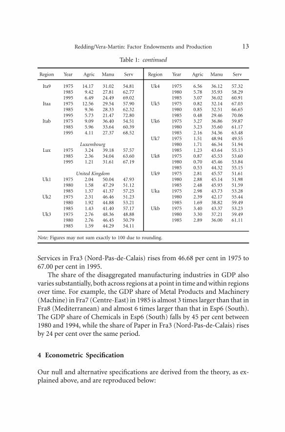
Table 1 presents information on the share of the three aggregate in-dustries in each region’s GDP in 1975, 1985 and 1995. We find substantialvariation in patterns of production across regions at any one point in time,even at the level of the three aggregate industries. For example, the share ofAgriculture in GDP in 1985 varies from 0.03 per cent in Be1 (Brussels) to11.86 per cent in Esp4 (Centre), while the GDP share of Services in the sameyear ranges from 81.61 per cent in Be1 (Brussels) to 49.57 per cent in Esp2(North East). There are also marked changes in patterns of specializationover time. Thus, the GDP share of Agriculture in Esp4 (Centre) falls from14.72 per cent in 1980 to 5.39 per cent in 1995, while the GDP share of

9 We also experiment with using data on arable land area to control for variation in landquality.10 See Appendix A for further information concerning the data used.

12 Review of World Economics 2006, Vol. 142 (1)

Table 1: Shares of Agriculture, Manufacturing and Services in GDP (per cent)

Region Year Agric Manu Serv Region Year Agric Manu Serv

Belgium Fra6 1975 8.57 37.15 54.28Be1 1975 0.01 28.58 71.42 1985 6.67 30.56 62.77

1985 0.03 18.35 81.61 1995 4.41 24.37 71.221995 0.02 15.75 84.23 Fra7 1975 4.30 46.46 49.24

Be2 1975 3.64 42.45 53.92 1985 3.11 36.85 60.041985 2.64 37.39 59.96 1995 2.43 32.17 65.401995 1.52 34.27 64.21 Fra8 1975 5.98 32.96 61.06

Be3 1975 3.91 39.93 56.16 1985 4.27 25.21 70.521985 3.00 32.24 64.76 1995 3.24 20.26 76.511995 1.76 27.36 70.88

NetherlandsSpain Nld1 1975 7.55 36.91 55.54

Esp1 1980 9.35 39.22 51.43 1985 4.33 35.08 60.581985 8.07 39.29 52.64 1995 4.45 38.53 57.021995 4.82 34.45 60.73 Nld2 1975 7.24 35.21 57.55

Esp2 1980 5.93 48.12 45.95 1985 6.12 29.77 64.111985 4.59 45.84 49.57 1995 4.19 27.24 68.581995 2.25 42.12 55.63 Nld3 1975 3.73 32.48 63.80

Esp3 1980 0.55 30.58 68.86 1985 3.29 28.23 68.481985 0.32 28.61 71.08 1995 2.71 23.64 73.651995 0.17 25.26 74.57 Nld4 1975 4.70 43.21 52.09

Esp4 1980 14.72 34.61 50.67 1985 5.48 37.25 57.271985 11.86 36.10 52.04 1995 3.55 32.62 63.831995 5.39 34.50 60.11

Esp5 1980 4.24 42.19 53.56 Italy1985 3.00 39.44 57.56 Ita1 1975 4.46 48.20 47.341995 1.57 34.55 63.87 1985 3.12 41.17 55.71

Esp6 1980 10.91 33.13 55.97 1995 2.42 36.87 60.711985 10.84 29.25 59.91 Ita2 1975 2.87 55.18 41.951995 6.15 27.91 65.95 1985 2.05 45.49 52.45

Esp7 1980 8.25 21.38 70.37 1995 1.56 41.21 57.231985 4.80 18.41 76.79 Ita3 1975 6.03 45.82 48.151995 2.06 18.56 79.38 1985 4.38 40.96 54.66

1995 3.13 36.71 60.17France Ita4 1975 8.72 47.13 44.15

Fra1 1975 0.68 34.87 64.45 1985 5.75 40.87 53.381985 0.40 29.50 70.10 1995 3.70 36.94 59.361995 0.18 22.54 77.28 Ita5 1975 5.32 45.34 49.34

Fra2 1975 8.73 43.58 47.69 1985 3.36 41.09 55.551985 7.41 36.07 56.52 1995 2.64 34.62 62.751995 4.27 32.69 63.04 Ita6 1975 4.40 26.02 69.57

Fra3 1975 4.04 49.28 46.68 1985 2.59 25.09 72.321985 2.62 35.80 61.58 1995 1.62 21.24 77.141995 1.35 31.66 67.00 Ita7 1975 10.70 39.19 50.11

Fra4 1975 4.45 47.50 48.05 1985 6.72 34.32 58.951985 3.71 37.48 58.81 1995 4.53 32.04 63.431995 2.60 34.66 62.74 Ita8 1975 10.26 31.29 58.45

Fra5 1975 11.38 37.48 51.14 1985 5.38 27.71 66.911985 7.98 29.24 62.78 1995 3.33 24.30 72.361995 5.24 27.08 67.69

Redding/Vera-Martin: Factor Endowments and Production 13

Table 1: continued

Region Year Agric Manu Serv Region Year Agric Manu Serv

Ita9 1975 14.17 31.02 54.81 Uk4 1975 6.56 36.12 57.321985 9.42 27.81 62.77 1980 5.78 35.93 58.291995 6.49 24.49 69.02 1985 3.07 36.02 60.91

Itaa 1975 12.56 29.54 57.90 Uk5 1975 0.82 32.14 67.031985 9.36 28.33 62.32 1980 0.85 32.51 66.651995 5.73 21.47 72.80 1985 0.48 29.46 70.06

Itab 1975 9.09 36.40 54.51 Uk6 1975 3.27 36.86 59.871985 5.96 33.64 60.39 1980 3.23 35.60 61.171995 4.11 27.37 68.52 1985 2.16 34.36 63.48

Uk7 1975 1.51 48.94 49.55Luxembourg 1980 1.71 46.34 51.94

Lux 1975 3.24 39.18 57.57 1985 1.23 43.64 55.131985 2.36 34.04 63.60 Uk8 1975 0.87 45.53 53.601995 1.21 31.61 67.19 1980 0.70 45.46 53.84

1985 0.53 44.32 55.15United Kingdom Uk9 1975 2.81 45.57 51.61

Uk1 1975 2.04 50.04 47.93 1980 2.88 45.14 51.981980 1.58 47.29 51.12 1985 2.48 45.93 51.591985 1.37 41.37 57.25 Uka 1975 2.98 43.73 53.28

Uk2 1975 2.31 46.46 51.23 1980 2.39 42.17 55.441980 1.92 44.88 53.21 1985 1.69 38.82 59.491985 1.43 41.40 57.17 Ukb 1975 3.40 43.37 53.23

Uk3 1975 2.76 48.36 48.88 1980 3.30 37.21 59.491980 2.76 46.45 50.79 1985 2.89 36.00 61.111985 1.59 44.29 54.11

Note: Figures may not sum exactly to 100 due to rounding.

Services in Fra3 (Nord-Pas-de-Calais) rises from 46.68 per cent in 1975 to67.00 per cent in 1995.

The share of the disaggregated manufacturing industries in GDP alsovaries substantially, both across regions at a point in time and within regionsover time. For example, the GDP share of Metal Products and Machinery(Machine) in Fra7 (Centre-East) in 1985 is almost 3 times larger than that inFra8 (Mediterranean) and almost 6 times larger than that in Esp6 (South).The GDP share of Chemicals in Esp6 (South) falls by 45 per cent between1980 and 1994, while the share of Paper in Fra3 (Nord-Pas-de-Calais) risesby 24 per cent over the same period.

4 Econometric Specification

Our null and alternative specifications are derived from the theory, as ex-plained above, and are reproduced below:

14 Review of World Economics 2006, Vol. 142 (1)

(NULL) szjt =∑

iγji ln vzit + ∑

tφjtdt + εzjt

(ALT1) szjt =∑

iγji ln vzit + ∑

tφjtdt + ηcj + εzjt

(ALT2) szjt =∑

iγji ln vzit + ∑

tφjtdt + ∑

c �=c′

∑

tµcjtdct + εzjt

(ALT3) szjt =∑

iγji ln vzit + ∑

tφjtdt + ∑

c �=c′

∑

tµcjtdct

+ ηzj + εzjt .

Since all coefficients vary across industries, the specifications are estimatedseparately for each industry, pooling observations across regions and overtime. Standard errors reported below are heteroscedasticity-robust and ad-justed for clustering on country-year.

As we start from (NULL) and move to (ALT3), we consider progressivelymore general models. However, in moving from (ALT2) to (ALT3), thewithin groups transformation due to the inclusion of the regional fixed effect(ηzj) can greatly exacerbate any attenuation bias from measurement errorin the independent variables (see, in particular, Griliches and Hausman1986). Intuitively, the extent of ‘within’ or time-series variation in factorendowments due to true variation in the independent variables may besmall relative to the variation due to measurement error. This is likely tobe a particular problem in the present application because the extent oftime-series variation in some of our factor endowments (in particular landarea and, to a lesser extent, population) is limited.

We address this problem in two ways. First, we exploit disaggregateddata on the educational attainment of the population and on arable landarea. The resulting measures of factor endowments control for variationin levels of skills and land quality, and exhibit greater differential vari-ation over time within regions. Second, following Griliches and Hausman(1986), we consider the use of first-differenced estimators. The longerthe interval of time over which we difference the data, the greater theamount of true variation in factor endowments relative to that due tomeasurement error. Hence, the attenuation bias due to measurement errorshould be smaller using longer differences, and we analyse the results of10-year difference estimators. We thus obtain a fourth alternative specifi-cation:

(ALT4) �10szjt = ∑

iγji�10 ln vzit + ∑

tζjtdt + ψzjt , (7)

Redding/Vera-Martin: Factor Endowments and Production 15

where differencing eliminates the regional fixed effect (ηzj). In taking longdifferences, we substantially reduce the sample size and, therefore, we con-centrate on a specification including time dummies that are common acrosscountries together with their industry-specific coefficients.

In comparing the results of estimating the null and alternative specifi-cations, we also make use of two model specification tests. The first of thesefocuses on the time-series properties of the model. By construction, theshare of sector j in GDP (szjt) is bounded between 0 and 100 per cent, and istherefore I(0). However, in any finite sample, GDP shares may be I(1). Thisis particularly true of our sample period (1975–1995) which, in general,is characterized by a secular decline in the GDP shares of Agriculture andManufacturing combined with a secular rise in the share of Services. Simi-larly, a region’s population and physical capital endowments may be I(1). Inthis case, the static-level regressions (NULL)–(ALT3) should be interpretedas cointegrating relationships between a sector’s share of GDP and factorendowments. Under this interpretation, the residuals should be I(0) if theassumptions underlying a particular specification are satisfied. Therefore,we make use of recent advances in panel data unit root tests, exploitingthe Maddala and Wu (1999) methodology to test for the stationarity of theresiduals.11

Second, neoclassical trade theory assumes that the production tech-nology is constant returns to scale, implying that the revenue function inequation (1) is homogenous of degree one in factor endowments, and im-plying that the industry share equation (2) is homogenous of degree zero infactor endowments. Therefore, a test of the null hypothesis that the sum ofthe estimated coefficients on factor endowments is equal to zero in speci-fications (NULL) and (ALT1)–(ALT4),

∑

iγji = 0, provides another model

specification test.

11 The Maddala and Wu or Fisher test statistic is based on the sum of the p-values fromconventional Augmented Dickey–Fuller (ADF) tests on the residuals for each cross-sectionunit z ∈ Z. It can be shown that −2

∑z ln Pz has a χ2 distribution with 2Z degrees of free-

dom. This test statistic has a direct intuitive interpretation, is valid for unbalanced panelsand has attractive small sample properties (Maddala and Wu 1999). Other analyses of unitroots and cointegration in a panel data context include Im et al. (2003), Levin and Lin(1992), Pedroni (1999), Pesaran et al. (1999) and Quah (1994).

16 Review of World Economics 2006, Vol. 142 (1)

5 Empirical Results

5.1 Aggregate Industries, Aggregate Endowments

We begin in column (1) of Table 2 by reporting the results of estimat-ing the HO specification (NULL) for the aggregate industries (Agriculture,Manufacturing and Services) using our three broad measures of factorendowments (population, physical capital and land area). We find a rela-tionship between regional patterns of production and factor endowmentswhich is statistically significant at the 5 per cent level and, from the regres-sion R2, the HO specification explains some 30–45 per cent of the variationin production patterns across European regions.

In column (2) of Table 2 (panels A–C), we relax the assumption of iden-tical relative prices and technology, and move to specification (ALT1). Thecountry-industry fixed effects, which are excluded from the null hypothesis,are highly statistically significant as shown in the first of the F-statisticsreported towards the bottom of the column. The R2 of the regression risessubstantially, and by more than one-third in both Agriculture and Manu-facturing. The pattern of estimated coefficients on factor endowments alsochanges and moves more in line with economic priors concerning factorintensity. For example, in Agriculture the coefficient on physical capitalswitches from being positive and statistically significant to negative andstatistically significant, while in Manufacturing the coefficients on physicalcapital and population increase by an order of magnitude.

Therefore, the strict version of the Heckscher–Ohlin model that assumesidentical relative prices and technology is rejected against more generalalternatives. The country-industry fixed effects are not only statisticallysignificant but also quantitatively important, as reflected in the rise in theregression R2. The change in the pattern of estimated coefficients whenmoving from (NULL) to (ALT1) indicates that these additional controls areimportant for identifying the nature of the relationship between productionstructure and factor endowments.

In column (3) of Table 2 (panels A–C), we consider the more generalalternative specification (ALT2). We allow for differential movements acrosscountries and over time in relative prices, technology and other variablesomitted from the HO model by including a set of country-year dummies ineach industry regression for all countries except the base country c′. Fromthe first of the F-statistics reported towards the bottom of this column, thecoefficients on the country-year dummies are highly statistically significant

Redding/Vera-Martin: Factor Endowments and Production 17Ta

ble

2:Fa

ctor

Endo

wm

ents

and

Spec

ializ

atio

nin

Thr

eeA

ggre

gate

Sect

ors

(1)

(2)

(3)

(4)

(1)

(2)

(3)

(4)

(1)

(2)

(3)

(4)

811

obs.

811

obs.

811

obs.

811

obs.

811

obs.

811

obs.

811

obs.

811

obs.

811

obs.

811

obs.

811

obs.

811

obs.

1975

-95

1975

-95

1975

-95

1975

-95

1975

-95

1975

-95

1975

-95

1975

-95

1975

-95

1975

-95

1975

-95

1975

-95

A.

Agr

icul

ture

B.

Man

ufac

turi

ngC

.Se

rvic

esC

apit

al0.

004∗

−0.0

22∗∗

−0.0

19∗∗

0.01

1∗∗

−0.0

050.

071∗

∗0.

073∗

∗0.

043∗

∗0.

001

−0.0

49∗∗

−0.0

54∗∗

−0.0

54∗∗

(0.0

024)

(0.0

050)

(0.0

055)

(0.0

045)

(0.0

058)

(0.0

205)

(0.0

241)

(0.0

080)

(0.0

045)

(0.0

163)

(0.0

196)

(0.0

097)

Popu

lati

on−0

.021

∗∗0.

002

−0.0

02−0

.129

∗∗−0

.008

−0.0

79∗∗

−0.0

82∗∗

0.20

5∗∗

0.02

9∗∗

0.07

8∗∗

0.08

3∗∗

−0.0

76∗∗

(0.0

025)

(0.0

050)

(0.0

054)

(0.0

216)

(0.0

063)

(0.0

195)

(0.0

231)

(0.0

384)

(0.0

055)

(0.0

158)

(0.0

191)

(0.0

313)

Lan

d0.

017∗

∗0.

016∗

∗0.

016∗

∗−0

.055

∗∗0.

021∗

∗0.

032∗

∗0.

033∗

∗−0

.130

−0.0

38∗∗

−0.0

48∗∗

−0.0

48∗∗

0.18

5∗∗

(0.0

009)

(0.0

011)

(0.0

012)

(0.0

199)

(0.0

019)

(0.0

033)

(0.0

037)

(0.0

945)

(0.0

018)

(0.0

031)

(0.0

035)

(0.0

797)

Sam

ple

AA

AA

AA

AA

AA

AA

Spec

ifica

tion

(NU

LL

)(A

LT1)

(ALT

2)(A

LT3)

(NU

LL

)(A

LT1)

(ALT

2)(A

LT3)

(NU

LL

)(A

LT1)

(ALT

2)(A

LT3)

Year

dum

mie

sye

sye

sye

sye

sye

sye

sC

oun

try

effe

cts

yes

yes

yes

Cty

-yea

rdu

mm

ies

yes

yes

yes

yes

yes

yes

Reg

ion

effe

cts

yes

yes

yes

Pro

b>F(

NU

LL–

ALT

)N

/A

0.00

000.

0000

0.00

00N

/A

0.00

000.

0000

0.00

00N

/A0.

0000

0.00

000.

0000

Pro

b>F(

AL

L)

0.00

000.

0000

0.00

000.

0000

0.00

000.

0000

0.00

000.

0000

0.00

000.

0000

0.00

000.

0000

R-s

quar

ed0.

400.

630.

650.

960.

290.

400.

420.

970.

450.

530.

550.

98Su

mof

coef

f.0.

0003

−0.0

046

−0.0

050

−0.1

730

0.00

820.

0239

0.02

400.

1180

−0.0

085

−0.0

192

−0.0

190.

055

Lin

ear

hom

og.

(0.7

707)

(0.0

000)

(0.0

001)

(0.0

000)

(0.0

168)

(0.0

001)

(0.0

002)

(0.2

763)

(0.0

178)

(0.0

005)

(0.0

011)

(0.5

373)

(p-v

alu

e)ac

cept

reje

ctre

ject

reje

ctre

ject

reje

ctre

ject

acce

ptre

ject

reje

ctre

ject

acce

ptM

adda

la–W

u(0

.018

8)(0

.038

9)(0

.026

3)(0

.000

2)(0

.004

0)(0

.002

0)(0

.194

9)(0

.177

9)(0

.170

5)(0

.246

0)(0

.046

4)(0

.411

5)(p

-val

ue)

reje

ctre

ject

reje

ctre

ject

reje

ctre

ject

acce

ptac

cept

acce

ptac

cept

reje

ctac

cept

Not

e:P

rob>

F(N

UL

L–A

LT)

isth

ep-

valu

efo

ran

F-t

est

ofth

en

ull

hypo

thes

isth

atth

eco

effi

cien

tson

the

vari

able

sex

clu

ded

from

spec

ifica

tion

(NU

LL

)bu

tin

cude

din

the

alte

rnat

ive

spec

ifica

tion

are

equ

alto

0.P

rob>

F(A

LL

)is

the

p-va

lue

for

the

conv

enti

onal

F-t

est

that

the

coef

fici

ents

onal

lin

depe

nde

nt

vari

able

sar

eeq

ual

toze

ro.

Sum

ofco

eff.

isth

esu

mof

the

esti

mat

edco

effi

cien

tson

fact

oren

dow

men

ts.

Lin

ear

hom

og.

isth

ep-

valu

efo

ra

test

ofth

en

ull

hypo

thes

isth

atth

esu

mof

the

esti

mat

edco

effi

cien

tson

fact

oren

dow

men

tsis

equ

alto

zero

.M

adda

la–W

uis

the

p-va

lue

for

the

Mad

dala

and

Wu

(199

9)pa

nel

data

test

ofth

en

ull

hypo

thes

isth

atth

ere

sidu

als

hav

ea

un

itro

ot.

Stan

dard

erro

rsin

pare

nth

eses

are

het

eros

ceda

stic

ity-

robu

stan

dcl

ust

ered

onco

un

try-

year

.∗∗

den

otes

sign

ifica

nce

atth

e5

per

cen

tle

vel,

∗ den

otes

sign

ifica

nce

atth

e10

per

cen

tle

vel.

18 Review of World Economics 2006, Vol. 142 (1)

in all industries, providing further evidence against the HO null hypo-thesis.

Comparing columns (2) and (3), the pattern of estimated coefficientson factor endowments remains stable between specifications (ALT1) and(ALT2). This suggests that controlling for different cross-country trends inrelative prices, technology and other omitted variables does not substantiallyalter the relationship between factor endowments and regional productionpatterns, and that it is more important to control for time-invariant cross-country differences in relative prices, technology and other omitted variablesin the move from (NULL) to (ALT1).

The values of the estimated coefficients on factor endowments in (ALT2)are generally consistent with economic priors. Population endowments arepositively correlated with specialization in Services and negatively corre-lated with specialization in Manufacturing. Greater endowments of phys-ical capital are associated with a higher share of Manufacturing in GDPand a lower share of Agriculture and Services. Land area is positively re-lated to specialization in Agriculture and Manufacturing and negativelyrelated to specialization in Services. With the exception of the coefficient onpopulation in the regression for Agriculture, all estimated coefficients arestatistically significant at the 5 per cent level.

Column (4) of Table 2 (panels A–C) reports the results of extendingthe model further to include a region-industry fixed effect in specification(ALT3). Here, the pattern of estimated coefficients changes substantiallyand no longer has a plausible economic interpretation. For example, landarea is negatively correlated with the share of Agriculture in GDP, whileendowments of physical capital are positively and statistically significantlycorrelated with specialization in Agriculture. Since there is almost no time-series variation in land area, and any variation reflects either the reclamationof areas from the sea (the Netherlands) or measurement error, it is unclearhow appropriate or meaningful this econometric specification is. The pa-rameters of interest are being identified from deviations from time meansfor individual regions, which in all cases are extremely small and in manycases are literally zero. It is plausible that the change in the estimated coeffi-cients between (ALT2) and (ALT3) is largely driven by measurement error(Griliches and Hausman 1986). We investigate this possibility further below,where we disaggregate factor endowments (thereby introducing more time-series variation) and explore the results of long differences estimation.

Table 2 also reports the sum of the estimated coefficients on factorendowments in each industry and the results of a test whether the revenue

Redding/Vera-Martin: Factor Endowments and Production 19

function is linearly homogenous of degree 1 in factor endowments (a testof the null hypothesis that

∑i γji = 0). Although the sum of the estimated

coefficients is close to zero (in several cases in the order of magnitude of10−2), the null hypothesis is frequently rejected at conventional levels ofstatistical significance. There is some evidence of increasing returns to scalein Manufacturing, where the sum of the estimated coefficients is strictlygreater than zero in all specifications.

Our other model specification test examines the stationarity of the resid-uals using the panel data unit root tests of Maddala and Wu (1999). InAgriculture we are able to reject the null hypothesis of a unit root in theresiduals in all specifications, while in Services and Manufacturing we areunable to reject the null hypothesis in half the specifications. Taken together,these results provide some evidence of model misspecification. Two possibleexplanations for the non-stationarity of the residuals are, first, the omissionof information on relevant factor endowments and, second, region-timevariation in relative prices, technology and other omitted variables thathave not been controlled for (and which will therefore be included in theerror term).

5.2 Aggregate Industries, Disaggregate Endowments

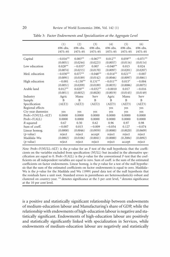
Table 3 investigates the first of these possibilities by introducing informa-tion on educational attainment and land quality. The availability of theeducational attainment data reduces the sample size to 696 observationsper industry (Sample B).12 In the interest of brevity, we only report theresults for specifications (ALT2) and (ALT3). In both cases, as shown in thefirst F-statistic reported in the table, we reject the HO null against the moregeneral alternative, and we begin by considering the estimation results forspecification (ALT2).

The estimated coefficients on physical capital are very similar to thosebefore, while the arable land coefficients closely resemble those on total landarea. In addition, we find highly statistically significant effects of educationendowments. Greater endowments of low-education labour are positivelyand statistically significantly correlated with specialization in Agriculture,while endowments of medium-education labour are negatively and statis-tically significantly correlated with the share of Agriculture in GDP. There

12 The model in Table 2 (panels A–C) was re-estimated for the reduced sample; this yieldsvery similar results to those reported in the paper.

20 Review of World Economics 2006, Vol. 142 (1)

Table 3: Factor Endowments and Specialization at the Aggregate Level

(1) (2) (3) (4) (5) (6)696 obs. 696 obs. 696 obs. 696 obs. 696 obs. 696 obs.1975–95 1975–95 1975–95 1975–95 1975–95 1975–95

Capital −0.016∗∗ 0.083∗∗ −0.067∗∗ 0.012∗∗ 0.059∗∗ −0.071∗∗(0.0051) (0.0244) (0.0223) (0.0057) (0.0116) (0.0114)

Low education 0.028∗∗ −0.035∗ 0.007 −0.040∗∗ 0.015 0.024(0.0074) (0.0215) (0.0170) (0.0097) (0.0201) (0.0207)

Med. education −0.030∗∗ 0.077∗∗ −0.048∗∗ −0.014∗∗ 0.021∗∗ −0.007(0.0091) (0.0189) (0.0142) (0.0046) (0.0097) (0.0061)

High education −0.001 −0.130∗∗ 0.131∗∗ −0.011∗∗ 0.015∗ −0.004(0.0051) (0.0209) (0.0189) (0.0035) (0.0086) (0.0075)

Arable land 0.012∗∗ 0.020∗∗ −0.032∗∗ −0.0010 0.017 −0.016(0.0011) (0.0032) (0.0028) (0.0019) (0.0145) (0.0149)

Industry Agric Manu Serv Agric Manu ServSample B B B B B BSpecification (ALT2) (ALT2) (ALT2) (ALT3) (ALT3) (ALT3)Regional effects yes yes yesCty-year dummies yes yes yes yes yes yesProb>F(NULL–ALT) 0.0000 0.0000 0.0000 0.0000 0.0000 0.0000Prob>F(ALL) 0.0000 0.0000 0.0000 0.0000 0.0000 0.0000R-squared 0.67 0.50 0.62 0.96 0.97 0.98Sum of coeff. −0.007 0.015 −0.009 −0.054 0.127 −0.074Linear homog. (0.0000) (0.0046) (0.0959) (0.0000) (0.0020) (0.0609)(p-value) reject reject accept reject reject rejectMaddala–Wu (0.0002) (0.0106) (0.0041) (0.0000) (0.2084) (0.0092)(p-value) reject reject reject reject accept reject

Note: Prob>F(NULL–ALT) is the p-value for an F-test of the null hypothesis that the coeffi-cients on the variables excluded from specification (NULL) but incuded in the alternative spe-cification are equal to 0. Prob>F(ALL) is the p-value for the conventional F-test that the coef-ficients on all independent variables are equal to zero. Sum of coeff. is the sum of the estimatedcoefficients on factor endowments. Linear homog. is the p-value for a test of the null hypothe-sis that the sum of the estimated coefficients on factor endowments is equal to zero. Maddala–Wu is the p-value for the Maddala and Wu (1999) panel data test of the null hypothesis thatthe residuals have a unit root. Standard errors in parentheses are heteroscedasticity-robust andclustered on country-year. ∗∗ denotes significance at the 5 per cent level, ∗ denotes significanceat the 10 per cent level.

is a positive and statistically significant relationship between endowmentsof medium-education labour and Manufacturing’s share of GDP, while therelationship with endowments of high-education labour is negative and sta-tistically significant. Endowments of high-education labour are positivelyand statistically significantly linked with specialization in Services, whileendowments of medium-education labour are negatively and statistically

Redding/Vera-Martin: Factor Endowments and Production 21

significantly linked with the share of Services in GDP. This pattern of resultsis consistent with the idea that Services is skilled-labour-intensive relativeto Agriculture and Manufacturing.

The introduction of more disaggregated measures of factor endowmentsincreases the regression R2, which in Manufacturing rises from 0.42 incolumn (3) of Table 2B to 0.50 in column (2) of Table 3. Furthermore, weare now able to reject the null hypothesis of a unit root in the residuals at the5 per cent level in all three industries. This is consistent with the idea thatthe non-stationarity of the residuals in the specification with population,physical capital and land area was due to the omission of information onrelevant factor endowments. The sum of the estimated coefficients on factorendowments in all three industries is again close to zero, although the nullhypothesis that the revenue function is linearly homogenous of degree 1 istypically rejected at the 5 per cent level. The sum of the estimated coefficientsin Manufacturing remains strictly greater than zero, again providing someevidence of increasing returns to scale.

The introduction of the region-industry fixed effects in (ALT3) againleads to a change in the estimated pattern of coefficients which often nolonger have a plausible economic interpretation. For example, increases inarable land area are negatively (though not statistically significantly) relatedto specialization in Agriculture. Again, it is plausible that these results aredriven by measurement error—the extent of true time-series variation infactor endowments within regions still remains small relative to that due tomeasurement error, and this is particularly the case for arable land area.

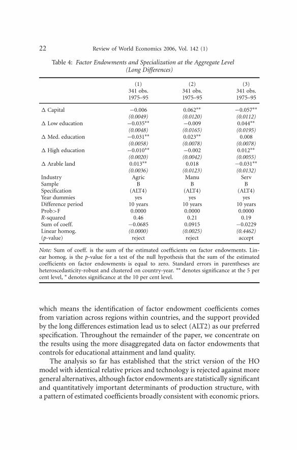
Table 4 investigates this possibility further using the results of long dif-ferences estimation over a 10-year time period (ALT4). The long differencesestimator enables us to control for unobserved heterogeneity at the regionallevel, while reducing the magnitude of any attenuation bias induced bymeasurement error. The pattern of estimated coefficients in Table 4 is simi-lar to that reported for (ALT2) in Table 3. For example, arable land area ispositively and statistically significantly correlated with the share of Agricul-ture in GDP and negatively and statistically significantly correlated with theshare of Services. The main exception is for the low-education endowmentwhere one of the estimated coefficients changes sign.13

The constancy of the estimated parameters as one moves from (ALT1)to (ALT2) in Table 2, the inclusion of country-year dummies in (ALT2)

13 We also experimented with differencing over six- and eight-year time periods whichyielded a broadly similar pattern of results.

22 Review of World Economics 2006, Vol. 142 (1)

Table 4: Factor Endowments and Specialization at the Aggregate Level(Long Differences)

(1) (2) (3)341 obs. 341 obs. 341 obs.1975–95 1975–95 1975–95

∆ Capital −0.006 0.062∗∗ −0.057∗∗(0.0049) (0.0120) (0.0112)

∆ Low education −0.035∗∗ −0.009 0.044∗∗(0.0048) (0.0165) (0.0195)

∆ Med. education −0.031∗∗ 0.023∗∗ 0.008(0.0058) (0.0078) (0.0078)

∆ High education −0.010∗∗ −0.002 0.012∗∗(0.0020) (0.0042) (0.0055)

∆ Arable land 0.013∗∗ 0.018 −0.031∗∗(0.0036) (0.0123) (0.0132)

Industry Agric Manu ServSample B B BSpecification (ALT4) (ALT4) (ALT4)Year dummies yes yes yesDifference period 10 years 10 years 10 yearsProb>F 0.0000 0.0000 0.0000R-squared 0.46 0.21 0.19Sum of coeff. −0.0685 0.0915 −0.0229Linear homog. (0.0000) (0.0025) (0.4462)(p-value) reject reject accept

Note: Sum of coeff. is the sum of the estimated coefficients on factor endowments. Lin-ear homog. is the p-value for a test of the null hypothesis that the sum of the estimatedcoefficients on factor endowments is equal to zero. Standard errors in parentheses areheteroscedasticity-robust and clustered on country-year. ∗∗ denotes significance at the 5 percent level, ∗ denotes significance at the 10 per cent level.

which means the identification of factor endowment coefficients comesfrom variation across regions within countries, and the support providedby the long differences estimation lead us to select (ALT2) as our preferredspecification. Throughout the remainder of the paper, we concentrate onthe results using the more disaggregated data on factor endowments thatcontrols for educational attainment and land quality.

The analysis so far has established that the strict version of the HOmodel with identical relative prices and technology is rejected against moregeneral alternatives, although factor endowments are statistically significantand quantitatively important determinants of production structure, witha pattern of estimated coefficients broadly consistent with economic priors.

Redding/Vera-Martin: Factor Endowments and Production 23

5.3 Disaggregate Industries, Disaggregate Endowments

In this section, we examine whether factor endowments are more or lesssuccessful in explaining specialization in disaggregated industries within themanufacturing sector than in the aggregate industries we have consideredabove. It is often argued in the literature on imperfect competition andtrade (e.g. Helpman and Krugman 1985) that other considerations such asimperfect competition and increasing returns to scale are more importantfor production and trade within Manufacturing.

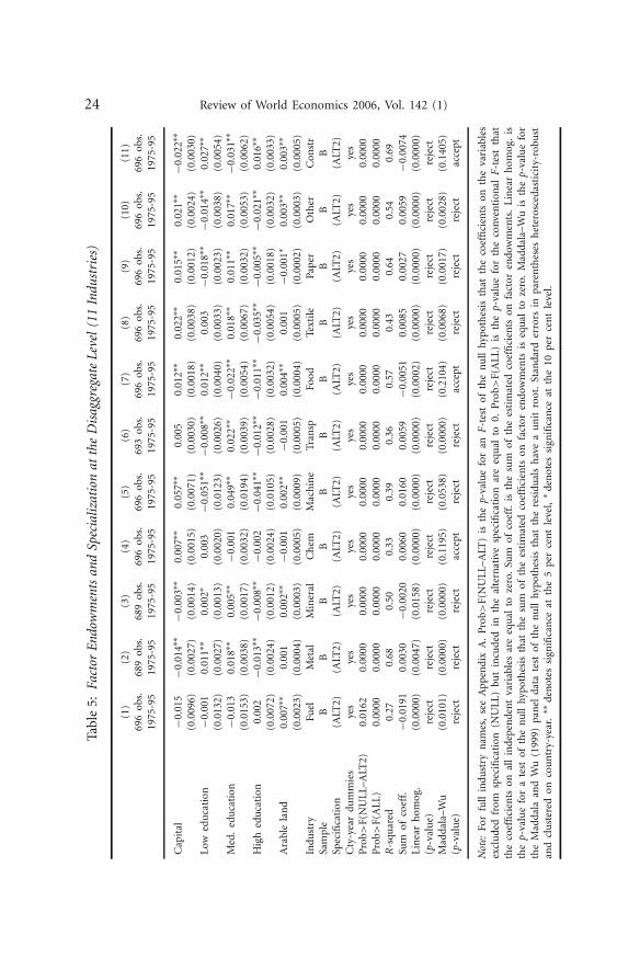
Table 5 reports the results of estimating our preferred specification(ALT2) with the five factor endowments for 11 disaggregated manufac-turing industries, including Fuels, Ferrous Metals, Non-metallic Minerals,Chemicals, Machinery, Transport Equipment, Food Beverages & Tobacco,Textiles, Paper & Printing, Building & Construction, and MiscellaneousOther Production.

Factor endowments are again found to play a statistically significant rolein explaining production structure, and the general equilibrium effects offactor endowments on production in individual industries vary substan-tially within manufacturing. Physical capital is positively and statisticallysignificantly related to the share of Chemicals and Machinery in a region’sGDP. Medium-education is positively and statistically significantly corre-lated with specialization in Metals, Machinery and Transport Equipment.

In all industries, the HO specification (NULL) is rejected against themore general alternative (ALT2) at the 5 per cent level of statistical signifi-cance, as shown in the first of the F-statistics reported towards the bottom ofeach column and panel of the table. The contributions of the country-yeardummies are again not only statistically significant but also quantitativelyimportant, with the regression R2 in each industry rising markedly betweenspecifications (NULL) and (ALT2).

In Table 6 we examine the predictive power of the model at different levelsof industrial disaggregation by calculating within-sample average absoluteprediction errors. These are defined in proportional terms as

∣∣szjt − szjt

∣∣/szjt ,

where a hat above a variable indicates a predicted value.14

For the three aggregate industries of Agriculture, Manufacturing andServices, we find that the HO specification (NULL) provides a relatively

14 The model’s predictions for output levels can be obtained by multiplying predictedGDP shares by actual GDP. Proportional prediction errors for output are therefore exactlythe same as for shares of sectors in GDP (one is multiplying both the numerator and de-nominator of the formula in the text by actual GDP).

24 Review of World Economics 2006, Vol. 142 (1)Ta

ble

5:Fa

ctor

Endo

wm

ents

and

Spec

ializ

atio

nat

the

Dis

aggr

egat

eLe

vel

(11

Indu

stri

es)

(1)

(2)

(3)

(4)

(5)

(6)

(7)

(8)

(9)

(10)

(11)

696

obs.

689

obs.

689

obs.

696

obs.

696

obs.

693

obs.

696

obs.

696

obs.

696

obs.

696

obs.

696

obs.

1975

-95

1975

-95

1975

-95

1975

-95

1975

-95

1975

-95

1975

-95

1975

-95

1975

-95

1975

-95

1975

-95

Cap

ital

−0.0

15−0

.014

∗∗−0

.003

∗∗0.

007∗

∗0.

057∗

∗0.

005

0.01

2∗∗

0.02

2∗∗

0.01

5∗∗

0.02

1∗∗

−0.0

22∗∗

(0.0

096)

(0.0

027)

(0.0

014)

(0.0

015)

(0.0

071)

(0.0

030)

(0.0

018)

(0.0

038)

(0.0

012)

(0.0

024)

(0.0

030)

Low

edu

cati

on−0

.001

0.01

1∗∗

0.00

2∗0.

003

−0.0

51∗∗

−0.0

08∗∗

0.01

2∗∗

0.00

3−0

.018

∗∗−0

.014

∗∗0.

027∗

∗(0

.013

2)(0

.002

7)(0

.001

3)(0

.002

0)(0

.012

3)(0

.002

6)(0

.004

0)(0

.003

3)(0

.002

3)(0

.003

8)(0

.005

4)M

ed.

edu

cati

on−0

.013

0.01

8∗∗

0.00

5∗∗

−0.0

010.

049∗

∗0.

022∗

∗−0

.022

∗∗0.

018∗

∗0.

011∗

∗0.

017∗

∗−0

.031

∗∗(0

.015

3)(0

.003

8)(0

.001

7)(0

.003

2)(0

.019

4)(0

.003

9)(0

.005

4)(0

.006

7)(0

.003

2)(0

.005

3)(0

.006

2)H

igh

edu

cati

on0.

002

−0.0

13∗∗

−0.0

08∗∗

−0.0

02−0

.041

∗∗−0

.012

∗∗−0

.011

∗∗−0

.035

∗∗−0

.005

∗∗−0

.021

∗∗0.

016∗

∗(0

.007

2)(0

.002

4)(0

.001

2)(0

.002

4)(0

.010

5)(0

.002

8)(0

.003

2)(0

.005

4)(0

.001

8)(0

.003

2)(0

.003

3)A

rabl

ela

nd

0.00

7∗∗

0.00

10.

002∗

∗−0

.001

0.00

2∗∗

−0.0

010.

004∗

∗0.

001

−0.0

01∗

0.00

3∗∗

0.00

3∗∗

(0.0

023)

(0.0

004)

(0.0

003)

(0.0

005)

(0.0

009)

(0.0

005)

(0.0

004)

(0.0

005)

(0.0

002)

(0.0

003)

(0.0

005)

Indu

stry

Fuel

Met

alM

iner

alC

hem

Mac

hin

eTr

ansp

Food

Text

ilePa

per

Oth

erC

onst

rSa

mpl

eB

BB

BB

BB

BB

BB

Spec

ifica

tion

(ALT

2)(A

LT2)

(ALT

2)(A

LT2)

(ALT

2)(A

LT2)

(ALT

2)(A

LT2)

(ALT

2)(A

LT2)

(ALT

2)C

ty-y

ear

dum

mie

sye

sye

sye

sye

sye

sye

sye

sye

sye

sye

sye

sP

rob>

F(N

UL

L–A

LT2)

0.01

620.

0000

0.00

000.

0000

0.00

000.

0000

0.00

000.

0000

0.00

000.

0000

0.00

00P

rob>

F(A

LL

)0.

0000

0.00

000.

0000

0.00

000.

0000

0.00

000.

0000

0.00

000.

0000

0.00

000.

0000

R-s

quar

ed0.

270.

680.

500.

330.

390.

360.

570.

430.

640.

540.

69Su

mof

coef

f.−0

.019

10.

0030

−0.0

020

0.00

600.

0160

0.00

59−0

.005

10.

0085

0.00

270.

0059

−0.0

074

Lin

ear

hom

og.

(0.0

000)

(0.0

047)

(0.0

158)

(0.0

000)

(0.0

000)

(0.0

000)

(0.0

002)

(0.0

000)

(0.0

000)

(0.0

000)

(0.0

000)

(p-v

alu

e)re

ject

reje

ctre

ject

reje

ctre

ject

reje

ctre

ject

reje

ctre

ject

reje

ctre

ject

Mad

dala

–Wu

(0.0

101)

(0.0

000)

(0.0

000)

(0.1

195)

(0.0

538)

(0.0

000)

(0.2

104)

(0.0

068)

(0.0

017)

(0.0

028)

(0.1

405)

(p-v

alu

e)re

ject

reje

ctre

ject

acce

ptre

ject

reje

ctac

cept

reje

ctre

ject

reje

ctac

cept

Not

e:Fo

rfu

llin

dust

ryn

ames

,se

eA

ppen

dix

A.

Pro

b>F(

NU

LL–

ALT

)is

the

p-va

lue

for

anF

-tes

tof

the

nu

llhy

poth

esis

that

the

coef

fici

ents

onth

eva

riab

les

excl

ude

dfr

omsp

ecifi

cati

on(N

UL

L)

but

incu

ded

inth

eal

tern

ativ

esp

ecifi

cati

onar

eeq

ual

to0.

Pro

b>F(

AL

L)

isth

ep-

valu

efo

rth

eco

nven

tion

alF

-tes

tth

atth

eco

effi

cien

tson

all

inde

pen

den

tva

riab

les

are

equ

alto

zero

.Su

mof

coef

f.is

the

sum

ofth

ees

tim

ated

coef

fici

ents

onfa

ctor

endo

wm

ents

.L

inea

rh

omog

.is

the

p-va

lue

for

ate

stof

the

nu

llhy

poth

esis

that

the

sum

ofth

ees

tim

ated

coef

fici

ents

onfa

ctor

endo

wm

ents

iseq

ual

toze

ro.

Mad

dala

–Wu

isth

ep-

valu

efo

rth

eM

adda

laan

dW

u(1

999)

pan

elda

tate

stof

the

nu

llhy

poth

esis

that

the

resi

dual

sh

ave

au

nit

root

.St

anda

rder

rors

inpa

ren

thes

esh

eter

osce

dast

icit

y-ro

bust

and

clu

ster

edon

cou

ntr

y-ye

ar.

∗∗de

not

essi

gnifi

can

ceat

the

5pe

rce

nt

leve

l,∗ de

not

essi

gnifi

can

ceat

the

10pe

rce

nt

leve

l.

Redding/Vera-Martin: Factor Endowments and Production 25

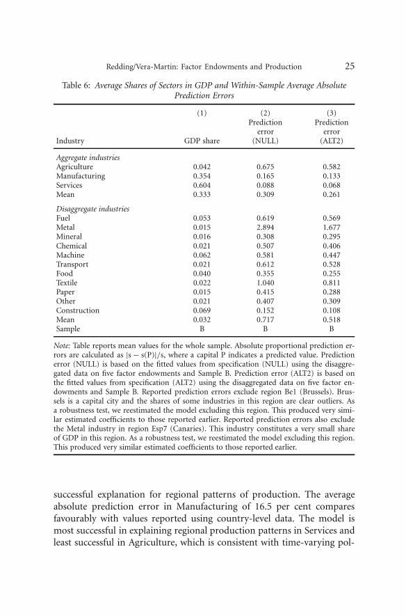
Table 6: Average Shares of Sectors in GDP and Within-Sample Average AbsolutePrediction Errors

(1) (2) (3)Prediction Prediction

error errorIndustry GDP share (NULL) (ALT2)

Aggregate industriesAgriculture 0.042 0.675 0.582Manufacturing 0.354 0.165 0.133Services 0.604 0.088 0.068Mean 0.333 0.309 0.261

Disaggregate industriesFuel 0.053 0.619 0.569Metal 0.015 2.894 1.677Mineral 0.016 0.308 0.295Chemical 0.021 0.507 0.406Machine 0.062 0.581 0.447Transport 0.021 0.612 0.528Food 0.040 0.355 0.255Textile 0.022 1.040 0.811Paper 0.015 0.415 0.288Other 0.021 0.407 0.309Construction 0.069 0.152 0.108Mean 0.032 0.717 0.518Sample B B B

Note: Table reports mean values for the whole sample. Absolute proportional prediction er-rors are calculated as |s − s(P)|/s, where a capital P indicates a predicted value. Predictionerror (NULL) is based on the fitted values from specification (NULL) using the disaggre-gated data on five factor endowments and Sample B. Prediction error (ALT2) is based onthe fitted values from specification (ALT2) using the disaggregated data on five factor en-dowments and Sample B. Reported prediction errors exclude region Be1 (Brussels). Brus-sels is a capital city and the shares of some industries in this region are clear outliers. Asa robustness test, we reestimated the model excluding this region. This produced very simi-lar estimated coefficients to those reported earlier. Reported prediction errors also excludethe Metal industry in region Esp7 (Canaries). This industry constitutes a very small shareof GDP in this region. As a robustness test, we reestimated the model excluding this region.This produced very similar estimated coefficients to those reported earlier.

successful explanation for regional patterns of production. The averageabsolute prediction error in Manufacturing of 16.5 per cent comparesfavourably with values reported using country-level data. The model ismost successful in explaining regional production patterns in Services andleast successful in Agriculture, which is consistent with time-varying pol-

26 Review of World Economics 2006, Vol. 142 (1)

icy interventions that have uneven effects across European regions beingimportant in Agriculture. The introduction of the country-year dummiesin our preferred specification (ALT2) leads to a reduction in the model’swithin-sample average absolute prediction error, with the greatest impactobserved in Agriculture.

Both the HO specification (NULL) and the alternative specification(ALT2) are less successful in explaining regional patterns of production indisaggregated industries within Manufacturing. Across the disaggregatedmanufacturing industries as a whole, the average absolute prediction errorrises to 71.7 per cent in specification (NULL) and 51.8 per cent in spe-cification (ALT2). The model is least successful in explaining patterns ofproduction in Metal Products (which includes Iron & Steel) and Textiles,both of which are again industries where historically there has been extensivepolicy intervention in Europe.

These findings of greater within-sample average absolute predictionerrors in disaggregated manufacturing industries are consistent with thelarger number of industries relative to factors of production at the disag-gregated level, suggesting the possibility of production indeterminacy. Theyare also consistent with the idea that omitted regional variation in relativeprices, technology or other determinants of production structure may beparticularly large in individual disaggregated manufacturing industries.

6 Conclusions

This paper has analysed the relationship between production structureand factor endowments using panel data on 14 industries in 45 regionsfrom 7 European countries since 1975. We derived a general equilibriumrelationship linking the share of a sector in GDP to factor endowments,relative prices and technology from the neoclassical model of trade. The HOmodel is a special case of this framework where relative prices and technologyare identical across regions. We compared the empirical performance of theHO null against a series of more general alternatives allowing for variationin relative prices, technology and other variables omitted from the HOmodel.

The use of European regional data enables us to abstract from manyof the considerations that have been proposed as explanations for the dis-appointing empirical performance of HO theory at the country level. Forexample, measurement error and technology differences are likely to be

Redding/Vera-Martin: Factor Endowments and Production 27

much smaller across regions within Europe than for a broad cross-sectionof developed and developing countries. The data also have the advantage ofincluding both manufacturing and non-manufacturing sectors, where thelatter play an important role in European regions, and we are able to explorethe model’s empirical performance for both broad and more finely detailedindustry classifications.

For both the three aggregate industries (Agriculture, Manufacturingand Services) and the 11 disaggregated industries within Manufacturing,the strict version of the HO model assuming identical relative prices andtechnology is rejected against more general alternatives. Nonetheless, factorendowments play a statistically significant and quantitatively important rolein explaining production structure in European regions, with a pattern ofestimated coefficients broadly consistent with economic priors.

The introduction of more disaggregated factor endowment measuresthat control for educational attainment and land quality leads to a substan-tial improvement in the model’s explanatory power. The HO null specifi-cation is more successful in explaining the production structure for broadindustries, such as Agriculture, Manufacturing and Services, than for morenarrowly defined industries within manufacturing. This is consistent witha larger number of industries relative to factors of production at the disag-gregate level, introducing the possibility of production indeterminacy, andwith the idea that omitted regional variation in relative prices, technologyor other determinants of production structure may be particularly large inindividual manufacturing industries.

Appendix A

Table A1: Sample Composition

Country Sample A Sample B Number of NUTS-1 regions

Belgium 1975–1995 1979–1995 3 (be1–be3)Spain 1980–1995 1980–1994 7 (esp1–esp7)France 1975–1995 1977–1994 8 (fra1–fra8)Italy 1975–1995 1980–1995 11 (ita1–ita9, itaa/b)Luxembourg 1975–1995 1979–1990 1 (lux)Netherlands 1975–1995 1977–1995 4 (ndl1–ndl4)United Kingdom 1975–1986 1975–1986 11 (uk1–uk9, uka/b)

28 Review of World Economics 2006, Vol. 142 (1)

Table A2: Industry Composition

Code Industry Description

Aggregate Industries1 Agricultural Sector: Food, Forestry and Fishery Products (Agric)2 Manufacturing Sector (Manu)3 Services Sector: Market Services (Serv)

Disaggregated Manufacturing Industries4 Fuel and Power Products (Fuel)5 Ferrous and Non-Ferrous Ores and Metals, Other Than Radioactive (Metal)6 Non-Metallic Minerals and Mineral Products (Mineral)7 Chemical Products (Chem)8 Metal Products, Machinery, Equipment and Electrical Goods (Machine)9 Transport Equipment (Transp)11 Food, Beverages and Tobacco (Food)12 Textiles and Clothing, Leather and Footwear (Textile)13 Paper and Printing Products (Paper)14 Products of Various Industries (Other)15 Building and Construction (Constr)

Table A3: Regions Included in the Sample

Code Description Code Description

Belgium ItalyBe1 Brussels Ita1 North West (I)Be2 Vlaams Gewest Ita2 LombardiaBe3 Region Wallonne Ita3 Nord East (I)

Ita4 Emilia-RomagnaSpain Ita5 Centre (I)

Esp1 North West (E) Ita6 LazioEsp2 North East (E) Ita7 Abruzzo-MoliseEsp3 Madrid Ita8 CampaniaEsp4 Centre (E) Ita9 South (I)Esp5 East (E) Itaa SicilyEsp6 South (E) Itab SardiniaEsp7 Canaries

LuxembourgFrance Lux Luxembourg (Grand-Duche)

Fra1 Ile De FranceFra2 Bassin Parisien United KingdomFra3 Nord-Pas-de-Calais UK1 North (UK)Fra4 East (F) UK2 Yorkshire and HumbersideFra5 West (F) UK3 East MidlandsFra6 South West (F) UK4 East AngliaFra7 Centre-East (F) UK5 South East (UK)Fra8 Mediterranean UK6 South West (UK)

UK7 West MidlandsNetherlands UK8 North West (UK)

Nld1 North-Netherland UK9 WalesNld2 East-Netherland UKA ScotlandNld3 West-Netherland UKB Northern IrelandNld4 South-Netherland

Redding/Vera-Martin: Factor Endowments and Production 29

Appendix B

B1. Region-Level Data on Production and Endowments

1. Value Added: current price value-added, millions of ECUs, from Regio data set,Eurostat.2. GDP: current price, millions of ECUs, from Regio data set, Eurostat.3. Population: total population, thousands of people, from Regio data set, Eurostat.4. Land: total land area, thousands of hectares, from Regio data set, Eurostat.5. Arable Land: total arable land area, thousands of hectares, from Regio data set,Eurostat.6. Capital Stock: constructed by the perpetual inventory method using region-levelinvestment data (Gross Fixed Capital Formation), constant 1990 prices, millionsof ECUs. The main source for the investment data is the Regio data set, Eurostat.Current price investment was converted into constant prices using price deflatorsfrom the Penn World Tables, 5.6. For some countries, regional current price in-vestment data were extended backwards in time using country-level informationfrom the IMF International Financial Statistics, assuming that the growth in in-vestment in each region is the same as the growth in investment in the country asa whole for the years where regional data are not available.

B2. Summary of Educational Attainment Data Sources

Following the labour market literature (see, for example, Nickell and Bell 1996 andMachin and Van Reenen 1998), educational attainment is grouped into three cat-egories: low, medium and high. ‘Low education’ is no or primary education, while‘high education’ is College degree or equivalent. ‘Medium education’ correspondsto all intermediate levels of educational attainment, including secondary schooland vocational qualifications. Using national labour force surveys, we compute thepercentage of the population in each region with each level of educational attain-ment. The endowment variables included in the regressions are these percentagesmultiplied by the regional population data from Regio, Eurostat.

1. Belgium: regional data on educational attainment from Annuaire de StatistiquesRegionales. Years available are 1970, 1977, 1981 and 1991. Linear interpolation ofthe data.2. Spain: educational attainment data from Spanish Labour Force, Instituto Na-cional de Estadistica. Years available are 1977, 1979, 1981, and 1983–1994. Linearinterpolation of the data when required.3. Italy: educational attainment data from 1986–1997 is from Forze di Lavoro andRilevazione delle forze di Lavore, ISTAT. For years prior to 1986, the regional datais extended backwards in time using the country-level data in Nickell et al. (2001),assuming that the growth in educational attainment in each region is the same asthe growth in educational attainment in the country as a whole for the years whereregional data are not available.

30 Review of World Economics 2006, Vol. 142 (1)

4. France: educational attainment data from Key data on Education, DG for Edu-cation and Culture, European Commission. Years available are 1993 and 1995. Lin-ear interpolation of the data for 1994. The regional data are extended backwards intime using the country-level data in Nickell et al. (2001), assuming that the growthin educational attainment in each region is the same as the growth in educationalattainment in the country as a whole for the years where regional data are notavailable.5. Netherlands: Data from National Statistical Office, years 1992–1998. The regionaldata are extended backwards in time using country-level information from Nickellet al. (2001), assuming that the growth in educational attainment in each regionis the same as the growth in educational attainment in the country as a whole forthe years where regional data are not available.6. Luxembourg: Data are from Belgian region closest to Luxembourg (be3, RegionWallone).7. United Kingdom: Data from the Labour Force Survey, years 1977, 1979, 1981,and 1983–1994. Linear interpolation of the data when required. Bibliographic cita-tion: Office for National Statistics Labour Market Statistics Group, Department ofFinance and Personnel (Northern Ireland), Central Survey Unit, Quarterly LabourForce Survey. Data distributed by the Data Archive, Colchester, Essex. Data dis-claimer: although all efforts are made to ensure the quality of the materials, nei-ther the copyright holder, the original data producer, the relevant funding agency,The Data Archive, bear any responsibility for the accuracy or comprehensivenessof these materials.

References

Bernstein, J., and D. Weinstein (2002). Do Endowments Determine the Locationof Production? Evidence from National and International Data. Journal of In-ternational Economics 56 (1): 55–76.

Bowen, H., E. Leamer, and L. Sveikauskas (1987). Multicountry, Multifactor Testsof the Factor Abundance Theory. American Economic Review 77 (5): 791–809.

Cameron, G., and J. Muellbauer (1998). The Housing Market and Regional Com-muting and Migration Costs. Scottish Journal of Political Economy 45 (4): 420–446.

Davis, D., D. Weinstein, S. Bradford, and K. Shimpo (1997). Using Internationaland Japanese Regional Data to Determine When the Factor Abundance Theoryof Trade Works. American Economic Review 87 (3): 421–446.

Dixit, A., and V. Norman (1980). The Theory of International Trade. Cambridge:Cambridge University Press.

Gabaix, X. (2005). The Factor Content of Trade: A Rejection of the Heckscher–Ohlin–Leontief Hypothesis. Mimeo, MIT.

Gandal, N., G. Hanson, and M. Slaughter (2004). Technology, Trade, and Adjust-ment to Immigration in Israel. European Economic Review 48 (2): 403–428.

Redding/Vera-Martin: Factor Endowments and Production 31

Griliches, Z., and J. Hausman (1986). Errors in Variables in Panel Data. Journal ofEconometrics 31 (1): 93–118.

Hanson, H., and M. Slaughter (2002). Labor Market Adjustment in OpenEconomies: Evidence from US States. Journal of International Economics 57(1): 3–29.

Harrigan, J. (1995). Factor Endowments and the International Location of Pro-duction: Econometric Evidence for the OECD, 1970–1985. Journal of Interna-tional Economics 39 (1–2): 123–141.

Harrigan, J. (1997). Technology, Factor Supplies, and International Specialization:Estimating the Neoclassical Model. American Economic Review 87 (4): 475–494.

Helpman, E. (1984). Increasing Returns, Imperfect Markets, and Trade Theory. InR. Jones and P. Kenen (eds.), Handbook of International Economics. Volume I.Amsterdam: North-Holland.

Helpman, E., and P. Krugman (1985). Market Structure and Foreign Trade. Cam-bridge, Mass.: MIT Press.

Im, K., M. Pesaran, and Y. Shin (2003). Testing for Unit Roots in HeterogeneousPanels. Journal of Econometrics 115 (1): 53–74.

Kohli, U. (1991). Technology, Duality and Foreign Trade. Ann Arbor: University ofMichigan Press.

Leamer, E. (1984). Sources of Comparative Advantage: Theories and Evidence. Cam-bridge, Mass.: MIT Press.

Levin, A., and C. Lin (1992). Unit Root Tests in Panel Data: Asymptotic andFinite-Sample Properties. Discussion Paper 92–23. University of California, SanDiego.

Machin, S., and J. Van Reenen (1998). Technology and Changes in Skill Structure:Evidence from Seven OECD Countries. Quarterly Journal of Economics 113 (4):1215–1244.

Maddala, G., and S. Wu (1999). A Comparative Study of Unit Root Tests withPanel Data and a New Simple Test. Oxford Bulletin of Economics and Statistics.Special Issue: 631–652.

McCormick, B. (1997). Regional Unemployment and Labour Mobility in theUnited Kingdom. European Economic Review 41 (3–5): 581–589.

Nickell, S., and B. Bell (1996). Changes in the Distribution of Wages and Unem-ployment in OECD Countries. American Economic Review 86 (2): 302–308.

Nickell, S., S. Redding, and J. Swaffield (2001). Educational Attainment, LabourMarket Institutions and the Structure of Production. CEPR Discussion Paper3068. Centre for Economic Policy Research, London.

Pedroni, P. (1999). Critical Values for Cointegration Tests in Heterogeneous Pan-els with Multiple Regressors. Oxford Bulletin of Economics and Statistics. SpecialIssue: 653–670.

32 Review of World Economics 2006, Vol. 142 (1)

Pesaran, M., Y. Shin, and R. Smith (1999). Pooled Mean Group Estimation of Dy-namic Heterogeneous Panels. Journal of the American Statistical Association 94(446): 621–634.

Quah, D. (1994). Exploiting Cross-Section Variation for Unit Root Inference inDynamic Data. Economics Letters 44 (1–2): 9–19.

Redding, S. (2002). Specialization Dynamics. Journal of International Economics 58(2): 299–334.

Schott, P. (2003). One Size Fits All? Heckscher–Ohlin Specialization in Global Pro-duction. American Economic Review 93 (2): 686–708.

Trefler, D. (1995). The Case of the Missing Trade and Other Mysteries. AmericanEconomic Review 85 (5): 1029–1046.