Embed Size (px)
Citation preview
Introduction to Operations Research(Week 3: Linear Programming:
Simplex Method)
Jose Rui Figueira
Instituto Superior TecnicoUniversidade de Lisboa
February 29 - March 1, 2016

This slides are currently available for personal use of IST LEGI FIOstudents in an unpublished draft form only. The slides cannot becopied, reproduced, or distributed in any form.
Part
Some Fundamental Results

Contents
1. Introduction
2. Extreme points, vertices, and basic feasible solutions
3. The representation theorem
4. Fundamental theorems in LP
5. The two variables LP example
6. Simplex algorithm: A geometric view
Contents
1. Introduction
2. Extreme points, vertices, and basic feasible solutions
3. The representation theorem
4. Fundamental theorems in LP
5. The two variables LP example
6. Simplex algorithm: A geometric view
Contents
1. Introduction
2. Extreme points, vertices, and basic feasible solutions
3. The representation theorem
4. Fundamental theorems in LP
5. The two variables LP example
6. Simplex algorithm: A geometric view
Contents
1. Introduction
2. Extreme points, vertices, and basic feasible solutions
3. The representation theorem
4. Fundamental theorems in LP
5. The two variables LP example
6. Simplex algorithm: A geometric view
Contents
1. Introduction
2. Extreme points, vertices, and basic feasible solutions
3. The representation theorem
4. Fundamental theorems in LP
5. The two variables LP example
6. Simplex algorithm: A geometric view
Contents
1. Introduction
2. Extreme points, vertices, and basic feasible solutions
3. The representation theorem
4. Fundamental theorems in LP
5. The two variables LP example
6. Simplex algorithm: A geometric view
1. Introduction
Brief Introduction
I Moving from a geometric view of LP to an algebraic view.
I Extreme points, vertices and basic feasible solutions.
I Some more theoretical results are needed.
I Back to our example.
I References:[Bazaraa et al., 1990, Goldfarb and Todd, 1989, Hillier and Lieberman, 2005].
J.R. Figueira (IST) FIO February 29 - March 1, 2016 5 / 37
2. Extreme points, vertices, and basic feasible solutions
Fundamental Theorems
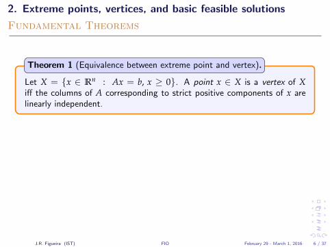
Let X = {x ∈ Rn : Ax = b, x ≥ 0}. A point x ∈ X is a vertex of Xiff the columns of A corresponding to strict positive components of x arelinearly independent.
Theorem 1 (Equivalence between extreme point and vertex).
J.R. Figueira (IST) FIO February 29 - March 1, 2016 6 / 37

2. Extreme points, vertices, and basic feasible solutions
Fundamental Theorems
Let X = {x ∈ Rn : Ax = b, x ≥ 0}. A point x ∈ X is a vertex of Xiff the columns of A corresponding to strict positive components of x arelinearly independent.
Theorem 1 (Equivalence between extreme point and vertex).
J.R. Figueira (IST) FIO February 29 - March 1, 2016 6 / 37
2. Extreme points, vertices, and basic feasible solutions
Definition of solution and feasible solution
Given a problem in a canonical form, a solution is a point that fulfills thefunctional constraints. If it also satisfies the nonnegativity constraints it iscalled a feasible solution, and in addition if it leads to the maximum of zit is called optimal solution.
Definition 1 (Solution, feasible solution, and optimal solution).
Let A denote an m× n (n > m) full row rank matrix. The characterization of a vertex
(geometric concept) requires to define a basic solution (algebraic concept).
Let B denote a non-singular m×m matrix composed of linear independentcolumns of A, called basis. The n−m components (variables) of x thatare not associated with B can be set equal to zero and they are callednonbasic variables. Then, the system Ax = b can be solved for the othercomponents (variables) of x, called basic variables. The resulting solutionof x is called basic solution. If the values are all nonnegative, it is called abasic feasible solution.
Definition 2 (Basic solution and basic feasible solution).
J.R. Figueira (IST) FIO February 29 - March 1, 2016 7 / 37
2. Extreme points, vertices, and basic feasible solutions
Extreme point, vertex, and basic feasible solution
A point x ∈ X is a vertex of X iff x is a basic feasible solution associatedwith some basis B.
Corollary 1 (Vertex and basic feasible solution).
A polyhedron X (as it was defined in this course) has a finite number ofvertices.
Corollary 2 (Number of vertices of a polyhedra).
J.R. Figueira (IST) FIO February 29 - March 1, 2016 8 / 37
3. The representation theorem
Representation theorem
A direction of a polyhedron X is a nonzero vector d ∈ Rn, such that forany point x0 ∈ X the ray {x ∈ Rn : x = x0 + λd, λ > 0} belongs to X.
Definition 3 (Direction of a polyhedron).
Let V = {v1, . . . , vk, . . . , vK} the set of vertices of X. Any point x ∈ Xcan be represented as
x =K
∑k=1
λkvk + d,K
∑k=1
λk = 1, λk > 0, k = 1, . . . , K,
and either d is a direction of X or d = 0 (in this case we are at a vertex).
Theorem 2 (Representation theorem).
If X is a polytope, then x ∈ X can be represented as a convex combinationof its vertices.
Corollary 3 (Polytope).
J.R. Figueira (IST) FIO February 29 - March 1, 2016 9 / 37
4. Fundamental theorems in LP
Two fundamental theorems in LP
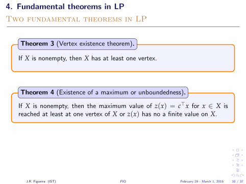
If X is nonempty, then X has at least one vertex.
Theorem 3 (Vertex existence theorem).
If X is nonempty, then the maximum value of z(x) = c>x for x ∈ X isreached at least at one vertex of X or z(x) has no a finite value on X.
Theorem 4 (Existence of a maximum or unboundedness).
J.R. Figueira (IST) FIO February 29 - March 1, 2016 10 / 37
4. Fundamental theorems in LP
Two fundamental theorems in LP
If X is nonempty, then X has at least one vertex.
Theorem 3 (Vertex existence theorem).
If X is nonempty, then the maximum value of z(x) = c>x for x ∈ X isreached at least at one vertex of X or z(x) has no a finite value on X.
Theorem 4 (Existence of a maximum or unboundedness).
J.R. Figueira (IST) FIO February 29 - March 1, 2016 10 / 37
5. The two variables LP example
The EERT-GIF Company: LP instance
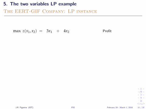
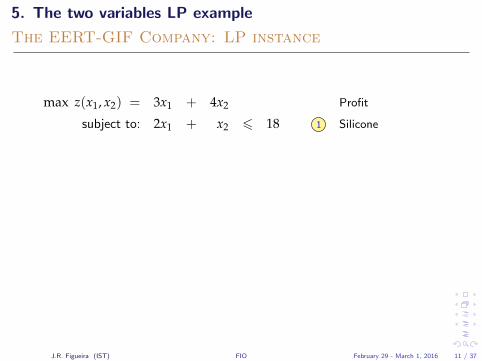
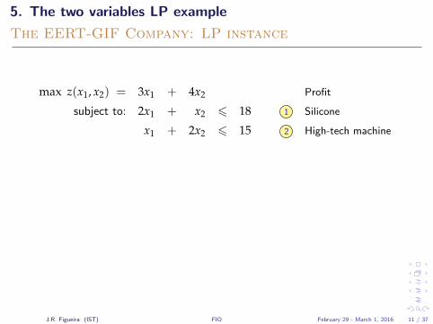
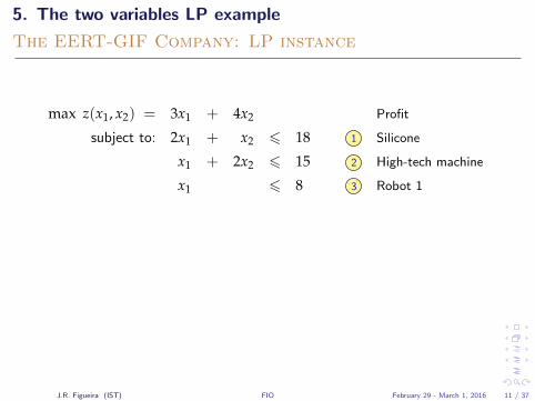
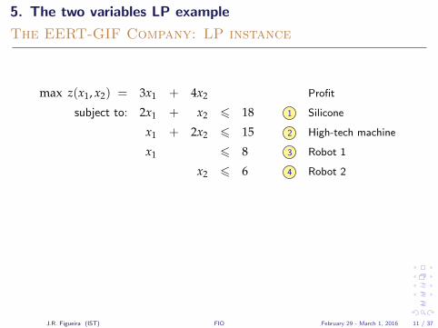
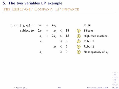
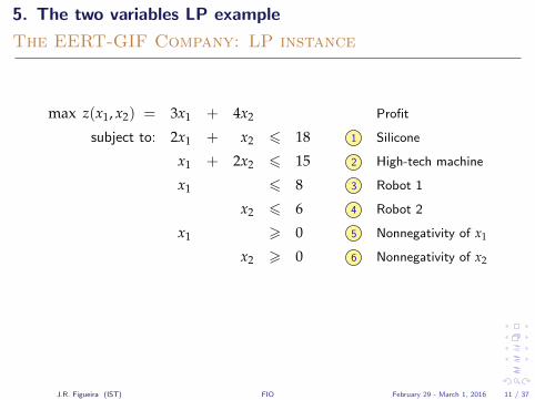
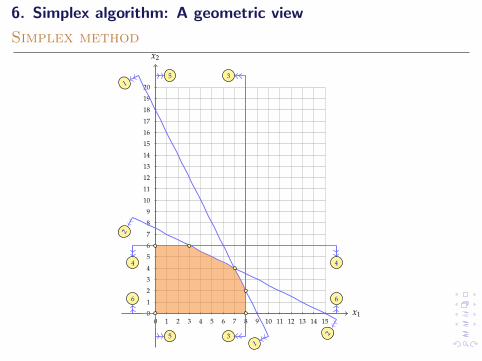
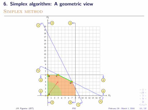
max z(x1, x2) = 3x1 + 4x2 Profit
subject to: 2x1 + x2 6 18 1 Silicone
x1 + 2x2 6 15 2 High-tech machine
x1 6 8 3 Robot 1
x2 6 6 4 Robot 2
x1 > 0 5 Nonnegativity of x1
x2 > 0 6 Nonnegativity of x2
J.R. Figueira (IST) FIO February 29 - March 1, 2016 11 / 37
5. The two variables LP example
The EERT-GIF Company: LP instance
max z(x1, x2) = 3x1 + 4x2 Profit
subject to: 2x1 + x2 6 18 1 Silicone
x1 + 2x2 6 15 2 High-tech machine
x1 6 8 3 Robot 1
x2 6 6 4 Robot 2
x1 > 0 5 Nonnegativity of x1
x2 > 0 6 Nonnegativity of x2
J.R. Figueira (IST) FIO February 29 - March 1, 2016 11 / 37
6. Simplex algorithm: A geometric view
Main idea and steps of Simplex method by G. Dantzig
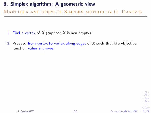
1. Find a vertex of X (suppose X is non-empty).
2. Proceed from vertex to vertex along edges of X such that the objectivefunction value improves.
3. Either the optimal vertex is reached, or an edge is selected which goes off toinfinity and along which the objective function value is unbounded.
J.R. Figueira (IST) FIO February 29 - March 1, 2016 12 / 37
6. Simplex algorithm: A geometric view
Main idea and steps of Simplex method by G. Dantzig
1. Find a vertex of X (suppose X is non-empty).
2. Proceed from vertex to vertex along edges of X such that the objectivefunction value improves.
3. Either the optimal vertex is reached, or an edge is selected which goes off toinfinity and along which the objective function value is unbounded.
J.R. Figueira (IST) FIO February 29 - March 1, 2016 12 / 37
6. Simplex algorithm: A geometric view
Simplex method
x1
x2
0 1 2 3 4 5 6 7 8 9 10 11 12 13 14 150
1
2
3
4
5
6
7
8
9
10
11
12
13
14
15
16
17
18
19
201
1
2
23
3
4 4
5
5
6 6A
B C
D
J.R. Figueira (IST) FIO February 29 - March 1, 2016 13 / 37
6. Simplex algorithm: A geometric view
Simplex method
x1
x2
0 1 2 3 4 5 6 7 8 9 10 11 12 13 14 150
1
2
3
4
5
6
7
8
9
10
11
12
13
14
15
16
17
18
19
201
1
2
23
3
4 4
5
5
6 6
A
B C
D
J.R. Figueira (IST) FIO February 29 - March 1, 2016 13 / 37

6. Simplex algorithm: A geometric view
Simplex method
x1
x2
0 1 2 3 4 5 6 7 8 9 10 11 12 13 14 150
1
2
3
4
5
6
7
8
9
10
11
12
13
14
15
16
17
18
19
201
1
2
23
3
4 4
5
5
6 6
A
B C
D
J.R. Figueira (IST) FIO February 29 - March 1, 2016 13 / 37

6. Simplex algorithm: A geometric view
Simplex method
x1
x2
0 1 2 3 4 5 6 7 8 9 10 11 12 13 14 150
1
2
3
4
5
6
7
8
9
10
11
12
13
14
15
16
17
18
19
201
1
2
23
3
4 4
5
5
6 6
A
B C
D
J.R. Figueira (IST) FIO February 29 - March 1, 2016 13 / 37

6. Simplex algorithm: A geometric view
Simplex method
x1
x2
0 1 2 3 4 5 6 7 8 9 10 11 12 13 14 150
1
2
3
4
5
6
7
8
9
10
11
12
13
14
15
16
17
18
19
201
1
2
23
3
4 4
5
5
6 6A
B C
D
J.R. Figueira (IST) FIO February 29 - March 1, 2016 13 / 37

6. Simplex algorithm: A geometric view
Simplex method
x1
x2
0 1 2 3 4 5 6 7 8 9 10 11 12 13 14 150
1
2
3
4
5
6
7
8
9
10
11
12
13
14
15
16
17
18
19
201
1
2
23
3
4 4
5
5
6 6A
B
C
D
J.R. Figueira (IST) FIO February 29 - March 1, 2016 13 / 37

6. Simplex algorithm: A geometric view
Simplex method
x1
x2
0 1 2 3 4 5 6 7 8 9 10 11 12 13 14 150
1
2
3
4
5
6
7
8
9
10
11
12
13
14
15
16
17
18
19
201
1
2
23
3
4 4
5
5
6 6A
B C
D
J.R. Figueira (IST) FIO February 29 - March 1, 2016 13 / 37

6. Simplex algorithm: A geometric view
Simplex method
x1
x2
0 1 2 3 4 5 6 7 8 9 10 11 12 13 14 150
1
2
3
4
5
6
7
8
9
10
11
12
13
14
15
16
17
18
19
201
1
2
23
3
4 4
5
5
6 6A
B C
D
J.R. Figueira (IST) FIO February 29 - March 1, 2016 13 / 37
6. Simplex algorithm: A geometric view
Simplex method
x1
x2
0 1 2 3 4 5 6 7 8 9 10 11 12 13 14 150
1
2
3
4
5
6
7
8
9
10
11
12
13
14
15
16
17
18
19
201
1
2
23
3
4 4
5
5
6 6A
B C
D
J.R. Figueira (IST) FIO February 29 - March 1, 2016 13 / 37
Part
Simplex Algorithm

Contents
1. Introduction
2. An appropriate LP form
3. A dictionary
4. The simplex in an algebraic form
5. Tabular form of simplex: Introduction
6. Tabular form: Results and interpretation
Contents
1. Introduction
2. An appropriate LP form
3. A dictionary
4. The simplex in an algebraic form
5. Tabular form of simplex: Introduction
6. Tabular form: Results and interpretation
Contents
1. Introduction
2. An appropriate LP form
3. A dictionary
4. The simplex in an algebraic form
5. Tabular form of simplex: Introduction
6. Tabular form: Results and interpretation
Contents
1. Introduction
2. An appropriate LP form
3. A dictionary
4. The simplex in an algebraic form
5. Tabular form of simplex: Introduction
6. Tabular form: Results and interpretation
Contents
1. Introduction
2. An appropriate LP form
3. A dictionary
4. The simplex in an algebraic form
5. Tabular form of simplex: Introduction
6. Tabular form: Results and interpretation
Contents
1. Introduction
2. An appropriate LP form
3. A dictionary
4. The simplex in an algebraic form
5. Tabular form of simplex: Introduction
6. Tabular form: Results and interpretation
1. Introduction
Introduction
I Find an appropriated form of the LP.
I Some more concepts needed.
I An algebraic version of simplex method.
I The basis for a tabular version.
I More on the tabular version and how to interpret the results.
J.R. Figueira (IST) FIO February 29 - March 1, 2016 16 / 37
1. Introduction
Introduction
I Find an appropriated form of the LP.
I Some more concepts needed.
I An algebraic version of simplex method.
I The basis for a tabular version.
I More on the tabular version and how to interpret the results.
J.R. Figueira (IST) FIO February 29 - March 1, 2016 16 / 37
1. Introduction
Introduction
I Find an appropriated form of the LP.
I Some more concepts needed.
I An algebraic version of simplex method.
I The basis for a tabular version.
I More on the tabular version and how to interpret the results.
J.R. Figueira (IST) FIO February 29 - March 1, 2016 16 / 37
1. Introduction
Introduction
I Find an appropriated form of the LP.
I Some more concepts needed.
I An algebraic version of simplex method.
I The basis for a tabular version.
I More on the tabular version and how to interpret the results.
J.R. Figueira (IST) FIO February 29 - March 1, 2016 16 / 37
1. Introduction
Introduction
I Find an appropriated form of the LP.
I Some more concepts needed.
I An algebraic version of simplex method.
I The basis for a tabular version.
I More on the tabular version and how to interpret the results.
J.R. Figueira (IST) FIO February 29 - March 1, 2016 16 / 37
1. Introduction
Introduction
I Find an appropriated form of the LP.
I Some more concepts needed.
I An algebraic version of simplex method.
I The basis for a tabular version.
I More on the tabular version and how to interpret the results.
J.R. Figueira (IST) FIO February 29 - March 1, 2016 16 / 37
2. An appropriate LP form
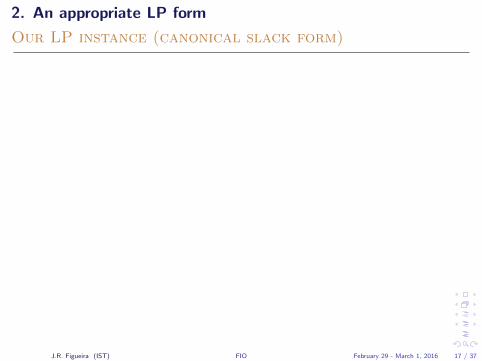
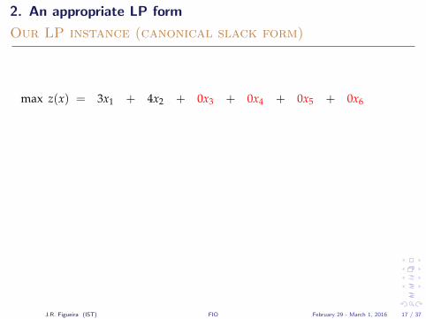
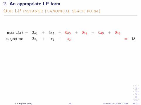
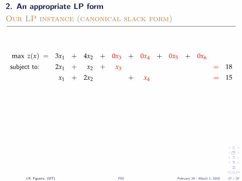
Our LP instance (canonical slack form)
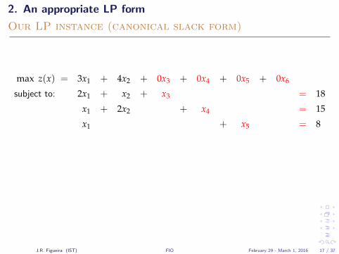
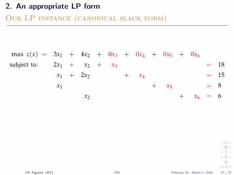
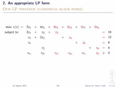
max z(x) = 3x1 + 4x2 + 0x3 + 0x4 + 0x5 + 0x6
subject to: 2x1 + x2 + x3 = 18
x1 + 2x2 + x4 = 15
x1 + x5 = 8
x2 + x6 = 6
x1, x2, x3, x4, x5, x6 > 0
J.R. Figueira (IST) FIO February 29 - March 1, 2016 17 / 37
2. An appropriate LP form
Our LP instance (canonical slack form)
max z(x) = 3x1 + 4x2 + 0x3 + 0x4 + 0x5 + 0x6
subject to: 2x1 + x2 + x3 = 18
x1 + 2x2 + x4 = 15
x1 + x5 = 8
x2 + x6 = 6
x1, x2, x3, x4, x5, x6 > 0
J.R. Figueira (IST) FIO February 29 - March 1, 2016 17 / 37
2. An appropriate LP form
Our LP instance (canonical slack form)
max z(x) = 3x1 + 4x2 + 0x3 + 0x4 + 0x5 + 0x6
subject to: 2x1 + x2 + x3 = 18
x1 + 2x2 + x4 = 15
x1 + x5 = 8
x2 + x6 = 6
x1, x2, x3, x4, x5, x6 > 0
J.R. Figueira (IST) FIO February 29 - March 1, 2016 17 / 37
2. An appropriate LP form
Our LP instance (canonical slack form)
max z(x) = 3x1 + 4x2 + 0x3 + 0x4 + 0x5 + 0x6
subject to: 2x1 + x2 + x3 = 18
x1 + 2x2 + x4 = 15
x1 + x5 = 8
x2 + x6 = 6
x1, x2, x3, x4, x5, x6 > 0
J.R. Figueira (IST) FIO February 29 - March 1, 2016 17 / 37
2. An appropriate LP form
Our LP instance (canonical slack form)
max z(x) = 3x1 + 4x2 + 0x3 + 0x4 + 0x5 + 0x6
subject to: 2x1 + x2 + x3 = 18
x1 + 2x2 + x4 = 15
x1 + x5 = 8
x2 + x6 = 6
x1, x2, x3, x4, x5, x6 > 0
J.R. Figueira (IST) FIO February 29 - March 1, 2016 17 / 37
2. An appropriate LP form
Our LP instance (canonical slack form)
max z(x) = 3x1 + 4x2 + 0x3 + 0x4 + 0x5 + 0x6
subject to: 2x1 + x2 + x3 = 18
x1 + 2x2 + x4 = 15
x1 + x5 = 8
x2 + x6 = 6
x1, x2, x3, x4, x5, x6 > 0
J.R. Figueira (IST) FIO February 29 - March 1, 2016 17 / 37

2. An appropriate LP form
Our LP instance (canonical slack form)
max z(x) = 3x1 + 4x2 + 0x3 + 0x4 + 0x5 + 0x6
subject to: 2x1 + x2 + x3 = 18
x1 + 2x2 + x4 = 15
x1 + x5 = 8
x2 + x6 = 6
x1, x2, x3, x4, x5, x6 > 0
J.R. Figueira (IST) FIO February 29 - March 1, 2016 17 / 37
2. An appropriate LP form
Our LP instance (canonical slack form)
max z(x) = 3x1 + 4x2 + 0x3 + 0x4 + 0x5 + 0x6
subject to: 2x1 + x2 + x3 = 18
x1 + 2x2 + x4 = 15
x1 + x5 = 8
x2 + x6 = 6
x1, x2, x3, x4, x5, x6 > 0
J.R. Figueira (IST) FIO February 29 - March 1, 2016 17 / 37
2. An appropriate LP form
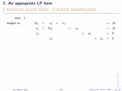
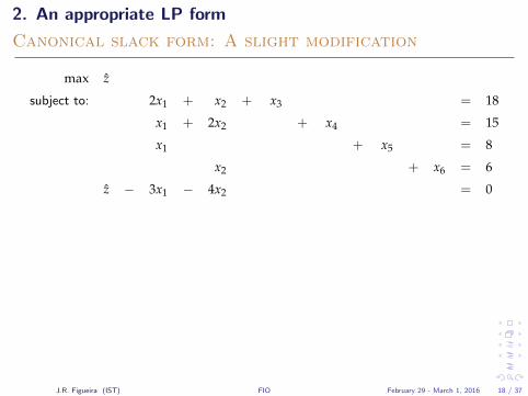
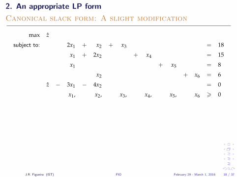
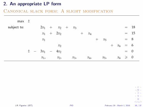
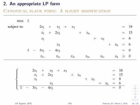
Canonical slack form: A slight modification
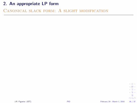
max z
subject to: 2x1 + x2 + x3 = 18
x1 + 2x2 + x4 = 15
x1 + x5 = 8
x2 + x6 = 6
z − 3x1 − 4x2 = 0
x1, x2, x3, x4, x5, x6 > 0
2x1 + x2 + x3 = 18x1 + 2x2 + x4 = 15x1 + x5 = 8
x2 + x6 = 6z − 3x1 − 4x2 = 0
J.R. Figueira (IST) FIO February 29 - March 1, 2016 18 / 37
2. An appropriate LP form
Canonical slack form: A slight modification
max z
subject to: 2x1 + x2 + x3 = 18
x1 + 2x2 + x4 = 15
x1 + x5 = 8
x2 + x6 = 6
z − 3x1 − 4x2 = 0
x1, x2, x3, x4, x5, x6 > 0
2x1 + x2 + x3 = 18x1 + 2x2 + x4 = 15x1 + x5 = 8
x2 + x6 = 6z − 3x1 − 4x2 = 0
J.R. Figueira (IST) FIO February 29 - March 1, 2016 18 / 37
2. An appropriate LP form
Canonical slack form: A slight modification
max z
subject to: 2x1 + x2 + x3 = 18
x1 + 2x2 + x4 = 15
x1 + x5 = 8
x2 + x6 = 6
z − 3x1 − 4x2 = 0
x1, x2, x3, x4, x5, x6 > 0
2x1 + x2 + x3 = 18
x1 + 2x2 + x4 = 15x1 + x5 = 8
x2 + x6 = 6z − 3x1 − 4x2 = 0
J.R. Figueira (IST) FIO February 29 - March 1, 2016 18 / 37
3. A dictionary
Dictionaries
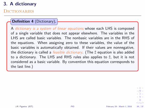
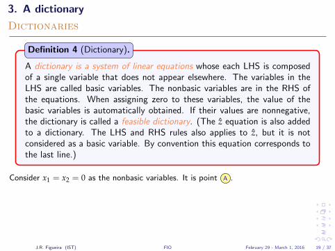
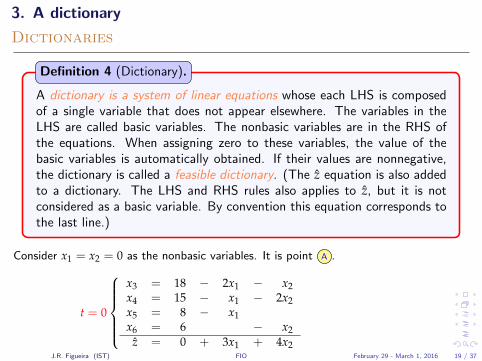
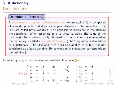
A dictionary is a system of linear equations whose each LHS is composedof a single variable that does not appear elsewhere. The variables in theLHS are called basic variables. The nonbasic variables are in the RHS ofthe equations. When assigning zero to these variables, the value of thebasic variables is automatically obtained. If their values are nonnegative,the dictionary is called a feasible dictionary. (The z equation is also addedto a dictionary. The LHS and RHS rules also applies to z, but it is notconsidered as a basic variable. By convention this equation corresponds tothe last line.)
Definition 4 (Dictionary).
Consider x1 = x2 = 0 as the nonbasic variables. It is point A .
t = 0
x3 = 18 − 2x1 − x2x4 = 15 − x1 − 2x2x5 = 8 − x1x6 = 6 − x2
z = 0 + 3x1 + 4x2
x3 = 18x4 = 15x5 = 8x6 = 6
z = 0
J.R. Figueira (IST) FIO February 29 - March 1, 2016 19 / 37
3. A dictionary
Dictionaries
A dictionary is a system of linear equations whose each LHS is composedof a single variable that does not appear elsewhere. The variables in theLHS are called basic variables. The nonbasic variables are in the RHS ofthe equations. When assigning zero to these variables, the value of thebasic variables is automatically obtained. If their values are nonnegative,the dictionary is called a feasible dictionary. (The z equation is also addedto a dictionary. The LHS and RHS rules also applies to z, but it is notconsidered as a basic variable. By convention this equation corresponds tothe last line.)
Definition 4 (Dictionary).
Consider x1 = x2 = 0 as the nonbasic variables. It is point A .
t = 0
x3 = 18 − 2x1 − x2x4 = 15 − x1 − 2x2x5 = 8 − x1x6 = 6 − x2
z = 0 + 3x1 + 4x2
x3 = 18x4 = 15x5 = 8x6 = 6
z = 0J.R. Figueira (IST) FIO February 29 - March 1, 2016 19 / 37
4. The simplex in an algebraic form
Moving to another basic feasible solution
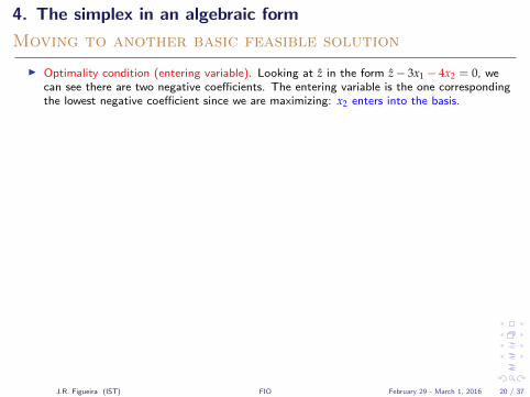
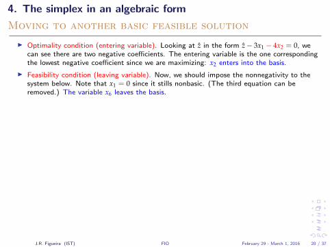
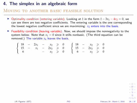
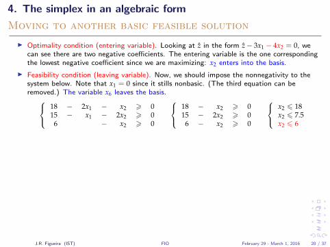
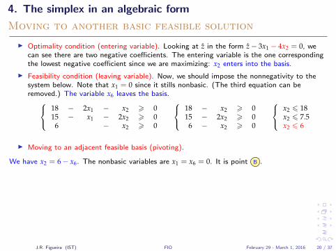
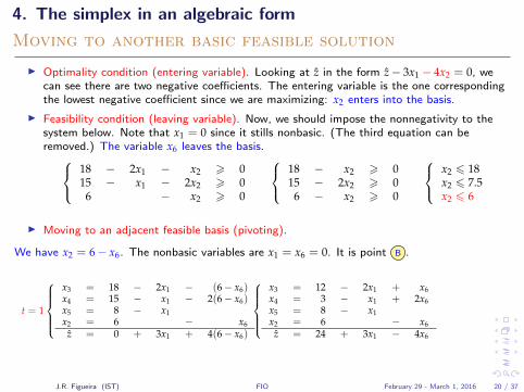
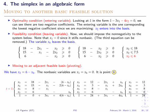
I Optimality condition (entering variable). Looking at z in the form z− 3x1 − 4x2 = 0, wecan see there are two negative coefficients. The entering variable is the one correspondingthe lowest negative coefficient since we are maximizing: x2 enters into the basis.
I Feasibility condition (leaving variable). Now, we should impose the nonnegativity to thesystem below. Note that x1 = 0 since it stills nonbasic. (The third equation can beremoved.) The variable x6 leaves the basis. 18 − 2x1 − x2 > 0
15 − x1 − 2x2 > 06 − x2 > 0
18 − x2 > 015 − 2x2 > 0
6 − x2 > 0
x2 6 18x2 6 7.5x2 6 6
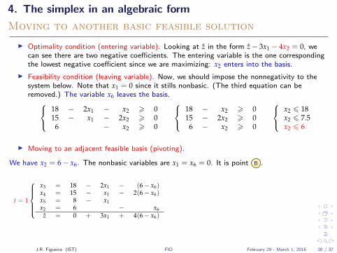
I Moving to an adjacent feasible basis (pivoting).
We have x2 = 6− x6. The nonbasic variables are x1 = x6 = 0. It is point B .
t = 1
x3 = 18 − 2x1 − (6− x6)x4 = 15 − x1 − 2(6− x6)x5 = 8 − x1x2 = 6 − x6z = 0 + 3x1 + 4(6− x6)
x3 = 12 − 2x1 + x6x4 = 3 − x1 + 2x6x5 = 8 − x1x2 = 6 − x6z = 24 + 3x1 − 4x6
x3 = 12x4 = 3x5 = 8x2 = 6z = 24
J.R. Figueira (IST) FIO February 29 - March 1, 2016 20 / 37
4. The simplex in an algebraic form
Moving to another basic feasible solution
I Optimality condition (entering variable). Looking at z in the form z− 3x1 − 4x2 = 0, wecan see there are two negative coefficients. The entering variable is the one correspondingthe lowest negative coefficient since we are maximizing: x2 enters into the basis.
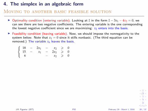
I Feasibility condition (leaving variable). Now, we should impose the nonnegativity to thesystem below. Note that x1 = 0 since it stills nonbasic. (The third equation can beremoved.) The variable x6 leaves the basis.
18 − 2x1 − x2 > 015 − x1 − 2x2 > 0
6 − x2 > 0
18 − x2 > 015 − 2x2 > 0
6 − x2 > 0
x2 6 18x2 6 7.5x2 6 6
I Moving to an adjacent feasible basis (pivoting).
We have x2 = 6− x6. The nonbasic variables are x1 = x6 = 0. It is point B .
t = 1
x3 = 18 − 2x1 − (6− x6)x4 = 15 − x1 − 2(6− x6)x5 = 8 − x1x2 = 6 − x6z = 0 + 3x1 + 4(6− x6)
x3 = 12 − 2x1 + x6x4 = 3 − x1 + 2x6x5 = 8 − x1x2 = 6 − x6z = 24 + 3x1 − 4x6
x3 = 12x4 = 3x5 = 8x2 = 6z = 24
J.R. Figueira (IST) FIO February 29 - March 1, 2016 20 / 37
4. The simplex in an algebraic form
Moving to another basic feasible solution
I Optimality condition (entering variable). Looking at z in the form z− 3x1 − 4x2 = 0, wecan see there are two negative coefficients. The entering variable is the one correspondingthe lowest negative coefficient since we are maximizing: x2 enters into the basis.
I Feasibility condition (leaving variable). Now, we should impose the nonnegativity to thesystem below. Note that x1 = 0 since it stills nonbasic. (The third equation can beremoved.) The variable x6 leaves the basis. 18 − 2x1 − x2 > 0
15 − x1 − 2x2 > 06 − x2 > 0
18 − x2 > 015 − 2x2 > 0
6 − x2 > 0
x2 6 18x2 6 7.5x2 6 6
I Moving to an adjacent feasible basis (pivoting).
We have x2 = 6− x6. The nonbasic variables are x1 = x6 = 0. It is point B .
t = 1
x3 = 18 − 2x1 − (6− x6)x4 = 15 − x1 − 2(6− x6)x5 = 8 − x1x2 = 6 − x6z = 0 + 3x1 + 4(6− x6)
x3 = 12 − 2x1 + x6x4 = 3 − x1 + 2x6x5 = 8 − x1x2 = 6 − x6z = 24 + 3x1 − 4x6
x3 = 12x4 = 3x5 = 8x2 = 6z = 24
J.R. Figueira (IST) FIO February 29 - March 1, 2016 20 / 37
4. The simplex in an algebraic form
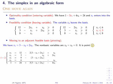
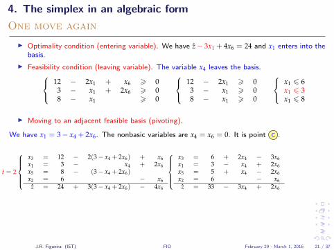
One move again
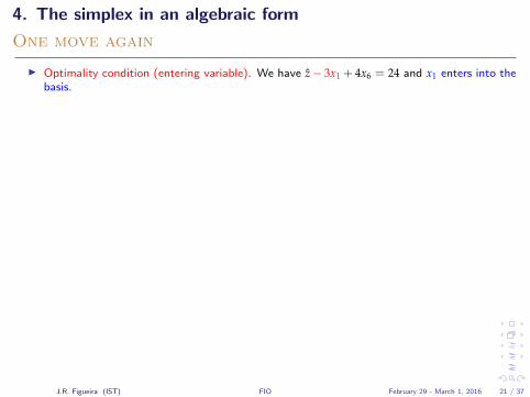
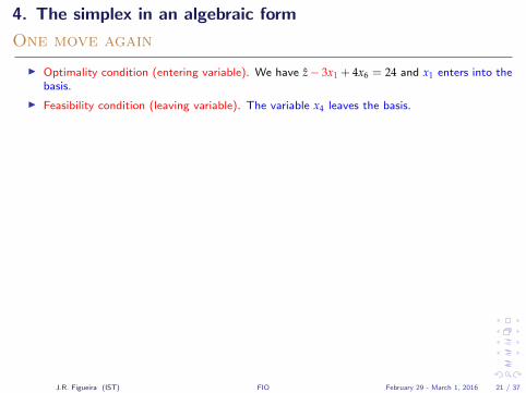
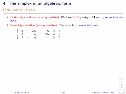
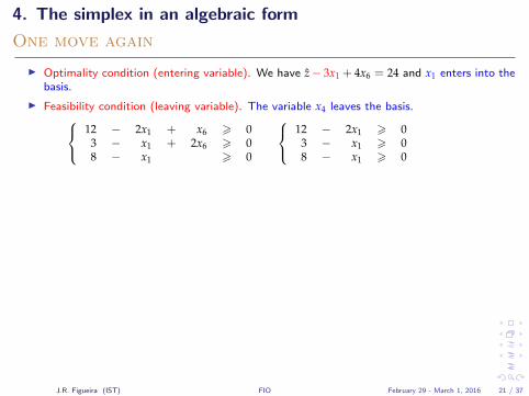
I Optimality condition (entering variable). We have z− 3x1 + 4x6 = 24 and x1 enters into thebasis.
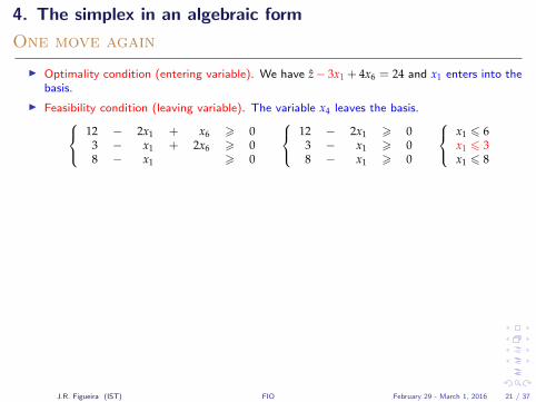
I Feasibility condition (leaving variable). The variable x4 leaves the basis. 12 − 2x1 + x6 > 03 − x1 + 2x6 > 08 − x1 > 0
12 − 2x1 > 03 − x1 > 08 − x1 > 0
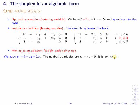
x1 6 6x1 6 3x1 6 8
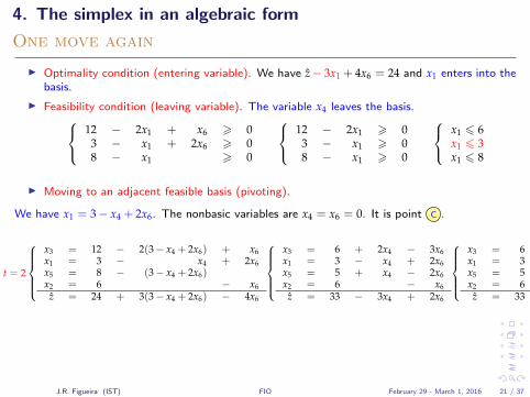
I Moving to an adjacent feasible basis (pivoting).
We have x1 = 3− x4 + 2x6. The nonbasic variables are x4 = x6 = 0. It is point C .
t = 2
x3 = 12 − 2(3− x4 + 2x6) + x6x1 = 3 − x4 + 2x6x5 = 8 − (3− x4 + 2x6)x2 = 6 − x6z = 24 + 3(3− x4 + 2x6) − 4x6
x3 = 6 + 2x4 − 3x6x1 = 3 − x4 + 2x6x5 = 5 + x4 − 2x6x2 = 6 − x6z = 33 − 3x4 + 2x6
x3 = 6x1 = 3x5 = 5x2 = 6z = 33
J.R. Figueira (IST) FIO February 29 - March 1, 2016 21 / 37
4. The simplex in an algebraic form
One move again
I Optimality condition (entering variable). We have z− 3x1 + 4x6 = 24 and x1 enters into thebasis.
I Feasibility condition (leaving variable). The variable x4 leaves the basis.
12 − 2x1 + x6 > 03 − x1 + 2x6 > 08 − x1 > 0
12 − 2x1 > 03 − x1 > 08 − x1 > 0
x1 6 6x1 6 3x1 6 8
I Moving to an adjacent feasible basis (pivoting).
We have x1 = 3− x4 + 2x6. The nonbasic variables are x4 = x6 = 0. It is point C .
t = 2
x3 = 12 − 2(3− x4 + 2x6) + x6x1 = 3 − x4 + 2x6x5 = 8 − (3− x4 + 2x6)x2 = 6 − x6z = 24 + 3(3− x4 + 2x6) − 4x6
x3 = 6 + 2x4 − 3x6x1 = 3 − x4 + 2x6x5 = 5 + x4 − 2x6x2 = 6 − x6z = 33 − 3x4 + 2x6
x3 = 6x1 = 3x5 = 5x2 = 6z = 33
J.R. Figueira (IST) FIO February 29 - March 1, 2016 21 / 37
4. The simplex in an algebraic form
One move again
I Optimality condition (entering variable). We have z− 3x1 + 4x6 = 24 and x1 enters into thebasis.
I Feasibility condition (leaving variable). The variable x4 leaves the basis. 12 − 2x1 + x6 > 03 − x1 + 2x6 > 08 − x1 > 0
12 − 2x1 > 03 − x1 > 08 − x1 > 0
x1 6 6x1 6 3x1 6 8
I Moving to an adjacent feasible basis (pivoting).
We have x1 = 3− x4 + 2x6. The nonbasic variables are x4 = x6 = 0. It is point C .
t = 2
x3 = 12 − 2(3− x4 + 2x6) + x6x1 = 3 − x4 + 2x6x5 = 8 − (3− x4 + 2x6)x2 = 6 − x6z = 24 + 3(3− x4 + 2x6) − 4x6
x3 = 6 + 2x4 − 3x6x1 = 3 − x4 + 2x6x5 = 5 + x4 − 2x6x2 = 6 − x6z = 33 − 3x4 + 2x6
x3 = 6x1 = 3x5 = 5x2 = 6z = 33
J.R. Figueira (IST) FIO February 29 - March 1, 2016 21 / 37
4. The simplex in an algebraic form
The last move
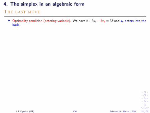
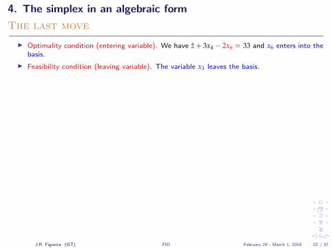
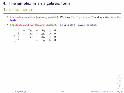
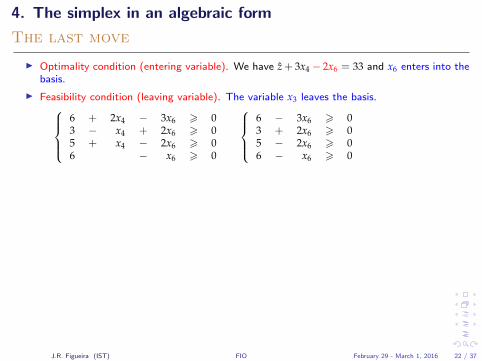
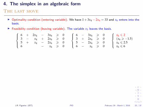
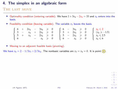
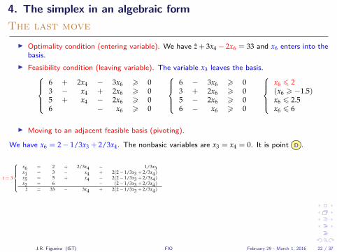
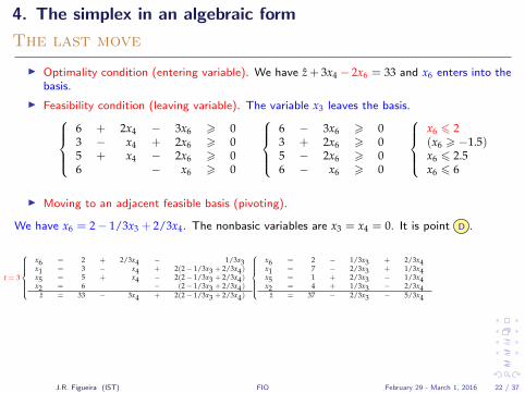
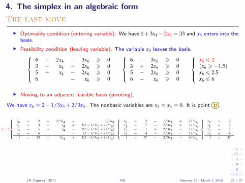
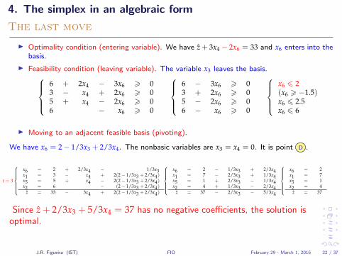
I Optimality condition (entering variable). We have z + 3x4 − 2x6 = 33 and x6 enters into thebasis.
I Feasibility condition (leaving variable). The variable x3 leaves the basis.6 + 2x4 − 3x6 > 03 − x4 + 2x6 > 05 + x4 − 2x6 > 06 − x6 > 0
6 − 3x6 > 03 + 2x6 > 05 − 2x6 > 06 − x6 > 0
x6 6 2(x6 > −1.5)x6 6 2.5x6 6 6
I Moving to an adjacent feasible basis (pivoting).
We have x6 = 2− 1/3x3 + 2/3x4. The nonbasic variables are x3 = x4 = 0. It is point D .
t = 3
x6 = 2 + 2/3x4 − 1/3x3x1 = 3 − x4 + 2(2− 1/3x3 + 2/3x4)x5 = 5 + x4 − 2(2− 1/3x3 + 2/3x4)x2 = 6 − (2− 1/3x3 + 2/3x4)
z = 33 − 3x4 + 2(2− 1/3x3 + 2/3x4)
x6 = 2 − 1/3x3 + 2/3x4x1 = 7 − 2/3x3 + 1/3x4x5 = 1 + 2/3x3 − 1/3x4x2 = 4 + 1/3x3 − 2/3x4
z = 37 − 2/3x3 − 5/3x4
x6 = 2x1 = 7x5 = 1x2 = 4
z = 37
Since z + 2/3x3 + 5/3x4 = 37 has no negative coefficients, the solution isoptimal.
J.R. Figueira (IST) FIO February 29 - March 1, 2016 22 / 37
4. The simplex in an algebraic form
The last move
I Optimality condition (entering variable). We have z + 3x4 − 2x6 = 33 and x6 enters into thebasis.
I Feasibility condition (leaving variable). The variable x3 leaves the basis.
6 + 2x4 − 3x6 > 03 − x4 + 2x6 > 05 + x4 − 2x6 > 06 − x6 > 0
6 − 3x6 > 03 + 2x6 > 05 − 2x6 > 06 − x6 > 0
x6 6 2(x6 > −1.5)x6 6 2.5x6 6 6
I Moving to an adjacent feasible basis (pivoting).
We have x6 = 2− 1/3x3 + 2/3x4. The nonbasic variables are x3 = x4 = 0. It is point D .
t = 3
x6 = 2 + 2/3x4 − 1/3x3x1 = 3 − x4 + 2(2− 1/3x3 + 2/3x4)x5 = 5 + x4 − 2(2− 1/3x3 + 2/3x4)x2 = 6 − (2− 1/3x3 + 2/3x4)
z = 33 − 3x4 + 2(2− 1/3x3 + 2/3x4)
x6 = 2 − 1/3x3 + 2/3x4x1 = 7 − 2/3x3 + 1/3x4x5 = 1 + 2/3x3 − 1/3x4x2 = 4 + 1/3x3 − 2/3x4
z = 37 − 2/3x3 − 5/3x4
x6 = 2x1 = 7x5 = 1x2 = 4
z = 37
Since z + 2/3x3 + 5/3x4 = 37 has no negative coefficients, the solution isoptimal.
J.R. Figueira (IST) FIO February 29 - March 1, 2016 22 / 37
4. The simplex in an algebraic form
The last move
I Optimality condition (entering variable). We have z + 3x4 − 2x6 = 33 and x6 enters into thebasis.
I Feasibility condition (leaving variable). The variable x3 leaves the basis.6 + 2x4 − 3x6 > 03 − x4 + 2x6 > 05 + x4 − 2x6 > 06 − x6 > 0
6 − 3x6 > 03 + 2x6 > 05 − 2x6 > 06 − x6 > 0
x6 6 2(x6 > −1.5)x6 6 2.5x6 6 6
I Moving to an adjacent feasible basis (pivoting).
We have x6 = 2− 1/3x3 + 2/3x4. The nonbasic variables are x3 = x4 = 0. It is point D .
t = 3
x6 = 2 + 2/3x4 − 1/3x3x1 = 3 − x4 + 2(2− 1/3x3 + 2/3x4)x5 = 5 + x4 − 2(2− 1/3x3 + 2/3x4)x2 = 6 − (2− 1/3x3 + 2/3x4)
z = 33 − 3x4 + 2(2− 1/3x3 + 2/3x4)
x6 = 2 − 1/3x3 + 2/3x4x1 = 7 − 2/3x3 + 1/3x4x5 = 1 + 2/3x3 − 1/3x4x2 = 4 + 1/3x3 − 2/3x4
z = 37 − 2/3x3 − 5/3x4
x6 = 2x1 = 7x5 = 1x2 = 4
z = 37
Since z + 2/3x3 + 5/3x4 = 37 has no negative coefficients, the solution isoptimal.
J.R. Figueira (IST) FIO February 29 - March 1, 2016 22 / 37
4. The simplex in an algebraic form
The last move
I Optimality condition (entering variable). We have z + 3x4 − 2x6 = 33 and x6 enters into thebasis.
I Feasibility condition (leaving variable). The variable x3 leaves the basis.6 + 2x4 − 3x6 > 03 − x4 + 2x6 > 05 + x4 − 2x6 > 06 − x6 > 0
6 − 3x6 > 03 + 2x6 > 05 − 2x6 > 06 − x6 > 0
x6 6 2(x6 > −1.5)x6 6 2.5x6 6 6
I Moving to an adjacent feasible basis (pivoting).
We have x6 = 2− 1/3x3 + 2/3x4. The nonbasic variables are x3 = x4 = 0. It is point D .
t = 3
x6 = 2 + 2/3x4 − 1/3x3x1 = 3 − x4 + 2(2− 1/3x3 + 2/3x4)x5 = 5 + x4 − 2(2− 1/3x3 + 2/3x4)x2 = 6 − (2− 1/3x3 + 2/3x4)
z = 33 − 3x4 + 2(2− 1/3x3 + 2/3x4)
x6 = 2 − 1/3x3 + 2/3x4x1 = 7 − 2/3x3 + 1/3x4x5 = 1 + 2/3x3 − 1/3x4x2 = 4 + 1/3x3 − 2/3x4
z = 37 − 2/3x3 − 5/3x4
x6 = 2x1 = 7x5 = 1x2 = 4
z = 37
Since z + 2/3x3 + 5/3x4 = 37 has no negative coefficients, the solution isoptimal.
J.R. Figueira (IST) FIO February 29 - March 1, 2016 22 / 37
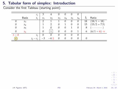
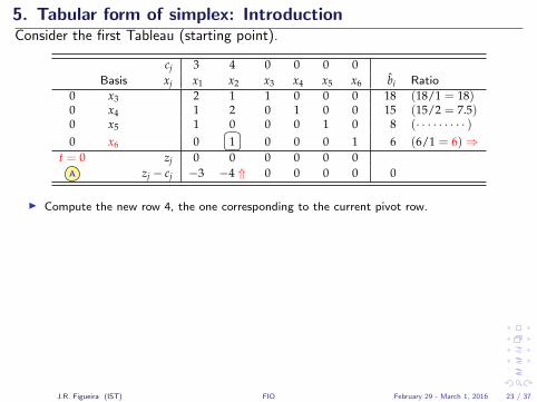
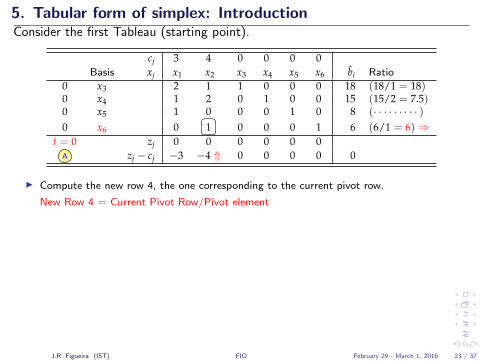
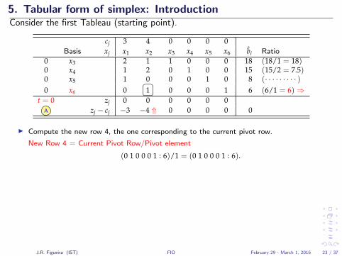
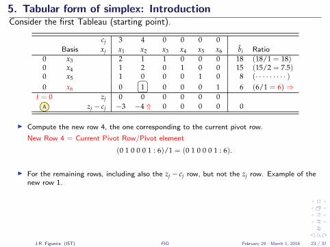
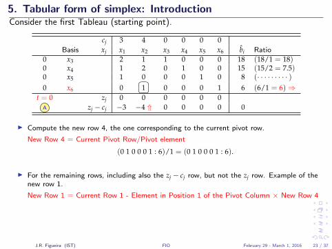
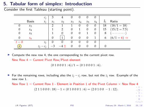
5. Tabular form of simplex: IntroductionConsider the first Tableau (starting point).
cj 3 4 0 0 0 0Basis xj x1 x2 x3 x4 x5 x6 bi Ratio
0 x3 2 1 1 0 0 0 18 (18/1 = 18)0 x4 1 2 0 1 0 0 15 (15/2 = 7.5)0 x5 1 0 0 0 1 0 8 (· · · · · · · · · )0 x6 0
�� ��1 0 0 0 1 6 (6/1 = 6)⇒t = 0 zj 0 0 0 0 0 0
A zj − cj −3 −4 ⇑ 0 0 0 0 0
I Compute the new row 4, the one corresponding to the current pivot row.
New Row 4 = Current Pivot Row/Pivot element
(0 1 0 0 0 1 : 6)/1 = (0 1 0 0 0 1 : 6).
I For the remaining rows, including also the zj − cj row, but not the zj row. Example of thenew row 1.
New Row 1 = Current Row 1 - Element in Position 1 of the Pivot Column × New Row 4
(2 1 1 0 0 0 : 18)− 1× (0 1 0 0 0 1 : 6) = (2 0 1 0 0 − 1 : 12).
I Do the same for the remaining rows.
J.R. Figueira (IST) FIO February 29 - March 1, 2016 23 / 37
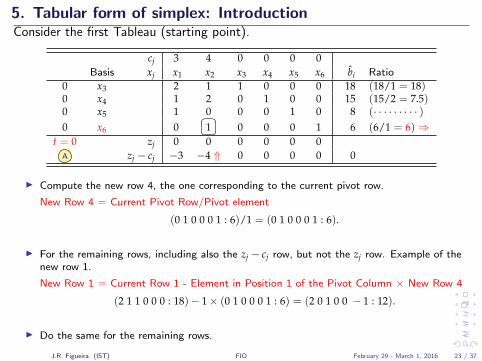
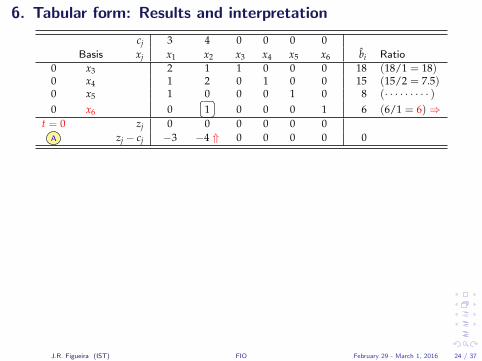
6. Tabular form: Results and interpretation
cj 3 4 0 0 0 0Basis xj x1 x2 x3 x4 x5 x6 bi Ratio
0 x3 2 1 1 0 0 0 18 (18/1 = 18)0 x4 1 2 0 1 0 0 15 (15/2 = 7.5)0 x5 1 0 0 0 1 0 8 (· · · · · · · · · )0 x6 0
�� ��1 0 0 0 1 6 (6/1 = 6)⇒t = 0 zj 0 0 0 0 0 0
A zj − cj −3 −4 ⇑ 0 0 0 0 0
0 x3 2 0 1 0 0 −1 12 (12/2 = 6)0 x4
�� ��1 0 0 1 0 −2 3 (3/1 = 3)⇒0 x5 1 0 0 0 1 0 8 (8/1 = 8)4 x2 0 1 0 0 0 1 6 (· · · · · · · · · )
t = 1 zj 0 4 0 0 0 4B zj − cj −3 ⇑ 0 0 0 0 4 24
0 x3 0 0 1 −2 0�� ��3 6 (6/3 = 2)⇒
3 x1 1 0 0 1 0 −2 3 (· · · · · · · · · )0 x5 0 0 0 −1 1 2 5 (5/2 = 2.5)4 x2 0 1 0 0 0 1 6 (6/1 = 6)
t = 2 zj 3 4 0 3 0 −2C zj − cj 0 0 0 3 0 −2 ⇑ 33
J.R. Figueira (IST) FIO February 29 - March 1, 2016 24 / 37
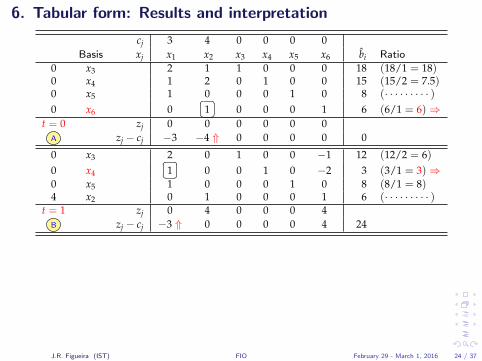
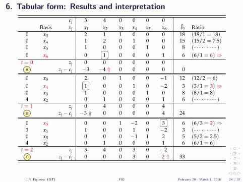
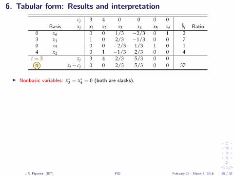
6. Tabular form: Results and interpretation
cj 3 4 0 0 0 0Basis xj x1 x2 x3 x4 x5 x6 bi Ratio
0 x6 0 0 1/3 −2/3 0 1 23 x1 1 0 2/3 −1/3 0 0 70 x5 0 0 −2/3 1/3 1 0 14 x2 0 1 −1/3 2/3 0 0 4
t = 3 zj 3 4 2/3 5/3 0 0D zj − cj 0 0 2/3 5/3 0 0 37
I Nonbasic variables: x∗3 = x∗4 = 0 (both are slacks).
x∗3 is associated with Silicone availability. Since x∗3 = 0, it means that all the Siliconewas used in the production.
x∗4 is associated with the High-Tech machine. Since x∗4 = 0, it means that we spend allthe time we could do in the High-Tech machine for our production.
I Basic variables: x∗1 = 7 means that the daily production of breast implants is 7 and x∗2 = 4means that we produce 4 facial implants. The daily profit is z∗ = 37 Euros.
x∗5 is associated with Robot 1. Since x∗5 = 1, it means that did not use Robot 1 in itsoverall availability. We have one hour left.
The interpretation of x∗6 is similar.
J.R. Figueira (IST) FIO February 29 - March 1, 2016 25 / 37
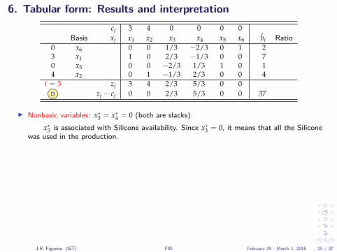
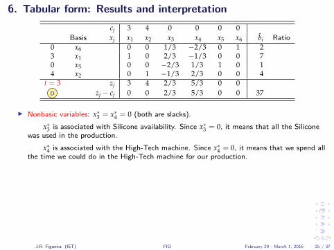
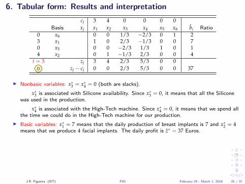
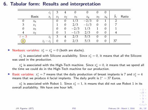
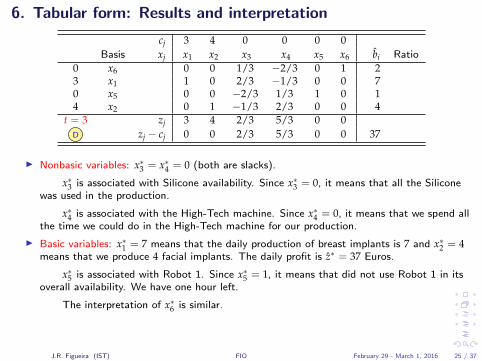
Part
More on Simplex Algorithm

Contents
1. Introduction
2. Linear Programming (LP)
3. The Primal Simplex Method
4. Initial Primal Simplex Tableau
5. Iteration t of Primal Simplex Tableau
6. More results
7. A Primal Simplex Algorithm
Contents
1. Introduction
2. Linear Programming (LP)
3. The Primal Simplex Method
4. Initial Primal Simplex Tableau
5. Iteration t of Primal Simplex Tableau
6. More results
7. A Primal Simplex Algorithm
Contents
1. Introduction
2. Linear Programming (LP)
3. The Primal Simplex Method
4. Initial Primal Simplex Tableau
5. Iteration t of Primal Simplex Tableau
6. More results
7. A Primal Simplex Algorithm
Contents
1. Introduction
2. Linear Programming (LP)
3. The Primal Simplex Method
4. Initial Primal Simplex Tableau
5. Iteration t of Primal Simplex Tableau
6. More results
7. A Primal Simplex Algorithm
Contents
1. Introduction
2. Linear Programming (LP)
3. The Primal Simplex Method
4. Initial Primal Simplex Tableau
5. Iteration t of Primal Simplex Tableau
6. More results
7. A Primal Simplex Algorithm
Contents
1. Introduction
2. Linear Programming (LP)
3. The Primal Simplex Method
4. Initial Primal Simplex Tableau
5. Iteration t of Primal Simplex Tableau
6. More results
7. A Primal Simplex Algorithm
Contents
1. Introduction
2. Linear Programming (LP)
3. The Primal Simplex Method
4. Initial Primal Simplex Tableau
5. Iteration t of Primal Simplex Tableau
6. More results
7. A Primal Simplex Algorithm

1. Introduction
Introduction
I Let us consider again the canonical forms.
I Devise a general tabular form.
I Look at some theoretical results.
I Analyze the data.
I Check for the algorithm.
J.R. Figueira (IST) FIO February 29 - March 1, 2016 28 / 37
1. Introduction
Introduction
I Let us consider again the canonical forms.
I Devise a general tabular form.
I Look at some theoretical results.
I Analyze the data.
I Check for the algorithm.
J.R. Figueira (IST) FIO February 29 - March 1, 2016 28 / 37
1. Introduction
Introduction
I Let us consider again the canonical forms.
I Devise a general tabular form.
I Look at some theoretical results.
I Analyze the data.
I Check for the algorithm.
J.R. Figueira (IST) FIO February 29 - March 1, 2016 28 / 37
1. Introduction
Introduction
I Let us consider again the canonical forms.
I Devise a general tabular form.
I Look at some theoretical results.
I Analyze the data.
I Check for the algorithm.
J.R. Figueira (IST) FIO February 29 - March 1, 2016 28 / 37
1. Introduction
Introduction
I Let us consider again the canonical forms.
I Devise a general tabular form.
I Look at some theoretical results.
I Analyze the data.
I Check for the algorithm.
J.R. Figueira (IST) FIO February 29 - March 1, 2016 28 / 37
1. Introduction
Introduction
I Let us consider again the canonical forms.
I Devise a general tabular form.
I Look at some theoretical results.
I Analyze the data.
I Check for the algorithm.
J.R. Figueira (IST) FIO February 29 - March 1, 2016 28 / 37
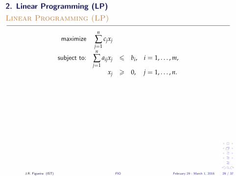
2. Linear Programming (LP)
Linear Programming (LP)
maximizen
∑j=1
cjxj
subject to:n
∑j=1
aijxj 6 bi, i = 1, . . . , m,
xj > 0, j = 1, . . . , n.
Or, by adding the slack variables, xn+1, . . . , xn+i, . . . , xn+m:
maximizen
∑j=1
cjxj
subject to:n
∑j=1
aijxj + xn+i = bi, i = 1, . . . , m,
xj > 0, j = 1, . . . , n + m.
J.R. Figueira (IST) FIO February 29 - March 1, 2016 29 / 37
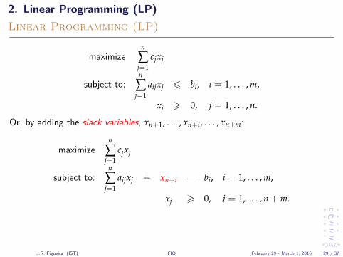
3. The Primal Simplex Method
Primal Simplex Method
Main operations or steps:
1. Pricing: Identifying an entering variable.
2. Ratio test: Identifying a leaving variable.
3. Pivoting: Computing the new row lines and update the basis.
(Algorithms presented next are non-implementable versions of simplex method.)
J.R. Figueira (IST) FIO February 29 - March 1, 2016 30 / 37
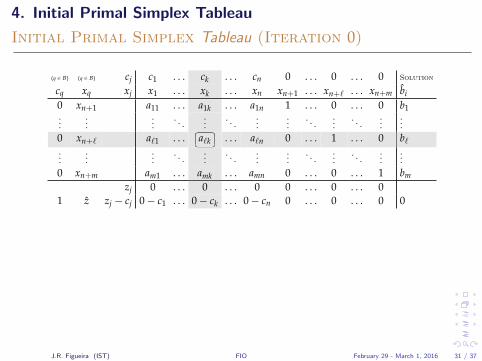
4. Initial Primal Simplex Tableau
Initial Primal Simplex Tableau (Iteration 0)
(q ∈ B) (q ∈ B) cj c1 . . . ck . . . cn 0 . . . 0 . . . 0 Solution
cq xq xj x1 . . . xk . . . xn xn+1 . . . xn+` . . . xn+m bi0 xn+1 a11 . . . a1k . . . a1n 1 . . . 0 . . . 0 b1...
......
. . ....
. . ....
.... . .
.... . .
......
0 xn+` a`1 . . .�� ��a`k . . . a`n 0 . . . 1 . . . 0 b`
......
.... . .
.... . .
......
. . ....
. . ....
...0 xn+m am1 . . . amk . . . amn 0 . . . 0 . . . 1 bm
zj 0 . . . 0 . . . 0 0 . . . 0 . . . 01 z zj − cj 0− c1 . . . 0− ck . . . 0− cn 0 . . . 0 . . . 0 0
I B := (~xn+1, . . . ,~xn+` , . . . ,~xn+m): basis matrix.
I N := (~x1, . . . ,~xk , . . . ,~xn): non-basis matrix.
I B := {n + 1, . . . , n + `, . . . , n + m}: basic variables indexset.
I N := {1, . . . , k, . . . , n}: non-basic variables index set.
I aij: the elements of any tableau, for all i = 1, . . . , m;j = 1, . . . , m + n, w.r.t. B and N.
I (·): position of the variable in the tableau w.r.t. B (forexample, (1) = n + 1).
I zj :=m
∑i=1
c(i) aij, for all j = 1, . . . , m + n.
I z :=m
∑i=1
c(i) bi: objective function value .
I cj := zj − cj: reduced costs (for all j ∈ N ).
I xk: (Dantzig) entering variable such that ck ∈ minj∈N{cj : cj < 0}.
I x(`): leaving variable such that ∆` ∈ mini=1,...,m
{bi/aik : aik > 0}.
I a`k(:= a`k): pivoting element.
I L` := L`/a`k.
I Li := −aik × L` + Li, for all i = 1, . . . , m with i 6= `.
J.R. Figueira (IST) FIO February 29 - March 1, 2016 31 / 37
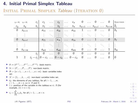
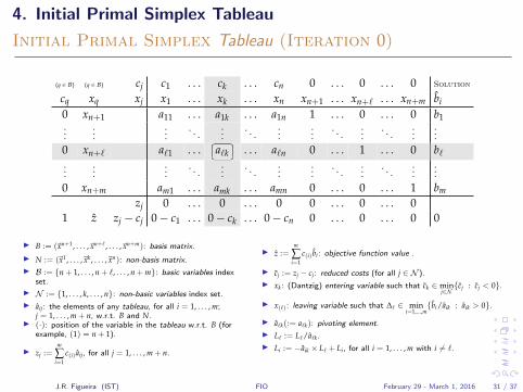
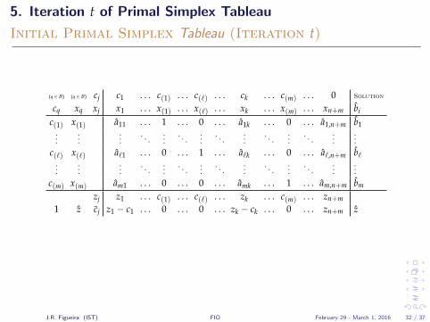
5. Iteration t of Primal Simplex Tableau
Initial Primal Simplex Tableau (Iteration t)
(q ∈ B) (q ∈ B) cj c1 . . . c(1) . . . c(`) . . . ck . . . c(m) . . . 0 Solution
cq xq xj x1 . . . x(1) . . . x(`) . . . xk . . . x(m) . . . xn+m bi
c(1) x(1) a11 . . . 1 . . . 0 . . . a1k . . . 0 . . . a1,n+m b1...
......
. . ....
. . ....
. . ....
. . ....
. . ....
...
c(`) x(`) a`1 . . . 0 . . . 1 . . . a`k . . . 0 . . . a`,n+m b`...
......
. . ....
. . ....
. . ....
. . ....
. . ....
...
c(m) x(m) am1 . . . 0 . . . 0 . . . amk . . . 1 . . . am,n+m bm
zj z1 . . . c(1) . . . c(`) . . . zk . . . c(m) . . . zn+m
1 z cj z1 − c1 . . . 0 . . . 0 . . . zk − ck . . . 0 . . . zn+m z
J.R. Figueira (IST) FIO February 29 - March 1, 2016 32 / 37
6. More results
Fundamental theorems (1)
If at least one basic variable is equal to zero, then such a basic solution iscalled degenerate. Otherwise, it is called nondegenerate.
Definition 5.
A basic feasible solution x is an optimal solution if all reduced costs arenonnegative.
Theorem 5 (Reduced costs optimality condition).
A basic feasible solution x is the unique optimal solution if all reduced costs(associated with the non-basic variables) are strictly positive.
Corollary 5 (Uniqueness of the optimal solution).
J.R. Figueira (IST) FIO February 29 - March 1, 2016 33 / 37
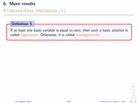
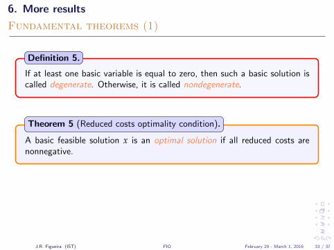
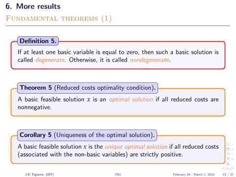
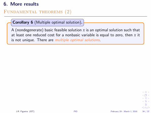
6. More results
Fundamental theorems (2)
A (nondegenerate) basic feasible solution x is an optimal solution such thatat least one reduced cost for a nonbasic variable is equal to zero, then x itis not unique. There are multiple optimal solutions.
Corollary 6 (Multiple optimal solution).
If there is a negative reduced cost, but all the elements of its columnin the Tableau are nonpositive, then the linear programming problem isunbounded.
Theorem 6 (Unboundedness).
If, for a nondegenerate basic feasible solution, there is a negative reducedcost and the corresponding column in the Tableau has a positive compo-nent, then another basic feasible solution can be reached with a bettervalue for the objective function.
Theorem 7 (An improving move).
J.R. Figueira (IST) FIO February 29 - March 1, 2016 34 / 37
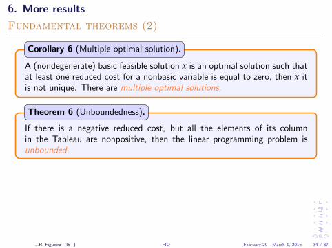
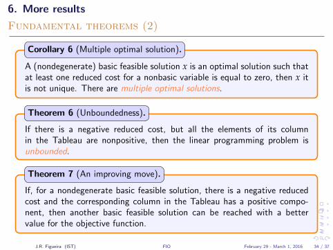
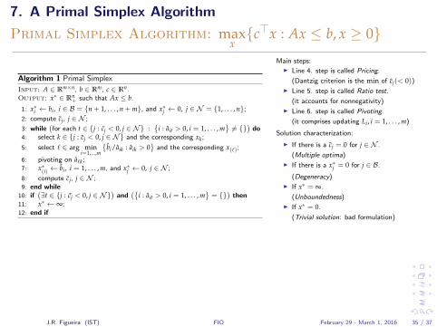
7. A Primal Simplex Algorithm
Primal Simplex Algorithm: maxx{c>x : Ax ≤ b, x ≥ 0}
Algorithm 1 Primal Simplex
Input: A ∈ Rm×n, b ∈ Rm, c ∈ Rn.Output: x∗ ∈ Rn
+ such that Ax ≤ b.
1: x∗i ← bi, i ∈ B = {n + 1, . . . , n + m}, and x∗j ← 0, j ∈ N = {1, . . . , n};2: compute cj, j ∈ N ;
3: while(for each t ∈ {j : cj < 0, j ∈ N} :
{i : ait > 0, i = 1, . . . , m
}6= {}
)do
4: select k ∈ {j : cj < 0, j ∈ N} and the corresponding xk;
5: select ` ∈ arg mini=1,...,m
{bi/aik : aik > 0
}and the corresponding x(`);
6: pivoting on a`k;7: x∗(i) ← bi, i = 1, . . . , m, and x∗j ← 0, j ∈ N ;
8: compute cj, j ∈ N ;9: end while
10: if(∃t ∈ {j : cj < 0, j ∈ N}
)and
({i : ait > 0, i = 1, . . . , m
}= {}
)then
11: x∗ ← ∞;12: end if
Main steps:I Line 4. step is called Pricing.
(Dantzig criterion is the min of cj(< 0))I Line 5. step is called Ratio test.
(it accounts for nonnegativity)
I Line 6. step is called Pivoting.
(it comprises updating Li, i = 1, . . . , m)
Solution characterization:
I If there is a cj = 0 for j ∈ N .
(Multiple optima)
I If there is a x∗j = 0 for j ∈ B.
(Degeneracy)
I If x∗ = ∞.
(Unboundedness)
I If x∗ = 0.
(Trivial solution: bad formulation)
J.R. Figueira (IST) FIO February 29 - March 1, 2016 35 / 37

Part
Bibliography
References
Bazaraa, M., Jarvis, J., and Sherali, H. (1990).
Linear Programming and Network Flows.John Wiley & Sons, New York, USA, second edition.
Goldfarb, D. and Todd, M. J. (1989).
Linear programming.In Nemhauser, G. L., Rinnoy Kan, A. H. G., and Todd, M. J., editors, Optimization, volume 1 of Handbooks in Operations Research andManagement Science, pages 141–170. North Holland, Amsterdam, The Netherlands.
Hillier, F. and Lieberman, G. (2005).
Introduction to Operations Research.The McGraw-Hill Companies, Inc., New York, USA, eighth edition.