Embed Size (px)
DESCRIPTION
finite element 2D
Citation preview
Mul�disciplinary design op�miza�on in computa�onal mechanics
Applica�on case – 2D wing
Piotr Breitkopf 26.11.2014
2
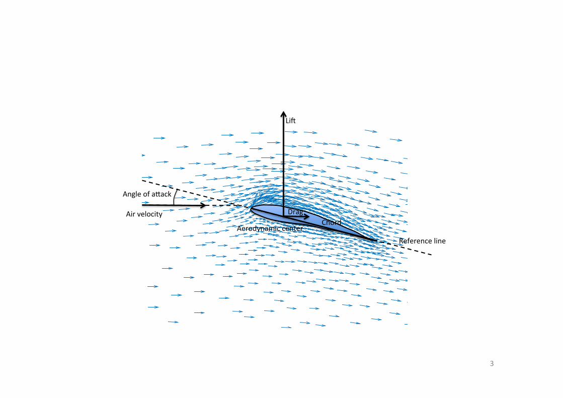
Li�
Drag
Angle of a�ack
Reference line Aerodynamic center
Chord Air velocity
3
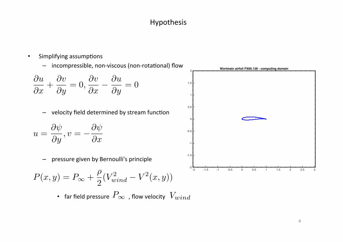
Hypothesis
4
-2 -1.5 -1 -0.5 0 0.5 1 1.5 2 2.5 3-2
-1.5
-1
-0.5
0
0.5
1
1.5
2Wortmain airfoil FX60.126 - computing domain
Simplifying assump�ons – incompressible, non-‐viscous (non-‐rota�onal) flow
– velocity field determined by stream func�on
– pressure given by Bernoulli's principle
far field pressure , flow velocity P1 Vwind
@u
@x+
@v
@y= 0,
@v
@x @u
@y= 0
u =@
@y, v = @
@x
P (x, y) = P1 +⇢
2(V 2
wind V 2(x, y))

Streamlines
5
Curves that are instantaneously tangent to the velocity vector of the flow
n
1
2
0
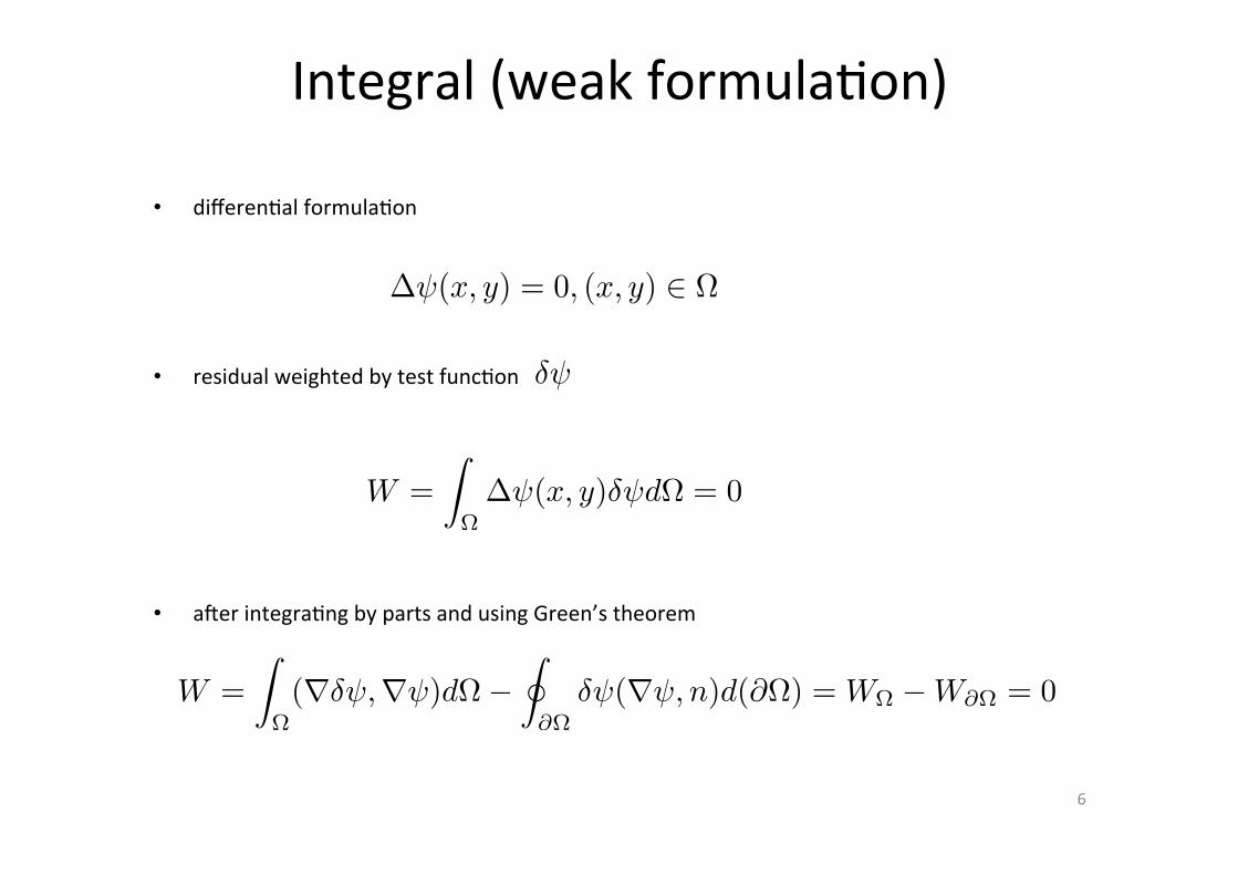
Integral (weak formula�on)
6
W =
Z
⌦
(rδ ,r )d⌦−I
@⌦
δ (r , n)d(@⌦) = W⌦ −W@⌦ = 0
differen�al formula�on
residual weighted by test func�on
a�er integra�ng by parts and using Green’s theorem
δ
W =
Z
⌦
∆ (x, y)δ d⌦ = 0
∆ (x, y) = 0, (x, y) 2 ⌦
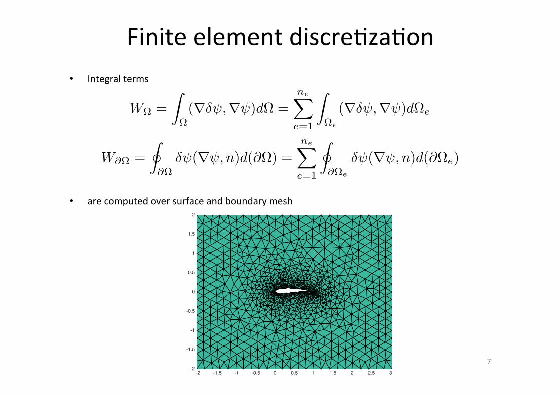
Finite element discre�za�on
7
Integral terms
are computed over surface and boundary mesh
W⌦ =
Z
⌦
(rδ ,r )d⌦ =
neX
e=1
Z
⌦e
(rδ ,r )d⌦e
W@⌦ =
I
@⌦
δ (r , n)d(@⌦) =neX
e=1
I
@⌦e
δ (r , n)d(@⌦e)
-2 -1.5 -1 -0.5 0 0.5 1 1.5 2 2.5 3-2
-1.5
-1
-0.5
0
0.5
1
1.5
2
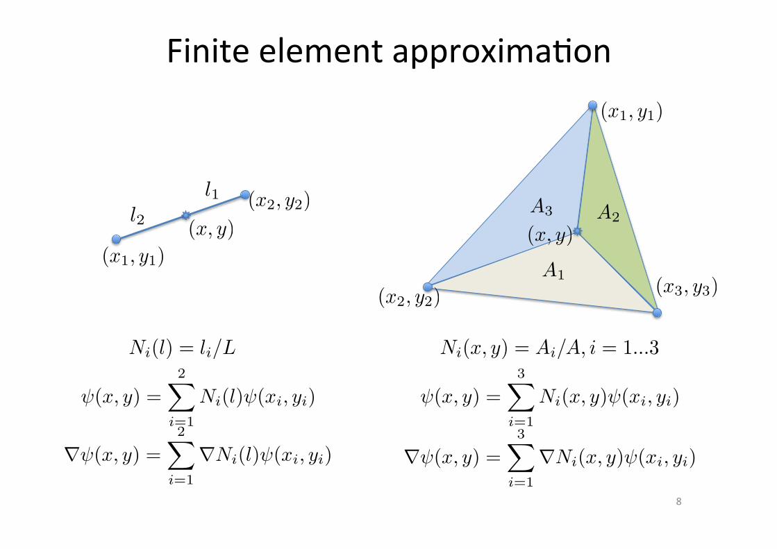
Finite element approxima�on
8
A1
A2A3
(x, y)
(x1, y1)
(x2, y2)(x3, y3)
(x1, y1)
(x2, y2)
(x, y)
l1l2
(x, y) =3X
i=1
Ni(x, y) (xi, yi)
Ni(l) = li/L Ni(x, y) = Ai/A, i = 1...3
(x, y) =2X
i=1
Ni(l) (xi, yi)
r (x, y) =2X
i=1
rNi(l) (xi, yi) r (x, y) =3X
i=1
rNi(x, y) (xi, yi)
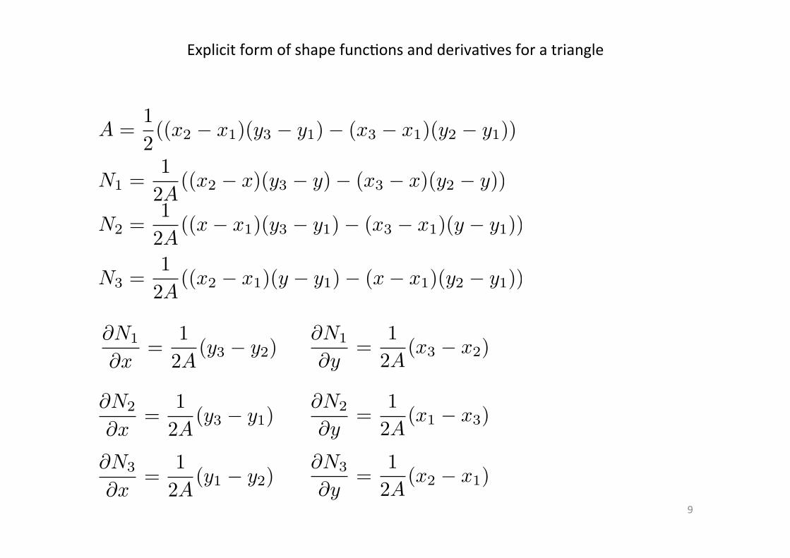
Explicit form of shape func�ons and deriva�ves for a triangle
9
A =1
2((x2 x1)(y3 y1) (x3 x1)(y2 y1))
@N3
@x=
1
2A(y1 y2)
@N3
@y=
1
2A(x2 x1)
N1 =1
2A((x2 x)(y3 y) (x3 x)(y2 y))
N2 =1
2A((x x1)(y3 y1) (x3 x1)(y y1))
@N1
@y=
1
2A(x3 x2)
@N2
@x=
1
2A(y3 y1)
@N2
@y=
1
2A(x1 x3)
N3 =1
2A((x2 x1)(y y1) (x x1)(y2 y1))
@N1
@x=
1
2A(y3 y2)

Surface term
10
Be =1
2A
y2 y3 y3 y1 y1 y2x3 x2 x1 x3 x2 x1
�
W⌦e= δ T
e Ke e,Ke = ABTB
r (x, y) =3X
i=1
rNi(x, y) i =L
6
y2 − y3 y3 − y1 y1 − y2x3 − x2 x1 − x3 x2 − x1
�2
4 1
2
3
3
5 = Be e
δ e =⇥N1(x, y) N2(x, y) N3(x, y)
⇤2
4δ 1
δ 2
δ 3
3
5
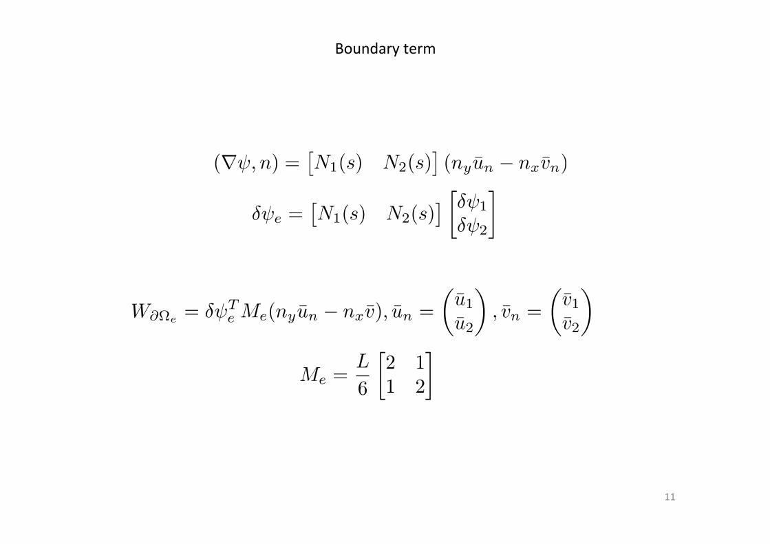
Boundary term
11
Me =L
6
2 11 2
�
W@⌦e= δ T
e Me(nyun nxv), un =
✓u1
u2
◆, vn =
✓v1v2
◆
(r , n) =⇥N1(s) N2(s)
⇤(nyun − nxvn)
δ e =⇥N1(s) N2(s)
⇤ δ 1
δ 2
�
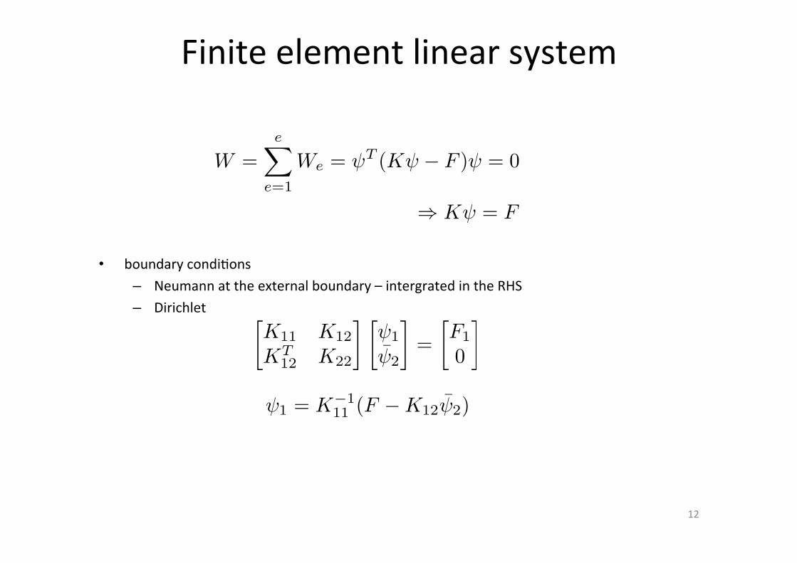
Finite element linear system
12
W =
eX
e=1
We = T (K − F ) = 0
) K = F
boundary condi�ons – Neumann at the external boundary – intergrated in the RHS – Dirichlet
1 = K111 (F K12 2)
K11 K12
KT12 K22
� 1
2
�=
F1
0
�
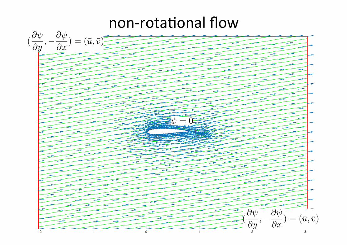
non-‐rota�onal flow
13 -2 -1 0 1 2 3
= 0
(@
@y,@
@x) = (u, v)
(@
@y,@
@x) = (u, v)
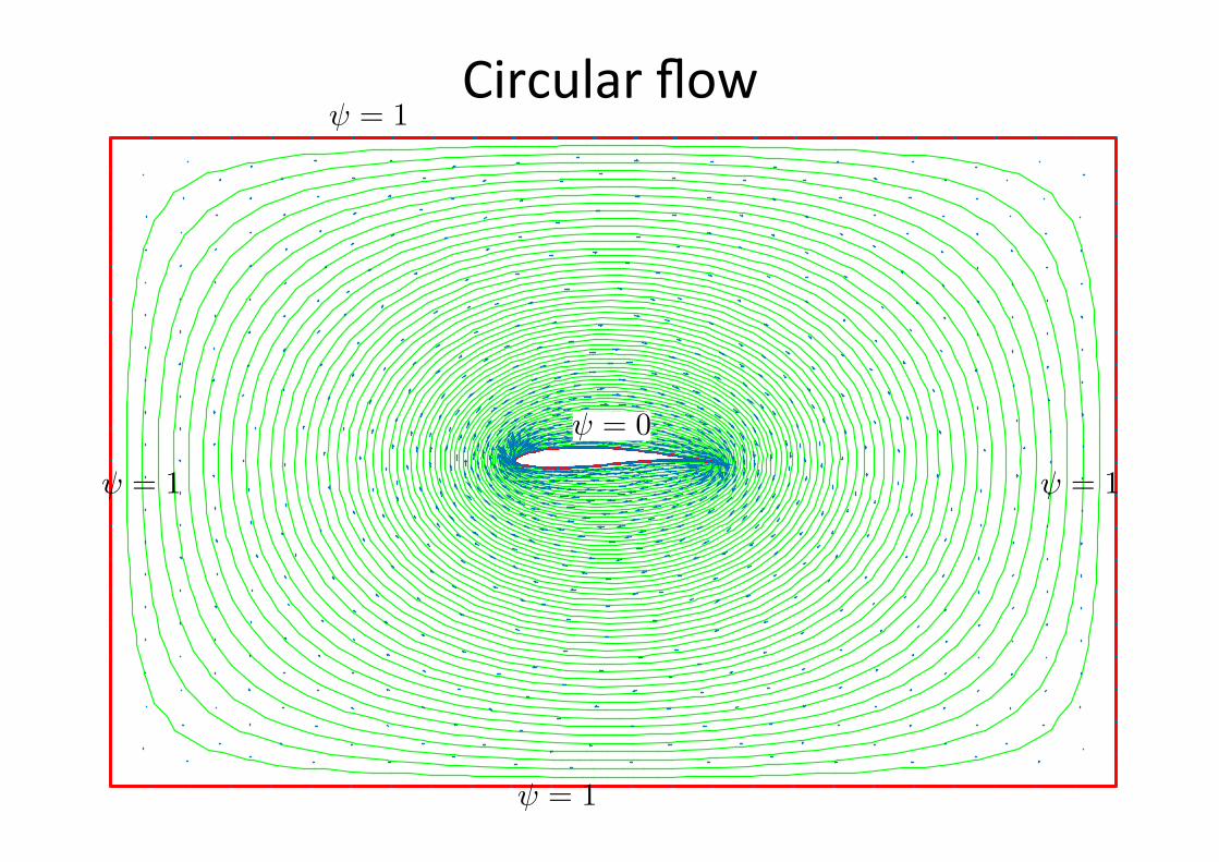
Circular flow
14
= 0
= 1 = 1
= 1
= 1
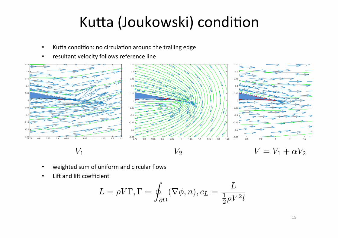
Ku�a (Joukowski) condi�on
15
0.8 0.9 1 1.1 1.2-0.25
-0.2
-0.15
-0.1
-0.05
0
0.05
0.1
0.15
0.2
0.25 p g
0.75 0.8 0.85 0.9 0.95 1 1.05 1.1 1.15 1.2 1.25-0.25
-0.2
-0.15
-0.1
-0.05
0
0.05
0.1
0.15
0.2
0.25 y
0.75 0.8 0.85 0.9 0.95 1 1.05 1.1 1.15 1.2 1.2-0.25
-0.2
-0.15
-0.1
-0.05
0
0.05
0.1
0.15
0.2
0.25 y
V = V1 + ↵V2V1 V2
Ku�a condi�on: no circula�on around the trailing edge resultant velocity follows reference line
weighted sum of uniform and circular flows Li� and li� coefficient
L = ⇢V , =
I
@⌦
(rφ, n), cL =L
12⇢V
2l
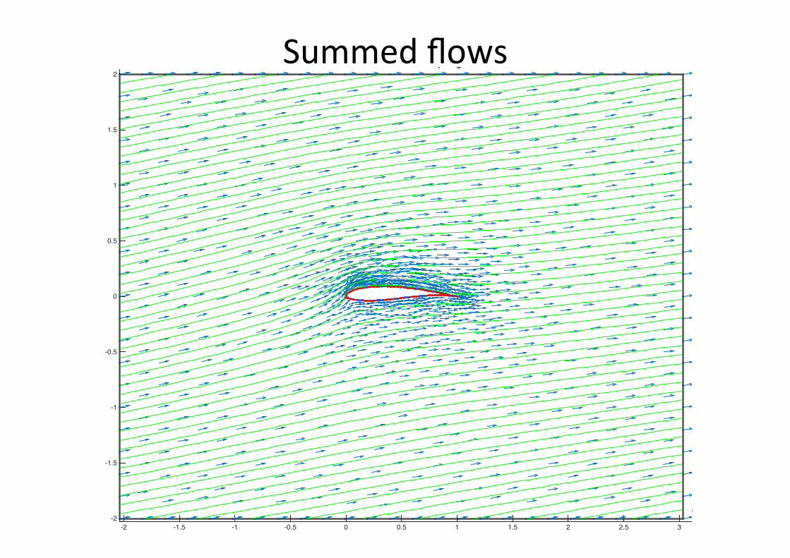
Summed flows
16 -2 -1.5 -1 -0.5 0 0.5 1 1.5 2 2.5 3
-2
-1.5
-1
-0.5
0
0.5
1
1.5
2 p g
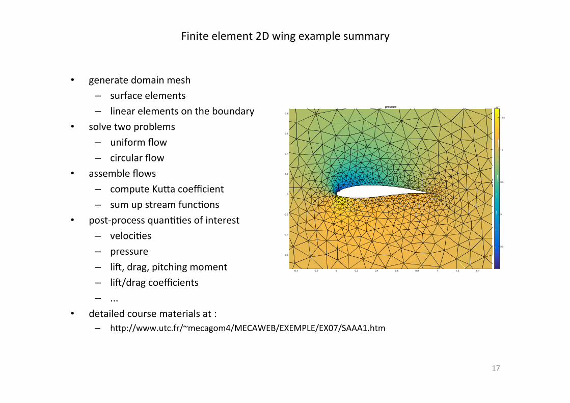
Finite element 2D wing example summary
17
-0.4 -0.2 0 0.2 0.4 0.6 0.8 1 1.2 1.4
-0.6
-0.4
-0.2
0
0.2
0.4
0.6
0.8
pressure #104
8.5
9
9.5
10
10.5
generate domain mesh – surface elements – linear elements on the boundary
solve two problems – uniform flow – circular flow
assemble flows – compute Ku�a coefficient – sum up stream func�ons
post-‐process quan��es of interest – veloci�es – pressure – li�, drag, pitching moment – li�/drag coefficients – ...
detailed course materials at : – h�p://www.utc.fr/~mecagom4/MECAWEB/EXEMPLE/EX07/SAAA1.htm

![Angewandte Umweltsystemanalyse: [1.0ex] Finite-Differenzen ... · V6: Implizite FDM25.05.2012 2D implizite FDM Der Ausdruck K=S = entspricht dem Di usivit atskoe zienten (Uberpr ufen](https://img.pdfslide.tips/doc/110x75/5e0424f046e8a351f5541cc7/angewandte-umweltsystemanalyse-10ex-finite-differenzen-v6-implizite-fdm25052012.jpg)


![Finite [Mayjune2013]](https://img.pdfslide.tips/doc/110x75/55cf8d2c5503462b1392af25/finite-mayjune2013.jpg)