FIR Filter Design via Sp ectral F - Engineeringvandenbe/publications/magdes.pdf · 1. FIR Filter Design via Sp ectral F actorization and Con v ex Optimization 3 maxim um allo w ed

1. FIR Filter Design via Spectral Factorization and Convex Optimization 1

FIR Filter Design via Spectral

Factorization and Convex

Optimization

Shao-Po WuStephen BoydLieven Vandenberghe

ABSTRACT We consider the design of �nite impulse response (FIR) �lters

subject to upper and lower bounds on the frequency response magnitude.

The associated optimization problems, with the �lter coe�cients as the

variables and the frequency response bounds as constraints, are in general

nonconvex. Using a change of variables and spectral factorization, we can

pose such problems as linear or nonlinear convex optimization problems. As

a result we can solve them e�ciently (and globally) by recently developed

interior-point methods. We describe applications to �lter and equalizer de-

sign, and the related problem of antenna array weight design.

� To appear as Chapter 1 of Applied Computational Control, Signal and Commu-

nications, Biswa Datta editor, Birkhauser, 1997.

� The paper is also available at URL http://www-isl.stanford.edu/people/boyd

and from anonymous FTP to isl.stanford.edu in pub/boyd/reports.

2 Shao-Po Wu, Stephen Boyd, Lieven Vandenberghe

1 Introduction

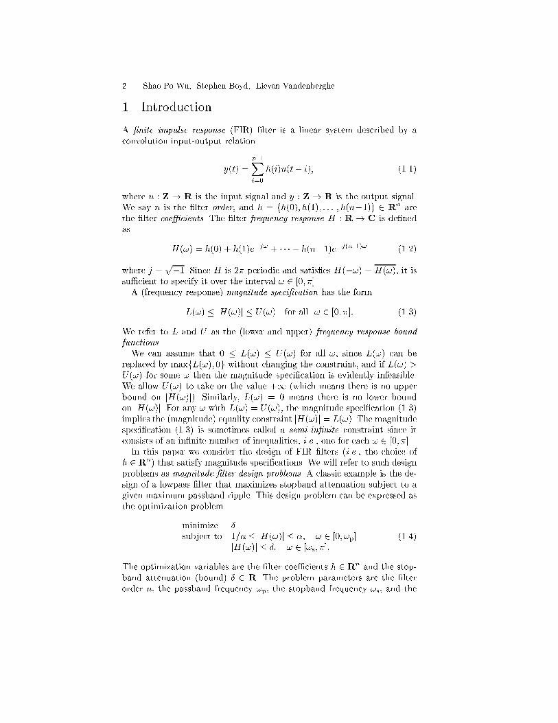
A �nite impulse response (FIR) �lter is a linear system described by aconvolution input-output relation

y(t) =

n�1Xi=0

h(i)u(t� i); (1.1)

where u : Z ! R is the input signal and y : Z ! R is the output signal.We say n is the �lter order, and h =

�h(0); h(1); : : : ; h(n�1)

�2 Rn are

the �lter coe�cients. The �lter frequency response H : R ! C is de�nedas

H(!) = h(0) + h(1)e�j! + � � �+ h(n�1)e�j(n�1)! (1.2)

where j =p�1. Since H is 2� periodic and satis�es H(�!) = H(!), it is

su�cient to specify it over the interval ! 2 [0; �].A (frequency response) magnitude speci�cation has the form

L(!) � jH(!)j � U(!) for all ! 2 [0; �]: (1.3)

We refer to L and U as the (lower and upper) frequency response bound

functions.

We can assume that 0 � L(!) � U(!) for all !, since L(!) can bereplaced by maxfL(!); 0g without changing the constraint, and if L(!) >U(!) for some ! then the magnitude speci�cation is evidently infeasible.We allow U(!) to take on the value +1 (which means there is no upperbound on jH(!)j). Similarly, L(!) = 0 means there is no lower boundon jH(!)j. For any ! with L(!) = U(!), the magnitude speci�cation (1.3)implies the (magnitude) equality constraint jH(!)j = L(!). The magnitudespeci�cation (1.3) is sometimes called a semi-in�nite constraint since itconsists of an in�nite number of inequalities, i.e., one for each ! 2 [0; �].In this paper we consider the design of FIR �lters (i.e., the choice of

h 2 Rn) that satisfy magnitude speci�cations. We will refer to such designproblems as magnitude �lter design problems. A classic example is the de-sign of a lowpass �lter that maximizes stopband attenuation subject to agiven maximum passband ripple. This design problem can be expressed asthe optimization problem

minimize �

subject to 1=� � jH(!)j � �; ! 2 [0; !p]jH(!)j � �; ! 2 [!s; �]:

(1.4)

The optimization variables are the �lter coe�cients h 2 Rn and the stop-band attenuation (bound) � 2 R. The problem parameters are the �lterorder n, the passband frequency !p, the stopband frequency !s, and the


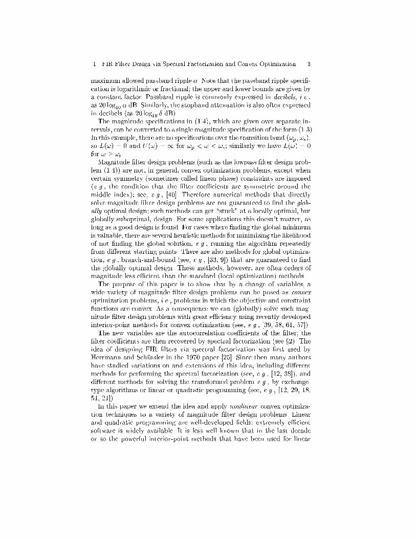
maximum allowed passband ripple �. Note that the passband ripple speci�-cation is logarithmic or fractional; the upper and lower bounds are given bya constant factor. Passband ripple is commonly expressed in decibels, i.e.,as 20 log10 � dB. Similarly, the stopband attenuation is also often expressedin decibels (as 20 log10 � dB).The magnitude speci�cations in (1.4), which are given over separate in-

tervals, can be converted to a single magnitude speci�cation of the form (1.3).In this example, there are no speci�cations over the transition band (!p; !s),so L(!) = 0 and U(!) = 1 for !p < ! < !s; similarly we have L(!) = 0for ! � !s.Magnitude �lter design problems (such as the lowpass �lter design prob-

lem (1.4)) are not, in general, convex optimization problems, except whencertain symmetry (sometimes called linear phase) constraints are imposed(e.g., the condition that the �lter coe�cients are symmetric around themiddle index); see, e.g., [40]. Therefore numerical methods that directlysolve magnitude �lter design problems are not guaranteed to �nd the glob-ally optimal design; such methods can get \stuck" at a locally optimal, butglobally suboptimal, design. For some applications this doesn't matter, aslong as a good design is found. For cases where �nding the global minimumis valuable, there are several heuristic methods for minimizing the likelihoodof not �nding the global solution, e.g., running the algorithm repeatedlyfrom di�erent starting points. There are also methods for global optimiza-tion, e.g., branch-and-bound (see, e.g., [33, 9]) that are guaranteed to �ndthe globally optimal design. These methods, however, are often orders ofmagnitude less e�cient than the standard (local optimization) methods.The purpose of this paper is to show that by a change of variables, a

wide variety of magnitude �lter design problems can be posed as convexoptimization problems, i.e., problems in which the objective and constraintfunctions are convex. As a consequence we can (globally) solve such mag-nitude �lter design problems with great e�ciency using recently developedinterior-point methods for convex optimization (see, e.g., [39, 58, 61, 57]).The new variables are the autocorrelation coe�cients of the �lter; the

�lter coe�cients are then recovered by spectral factorization (see x2). Theidea of designing FIR �lters via spectral factorization was �rst used byHerrmann and Sch�ussler in the 1970 paper [25]. Since then many authorshave studied variations on and extensions of this idea, including di�erentmethods for performing the spectral factorization (see, e.g., [12, 38]), anddi�erent methods for solving the transformed problem e.g., by exchange-type algorithms or linear or quadratic programming (see, e.g., [12, 29, 18,51, 21]).In this paper we extend the idea and apply nonlinear convex optimiza-

tion techniques to a variety of magnitude �lter design problems. Linearand quadratic programming are well-developed �elds; extremely e�cientsoftware is widely available. It is less well known that in the last decadeor so the powerful interior-point methods that have been used for linear


and quadratic programming have been extended to handle a huge variety ofnonlinear convex optimization problems (see, e.g., [39, 56, 36]). Making useof convex optimization methods more general than linear or quadratic pro-gramming preserves the solution e�ciency, and allows us to handle a widerclass of problems, e.g., problems with logarithmic (decibel) objectives.We close this introduction by comparing magnitude �lter design, the

topic of this paper, with complex Chebychev design, in which the speci�ca-tions have the general form

jH(!)�D(!)j � U(!) for all ! 2 [0; �];

where D : [0; �] ! C is a desired or target frequency response, andU : [0; �] ! R (with U(!) � 0) is a frequency-dependent weighting func-tion. Complex Chebychev design problems, unlike the magnitude designproblems addressed in this paper, are generally convex, directly in thevariables h; see, e.g., [17, 45].


2 Spectral factorization

The autocorrelation coe�cients associated with the �lter (1.1) are de�nedas

r(t) =

n�1Xi=�n+1

h(i)h(i+ t); t 2 Z; (1.5)

where we interpret h(t) as zero for t < 0 or t > n � 1. Since r(t) =r(�t) and r(t) = 0 for t � n, it su�ces to specify the autocorrelationcoe�cients for t = 0; : : : ; n�1. With some abuse of notation, we will writethe autocorrelation coe�cients as a vector r =

�r(0); : : : ; r(n�1)

�2 Rn.

The Fourier transform of the autocorrelation coe�cients is

R(!) =Xt2Z

r(t)e�j!t = r(0) +

n�1Xt=1

2r(t) cos!t = jH(!)j2; (1.6)

i.e., the squared magnitude of the �lter frequency response. We will usethe autocorrelation coe�cients r 2 R

n as the optimization variable inplace of the �lter coe�cients h 2 R

n. This change of variables has tobe handled carefully, since the transformation from �lter coe�cients intoautocorrelation coe�cients is not one-to-one, and not all vectors r 2 Rn

are the autocorrelation coe�cients of some �lter.From (1.6) we immediately have a necessary condition for r to be the

autocorrelation coe�cients of some �lter: R must satisfy R(!) � 0 for all !.It turns out that this condition is also su�cient: The spectral factorizationtheorem (see, e.g., [4, ch9]) states that there exists an h 2 Rn such thatr 2 Rn is the autocorrelation coe�cients of h if and only if

R(!) � 0 for all ! 2 [0; �]: (1.7)

The process of determining �lter coe�cients h whose autocorrelationcoe�cients are r, given an r 2 Rn that satis�es the spectral factorizationcondition (1.7), is called spectral factorization. Some widely used spectralfactorization methods are summarized in the appendix.Let us now return to magnitude �lter design problems. The magnitude

speci�cation (1.3) can be expressed in terms of the autocorrelation coe�-cients r as

L(!)2 � R(!) � U(!)2 for all ! 2 [0; �]:

Of course, we must only consider r that are the autocorrelation coe�cientsof some h, so we must append the spectral factorization condition to obtain:

L(!)2 � R(!) � U(!)2; R(!) � 0 for all ! 2 [0; �]: (1.8)


These conditions are equivalent to the original magnitude speci�cationsin the following sense: there exists an h that satis�es (1.3) if and only ifthere exists an r that satis�es (1.8). Note that the spectral factorizationconstraint R(!) � 0 is redundant: it is implied by L(!)2 � R(!).For each !, the constraints in (1.8) are a pair of linear inequalities in the

vector r; hence the overall constraint (1.8) is convex in r. In many cases, thischange of variable converts the original, nonconvex optimization problemin the variable h into an equivalent, convex optimization problem in thevariable r.As a simple example, consider the classical lowpass �lter design prob-

lem (1.4) described above. We can pose it in terms of r as

minimize ~�subject to 1=�2 � R(!) � �2; ! 2 [0; !p]

R(!) � ~�; ! 2 [!s; �]R(!) � 0; ! 2 [0; �]:

(1.9)

(~� here corresponds to �2 in the original problem (1.4).)In contrast to the original lowpass �lter design problem (1.4), the prob-

lem (1.9) is a convex optimization problem in the variables r 2 Rn and~� 2 R. In fact it is a semi-in�nite linear program, since the objective islinear and the constraints are semi-in�nite, i.e., a pair of linear inequalitiesfor each !.

3 Convex semi-in�nite optimization

In this paper we encounter convex optimization problems of the generalform

minimize f0(x)subject to Ax = b;

fi(x) � 0; i = 1; : : : ;m;

gi(x; !) � 0; ! 2 [0; �]; i = 1; : : : ; p;

(1.10)

where x 2 Rk is the optimization variable, f0; : : : ; fm : Rk ! R are

convex functions, and for each ! 2 [0; �], gi(x; !) are convex functions ofx. Note the three types of constraints: Ax = b are the equality constraints;fi(x) � 0 are the (ordinary) inequality constraints; and gi(x; !) � 0 forall ! are the semi-in�nite inequality constraints. If the objective functionf0 is identically zero, the problem (1.10) reduces to verifying whether theconstraints are feasible or not, i.e., to a feasibility problem.In the remainder of this section we give a brief discussion of various

methods for handling the semi-in�nite constraints. General semi-in�niteconvex optimization is a well-developed �eld; see for example [8, 44, 7,


27, 26, 41, 47]. While the theory and methods for general semi-in�niteconvex optimization can be technical and complex, our feeling is that thevery special form of the semi-in�nite constraints appearing in �lter designproblems allows them to be solved with no great theoretical or practicaldi�culty.Let us start by pointing out that the semi-in�nite inequality constraint

gi(x; !) � 0 for all ! 2 [0; �]

can be handled by expressing it as the ordinary inequality constraint

hi(x) = sup!2[0;�]

gi(x; !) � 0:

It is easily veri�ed that hi is a convex function of x, since for each !, gi(x; !)is convex in x. (On the other hand, hi is often nondi�erentiable, evenif the functions gi are di�erentiable.) Thus, the semi-in�nite constraintsin (1.10) can be handled by several methods for general (nondi�erentiable)convex optimization, e.g., bundle methods [28], ellipsoid methods [11], orcutting plane methods [30, 23, 46]. What is required in these methods is ane�cient method for evaluating hi and a subgradient at any x. This involvescomputing a frequency � for which gi(x; �) = hi(x). In some problems thiscan be done analytically; in any case it can be found approximately by a(one-dimensional) search over frequency. (See, e.g., [15, 13].)It is also possible to solve some magnitude �lter design problems exactly,

by transforming the semi-in�nite constraints into (�nite-dimensional) con-straints that involve linear matrix inequalities [14, 55, 63], but we will notpursue this idea here.The semi-in�nite constraints can also be approximated in a very straight-

forward way by sampling or discretizing frequency. We choose a set of fre-quencies

0 � !1 � !2 � � � � � !N � �;

often uniformly or logarithmically spaced, and replace the semi-in�niteinequality constraint

gi(x; !) � 0 for all ! 2 [0; �]

with the set of N ordinary inequality constraints

gi(x; !k) � 0 k = 1; : : : ; N:

Note that sampling preserves convexity. When N is su�ciently large, dis-cretization yields a good approximation of the SIP (see [19]). A standardrule of thumb is to choose N � 15n (assuming linear spacing).


As an example consider the lowpass �lter design problem given by (1.9).The discretized approximation has the form

minimize ~�subject to 1=�2 � R(!k) � �2; !k 2 [0; !p]

R(!k) � ~�; !k 2 [!s; �]R(!k) � 0; !k 2 [0; �]:

(1.11)

This is in fact a linear program (LP) with n + 1 variables (r; ~�), and 2Nlinear inequality constraints. One immediate advantage is that existing,e�cient LP software can be used to solve this (discretized) lowpass �lterdesign problem.The reader should note the di�erences between the three variations on the

lowpass �lter design problem. The original problem (1.4) is a semi-in�nite,nonconvex problem. The transformed problem (1.9) is a semi-in�nite butconvex problem, which is equivalent (by change of variables) to the originalproblem (1.4). The transformed and discretized problem (1.11) is an ap-

proximation of the semi-in�nite problem (1.9). It is also a linear program,and so can be solved using standard linear programming codes (or, for evengreater e�ciency, by an interior-point LP solver that exploits the specialproblem structure [16]).Evidently for the discretized problem we can no longer guarantee that the

semi-in�nite constraints are satis�ed between frequency samples. Indeedthe sampled version of the problem is an outer approximation of the originalproblem; its feasible set includes the feasible set of the original problem. Inmany cases this causes no particular harm, especially if N is large. But ifthe spectral factorization condition does not hold, i.e., R(�) < 0 for some� between samples, then spectral factorization breaks down; we cannot�nd a set of �lter coe�cients h that have r as its autocorrelation. Severalmethods can be used to avoid this pitfall. The simplest is to add a smallsafety margin to the sampled version of the spectral factorization condition,i.e., replace it by

R(!k) � �; k = 1; : : : ; N (1.12)

where � is small and positive. This can be done in an ad hoc way, byincreasing � (and re-solving the problem) until the spectral factorization ofR is successful. If N is large this will occur when � is small.We can also analyze the approximation error induced by discretization

by bounding the variation of the functions gi(x; !) for ! between samples.To give a very simple example, assume we use uniform frequency sampling,i.e., !k = (k � 1=2)�=N , k = 1; : : : ; N . We assume we have (or impose)some bound on the size of h, say,

khk =ph(0)2 + � � �+ h(n� 1)2 �M:


Thus, r(0) = khk2 �M2, and a standard result shows that jr(t)j �M2 forall t.Now let ! be any frequency in [0; �] and let !k denote the nearest sam-

pling frequency, so that j! � !kj � �=(2N). We have

jR(!)�R(!k)j =��n�1Xt=1

2r(t)(cos!t� cos!kt)

��

� 4M2

n�1Xt=1

�� sin j! � !kjt�� 4M2

n�1Xt=1

��! � !k�� t �M2n(n�1)�=N

Thus, the intersample error cannot exceedM2n(n�1)�=N (which evidentlyconverges to zero as N !1). For example, if we take � =M2n(n�1)�=Nin (1.12), then it is guaranteed that the (semi-in�nite) spectral factorizationcondition (1.7) will be met. The bound developed here is very simple, andonly meant to give the general idea; far more sophisticated bounds can bederived; see, e.g., [19, x3.7].Let us mention several reasons why simple discretization works very well

in practice and is widely used. First of all, its computational cost is notprohibitive. Even when special structure (see below) is not exploited, thecomplexity of solving the discretized problem grows approximately as alinear function of N , so making N large (to get a good discretized approx-imation) incurs only a linear increase in computation required.When uniform frequency sampling is used, the fast Fourier transform

can be used to great advantage to speed up many of the computations ininterior-point methods. In [16] the authors demonstrate that FIR designproblems with 1000s of variables and 10000s of constraints can be solved intens of seconds on a small workstation, by exploiting the special structureof the discretized problems.Finally, we should point out that frequency sampling plays a key role

in the more sophisticated methods for handling semi-in�nite constraints.Indeed, most of the more sophisticated algorithms for SIPs solve a sequenceof discretized problems with carefully chosen frequency samples (see, e.g.,[26, 47].In the remainder of this paper, we will pose problems �rst as convex,

semi-in�nite problems. We then either give the sampled version, or pointout if it has a special form such as LP. The sampled versions can be thoughtof as approximations (which are probably more than adequate for practicaldesigns) or as subproblems that arise in sophisticated algorithms that han-dle the semi-in�nite constraints exactly. The numerical results given in thispaper were obtained from (�ne) discretizations, using the nonlinear convexprogramming solver SDPSOL [62].


!

jH(!)j

�

1=�

�

!p !s �

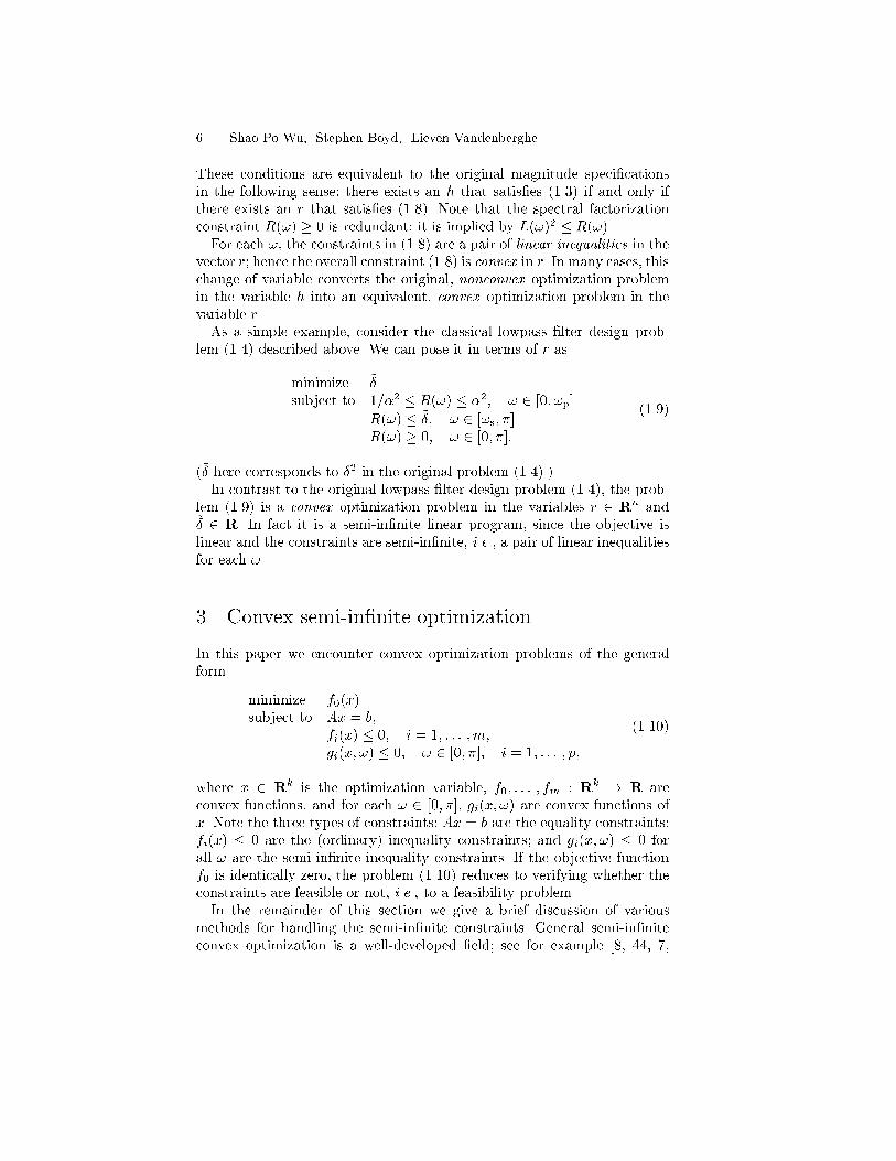
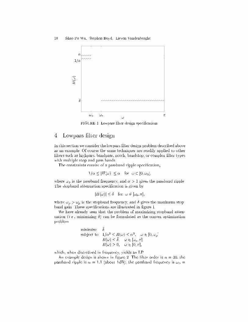
FIGURE 1. Lowpass �lter design speci�cations.

4 Lowpass �lter design

In this section we consider the lowpass �lter design problem described aboveas an example. Of course the same techniques are readily applied to other�lters such as highpass, bandpass, notch, bandstop, or complex �lter typeswith multiple stop and pass bands.The constraints consist of a passband ripple speci�cation,

1=� � jH(!)j � � for ! 2 [0; !p];

where !p is the passband frequency, and � > 1 gives the passband ripple.The stopband attenuation speci�cation is given by

jH(!)j � � for ! 2 [!s; �];

where !p > !p is the stopband frequency, and � gives the maximum stop-band gain. These speci�cations are illustrated in �gure 1.We have already seen that the problem of maximizing stopband atten-

uation (i.e., minimizing �) can be formulated as the convex optimizationproblem

minimize ~�subject to 1=�2 � R(!) � �2; ! 2 [0; !p]

R(!) � ~�; ! 2 [!s; �]R(!) � 0; ! 2 [0; �];

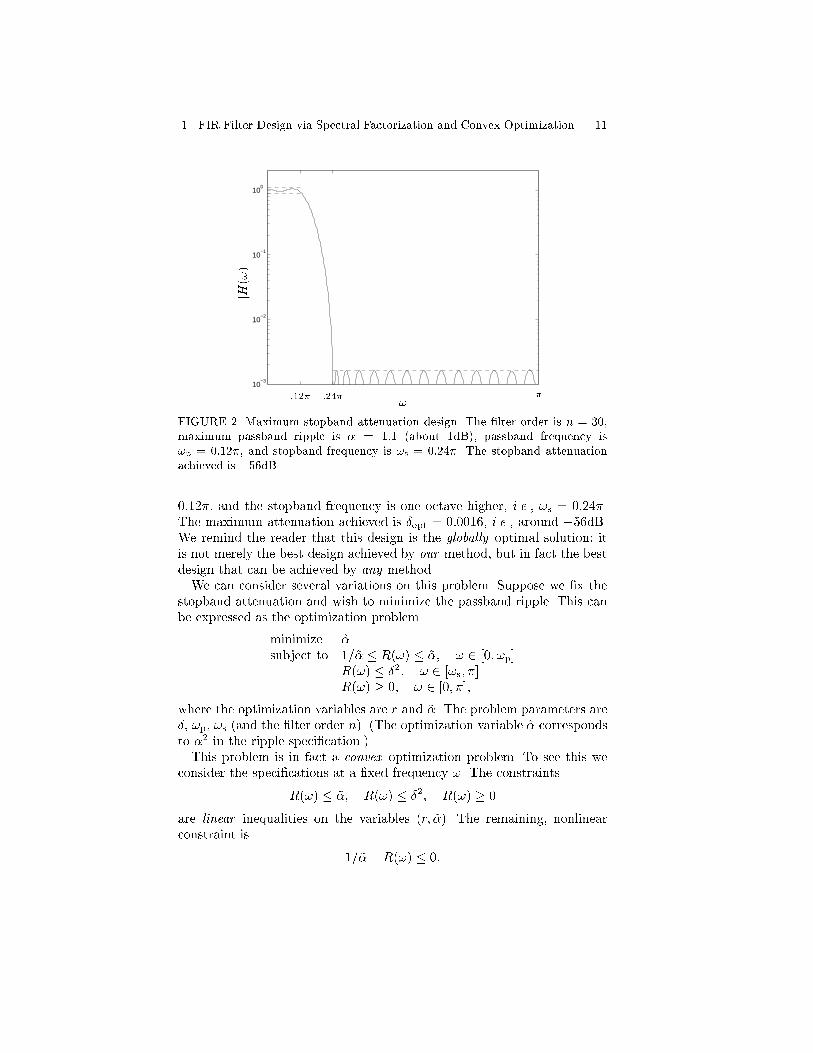
which, when discretized in frequency, yields an LP.An example design is shown in �gure 2. The �lter order is n = 30, the

passband ripple is � = 1:1 (about 1dB), the passband frequency is !p =


10−3

10−2

10−1

100

!

jH(!)j

:12� :24� �

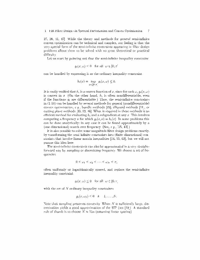
FIGURE 2. Maximum stopband attenuation design. The �lter order is n = 30,

maximum passband ripple is � = 1:1 (about 1dB), passband frequency is

!p = 0:12�, and stopband frequency is !s = 0:24�. The stopband attenuation

achieved is �56dB.

0:12�, and the stopband frequency is one octave higher, i.e., !s = 0:24�.The maximum attenuation achieved is �opt = 0:0016, i.e., around �56dB.We remind the reader that this design is the globally optimal solution: itis not merely the best design achieved by our method, but in fact the bestdesign that can be achieved by any method.We can consider several variations on this problem. Suppose we �x the

stopband attenuation and wish to minimize the passband ripple. This canbe expressed as the optimization problem

minimize ~�subject to 1=~� � R(!) � ~�; ! 2 [0; !p]

R(!) � �2; ! 2 [!s; �]R(!) � 0; ! 2 [0; �];

where the optimization variables are r and ~�. The problem parameters are�, !p, !s (and the �lter order n). (The optimization variable ~� correspondsto �2 in the ripple speci�cation.)This problem is in fact a convex optimization problem. To see this we

consider the speci�cations at a �xed frequency !. The constraints

R(!) � ~�; R(!) � �2; R(!) � 0

are linear inequalities on the variables (r; ~�). The remaining, nonlinearconstraint is

1=~��R(!) � 0:


The function 1=~��R(!) can be veri�ed to be convex in the variables (r; ~�)(since ~� > 0). Indeed, when sampled this problem can be very e�cientlysolved as a second-order cone program (SOCP); see [36, x3.3] and [35].Note that passband ripple minimization (in dB) cannot be solved (directly)by linear programming; it can, however, be solved by nonlinear convexoptimization.We can formulate other variations on the lowpass �lter design problem

by �xing the passband ripple and stopband attenuation, and optimizingover one of the remaining parameters. For example we can minimize thestopband frequency !s (with the other parameters �xed). This problem isquasiconvex ; it is readily and e�ciently solved using bisection on !s andsolving the resulting convex feasibility problems (which, when sampled,become LP feasibility problems). Similarly, !p (which is quasiconcave) canbe maximized, or the �lter order (which is quasiconvex) can be minimized.It is also possible to include several types of constraints on the slope of

the magnitude of the frequency response. We start by considering upperand lower bounds on the absolute slope, i.e.,

a � djH(!)jd!

� b:

This can be expressed as

a � dR(!)1=2

d!=

dR=d!

2pR(!)

� b;

which (since R(!) is constrained to be positive) we can rewrite as

2pR(!)a � dR=d! � 2

pR(!)b:

Now we introduce the assumption that a � 0 and b � 0. The inequalitiescan be written

2apR(!)� dR=d! � 0; dR=d! � b

pR(!) � 0: (1.13)

Since R(!) is a linear function of r (and positive),pR(!) is a concave

function of r. Hence the functions apR(!) and �b

pR(!) are convex (since

a � 0 and b � 0). Thus, the inequalities (1.13) are convex (since dR=d! is alinear function of r). When discretized, this constraint can be handled viaSOCP. As a simple application we can design a lowpass �lter subject to theadditional constraint that the frequency response magnitude is monotonicdecreasing.Let us now turn to the more classical speci�cation of frequency response

slope, which involves the logarithmic slope:

a � djH jd!

!

jH(!)j � b:


(The logarithmic slope is commonly given in units of dB/octave or dB/decade.)This can be expressed as

a � (1=2)dR

d!

!

R(!)� b;

which in turn can be expressed as a pair of linear inequalities on r:

2R(!)a=! � dR

d!� 2R(!)b=!:

Note that we can incorporate arbitrary upper and lower bounds on thelogarithmic slope, including equality constraints (when a = b). Thus, con-straints on logarithmic slope (in dB/octave) are readily handled.

5 Log-Chebychev approximation

Consider the problem of designing an FIR �lter so that its frequency re-sponse magnitude best approximates a target or desired function, in thesense of minimizing the maximum approximation error in decibels (dB).We can formulate this problem as

minimize sup!2[0;�]

�� log jH(!)j � logD(!)�� (1.14)

where D : [0; �] ! R is the desired frequency response magnitude (withD(!) > 0 for all !). We call (1.14) a logarithmic Chebychev approximationproblem, since it is a minimax (Chebychev) problem on a logarithmic scale.We can express the log-Chebychev problem (1.14) as

minimize �

subject to 1=� � R(!)=D(!)2 � �; ! 2 [0; �];R(!) � 0; ! 2 [0; �]

where the variables are r 2 Rn and � 2 R. This is a convex optimizationproblem (as described above), e�ciently solved, for example, as an SOCP.Simple variations on this problem include the addition of other constraints,or a frequency-weighted log-Chebychev objective.As an example we consider the design of a 1=f spectrum-shaping �lter,

which is used to generate 1=f noise by �ltering white noise through anFIR �lter. The goal is to approximate the magnitude D(!) = !�1=2 overa frequency band [!a; !b]. If white noise (i.e., a process with spectrumSu(!) = 1) is passed through such a �lter, the output spectrum Sy willsatisfy Sy(!) � 1=! over [!a; !b]. This signal can be used to simulate 1=fnoise (e.g., in a circuit or system simulation) or as a test signal in audioapplications (where it is called pink noise [54]).


10−1

100

101

!

jH(!)j

:01� :1� �

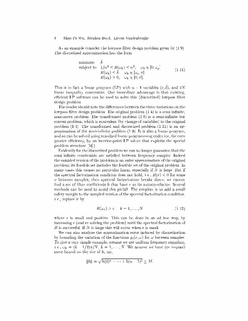
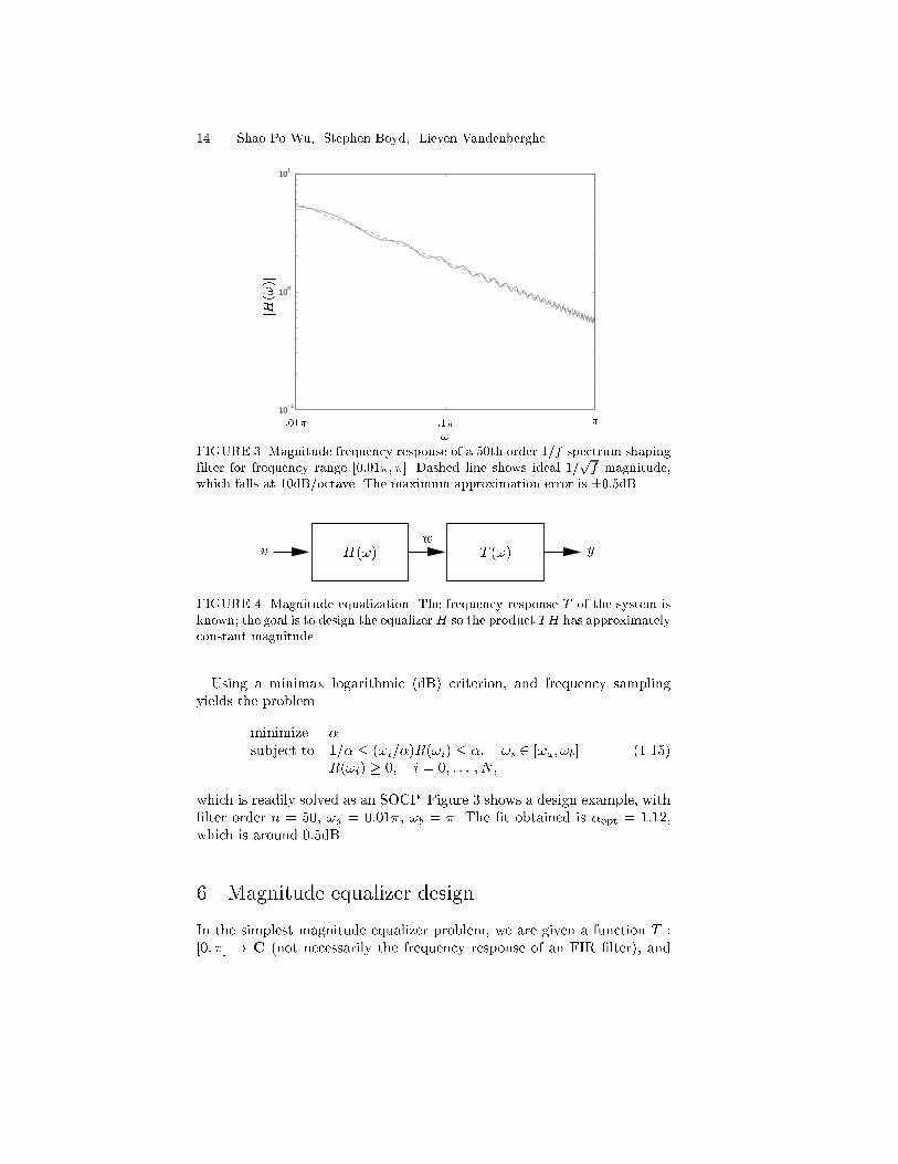
FIGURE 3. Magnitude frequency response of a 50th order 1=f spectrum shaping

�lter for frequency range [0:01�; �]. Dashed line shows ideal 1=pf magnitude,

which falls at 10dB/octave. The maximum approximation error is �0:5dB.

v H(!)w

T (!) y

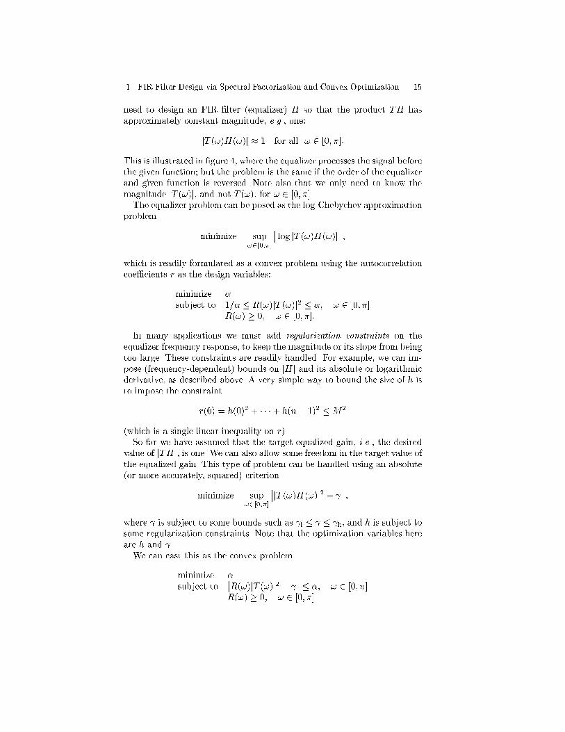
FIGURE 4. Magnitude equalization. The frequency response T of the system is

known; the goal is to design the equalizerH so the product TH has approximately

constant magnitude.

Using a minimax logarithmic (dB) criterion, and frequency samplingyields the problem

minimize �

subject to 1=� � (!i=�)R(!i) � �; !i 2 [!a; !b]R(!i) � 0; i = 0; : : : ; N;

(1.15)

which is readily solved as an SOCP. Figure 3 shows a design example, with�lter order n = 50, !a = 0:01�, !b = �. The �t obtained is �opt = 1:12,which is around 0:5dB.

6 Magnitude equalizer design

In the simplest magnitude equalizer problem, we are given a function T :[0; �] ! C (not necessarily the frequency response of an FIR �lter), and


need to design an FIR �lter (equalizer) H so that the product TH hasapproximately constant magnitude, e.g., one:

jT (!)H(!)j � 1 for all ! 2 [0; �]:

This is illustrated in �gure 4, where the equalizer processes the signal beforethe given function; but the problem is the same if the order of the equalizerand given function is reversed. Note also that we only need to know themagnitude jT (!)j, and not T (!), for ! 2 [0; �].The equalizer problem can be posed as the log-Chebychev approximation

problem


�� log jT (!)H(!)j�� ;

which is readily formulated as a convex problem using the autocorrelationcoe�cients r as the design variables:

minimize �

subject to 1=� � R(!)jT (!)j2 � �; ! 2 [0; �]R(!) � 0; ! 2 [0; �]:

In many applications we must add regularization constraints on theequalizer frequency response, to keep the magnitude or its slope from beingtoo large. These constraints are readily handled. For example, we can im-pose (frequency-dependent) bounds on jH j and its absolute or logarithmicderivative, as described above. A very simple way to bound the size of h isto impose the constraint

r(0) = h(0)2 + � � �+ h(n� 1)2 �M2

(which is a single linear inequality on r).So far we have assumed that the target equalized gain, i.e., the desired

value of jTH j, is one. We can also allow some freedom in the target value ofthe equalized gain. This type of problem can be handled using an absolute(or more accurately, squared) criterion


��jT (!)H(!)j2 � �� ;

where is subject to some bounds such as l � � h, and h is subject tosome regularization constraints. Note that the optimization variables hereare h and .We can cast this as the convex problem

minimize �

subject to��R(!)jT (!)j2 �

�� ; ! 2 [0; �]R(!) � 0; ! 2 [0; �]


0 0.5 1 1.5 2 2.5 310

−3

10−2

10−1

100

101

102

jT(!)H(!)j

!

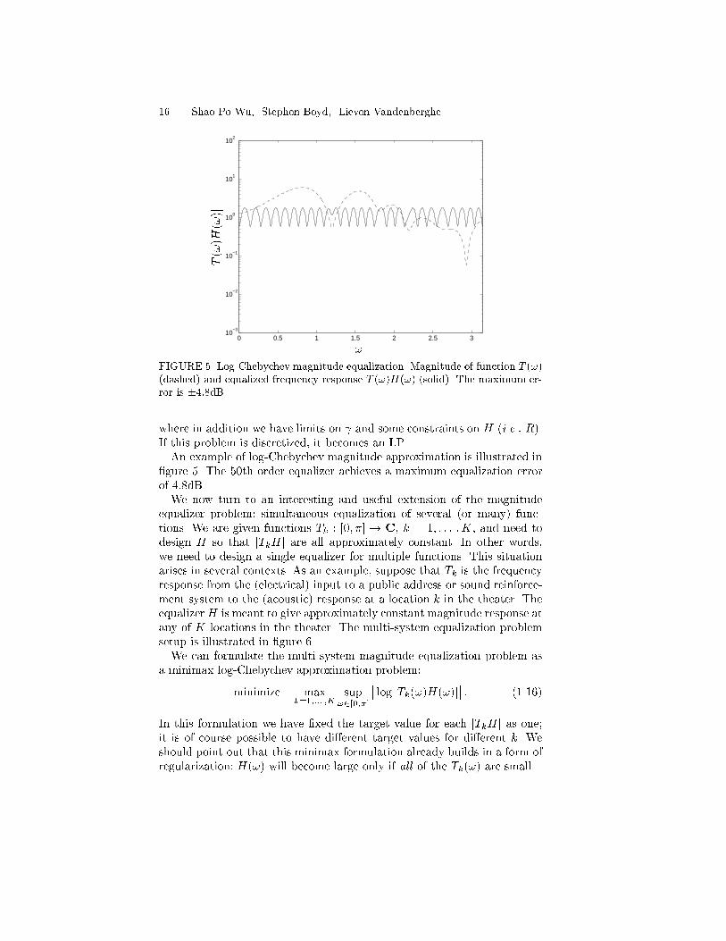
FIGURE 5. Log-Chebychev magnitude equalization. Magnitude of function T (!)

(dashed) and equalized frequency response T (!)H(!) (solid). The maximum er-

ror is �4:8dB.

where in addition we have limits on and some constraints on H (i.e., R).If this problem is discretized, it becomes an LP.An example of log-Chebychev magnitude approximation is illustrated in

�gure 5. The 50th order equalizer achieves a maximum equalization errorof 4:8dB.We now turn to an interesting and useful extension of the magnitude

equalizer problem: simultaneous equalization of several (or many) func-tions. We are given functions Tk : [0; �] ! C, k = 1; : : : ;K, and need todesign H so that jTkH j are all approximately constant. In other words,we need to design a single equalizer for multiple functions. This situationarises in several contexts. As an example, suppose that Tk is the frequencyresponse from the (electrical) input to a public address or sound reinforce-ment system to the (acoustic) response at a location k in the theater. TheequalizerH is meant to give approximately constant magnitude response atany of K locations in the theater. The multi-system equalization problemsetup is illustrated in �gure 6.We can formulate the multi-system magnitude equalization problem as

a minimax log-Chebychev approximation problem:

minimize maxk=1;::: ;K

sup!2[0;�]

�� log jTk(!)H(!)j�� : (1.16)

In this formulation we have �xed the target value for each jTkH j as one;it is of course possible to have di�erent target values for di�erent k. Weshould point out that this minimax formulation already builds in a form ofregularization: H(!) will become large only if all of the Tk(!) are small.


v H(!)w

264

T1(!)...

TK(!)

375

y1

y2

yK

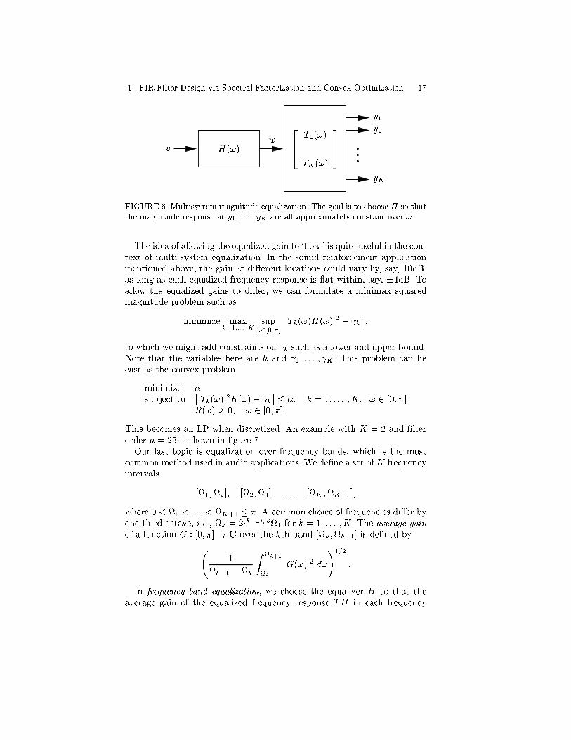
FIGURE 6. Multisystem magnitude equalization. The goal is to choose H so that

the magnitude response at y1; : : : ; yK are all approximately constant over !.

The idea of allowing the equalized gain to ` oat' is quite useful in the con-text of multi-system equalization. In the sound reinforcement applicationmentioned above, the gain at di�erent locations could vary by, say, 10dB,as long as each equalized frequency response is at within, say, �4dB. Toallow the equalized gains to di�er, we can formulate a minimax squaredmagnitude problem such as

minimize maxk=1;::: ;K

sup!2[0;�]

��jTk(!)H(!)j2 � k�� ;

to which we might add constraints on k such as a lower and upper bound.Note that the variables here are h and 1; : : : ; K . This problem can becast as the convex problem

minimize �

subject to��jTk(!)j2R(!)� k

�� ; k = 1; : : : ;K; ! 2 [0; �]R(!) � 0; ! 2 [0; �]:

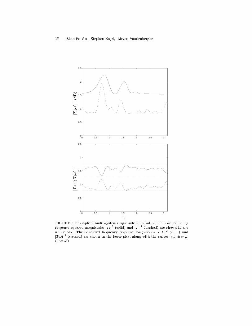
This becomes an LP when discretized. An example with K = 2 and �lterorder n = 25 is shown in �gure 7.Our last topic is equalization over frequency bands, which is the most

common method used in audio applications. We de�ne a set of K frequencyintervals

[1;2]; [2;3]; : : : [K ;K+1];

where 0 < 1 < : : : < K+1 � �. A common choice of frequencies di�er byone-third octave, i.e., k = 2(k�1)=31 for k = 1; : : : ;K. The average gainof a function G : [0; �]! C over the kth band [k;k+1] is de�ned by

1

k+1 �k

Z k+1

k

jG(!)j2 d!!1=2

:

In frequency band equalization, we choose the equalizer H so that theaverage gain of the equalized frequency response TH in each frequency


0 0.5 1 1.5 2 2.5 30

0.5

1

1.5

2

2.5

jTi(!)j2(dB)

0 0.5 1 1.5 2 2.5 30

0.5

1

1.5

2

2.5

jTi(!)H(!)j2

!

FIGURE 7. Example of multi-system magnitude equalization. The two frequency

response squared magnitudes jT1j2 (solid) and jT2j2 (dashed) are shown in the

upper plot. The equalized frequency response magnitudes jT1Hj2 (solid) and

jT2Hj2 (dashed) are shown in the lower plot, along with the ranges opt � �opt

(dotted).


band is approximately the same. Using a log-Chebychev (minimax dB)criterion for the gains and r as the variable, we can express this equalizationproblem as

minimize �

subject to 1=� � 1k+1�k

R k+1k

R(!)jT (!)j2 d! � �; k = 1; : : : ;K;

R(!) � 0; ! 2 [0; �]:

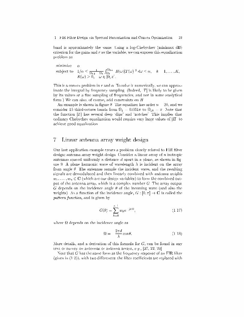
This is a convex problem in r and �. To solve it numerically, we can approx-imate the integral by frequency sampling. (Indeed, jT j is likely to be givenby its values at a �ne sampling of frequencies, and not in some analyticalform.) We can also, of course, add constraints on H .An example is shown in �gure 8. The equalizer has order n = 20, and we

consider 15 third-octave bands from 1 = 0:031� to 16 = �. Note thatthe function jT j has several deep `dips' and `notches'. This implies thatordinary Chebychev equalization would require very large values of jH j toachieve good equalization.

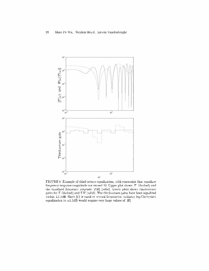
7 Linear antenna array weight design

Our last application example treats a problem closely related to FIR �lterdesign: antenna array weight design. Consider a linear array of n isotropicantennas spaced uniformly a distance d apart in a plane, as shown in �g-ure 9. A plane harmonic wave of wavelength � is incident on the arrayfrom angle �. The antennas sample the incident wave, and the resultingsignals are demodulated and then linearly combined with antenna weights

w1; : : : ; wn 2 C (which are our design variables) to form the combined out-put of the antenna array, which is a complex number G. The array outputG depends on the incidence angle � of the incoming wave (and also theweights). As a function of the incidence angle, G : [0; �] ! C is called thepattern function, and is given by

G(�) =

n�1Xk=0

wke�jk; (1.17)

where depends on the incidence angle as

= �2�d

�cos �: (1.18)

More details, and a derivation of this formula for G, can be found in anytext or survey on antennas or antenna arrays, e.g., [37, 22, 20].Note that G has the same form as the frequency response of an FIR �lter

(given in (1.2)), with two di�erences: the �lter coe�cients are replaced with


10−1

100

10−3

10−2

10−1

100

101

jT(!)jandjH(!)T(!)j

10−1

100

10−3

10−2

10−1

100

101

Third-octavegain

!

FIGURE 8. Example of third-octave equalization, with constraint that equalizer

frequency response magnitude not exceed 10. Upper plot shows jT j (dashed) andthe equalized frequency response jTHj (solid). Lower plots shows third-octave

gains for T (dashed) and TH (solid). The third-octave gains have been equalized

within �1:1dB. Since jT j is small at several frequencies, ordinary log-Chebychev

equalization to �1:1dB would require very large values of jHj.


�

�

2d

FIGURE 9. Linear antenna array of antennas (shown as dots), with spacing d,

in the plane. A plane wave with wavelength � is incident from angle �.

the antenna array weights (which can be complex), and the \frequency"variable is related to the incidence angle � by (1.18).If we de�ne H : [��; �]! C as

H() =

n�1Xk=0

wke�jk;

then we have G(�) = H(). H is then the frequency response of anFIR �lter with (complex) coe�cients w1; : : : ; wn. Since H does not sat-isfy H(�) = H() (as the frequency response of an FIR �lter with realcoe�cients does), we must specify H over 2 [��; �].For � 2 [0; �], is monotonically increasing function of �, which we will

denote , i.e., (�) = �2�d=� cos �. As the incidence angle � varies from 0to �, the variable = (�) varies over the range �2�d=�. To simplify thediscussion below, we make the (common) assumption that d < �=2, i.e.,the element spacing is less than one half wavelength. This implies that for� 2 [0; �], (�) = is restricted to an interval inside [��; �]. An interval

�min � � � �max;

where �min; �max 2 [0; �], transforms under (1.18) to the correspondinginterval

min � � max;

where min = (�min) and max = (�max), which lie in [��; �]. (Theimportance of this will soon become clear.)By analogy with the FIR �lter design problem, we can de�ne an antenna

pattern magnitude speci�cation as

L(�) � jG(�)j � U(�) for all � 2 [0; �]: (1.19)


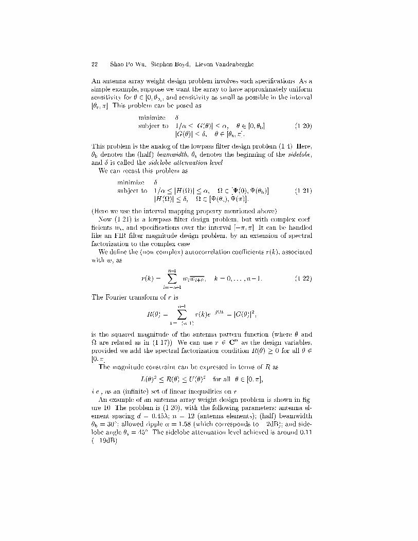
An antenna array weight design problem involves such speci�cations. As asimple example, suppose we want the array to have approximately uniformsensitivity for � 2 [0; �b], and sensitivity as small as possible in the interval[�s; �]. This problem can be posed as

minimize �

subject to 1=� � jG(�)j � �; � 2 [0; �b]jG(�)j � �; � 2 [�s; �]:

(1.20)

This problem is the analog of the lowpass �lter design problem (1.4). Here,�b denotes the (half) beamwidth, �s denotes the beginning of the sidelobe,and � is called the sidelobe attenuation level.We can recast this problem as

minimize �

subject to 1=� � jH()j � �; 2 [(0);(�b)]jH()j � �; 2 [(�s);(�)]:

(1.21)

(Here we use the interval mapping property mentioned above).Now (1.21) is a lowpass �lter design problem, but with complex coef-

�cients wi, and speci�cations over the interval [��; �]. It can be handledlike an FIR �lter magnitude design problem, by an extension of spectralfactorization to the complex case.We de�ne the (now complex) autocorrelation coe�cients r(k), associated

with w, as

r(k) =

n�1Xi=�n+1

wiwi+k ; k = 0; : : : ; n�1: (1.22)

The Fourier transform of r is

R(�) =

n�1Xk=�(n�1)

r(k)e�jk = jG(�)j2;

is the squared magnitude of the antenna pattern function (where � and are related as in (1.17)). We can use r 2 Cn as the design variables,provided we add the spectral factorization condition R(�) � 0 for all � 2[0; �].The magnitude constraint can be expressed in terms of R as

L(�)2 � R(�) � U(�)2 for all � 2 [0; �];

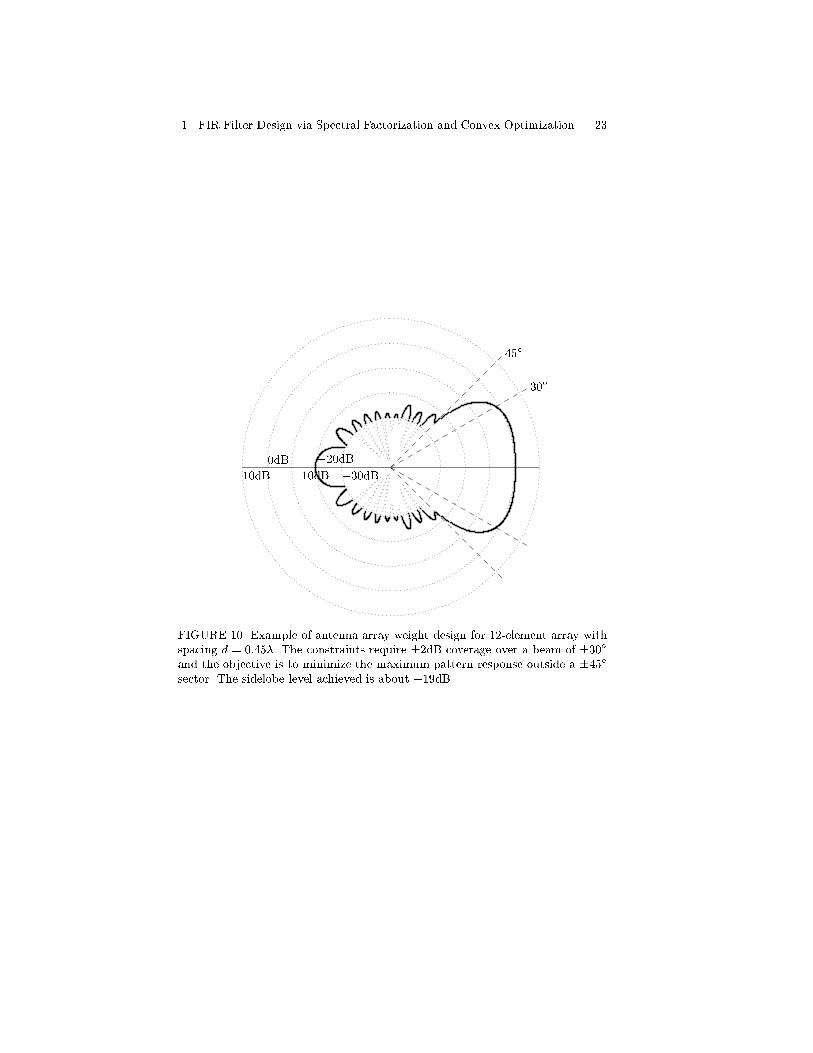
i.e., as an (in�nite) set of linear inequalities on r.An example of an antenna array weight design problem is shown in �g-

ure 10. The problem is (1.20), with the following parameters: antenna el-ement spacing d = 0:45�; n = 12 (antenna elements); (half) beamwidth�b = 30�; allowed ripple � = 1:58 (which corresponds to �2dB); and side-lobe angle �s = 45�. The sidelobe attenuation level achieved is around 0:11(�19dB).


30�

45�

10dB

0dB

�10dB�20dB

�30dB

FIGURE 10. Example of antenna array weight design for 12-element array with

spacing d = 0:45�. The constraints require �2dB coverage over a beam of �30�

and the objective is to minimize the maximum pattern response outside a �45�

sector. The sidelobe level achieved is about �19dB.


8 Conclusions

We have shown that a variety of magnitude FIR �lter design problemscan be formulated, in terms of the autocorrelation coe�cients, as (pos-sibly nonlinear) convex semi-in�nite optimization problems. As a result,the globally optimal solution can be e�ciently computed. By consideringnonlinear convex optimization problems, we can solve a number of prob-lems of practical interest, e.g., minimax decibel problems, with an e�ciencynot much less than standard methods that rely on, for example, linear orquadratic programming.

Acknowledgments: This research was supported in part by AFOSR (un-der F49620-95-1-0318), NSF (under ECS-9222391 and EEC-9420565), andMURI (under F49620-95-1-0525). The authors would like to thank BabakHassibi, Laurent El Ghaoui, and Herv�e Lebret for very helpful discussionsand comments. They also thank Paul Van Dooren for bringing reference [59]to their attention.

9 References

[1] F. A. Aliyev, B. A. Bordyug, and V. B. Larin. Factorization of poly-nomial matrices and separation of rational matrices. Soviet Journal

of Computer and Systems Sciences, 28(6):47{58, 1990.

[2] F. A. Aliyev, B. A. Bordyug, and V. B. Larin. Discrete generalizedalgebraic Riccati equations and polynomial matrix factorization. Syst.Control Letters, 18:49{59, 1992.

[3] B. Anderson. An algebraic solution to the spectral factorization prob-lem. IEEE Trans. Aut. Control, AC-12(4):410{414, Aug. 1967.

[4] B. Anderson and J. B. Moore. Optimal Filtering. Prentice-Hall, 1979.

[5] B. Anderson and S. Vongpanitlerd. Network analysis and synthesis: a

modern systems theory approach. Prentice-Hall, 1973.

[6] B. D. O. Anderson, K. L. Hitz, and N. D. Diem. Recursive algo-rithm for spectral factorization. IEEE Transactions on Circuits and

Systems, 21:742{750, 1974.

[7] E. J. Anderson and P. Nash. Linear Programming in In�nite-

Dimensional Spaces: Theory and Applications. John Wiley & Sons,1987.

[8] E. J. Anderson and A. B. Philpott, editors. In�nite Programming.Springer-Verlag Lecture Notes in Economics and Mathematical Sys-tems, Sept. 1984.


[9] V. Balakrishnan and S. Boyd. Global optimization in control systemanalysis and design. In C. T. Leondes, editor, Control and Dynamic

Systems: Advances in Theory and Applications, volume 53. AcademicPress, New York, New York, 1992.

[10] F. L. Bauer. Ein direktes Iterationsverfahren zur Hurwitz-Zerlegungeines Polynoms. Arch. Elek. �Ubertr., 9:844{847, 1955.

[11] R. G. Bland, D. Goldfarb, and M. J. Todd. The ellipsoid method: Asurvey. Operations Research, 29(6):1039{1091, 1981.

[12] R. Boite and H. Leich. A new procedure for the design of high orderminimum phase FIR digital or CCD �lters. Signal Processing, 3:101{108, 1981.

[13] S. Boyd and C. Barratt. Linear Controller Design: Limits of Perfor-mance. Prentice-Hall, 1991.

[14] S. Boyd, L. El Ghaoui, E. Feron, and V. Balakrishnan. Linear Matrix

Inequalities in System and Control Theory, volume 15 of Studies in

Applied Mathematics. SIAM, Philadelphia, PA, June 1994.

[15] S. Boyd and L. Vandenberghe. Introduction to convex op-timization with engineering applications. Course Notes, 1997.http://www-leland.stanford.edu/class/ee364/.

[16] S. Boyd, L. Vandenberghe, and M. Grant. E�cient convex optimiza-tion for engineering design. In Proceedings IFAC Symposium on Ro-

bust Control Design, pages 14{23, Sept. 1994.

[17] D. Burnside and T. W. Parks. Optimal design of �r �lters with thecomplex chebyshev error criteria. IEEE Transactions on Signal Pro-

cessing, 43(3):605{616, March 1995.

[18] X. Chen and T. W. Parks. Design of optimal minimum phase FIR�lters by direct factorization. Signal Processing, 10:369{383, 1986.

[19] E. W. Cheney. Introduction to Approximation Theory. Chelsea Pub-lishing Company, New York, second edition, 1982.

[20] D. K. Cheng. Optimization techniques for antenna arrays. Proceedingsof the IEEE, 59(12):1664{1674, Dec. 1971.

[21] J. O. Coleman. The Use of the FF Design Language for the Linear

Programming Design of Finite Impulse Response Digital Filters for

Digital Communication and Other Applications. PhD thesis, Unversityof Washington, 1991.

[22] R. S. Elliott. Antenna Theory and Design. Prentice-Hall, 1981.


[23] J. Elzinga and T. Moore. A central cutting plane algorithm for theconvex programming problem. Math. Program. Studies, 8:134{145,1975.

[24] P. A. Fuhrmann. Elements of factorization theory from a polynomialpoint of view. In H. Nijmeijer and J. M. Schumacher, editors, ThreeDecades of Mathematical System Theory, volume 135 of Lecture Notesin Control and Information Sciences, pages 148{178. Springer Verlag,1989.

[25] O. Herrmann and H. W. Sch�ussler. Design of nonrecursive digital�lters with minimum-phase. Electronic Letter, 6:329{330, 1970.

[26] R. Hettich. A review of numerical methods for semi-in�nite program-ming and applications. In A. V. Fiacco and K. O. Kortanek, editors,Semi-In�nite Programming and Applications, pages 158{178. Springer,Berlin, 1983.

[27] R. Hettich and K. O. Kortanek. Semi-in�nite programming: theory,methods and applications. SIAM Review, 35:380{429, 1993.

[28] J.-B. Hiriart-Urruty and C. Lemar�echal. Convex Analysis and Mini-

mization Algorithms II: Advanced Theory and Bundle Methods, volume306 of Grundlehren der mathematischen Wissenschaften. Springer-Verlag, New York, 1993.

[29] Y. Kamp and C. J. Wellekens. Optimal design of minimum-phase FIR�lters. IEEE Trans. Acoust., Speech, Signal Processing, 31(4):922{926,1983.

[30] J. E. Kelley. The cutting-plane method for solving convex programs.J. Soc. Indust. Appl. Math, 8(4):703{712, Dec. 1960.

[31] P. Lancaster and L. Rodman. Solutions of the continuous and discretetime algebraic Riccati equations: a review. In S. Bittanti, A. J. Laub,and J. C. Willems, editors, The Riccati equation, pages 11{51. SpringerVerlag, Berlin, Germany, 1991.

[32] V. B. Larin. An algorithm for factoring a matrix polynomial relative toa unit-radius circle. Journal of Automation and Information Sciences,26(1):1{6, 1993.

[33] E. L. Lawler and D. E. Wood. Branch-and-bound methods: A survey.Operations Research, 14:699{719, 1966.

[34] H. Lebret and S. Boyd. Antenna array pattern synthesis via con-vex optimization. IEEE Trans. on Signal Processing, 45(3):526{532,March 1997.


[35] M. S. Lobo, L. Vandenberghe, and S. Boyd. socp: Software for

Second-Order Cone Programming. Information Systems Laboratory,Stanford University, 1997.

[36] M. S. Lobo, L. Vandenberghe, S. Boyd, and H. Lebret. Second-ordercone programming: interior-point methods and engineering applica-tions. Linear Algebra and Appl., 1997. Submitted.

[37] M. T. Ma. Theory and Application of Antenna Arrays. John Wileyand Sons, 1974.

[38] G. A. Mian and A. P. Nainer. A fast procedure to design equirippleminimum-phase FIR �lters. IEEE Trans. Circuits Syst., 29(5):327{331, 1982.

[39] Y. Nesterov and A. Nemirovsky. Interior-point polynomial methods inconvex programming, volume 13 of Studies in Applied Mathematics.SIAM, Philadelphia, PA, 1994.

[40] A. V. Oppenheim and R. W. Schafer. Digital Signal Processing.Prentice-Hall, Englewood Cli�s, N. J., 1970.

[41] E. Panier and A. Tits. A globally convergent algorithm withadaptively re�ned discretization for semi-in�nite optimization prob-lems arising in engineering design. IEEE Trans. Aut. Control, AC-34(8):903{908, 1989.

[42] A. Papoulis. Signal Analysis. McGraw-Hill, New York, 1977.

[43] T. W. Parks and C. S. Burrus. Digital Filter Design. Topics in DigitalSignal Processing. John Wiley & Sons, New York, 1987.

[44] E. Polak. Semi-in�nite optimization in engineering design. In A. Fi-acco and K. Kortanek, editors, Semi-in�nite Programming and Appli-

cations. Springer-Verlag, 1983.

[45] A. W. Potchinkov and R. M. Reemtsen. The design of FIR �lters in thecomplex plane by convex optimization. Signal Processing, 46(2):127{146, Oct. 1995.

[46] R. M. Reemtsen. A cutting-plane method for solving minimax prob-lems in the complex plane. Numerical Algorithms, 2:409{436, 1992.

[47] R. M. Reemtsen. Some outer approximation methods for semi-in�niteoptimization problems. Journal of Computational and Applied Math-

ematics, 53:87{108, 1994.


[48] R. M. Reemtsen and A. W. Potchinkov. FIR �lter design in regard tofrequency response, magnitude, and phase by semi-in�nite program-ming. In J. Guddat, H. T. Jongen, F. Nozicka, G. Still, and F. Twilt,editors, Parametric Optimization and Related Topics IV. Verlag PeterLang, Frankfurt, 1996.

[49] J. Rissanen. Algorithms for triangular decomposition of block Hankeland Toeplitz matrices with application to factoring positive matrixpolynomials. Mathematics of Computation, 27:147{154, 1973.

[50] J. Rissanen and L. Barbosa. Properties of in�nite covariance matricesand stability of optimum predictors. Information Sciences, 1:221{236,1969.

[51] H. Samueli. Linear programming design of digital data transmis-sion �lters with arbitrary magnitude speci�cations. In Conference

Record, International Conference on Communications, pages 30.6.1{30.6.5. IEEE, June 1988.

[52] L. L. Scharf. Statistical Signal Processing. Addison-Wesley, 1991.

[53] K. Steiglitz, T. W. Parks, and J. F. Kaiser. METEOR: A constraint-based �r �lter design program. IEEE Trans. Acoust., Speech, Signal

Processing, 40(8):1901{1909, Aug. 1992.

[54] M. Talbot-Smith, editor. Audio Engineer's Reference Handbook. FocalPress, Oxford, 1994.

[55] L. Vandenberghe and S. Boyd. Connections between semi-in�nite andsemide�nite programming. In R. Reemtsen and J.-J. Rueckmann, edi-tors, Proceedings of the International Workshop on Semi-In�nite Pro-

gramming. 1996. To appear.

[56] L. Vandenberghe and S. Boyd. Semide�nite programming. SIAM

Review, 38(1):49{95, Mar. 1996.

[57] R. J. Vanderbei. LOQO User's Manual. Technical Report SOL 92{05, Dept. of Civil Engineering and Operations Research, PrincetonUniversity, Princeton, NJ 08544, USA, 1992.

[58] R. J. Vanderbei. Linear Programming: Foundations and Extensions.Kluwer, Boston, 1996.

[59] Z. Vostr�y. New algorithm for polynomial spectral factorization withquadratic convergence. Part I. Kybernetika, 11:415{422, 1975.

[60] G. Wilson. Factorization of the covariance generating function of apure moving average process. SIAM J. on Numerical Analysis, 6:1{7,1969.


[61] S. J. Wright. Primal-Dual Interior-Point Methods. SIAM, Philadel-phia, 1997.

[62] S.-P. Wu and S. Boyd. sdpsol: A Parser/Solver for Semide�nite

Programming and Determinant Maximization Problems with Matrix

Structure. User's Guide, Version Beta. Stanford University, June1996.

[63] S.-P. Wu, S. Boyd, and L. Vandenberghe. FIR �lter design via semidef-inite programming and spectral factorization. In Proc. IEEE Conf. on

Decision and Control, pages 271{276, 1996.

[64] D. C. Youla. On the factorization of rational matrices. IRE Trans.

Information Theory, IT-7(3):172{189, July 1961.

Appendix: Spectral factorization

In this section we give a brief overview of methods for spectral factor-ization. This problem has been studied extensively; general references in-clude [64, 3, 5, 42, 4]. We consider spectral factorization for real-valuedh; the extensions to h complex (which arises in the antenna weight designproblem, for example) can be found in the references. We assume (withoutloss of generality) that r(n�1) 6= 0 (since otherwise we can de�ne n as thesmallest k such that r(t) = 0 for t � k).In this appendix we assume that R satis�es the following strengthened

version of the spectral factorization condition:

R(!) > 0 for all ! 2 R:

All of the methods described below can be extended to handle the casewhere R(!) is nonnegative for all !, but zero for some !. The strengthenedcondition greatly simpli�es the discussion; full details in the general casecan be found in the references.We �rst describe the classical method based on factorizing a polynomial.

We de�ne the rational complex function

T (z) = r(n�1)zn�1 + � � �+ r(1)z + r(0) + r(1)z�1 + � � �+ r(n�1)z�(n�1);

so that R(!) = T (ej!). We will show how to construct S, a polynomial inz�1,

S(z) = h(0) + h(1)z�1 + � � �+ h(n�1)z�(n�1); (1.23)

so that T (z) = S(z)S(z�1). Expanding this product and equating coef-�cients of zk shows that r are the autocorrelation coe�cients of h. In


other words, the coe�cients of S give the desired spectral factorization:H(!) = S(ej!).Let P (z) = zn�1T (z). Then P is a polynomial of degree 2(n�1) (since

r(n�1) 6= 0), with real coe�cients. Now suppose � 2 C is a zero of P , i.e.,P (�) = 0. Since P (0) = r(n� 1) 6= 0, we have � 6= 0. Since the coe�cientsof P are real, we have that P (�) = 0, i.e., � is also a zero of P . From thefact that T (z�1) = T (z), we also see that

P (��1) = ��(n�1)T (��1) = 0;

i.e., ��1 is also a zero of P . In other words, the zeros of P (z) are symmetricwith respect to the unit circle and also the real axis. For every zero of Pthat is inside the unit circle, there is a corresponding zero outside the unitcircle, and vice versa. Moreover, our strengthened spectral factorizationcondition implies that none of the zeros of P can be on the unit circle.Now let �1; : : : ; �n�1 be the n � 1 roots of P that are inside the unit

circle. These roots come in pairs if they are complex: if � is a root inside theunit circle and is complex, then so is �, hence �1; : : : ; �n�1 has conjugatesymmetry. Note that the 2(n� 1) roots of P are precisely

�1; : : : ; �n�1; 1=�1; : : : ; 1=�n�1:

It follows that we can factor P in the form

P (z) = c

n�1Yi=1

(z � �i)(�iz � 1);

where c is a constant. Thus we have

T (z) = z�(n�1)P (z) = c

n�1Yi=1

(1� �iz�1)(�iz � 1):

By our strengthened assumption, R(0) > 0, so

R(0) = T (1) = c

n�1Yi=1

j1� �ij2 > 0;

so that c > 0.Finally we can form a spectral factor. De�ne

S(z) =pc

n�1Yi=1

(1� �iz�1);

so that T (z) = S(z)S(z�1). Since �1; : : : ; �n�1 have conjugate symmetry,the coe�cients of S are real, and provide the required FIR impulse responsecoe�cients from (1.23).


The construction outlined here yields the so-called minimum-phase spec-tral factor. (Other spectral factors can be obtained by di�erent choice ofn� 1 of the 2(n� 1) roots of P ).Polynomial factorization is the spectral factorization method used by

Herrmann and Sch�ussler in the early paper [25]. Root �nding methods thattake advantage of the special structure of P improve the method; see [18]and the references therein. Root �nding methods are generally used onlywhen n is small, say, several 10s.Several other spectral factorization methods compute the spectral fac-

tor without computing the roots of the polynomial P . One group of meth-ods [10, 50, 49] is based on the Cholesky factorization of the in�nite bandedToeplitz matrix

266666666664

r(0) r(1) r(2) � � � r(n� 1) 0 � � �r(1) r(0) r(1) � � � r(n� 2) r(n� 1) � � �r(2) r(1) r(0) � � � r(n� 3) r(n� 2) � � �...

......

. . .

r(n� 1) r(n� 2) r(n� 3)0 r(n� 1) r(n� 2)...

......

377777777775:

This matrix is positive de�nite (i.e., all its principal minors are positive def-inite) if R(!) > 0 for all !, and it was shown in [50] that the elements of theCholesky factors converge to the coe�cients of the minimum-phase spectralfactor of R. As a consequence, fast recursive algorithms for Cholesky fac-torization of positive de�nite Toeplitz matrices also yield iterative methodsfor spectral factorization.Wilson [60] and Vostr�y [59] have developed a method for spectral factor-

ization based on directly applying Newton's method to the set of nonlinearequations (1.5). Their method has quadratic convergence, so very high ac-curacy can be obtained rapidly once an approximate solution is found.(Indeed, Newton's method can be used to re�ne an approximate solutionobtained by any other method.)Anderson et al. [3, 6] show that the minimum-phase spectral factor can

also be obtained from the solution of a discrete-time algebraic Riccati equa-tion. They present an iterative method, based on iterating the correspond-ing Riccati di�erence equation, and retrieve from this some of the earlierspectral factorization methods (e.g., [10]) as special cases.We conclude by outlining a fourth method, which is based on the fast

Fourier transform (FFT) (see, e.g., [42, x7.2] or [52, x10.1]). The idea be-hind the method is usually credited to Kolmogorov.The method is based on the following explicit construction of the minimum-

phase spectral factor Smp (as described above) from r. It can be shown thatlogSmp is de�ned and analytic in the exterior of the unit disk, i.e., it can


be expressed as a power series in z�1,

logSmp(z) =

1Xk=0

akz�k

for jzj > 1, where ak 2 R. Now consider the real part of logSmp on theunit circle:

< logSmp(ej!) = log jSmp(e

j!)j = (1=2) logR(!) =

1Xk=0

ak cos k!:

Therefore we can �nd the coe�cients ak as the Fourier coe�cients of thefunction (1=2) logR(!) (where we use the strengthened spectral factoriza-tion condition), i.e.,

ak =1

2�

Z 2�

0

(1=2) logR(!) e�jk! d!; k = 0; 1; : : : : (1.24)

Once the coe�cients ak are known, we can reconstruct Smp(ej!) as

Smp(ej!) = exp

1Xk=0

ake�jk! :

The Fourier coe�cients of Smp give us the required impulse response coef-�cients:

h(t) =1

2�

Z 2�

0

ej!t exp

1Xk=0

ake�jk! d!; t = 0; : : : ; n� 1: (1.25)

Taken together, equations (1.24) and (1.25) give an explicit constructionof the impulse response coe�cients of the minimum-phase spectral factor,starting from R.In the language of signal processing, this construction would be described

as follows. We know the log-magnitude of Smp since it is half the log-magnitude of R, which is given (or found from r via a Fourier transform).We apply a Hilbert transform to �nd the phase of Smp, and then by expo-nentiating get Smp (in the frequency domain). Its Fourier coe�cients arethe desired impulse response.The method is applied in practice as follows. We pick ~n as a power of

two with ~n � n (say, ~n � 15n). We use an FFT of order ~n to obtain(from r) R(!) at ~n points uniformly spaced on the unit circle. Assumingthe result is nonnegative, we compute half its log. Another FFT yields thecoe�cients a0; : : : ; a~n�1 (using (1.24)). Another FFT yields the functionP1

k=0 ake�jk! for ! at the ~n points around the unit circle. A �nal FFT

yields h(0); : : : ; h(n�1) using (1.25). (In a practical implementation of this


algorithm symmetry and realness can be exploited at several stages, andthe last FFT can be of order n.)FFT-based spectral factorization is e�cient and numerically stable, and

is readily applied even when n, the order of the �lter, is large, say severalhundred. This method has been independently rediscovered several times;see, e.g., [12, 38].

Documents

FIR Filter Design via Sp ectral F - Engineeringvandenbe/publications/magdes.pdf · 1. FIR Filter Design via Sp ectral F actorization and Con v ex Optimization 3 maxim um allo w ed