Embed Size (px)
Citation preview
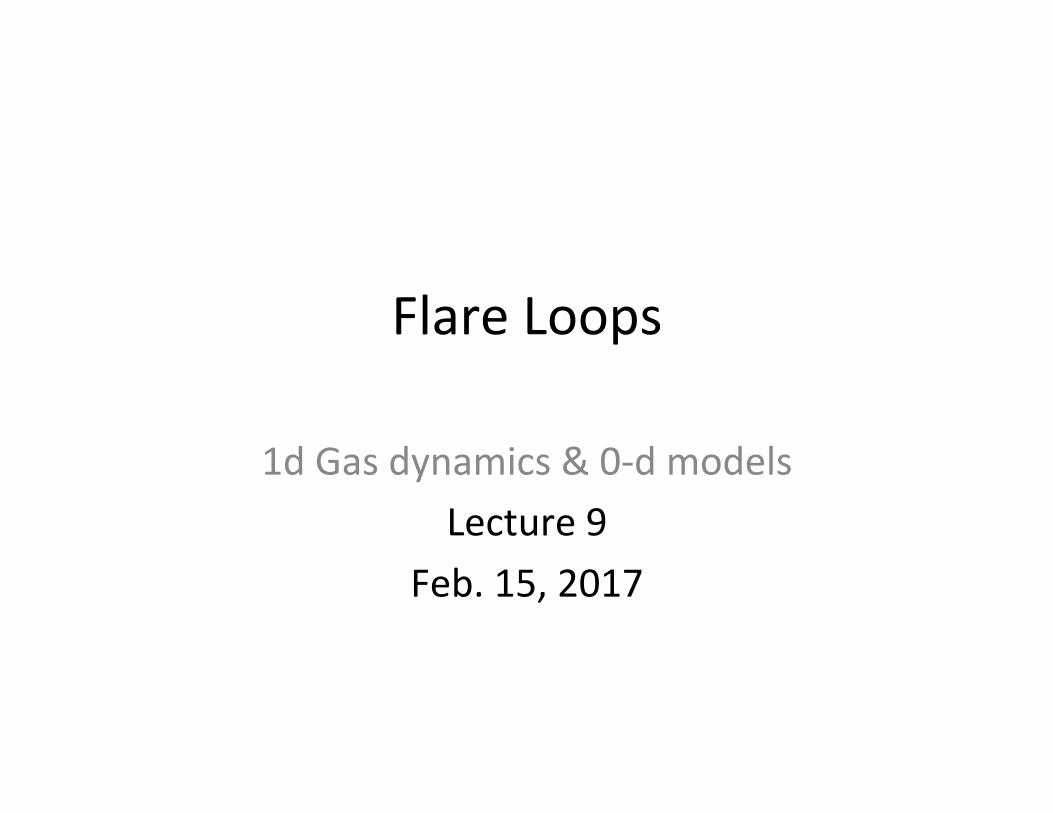
Flare Loops
1d Gas dynamics & 0-‐d models Lecture 9
Feb. 15, 2017
u A
s=0 s=L
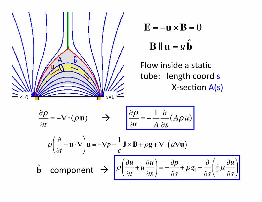
E = −u×B = 0
B ||u = u b̂b ^ Flow inside a staBc
tube: length coord s X-‐secBon A(s)
∂ρ∂t
= −∇⋅ (ρu) ∂ρ∂t
= −1A∂∂s(Aρu)
ρ∂∂t+u ⋅∇
$
%&
'
()u = −∇p+
1cJ×B+ ρg+∇⋅ µ∇u( )
ρ∂u∂t+u∂u
∂s"
#$
%
&'= −
∂p∂s+ ρg|| +
∂∂s
43 µ
∂u∂s
"
#$
%
&'component b̂
u A b ^
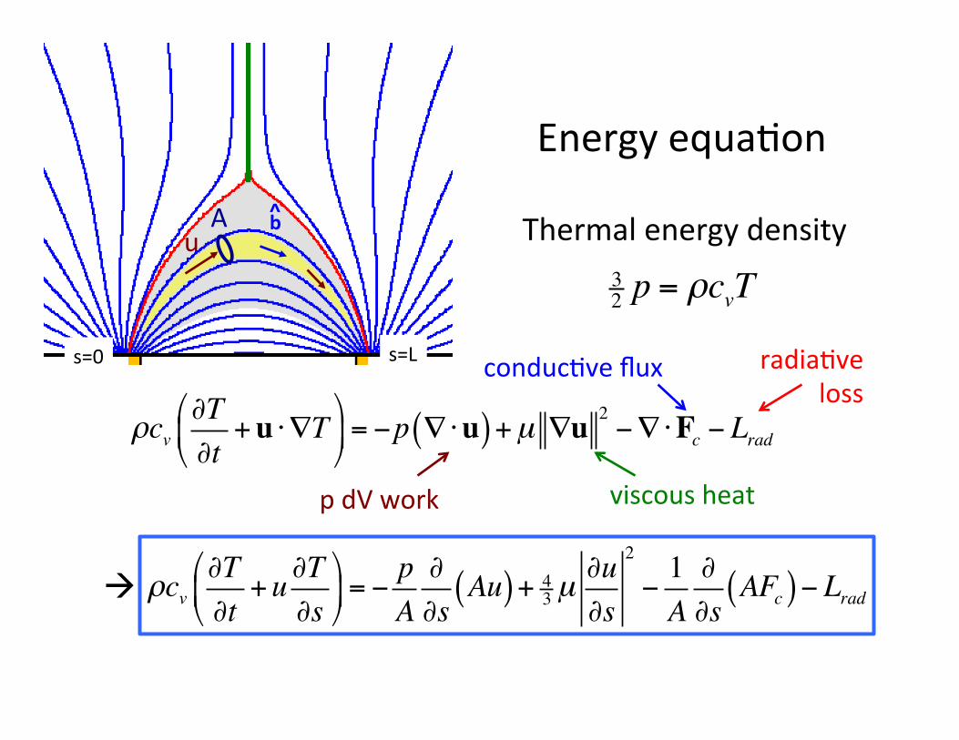
ρcv∂T∂t
+u ⋅∇T$
%&
'
()= −p ∇⋅u( )+µ ∇u 2
−∇⋅Fc − Lrad
32 p = ρcvT
Thermal energy density
ρcv∂T∂t
+u∂T∂s
"
#$
%
&'= −
pA∂∂s
Au( )+ 43 µ
∂u∂s
2
−1A∂∂s
AFc( )− Lrad
Energy equaBon
conducBve flux radiaBve loss
viscous heat p dV work
s=0 s=L
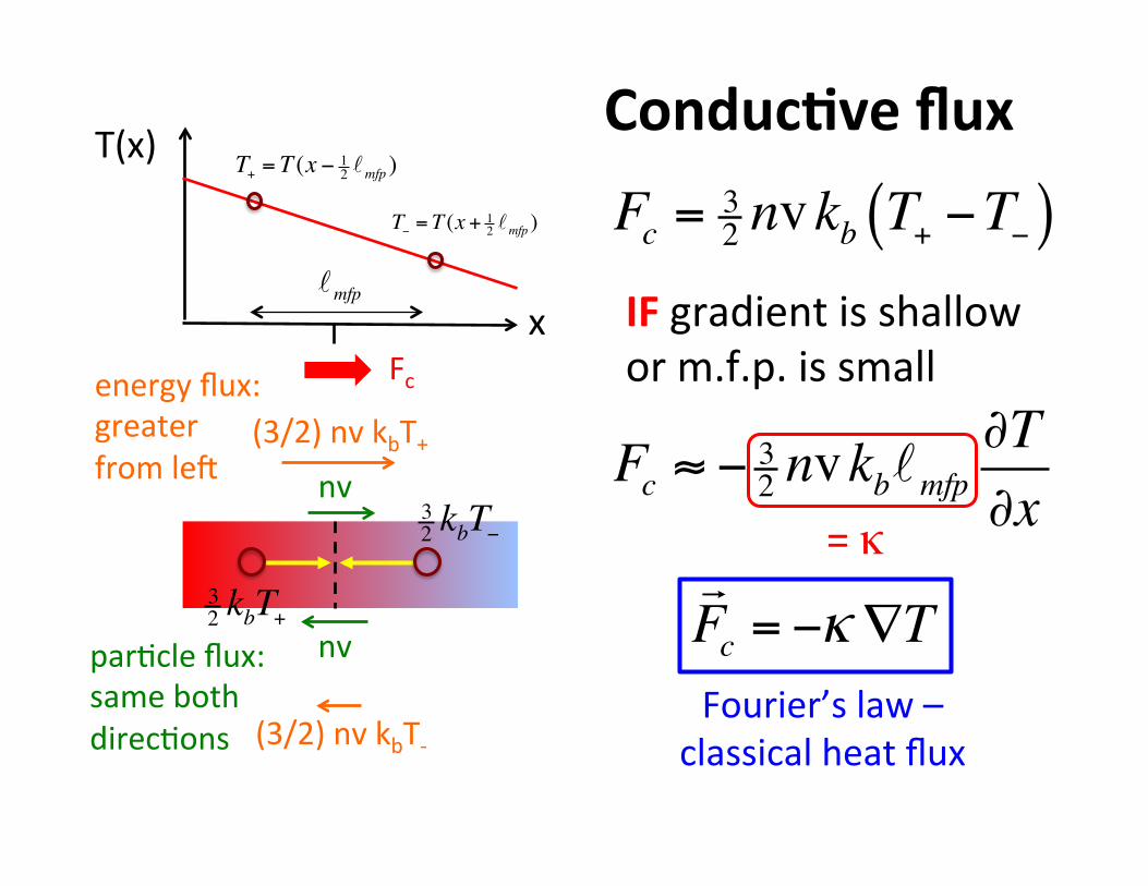
T(x)
x
nv
nv parBcle flux: same both direcBons
32 kbT+
32 kbT−
(3/2) nv kbT+
(3/2) nv kbT-‐
energy flux: greater from leU
Fc = 32 nvkb T+ −T−( )
Conduc*ve flux T− = T (x + 1
2 ℓmfp )
T+ = T (x − 12 ℓmfp )
ℓmfp
Fc ≈ − 32 nvkbℓmfp
∂T∂x
IF gradient is shallow or m.f.p. is small
!Fc = −κ∇T
= κ
Fourier’s law – classical heat flux
Fc
T(x)
x
T− = T (x + 12 ℓmfp )
T+ = T (x − 12 ℓmfp )
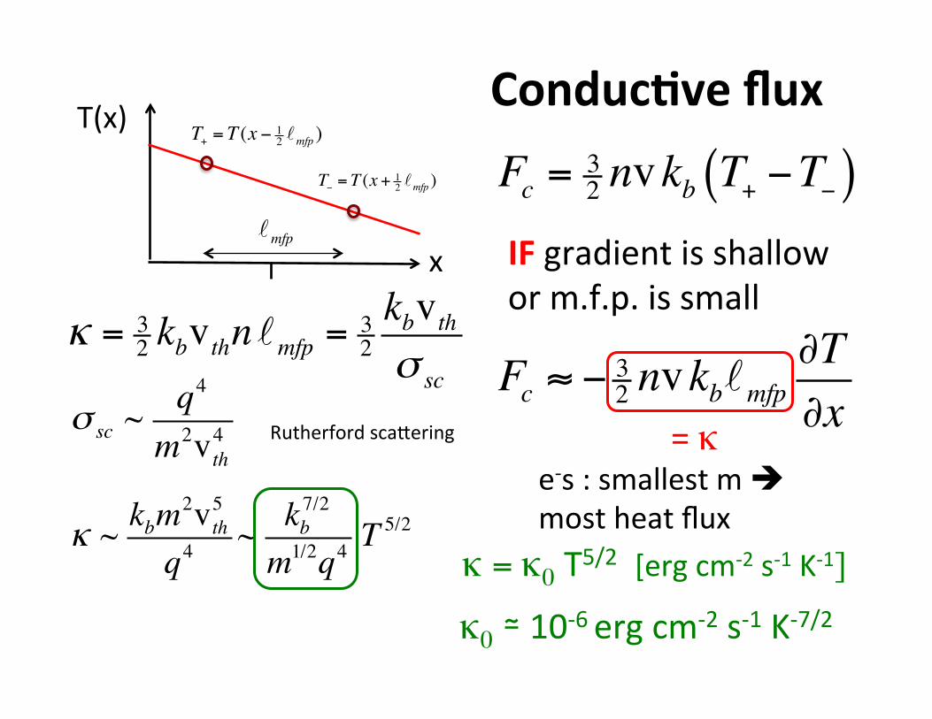
ℓmfp IF gradient is shallow or m.f.p. is small
= κ
κ = 32 kbvthnℓmfp = 3
2kbvthσ sc
σ sc ~q4
m2vth4
κ ~ kbm2vth
5
q4~ kb
7/2
m1/2q4T 5/2
e-‐s : smallest m most heat flux
κ = κ0 T5/2 [erg cm-‐2 s-‐1 K-‐1]
κ0 ≃ 10-‐6 erg cm-‐2 s-‐1 K-‐7/2
Conduc*ve flux Fc = 3
2 nvkb T+ −T−( )
Fc ≈ − 32 nvkbℓmfp
∂T∂xRutherford sca\ering
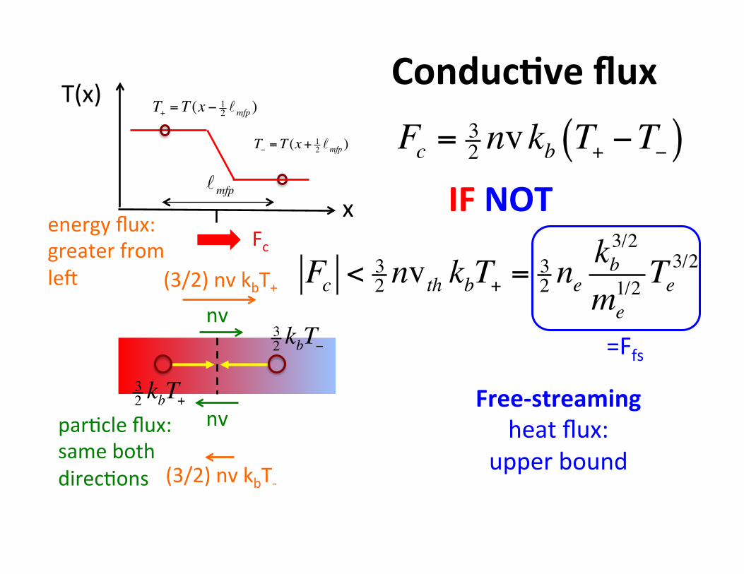
T(x)
x
nv
nv parBcle flux: same both direcBons
32 kbT+
32 kbT−
(3/2) nv kbT+
(3/2) nv kbT-‐
energy flux: greater from leU
T− = T (x + 12 ℓmfp )
T+ = T (x − 12 ℓmfp )
ℓmfp
Fc < 32 nvth kbT+ = 3
2 nekb3/2
me1/2 Te
3/2
IF NOT
Free-‐streaming heat flux:
upper bound
=Ffs
Fc
Conduc*ve flux Fc = 3
2 nvkb T+ −T−( )
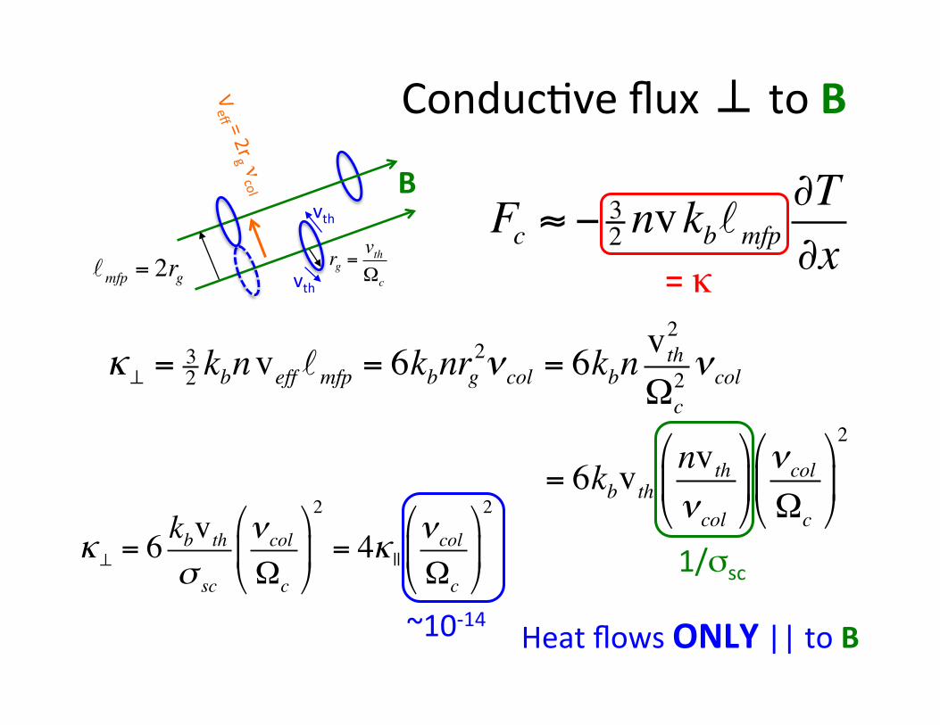
ℓmfp = 2rg
Fc ≈ − 32 nvkbℓmfp
∂T∂x= κ
κ⊥ = 32 kbnveff ℓmfp = 6kbnrg
2νcol = 6kbnvth2
Ωc2 νcol
vth
vth rg =
vthΩc
= 6kbvthnvthνcol
!
"#
$
%&νcol
Ωc
!
"#
$
%&
2
κ⊥ = 6kbvthσ sc
νcol
Ωc
#
$%
&
'(
2
= 4κ ||νcol
Ωc
#
$%
&
'(
2
1/σsc
~10-‐14
ConducBve flux ⊥ to B
B
Heat flows ONLY || to B
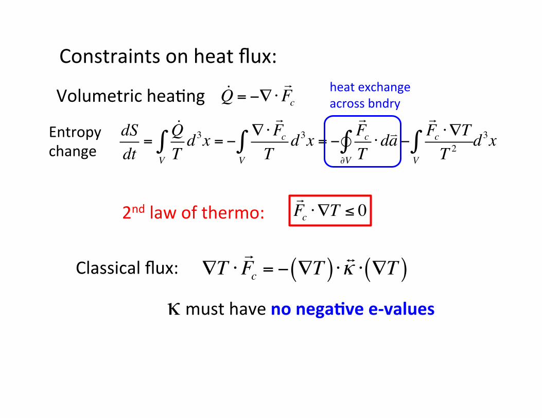
Constraints on heat flux: !Q = −∇⋅
"Fc
dSdt
=!QTd3x
V∫ = −
∇⋅"FcT
d3xV∫ = −
"FcT⋅d#a −
∂V$∫
"Fc ⋅∇TT 2
V∫ d3x
Volumetric heaBng
Entropy change
2nd law of thermo: !Fc ⋅∇T ≤ 0
heat exchange across bndry
∇T ⋅Fc = − ∇T( ) ⋅
κ ⋅ ∇T( )Classical flux:
κ must have no nega*ve e-‐values
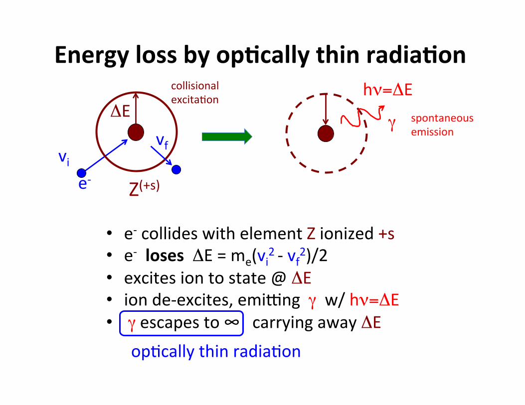
Z(+s) e-‐ vi
vf
hν=ΔE
• e-‐ collides with element Z ionized +s • e-‐ loses ΔE = me(vi2 -‐ vf2)/2 • excites ion to state @ ΔE • ion de-‐excites, emieng γ w/ hν=ΔE • γ escapes to ∞ carrying away ΔE
opBcally thin radiaBon
γ ΔE collisional excitaBon
spontaneous emission
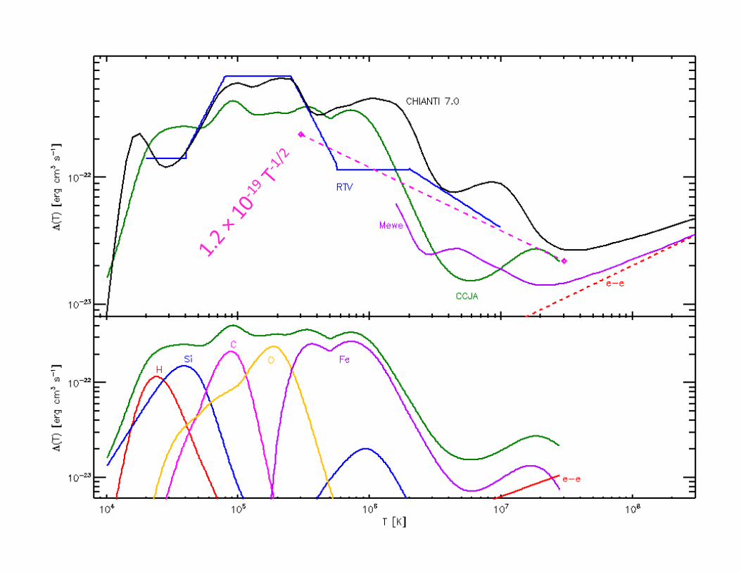
Energy loss by op*cally thin radia*on
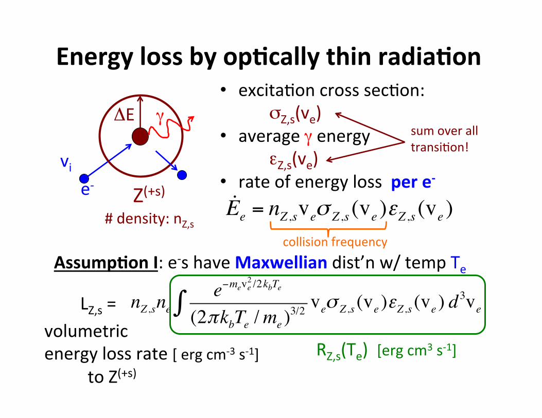
• excitaBon cross secBon: σZ,s(ve)
• average γ energy εZ,s(ve)
• rate of energy loss per e-‐
Energy loss by op*cally thin radia*on
Ee = nZ ,sveσ Z ,s (ve )εZ ,s (ve )
nZ ,snee−meve
2 /2kbTe
(2πkbTe /me )3/2 veσ Z ,s (ve )εZ ,s (ve ) d
3ve∫
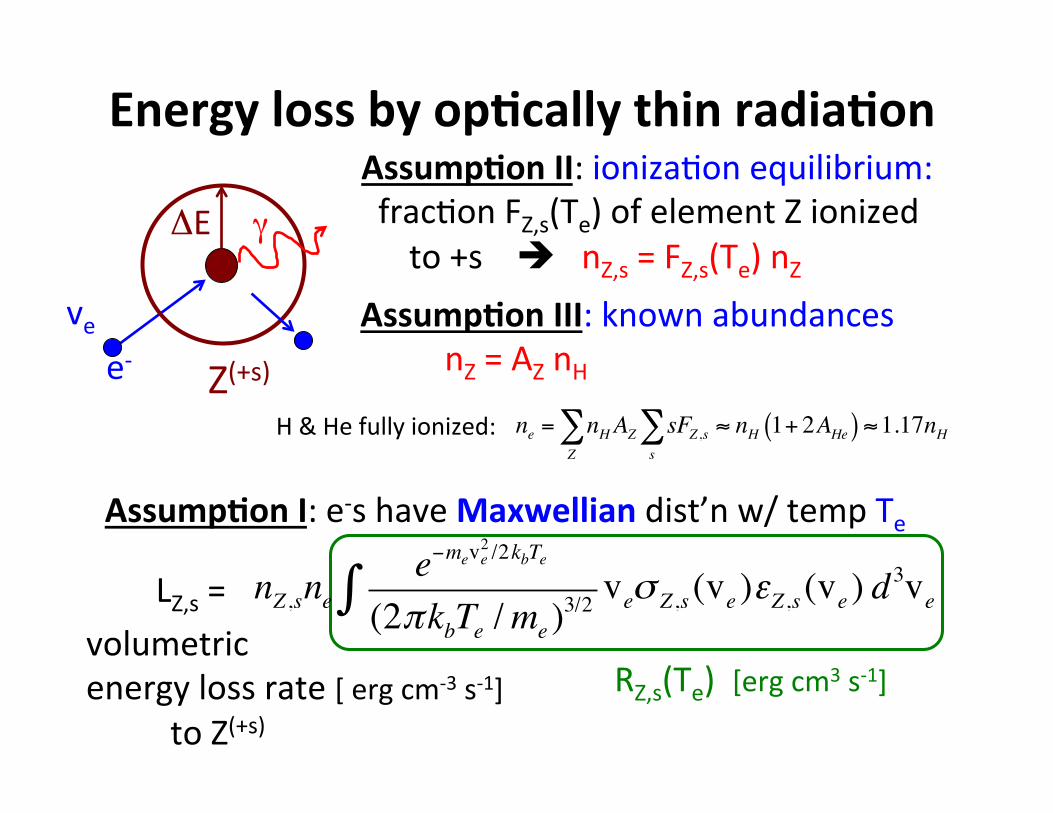
Assump*on I: e-‐s have Maxwellian dist’n w/ temp Te
RZ,s(Te) [erg cm3 s-‐1] volumetric energy loss rate [ erg cm-‐3 s-‐1] to Z(+s)
Z(+s) e-‐ vi
ΔE γ
LZ,s =
collision frequency
# density: nZ,s
sum over all transiBon!
Assump*on I: e-‐s have Maxwellian dist’n w/ temp Te
LX,s =
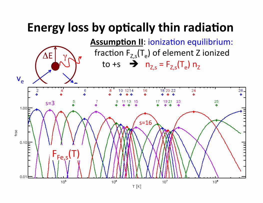
Assump*on II: ionizaBon equilibrium: fracBon FZ,s(Te) of element Z ionized
to +s nZ,s = FZ,s(Te) nZ
X(+s) e-‐ ve
ΔE γ
RX,s(Te) [erg cm3 s-‐1] volumetric energy loss rate [ erg cm-‐3 s-‐1] to X(+s)
nX,snee−meve
2 /2kbTe
(2πkbTe /me )3/2 veσ X,s (ve )εX,s (ve ) d
3ve∫
Energy loss by op*cally thin radia*on
FFe,s(T)
s=3
s=16
Assump*on I: e-‐s have Maxwellian dist’n w/ temp Te
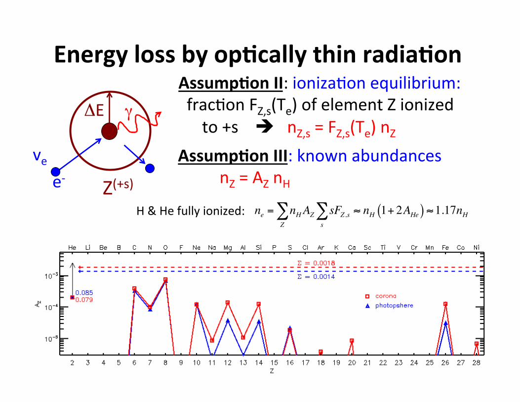
Assump*on II: ionizaBon equilibrium: fracBon FZ,s(Te) of element Z ionized
to +s nZ,s = FZ,s(Te) nZ
Z(+s) e-‐ ve
ΔE γ
Assump*on III: known abundances nZ = AZ nH
ne = nHAZ sFZ ,s ≈ nH 1+ 2AHe( )s∑
Z∑ ≈1.17nHH & He fully ionized:
Energy loss by op*cally thin radia*on
nZ ,snee−meve
2 /2kbTe
(2πkbTe /me )3/2 veσ Z ,s (ve )εZ ,s (ve ) d
3ve∫
RZ,s(Te) [erg cm3 s-‐1] volumetric energy loss rate [ erg cm-‐3 s-‐1] to Z(+s)
LZ,s =
Assump*on I: e-‐s have Maxwellian dist’n w/ temp Te
Assump*on II: ionizaBon equilibrium: fracBon FZ,s(Te) of element Z ionized
to +s nZ,s = FZ,s(Te) nZ
Z(+s) e-‐ ve
ΔE γ
Assump*on III: known abundances nZ = AZ nH
ne = nHAZ sFZ ,s ≈ nH 1+ 2AHe( )s∑
Z∑ ≈1.17nHH & He fully ionized:
Energy loss by op*cally thin radia*on
nZ ,snee−meve
2 /2kbTe
(2πkbTe /me )3/2 veσ Z ,s (ve )εZ ,s (ve ) d
3ve∫
RZ,s(Te) [erg cm3 s-‐1] volumetric energy loss rate [ erg cm-‐3 s-‐1] to Z(+s)
LZ,s =
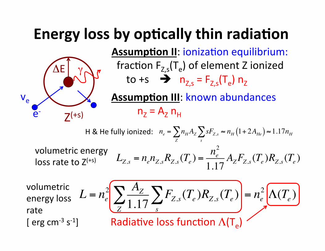
volumetric energy loss rate to Z(+s)
Assump*on II: ionizaBon equilibrium: fracBon FZ,s(Te) of element Z ionized
to +s nZ,s = FZ,s(Te) nZ
Z(+s) e-‐ ve
ΔE γ
Assump*on III: known abundances nZ = AZ nH
H & He fully ionized:
LZ ,s = nenZ ,sRZ ,s (Te ) =ne2
1.17AZFZ ,s (Te )RZ ,s (Te )
L = ne2 AZ
1.17FZ ,s (Te )RZ ,s (Te )
s∑
Z∑ = ne
2 Λ(Te )volumetric energy loss rate [ erg cm-‐3 s-‐1] RadiaBve loss funcBon Λ(Te)
Energy loss by op*cally thin radia*on
ne = nHAZ sFZ ,s ≈ nH 1+ 2AHe( )s∑
Z∑ ≈1.17nH
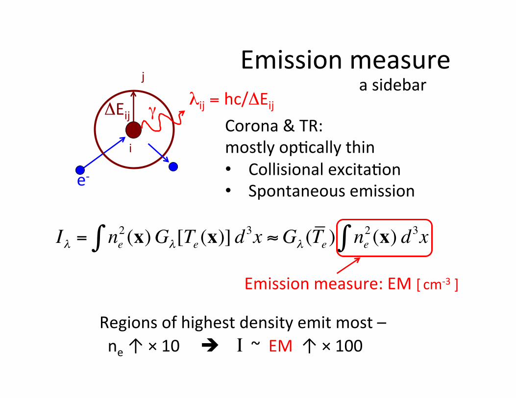
Emission measure
e-‐
ΔEij γ λij = hc/ΔEij j
i
Corona & TR: mostly opBcally thin • Collisional excitaBon • Spontaneous emission
Iλ = ne2 (x)Gλ[Te(x)]∫ d3x ≈Gλ (Te ) ne
2 (x)∫ d3x
Emission measure: EM [ cm-‐3 ]
Regions of highest density emit most – ne ↑ × 10 I ~ EM ↑ × 100
a sidebar
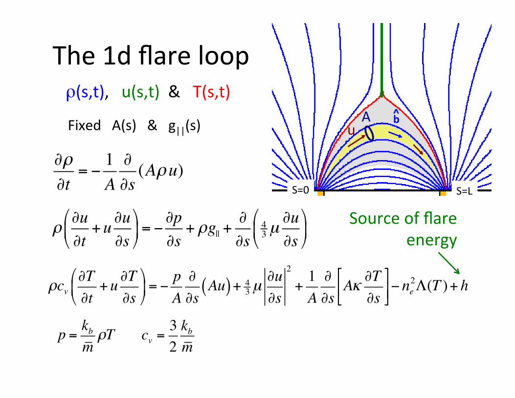
The 1d flare loop
u A b ^
∂ρ∂t
= −1A∂∂s(Aρu)
ρ∂u∂t+u∂u
∂s"
#$
%
&'= −
∂p∂s+ ρg|| +
∂∂s
43 µ
∂u∂s
"
#$
%
&'
ρ(s,t), u(s,t) & T(s,t)
Fixed A(s) & g||(s)
p = kbmρT cv =
32kbm
Source of flare energy
S=L S=0
ρcv∂T∂t
+u∂T∂s
"
#$
%
&'= −
pA∂∂s
Au( )+ 43 µ
∂u∂s
2
+1A∂∂s
Aκ ∂T∂s
)
*+,
-.− ne
2Λ(T )+ h
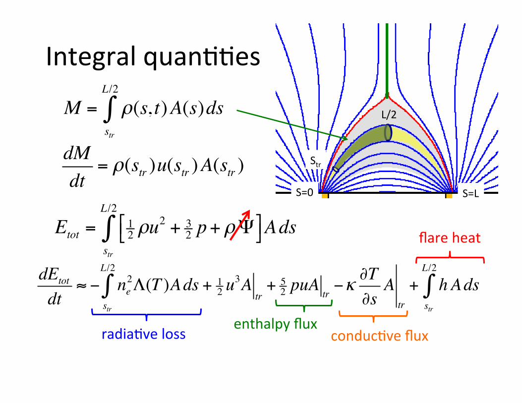
Integral quanBBes
Str
S=L
M = ρ(s, t)A(s)dsstr
L/2
∫ L/2
S=0
dMdt
= ρ(str )u(str )A(str )
Etot = 12 ρu
2 + 32 p+ ρΨ"# $%Ads
str
L/2
∫
dEtot
dt≈ − ne
2Λ(T )Adsstr
L/2
∫ + 12 u
3Atr+ 52 puA tr
−κ∂T∂s
Atr
+ hAdsstr
L/2
∫enthalpy flux
radiaBve loss conducBve flux
flare heat
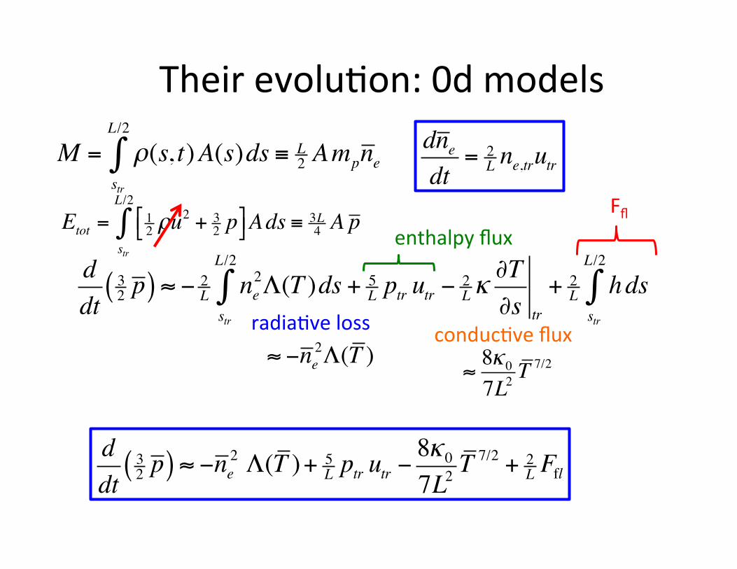
Their evoluBon: 0d models
M = ρ(s, t)A(s)dsstr
L/2
∫ ≡ L2 Ampne
dnedt
= 2L ne,trutr
Etot = 12 ρu
2 + 32 p!" #$Ads ≡ 3L
4 A pstr
L/2
∫ enthalpy flux
radiaBve loss conducBve flux
Ffl
ddt
32 p( ) ≈ − 2
L ne2Λ(T )ds
str
L/2
∫ + 5L ptr utr − 2
Lκ∂T∂s tr
+ 2L hdsstr
L/2
∫
≈ −ne2Λ(T )
≈8κ07L2
T 7/2
ddt
32 p( ) ≈ −ne2 Λ(T )+ 5
L ptr utr −8κ07L2
T 7/2 + 2L Ffl
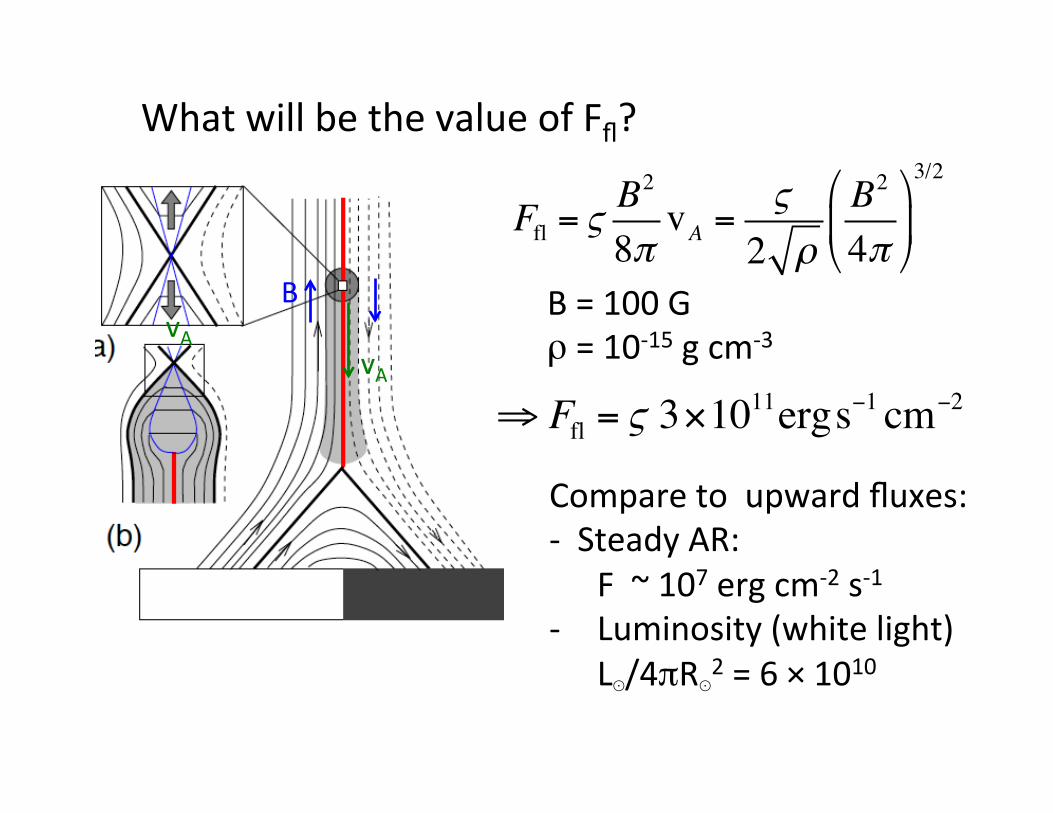
What will be the value of Ffl?
vA vA
B
Ffl = ςB2
8πvA =
ς2 ρ
B2
4π!
"#
$
%&
3/2
B = 100 G ρ = 10-‐15 g cm-‐3
⇒ Ffl = ς 3×10¹¹ergs−1 cm−2
Compare to upward fluxes: -‐ Steady AR:
F ~ 107 erg cm-‐2 s-‐1 -‐ Luminosity (white light)
L⊙/4πR⊙2 = 6 × 10¹⁰
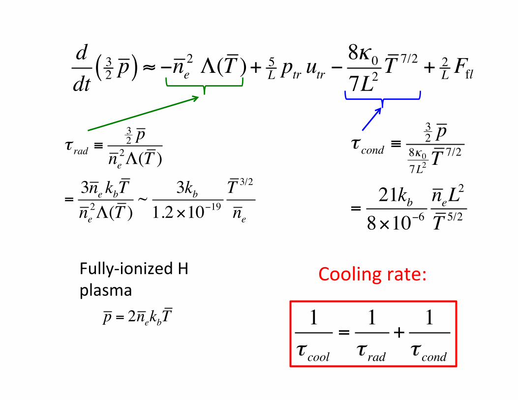
τ rad ≡32 p
ne2Λ(T )
=3ne kbTne2Λ(T )
~ 3kb1.2×10−19
T 3/2
ne
ddt
32 p( ) ≈ −ne2 Λ(T )+ 5
L ptr utr −8κ07L2
T 7/2 + 2L Ffl
τ cond ≡32 p
8κ07L2T 7/2
=21kb8×10−6
neL2
T 5/2
1τ cool
=1τ rad
+1
τ cond
Cooling rate:
p = 2nekbT
Fully-‐ionized H plasma
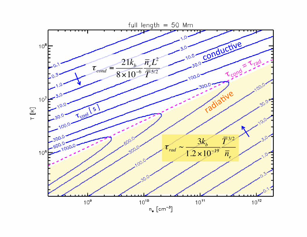
τ rad ~3kb
1.2×10⁻¹⁹T 3/2
ne
τ cond =21kb8×10−6
neL2
T 5/2
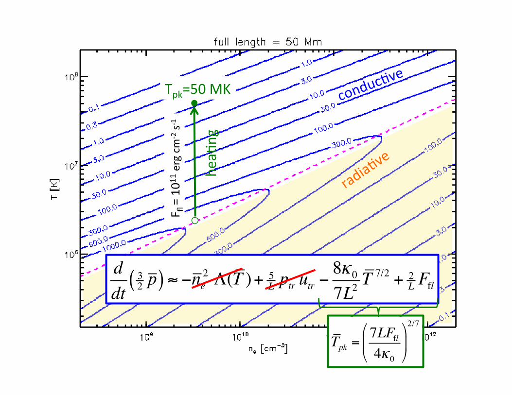
ddt
32 p( ) ≈ −ne2 Λ(T )+ 5
L ptr utr −8κ07L2
T 7/2 + 2L Ffl
Tpk =7LFfl4κ0
!
"#
$
%&
2/7
Tpk=50 MK
F fl = 101
1 erg cm
-‐2 s-‐
1
heaB
ng
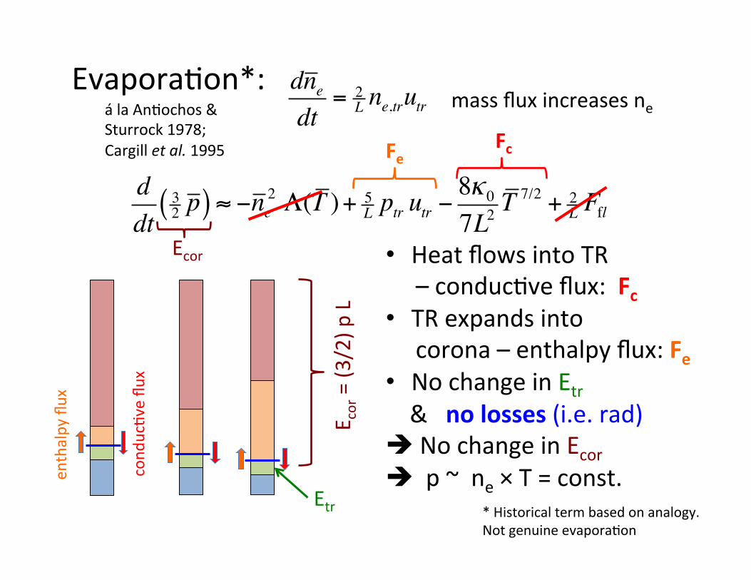
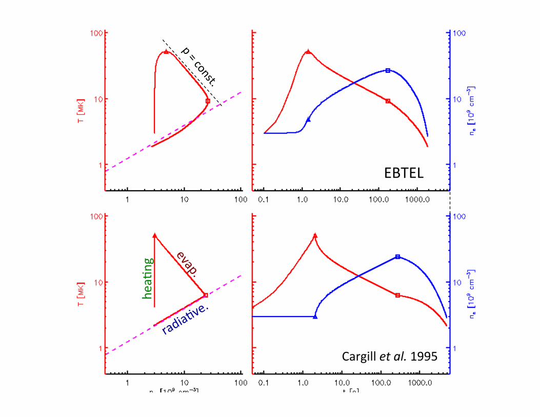
EvaporaBon*: dnedt
= 2L ne,trutr
ddt
32 p( ) ≈ −ne2 Λ(T )+ 5
L ptr utr −8κ07L2
T 7/2 + 2L Ffl
mass flux increases ne
enthalpy flux
cond
ucBve flu
x
E cor = (3
/2) p
L
Etr
• Heat flows into TR – conducBve flux: Fc • TR expands into corona – enthalpy flux: Fe • No change in Etr & no losses (i.e. rad) No change in Ecor p ~ ne × T = const.
á la AnBochos & Sturrock 1978; Cargill et al. 1995 Fe
Fc
Ecor
* Historical term based on analogy. Not genuine evaporaBon
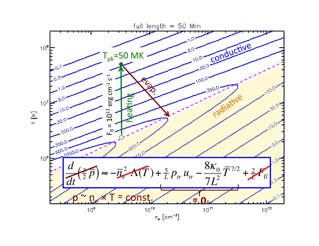
ddt
32 p( ) ≈ −ne2 Λ(T )+ 5
L ptr utr −8κ07L2
T 7/2 + 2L Ffl
≃ 0 p ~ ne × T ≃ const.
Tpk=50 MK
F fl = 101
1 erg cm
-‐2 s-‐
1
heaB
ng
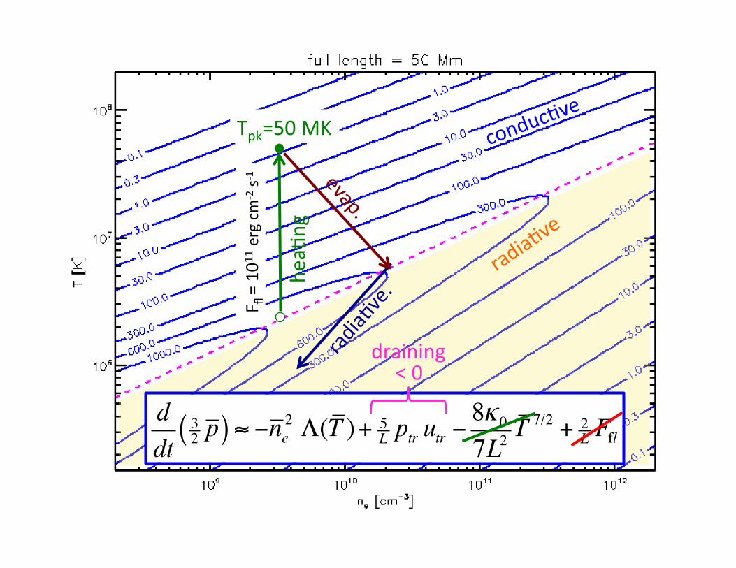
ddt
32 p( ) ≈ −ne2 Λ(T )+ 5
L ptr utr −8κ07L2
T 7/2 + 2L Ffl
draining < 0
Tpk=50 MK
F fl = 101
1 erg cm
-‐2 s-‐
1
heaB
ng
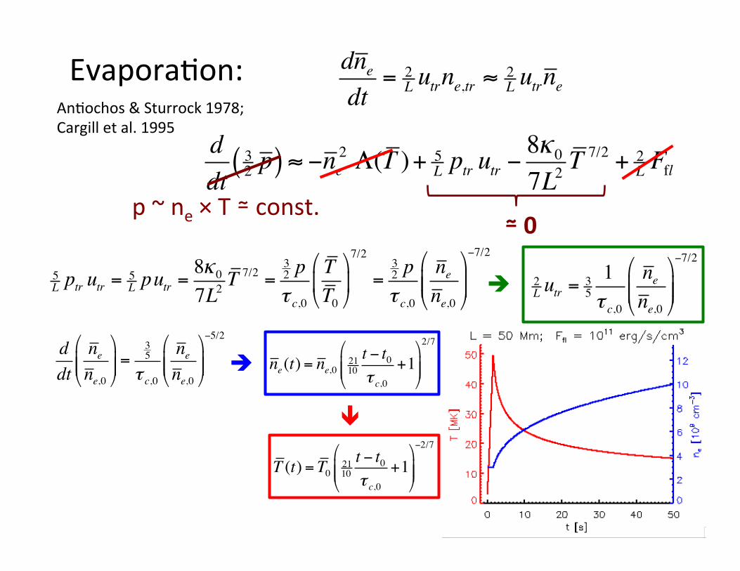
EvaporaBon: dnedt
= 2L utrne,tr ≈ 2
L utrne
ddt
32 p( ) ≈ −ne2 Λ(T )+ 5
L ptr utr −8κ07L2
T 7/2 + 2L Ffl
AnBochos & Sturrock 1978; Cargill et al. 1995
≃ 0 p ~ ne × T ≃ const.
5L ptr utr = 5
L putr =8κ07L2
T 7/2 =32 pτ c,0
TT0
!
"#
$
%&
7/2
=32 pτ c,0
nene,0
!
"##
$
%&&
−7/2
2L utr = 3
51τ c,0
nene,0
!
"##
$
%&&
−7/2
ddt
nene,0
!
"##
$
%&&=
35
τ c,0
nene,0
!
"##
$
%&&
−5/2
ne(t) = ne,0 2110t − t0τ c,0
+1"
#$$
%
&''
2/7
T (t) = T0 2110t − t0τ c,0
+1"
#$$
%
&''
−2/7
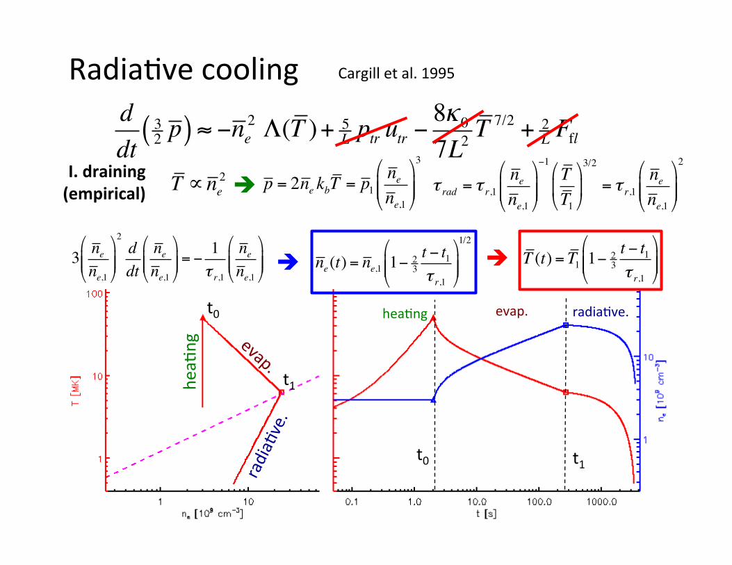
RadiaBve cooling ddt
32 p( ) ≈ −ne2 Λ(T )+ 5
L ptr utr −8κ07L2
T 7/2 + 2L Ffl
Cargill et al. 1995
ne(t) = ne,1 1− 23t − t1τ r,1
"
#$$
%
&''
1/2
T ∝ne2 p = 2ne kbT = p1
nene,1
!
"##
$
%&&
3
3 nene,1
!
"##
$
%&&
2ddt
nene,1
!
"##
$
%&&= −
1τ r,1
nene,1
!
"##
$
%&& T (t) = T1 1− 2
3t − t1τ r,1
"
#$$
%
&''
I. draining (empirical)
heaB
ng
radiaBve. evap. heaBng
t0 t1
t0
t1
τ rad = τ r,1nene,1
!
"##
$
%&&
−1TT1
!
"#
$
%&
3/2
= τ r,1nene,1
!
"##
$
%&&
2
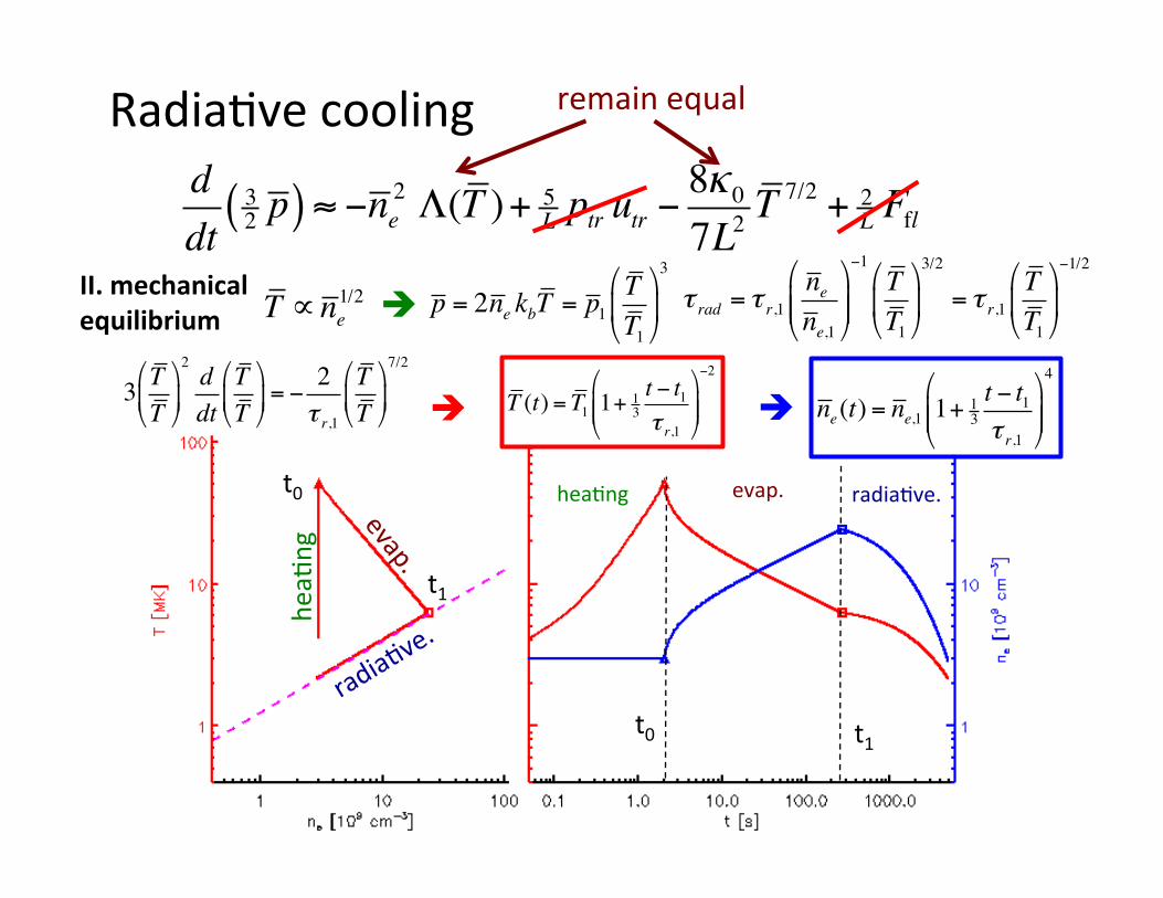
RadiaBve cooling ddt
32 p( ) ≈ −ne2 Λ(T )+ 5
L ptr utr −8κ07L2
T 7/2 + 2L Ffl
ne(t) = ne,1 1+ 13t − t1τ r,1
"
#$$
%
&''
4
T ∝ne1/2 p = 2ne kbT = p1
TT1
!
"#
$
%&
3
3 TT!
"#
$
%&
2ddt
TT!
"#
$
%&= −
2τ r,1
TT!
"#
$
%&
7/2
T (t) = T1 1+ 13t − t1τ r,1
"
#$$
%
&''
−2
II. mechanical equilibrium
heaB
ng
radiaBve. evap. heaBng
t0 t1
t0
t1
τ rad = τ r,1nene,1
!
"##
$
%&&
−1TT1
!
"#
$
%&
3/2
= τ r,1TT1
!
"#
$
%&
−1/2
remain equal
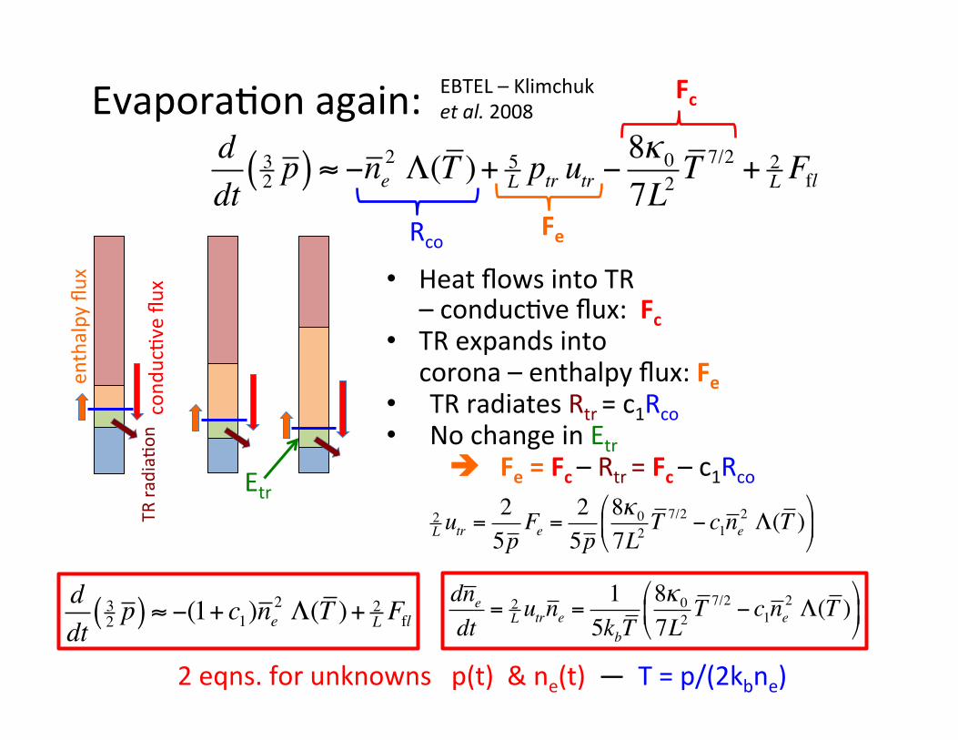
EvaporaBon again: ddt
32 p( ) ≈ −ne2 Λ(T )+ 5
L ptr utr −8κ07L2
T 7/2 + 2L Ffl
enthalpy flux
cond
ucBve flu
x
Etr
• Heat flows into TR – conducBve flux: Fc • TR expands into corona – enthalpy flux: Fe • TR radiates Rtr = c1Rco • No change in Etr
è Fe = Fc – Rtr = Fc – c1Rco
EBTEL – Klimchuk et al. 2008
Fe
Fc
Rco
ddt
32 p( ) ≈ −(1+ c1)ne2 Λ(T )+ 2
L Ffl
TR ra
diaB
on
2L utr =
25p
Fe =25p
8κ07L2
T 7/2 − c1ne2 Λ(T )
#
$%
&
'(
dnedt
= 2L utrne =
15kbT
8κ07L2
T 7/2 − c1ne2 Λ(T )
#
$%
&
'(
2 eqns. for unknowns p(t) & ne(t) — T = p/(2kbne)
EBTEL
heaB
ng
Cargill et al. 1995
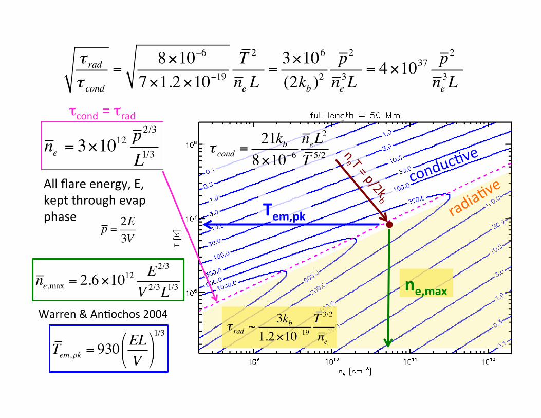
τ rad ~3kb
1.2×10⁻¹⁹T 3/2
ne
τ cond =21kb8×10−6
neL2
T 5/2
τcond = τrad
τ radτ cond
=8×10⁻⁶
7×1.2×10−19T 2
ne L=3×10⁶
(2kb )2p2
ne3L
= 4×1037 p2
ne3L
ne = 3×10¹² p2/3
L1/3
ne,max = 2.6×10¹² E 2/3
V 2/3L1/3
Warren & AnBochos 2004
p = 2E3V
ne,max
Tem,pk All flare energy, E, kept through evap phase
Tem,pk = 930ELV
!
"#
$
%&1/3
Tpk =7LFfl4κ0
!
"#
$
%&
2/7
= 5×10⁷K
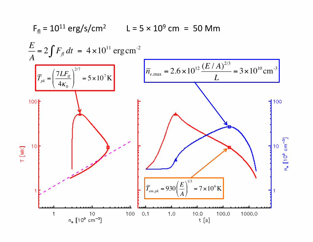
L = 5 × 109 cm = 50 Mm Ffl = 1011 erg/s/cm2
EA= 2 Ffl dt∫ = 4×10¹¹ ergcm-2
Tem,pk = 930EA!
"#
$
%&1/3
= 7×10⁶K
ne,max = 2.6×10¹² (E / A)2/3
L= 3×1010cm-3
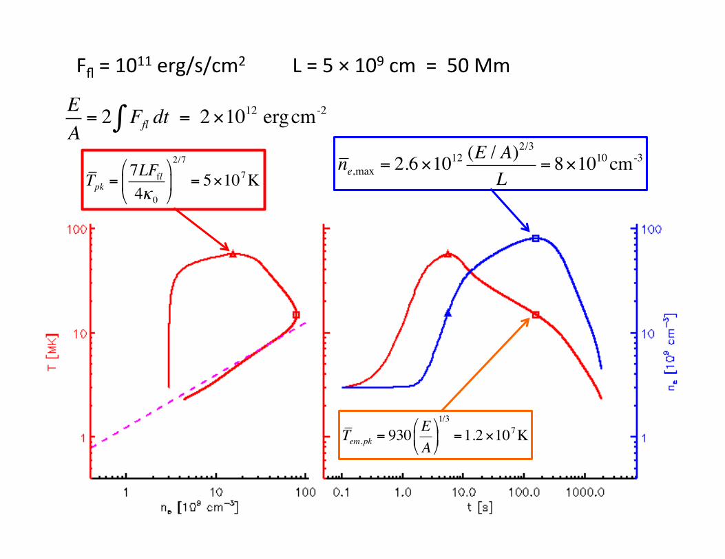
ne,max = 2.6×10¹² (E / A)2/3
L= 8×1010cm-3
Tpk =7LFfl4κ0
!
"#
$
%&
2/7
= 5×10⁷K
Ffl = 1011 erg/s/cm2
EA= 2 Ffl dt∫ = 2×10¹² ergcm-2
Tem,pk = 930EA!
"#
$
%&1/3
=1.2×10⁷K
L = 5 × 109 cm = 50 Mm
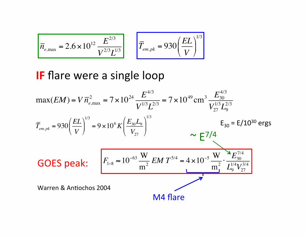
ne,max = 2.6×10¹² E 2/3
V 2/3L1/3
Warren & AnBochos 2004
Tem,pk = 930ELV
!
"#
$
%&1/3
IF flare were a single loop
max(EM ) =V ne,max2 = 7×1024 E 4/3
V 1/3L2/3= 7×1049cm3 E30
4/3
V271/3L9
2/3
Tem,pk = 930ELV
!
"#
$
%&1/3
= 9×10⁶K E30L9V27
!
"#
$
%&
1/3
F1−8 ≈10−63 Wm2 EM T 5/4 = 4×10⁻⁵ W
m2 ⋅E307/4
L91/4V27
3/4GOES peak:
E30 = E/1030 ergs
M4 flare
~ E7/4
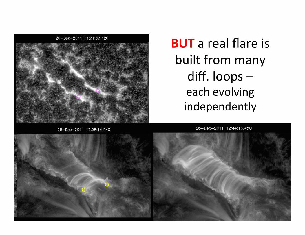
BUT a real flare is built from many diff. loops – each evolving independently
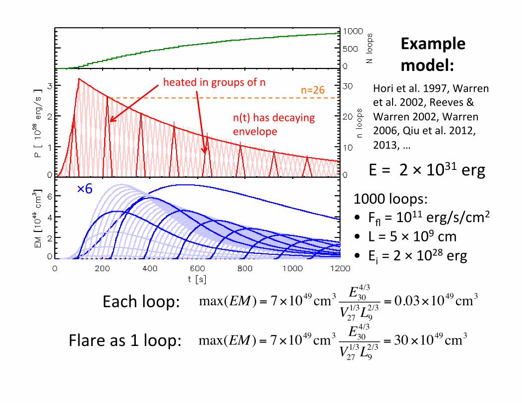
1000 loops: • Ffl = 1011 erg/s/cm2
• L = 5 × 109 cm • Ei = 2 × 1028 erg
max(EM ) = 7×1049cm3 E304/3
V271/3L9
2/3 = 0.03×1049cm3
×6
max(EM ) = 7×1049cm3 E304/3
V271/3L9
2/3 = 30×1049cm3
Each loop:
Flare as 1 loop:
Example model:
heated in groups of n
n(t) has decaying envelope
n=26 Hori et al. 1997, Warren et al. 2002, Reeves & Warren 2002, Warren 2006, Qiu et al. 2012, 2013, …
E = 2 × 1031 erg
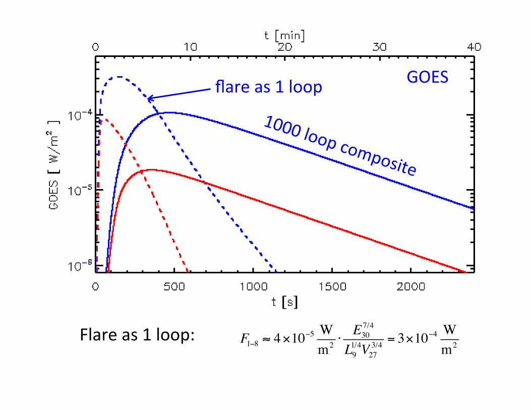
GOES
F1−8 ≈ 4×10⁻⁵ Wm2 ⋅
E307/4
L91/4V27
3/4 = 3×10⁻⁴ Wm2
Flare as 1 loop:
flare as 1 loop
1000 loop composite
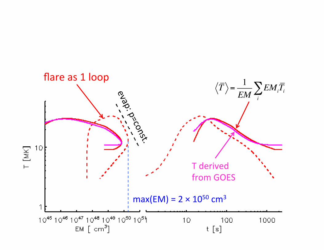
T =1EM
EMii∑ Ti
T derived from GOES
flare as 1 loop
max(EM) = 2 × 1050 cm3
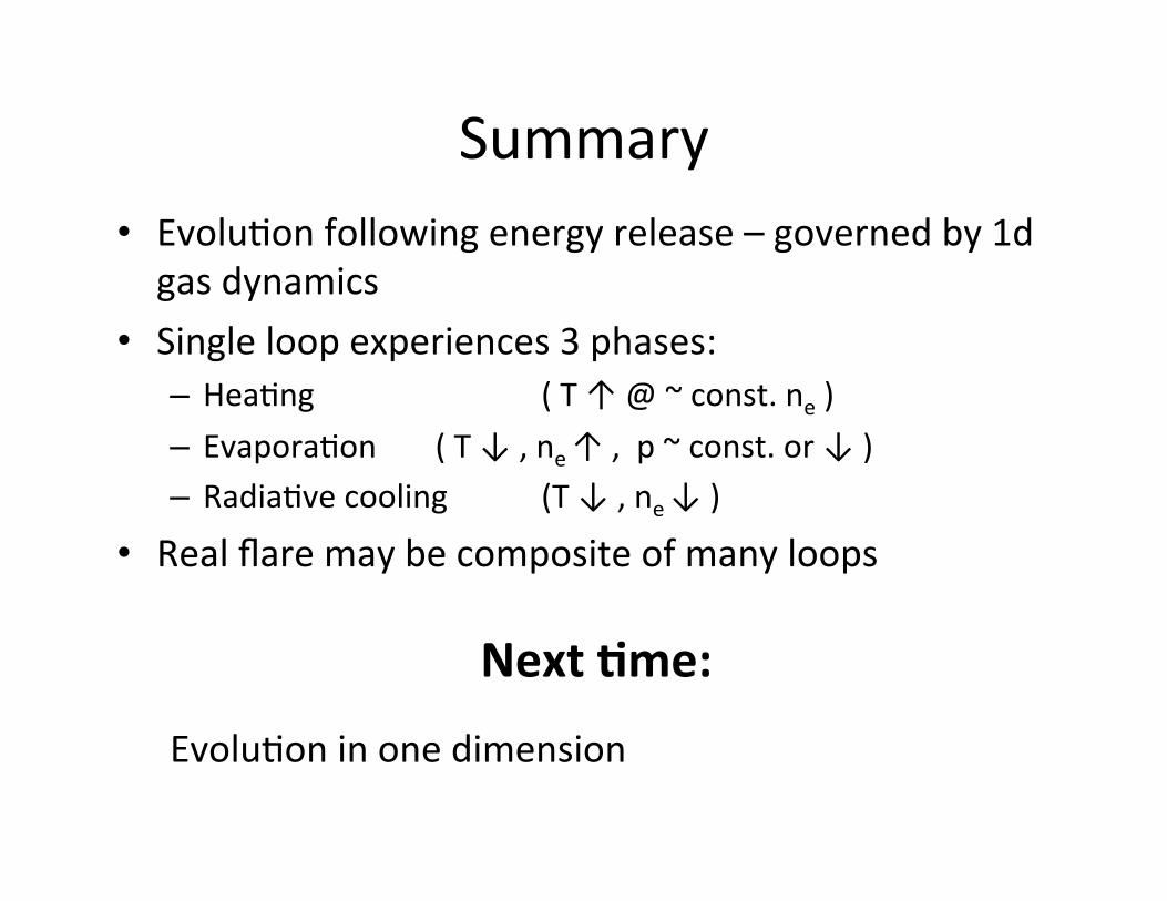
Summary • EvoluBon following energy release – governed by 1d gas dynamics
• Single loop experiences 3 phases: – HeaBng ( T ↑ @ ~ const. ne ) – EvaporaBon ( T ↓ , ne ↑ , p ~ const. or ↓ ) – RadiaBve cooling (T ↓ , ne ↓ )
• Real flare may be composite of many loops
Next *me:
EvoluBon in one dimension