From Pattern Formation to Phase Field Crystal Model

吳國安 (Kuo-An Wu)

清華大學物理系Department of Physics

National Tsing Hua University

3/23/2011

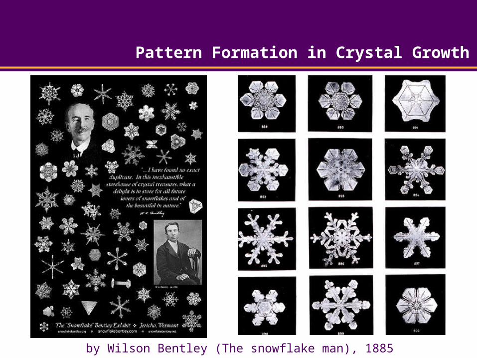
Pattern Formation in Crystal Growth

by Wilson Bentley (The snowflake man), 1885

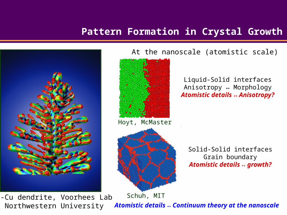
Pattern Formation in Crystal Growth

Al-Cu dendrite, Voorhees Lab Northwestern University

At the nanoscale (atomistic scale)

Liquid-Solid interfacesAnisotropy ↔ Morphology

Atomistic details ↔ Anisotropy?

Solid-Solid interfacesGrain boundary

Atomistic details ↔ growth?

Atomistic details ↔ Continuum theory at the nanoscale

Hoyt, McMaster

Schuh, MIT

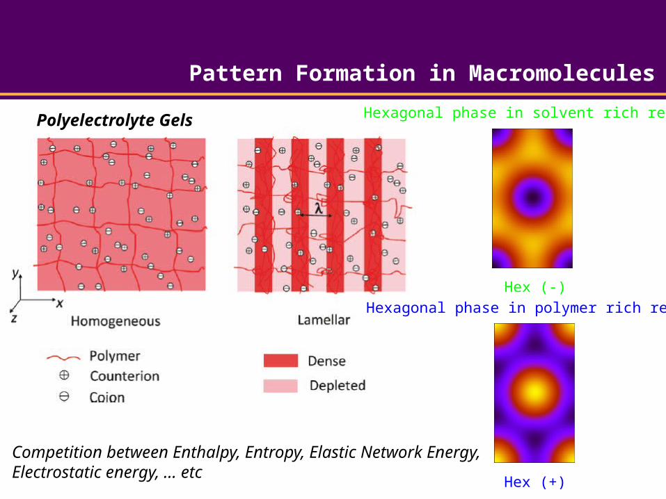
Pattern Formation in Macromolecules

Polyelectrolyte Gels

Hex (-)

Hexagonal phase in solvent rich region

Hex (+)

Hexagonal phase in polymer rich region

Competition between Enthalpy, Entropy, Elastic Network Energy,Electrostatic energy, … etc

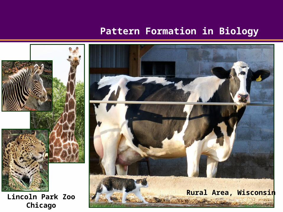
Pattern Formation in Biology

Lincoln Park ZooChicago

Rural Area, Wisconsin

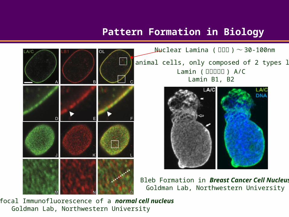
Pattern Formation in Biology

Bleb Formation in Breast Cancer Cell NucleusGoldman Lab, Northwestern University

Confocal Immunofluorescence of a normal cell nucleusGoldman Lab, Northwestern University

Lamin ( 核纖層蛋白 ) A/CLamin B1, B2

Nuclear Lamina ( 核纖層 ) ～ 30-100nm

In animal cells, only composed of 2 types lamins

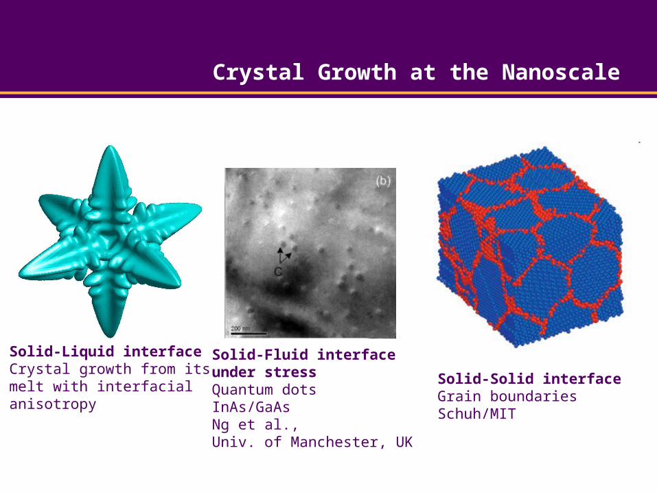
Crystal Growth at the Nanoscale

Solid-Solid interfaceGrain boundariesSchuh/MIT

Solid-Liquid interfaceCrystal growth from its melt with interfacial anisotropy

Solid-Fluid interface under stressQuantum dots InAs/GaAsNg et al., Univ. of Manchester, UK

2

t

n n nsolid liquid

T D T

LV cD T T

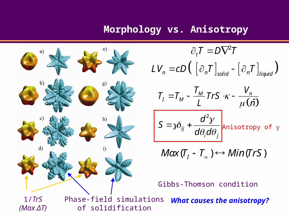
Gibbs-Thomson condition

2

ˆnM

I M

iji j

VTT T TrS

L n

dS

d d

1/TrS(Max ΔT)

Phase-field simulationsof solidification

( ) ( )IMax T T Min TrS

Morphology vs. Anisotropy

Anisotropy of g

What causes the anisotropy?

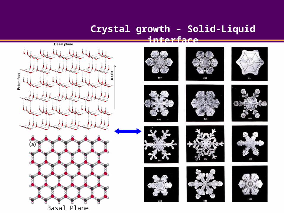
Basal Plane

Crystal growth – Solid-Liquid interface

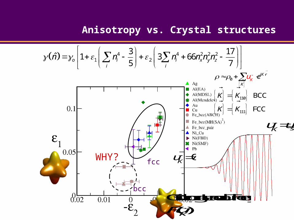
4 4 2 2 21 2

3 17ˆ 1 3 66

5 7o i i x y zi i

n n n n n n

Anisotropy vs. Crystal structures

fcc

bcc

WHY?

0

110

111

BCC

FCC

iK r

KKe

K

K

u

K

K

sKu u

0Ku

Ginzburg-Landau Theory

( )k

F u

DF

u110

2 3 42 110 3 110 4 110F a u a u a u

g

Liquid Solid

2 3 0,, , ,

0,

20

4 0,, , ,

2

i j k

i j k l

i jij ijk i j k K K K

i j i j kB

ijkl i j k l iK K K Ki j k l i

i j K

i

Ka c a c u u u

n k TF dr

a c u u u u b

u

cu z

z

u

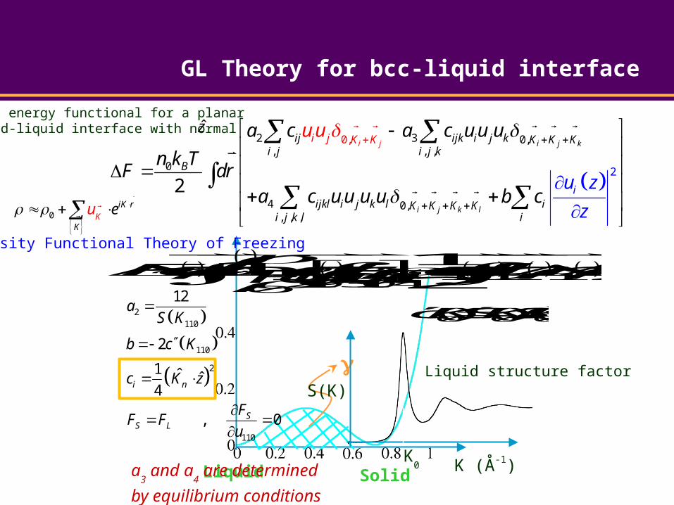
GL Theory for bcc-liquid interface

2110

110

2

110

12

2

1 ˆ ˆ4

, 0

i n

SS L

aS K

b c K

c K z

FF F

u

S(K)

K (Å-1)K

0

20 0 0( ) ( ) / ( )c K S K S K

a3 and a

4 are determined

by equilibrium conditions

Liquid structure factor

Density Functional Theory of Freezing

0 1 2 1 2 1 20

1ln ,

2

rF dr r dr r drdr c r r r r

0 K

iK r

K

eu

Free energy functional for a planarsolid-liquid interface with normal z

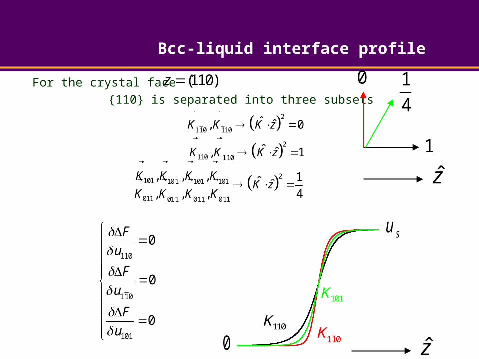
(110)z

110

110

101

0

0

0

F

u

F

u

F

u

2

110 110

2

110 110

2101 101 101 101

011 011 011 011

ˆ ˆ, 0

ˆ ˆ, 1

, , , 1ˆ ˆ4, , ,

K K K z

K K K z

K K K KK z

K K K K

110K

110K

101K

su

0 z

For the crystal face

{110} is separated into three subsets

z

1

0 1

4

Bcc-liquid interface profile

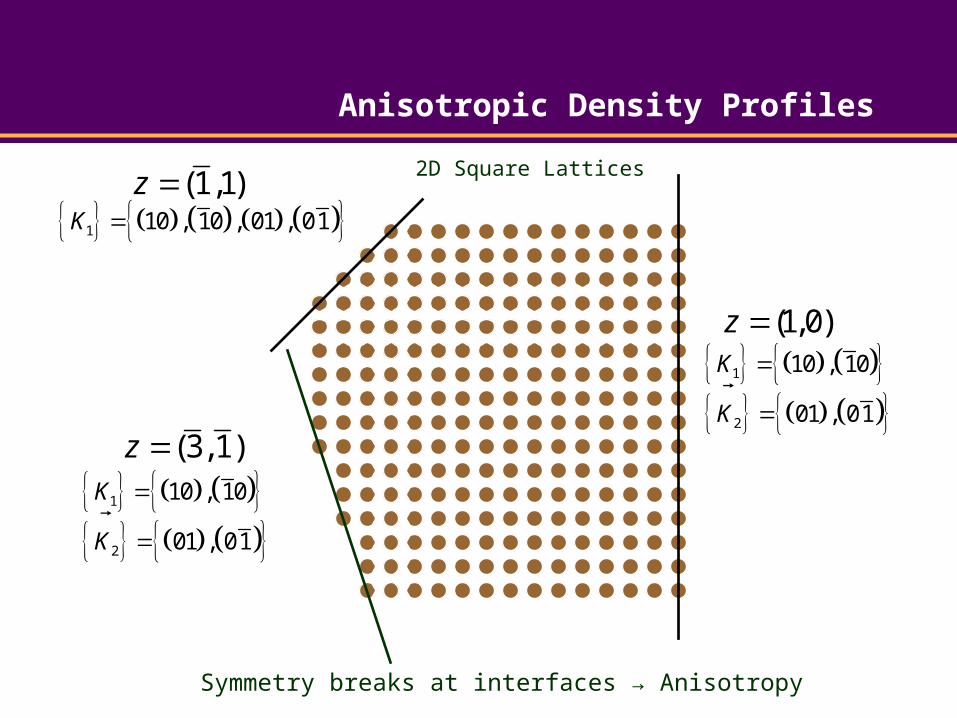
Anisotropic Density Profiles

(1,0)z

(1,1)z

1

2

10 , 10

01 , 01

K

K

1 10 , 10 , 01 , 01K

Symmetry breaks at interfaces → Anisotropy

(3, 1)z

1

2

10 , 10

01 , 01

K

K

2D Square Lattices

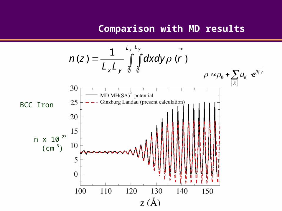
n x 10-23 (cm-3)

0 0

1( ) ( )

yxLL

x y

n z dxdy rL L

0

iK rK

K

u e

Comparison with MD results

BCC Iron

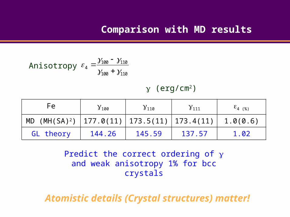
100 1104

100 110

Fe 100 110 111 4 (%)

MD (MH(SA)2) 177.0(11) 173.5(11) 173.4(11) 1.0(0.6)

GL theory 144.26 145.59 137.57 1.02

Predict the correct ordering of and weak anisotropy 1% for bcc crystals

Anisotropy

(erg/cm2)

Comparison with MD results

Atomistic details (Crystal structures) matter!

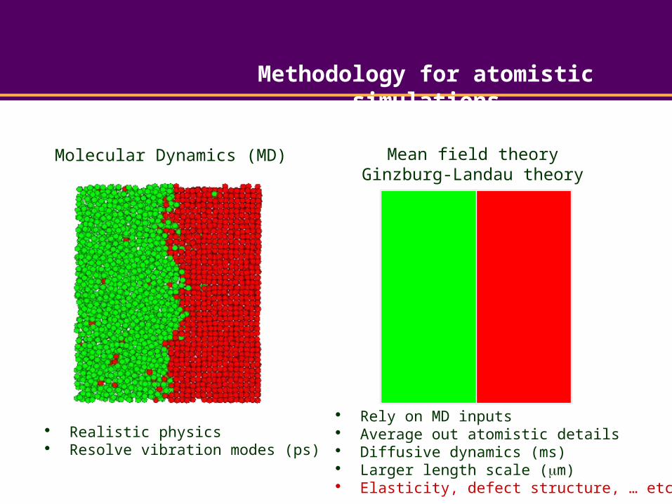
Methodology for atomistic simulations

Molecular Dynamics (MD) Mean field theoryGinzburg-Landau theory

Realistic physics Resolve vibration modes (ps)

0

1

Rely on MD inputs Average out atomistic details Diffusive dynamics (ms) Larger length scale (m) Elasticity, defect structure, … etc?

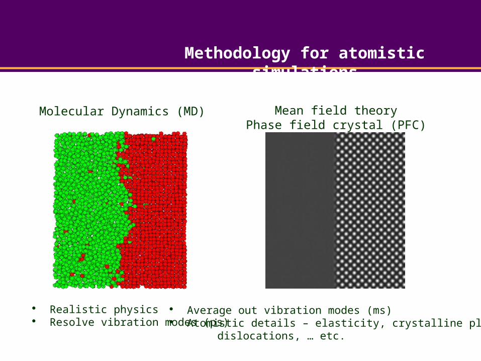
Methodology for atomistic simulations

Molecular Dynamics (MD) Mean field theoryPhase field crystal (PFC)

Average out vibration modes (ms) Atomistic details – elasticity, crystalline planes,

dislocations, … etc.

Realistic physics Resolve vibration modes (ps)

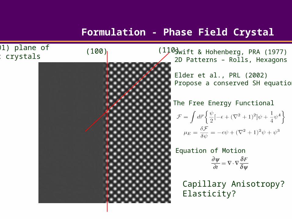
(001) plane of bcc crystals

(100) (110)

Formulation - Phase Field Crystal

Capillary Anisotropy?Elasticity?

Swift & Hohenberg, PRA (1977)2D Patterns – Rolls, Hexagons

Elder et al., PRL (2002)Propose a conserved SH equation

The Free Energy Functional

Equation of Motion

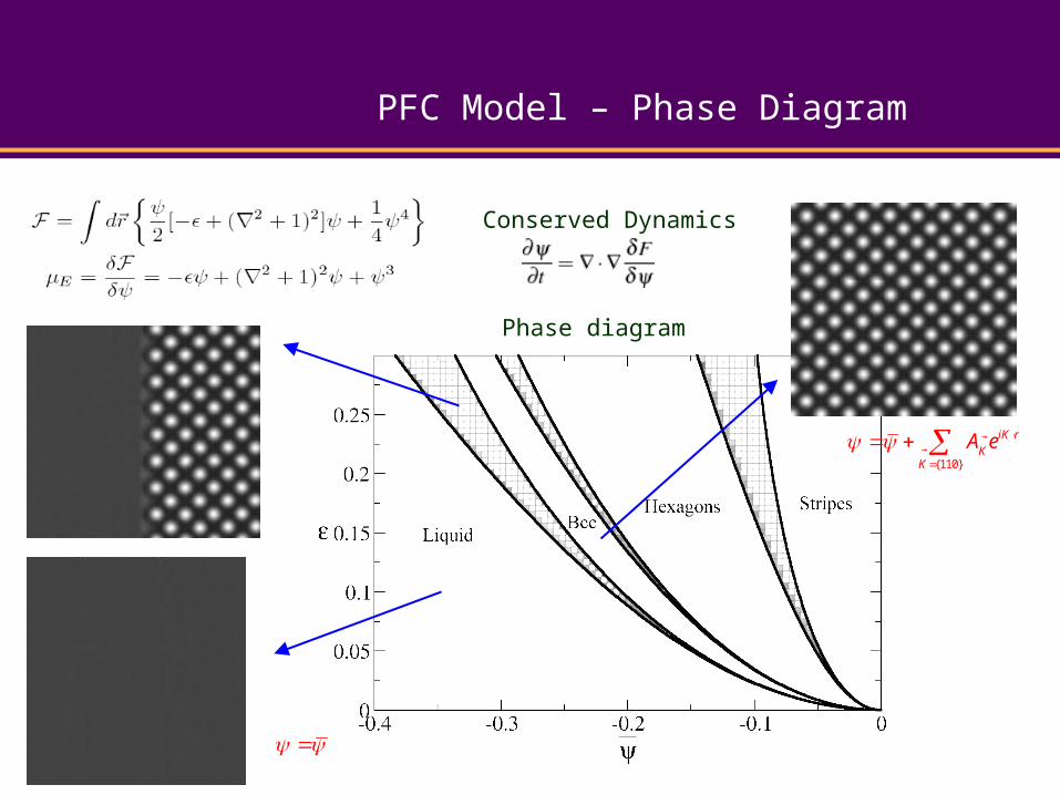
PFC Model – Phase Diagram

{110}

iK rK

K

A e

Phase diagram

Conserved Dynamics

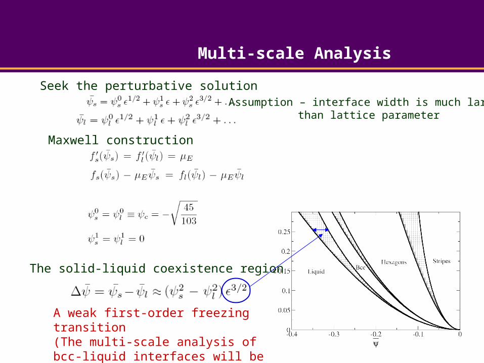
Maxwell construction

Seek the perturbative solution

The solid-liquid coexistence region

A weak first-order freezing transition(The multi-scale analysis of bcc-liquid interfaces will be carried out around c)

Multi-scale Analysis

Assumption – interface width is much larger than lattice parameter

0iA Z

iiK re

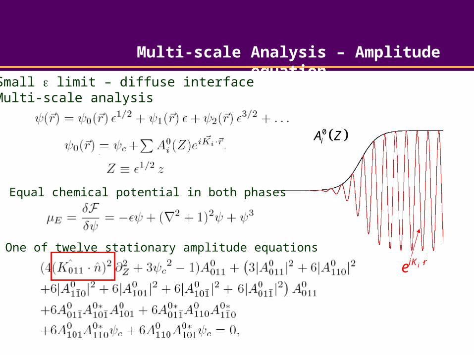
Small limit – diffuse interfaceMulti-scale analysis

Equal chemical potential in both phases

One of twelve stationary amplitude equations

Multi-scale Analysis – Amplitude equation

u110

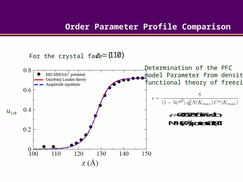
Order Parameter Profile Comparison

(110)z For the crystal face

2

0.0923 for Fe with

MH(SA) potential (MD)

Determination of the PFC model Parameter from densityfunctional theory of freezing

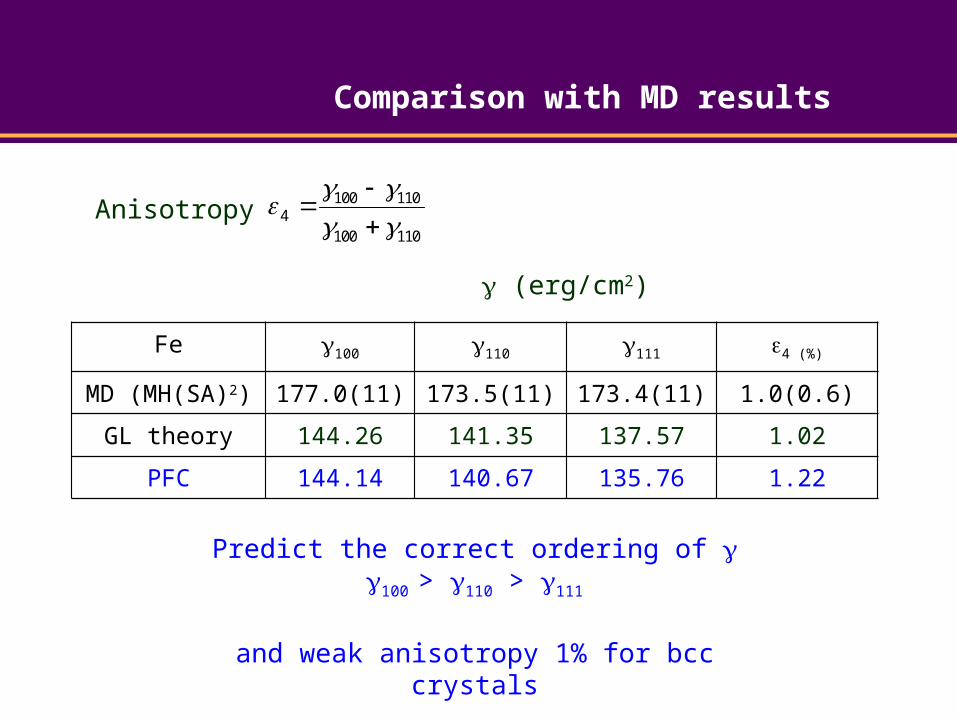
100 1104

100 110

Fe 100 110 111 4 (%)

MD (MH(SA)2) 177.0(11) 173.5(11) 173.4(11) 1.0(0.6)

GL theory 144.26 141.35 137.57 1.02

PFC 144.14 140.67 135.76 1.22

Predict the correct ordering of 100 > 110 > 111

and weak anisotropy 1% for bcc crystals

Anisotropy

(erg/cm2)

Comparison with MD results

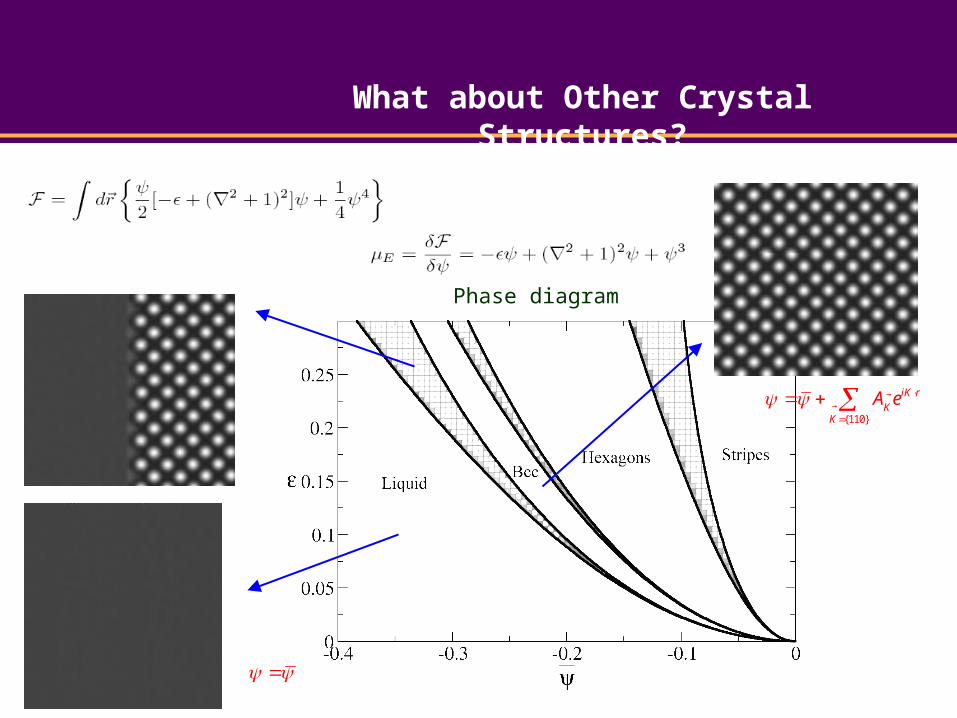
What about Other Crystal Structures?

{110}

iK rK

K

A e

Phase diagram

2 3 42 110 3 110 4 110F a u a u a u

(110)

(011)

(10 1)

F

u110

x

y

z

BCC-Liquid

2 42 200

23 111 200

2 42 111 4 1 01 201 4

b u u

a u bF b u ua u

111 111

200

F

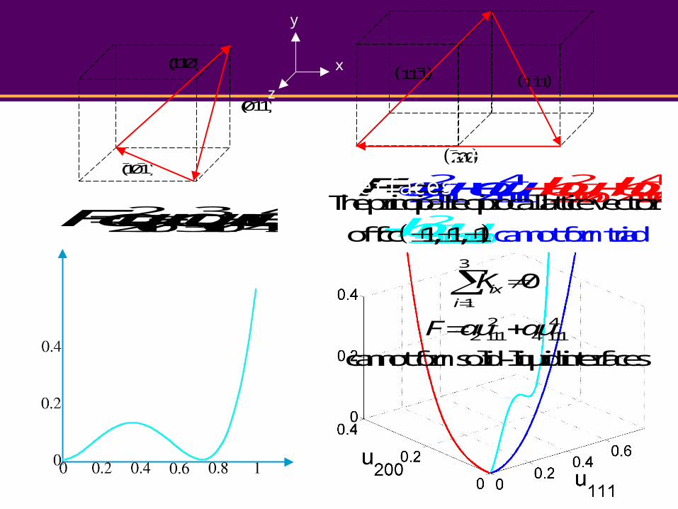
FCC-Liquid

3

1

2 42 111 4 111

1, 1, 1

ixi

K

F a u a u

cannot form

The principal reciprocal lattice vectror

of fcc

0

cannot form solid - liquid interf

triad

aces

GL theory of fcc-liquid interfaces

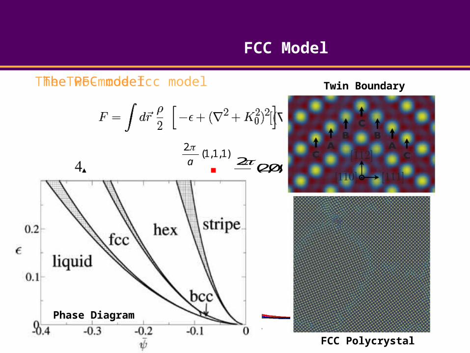
The Two-mode fcc model

2(2,0,0)

a

K

)(KS

2(1,1,1)

a

The PFC model

2

20

2

21

11,1,1 1

3

1 42,0,0

33

K

K

FCC Model

Phase Diagram

Twin Boundary

FCC Polycrystal

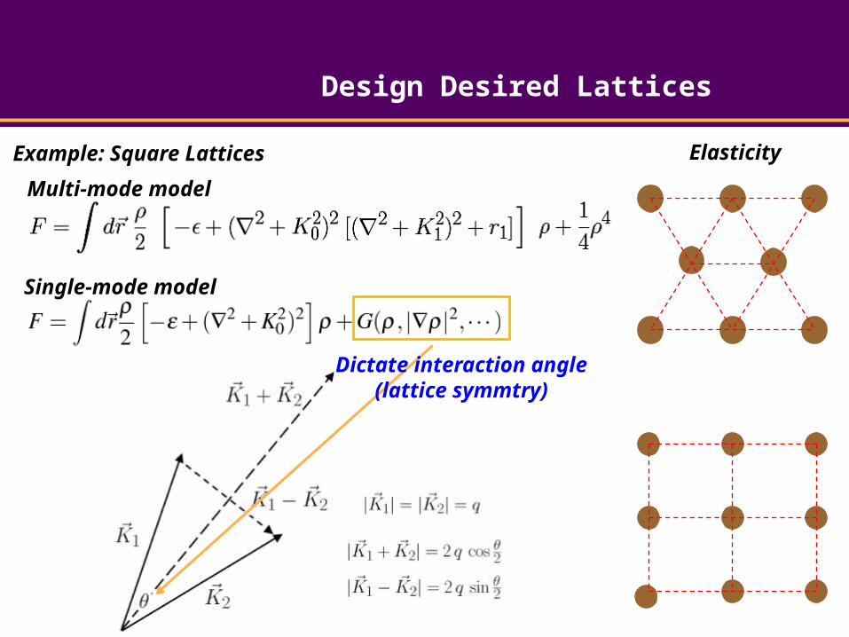
Design Desired Lattices

Example: Square Lattices

Single-mode model

Multi-mode model

Dictate interaction angle(lattice symmtry)

Elasticity

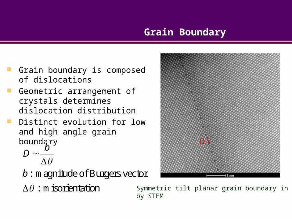
Grain Boundary

Grain boundary is composed of dislocations

Geometric arrangement of crystals determines dislocation distribution

Distinct evolution for low and high angle grain boundary

Symmetric tilt planar grain boundary in goldby STEM

: magnitude of Burgers vector

: misorientation

bD

b

D

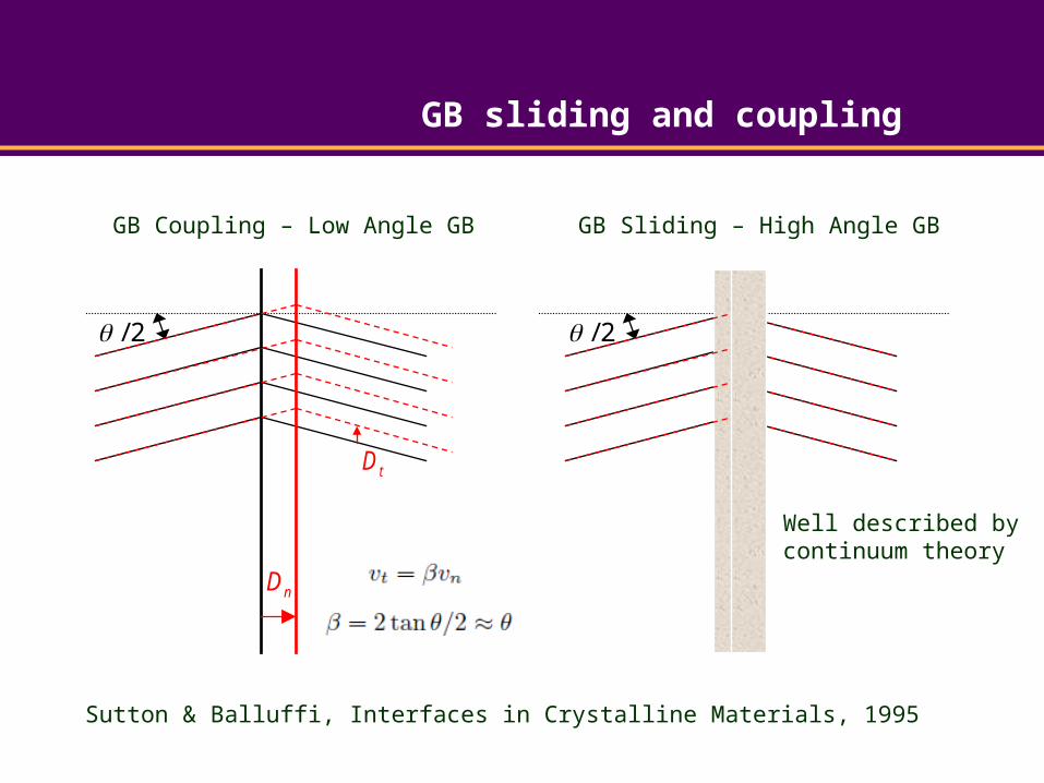
GB sliding and coupling

/ 2

GB Coupling – Low Angle GB GB Sliding – High Angle GB

tD

nD

/ 2

Sutton & Balluffi, Interfaces in Crystalline Materials, 1995

Well described bycontinuum theory

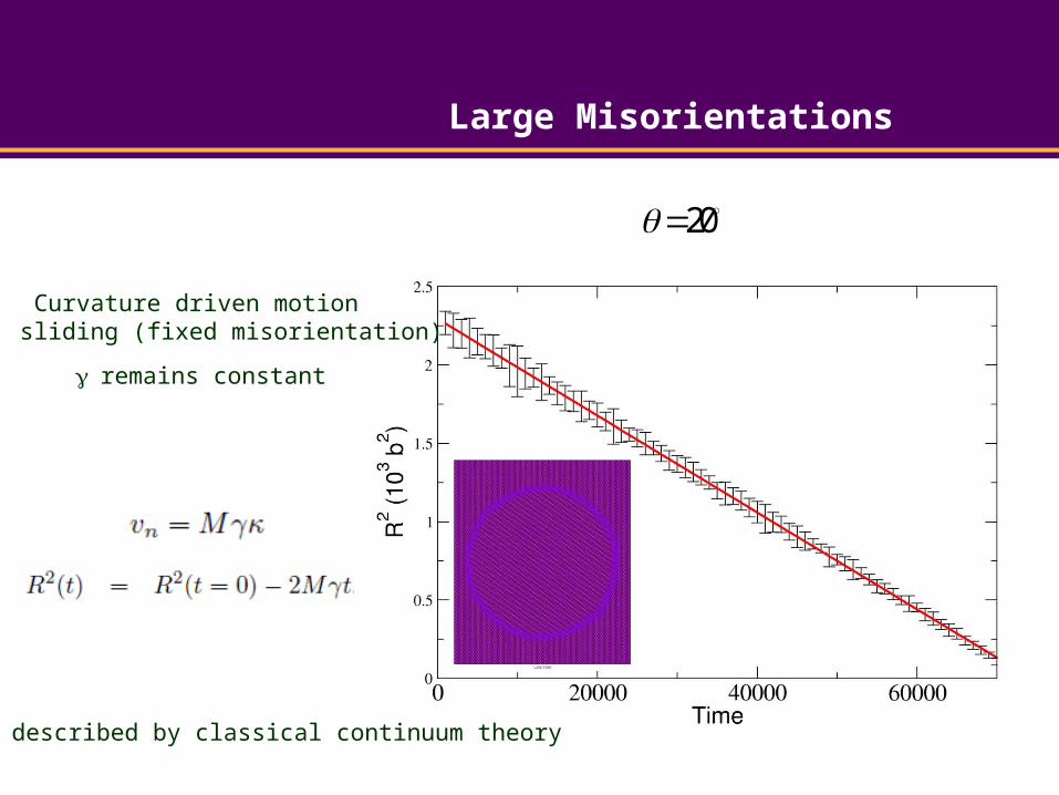
Large Misorientations

Curvature driven motionG.B. sliding (fixed misorientation)

g remains constant

20

Well described by classical continuum theory

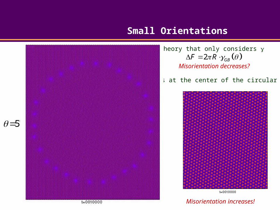
Small Orientations

5

Atoms at the center of the circular grain

2 GBF R Theory that only considers g

Misorientation decreases?

Misorientation increases!

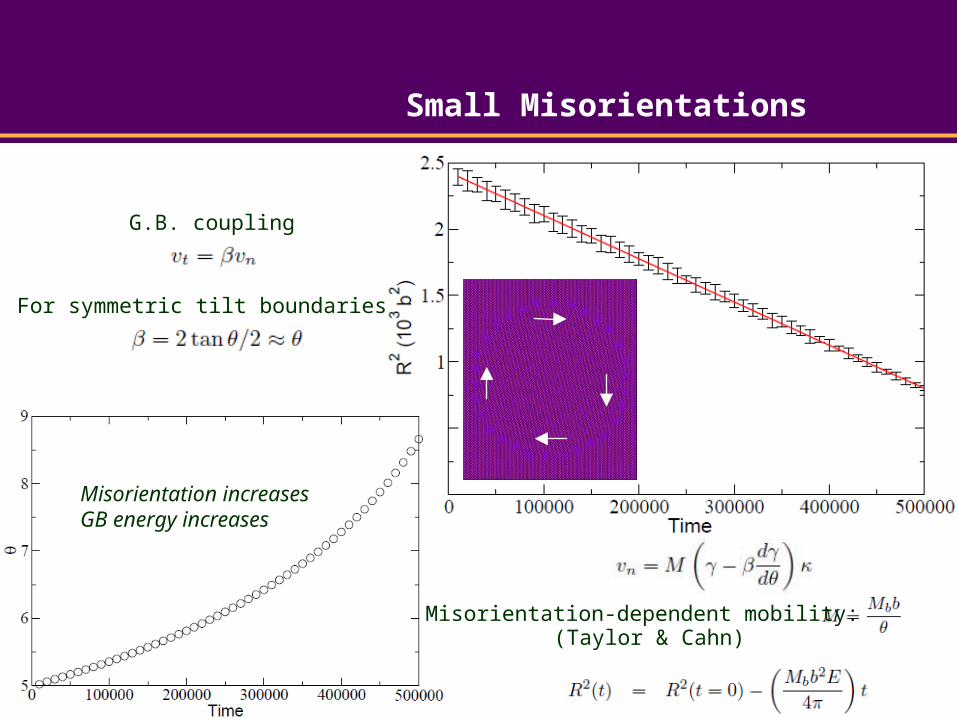
Small Misorientations

G.B. coupling

Misorientation-dependent mobility:

For symmetric tilt boundaries

(Taylor & Cahn)

Misorientation increasesGB energy increases

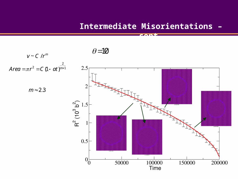
22 1

~ /

(1 )

m

m

v C r

Area r C at

Intermediate Misorientations – cont.

2.3m

10

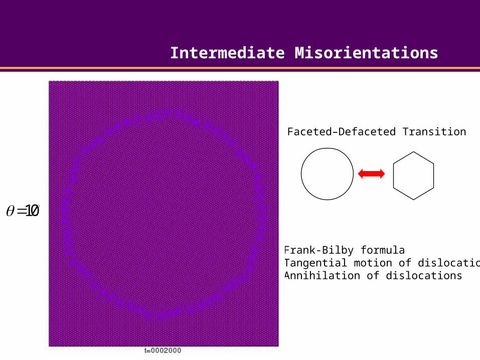
Intermediate Misorientations

10

Faceted–Defaceted Transition

Frank-Bilby formula Tangential motion of dislocations Annihilation of dislocations

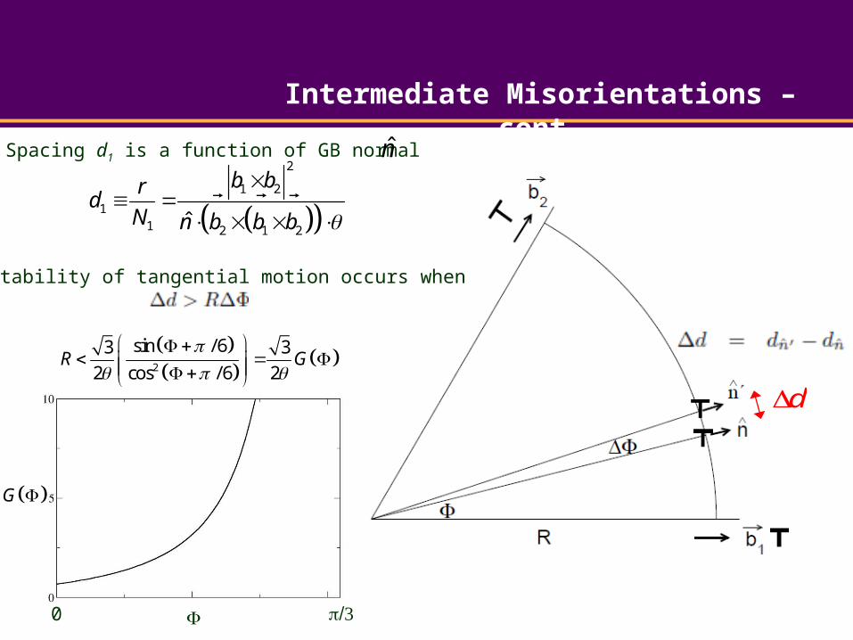
Intermediate Misorientations – cont.

d

Instability of tangential motion occurs when

2

1 2

11 2 1 2ˆ

b brd

N n b b b

0 /3pF

2

sin / 63 3

2 cos / 6 2R G

G

Spacing d1 is a function of GB normal n

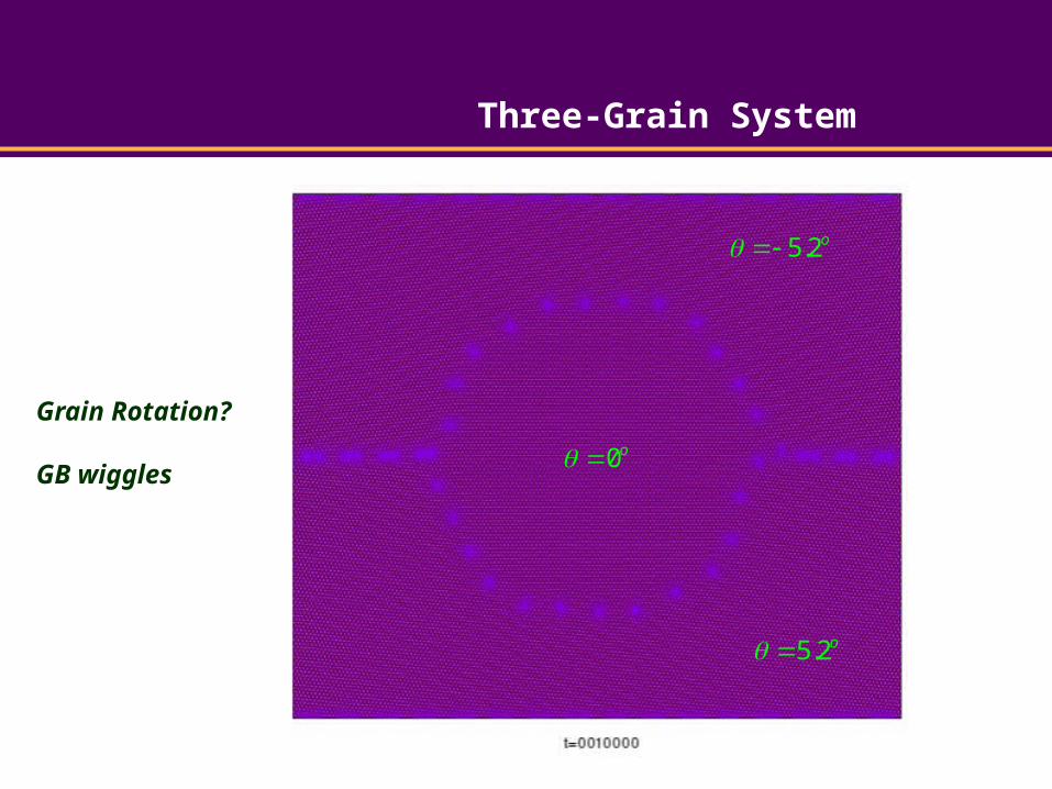
Three-Grain System

5.2o

5.2o

0o

Grain Rotation?

GB wiggles

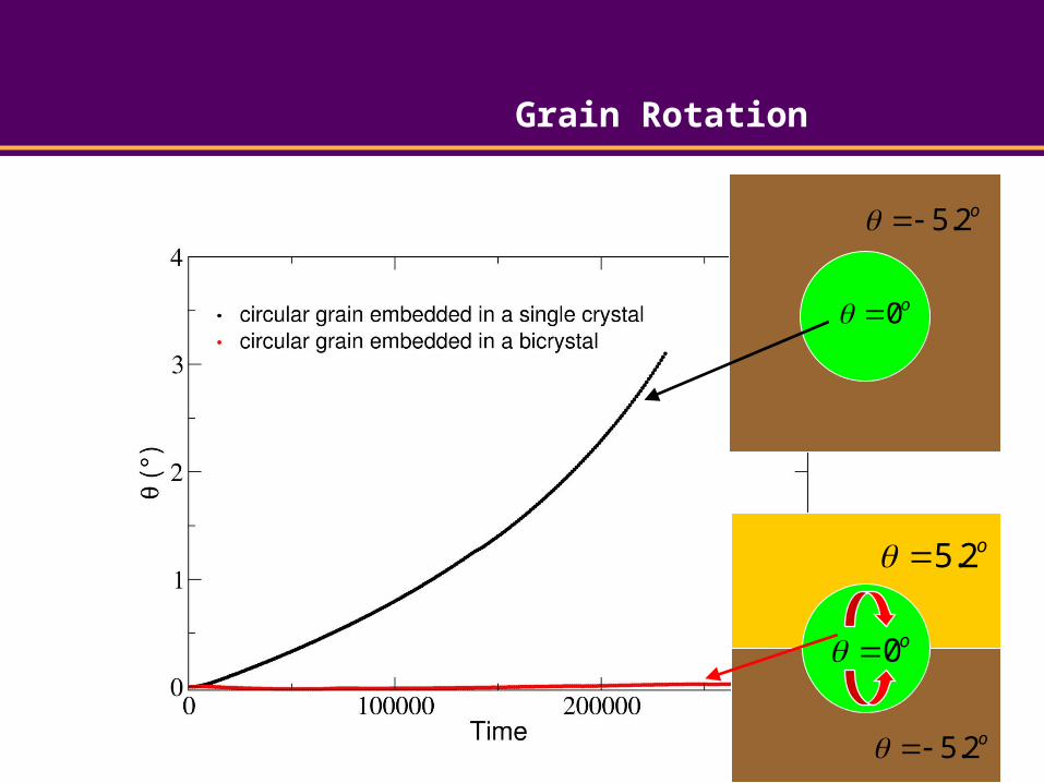
Grain Rotation

5.2o

0o

5.2o

0o

5.2o

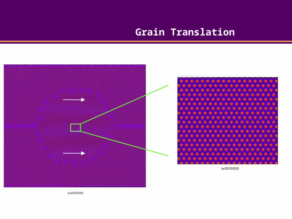
Grain Translation

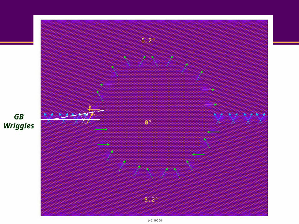
5.2º

-5.2º

0ºGB

Wriggles

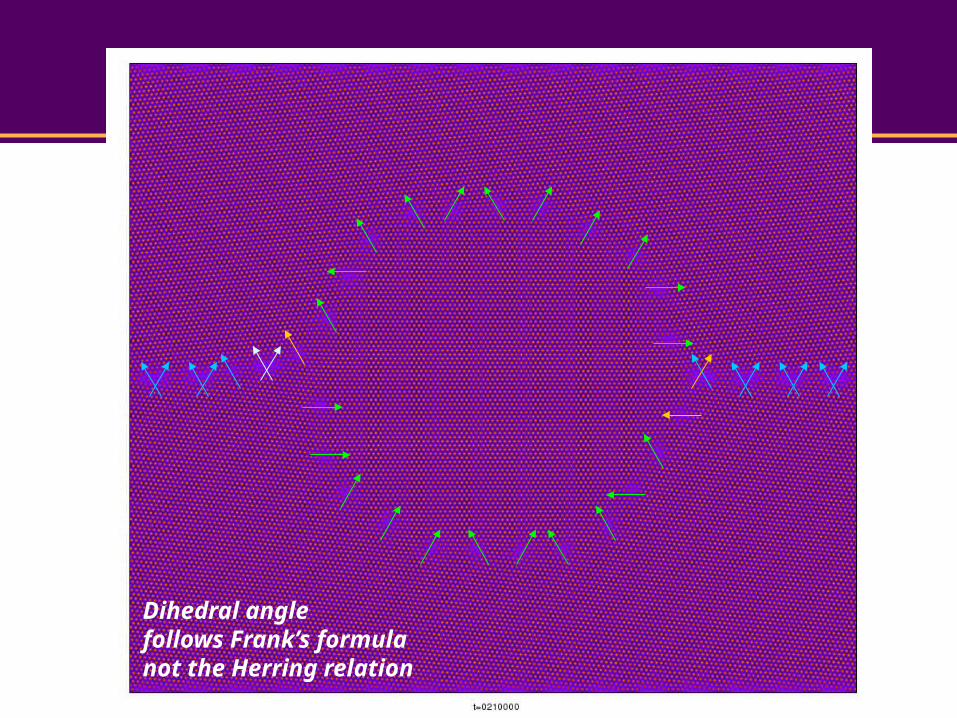
Dihedral anglefollows Frank’s formulanot the Herring relation

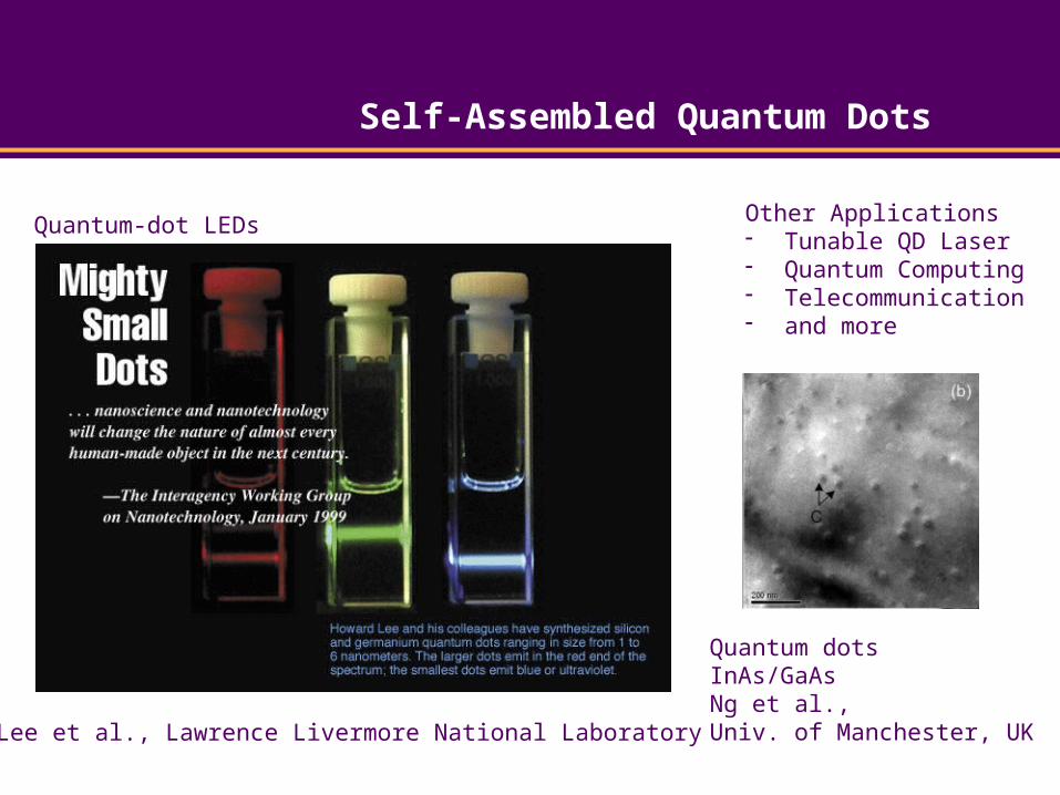
Self-Assembled Quantum Dots

Lee et al., Lawrence Livermore National Laboratory

Quantum-dot LEDs Other Applications- Tunable QD Laser- Quantum Computing- Telecommunication- and more

Quantum dots InAs/GaAsNg et al., Univ. of Manchester, UK

ˆ exp x yh ik x ik y

2 2 2ˆ , ,

22 10 100 nmc

c

Uh k E E k

A

k E

Linear perturbationcalculation

k

UA

ck

Film

Substrate

h

z

x

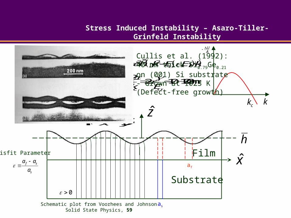
Stress Induced Instability – Asaro-Tiller-Grinfeld Instability

f s

s

a a

a

0

Schematic plot from Voorhees and JohnsonSolid State Physics, 59

Cullis et al. (1992): 40 nm thick Si0.79Ge0.21 on (001) Si substrate - Grown at 1023 K (Defect-free growth)

Misfit Parameter

as

af

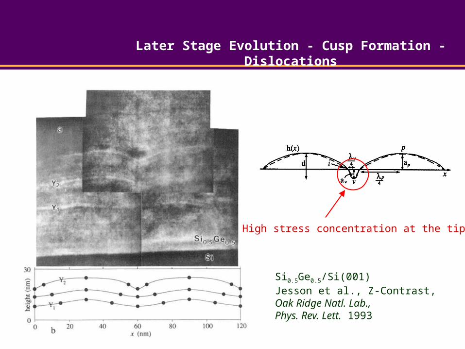
Later Stage Evolution - Cusp Formation - Dislocations

Si0.5Ge0.5/Si(001)Jesson et al., Z-Contrast, Oak Ridge Natl. Lab., Phys. Rev. Lett. 1993

High stress concentration at the tip

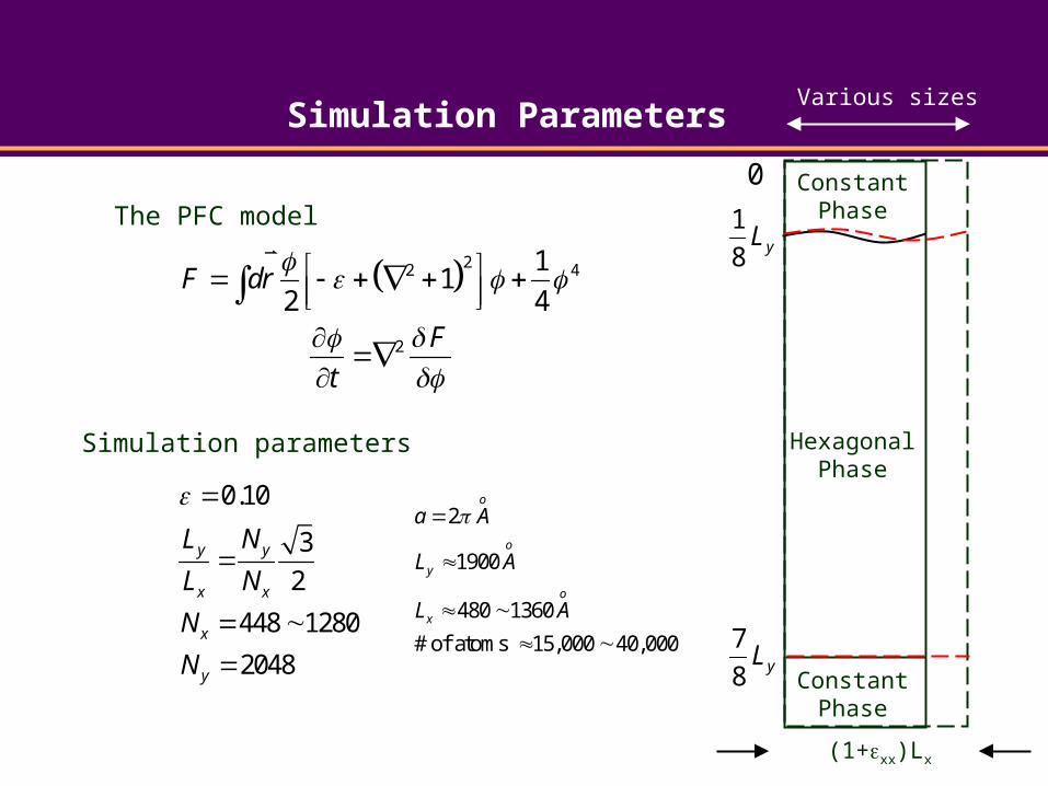
Simulation Parameters

0.10

3

2

448 1280

2048

y y

x x

x

y

L N

L N

N

N

yL8

1

yL8

7

0

22 4

2

11

2 4F dr

F

t

The PFC model

Simulation parameters

Various sizes

HexagonalPhase

ConstantPhase

ConstantPhase

(1+xx)Lx

2

1900

480 1360

# of atoms 15,000 40,000

o

o

y

o

x

a A

L A

L A

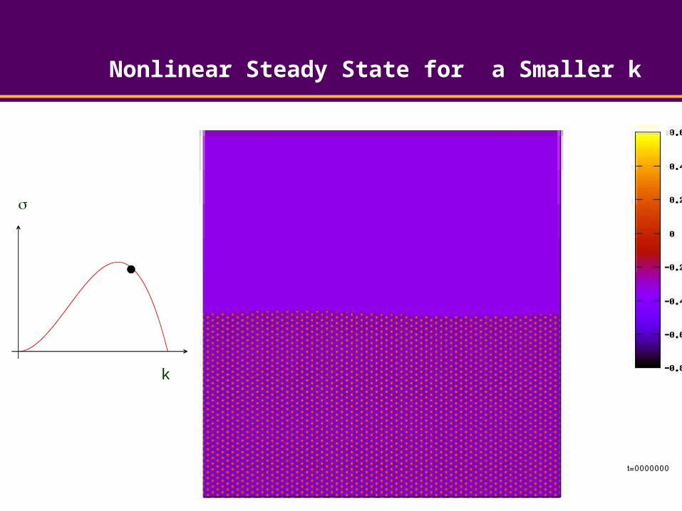
Nonlinear Steady State for a Smaller k

k

ˆxxˆyy

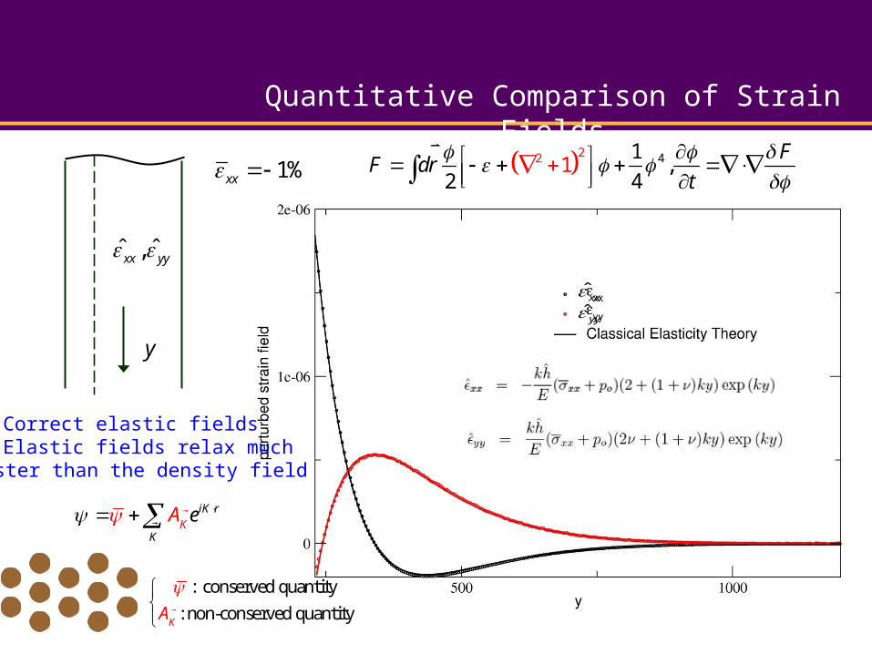
Quantitative Comparison of Strain Fields

1%xx 422 1,

2 41

FF dr

t

ˆ ˆ,xx yy

y

Correct elastic fields Elastic fields relax much faster than the density field

iK

K r

K

eA

: conserved quantity

: non-conserved quantityKA

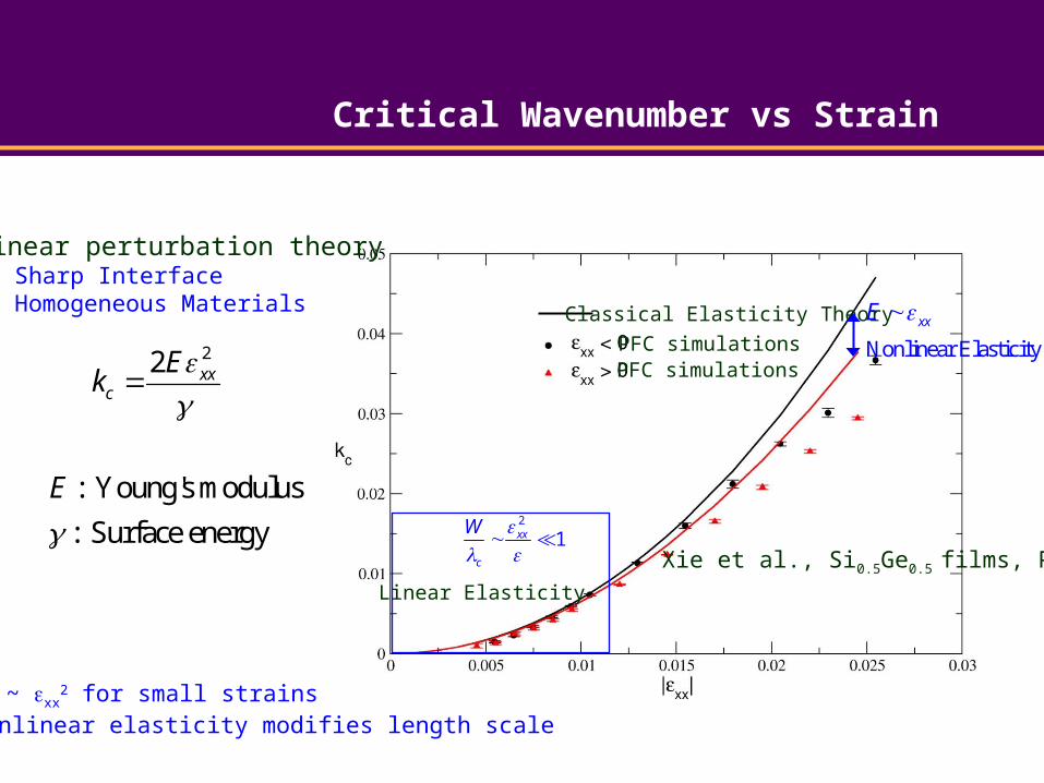
Critical Wavenumber vs Strain

Linear perturbation theory- Sharp Interface- Homogeneous Materials

22 xxc

Ek

: Young's modulus

: Surface energy

E

PFC simulationsPFC simulations

Classical Elasticity Theory

Nonlinear Elasticity

xxE

Xie et al., Si0.5Ge0.5 films, PRL

2

1xx

c

W

Linear Elasticity

kc ~ xx2 for small strains

Nonlinear elasticity modifies length scale

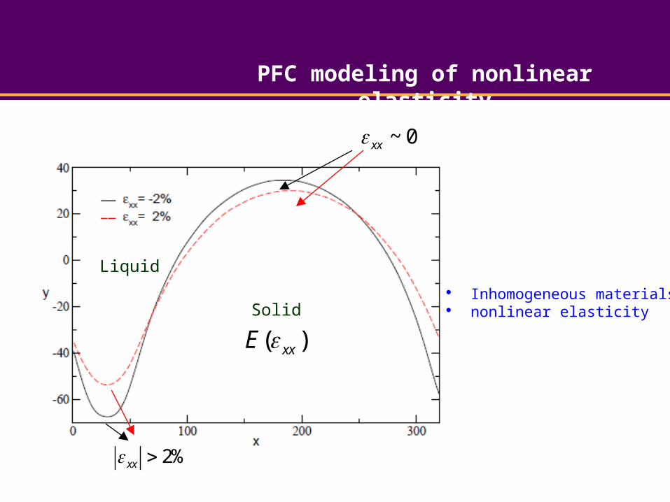
PFC modeling of nonlinear elasticity

Solid

Liquid

( )xxE

~ 0xx

2%xx

Inhomogeneous materials nonlinear elasticity

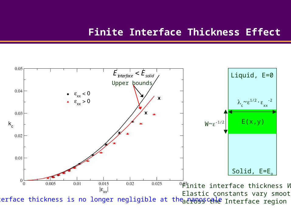
Finite Interface Thickness Effect

Solid, E=Eo

Liquid, E=0

E(x,y)

c~1/2·

xx-2

W~-1/2

Finite interface thickness WElastic constants vary smoothlyacross the Interface region

Upper boundsint erface solidE E

Interface thickness is no longer negligible at the nanoscale

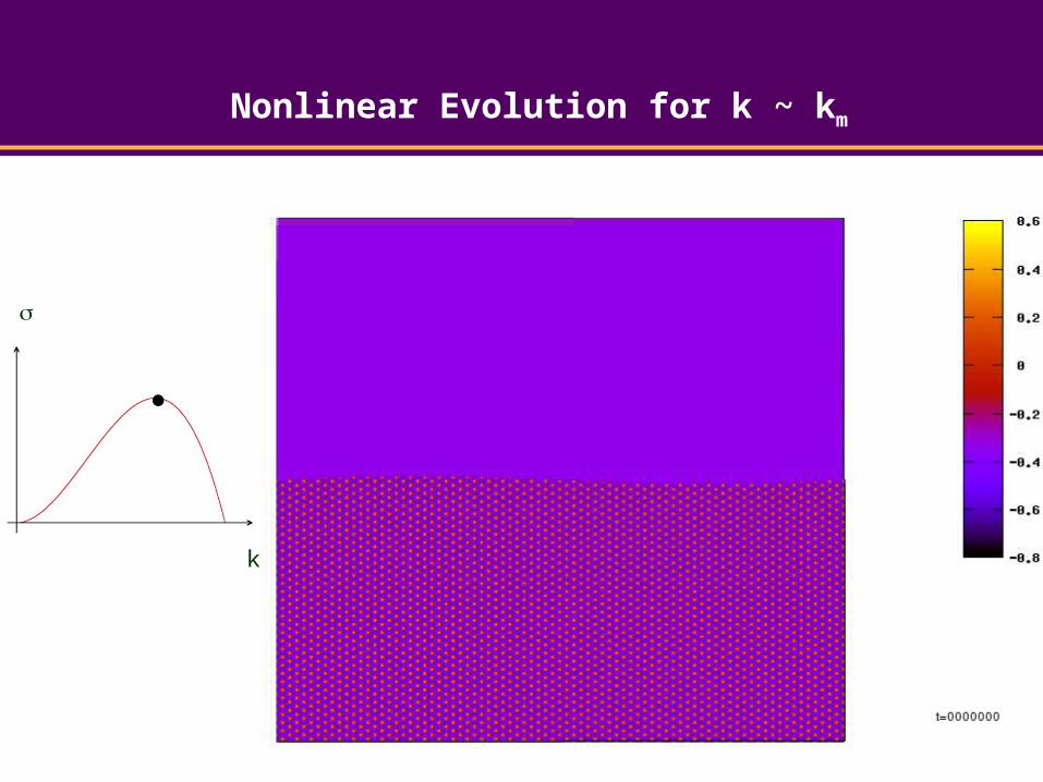
Nonlinear Evolution for k ~ km

k

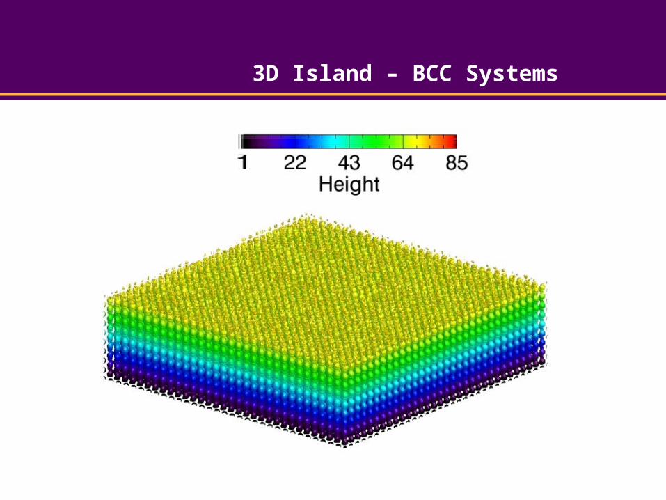
3D Island – BCC Systems

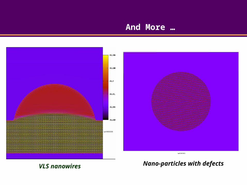
And More …

VLS nanowires Nano-particles with defects

And More …

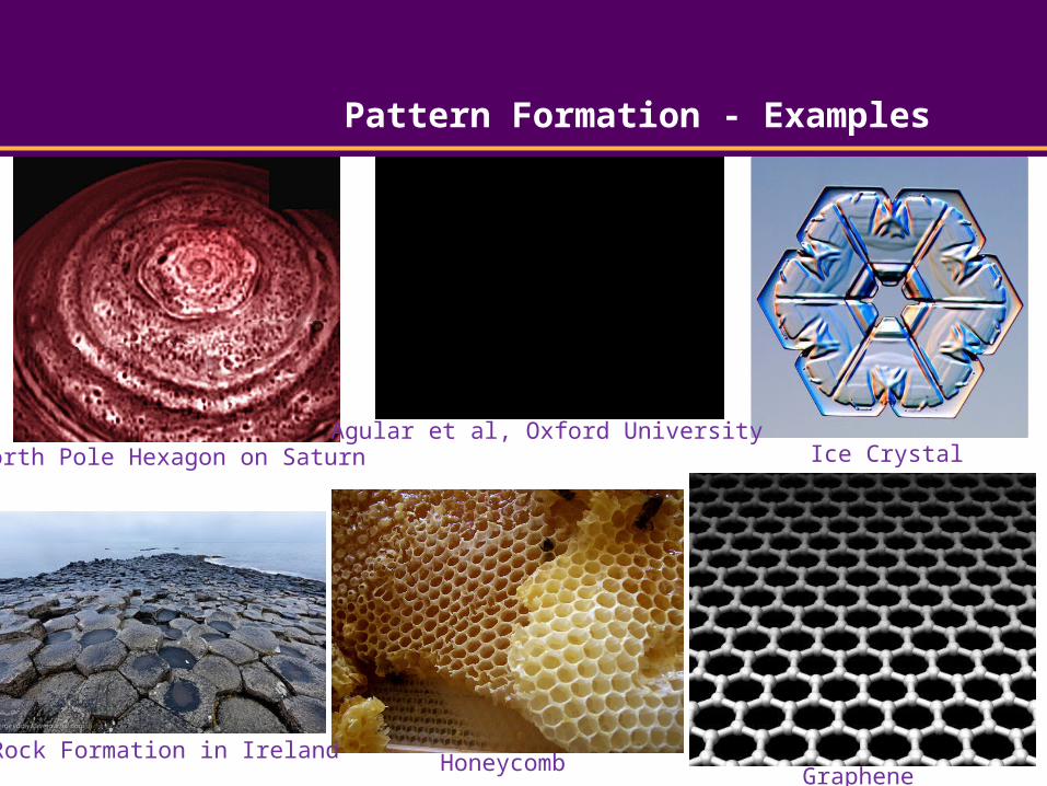
Pattern Formation - Examples

Graphene

North Pole Hexagon on Saturn Ice CrystalAgular et al, Oxford University

HoneycombRock Formation in Ireland

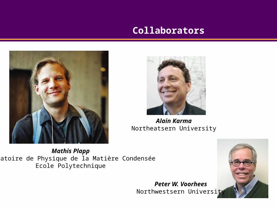
Collaborators

Mathis PlappLaboratoire de Physique de la Matière Condensée 

Ecole Polytechnique

Alain KarmaNortheatsern University

Peter W. VoorheesNorthwestsern University