Embed Size (px)
Citation preview
micromachines
Article
Full-Azimuth Beam Steering MIMO AntennaArranged in a Daisy Chain Array Structure
Kazuhiro Honda 1,*, Taiki Fukushima 2 and Koichi Ogawa 1
1 Graduate School of Engineering, Toyama University, 3190 Gofuku, Toyama 930-8555, Japan;[email protected]
2 Panasonic System Networks R&D Lab. Co., Ltd., Technology Center, 2-5 Akedori, Izumi-ku, Sendai,Miyagi 981-3206, Japan; [email protected]
* Correspondence: [email protected]; Tel.: +81-76-445-6759
Received: 28 August 2020; Accepted: 18 September 2020; Published: 19 September 2020�����������������
Abstract: This paper presents a multiple-input, multiple-output (MIMO) antenna system with theability to perform full-azimuth beam steering, and with the aim of realizing greater than 20 Gbpsvehicular communications. The MIMO antenna described in this paper comprises 64 elementsarranged in a daisy chain array structure, where 32 subarrays are formed by pairing elements ineach subarray; the antenna yields 32 independent subchannels for MIMO transmission, and coversall communication targets regardless of their position relative to the array. Analytical results revealthat the proposed antenna system can provide a channel capacity of more than 200 bits/s/Hz at asignal-to-noise power ratio (SNR) of 30 dB over the whole azimuth, which is equivalent to 20 Gbpsfor a bandwidth of 100 MHz. This remarkably high channel capacity is shown to be due to twosignificant factors; the improved directivity created by the optimum in-phase excitation and thelow correlation between the subarrays due to the orthogonal alignment of the array with respectto the incident waves. Over-the-air (OTA) experiments confirm the increase in channel capacity;the proposed antenna can maintain a constant transmission rate over all azimuth angles.
Keywords: daisy chain multiple-input multiple-output (MIMO) antenna; beam steering array;large-scale MIMO; over-the-air (OTA) testing; Monte Carlo simulation; connected car
1. Introduction
One of the most straightforward approaches for improving the capacity of multiple-inputmultiple-output (MIMO) systems is to use a large number of antenna elements. The concept oflarge-scale MIMO or massive MIMO systems with more than 100 antenna elements has been proposedfor both fifth and sixth generation (5G and 6G) mobile communications [1,2].
Figure 1 shows a conceptual illustration of a massive MIMO system. In massive MIMO systems,investigations are mostly based on the development of a large-scale antenna at a base station, in whicha planar array antenna with a number of patch antennas arranged in a two-dimensional manner ona column-row alignment basis is commonly developed [3–6], as depicted in Figure 1. The primaryobjective of these antennas is, using a beam forming technique, to illuminate respective mobilestations distributed in a specific confined region of the service area in a cell, known as a hot-spot.Thus, a large-scale MIMO antenna used for massive MIMO systems is capable of communicating withmobile stations in the hemispherical spatial region perpendicular to the surface of the patch array.With regard to a mobile station antenna, on the other hand, one of the most important performance goalsin MIMO systems is the ability to communicate with the target over the full azimuth, i.e., full-azimuthbeam steering, as illustrated in Figure 1.
Micromachines 2020, 11, 871; doi:10.3390/mi11090871 www.mdpi.com/journal/micromachines

Micromachines 2020, 11, 871 2 of 25Micromachines 2020, 11, x 2 of 25
Figure 1. Conceptual illustration of a massive MIMO system.
One of the possible solutions to fulfilling this requirement is the use of a circular array in which
a number of patch antennas are arranged in a cylindrical manner [7,8]. However, there is a certain
drawback to this configuration in that each patch antenna radiates in a direction normal to the surface
of the patch, resulting in a situation in which not all of the radiation beams contribute to MIMO
spatial multiplexing when an incident wave comes from a particular azimuthal direction.
Consequently, we cannot obtain full-rank channel matrices corresponding to the number of patches
due to the limited availability of the received signals, which leads to a reduction in channel capacity.
There has been a great deal of interest in the development of connected car systems with greater
than a gigabit transmission rates [9]. It is anticipated that the MIMO antennas implemented in
automobiles will be used in systems with a relatively small cell radius involving a street microcell
[10]. In such an environment, the various objects in the surrounding area—such as trees, signboards,
buildings, and numerous vehicles—result in complex radio propagation phenomena. In a street
microcell environment, it is known that the spatial angular power spectrum (APS) is small compared
with that in the conventional macrocell counterpart [11]. This is because the incident waves from
these scatterers are not uniformly distributed, but occur in clusters, with strong contributions from a
few directions. In addition, the radiation pattern of a vehicular antenna changes greatly due to the
mutual electromagnetic coupling between the antenna and the dynamic motion of the car, especially
when it turns right or left at an intersection. This indicates that the mutual influence of the incident
waves and the car’s antennas could result in a complicated MIMO channel response.
Based on the above-mentioned phenomena, the characteristics of a vehicular MIMO antenna are
summarized as follows:
(1) Anticipated changes in received power when the position of the car changes relative to the
incident waves.
(2) Increase in spatial fading correlation between the array branches due to the narrow APS.
(3) Changes in both the received power and correlation, which may be encountered at the same
time, as the car moves in different directions relative to the incident waves.
(4) A possible increase or decrease in the MIMO channel capacity caused by (1), (2), or (3).
These phenomena may occur simultaneously in an actual connected car system. Hence, all the
solutions with regard to the above issues must be integrated into one unit in the developed MIMO
antenna. Considering this technical background, we have developed new technologies in an ongoing
project with the following objectives:
(A) Development of higher order MIMO arrays, such as 8 × 8 [12], 16 × 16 [13], and 32 × 32 [14,15]
MIMO antenna systems, suitable for implementation in an automobile.
Mobile station
Large-scale MIMO antenna
Patch array
Base station
Full-azimuth beam steering
MIMO transmission
Figure 1. Conceptual illustration of a massive MIMO system.
One of the possible solutions to fulfilling this requirement is the use of a circular array in whicha number of patch antennas are arranged in a cylindrical manner [7,8]. However, there is a certaindrawback to this configuration in that each patch antenna radiates in a direction normal to the surfaceof the patch, resulting in a situation in which not all of the radiation beams contribute to MIMO spatialmultiplexing when an incident wave comes from a particular azimuthal direction. Consequently,we cannot obtain full-rank channel matrices corresponding to the number of patches due to the limitedavailability of the received signals, which leads to a reduction in channel capacity.
There has been a great deal of interest in the development of connected car systems with greaterthan a gigabit transmission rates [9]. It is anticipated that the MIMO antennas implemented inautomobiles will be used in systems with a relatively small cell radius involving a street microcell [10].In such an environment, the various objects in the surrounding area—such as trees, signboards,buildings, and numerous vehicles—result in complex radio propagation phenomena. In a streetmicrocell environment, it is known that the spatial angular power spectrum (APS) is small comparedwith that in the conventional macrocell counterpart [11]. This is because the incident waves from thesescatterers are not uniformly distributed, but occur in clusters, with strong contributions from a fewdirections. In addition, the radiation pattern of a vehicular antenna changes greatly due to the mutualelectromagnetic coupling between the antenna and the dynamic motion of the car, especially when itturns right or left at an intersection. This indicates that the mutual influence of the incident waves andthe car’s antennas could result in a complicated MIMO channel response.
Based on the above-mentioned phenomena, the characteristics of a vehicular MIMO antenna aresummarized as follows:
(1) Anticipated changes in received power when the position of the car changes relative to theincident waves.
(2) Increase in spatial fading correlation between the array branches due to the narrow APS.(3) Changes in both the received power and correlation, which may be encountered at the same time,
as the car moves in different directions relative to the incident waves.(4) A possible increase or decrease in the MIMO channel capacity caused by (1), (2), or (3).
These phenomena may occur simultaneously in an actual connected car system. Hence, all thesolutions with regard to the above issues must be integrated into one unit in the developed MIMOantenna. Considering this technical background, we have developed new technologies in an ongoingproject with the following objectives:
Micromachines 2020, 11, 871 3 of 25
(A) Development of higher order MIMO arrays, such as 8 × 8 [12], 16 × 16 [13], and 32 × 32 [14,15]MIMO antenna systems, suitable for implementation in an automobile.
(B) Development of radiation pattern steering capability to achieve a large signal-to-noise powerratio (SNR) that can direct the peak radiation toward the communication target.
(C) Realization of low correlation between the MIMO channels established by the orthogonalrelationship between the array alignment and the incident waves over the full azimuth.
(D) Development of an angle of arrival (AOA) estimation antenna that obtains bearing informationfrom radio waves incident on the MIMO antenna, using an RF-based interferometric monopulsetechnique with reduced hardware complexity.
To realize these objectives simultaneously, we are currently developing a 32 × 32 MIMO antennasystem that utilizes circular array beam steering technology. Great emphasis is placed on a way ofachieving a large-scale vehicle borne MIMO antenna that provides full-azimuth coverage. The new arrayconfiguration proposed in this paper yields the full availability of the received signals, which resultsin a channel capacity of several tens of gigabits owing to the effective operation of the MIMOmultiplexing transmission.
This paper, which is part of the extensive R&D activities we have performed so far in this field,is devoted to a comprehensive description of the development work undertaken for a 32 × 32 MIMOantenna system, including Monte Carlo simulations and over-the-air (OTA) testing to investigate howthe developed 32 × 32 MIMO array performs in a propagation environment where it is anticipated theforthcoming 5G and 6G connected car systems will be used.
In order to tackle the four challenges—(A), (B), (C), and (D), listed above—we start by describingthe methodology and the basic characteristics of MIMO antennas. We first present a brief explanationof the configuration of the whole antenna system. Studies on the AOA antenna are presented inseparate papers [16,17].
2. New Concept of a Large-Scale MIMO Antenna
In Figure 2 an illustrated overview of our ongoing project, conducting research and developmentwork toward a full-azimuth beam steering MIMO array, is shown [18]. We have taken on thebig challenge of achieving a 100 Gbps channel capacity on a moving vehicle for the forthcomingsixth-generation (6G) mobile communications. To this end, we have devised effective means ofconstructing a large-scale MIMO array antenna, with distinct features that cannot be achievedusing previous technologies commonly aimed at enhancing the channel capacity at a base station;the objective of our project is accomplished by the emergence of a new technology named “Daisy ChainMIMO Antenna”.
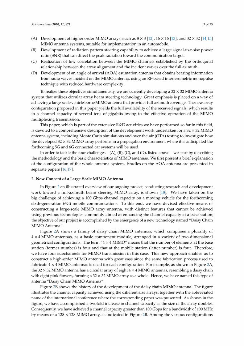
Figure 2A shows a family of daisy chain MIMO antennas, which comprises a plurality of4 × 4 MIMO antennas, as a basic component module, arranged in a variety of two-dimensionalgeometrical configurations. The term “4 × 4 MIMO” means that the number of elements at the basestation (former number) is four and that at the mobile station (latter number) is four. Therefore,we have four subchannels for MIMO transmission in this case. This new approach enables us toconstruct a high-order MIMO antenna with great ease since the same fabrication process used tofabricate 4 × 4 MIMO antennas is used for each configuration. For example, as shown in Figure 2A,the 32 × 32 MIMO antenna has a circular array of eight 4 × 4 MIMO antennas, resembling a daisy chainwith eight pink flowers, forming a 32 × 32 MIMO array as a whole. Hence, we have named this type ofantenna “Daisy Chain MIMO Antenna”.
Figure 2B shows the history of the development of the daisy chain MIMO antenna. The figureillustrates the channel capacity achieved using the different size arrays, together with the abbreviatedname of the international conference where the corresponding paper was presented. As shown in thefigure, we have accomplished a twofold increase in channel capacity as the size of the array doubles.Consequently, we have achieved a channel capacity greater than 100 Gbps for a bandwidth of 100 MHzby means of a 128 × 128 MIMO array, as indicated in Figure 2B. Among the various configurations
Micromachines 2020, 11, 871 4 of 25
categorized in the family in Figure 2A, this paper focuses on a detailed description of the design andperformance of a daisy chain 32 × 32 MIMO antenna.
Micromachines 2020, 11, x 3 of 25
(B) Development of radiation pattern steering capability to achieve a large signal-to-noise power ratio (SNR) that can direct the peak radiation toward the communication target.
(C) Realization of low correlation between the MIMO channels established by the orthogonal relationship between the array alignment and the incident waves over the full azimuth.
(D) Development of an angle of arrival (AOA) estimation antenna that obtains bearing information from radio waves incident on the MIMO antenna, using an RF-based interferometric monopulse technique with reduced hardware complexity.
To realize these objectives simultaneously, we are currently developing a 32 × 32 MIMO antenna system that utilizes circular array beam steering technology. Great emphasis is placed on a way of achieving a large-scale vehicle borne MIMO antenna that provides full-azimuth coverage. The new array configuration proposed in this paper yields the full availability of the received signals, which results in a channel capacity of several tens of gigabits owing to the effective operation of the MIMO multiplexing transmission.
This paper, which is part of the extensive R&D activities we have performed so far in this field, is devoted to a comprehensive description of the development work undertaken for a 32 × 32 MIMO antenna system, including Monte Carlo simulations and over-the-air (OTA) testing to investigate how the developed 32 × 32 MIMO array performs in a propagation environment where it is anticipated the forthcoming 5G and 6G connected car systems will be used.
In order to tackle the four challenges—(A), (B), (C), and (D), listed above—we start by describing the methodology and the basic characteristics of MIMO antennas. We first present a brief explanation of the configuration of the whole antenna system. Studies on the AOA antenna are presented in separate papers [16,17].
2. New Concept of a Large-Scale MIMO Antenna
In Figure 2 an illustrated overview of our ongoing project, conducting research and development work toward a full-azimuth beam steering MIMO array, is shown [18]. We have taken on the big challenge of achieving a 100 Gbps channel capacity on a moving vehicle for the forthcoming sixth-generation (6G) mobile communications. To this end, we have devised effective means of constructing a large-scale MIMO array antenna, with distinct features that cannot be achieved using previous technologies commonly aimed at enhancing the channel capacity at a base station; the objective of our project is accomplished by the emergence of a new technology named “Daisy Chain MIMO Antenna”.
(A) (B)
Figure 2. A big challenge toward 100 Gbps channel capacity. (A) A family of daisy chain MIMO antennas. (B) History of the development.
(a) 4 × 4 MIMO (c) 16 × 16 MIMO
(d) 32 × 32 MIMO (e) 64 × 64 MIMO (f) 128 × 128 MIMO
(b) 8 × 8 MIMO
0
200
400
600
800
1000
1200
Chan
nel C
apac
ity [b
its/s
/Hz]
16×16 32×328×84×4 64×64 128×128
SNR=30dBAPMC2017PIERS2018
APMC2018EMTS2019
EMTS2019
100Gbps @100MHz
PIERS2019
This Paper
Figure 2. A big challenge toward 100 Gbps channel capacity. (A) A family of daisy chain MIMOantennas. (B) History of the development.
3. Daisy Chain 32 × 32 Multiple-Input Multiple-Output (MIMO) Antenna
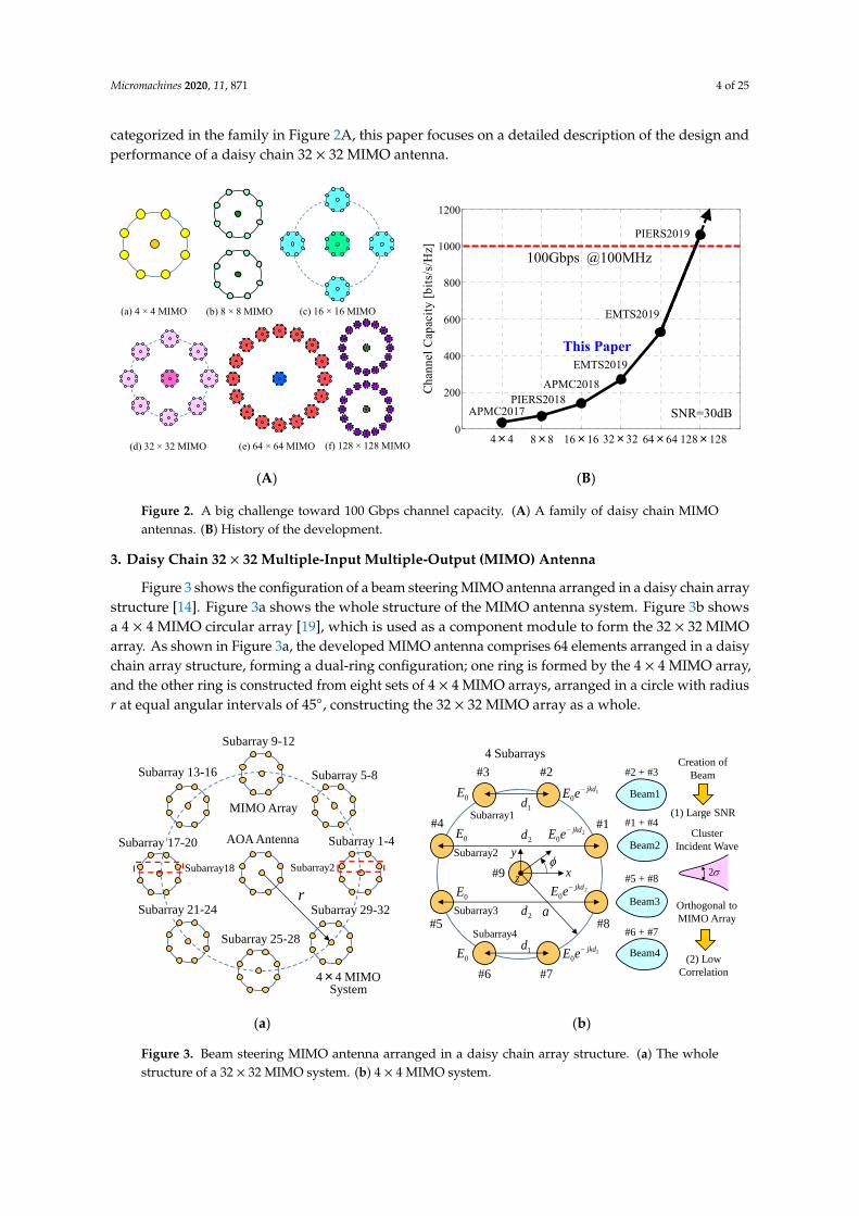
Figure 3 shows the configuration of a beam steering MIMO antenna arranged in a daisy chain arraystructure [14]. Figure 3a shows the whole structure of the MIMO antenna system. Figure 3b showsa 4 × 4 MIMO circular array [19], which is used as a component module to form the 32 × 32 MIMOarray. As shown in Figure 3a, the developed MIMO antenna comprises 64 elements arranged in a daisychain array structure, forming a dual-ring configuration; one ring is formed by the 4 × 4 MIMO array,and the other ring is constructed from eight sets of 4 × 4 MIMO arrays, arranged in a circle with radiusr at equal angular intervals of 45◦, constructing the 32 × 32 MIMO array as a whole.
Micromachines 2020, 11, x 4 of 25
Figure 2a shows a family of daisy chain MIMO antennas, which comprises a plurality of 4 × 4
MIMO antennas, as a basic component module, arranged in a variety of two-dimensional geometrical
configurations. The term “4 × 4 MIMO” means that the number of elements at the base station (former
number) is four and that at the mobile station (latter number) is four. Therefore, we have four
subchannels for MIMO transmission in this case. This new approach enables us to construct a high-
order MIMO antenna with great ease since the same fabrication process used to fabricate 4 × 4 MIMO
antennas is used for each configuration. For example, as shown in Figure 2a, the 32 × 32 MIMO
antenna has a circular array of eight 4 × 4 MIMO antennas, resembling a daisy chain with eight pink
flowers, forming a 32 × 32 MIMO array as a whole. Hence, we have named this type of antenna “Daisy
Chain MIMO Antenna”.
Figure 2b shows the history of the development of the daisy chain MIMO antenna. The figure
illustrates the channel capacity achieved using the different size arrays, together with the abbreviated
name of the international conference where the corresponding paper was presented. As shown in the
figure, we have accomplished a twofold increase in channel capacity as the size of the array doubles.
Consequently, we have achieved a channel capacity greater than 100 Gbps for a bandwidth of 100
MHz by means of a 128 × 128 MIMO array, as indicated in Figure 2b. Among the various
configurations categorized in the family in Figure 2a, this paper focuses on a detailed description of
the design and performance of a daisy chain 32 × 32 MIMO antenna.
3. Daisy Chain 32 × 32 Multiple-Input Multiple-Output (MIMO) Antenna
Figure 3 shows the configuration of a beam steering MIMO antenna arranged in a daisy chain
array structure [14]. Figure 3a shows the whole structure of the MIMO antenna system. Figure 3b
shows a 4 × 4 MIMO circular array [19], which is used as a component module to form the 32 × 32
MIMO array. As shown in Figure 3a, the developed MIMO antenna comprises 64 elements arranged
in a daisy chain array structure, forming a dual-ring configuration; one ring is formed by the 4 × 4
MIMO array, and the other ring is constructed from eight sets of 4 × 4 MIMO arrays, arranged in a
circle with radius r at equal angular intervals of 45°, constructing the 32 × 32 MIMO array as a whole.
(a) (b)
Figure 3. Beam steering MIMO antenna arranged in a daisy chain array structure. (a) The whole
structure of a 32 × 32 MIMO system. (b) 4 × 4 MIMO system.
32 subarrays are created by pairing elements in each 4 × 4 MIMO array; the antenna yields 32
independent subchannels for MIMO transmission, and covers all communication targets regardless
of their position relative to the array, as mentioned below. As illustrated in Figure 3b, four pairs of
the eight elements form four subarrays (Elements #2–3, #1–4, #5–8, and #6–7). All the elements are
half-wavelength dipole antennas. These subarrays create four independent radiation patterns
#3 #2
#1#4
#5
#6 #7
#8
1
0
jkdeE
1d0E
0E2d 2
0
jkdeE
2d
1d
0E 2
0
jkdeE
1
0
jkdeE
0E
Cluster
Incident Wave
Orthogonal to
MIMO Array
(2) Low
Correlation
Creation of
Beam
(1) Large SNR
2
4 Subarrays
#9
a
Beam1
#2 + #3
#1 + #4
#5 + #8
#6 + #7
Beam2
Beam3
Beam4
x
y
z
Subarray1
Subarray2
Subarray3
Subarray4
r
AOA Antenna Subarray 1-4
Subarray 5-8
Subarray 9-12
Subarray 13-16
Subarray 17-20
Subarray 21-24
Subarray 25-28
Subarray 29-32
MIMO Array
Subarray18 Subarray2
4×4 MIMOSystem
Figure 3. Beam steering MIMO antenna arranged in a daisy chain array structure. (a) The wholestructure of a 32 × 32 MIMO system. (b) 4 × 4 MIMO system.

Micromachines 2020, 11, 871 5 of 25
32 subarrays are created by pairing elements in each 4 × 4 MIMO array; the antenna yields32 independent subchannels for MIMO transmission, and covers all communication targets regardlessof their position relative to the array, as mentioned below. As illustrated in Figure 3b, four pairsof the eight elements form four subarrays (Elements #2–3, #1–4, #5–8, and #6–7). All the elementsare half-wavelength dipole antennas. These subarrays create four independent radiation patterns(Beam1–Beam4), each of which acts as a subchannel for the MIMO array by enabling excitation of thefour subarrays which achieves an in-phase state toward the target direction of communication. As aresult, the peak gain of the beam is larger than that of an ordinary dipole antenna, which results in alarge SNR.
In Figure 3b, k represents the wave number, d1 and d2 denote the distance between Elements #2and #3, and Elements #1 and #4, respectively. E0 signifies the amplitude of the electric field, and jindicates the complex unit. Using these parameters, the excitation conditions for the four subarrays toestablish an in-phase state for the formation of a beam toward the communication target are describedin Section 5.
Another unique feature of the 4 × 4 MIMO antenna is the realization of low correlation. When anincident wave with a narrow APS arrives from the right side of the figure, the four subarrays arearranged perpendicular to the incident wave. In general, in a cluster propagation environment,a MIMO array parallel to an incident wave results in high correlation between the branches [20].In contrast, a MIMO array orthogonal to an incident wave yields low correlation. Hence, the orthogonalarrangement between the subarray and the cluster incident wave, as shown in Figure 3b, results in asmaller correlation coefficient, which is beneficial for the enhancement of the MIMO channel capacity,together with the creation of a large SNR due to the four subarrays mentioned above.
In Figure 3b, as the eight elements form a circular arrangement with 45◦ intervals, the subarrayscan be rotated every 45◦ in the azimuth plane. Figure 4 shows the four combinations of subarraysaccording to the angle of the incident wave [19]. The yellow zone shows the angular range of theincident wave applicable to MIMO communications. Therefore, when an automobile turns rightor left at an intersection, which results in a situation where an incident wave arrives from otherazimuth angles, we can select other appropriate combinations from among the possible combinationsof subarrays. This function can also be applied effectively to the 32 × 32 MIMO beam steering arrayantenna, by performing synchronized switching of all the 32 subarray beams. This unique featureallows the SNR of the 32 subarray beams to be large, and simultaneously, the correlation to be small,which keeps the channel capacity in a high-bit rate condition, even with considerable dynamic motionof the car.
Micromachines 2020, 11, x 5 of 25
(Beam1–Beam4), each of which acts as a subchannel for the MIMO array by enabling excitation of the
four subarrays which achieves an in-phase state toward the target direction of communication. As a
result, the peak gain of the beam is larger than that of an ordinary dipole antenna, which results in a
large SNR.
In Figure 3b, k represents the wave number, d1 and d2 denote the distance between Elements #2
and #3, and Elements #1 and #4, respectively. E0 signifies the amplitude of the electric field, and j
indicates the complex unit. Using these parameters, the excitation conditions for the four subarrays
to establish an in-phase state for the formation of a beam toward the communication target are
described in Section 5.
Another unique feature of the 4 × 4 MIMO antenna is the realization of low correlation. When
an incident wave with a narrow APS arrives from the right side of the figure, the four subarrays are
arranged perpendicular to the incident wave. In general, in a cluster propagation environment, a
MIMO array parallel to an incident wave results in high correlation between the branches [20]. In
contrast, a MIMO array orthogonal to an incident wave yields low correlation. Hence, the orthogonal
arrangement between the subarray and the cluster incident wave, as shown in Figure 3b, results in a
smaller correlation coefficient, which is beneficial for the enhancement of the MIMO channel capacity,
together with the creation of a large SNR due to the four subarrays mentioned above.
In Figure 3b, as the eight elements form a circular arrangement with 45° intervals, the subarrays
can be rotated every 45° in the azimuth plane. Figure 4 shows the four combinations of subarrays
according to the angle of the incident wave [19]. The yellow zone shows the angular range of the
incident wave applicable to MIMO communications. Therefore, when an automobile turns right or
left at an intersection, which results in a situation where an incident wave arrives from other azimuth
angles, we can select other appropriate combinations from among the possible combinations of
subarrays. This function can also be applied effectively to the 32 × 32 MIMO beam steering array
antenna, by performing synchronized switching of all the 32 subarray beams. This unique feature
allows the SNR of the 32 subarray beams to be large, and simultaneously, the correlation to be small,
which keeps the channel capacity in a high-bit rate condition, even with considerable dynamic
motion of the car.
(a) (b) (c) (d)
Figure 4. Combinations of the subarrays. (a) Combination1. (b) Combination2. (c) Combination3. (d) Combination4.
Figure 5 shows a schematic diagram of a beam forming network for full-azimuth steering, which
comprises switches, phase shifters, and power dividers [15]. Using this network, the four
combinations of subarrays, as shown in Figure 4, can be chosen according to the angle of the incident
wave to deliver signals to Elements #1–8 for achieving an in-phase state between a pair of elements.
y
x#1
#2#3
#4
#5
#6 #7
#8
22.5deg
337.5deg
157.5deg
202.5deg
y
x#1
#2#3
#4
#5
#6 #7
#8
22.5deg
67.5deg
247.5deg
202.5deg
y
x#1
#2#3
#4
#5
#6 #7
#8
292.5deg
337.5deg
157.5deg
112.5degy
x#1
#2#3
#4
#5
#6 #7
#8
67.5deg
292.5deg
112.5deg
247.5deg
Figure 4. Combinations of the subarrays. (a) Combination1. (b) Combination2. (c) Combination3.(d) Combination4.
Figure 5 shows a schematic diagram of a beam forming network for full-azimuth steering,which comprises switches, phase shifters, and power dividers [15]. Using this network, the fourcombinations of subarrays, as shown in Figure 4, can be chosen according to the angle of the incidentwave to deliver signals to Elements #1–8 for achieving an in-phase state between a pair of elements.

Micromachines 2020, 11, 871 6 of 25Micromachines 2020, 11, x 6 of 25
Figure 5. Beam forming network for full-azimuth steering.
4. Formulation of Monte Carlo Simulation
This section is devoted to the formulation of a Monte Carlo simulation used to analyze the
channel responses of the daisy chain MIMO antenna. As shown in Figure 6a, the concept of clusters
[21] is employed to simulate a set of discrete waves with narrow APS arriving at a mobile station
(MS). In Figure 6, the bell-shaped blue curves represent a cluster incident wave. We have developed
Monte Carlo simulation software using MATLAB, in which a cluster channel model suitable for
simulating a large-scale MIMO antenna at the mobile side is formulated. The developed software is
an improved version of the channel modeling used for simulating handset adaptive and MIMO
arrays with a uniform azimuthal APS [22,23].
(a) (b)
Figure 6. Channel model used for performing the Monte Carlo simulation. (a) Cluster channel model
of M × N MIMO. (b) Coordinates of the k-th scatterer.
In order to simulate a small cell scenario, each cluster is assumed to have a large number of
arrival paths, ensuring the full-rank status of a channel matrix created by a large-scale MIMO
antenna. Here, the term ‘path’ is used to represent independent subchannels for MIMO transmission
which are created by reflecting or diffraction points from surrounding objects in a cell, such as
buildings, trees, and cars. Hence, in an actual cellular system, the number of paths may change
greatly, depending on the propagation environment arising from congested urban or non-crowded
rural areas. Considering this fact, the prime objective of the channel model used in this paper is to
assess the theoretical limitation of the channel capacity achieved by the daisy chain MIMO antenna
when a sufficiently large number of paths are available in a cell where a relevant antenna operates.
M base station (BS) antennas create a set of Qc clusters, each of which comprises M uncorrelated
waves, forming Km scatterers surrounding N MS antennas. Thus, the M uncorrelated waves are
subject to an independent and identically distributed (i.i.d) complex Gaussian process. Furthermore,
the correlation characteristics of the BS and MS sides are taken to be independent of each other, based
on the Kronecker assumption [24]. MS antennas are assumed to be surrounded by Km scatterers,
1
ch1 ch2 ch3 ch4
#1 #2 #3 #8
2 3 4
Switch
Phase shifterPower divider
Mobile
Stationq = p /2
Moving direction
z
y
x
k-th scatterer
for q-th cluster
q
mk ,
v
Incident wave
Moving direction
k=1
Km
MS
k
scatterer
BS
m=1 M
Cluster q=1
q
Qc
n=1 N
Figure 5. Beam forming network for full-azimuth steering.
4. Formulation of Monte Carlo Simulation
This section is devoted to the formulation of a Monte Carlo simulation used to analyze the channelresponses of the daisy chain MIMO antenna. As shown in Figure 6a, the concept of clusters [21]is employed to simulate a set of discrete waves with narrow APS arriving at a mobile station (MS).In Figure 6, the bell-shaped blue curves represent a cluster incident wave. We have developed MonteCarlo simulation software using MATLAB, in which a cluster channel model suitable for simulating alarge-scale MIMO antenna at the mobile side is formulated. The developed software is an improvedversion of the channel modeling used for simulating handset adaptive and MIMO arrays with auniform azimuthal APS [22,23].
Micromachines 2020, 11, x 6 of 25
Figure 5. Beam forming network for full-azimuth steering.
4. Formulation of Monte Carlo Simulation
This section is devoted to the formulation of a Monte Carlo simulation used to analyze the
channel responses of the daisy chain MIMO antenna. As shown in Figure 6a, the concept of clusters
[21] is employed to simulate a set of discrete waves with narrow APS arriving at a mobile station
(MS). In Figure 6, the bell-shaped blue curves represent a cluster incident wave. We have developed
Monte Carlo simulation software using MATLAB, in which a cluster channel model suitable for
simulating a large-scale MIMO antenna at the mobile side is formulated. The developed software is
an improved version of the channel modeling used for simulating handset adaptive and MIMO
arrays with a uniform azimuthal APS [22,23].
(a) (b)
Figure 6. Channel model used for performing the Monte Carlo simulation. (a) Cluster channel model
of M × N MIMO. (b) Coordinates of the k-th scatterer.
In order to simulate a small cell scenario, each cluster is assumed to have a large number of
arrival paths, ensuring the full-rank status of a channel matrix created by a large-scale MIMO
antenna. Here, the term ‘path’ is used to represent independent subchannels for MIMO transmission
which are created by reflecting or diffraction points from surrounding objects in a cell, such as
buildings, trees, and cars. Hence, in an actual cellular system, the number of paths may change
greatly, depending on the propagation environment arising from congested urban or non-crowded
rural areas. Considering this fact, the prime objective of the channel model used in this paper is to
assess the theoretical limitation of the channel capacity achieved by the daisy chain MIMO antenna
when a sufficiently large number of paths are available in a cell where a relevant antenna operates.
M base station (BS) antennas create a set of Qc clusters, each of which comprises M uncorrelated
waves, forming Km scatterers surrounding N MS antennas. Thus, the M uncorrelated waves are
subject to an independent and identically distributed (i.i.d) complex Gaussian process. Furthermore,
the correlation characteristics of the BS and MS sides are taken to be independent of each other, based
on the Kronecker assumption [24]. MS antennas are assumed to be surrounded by Km scatterers,
1
ch1 ch2 ch3 ch4
#1 #2 #3 #8
2 3 4
Switch
Phase shifterPower divider
Mobile
Stationq = p /2
Moving direction
z
y
x
k-th scatterer
for q-th cluster
q
mk ,
v
Incident wave
Moving direction
k=1
Km
MS
k
scatterer
BS
m=1 M
Cluster q=1
q
Qc
n=1 N
Figure 6. Channel model used for performing the Monte Carlo simulation. (a) Cluster channel modelof M × N MIMO. (b) Coordinates of the k-th scatterer.
In order to simulate a small cell scenario, each cluster is assumed to have a large number of arrivalpaths, ensuring the full-rank status of a channel matrix created by a large-scale MIMO antenna. Here,the term ‘path’ is used to represent independent subchannels for MIMO transmission which are createdby reflecting or diffraction points from surrounding objects in a cell, such as buildings, trees, and cars.Hence, in an actual cellular system, the number of paths may change greatly, depending on thepropagation environment arising from congested urban or non-crowded rural areas. Considering thisfact, the prime objective of the channel model used in this paper is to assess the theoretical limitationof the channel capacity achieved by the daisy chain MIMO antenna when a sufficiently large numberof paths are available in a cell where a relevant antenna operates.
M base station (BS) antennas create a set of Qc clusters, each of which comprises M uncorrelatedwaves, forming Km scatterers surrounding N MS antennas. Thus, the M uncorrelated waves aresubject to an independent and identically distributed (i.i.d) complex Gaussian process. Furthermore,the correlation characteristics of the BS and MS sides are taken to be independent of each other, based on
Micromachines 2020, 11, 871 7 of 25
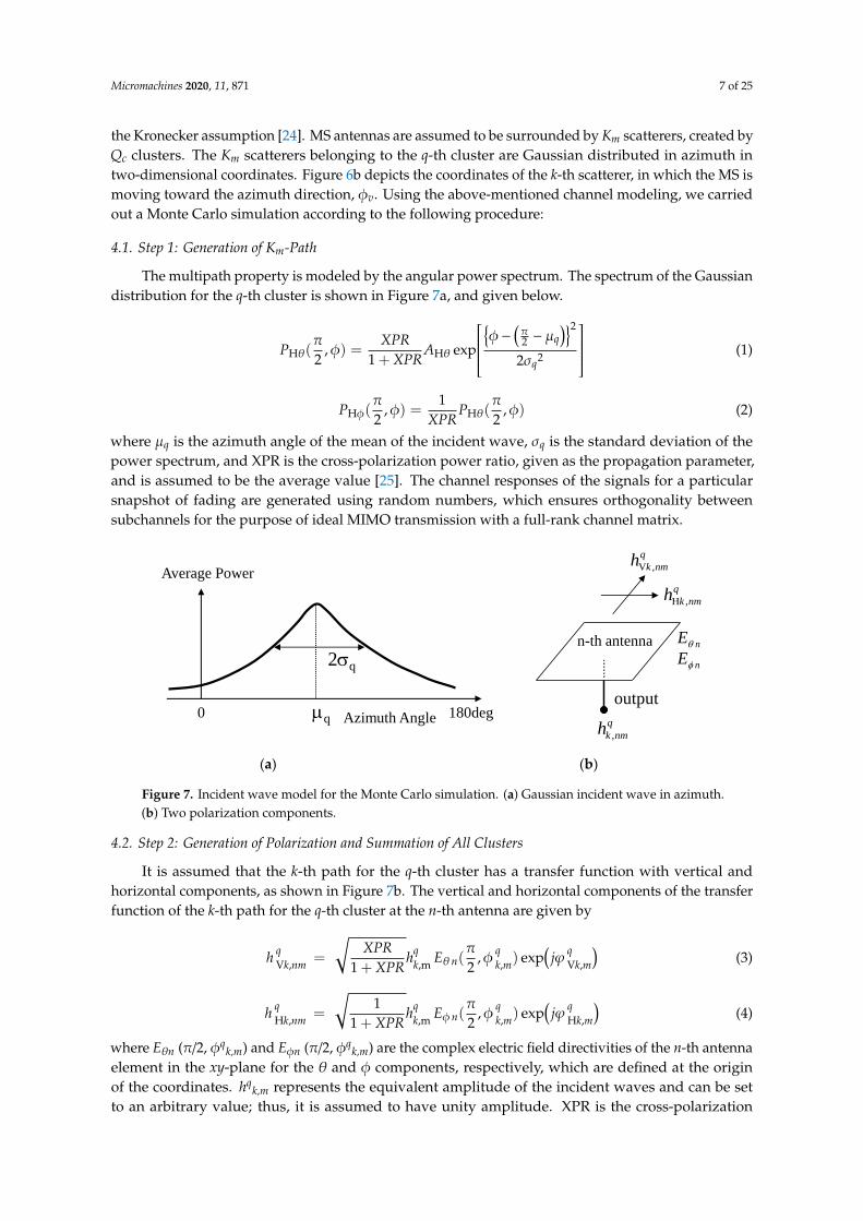
the Kronecker assumption [24]. MS antennas are assumed to be surrounded by Km scatterers, created byQc clusters. The Km scatterers belonging to the q-th cluster are Gaussian distributed in azimuth intwo-dimensional coordinates. Figure 6b depicts the coordinates of the k-th scatterer, in which the MS ismoving toward the azimuth direction, φv. Using the above-mentioned channel modeling, we carriedout a Monte Carlo simulation according to the following procedure:
4.1. Step 1: Generation of Km-Path
The multipath property is modeled by the angular power spectrum. The spectrum of the Gaussiandistribution for the q-th cluster is shown in Figure 7a, and given below.
PHθ(π2
,φ) =XPR
1 + XPRAHθ exp
{φ−
(π2 − µq
)}2
2σq2
(1)
PHφ(π2
,φ) =1
XPRPHθ(
π2
,φ) (2)
where µq is the azimuth angle of the mean of the incident wave, σq is the standard deviation of thepower spectrum, and XPR is the cross-polarization power ratio, given as the propagation parameter,and is assumed to be the average value [25]. The channel responses of the signals for a particularsnapshot of fading are generated using random numbers, which ensures orthogonality betweensubchannels for the purpose of ideal MIMO transmission with a full-rank channel matrix.
Micromachines 2020, 11, x 7 of 25
created by Qc clusters. The Km scatterers belonging to the q-th cluster are Gaussian distributed in
azimuth in two-dimensional coordinates. Figure 6b depicts the coordinates of the k-th scatterer, in
which the MS is moving toward the azimuth direction, ϕv. Using the above-mentioned channel
modeling, we carried out a Monte Carlo simulation according to the following procedure:
4.1. Step 1: Generation of Km-Path
The multipath property is modeled by the angular power spectrum. The spectrum of the
Gaussian distribution for the q-th cluster is shown in Figure 7a, and given below.
2
H H 2
2( , ) exp
2 1 2
q
q
XPRP A
XPRq q
p
p
=
(1)
H H
1( , ) ( , )
2 2P P
XPR q
p p = (2)
where µq is the azimuth angle of the mean of the incident wave, σq is the standard deviation of the
power spectrum, and XPR is the cross-polarization power ratio, given as the propagation parameter,
and is assumed to be the average value [25]. The channel responses of the signals for a particular
snapshot of fading are generated using random numbers, which ensures orthogonality between
subchannels for the purpose of ideal MIMO transmission with a full-rank channel matrix.
(a) (b)
Figure 7. Incident wave model for the Monte Carlo simulation. (a) Gaussian incident wave in azimuth.
(b) Two polarization components.
4.2. Step 2: Generation of Polarization and Summation of All Clusters
It is assumed that the k-th path for the q-th cluster has a transfer function with vertical and
horizontal components, as shown in Figure 7b. The vertical and horizontal components of the transfer
function of the k-th path for the q-th cluster at the n-th antenna are given by
V , ,m , V ,( , )exp1 2
q q q q
k nm k n k m k m
XPRh h E j
XPRq
p =
(3)
H , ,m , H ,
1( , )exp
1 2
q q q q
k nm k n k m k mh h E jXPR
p =
(4)
where Eθn (π/2, ϕqk,m) and Eϕn (π/2, ϕqk,m) are the complex electric field directivities of the n-th antenna
element in the xy-plane for the θ and ϕ components, respectively, which are defined at the origin of
the coordinates. hqk,m represents the equivalent amplitude of the incident waves and can be set to an
arbitrary value; thus, it is assumed to have unity amplitude. XPR is the cross-polarization power
Average Power
Azimuth Angle0 180degq
2q
,
q
k nmh
nEq
nE
V ,
q
k nmh
n-th antenna
H ,
q
k nmh
output
Figure 7. Incident wave model for the Monte Carlo simulation. (a) Gaussian incident wave in azimuth.(b) Two polarization components.
4.2. Step 2: Generation of Polarization and Summation of All Clusters
It is assumed that the k-th path for the q-th cluster has a transfer function with vertical andhorizontal components, as shown in Figure 7b. The vertical and horizontal components of the transferfunction of the k-th path for the q-th cluster at the n-th antenna are given by
h qVk,nm =
√XPR
1 + XPRhq
k,m Eθn(π2
,φ qk,m) exp
(jϕ q
Vk,m
)(3)
h qHk,nm =
√1
1 + XPRhq
k,m Eφn(π2
,φ qk,m) exp
(jϕ q
Hk,m
)(4)
where Eθn (π/2, φqk,m) and Eφn (π/2, φq
k,m) are the complex electric field directivities of the n-th antennaelement in the xy-plane for the θ and φ components, respectively, which are defined at the originof the coordinates. hq
k,m represents the equivalent amplitude of the incident waves and can be setto an arbitrary value; thus, it is assumed to have unity amplitude. XPR is the cross-polarization
Micromachines 2020, 11, 871 8 of 25
power ratio. The phases of the vertical and horizontal polarization components, ϕqVk,m and ϕq
Hk,m,are independent of each other, and are uniformly distributed from 0 to 2π. For each path, the twopolarization components are combined with reference to the schematic diagram shown in Figure 7b,as the complex sum of the vertical and horizontal components, and we have
h qk,nm = h q
Vk,nm + h qHk,nm (5)
where the transfer function of the k-th path is evaluated by summing all the cluster responses, and isgiven by
hk,nm =
Qc∑q=1
hqk,nm (6)
4.3. Step 3: Generation of the Resultant Channel Response
Using the transfer function represented by Equation (6), the resultant channel response at the n-thantenna is calculated using the equation
hnm =
Km∑k=1
hk,nm exp{
j2πdλ
cos(φ k,m − φ v)
}(7)
where λ is the wavelength in free space, and d is the distance traveled by a mobile station movingtoward the azimuth direction φv, as shown in Figure 6b. This scheme is applied repeatedly to generatethe following channel response matrix at the s-th snapshot
Hs = [hnm] =
h11 h12 · · · h1mh21 h22 · · · h2m
......
. . ....
hn1 hn2 · · · hNM
(8)
The distance traveled by the mobile station between two successive points, ∆d, in the simulationis changed according to the angular spread of the incident waves, because a narrow spread results in along fading period. For each value of d, fading is assumed to be quasi-static, i.e., the channel responseis kept constant.
The complex correlation coefficient between two channel responses is defined as
ρc =〈h1∗h2〉
√〈h1∗h1〉√〈h2∗h2〉
(9)
where h1 and h2 represent the two distinct channel responses in the matrix of Equation (8), and <X>
denotes the ensemble average of X where Y* represents the complex conjugate of Y. Using thisdefinition, the absolute value of the complex correlation coefficient can be obtained from
ρa =∣∣∣ρc
∣∣∣ (10)
Here, the absolute value of the complex correlation coefficient ρa in Equation (10) is used as ageneral description of the correlation behavior of the MIMO antenna performance throughout thispaper, as mentioned in Section 5.
4.4. Step 4: Evaluation of the Channel Capacity
The eigenvalues and eigenvectors are obtained using the following SVD (singular valuedecomposition) operation
Hs = UsDsVHs (11)
Micromachines 2020, 11, 871 9 of 25
Us = [er1, · · · , erL] (12)
Vs = [et1, · · · , etL] (13)
Ds = diag[√λ1, · · · ,
√λL
](14)
where L = min (N, M). Us and Vs are the singular vectors of the receiving (mobile station) andtransmitting (base station) antennas, respectively. Ds represents the singular values, where λidenotes the eigenvalue of the i-th subchannel for spatial multiplexing transmission in the MIMOsystem. Using these eigenvalues, the instantaneous channel capacity and its average value are finallyevaluated by
Cs =L∑
i=1
log2
(1 +
γλi
M
)(15)
C =1S
S∑s=1
Cs (s = 1 · · · S) (16)
where γ is the input SNR (signal-to-noise power ratio), defined as the SNR for each incident wavewhen an isotropic antenna is used for receiving the incident wave, permitting the performance of theantenna elements used in the MIMO array to be included in the simulation results.
5. Theoretical Investigation
5.1. Design of 4 × 4 MIMO Antenna
As described in Section 3, the 4 × 4 MIMO antenna depicted in Figure 3b is used as a basiccomponent module or a fundamental functional unit cell to construct the 32 × 32 MIMO antenna array.Hence, in the first step of our investigation, we considered the design of the 4 × 4 MIMO antenna [19].
Two of the eight antenna elements arranged in the circle form a subarray that receives a subchannelof the MIMO communication, where the number of subarrays in the 4 × 4 MIMO antenna is four.The radius of the circle, a, was set to 4.9 cm so that the distance between adjacent elements (d1 shownin Figure 3b) was a quarter-wavelength at 2 GHz. In this case, the directivity of Subarray1 is expectedto have a cardioid radiation pattern in the absence of mutual electromagnetic coupling betweenantenna elements.
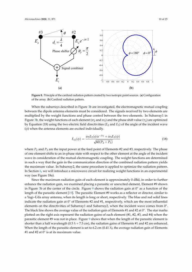
Figure 8 shows the fundamental principle of the cardioid radiation pattern created by two isotropicpoint sources corresponding to Elements #2 and #3 in Figure 3b, in which there is no electromagneticmutual coupling between the two sources. As shown in Figure 8a, the distance between the twosources is set to d1 = λ/4. Furthermore, the received signal from Element #2 is delayed by φp = π/2using a phase shifter. The total received signal, Et, is given by summing the received signals fromElements #2 and #3 using a signal combiner, and calculated from the equation
Et = Ea
[1 + exp
{jπ2(cosφ− 1)
}](17)
where φ represents the azimuthal angle defined in Figure 8. Ea denotes the amplitude of excitation ofeach element. Using this circuit topology shown in Figure 8a, an actual signal processing unit wasfabricated, as described in Section 6 (see Figure 18a).
Figure 8b illustrates the radiation pattern normalized to its peak value, calculated by the absolutevalue of Equation (17). As can be seen from Figure 8b, the radiation pattern directs its maximumtowards φ = 0◦ and exhibits a deep null towards φ = 180◦. Therefore, the array works as a phased arrayantenna that yields a strong radiation intensity in the direction of the line between the two sources.
Micromachines 2020, 11, 871 10 of 25Micromachines 2020, 11, x 10 of 25
(a) (b)
Figure 8. Principle of the cardioid radiation pattern created by two isotropic point sources. (a) Configuration of the array. (b) Cardioid radiation pattern.
When the subarrays described in Figure 3b are investigated, the electromagnetic mutual coupling between the dipole antenna elements must be considered. The signals received by two elements are multiplied by the weight functions and phase control between the two elements. In Subarray1 in Figure 3b, the weight functions of each element (w2 and w3) and the phase shift value (τ2) are optimized by Equation (18) using the two electric field directivities (E2 and E3) of the angle of the incident wave (ϕ) when the antenna elements are excited individually.
( ) ( ) ( )( )
22 2 3 3
12 360
j
s
w E e w EE
P P
τφ φφ
− +=
+ (18)
where P2 and P3 are the input power at the feed point of Elements #2 and #3, respectively. The phase of one element shifts to an in-phase state with respect to the other element at the angle of the incident wave in consideration of the mutual electromagnetic coupling. The weight functions are determined in such a way that the gain in the communication direction of the combined radiation pattern yields the maximum value. In Subarray2, the same procedure is applied to optimize the radiation pattern. In Section 6, we will introduce a microwave circuit for realizing weight functions in an experimental way (see Figure 18a).
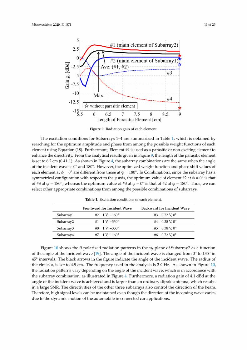
Since the maximum radiation gain of each element is approximately 0 dBd, in order to further enhance the radiation gain, we examined placing a parasitic or unexcited element, Element #9 shown in Figure 3b at the center of the circle. Figure 9 shows the radiation gain at 0° as a function of the length of the parasitic element [19]. The parasitic Element #9 works as a reflector or director, similar to a Yagi–Uda array antenna, when its length is long or short, respectively. The blue and red solid lines indicate the radiation gain at 0° of Elements #2 and #1, respectively, which are the most influential elements on the directivities of Subarray1 and Subarray2, when the incident wave comes from 0°. The black line shows the average value of the radiation gain of Elements #1 and #2 at 0°. The star marks plotted on the right axis represent the radiation gains of each element (#1, #2, #3, and #4) when the parasitic element #9 was not in place. Figure 9 shows that when the length of the parasitic element is shorter than a half wavelength (0.5 λ = 7.5 cm), the radiation gains of Elements #1 and #2 are enhanced. When the length of the parasitic element is set to 6.2 cm (0.41 λ), the average radiation gain of Elements #1 and #2 at 0° is at its maximum value.
-1 -0.8 -0.6 -0.4 -0.2 0 0.2 0.4 0.6 0.8 1-1
-0.8
-0.6
-0.4
-0.2
0
0.2
0.4
0.6
0.8
1
+
#3 #2
1 4d λ=
2pπφ =
tE
0φ = °180φ = ° φ
φ
Phase shifter
Signal combiner
aE /2jaE e π−
Figure 8. Principle of the cardioid radiation pattern created by two isotropic point sources. (a) Configurationof the array. (b) Cardioid radiation pattern.
When the subarrays described in Figure 3b are investigated, the electromagnetic mutual couplingbetween the dipole antenna elements must be considered. The signals received by two elements aremultiplied by the weight functions and phase control between the two elements. In Subarray1 inFigure 3b, the weight functions of each element (w2 and w3) and the phase shift value (τ2) are optimizedby Equation (18) using the two electric field directivities (E2 and E3) of the angle of the incident wave(φ) when the antenna elements are excited individually.
Es1(φ) =w2E2(φ)e− jτ2 + w3E3(φ)√
60(P2 + P3)(18)
where P2 and P3 are the input power at the feed point of Elements #2 and #3, respectively. The phaseof one element shifts to an in-phase state with respect to the other element at the angle of the incidentwave in consideration of the mutual electromagnetic coupling. The weight functions are determinedin such a way that the gain in the communication direction of the combined radiation pattern yieldsthe maximum value. In Subarray2, the same procedure is applied to optimize the radiation pattern.In Section 6, we will introduce a microwave circuit for realizing weight functions in an experimentalway (see Figure 18a).
Since the maximum radiation gain of each element is approximately 0 dBd, in order to furtherenhance the radiation gain, we examined placing a parasitic or unexcited element, Element #9 shownin Figure 3b at the center of the circle. Figure 9 shows the radiation gain at 0◦ as a function of thelength of the parasitic element [19]. The parasitic Element #9 works as a reflector or director, similar toa Yagi–Uda array antenna, when its length is long or short, respectively. The blue and red solid linesindicate the radiation gain at 0◦ of Elements #2 and #1, respectively, which are the most influentialelements on the directivities of Subarray1 and Subarray2, when the incident wave comes from 0◦.The black line shows the average value of the radiation gain of Elements #1 and #2 at 0◦. The star marksplotted on the right axis represent the radiation gains of each element (#1, #2, #3, and #4) when theparasitic element #9 was not in place. Figure 9 shows that when the length of the parasitic element isshorter than a half wavelength (0.5 λ = 7.5 cm), the radiation gains of Elements #1 and #2 are enhanced.When the length of the parasitic element is set to 6.2 cm (0.41 λ), the average radiation gain of Elements#1 and #2 at 0◦ is at its maximum value.
Micromachines 2020, 11, 871 11 of 25Micromachines 2020, 11, x 11 of 25
Figure 9. Radiation gain of each element.
The excitation conditions for Subarrays 1–4 are summarized in Table 1, which is obtained by searching for the optimum amplitude and phase from among the possible weight functions of each element using Equation (18). Furthermore, Element #9 is used as a parasitic or non-exciting element to enhance the directivity. From the analytical results given in Figure 9, the length of the parasitic element is set to 6.2 cm (0.41 λ). As shown in Figure 4, the subarray combinations are the same when the angle of the incident wave is 0° and 180°. However, the optimized weight function and phase shift values of each element at ϕ = 0° are different from those at ϕ = 180°. In Combination1, since the subarray has a symmetrical configuration with respect to the y-axis, the optimum value of element #2 at ϕ = 0° is that of #3 at ϕ = 180°, whereas the optimum value of #3 at ϕ = 0° is that of #2 at ϕ = 180°. Thus, we can select other appropriate combinations from among the possible combinations of subarrays.
Table 1. Excitation conditions of each element
Frontward for Incident Wave
Backward for Incident Wave
Subarray1 #2 1 V, −160° #3 0.72 V, 0°
Subarray2 #1 1 V, −330° #4 0.38 V, 0°
Subarray3 #8 1 V, −330° #5 0.38 V, 0°
Subarray4 #7 1 V, −160° #6 0.72 V, 0°
Figure 10 shows the θ-polarized radiation patterns in the xy-plane of Subarray2 as a function of the angle of the incident wave [19]. The angle of the incident wave is changed from 0° to 135° in 45° intervals. The black arrows in the figure indicate the angle of the incident wave. The radius of the circle, a, is set to 4.9 cm. The frequency used in the analysis is 2 GHz. As shown in Figure 10, the radiation patterns vary depending on the angle of the incident wave, which is in accordance with the subarray combination, as illustrated in Figure 4. Furthermore, a radiation gain of 4.1 dBd at the angle of the incident wave is achieved and is larger than an ordinary dipole antenna, which results in a large SNR. The directivities of the other three subarrays also control the direction of the beam. Therefore, high signal levels can be maintained even though the direction of the incoming wave varies due to the dynamic motion of the automobile in connected car applications.
5.5 6 6.5 7 7.5 8 8.5 9-15
-12.5
-10
-7.5
-5
-2.5
0
2.5
5
Length of Parasitic Element [cm]
Gai
n g 0 [d
Bd]
#1 (main element of Subarray2)
#2 (main element of Subarray1)
#4
#3Ave. (#1, #2)
Max
without parasitic element
Gai
n g 0
[dBd
]
Figure 9. Radiation gain of each element.
The excitation conditions for Subarrays 1–4 are summarized in Table 1, which is obtained bysearching for the optimum amplitude and phase from among the possible weight functions of eachelement using Equation (18). Furthermore, Element #9 is used as a parasitic or non-exciting element toenhance the directivity. From the analytical results given in Figure 9, the length of the parasitic elementis set to 6.2 cm (0.41 λ). As shown in Figure 4, the subarray combinations are the same when the angleof the incident wave is 0◦ and 180◦. However, the optimized weight function and phase shift values ofeach element at φ = 0◦ are different from those at φ = 180◦. In Combination1, since the subarray has asymmetrical configuration with respect to the y-axis, the optimum value of element #2 at φ = 0◦ is thatof #3 at φ = 180◦, whereas the optimum value of #3 at φ = 0◦ is that of #2 at φ = 180◦. Thus, we canselect other appropriate combinations from among the possible combinations of subarrays.
Table 1. Excitation conditions of each element.
Frontward for Incident Wave Backward for Incident Wave
Subarray1 #2 1 V, −160◦ #3 0.72 V, 0◦
Subarray2 #1 1 V, −330◦ #4 0.38 V, 0◦
Subarray3 #8 1 V, −330◦ #5 0.38 V, 0◦
Subarray4 #7 1 V, −160◦ #6 0.72 V, 0◦
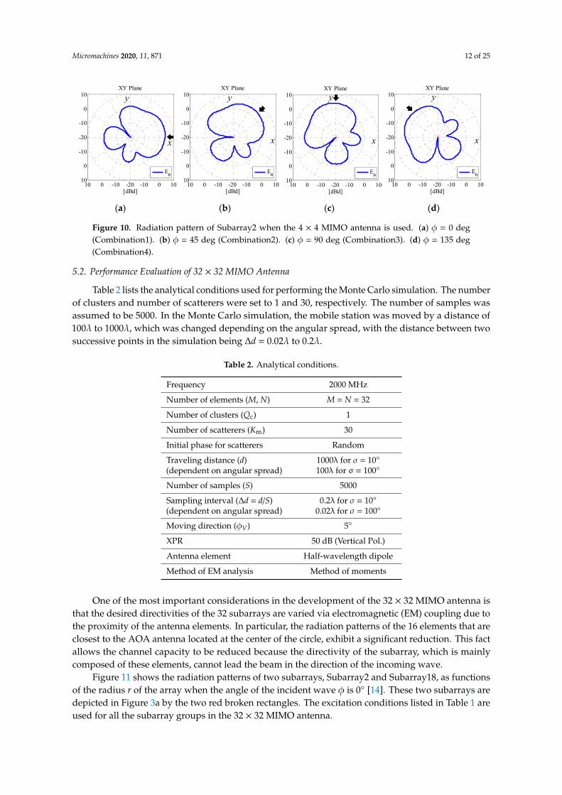
Figure 10 shows the θ-polarized radiation patterns in the xy-plane of Subarray2 as a functionof the angle of the incident wave [19]. The angle of the incident wave is changed from 0◦ to 135◦ in45◦ intervals. The black arrows in the figure indicate the angle of the incident wave. The radius ofthe circle, a, is set to 4.9 cm. The frequency used in the analysis is 2 GHz. As shown in Figure 10,the radiation patterns vary depending on the angle of the incident wave, which is in accordance withthe subarray combination, as illustrated in Figure 4. Furthermore, a radiation gain of 4.1 dBd at theangle of the incident wave is achieved and is larger than an ordinary dipole antenna, which resultsin a large SNR. The directivities of the other three subarrays also control the direction of the beam.Therefore, high signal levels can be maintained even though the direction of the incoming wave variesdue to the dynamic motion of the automobile in connected car applications.
Micromachines 2020, 11, 871 12 of 25Micromachines 2020, 11, x 12 of 25
(a) (b) (c) (d)
Figure 10. Radiation pattern of Subarray2 when the 4 × 4 MIMO antenna is used. (a) ϕ = 0 deg (Combination1). (b) ϕ = 45 deg (Combination2). (c) ϕ = 90 deg (Combination3). (d) ϕ = 135 deg (Combination4).
5.2. Performance Evaluation of 32 × 32 MIMO Antenna
Table 2 lists the analytical conditions used for performing the Monte Carlo simulation. The number of clusters and number of scatterers were set to 1 and 30, respectively. The number of samples was assumed to be 5000. In the Monte Carlo simulation, the mobile station was moved by a distance of 100λ to 1000λ, which was changed depending on the angular spread, with the distance between two successive points in the simulation being Δd = 0.02λ to 0.2λ.
Table 2. Analytical conditions.
Frequency 2000 MHz Number of elements (M, N) M = N = 32 Number of clusters (Qc) 1 Number of scatterers (Km) 30 Initial phase for scatterers Random Traveling distance (d) (dependent on angular spread)
1000λ for σ = 10° 100λ for σ = 100°
Number of samples (S) 5000 Sampling interval (Δd = d/S) (dependent on angular spread)
0.2λ for σ = 10° 0.02λ for σ = 100°
Moving direction (ϕV) 5° XPR 50 dB (Vertical Pol.) Antenna element Half-wavelength dipole Method of EM analysis Method of moments
One of the most important considerations in the development of the 32 × 32 MIMO antenna is that the desired directivities of the 32 subarrays are varied via electromagnetic (EM) coupling due to the proximity of the antenna elements. In particular, the radiation patterns of the 16 elements that are closest to the AOA antenna located at the center of the circle, exhibit a significant reduction. This fact allows the channel capacity to be reduced because the directivity of the subarray, which is mainly composed of these elements, cannot lead the beam in the direction of the incoming wave.
Figure 11 shows the radiation patterns of two subarrays, Subarray2 and Subarray18, as functions of the radius r of the array when the angle of the incident wave ϕ is 0° [14]. These two subarrays are depicted in Figure 3a by the two red broken rectangles. The excitation conditions listed in Table 1 are used for all the subarray groups in the 32 × 32 MIMO antenna.
10 0 -10 -20 -10 0 1010
0
-10
-20
-10
0
10
[dBd]
XY Plane
Eθ
10 0 -10 -20 -10 0 1010
0
-10
-20
-10
0
10
[dBd]
XY Plane
Eθ
10 0 -10 -20 -10 0 1010
0
-10
-20
-10
0
10
[dBd]
XY Plane
Eθ
10 0 -10 -20 -10 0 1010
0
-10
-20
-10
0
10
[dBd]
XY Plane
Eθ
x
y
x
y
x
y
x
y
Figure 10. Radiation pattern of Subarray2 when the 4 × 4 MIMO antenna is used. (a) φ = 0 deg(Combination1). (b) φ = 45 deg (Combination2). (c) φ = 90 deg (Combination3). (d) φ = 135 deg(Combination4).
5.2. Performance Evaluation of 32 × 32 MIMO Antenna
Table 2 lists the analytical conditions used for performing the Monte Carlo simulation. The numberof clusters and number of scatterers were set to 1 and 30, respectively. The number of samples wasassumed to be 5000. In the Monte Carlo simulation, the mobile station was moved by a distance of100λ to 1000λ, which was changed depending on the angular spread, with the distance between twosuccessive points in the simulation being ∆d = 0.02λ to 0.2λ.
Table 2. Analytical conditions.
Frequency 2000 MHz
Number of elements (M, N) M = N = 32
Number of clusters (Qc) 1
Number of scatterers (Km) 30
Initial phase for scatterers Random
Traveling distance (d)(dependent on angular spread)
1000λ for σ = 10◦
100λ for σ = 100◦
Number of samples (S) 5000
Sampling interval (∆d = d/S)(dependent on angular spread)
0.2λ for σ = 10◦
0.02λ for σ = 100◦
Moving direction (φV) 5◦
XPR 50 dB (Vertical Pol.)
Antenna element Half-wavelength dipole
Method of EM analysis Method of moments
One of the most important considerations in the development of the 32 × 32 MIMO antenna isthat the desired directivities of the 32 subarrays are varied via electromagnetic (EM) coupling due tothe proximity of the antenna elements. In particular, the radiation patterns of the 16 elements that areclosest to the AOA antenna located at the center of the circle, exhibit a significant reduction. This factallows the channel capacity to be reduced because the directivity of the subarray, which is mainlycomposed of these elements, cannot lead the beam in the direction of the incoming wave.
Figure 11 shows the radiation patterns of two subarrays, Subarray2 and Subarray18, as functionsof the radius r of the array when the angle of the incident wave φ is 0◦ [14]. These two subarrays aredepicted in Figure 3a by the two red broken rectangles. The excitation conditions listed in Table 1 areused for all the subarray groups in the 32 × 32 MIMO antenna.

Micromachines 2020, 11, 871 13 of 25Micromachines 2020, 11, x 13 of 25
(a) (b)
Figure 11. Radiation patterns of Subarray2 and Subarray18 when the 32 × 32 MIMO antenna is used. (a) Subarray2. (b) Subarray18.
In Figure 11, the black and red solid lines indicate the radiation patterns at r = 30 cm and r = 15 cm, respectively. The blue broken line indicates the radiation pattern of the 4 × 4 MIMO array without EM coupling caused by other 4 × 4 MIMO arrays [19]. The black arrows in the figure show the angle of the incident wave. As shown in Figure 11, the radiation gains at an incident-wave angle of 0° for Subarray2 is constant regardless of the radius r, while the radiation gain at ϕ = 0° for the 32 × 32 MIMO array agrees well with that for the 4 × 4 MIMO array. This is because the radiation beam from Subarray2 is directed to the outside of the whole antenna system and is less affected by the EM coupling caused by the other 4 × 4 MIMO arrays.
In contrast, the radiation gains at ϕ = 0° for Subarray18 are significantly degraded by the EM coupling when r = 15 cm. This is due to the fact that Subarray18 directs its radiation beam toward the AOA antenna and is significantly affected by EM coupling with the AOA antenna. However, the radiation gain at r = 30 cm is improved considerably and is close to that of the 4 × 4 MIMO array. These results show that the radiation gain at the angle of the incident wave increases with increasing radius due to smaller EM coupling.
The final target of our study is to obtain transmission rates greater than a gigabit to ensure the success of these arrays in upcoming connected car systems. Hence, to investigate the optimum radius for this purpose, the channel capacity is calculated through Monte Carlo simulations, with a single cluster Gaussian spectrum coming from azimuth angle ϕ, as depicted in Figure 3b.
Figure 12 shows the average channel capacity, calculated from Equation (16), as a function of the radius r at 2 GHz [14]. The black and red curves correspond to incident-wave angles ϕ of 0° and 45°. Half-wavelength dipole antennas are used for the 64 elements. The radius of the 4 × 4 MIMO antenna a is set to 4.9 cm. The cross-polarization power ratio, XPR, is set to 50 dB, which is equivalent to a vertically polarized propagation environment. The standard deviation of the incident wave σ (σ1 for the cluster1 in Figure 7a) is set to 30°. The SNR of the incident wave is set to 30 dB.
Figure 12 shows that a channel capacity of over 220 bits/s/Hz is achieved when r is greater than 30 cm, which is equivalent to 22 Gbps for a bandwidth of 100 MHz. The channel capacity increases by 52 bits/s/Hz when r = 30 cm, compared with the case where r = 15 cm. Furthermore, the channel capacity remains constant after r = 30 cm, meaning that, considering the size of the array, r = 30 cm is one of the best possible solutions for obtaining the maximum channel capacity with an array of limited size. Note that the black and red curves at angles of 0° and 45° closely overlap. This is due to the fact that, as described in Figure 4, the 32 × 32 MIMO array uses different combinations of subarrays, Combination1 and Combination2, at ϕ = 0° and 45°, which enables the radiation gain in these directions to be enhanced with equal intensity. Consequently, we have the same level of channel
10 0 -10 -20 -10 0 10 10
0
-10
-20
-10
0
10
[dBd]
10 0 -10 -20 -10 0 1010
0
-10
-20
-10
0
10
[dBd]
r = 30cmr = 15cm4 4MIMO
r = 30cmr = 15cm4 4MIMO
x
y
x
y
Figure 11. Radiation patterns of Subarray2 and Subarray18 when the 32 × 32 MIMO antenna is used.(a) Subarray2. (b) Subarray18.
In Figure 11, the black and red solid lines indicate the radiation patterns at r = 30 cm and r = 15 cm,respectively. The blue broken line indicates the radiation pattern of the 4 × 4 MIMO array without EMcoupling caused by other 4 × 4 MIMO arrays [19]. The black arrows in the figure show the angle of theincident wave. As shown in Figure 11, the radiation gains at an incident-wave angle of 0◦ for Subarray2is constant regardless of the radius r, while the radiation gain at φ = 0◦ for the 32 × 32 MIMO arrayagrees well with that for the 4 × 4 MIMO array. This is because the radiation beam from Subarray2 isdirected to the outside of the whole antenna system and is less affected by the EM coupling caused bythe other 4 × 4 MIMO arrays.
In contrast, the radiation gains at φ = 0◦ for Subarray18 are significantly degraded by the EMcoupling when r = 15 cm. This is due to the fact that Subarray18 directs its radiation beam towardthe AOA antenna and is significantly affected by EM coupling with the AOA antenna. However,the radiation gain at r = 30 cm is improved considerably and is close to that of the 4 × 4 MIMO array.These results show that the radiation gain at the angle of the incident wave increases with increasingradius due to smaller EM coupling.
The final target of our study is to obtain transmission rates greater than a gigabit to ensure thesuccess of these arrays in upcoming connected car systems. Hence, to investigate the optimum radiusfor this purpose, the channel capacity is calculated through Monte Carlo simulations, with a singlecluster Gaussian spectrum coming from azimuth angle φ, as depicted in Figure 3b.
Figure 12 shows the average channel capacity, calculated from Equation (16), as a function of theradius r at 2 GHz [14]. The black and red curves correspond to incident-wave angles φ of 0◦ and 45◦.Half-wavelength dipole antennas are used for the 64 elements. The radius of the 4 × 4 MIMO antennaa is set to 4.9 cm. The cross-polarization power ratio, XPR, is set to 50 dB, which is equivalent to avertically polarized propagation environment. The standard deviation of the incident wave σ (σ1 forthe cluster1 in Figure 7a) is set to 30◦. The SNR of the incident wave is set to 30 dB.
Figure 12 shows that a channel capacity of over 220 bits/s/Hz is achieved when r is greater than30 cm, which is equivalent to 22 Gbps for a bandwidth of 100 MHz. The channel capacity increasesby 52 bits/s/Hz when r = 30 cm, compared with the case where r = 15 cm. Furthermore, the channelcapacity remains constant after r = 30 cm, meaning that, considering the size of the array, r = 30 cm isone of the best possible solutions for obtaining the maximum channel capacity with an array of limitedsize. Note that the black and red curves at angles of 0◦ and 45◦ closely overlap. This is due to thefact that, as described in Figure 4, the 32 × 32 MIMO array uses different combinations of subarrays,Combination1 and Combination2, atφ = 0◦ and 45◦, which enables the radiation gain in these directionsto be enhanced with equal intensity. Consequently, we have the same level of channel capacity at these
Micromachines 2020, 11, 871 14 of 25
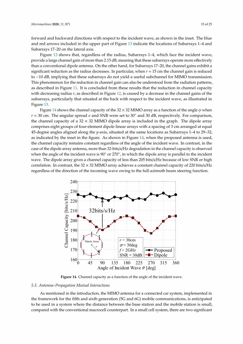
angles, which confirms that the beam steering function operates correctly, regardless of the size ofthe array.
Micromachines 2020, 11, x 14 of 25
capacity at these angles, which confirms that the beam steering function operates correctly, regardless of the size of the array.
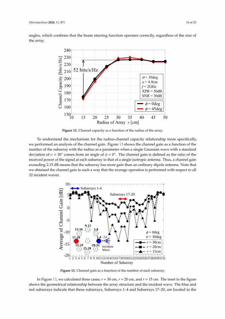
Figure 12. Channel capacity as a function of the radius of the array.
To understand the mechanism for the radius-channel capacity relationship more specifically, we performed an analysis of the channel gain. Figure 13 shows the channel gain as a function of the number of the subarray with the radius as a parameter when a single Gaussian wave with a standard deviation of σ = 30° comes from an angle of ϕ = 0°. The channel gain is defined as the ratio of the received power of the signal at each subarray to that of a single isotropic antenna. Thus, a channel gain exceeding 2.15 dB means that the subarray has more gain than an ordinary dipole antenna. Note that we obtained the channel gain in such a way that the average operation is performed with respect to all 32 incident waves.
Figure 13. Channel gain as a function of the number of each subarray.
In Figure 13, we calculated three cases; r = 30 cm, r = 20 cm, and r = 15 cm. The inset in the figure shows the geometrical relationship between the array structure and the incident wave. The blue and red subarrays indicate that these subarrays, Subarrays 1–4 and Subarrays 17–20, are located in the
10 15 20 25 30 35 40 45 50150160170180190200210220230240
Radius of Array r [cm]
Cha
nnel
Cap
acity
[bits
/s/H
z]
52 bits/s/Hzσ = 30dega = 4.9cmf = 2GHzXPR = 50dBSNR = 30dB
φ = 0degφ = 45deg
1 2 3 4 5 6 7 8 9 1011121314151617181920212223242526272829303132-20
-15
-10
-5
0
5
10
Number of Subarray
Ave
rage
of C
hann
el G
ain
[dB]
1-4
5-89-12
13-16
17-20
21-2425-28
29-32
2σ
Subarrays 1-4Subarrays 17-20
IncidentWave
r = 30cmr = 20cmr = 15cm
σ = 30degφ = 0deg
Aver
age
of C
hann
el G
ain
[dB]
-20
-15
-10
-5
0
5
10
Figure 12. Channel capacity as a function of the radius of the array.
To understand the mechanism for the radius-channel capacity relationship more specifically,we performed an analysis of the channel gain. Figure 13 shows the channel gain as a function of thenumber of the subarray with the radius as a parameter when a single Gaussian wave with a standarddeviation of σ = 30◦ comes from an angle of φ = 0◦. The channel gain is defined as the ratio of thereceived power of the signal at each subarray to that of a single isotropic antenna. Thus, a channel gainexceeding 2.15 dB means that the subarray has more gain than an ordinary dipole antenna. Note thatwe obtained the channel gain in such a way that the average operation is performed with respect to all32 incident waves.
Micromachines 2020, 11, x 14 of 25
capacity at these angles, which confirms that the beam steering function operates correctly, regardless
of the size of the array.
Figure 12. Channel capacity as a function of the radius of the array.
To understand the mechanism for the radius-channel capacity relationship more specifically, we
performed an analysis of the channel gain. Figure 13 shows the channel gain as a function of the
number of the subarray with the radius as a parameter when a single Gaussian wave with a standard
deviation of σ = 30° comes from an angle of ϕ = 0°. The channel gain is defined as the ratio of the
received power of the signal at each subarray to that of a single isotropic antenna. Thus, a channel
gain exceeding 2.15 dB means that the subarray has more gain than an ordinary dipole antenna. Note
that we obtained the channel gain in such a way that the average operation is performed with respect
to all 32 incident waves.
Figure 13. Channel gain as a function of the number of each subarray.
In Figure 13, we calculated three cases; r = 30 cm, r = 20 cm, and r = 15 cm. The inset in the figure
shows the geometrical relationship between the array structure and the incident wave. The blue and
red subarrays indicate that these subarrays, Subarrays 1–4 and Subarrays 17–20, are located in the
10 15 20 25 30 35 40 45 50150
160
170
180
190
200
210
220
230
240
Radius of Array r [cm]
Ch
ann
el
Capacit
y [
bit
s/s/
Hz]
52 bits/s/Hz
= 30deg
a = 4.9cm
f = 2GHz
XPR = 50dB
SNR = 30dB
= 0deg
= 45deg
1 2 3 4 5 6 7 8 9 1011121314151617181920212223242526272829303132-20
-15
-10
-5
0
5
10
Number of Subarray
Av
era
ge o
f C
han
nel
Gain
[d
B]
1-4
5-8
9-12
13-16
17-20
21-2425-28
29-32
2
Subarrays 1-4
Subarrays 17-20
IncidentWave
r = 30cm
r = 20cm
r = 15cm
= 30deg
= 0deg
Av
erag
e o
f C
han
nel
Gai
n [
dB
]
-20
-15
-10
-5
0
5
10
Figure 13. Channel gain as a function of the number of each subarray.
In Figure 13, we calculated three cases; r = 30 cm, r = 20 cm, and r = 15 cm. The inset in the figureshows the geometrical relationship between the array structure and the incident wave. The blue andred subarrays indicate that these subarrays, Subarrays 1–4 and Subarrays 17–20, are located in the
Micromachines 2020, 11, 871 15 of 25
forward and backward directions with respect to the incident wave, as shown in the inset. The blueand red arrows included in the upper part of Figure 13 indicate the locations of Subarrays 1–4 andSubarrays 17–20 on the lateral axis.
Figure 13 shows that, regardless of the radius, Subarrays 1–4, which face the incident wave,provide a large channel gain of more than 2.15 dB, meaning that these subarrays operate more effectivelythan a conventional dipole antenna. On the other hand, for Subarrays 17–20, the channel gains exhibit asignificant reduction as the radius decreases. In particular, when r = 15 cm the channel gain is reducedto −10 dB, implying that these subarrays do not yield a useful subchannel for MIMO transmission.This phenomenon for the reduction in channel gain can also be understood from the radiation patterns,as described in Figure 11. It is concluded from these results that the reduction in channel capacitywith decreasing radius r, as described in Figure 12, is caused by a decrease in the channel gains of thesubarrays, particularly that situated at the back with respect to the incident wave, as illustrated inFigure 13.
Figure 14 shows the channel capacity of the 32 × 32 MIMO array as a function of the angle φwhenr = 30 cm. The angular spread σ and SNR were set to 30◦ and 30 dB, respectively. For comparison,the channel capacity of a 32 × 32 MIMO dipole array is included in the graph. The dipole arraycomprises eight groups of four-element dipole linear arrays with a spacing of 3 cm arranged at equal45-degree angles aligned along the y-axis, situated at the same locations as Subarrays 1–4 to 29–32,as indicated by the inset in the figure. As shown in Figure 14, when the proposed antenna is used,the channel capacity remains constant regardless of the angle of the incident wave. In contrast, in thecase of the dipole array antenna, more than 32-bits/s/Hz degradation in the channel capacity is observedwhen the angle of the incident wave is 90◦ or 270◦, in which the dipole array is parallel to the incidentwave. The dipole array gives a channel capacity of less than 205 bits/s/Hz because of low SNR or highcorrelation. In contrast, the 32 × 32 MIMO array achieves a constant channel capacity of 220 bits/s/Hzregardless of the direction of the incoming wave owing to the full-azimuth beam steering function.
Micromachines 2020, 11, x 15 of 25
forward and backward directions with respect to the incident wave, as shown in the inset. The blue and red arrows included in the upper part of Figure 13 indicate the locations of Subarrays 1–4 and Subarrays 17–20 on the lateral axis.
Figure 13 shows that, regardless of the radius, Subarrays 1–4, which face the incident wave, provide a large channel gain of more than 2.15 dB, meaning that these subarrays operate more effectively than a conventional dipole antenna. On the other hand, for Subarrays 17–20, the channel gains exhibit a significant reduction as the radius decreases. In particular, when r = 15 cm the channel gain is reduced to −10 dB, implying that these subarrays do not yield a useful subchannel for MIMO transmission. This phenomenon for the reduction in channel gain can also be understood from the radiation patterns, as described in Figure 11. It is concluded from these results that the reduction in channel capacity with decreasing radius r, as described in Figure 12, is caused by a decrease in the channel gains of the subarrays, particularly that situated at the back with respect to the incident wave, as illustrated in Figure 13.
Figure 14 shows the channel capacity of the 32 × 32 MIMO array as a function of the angle ϕ when r = 30 cm. The angular spread σ and SNR were set to 30° and 30 dB, respectively. For comparison, the channel capacity of a 32 × 32 MIMO dipole array is included in the graph. The dipole array comprises eight groups of four-element dipole linear arrays with a spacing of 3 cm arranged at equal 45-degree angles aligned along the y-axis, situated at the same locations as Subarrays 1–4 to 29–32, as indicated by the inset in the figure. As shown in Figure 14, when the proposed antenna is used, the channel capacity remains constant regardless of the angle of the incident wave. In contrast, in the case of the dipole array antenna, more than 32-bits/s/Hz degradation in the channel capacity is observed when the angle of the incident wave is 90° or 270°, in which the dipole array is parallel to the incident wave. The dipole array gives a channel capacity of less than 205 bits/s/Hz because of low SNR or high correlation. In contrast, the 32 × 32 MIMO array achieves a constant channel capacity of 220 bits/s/Hz regardless of the direction of the incoming wave owing to the full-azimuth beam steering function.
Figure 14. Channel capacity as a function of the angle of the incident wave.
5.3. Antenna–Propagation Mutual Interactions
As mentioned in the introduction, the MIMO antenna for a connected car system, implemented in the framework for the fifth and sixth generation (5G and 6G) mobile communications, is anticipated to be used in a system where the distance between the base station and the mobile station is small, compared with the conventional macrocell counterpart. In a small cell system, there are two
0 45 90 135 180 225 270 315 360160
170
180
190
200
210
220
230
240
Angle of Incident Wave φ [deg]
Cha
nnel
Cap
acity
[bits
/s/H
z]
r = 30cmσ = 30degf = 2GHzSNR = 30dB
ProposedDipole
32bits/s/Hz
φ
rDipole Array
Figure 14. Channel capacity as a function of the angle of the incident wave.
5.3. Antenna–Propagation Mutual Interactions
As mentioned in the introduction, the MIMO antenna for a connected car system, implemented inthe framework for the fifth and sixth generation (5G and 6G) mobile communications, is anticipatedto be used in a system where the distance between the base station and the mobile station is small,compared with the conventional macrocell counterpart. In a small cell system, there are two significant
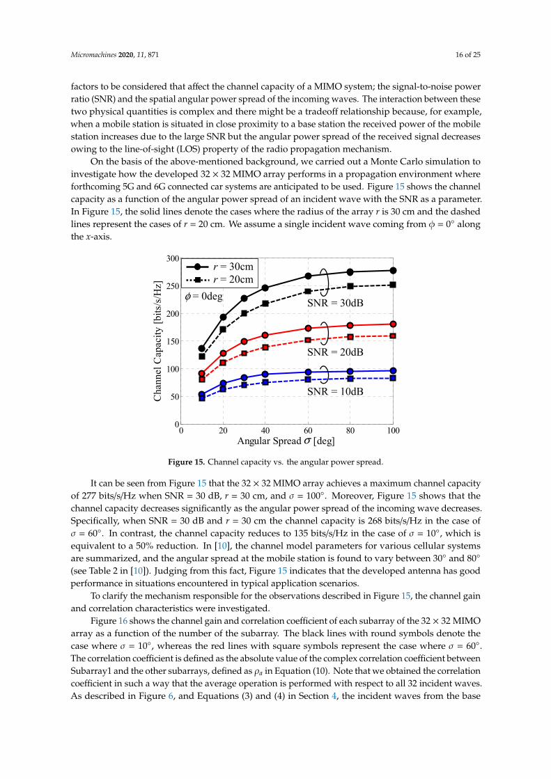
Micromachines 2020, 11, 871 16 of 25
factors to be considered that affect the channel capacity of a MIMO system; the signal-to-noise powerratio (SNR) and the spatial angular power spread of the incoming waves. The interaction between thesetwo physical quantities is complex and there might be a tradeoff relationship because, for example,when a mobile station is situated in close proximity to a base station the received power of the mobilestation increases due to the large SNR but the angular power spread of the received signal decreasesowing to the line-of-sight (LOS) property of the radio propagation mechanism.
On the basis of the above-mentioned background, we carried out a Monte Carlo simulation toinvestigate how the developed 32 × 32 MIMO array performs in a propagation environment whereforthcoming 5G and 6G connected car systems are anticipated to be used. Figure 15 shows the channelcapacity as a function of the angular power spread of an incident wave with the SNR as a parameter.In Figure 15, the solid lines denote the cases where the radius of the array r is 30 cm and the dashedlines represent the cases of r = 20 cm. We assume a single incident wave coming from φ = 0◦ alongthe x-axis.
Micromachines 2020, 11, x 16 of 25
significant factors to be considered that affect the channel capacity of a MIMO system; the signal-to-noise power ratio (SNR) and the spatial angular power spread of the incoming waves. The interaction between these two physical quantities is complex and there might be a tradeoff relationship because, for example, when a mobile station is situated in close proximity to a base station the received power of the mobile station increases due to the large SNR but the angular power spread of the received signal decreases owing to the line-of-sight (LOS) property of the radio propagation mechanism.
On the basis of the above-mentioned background, we carried out a Monte Carlo simulation to investigate how the developed 32 × 32 MIMO array performs in a propagation environment where forthcoming 5G and 6G connected car systems are anticipated to be used. Figure 15 shows the channel capacity as a function of the angular power spread of an incident wave with the SNR as a parameter. In Figure 15, the solid lines denote the cases where the radius of the array r is 30 cm and the dashed lines represent the cases of r = 20 cm. We assume a single incident wave coming from ϕ = 0° along the x-axis.
Figure 15. Channel capacity vs. the angular power spread.
It can be seen from Figure 15 that the 32 × 32 MIMO array achieves a maximum channel capacity of 277 bits/s/Hz when SNR = 30 dB, r = 30 cm, and σ = 100°. Moreover, Figure 15 shows that the channel capacity decreases significantly as the angular power spread of the incoming wave decreases. Specifically, when SNR = 30 dB and r = 30 cm the channel capacity is 268 bits/s/Hz in the case of σ = 60°. In contrast, the channel capacity reduces to 135 bits/s/Hz in the case of σ = 10°, which is equivalent to a 50% reduction. In [10], the channel model parameters for various cellular systems are summarized, and the angular spread at the mobile station is found to vary between 30° and 80° (see Table 2 in [10]). Judging from this fact, Figure 15 indicates that the developed antenna has good performance in situations encountered in typical application scenarios.
To clarify the mechanism responsible for the observations described in Figure 15, the channel gain and correlation characteristics were investigated.
Figure 16 shows the channel gain and correlation coefficient of each subarray of the 32 × 32 MIMO array as a function of the number of the subarray. The black lines with round symbols denote the case where σ = 10°, whereas the red lines with square symbols represent the case where σ = 60°. The correlation coefficient is defined as the absolute value of the complex correlation coefficient between Subarray1 and the other subarrays, defined as ρa in Equation (10). Note that we obtained the correlation coefficient in such a way that the average operation is performed with respect to all 32 incident waves. As described in Figure 6, and Equations (3) and (4) in Section 4, the incident waves from the base station are assumed to be plane waves, i.e., far-field assumption, and thus the channel
0 20 40 60 80 1000
50
100
150
200
250
300
Angular Spread σ [deg]
Cha
nnel
Cap
acity
[bits
/s/H
z]
SNR = 30dB
SNR = 20dB
SNR = 10dB
φ = 0degr = 20cmr = 30cm
σ
Figure 15. Channel capacity vs. the angular power spread.
It can be seen from Figure 15 that the 32 × 32 MIMO array achieves a maximum channel capacityof 277 bits/s/Hz when SNR = 30 dB, r = 30 cm, and σ = 100◦. Moreover, Figure 15 shows that thechannel capacity decreases significantly as the angular power spread of the incoming wave decreases.Specifically, when SNR = 30 dB and r = 30 cm the channel capacity is 268 bits/s/Hz in the case ofσ = 60◦. In contrast, the channel capacity reduces to 135 bits/s/Hz in the case of σ = 10◦, which isequivalent to a 50% reduction. In [10], the channel model parameters for various cellular systemsare summarized, and the angular spread at the mobile station is found to vary between 30◦ and 80◦
(see Table 2 in [10]). Judging from this fact, Figure 15 indicates that the developed antenna has goodperformance in situations encountered in typical application scenarios.
To clarify the mechanism responsible for the observations described in Figure 15, the channel gainand correlation characteristics were investigated.
Figure 16 shows the channel gain and correlation coefficient of each subarray of the 32 × 32 MIMOarray as a function of the number of the subarray. The black lines with round symbols denote thecase where σ = 10◦, whereas the red lines with square symbols represent the case where σ = 60◦.The correlation coefficient is defined as the absolute value of the complex correlation coefficient betweenSubarray1 and the other subarrays, defined as ρa in Equation (10). Note that we obtained the correlationcoefficient in such a way that the average operation is performed with respect to all 32 incident waves.As described in Figure 6, and Equations (3) and (4) in Section 4, the incident waves from the base
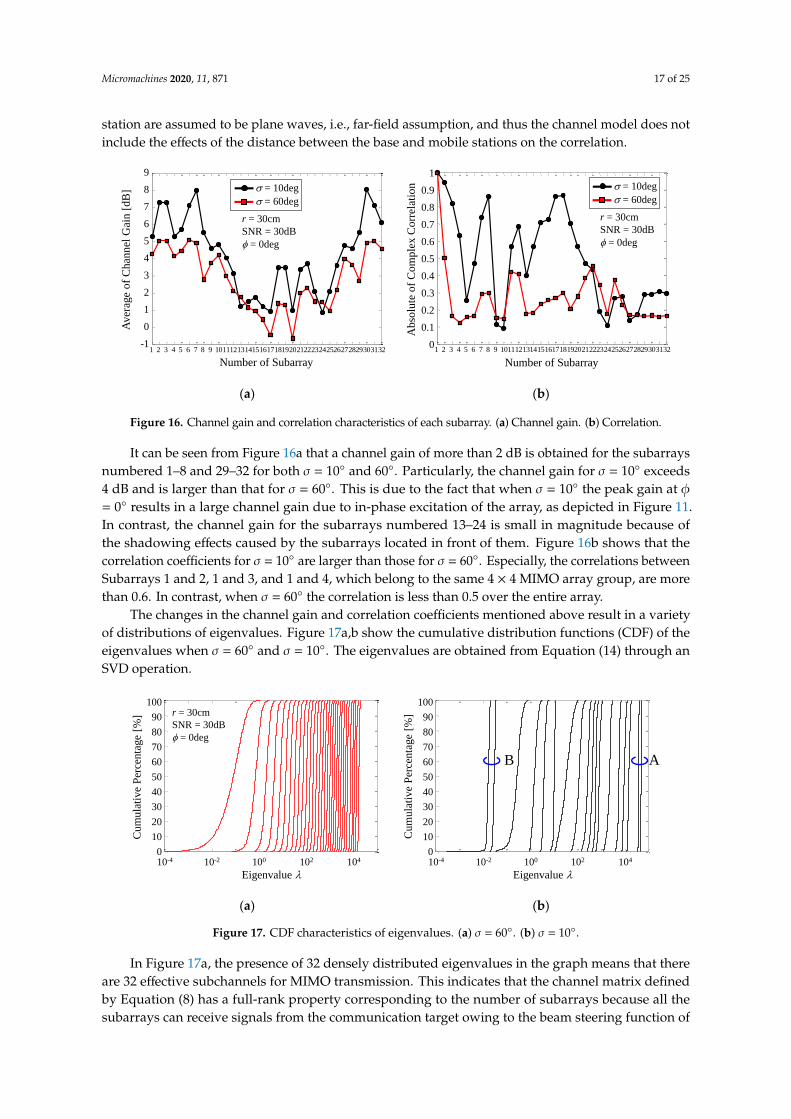
Micromachines 2020, 11, 871 17 of 25
station are assumed to be plane waves, i.e., far-field assumption, and thus the channel model does notinclude the effects of the distance between the base and mobile stations on the correlation.
Micromachines 2020, 11, x 17 of 25
model does not include the effects of the distance between the base and mobile stations on the
correlation.
It can be seen from Figure 16a that a channel gain of more than 2 dB is obtained for the subarrays
numbered 1–8 and 29–32 for both σ = 10° and 60°. Particularly, the channel gain for σ = 10° exceeds 4
dB and is larger than that for σ = 60°. This is due to the fact that when σ = 10° the peak gain at ϕ = 0°
results in a large channel gain due to in-phase excitation of the array, as depicted in Figure 11. In
contrast, the channel gain for the subarrays numbered 13–24 is small in magnitude because of the
shadowing effects caused by the subarrays located in front of them. Figure 16b shows that the
correlation coefficients for σ = 10° are larger than those for σ = 60°. Especially, the correlations between
Subarrays 1 and 2, 1 and 3, and 1 and 4, which belong to the same 4 × 4 MIMO array group, are more
than 0.6. In contrast, when σ = 60° the correlation is less than 0.5 over the entire array.
(a) (b)
Figure 16. Channel gain and correlation characteristics of each subarray. (a) Channel gain. (b)
Correlation.
The changes in the channel gain and correlation coefficients mentioned above result in a variety
of distributions of eigenvalues. Figure 17a,b show the cumulative distribution functions (CDF) of the
eigenvalues when σ = 60° and σ = 10°. The eigenvalues are obtained from Equation (14) through an
SVD operation.
In Figure 17a, the presence of 32 densely distributed eigenvalues in the graph means that there
are 32 effective subchannels for MIMO transmission. This indicates that the channel matrix defined
by Equation (8) has a full-rank property corresponding to the number of subarrays because all the
subarrays can receive signals from the communication target owing to the beam steering function of
the proposed antenna. This feature is quite different from a conventional circular array antenna with
a number of patch antennas arranged in a cylindrical manner [7,8], as described in the introduction.
Consequently, the developed antenna operates normally and effectively as a 32-element MIMO array
antenna.
In contrast, the sparsely distributed 18 eigenvalues, shown in Figure 17b, indicate that the
developed array works as a MIMO antenna with a small number of elements. More specifically, a
large channel gain in the case of σ = 10° provides large first and second eigenvalues, as indicated by
the symbol “A” on the right side of Figure 17b. Moreover, a high correlation coefficient for σ = 10°
creates small eigenvalues distributed on the left side of Figure 17b, as indicated by the symbol “B”.
Eventually, when σ = 10° these two observations result in a small channel capacity, as described in
Figure 15.
1 2 3 4 5 6 7 8 9 1011121314151617181920212223242526272829303132
1 2 3 4 5 6 7 8 9 1011121314151617181920212223242526272829303132
Av
erag
e o
f C
han
nel
Gai
n [
dB
]
Ab
solu
te o
f C
om
ple
x C
orr
elat
ion
Number of Subarray
9
8
7
6
5
4
3
2
1
0
-1
1
0.9
0.8
0.7
0.6
0.5
0.4
0.3
0.2
0.1
0
Number of Subarray
= 10deg
= 60deg
r = 30cm
SNR = 30dB
= 0deg
= 10deg
= 60deg
r = 30cm
SNR = 30dB
= 0deg
Figure 16. Channel gain and correlation characteristics of each subarray. (a) Channel gain. (b) Correlation.
It can be seen from Figure 16a that a channel gain of more than 2 dB is obtained for the subarraysnumbered 1–8 and 29–32 for both σ = 10◦ and 60◦. Particularly, the channel gain for σ = 10◦ exceeds4 dB and is larger than that for σ = 60◦. This is due to the fact that when σ = 10◦ the peak gain at φ= 0◦ results in a large channel gain due to in-phase excitation of the array, as depicted in Figure 11.In contrast, the channel gain for the subarrays numbered 13–24 is small in magnitude because ofthe shadowing effects caused by the subarrays located in front of them. Figure 16b shows that thecorrelation coefficients for σ = 10◦ are larger than those for σ = 60◦. Especially, the correlations betweenSubarrays 1 and 2, 1 and 3, and 1 and 4, which belong to the same 4 × 4 MIMO array group, are morethan 0.6. In contrast, when σ = 60◦ the correlation is less than 0.5 over the entire array.
The changes in the channel gain and correlation coefficients mentioned above result in a varietyof distributions of eigenvalues. Figure 17a,b show the cumulative distribution functions (CDF) of theeigenvalues when σ = 60◦ and σ = 10◦. The eigenvalues are obtained from Equation (14) through anSVD operation.
Micromachines 2020, 11, x 18 of 25
(a) (b)
Figure 17. CDF characteristics of eigenvalues. (a) σ = 60°. (b) σ = 10°.
From the extensive analytical investigations performed in this paper, we conclude that a
remarkably high channel capacity of more than 200 bits/s/Hz achieved by the beam steering 32 × 32
MIMO array—as depicted in Figures 12, 14, and 15—can be attributed to two significant factors; the
improved directivity due to in-phase excitation of the array and the low correlation between
subarrays caused by the orthogonal alignment of the array with respect to the incident waves.
6. Experimental Verification
To confirm the validity of the proposed antenna, this section presents experiments carried out
to evaluate the 4 × 4 and 32 × 32 MIMO arrays. We performed two types of measurements; radiation
pattern measurements in an anechoic chamber and over-the-air (OTA) testing using a two-
dimensional fading emulator in a cluster propagation environment [26].
6.1. Impedance and Radiation Measurements
Figure 18 shows the setup for measuring the radiation pattern of a 4 × 4 MIMO array in an
anechoic chamber [15]. The signal processing unit was designed using the circuit topology depicted
in Figure 8a, including a phase shifter and a signal combiner. Figure 18a shows a fabricated
microwave circuit for the weight functions of Subarry2 (w1 and w4) using a double-sided printed
circuit board with a thickness of 1 mm and a relative permittivity of 4.2 (FR4). The phase shift of the
received signal for each element was realized using different lengths of microstrip transmission lines.
The 30° phase difference between #1 and #4 is equivalent to a difference in length of 7.6 mm. The
phase difference of the produced network was 34°, indicating that the phase difference was achieved.
Furthermore, to get the correct weight function, the difference in power loss between the microstrip
lines, which was 0.21 dB, was considered.
(a) (b)
Figure 18. Radiation pattern measurement setup of a 4 × 4 MIMO array in an anechoic chamber. (a)
Fabricated microwave circuit. (b) Prototype of a 4 × 4 MIMO array.
Eigenvalue
Cum
ula
tive
Per
centa
ge
[%]
100
90
80
70
60
50
40
30
20
10
010-4 10-2 100 102 104
Eigenvalue
Cum
ula
tiv
e P
erce
nta
ge
[%]
100
90
80
70
60
50
40
30
20
10
010-4 10-2 100 102 104
r = 30cm
SNR = 30dB
= 0deg
AB
Input port
Power divider
Phase shifter
Element #4
Element #1
Subarray2
Microwave circuit Attenuators
/2-dipole Coaxial cable
Figure 17. CDF characteristics of eigenvalues. (a) σ = 60◦. (b) σ = 10◦.
In Figure 17a, the presence of 32 densely distributed eigenvalues in the graph means that thereare 32 effective subchannels for MIMO transmission. This indicates that the channel matrix definedby Equation (8) has a full-rank property corresponding to the number of subarrays because all thesubarrays can receive signals from the communication target owing to the beam steering function of
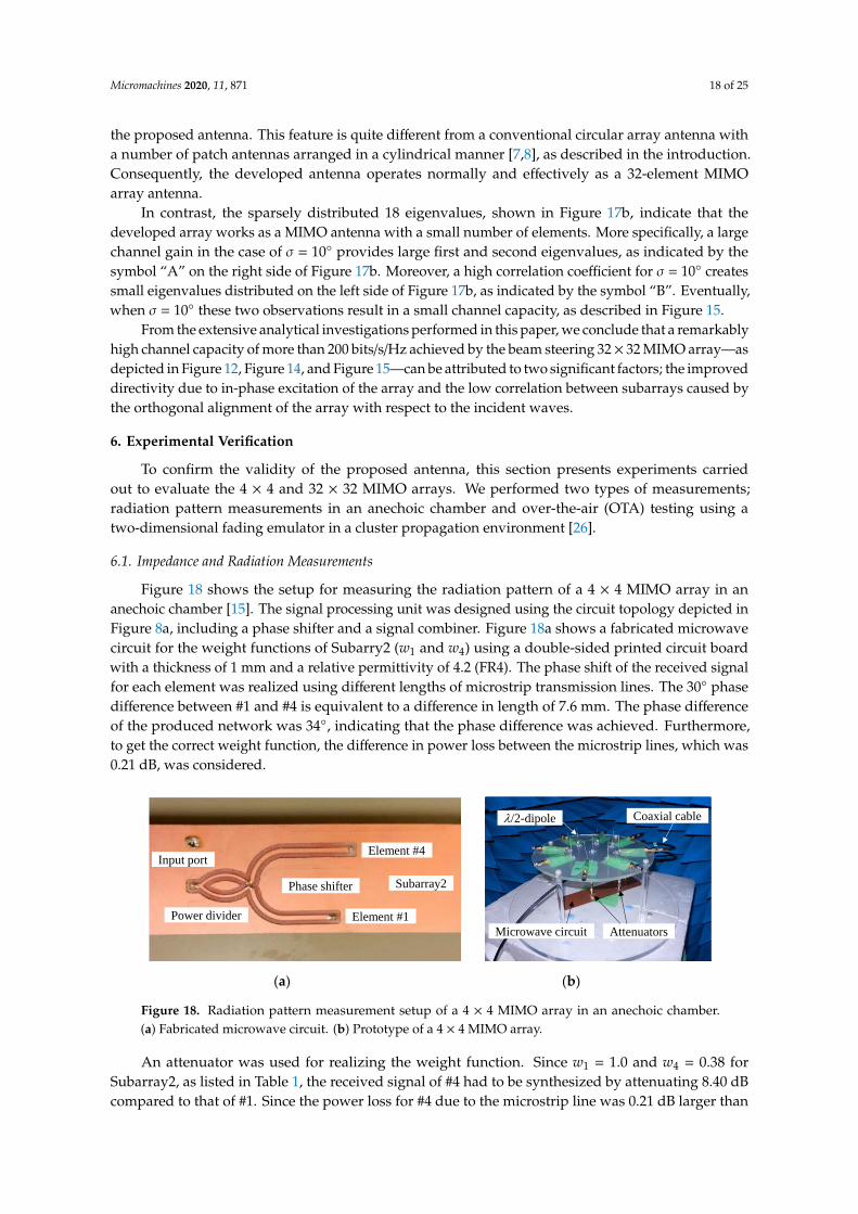
Micromachines 2020, 11, 871 18 of 25
the proposed antenna. This feature is quite different from a conventional circular array antenna witha number of patch antennas arranged in a cylindrical manner [7,8], as described in the introduction.Consequently, the developed antenna operates normally and effectively as a 32-element MIMOarray antenna.
In contrast, the sparsely distributed 18 eigenvalues, shown in Figure 17b, indicate that thedeveloped array works as a MIMO antenna with a small number of elements. More specifically, a largechannel gain in the case of σ = 10◦ provides large first and second eigenvalues, as indicated by thesymbol “A” on the right side of Figure 17b. Moreover, a high correlation coefficient for σ = 10◦ createssmall eigenvalues distributed on the left side of Figure 17b, as indicated by the symbol “B”. Eventually,when σ = 10◦ these two observations result in a small channel capacity, as described in Figure 15.
From the extensive analytical investigations performed in this paper, we conclude that a remarkablyhigh channel capacity of more than 200 bits/s/Hz achieved by the beam steering 32× 32 MIMO array—asdepicted in Figure 12, Figure 14, and Figure 15—can be attributed to two significant factors; the improveddirectivity due to in-phase excitation of the array and the low correlation between subarrays caused bythe orthogonal alignment of the array with respect to the incident waves.
6. Experimental Verification
To confirm the validity of the proposed antenna, this section presents experiments carriedout to evaluate the 4 × 4 and 32 × 32 MIMO arrays. We performed two types of measurements;radiation pattern measurements in an anechoic chamber and over-the-air (OTA) testing using atwo-dimensional fading emulator in a cluster propagation environment [26].
6.1. Impedance and Radiation Measurements
Figure 18 shows the setup for measuring the radiation pattern of a 4 × 4 MIMO array in ananechoic chamber [15]. The signal processing unit was designed using the circuit topology depicted inFigure 8a, including a phase shifter and a signal combiner. Figure 18a shows a fabricated microwavecircuit for the weight functions of Subarry2 (w1 and w4) using a double-sided printed circuit boardwith a thickness of 1 mm and a relative permittivity of 4.2 (FR4). The phase shift of the received signalfor each element was realized using different lengths of microstrip transmission lines. The 30◦ phasedifference between #1 and #4 is equivalent to a difference in length of 7.6 mm. The phase differenceof the produced network was 34◦, indicating that the phase difference was achieved. Furthermore,to get the correct weight function, the difference in power loss between the microstrip lines, which was0.21 dB, was considered.
Micromachines 2020, 11, x 18 of 25
(a) (b)
Figure 17. CDF characteristics of eigenvalues. (a) σ = 60°. (b) σ = 10°.
From the extensive analytical investigations performed in this paper, we conclude that a
remarkably high channel capacity of more than 200 bits/s/Hz achieved by the beam steering 32 × 32
MIMO array—as depicted in Figures 12, 14, and 15—can be attributed to two significant factors; the
improved directivity due to in-phase excitation of the array and the low correlation between
subarrays caused by the orthogonal alignment of the array with respect to the incident waves.
6. Experimental Verification
To confirm the validity of the proposed antenna, this section presents experiments carried out
to evaluate the 4 × 4 and 32 × 32 MIMO arrays. We performed two types of measurements; radiation
pattern measurements in an anechoic chamber and over-the-air (OTA) testing using a two-
dimensional fading emulator in a cluster propagation environment [26].
6.1. Impedance and Radiation Measurements
Figure 18 shows the setup for measuring the radiation pattern of a 4 × 4 MIMO array in an
anechoic chamber [15]. The signal processing unit was designed using the circuit topology depicted
in Figure 8a, including a phase shifter and a signal combiner. Figure 18a shows a fabricated
microwave circuit for the weight functions of Subarry2 (w1 and w4) using a double-sided printed
circuit board with a thickness of 1 mm and a relative permittivity of 4.2 (FR4). The phase shift of the
received signal for each element was realized using different lengths of microstrip transmission lines.
The 30° phase difference between #1 and #4 is equivalent to a difference in length of 7.6 mm. The
phase difference of the produced network was 34°, indicating that the phase difference was achieved.
Furthermore, to get the correct weight function, the difference in power loss between the microstrip
lines, which was 0.21 dB, was considered.
(a) (b)
Figure 18. Radiation pattern measurement setup of a 4 × 4 MIMO array in an anechoic chamber. (a)
Fabricated microwave circuit. (b) Prototype of a 4 × 4 MIMO array.
Eigenvalue
Cum
ula
tive
Per
centa
ge
[%]
100
90
80
70
60
50
40
30
20
10
010-4 10-2 100 102 104
Eigenvalue
Cum
ula
tiv
e P
erce
nta
ge
[%]
100
90
80
70
60
50
40
30
20
10
010-4 10-2 100 102 104
r = 30cm
SNR = 30dB
= 0deg
AB
Input port
Power divider
Phase shifter
Element #4
Element #1
Subarray2
Microwave circuit Attenuators
/2-dipole Coaxial cable
Figure 18. Radiation pattern measurement setup of a 4 × 4 MIMO array in an anechoic chamber.(a) Fabricated microwave circuit. (b) Prototype of a 4 × 4 MIMO array.
An attenuator was used for realizing the weight function. Since w1 = 1.0 and w4 = 0.38 forSubarray2, as listed in Table 1, the received signal of #4 had to be synthesized by attenuating 8.40 dBcompared to that of #1. Since the power loss for #4 due to the microstrip line was 0.21 dB larger than
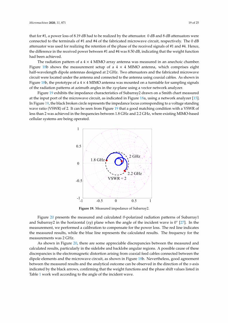
Micromachines 2020, 11, 871 19 of 25
that for #1, a power loss of 8.19 dB had to be realized by the attenuator. 0 dB and 8 dB attenuators wereconnected to the terminals of #1 and #4 of the fabricated microwave circuit, respectively. The 0 dBattenuator was used for realizing the retention of the phase of the received signals of #1 and #4. Hence,the difference in the received power between #1 and #4 was 8.50 dB, indicating that the weight functionhad been achieved.
The radiation pattern of a 4 × 4 MIMO array antenna was measured in an anechoic chamber.Figure 18b shows the measurement setup of a 4 × 4 MIMO antenna, which comprises eighthalf-wavelength dipole antennas designed at 2 GHz. Two attenuators and the fabricated microwavecircuit were located under the antenna and connected to the antenna using coaxial cables. As shown inFigure 18b, the prototype of a 4 × 4 MIMO antenna was mounted on a turntable for sampling signalsof the radiation patterns at azimuth angles in the xy-plane using a vector network analyzer.
Figure 19 exhibits the impedance characteristics of Subarray2 drawn on a Smith chart measuredat the input port of the microwave circuit, as indicated in Figure 18a, using a network analyzer [15].In Figure 19, the black broken circle represents the impedance locus corresponding to a voltage standingwave ratio (VSWR) of 2. It can be seen from Figure 19 that a good matching condition with a VSWR ofless than 2 was achieved in the frequencies between 1.8 GHz and 2.2 GHz, where existing MIMO-basedcellular systems are being operated.
Micromachines 2020, 11, x 19 of 25
An attenuator was used for realizing the weight function. Since w1 = 1.0 and w4 = 0.38 for Subarray2, as listed in Table 1, the received signal of #4 had to be synthesized by attenuating 8.40 dB compared to that of #1. Since the power loss for #4 due to the microstrip line was 0.21 dB larger than that for #1, a power loss of 8.19 dB had to be realized by the attenuator. 0 dB and 8 dB attenuators were connected to the terminals of #1 and #4 of the fabricated microwave circuit, respectively. The 0 dB attenuator was used for realizing the retention of the phase of the received signals of #1 and #4. Hence, the difference in the received power between #1 and #4 was 8.50 dB, indicating that the weight function had been achieved.
The radiation pattern of a 4 × 4 MIMO array antenna was measured in an anechoic chamber. Figure 18b shows the measurement setup of a 4 × 4 MIMO antenna, which comprises eight half-wavelength dipole antennas designed at 2 GHz. Two attenuators and the fabricated microwave circuit were located under the antenna and connected to the antenna using coaxial cables. As shown in Figure 18b, the prototype of a 4 × 4 MIMO antenna was mounted on a turntable for sampling signals of the radiation patterns at azimuth angles in the xy-plane using a vector network analyzer.
Figure 19 exhibits the impedance characteristics of Subarray2 drawn on a Smith chart measured at the input port of the microwave circuit, as indicated in Figure 18a, using a network analyzer [15]. In Figure 19, the black broken circle represents the impedance locus corresponding to a voltage standing wave ratio (VSWR) of 2. It can be seen from Figure 19 that a good matching condition with a VSWR of less than 2 was achieved in the frequencies between 1.8 GHz and 2.2 GHz, where existing MIMO-based cellular systems are being operated.
Figure 19. Measured impedance of Subarray2.
Figure 20 presents the measured and calculated θ-polarized radiation patterns of Subarray1 and Subarray2 in the horizontal (xy) plane when the angle of the incident wave is 0° [27]. In the measurement, we performed a calibration to compensate for the power loss. The red line indicates the measured results, while the blue line represents the calculated results. The frequency for the measurements was 2 GHz.
As shown in Figure 20, there are some appreciable discrepancies between the measured and calculated results, particularly in the sidelobe and backlobe angular regions. A possible cause of these discrepancies is the electromagnetic distortion arising from coaxial feed cables connected between the dipole elements and the microwave circuit, as shown in Figure 18b. Nevertheless, good agreement between the measured results and the analytical outcome can be observed in the direction of the x-axis indicated by the black arrows, confirming that the weight functions and the phase shift values listed in Table 1 work well according to the angle of the incident wave.
-1 -0.5 0 0.5 1 -1
-0.5
0
0.5
1
2.2 GHz
1.8 GHz2 GHz
VSWR = 2
Figure 19. Measured impedance of Subarray2.
Figure 20 presents the measured and calculated θ-polarized radiation patterns of Subarray1and Subarray2 in the horizontal (xy) plane when the angle of the incident wave is 0◦ [27]. In themeasurement, we performed a calibration to compensate for the power loss. The red line indicatesthe measured results, while the blue line represents the calculated results. The frequency for themeasurements was 2 GHz.
As shown in Figure 20, there are some appreciable discrepancies between the measured andcalculated results, particularly in the sidelobe and backlobe angular regions. A possible cause of thesediscrepancies is the electromagnetic distortion arising from coaxial feed cables connected between thedipole elements and the microwave circuit, as shown in Figure 18b. Nevertheless, good agreementbetween the measured results and the analytical outcome can be observed in the direction of the x-axisindicated by the black arrows, confirming that the weight functions and the phase shift values listed inTable 1 work well according to the angle of the incident wave.
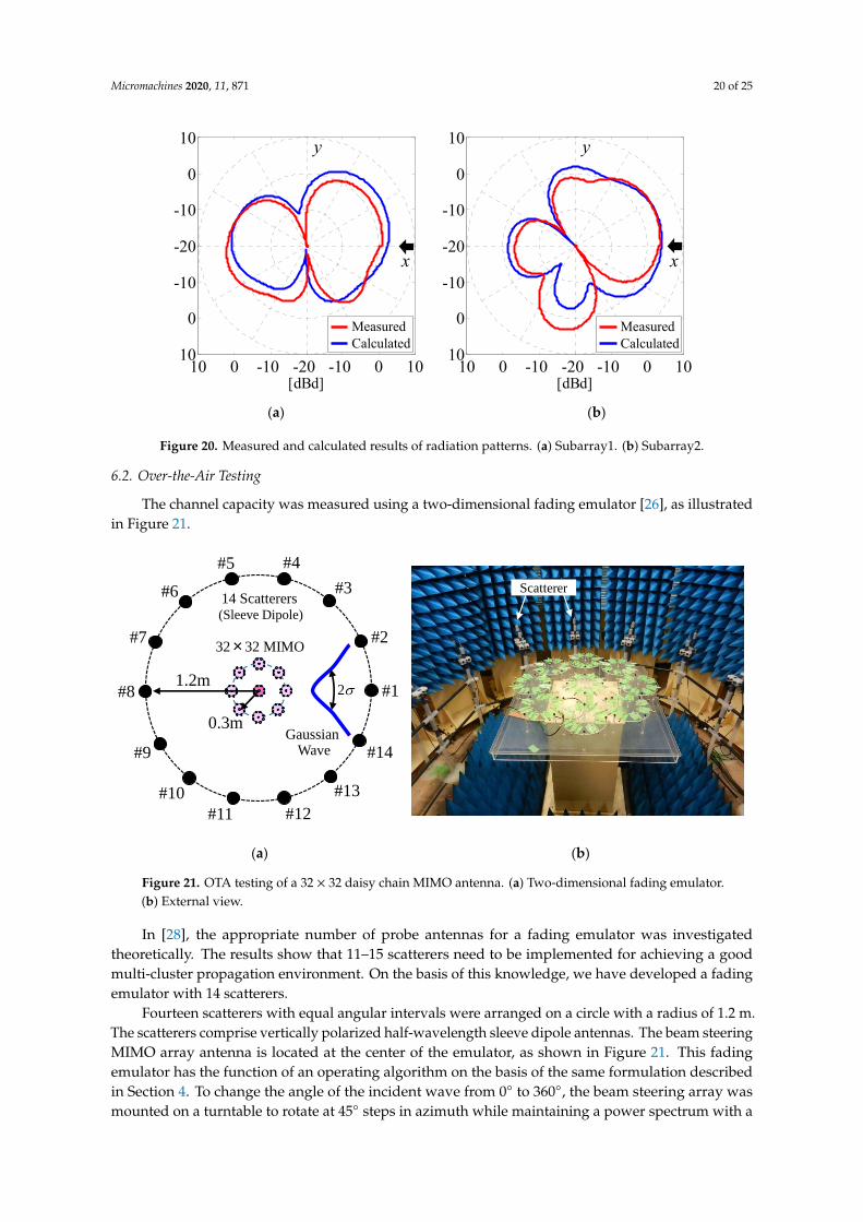
Micromachines 2020, 11, 871 20 of 25Micromachines 2020, 11, x 20 of 25
(a) (b)
Figure 20. Measured and calculated results of radiation patterns. (a) Subarray1. (b) Subarray2.
6.2. Over-the-Air Testing
The channel capacity was measured using a two-dimensional fading emulator [26], as illustrated in Figure 21.
(a) (b)
Figure 21. OTA testing of a 32 × 32 daisy chain MIMO antenna. (a) Two-dimensional fading emulator. (b) External view.
In [28], the appropriate number of probe antennas for a fading emulator was investigated theoretically. The results show that 11–15 scatterers need to be implemented for achieving a good multi-cluster propagation environment. On the basis of this knowledge, we have developed a fading emulator with 14 scatterers.
Fourteen scatterers with equal angular intervals were arranged on a circle with a radius of 1.2 m. The scatterers comprise vertically polarized half-wavelength sleeve dipole antennas. The beam steering MIMO array antenna is located at the center of the emulator, as shown in Figure 21. This fading emulator has the function of an operating algorithm on the basis of the same formulation described in Section 4. To change the angle of the incident wave from 0° to 360°, the beam steering array was mounted on a turntable to rotate at 45° steps in azimuth while maintaining a power
10 0 -10 -20 -10 0 1010
0
-10
-20
-10
0
10
[dBd]
10 0 -10 -20 -10 0 1010
0
-10
-20
-10
0
10
[dBd]
x
y
x
y
MeasuredCalculated
MeasuredCalculated
Figure 20. Measured and calculated results of radiation patterns. (a) Subarray1. (b) Subarray2.
6.2. Over-the-Air Testing
The channel capacity was measured using a two-dimensional fading emulator [26], as illustratedin Figure 21.
Micromachines 2020, 11, x 20 of 25
(a) (b)
Figure 20. Measured and calculated results of radiation patterns. (a) Subarray1. (b) Subarray2.
6.2. Over-the-Air Testing
The channel capacity was measured using a two-dimensional fading emulator [26], as illustrated
in Figure 21.
(a) (b)
Figure 21. OTA testing of a 32 × 32 daisy chain MIMO antenna. (a) Two-dimensional fading emulator.
(b) External view.
In [28], the appropriate number of probe antennas for a fading emulator was investigated
theoretically. The results show that 11–15 scatterers need to be implemented for achieving a good
multi-cluster propagation environment. On the basis of this knowledge, we have developed a fading
emulator with 14 scatterers.
Fourteen scatterers with equal angular intervals were arranged on a circle with a radius of 1.2
m. The scatterers comprise vertically polarized half-wavelength sleeve dipole antennas. The beam
steering MIMO array antenna is located at the center of the emulator, as shown in Figure 21. This
fading emulator has the function of an operating algorithm on the basis of the same formulation
described in Section 4. To change the angle of the incident wave from 0° to 360°, the beam steering
array was mounted on a turntable to rotate at 45° steps in azimuth while maintaining a power
10 0 -10 -20 -10 0 1010
0
-10
-20
-10
0
10
[dBd]
10 0 -10 -20 -10 0 1010
0
-10
-20
-10
0
10
[dBd]
x
y
x
y
Measured
Calculated
Measured
Calculated
Scatterer
(Sleeve Dipole)
14 Scatterers
1.2m
0.3m
32×32 MIMO
#1
#2
#3
#4#5
#6
#7
#8
#9
#10
#11 #12
#13
#14Gaussian
Wave
2
Figure 21. OTA testing of a 32 × 32 daisy chain MIMO antenna. (a) Two-dimensional fading emulator.(b) External view.
In [28], the appropriate number of probe antennas for a fading emulator was investigatedtheoretically. The results show that 11–15 scatterers need to be implemented for achieving a goodmulti-cluster propagation environment. On the basis of this knowledge, we have developed a fadingemulator with 14 scatterers.
Fourteen scatterers with equal angular intervals were arranged on a circle with a radius of 1.2 m.The scatterers comprise vertically polarized half-wavelength sleeve dipole antennas. The beam steeringMIMO array antenna is located at the center of the emulator, as shown in Figure 21. This fadingemulator has the function of an operating algorithm on the basis of the same formulation describedin Section 4. To change the angle of the incident wave from 0◦ to 360◦, the beam steering array wasmounted on a turntable to rotate at 45◦ steps in azimuth while maintaining a power spectrum with a
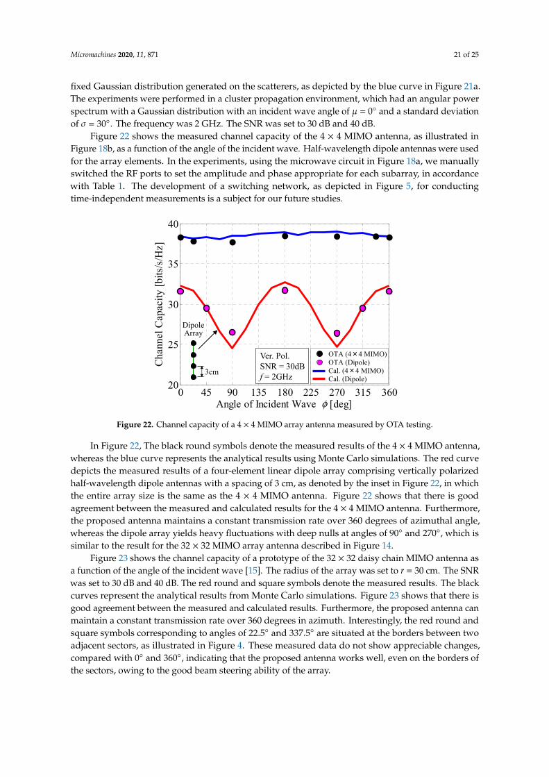
Micromachines 2020, 11, 871 21 of 25
fixed Gaussian distribution generated on the scatterers, as depicted by the blue curve in Figure 21a.The experiments were performed in a cluster propagation environment, which had an angular powerspectrum with a Gaussian distribution with an incident wave angle of µ = 0◦ and a standard deviationof σ = 30◦. The frequency was 2 GHz. The SNR was set to 30 dB and 40 dB.
Figure 22 shows the measured channel capacity of the 4 × 4 MIMO antenna, as illustrated inFigure 18b, as a function of the angle of the incident wave. Half-wavelength dipole antennas were usedfor the array elements. In the experiments, using the microwave circuit in Figure 18a, we manuallyswitched the RF ports to set the amplitude and phase appropriate for each subarray, in accordancewith Table 1. The development of a switching network, as depicted in Figure 5, for conductingtime-independent measurements is a subject for our future studies.
Micromachines 2020, 11, x 21 of 25
spectrum with a fixed Gaussian distribution generated on the scatterers, as depicted by the blue curve in Figure 21a. The experiments were performed in a cluster propagation environment, which had an angular power spectrum with a Gaussian distribution with an incident wave angle of µ = 0° and a standard deviation of σ = 30°. The frequency was 2 GHz. The SNR was set to 30 dB and 40 dB.
Figure 22 shows the measured channel capacity of the 4 × 4 MIMO antenna, as illustrated in Figure 18b, as a function of the angle of the incident wave. Half-wavelength dipole antennas were used for the array elements. In the experiments, using the microwave circuit in Figure 18a, we manually switched the RF ports to set the amplitude and phase appropriate for each subarray, in accordance with Table 1. The development of a switching network, as depicted in Figure 5, for conducting time-independent measurements is a subject for our future studies.
Figure 22. Channel capacity of a 4 × 4 MIMO array antenna measured by OTA testing.
In Figure 22, The black round symbols denote the measured results of the 4 × 4 MIMO antenna, whereas the blue curve represents the analytical results using Monte Carlo simulations. The red curve depicts the measured results of a four-element linear dipole array comprising vertically polarized half-wavelength dipole antennas with a spacing of 3 cm, as denoted by the inset in Figure 22, in which the entire array size is the same as the 4 × 4 MIMO antenna. Figure 22 shows that there is good agreement between the measured and calculated results for the 4 × 4 MIMO antenna. Furthermore, the proposed antenna maintains a constant transmission rate over 360 degrees of azimuthal angle, whereas the dipole array yields heavy fluctuations with deep nulls at angles of 90° and 270°, which is similar to the result for the 32 × 32 MIMO array antenna described in Figure 14.
Figure 23 shows the channel capacity of a prototype of the 32 × 32 daisy chain MIMO antenna as a function of the angle of the incident wave [15]. The radius of the array was set to r = 30 cm. The SNR was set to 30 dB and 40 dB. The red round and square symbols denote the measured results. The black curves represent the analytical results from Monte Carlo simulations. Figure 23 shows that there is good agreement between the measured and calculated results. Furthermore, the proposed antenna can maintain a constant transmission rate over 360 degrees in azimuth. Interestingly, the red round and square symbols corresponding to angles of 22.5° and 337.5° are situated at the borders between two adjacent sectors, as illustrated in Figure 4. These measured data do not show appreciable changes, compared with 0° and 360°, indicating that the proposed antenna works well, even on the borders of the sectors, owing to the good beam steering ability of the array.
0 45 90 135 180 225 270 315 36020
25
30
35
40
Angle of Incident Wave φ [deg]
Cha
nnel
Cap
acity
[bits
/s/H
z]
OTA (4×4 MIMO)OTA (Dipole)Cal. (4×4 MIMO)Cal. (Dipole)
Ver. Pol.SNR = 30dBf = 2GHz
DipoleArray
3cm
Figure 22. Channel capacity of a 4 × 4 MIMO array antenna measured by OTA testing.
In Figure 22, The black round symbols denote the measured results of the 4 × 4 MIMO antenna,whereas the blue curve represents the analytical results using Monte Carlo simulations. The red curvedepicts the measured results of a four-element linear dipole array comprising vertically polarizedhalf-wavelength dipole antennas with a spacing of 3 cm, as denoted by the inset in Figure 22, in whichthe entire array size is the same as the 4 × 4 MIMO antenna. Figure 22 shows that there is goodagreement between the measured and calculated results for the 4 × 4 MIMO antenna. Furthermore,the proposed antenna maintains a constant transmission rate over 360 degrees of azimuthal angle,whereas the dipole array yields heavy fluctuations with deep nulls at angles of 90◦ and 270◦, which issimilar to the result for the 32 × 32 MIMO array antenna described in Figure 14.
Figure 23 shows the channel capacity of a prototype of the 32 × 32 daisy chain MIMO antenna asa function of the angle of the incident wave [15]. The radius of the array was set to r = 30 cm. The SNRwas set to 30 dB and 40 dB. The red round and square symbols denote the measured results. The blackcurves represent the analytical results from Monte Carlo simulations. Figure 23 shows that there isgood agreement between the measured and calculated results. Furthermore, the proposed antenna canmaintain a constant transmission rate over 360 degrees in azimuth. Interestingly, the red round andsquare symbols corresponding to angles of 22.5◦ and 337.5◦ are situated at the borders between twoadjacent sectors, as illustrated in Figure 4. These measured data do not show appreciable changes,compared with 0◦ and 360◦, indicating that the proposed antenna works well, even on the borders ofthe sectors, owing to the good beam steering ability of the array.

Micromachines 2020, 11, 871 22 of 25Micromachines 2020, 11, x 22 of 25
Figure 23. Channel capacity of a 32 × 32 MIMO array antenna measured by OTA testing.
In Section 5.3, the channel gain and correlation were obtained from a theoretical investigation using Monte Carlo simulation, as shown in Figure 16. In this section, to investigate the mechanism for achieving a large channel capacity in an empirical way, we took an experimental approach by means of OTA testing to evaluate the channel gain and correlation.
Figure 24 shows the channel gain and correlation coefficient of each subarray of the 32 × 32 MIMO array as a function of the number of the subarray [15]. The black curves indicate the analytical results using Monte Carlo simulation, while the red curves indicate the measured results through OTA testing, depicted in Figure 21. The blue and red subarrays, indicated by the inset in Figure 24a, represent that these subarrays. Subarrays 1–4 and Subarrays 17–20 are located in the forward and backward directions with respect to the incident wave. The blue and red arrows included in the upper part of Figure 24a indicate the locations of Subarrays 1–4 and Subarrays 17–20 on the lateral axis.
(a) (b)
Figure 24. Channel gain and correlation of a 32 × 32 MIMO array measured by OTA testing. (a) Channel gain. (b) Correlation.
Figure 24a shows that Subarrays 1–4, which face the incident wave, provide a large channel gain of more than 2.15 dB, meaning that these subarrays operate more effectively than a conventional dipole antenna. On the other hand, for Subarrays 17–20, the channel gain is significantly reduced to
0 45 90 135 180 225 270 315 3600
50
100
150
200
250
300
350
400
Angle of Incident Wave φ [deg]
Chan
nel C
apac
ity [b
its/s/
Hz]
Cal. (SNR = 40dB)OTA (SNR = 40dB)Cal. (SNR = 30dB)OTA (SNR = 30dB)
r = 30cmσ = 30degf = 2GHz
1 2 3 4 5 6 7 8 9 10 11 12 13 14 15 16 17 18 19 20 21 22 23 24 25 26 27 28 29 30 31 32 1 2 3 4 5 6 7 8 9 1011121314 15161718 1920212223 24252627 28293031 32
Abs
olut
e of
Com
plex
Cor
rela
tion
10.90.80.70.60.50.40.30.20.1
0
Number of Subarray
r = 30cmSNR = 30dBφ = 0degσ = 30deg
Aver
age
of C
hann
el G
ain
[dB]
Number of Subarray
109876543210
-1-2-3-4-5-6
r = 30cmSNR = 30dBφ = 0degσ = 30deg
1-4
5-89-12
13-16
17-20
21-2425-28
29-32
2σ
IncidentWave
Subarrays 1-4
Subarrays 17-20
OTA TestingMonte Carlo
OTA TestingMonte Carlo
Figure 23. Channel capacity of a 32 × 32 MIMO array antenna measured by OTA testing.
In Section 5.3, the channel gain and correlation were obtained from a theoretical investigationusing Monte Carlo simulation, as shown in Figure 16. In this section, to investigate the mechanism forachieving a large channel capacity in an empirical way, we took an experimental approach by means ofOTA testing to evaluate the channel gain and correlation.
Figure 24 shows the channel gain and correlation coefficient of each subarray of the 32 × 32 MIMOarray as a function of the number of the subarray [15]. The black curves indicate the analytical resultsusing Monte Carlo simulation, while the red curves indicate the measured results through OTA testing,depicted in Figure 21. The blue and red subarrays, indicated by the inset in Figure 24a, represent thatthese subarrays. Subarrays 1–4 and Subarrays 17–20 are located in the forward and backward directionswith respect to the incident wave. The blue and red arrows included in the upper part of Figure 24aindicate the locations of Subarrays 1–4 and Subarrays 17–20 on the lateral axis.
Micromachines 2020, 11, x 22 of 25
Figure 23. Channel capacity of a 32 × 32 MIMO array antenna measured by OTA testing.
In Section 5.3, the channel gain and correlation were obtained from a theoretical investigation
using Monte Carlo simulation, as shown in Figure 16. In this section, to investigate the mechanism
for achieving a large channel capacity in an empirical way, we took an experimental approach by
means of OTA testing to evaluate the channel gain and correlation.
Figure 24 shows the channel gain and correlation coefficient of each subarray of the 32 × 32
MIMO array as a function of the number of the subarray [15]. The black curves indicate the analytical
results using Monte Carlo simulation, while the red curves indicate the measured results through
OTA testing, depicted in Figure 21. The blue and red subarrays, indicated by the inset in Figure 24a,
represent that these subarrays. Subarrays 1–4 and Subarrays 17–20 are located in the forward and
backward directions with respect to the incident wave. The blue and red arrows included in the upper
part of Figure 24a indicate the locations of Subarrays 1–4 and Subarrays 17–20 on the lateral axis.
(a) (b)
Figure 24. Channel gain and correlation of a 32 × 32 MIMO array measured by OTA testing. (a)
Channel gain. (b) Correlation.
Figure 24a shows that Subarrays 1–4, which face the incident wave, provide a large channel gain
of more than 2.15 dB, meaning that these subarrays operate more effectively than a conventional
dipole antenna. On the other hand, for Subarrays 17–20, the channel gain is significantly reduced to
0 45 90 135 180 225 270 315 3600
50
100
150
200
250
300
350
400
Angle of Incident Wave [deg]
Ch
ann
el C
apac
ity
[b
its/
s/H
z]
Cal. (SNR = 40dB)
OTA (SNR = 40dB)
Cal. (SNR = 30dB)
OTA (SNR = 30dB)
r = 30cm
= 30deg
f = 2GHz
1 2 3 4 5 6 7 8 9 10 11 12 13 14 15 16 17 18 19 20 21 22 23 24 25 26 27 28 29 30 31 32 1 2 3 4 5 6 7 8 9 1011121314 15161718 1920212223 24252627 28293031 32
Ab
solu
te o
f C
om
ple
x C
orr
elat
ion
1
0.9
0.8
0.7
0.6
0.5
0.4
0.3
0.2
0.1
0
Number of Subarray
r = 30cm
SNR = 30dB
= 0deg
= 30deg
Av
erag
e o
f C
han
nel
Gai
n [
dB
]
Number of Subarray
109876543210
-1-2-3-4-5-6
r = 30cm
SNR = 30dB
= 0deg
= 30deg
1-4
5-8
9-12
13-16
17-20
21-2425-28
29-32
2
Incident
Wave
Subarrays 1-4
Subarrays 17-20
OTA Testing
Monte Carlo
OTA Testing
Monte Carlo
Figure 24. Channel gain and correlation of a 32 × 32 MIMO array measured by OTA testing. (a) Channelgain. (b) Correlation.
Figure 24a shows that Subarrays 1–4, which face the incident wave, provide a large channel gainof more than 2.15 dB, meaning that these subarrays operate more effectively than a conventional dipoleantenna. On the other hand, for Subarrays 17–20, the channel gain is significantly reduced to less than

Micromachines 2020, 11, 871 23 of 25
0 dB. This implies that these subarrays do not contribute to the formation of subchannels available forMIMO transmission. It is worth noting that, in Figure 24a, there is an appreciable discrepancy betweenthe OTA measurements and the analytical outcomes. This is due to the fact that Subarrays 1–4, 5–8,and 29–32, located in the forward direction with respect to the incident wave, receive strong signalsfrom the scatterers because of the small distance between these subarrays and the scatterers emittinga cluster wave, as shown in Figure 21a. In contrast, Subarrays 13–16, 17–20, and 21–24, located atthe back with respect to the direction of the incident wave, receive weak signals because of the largedistance between these subarrays and the scatterers.
Figure 24b shows that, in the OTA measurements, the correlation coefficient increases in a periodicmanner, which is not observed in the analytical outcome from the Monte Carlo simulations. A possiblecause of this phenomenon is the insufficient orthogonality between the incident waves coming from thescatterers, because, in the current experiment, the number of scatterers in the emulator is 14, which isconsiderably smaller than the number of subarrays, i.e., 32. Nevertheless, it can be seen from Figure 24bthat except for the correlation between those particular subarray numbers showing a periodic increase,the correlation coefficients are less than 0.5 over the entire array because of the orthogonal alignmentbetween the MIMO array and the incident waves.
7. Conclusions
This paper presents a 32 × 32 MIMO antenna system with the ability to perform full-azimuthbeam steering. Analyses revealed that the proposed antenna system can provide a maximum channelcapacity of 277 bits/s/Hz at an SNR of 30 dB when the radius of the array is 30 cm, which is equivalentto 27.7 Gbps with a bandwidth of 100 MHz. It was clarified that this remarkably high channel capacityis due to two significant factors; the improved directivity due to the optimum in-phase excitationand the low correlation between the subarrays due to the orthogonal alignment of the array withrespect to the incident waves. We further performed an experimental validation of the channel capacityusing over-the-air (OTA) testing. The results show that the proposed antenna can maintain a constantchannel capacity over 360 degrees in azimuth.
The developed technology can be applied to the achievement of a 64 × 64 MIMO array [29] anda 128 × 128 MIMO array [18] in pursuit of much larger transmission rates in the 5 GHz frequencyband. Thereby, the daisy chain array structure proposed in this paper provides a strong solution forrealizing a much higher order MIMO array antenna at higher frequencies, such as in the 5.9 GHz band,where the emerging vehicle-to-everything (V2X) and cellular-V2X (C-V2X) technologies are anticipatedto be operated for future connected cars [30–32].
Author Contributions: Conceptualization, K.O.; Funding acquisition, K.H.; Investigation, K.H.; Methodology,K.H.; Validation, T.F.; Writing—original draft, K.H. All authors provided critical feedback and helped shape theresearch, analysis, and manuscript. All authors have read and agreed to the published version of the manuscript.
Funding: This research and development work was supported by the MIC/SCOPE #205005002.
Acknowledgments: The authors acknowledge the funding from the MIC/SCOPE #205005002.
Conflicts of Interest: The authors declare no conflict of interest.
References
1. Rusek, F.; Persson, D.; Lau, B.K.; Larsson, E.G.; Marzetta, T.L.; Edfors, O.; Tufvesson, F. Scaling Up MIMO:Opportunities and challenges with very large MIMO. IEEE Signal. Process. Mag. 2012, 30, 40–60. [CrossRef]
2. Larsson, E.G.; Edfors, O.; Tufvesson, F.; Marzetta, T.L. Massive MIMO for Next Generation Wireless Systems.IEEE Commun. Mag. 2014, 52, 186–195. [CrossRef]
3. Kibaroglu, K.; Sayginer, M.; Phelps, T.; Rebeiz, G.M. A 64-Element 28-GHz Phased-Array TransceiverWith 52-dBm EIRP and 8–12-Gb/s 5G Link at 300 Meters without Any Calibration. IEEE Trans. Microw.Theory Technol. 2018, 66, 5796–5811. [CrossRef]

Micromachines 2020, 11, 871 24 of 25
4. Yamaguchi, S.; Nakamizo, H.; Shinjo, S.; Tsutsumi, K.; Fukasawa, T.; Miyashita, H. Development of activephased array antenna for high SHF wideband massive MIMO in 5G. In Proceedings of the 2017 IEEEInternational Symposium on Antennas and Propagation & USNC/URSI National Radio Science Meeting,San Diego, CA, USA, 9–14 July 2017; pp. 1463–1464.
5. Mao, C.-X.; Gao, S.; Wang, Y. Broadband High-Gain Beam-Scanning Antenna Array for Millimeter-WaveApplications. IEEE Trans. Antennas Propag. 2017, 65, 4864–4868. [CrossRef]
6. Al-Tarifi, M.A.; Faouri, Y.S.; Sharawi, M.S. A printed 16 ports massive MIMO antenna system with directiveport beams. In Proceedings of the 2016 IEEE 5th Asia-Pacific Conference on Antennas and Propagation(APCAP), Kaohsiung, Taiwan, 26–29 July 2016; pp. 125–126.
7. Kataoka, R.; Nishimori, K.; Tran, N.; Imai, T.; Makino, H. Interference Reduction Characteristics by CircularArray Based Massive MIMO in a Real Microcell Environment. IEICE Trans. Commun. 2015, 1447–1455.[CrossRef]
8. Schneider, C.; Thoma, R.S. Empirical Study of Higher Order MIMO Capacity at 2.53 GHz in Urban Macro Cell.In Proceedings of the 2013 7th European Conference on Antennas and Propagation (EuCAP), Gothenburg,Sweden, 8–12 April 2013; pp. 477–481.
9. Mumtaz, S.; Huq, K.; Ashraf, M.; Rodriguez, J.; Monterio, V.; Politisand, C. Cognitive VehicularCommunication for 5G. IEEE Commun. Mag. 2015, 53, 109–117. [CrossRef]
10. Chong, C.; Watanabe, F.; Kitao, K.; Imai, T.; Inamura, H. Evolution Trends of Wireless MIMO ChannelModeling towards IMT-Advanced. IEICE Trans. Commun. 2009, 2773–2788. [CrossRef]
11. Kuchar, A.; Rossi, J.; Bonek, E. Directional macro-cell channel characterization from urban measurements.IEEE Trans. Antennas Propag. 2000, 48, 137–146. [CrossRef]
12. Honda, K.; Fukushima, T.; Ogawa, K. Dual-Circular 8 × 8 MIMO Array with Synchronized Beam Scan forOver-Gbps Inter-Vehicle Communications. In Proceedings of the Progress in Electromagnetics ResearchSymposium 2018 (PIERS2018), Toyama, Japan, 1–4 August 2018; pp. 1989–1994.
13. Fukushima, T.; Honda, K.; Ogawa, K. 140 bps/Hz 16 × 16 MIMO Whole Azimuth Beam Steering Arrayfor Connected Car Applications. In Proceedings of the 2018 Asia-Pacific Microwave Conference (APMC),Kyoto, Japan, 6–9 November 2018; pp. 503–505.
14. Narukawa, N.; Fukushima, T.; Honda, K.; Ogawa, K. Daisy Chain MIMO Antenna for Whole AzimuthTens-of-Gigabit Connected Cars. In Proceedings of the 2019 URSI International Symposium on ElectromagneticTheory (EMTS), San Diego, CA, USA, 27–31 May 2019; pp. 1–4.
15. Fukushima, T.; Narukawa, N.; Honda, K.; Ogawa, K. Over-the-Air Testing of a 32 × 32 Daisy Chain MIMOAntenna. In Proceedings of the Progress in Electromagnetics Research Symposium 2019 (PIERS2019),Roma, Italy, 17–20 June 2019; pp. 824–830.
16. Honda, K.; Iwamoto, D.; Ogawa, K. Angle of Arrival Estimation Embedded in a Circular Phased Array4 × 4 MIMO Antenna. In Proceedings of the 2017 IEEE Asia Pacific Microwave Conference (APMC),Kuala Lumpur, Malaysia, 13–16 November 2017; pp. 93–96.
17. Iwamoto, D.; Narukawa, N.; Honda, K.; Ogawa, K. Experiments on Interferometric Angle of ArrivalEstimation Using a Simple Weight Network. In Proceedings of the 2018 International Symposium onAntennas and Propagation (ISAP), Busan, Korea, 23–26 October 2018; pp. 351–352.
18. Narukawa, N.; Fukushima, T.; Honda, K.; Ogawa, K. Daisy Chain MIMO Antenna: A Big Challenge toFull-Azimuth 100 Gbps Capacity. In Proceedings of the Progress in Electromagnetics Research Symposium2019 (PIERS2019), Roma, Italy, 17–20 June 2019; pp. 817–823.
19. Honda, K.; Fukushima, T.; Ogawa, K. Development of a Circular Phased Array 4 × 4 MIMO Antenna forAd-hoc Connected Car System. In Proceedings of the 2017 IEEE Asia Pacific Microwave Conference (APMC),Kuala Lumpur, Malaysia, 13–16 November 2017; pp. 795–798.
20. Buehrer, R.M. The impact of angular energy distribution on spatial correlation. In Proceedings of the IEEE56th Vehicular Technology Conference, Vancouver, BC, Canada, 24–28 September 2002; pp. 1173–1177.
21. 3GPP-3GPP2 Spatial Channel Model Ad-hoc Group. Spatial Channel, Model for MIMO Systems. 3GPP and3GPP2 Technical Report. 2003. Available online: http://www.3gpp.org (accessed on 1 August 2020).
22. Ogawa, K.; Yamamoto, A.; Takada, J. Multipath Performance of Handset Adaptive Array Antennas in theVicinity of a Human Operator. IEEE Trans. Antennas Propag. 2005, 53, 2422–2436. [CrossRef]

Micromachines 2020, 11, 871 25 of 25
23. Ogawa, K.; Iwai, H.; Yamamoto, A.; Takada, J. Channel Capacity of a Handset MIMO Antenna Influenced bythe Effects of 3D Angular Spectrum, Polarization, and Operator. In Proceedings of the 2006 IEEE Antennasand Propagation Society International Symposium, Albuquerque, NM, USA, 9–14 July 2006; pp. 153–156.
24. Chuah, C.-N.; Kahn, J.M.; Tse, D.N.C. Capacity Scaling in MIMO Wireless Systems under Correlated Fading.IEEE Trans. Inf. Theory 2002, 48, 637–650. [CrossRef]
25. Taga, T. Analysis for mean effective gain of mobile antennas in land mobile radio environments. IEEE Trans.Veh. Technol. 1990, 39, 117–131. [CrossRef]
26. Sakata, T.; Yamamoto, A.; Ogawa, K.; Iwai, H.; Takada, J.; Sakaguchi, K. A Spatial Fading Emulator forEvaluation of MIMO Antennas in a Cluster Environment. IEICE Trans. Commun. 2014, 2127–2135. [CrossRef]
27. Fukushima, T.; Honda, K.; Ogawa, K. Directivity Measurement of Circular Phased Array 4 × 4 MIMOAntenna. In Proceedings of the Progress in Electromagnetics Research Symposium 2018 (PIERS2018),Toyama, Japan, 1–4 August 2018; pp. 1984–1988.
28. Imai, T.; Okano, Y.; Koshino, K.; Saito, K.; Miura, S. Theoretical Analysis of Adequate Number ofProbe Antennas in Spatial Channel Emulator for MIMO Performance Evaluation of Mobile Terminals.In Proceedings of the Fourth European Conference on Antennas and Propagation (EuCAP), Barcelona, Spain,12–16 April 2010; pp. 1–5.
29. Narukawa, N.; Fukushima, T.; Honda, K.; Ogawa, K. 64× 64 MIMO Antenna Arranged in a Daisy Chain ArrayStructure at 50 Gbps Capacity. In Proceedings of the 2019 URSI International Symposium on ElectromagneticTheory (EMTS), San Diego, CA, USA, 27–31 May 2019; pp. 1–4.
30. 3G Partnership Project. Study on LTE-Based V2X Services; TR 36.885 v14.0.0; 3GPP: Sophia Antipolis,France, 2016.
31. Chen, S.; Hu, J.; Shi, Y.; Zhao, L. LTE-V: A TD-LTE-Based V2X Solution for Future Vehicular Network.IEEE Internet Things J. 2016, 3, 997–1005. [CrossRef]
32. MacHardy, Z.; Khan, A.; Obana, K.; Iwashina, S. V2X Access Technologies: Regulation, Research,and Remaining Challenges. IEEE Commun. Surv. Tutor. 2018, 20, 1858–1877. [CrossRef]
© 2020 by the authors. Licensee MDPI, Basel, Switzerland. This article is an open accessarticle distributed under the terms and conditions of the Creative Commons Attribution(CC BY) license (http://creativecommons.org/licenses/by/4.0/).