Functional Mockup Interface 2.0: The Standard for Tool independent

Functional Mockup Interface 2.0: The Standard for Tool independent Exchange of Simulation Models

T. Blochwitz1, M. Otter2,

J. Akesson3, M. Arnold4, C. Clauß5, H. Elmqvist6 M. Friedrich7, A. Junghanns8, J. Mauss8, D. Neumerkel9, H. Olsson6,, A. Viel10

Germany: 1ITI GmbH, Dresden; 2DLR Oberpfaffenhofen; 4University of Halle, 5Fraunhofer IIS EAS, Dresden; 7SIMPACK, Gilching; 8QTronic, Berlin;9Daimler AG, Stuttgart;

Sweden: 6Dassault Systèmes, Lund; 3Modelon, Lund;

France: 10LMS Imagine, Roanne

Abstract

The Functional Mockup Interface (FMI) is a tool independent standard for the exchange of dynamic models and for Co-Simulation. The first version, FMI 1.0, was published in 2010. Already more than 30 tools support FMI 1.0. In this paper an overview about the upcoming version 2.0 of FMI is given that combines the formerly separated interfaces for Mod-el Exchange and Co-Simulation in one standard. Based on the experience on using FMI 1.0, many small details have been improved and new features introduced to ease the use and increase the perfor-mance especially for larger models. Additionally, a free FMI compliance checker is available and FMI models from different tools are made available on the web to simplify testing. Keywords: Simulation; Co-Simulation, Model Ex-change; Functional Mockup Interface (FMI); Func-tional Mockup Unit (FMU);

1 Introduction

The Functional Mockup Interface (FMI) standard version 1.0 (see [1]) was published in 2010 as one result of the ITEA2 project MODELISAR, see Fig-ure 1. In a short time after this first release several modeling and simulation tools started to support FMI. Today, more than 30 tools support FMI 1.0, and it is heavily used in industrial and scientific pro-jects, not only in the automotive sector.

Figure 1: Improving model-based design between OEM and

supplier with FMI.

The MODELISAR project ended in Dec. 2011. The maintenance and further development is now per-formed by the Modelica Association in form of the Modelica Association Project FMI (see https://www.modelica.org/projects). FMI was initiat-ed and organized by Daimler AG with the goal to improve the exchange of simulation models between suppliers and OEMs. The further FMI development is performed by 16 companies and research institutes (see Annex). The FMI project is open for FMI inter-ested persons1 and for (Modelica and non-Modelica) tool vendors supporting FMI.

In this article an overview about the upcoming version 2.0 of FMI is given. This new version com-bines the formerly separated interfaces for Model Exchange and Co-Simulation in one standard. The specification document was clarified which increases the compatibility of implementations. New features ease the use and increase the performance especially for larger models.

1 Members of the MA project FMI need not be Modelica As-

sociation members, with exception of the project leader.

DOI Proceedings of the 9th International Modelica Conference 173 10.3384/ecp12076173 September 3-5, 2012, Munich, Germany

https://www.modelica.org/projects

2 The Functional Mock-Up Interface

2.1 Main Design Ideas

The FMI 2.0 standard consists of two main parts:

1. FMI for Model Exchange: The intention is that a modeling environment can generate C-Code of a dynamic system model in the form of an input/output block, see Figure 2, that can be utilized by other modeling and simu-lation environments. Models (without solvers) are described by differential, algebraic and dis-crete equations with time-, state- and step-events.

2. FMI for Co-Simulation: The intention is to couple two or more models with solvers in a co-simulation environment. The data exchange between subsystems is restricted to discrete communication points. In the time be-tween two communication points, the subsys-

tems are solved independently from each other by their individual solver. Master algorithms control the data exchange between subsystems and the synchronization of all slave simulation solvers. The interface allows standard, as well as advanced master algorithms, e.g., the usage of variable communication step sizes, higher order signal extrapolation, and error control.

y

v 0 0, ,inital values (a subset of ( ))t tp v

t time p parameters of type T u inputs of type T v all exposed variables y T

outputs of type T Real, Integer, Boolean, or String

FMU instance (model exchange or co-simulation)

u

Figure 2: Data flow between the environment and the FMU Blue/red arrows: Information provided by/to the FMU.

Figure 3: Complete XML schema of upcoming FMI 2.0 (but without attributes and without time synchronization).

Enclosing Model

Functional Mockup Interface 2.0: The Standard for Tool independent Exchange of Simulation …

174 Proceedings of the 9th International Modelica Conference DOI September 3-5, 2012, Munich Germany 10.3384/ecp12076173

2.2 Distribution

A component which implements the FMI is called Functional Mockup Unit (FMU). It consists of one zip-file with extension “.fmu” containing all neces-sary components to utilize the FMU either for Model Exchange, for Co-Simulation or for both:

1. An XML-file contains the definition of all varia-bles of the FMU that are exposed to the envi-ronment in which the FMU shall be used, as well as other model information. It is then possible to run the FMU on a target system without this in-formation, i.e., with no unnecessary overhead.

2. A set of C-functions is provided to execute mod-el equations for the Model-Exchange case and to setup and run the slaves for the Co-Simulation case. These C-functions can either be provided in source and/or binary form. Binary forms for different platforms can be included in the same model zip-file.

3. Further data can be included in the FMU zip-file, especially a model icon (bitmap file), documen-tation files, maps and tables needed by the mod-el, and/or all object libraries or DLLs that are utilized.

2.3 Description Schema

All information about a model and a co-simulation setup that is not needed during execution is stored in an XML-file called “modelDescription.XML”. The benefit is that every tool can use its favorite pro-gramming language to read this XML-file (e.g., C, C++, C#, Java, Python) and that the overhead, both in terms of memory and simulation efficiency, is re-duced. The XML-file is defined by an XML-schema file called “fmiModelDescription.xsd”. In FMI 2.0, the XML-file contains the information both for Model-Exchange and for Co-Simulation.

In Figure 2, the complete XML schema definition is shown. All parts are the same for the two FMI-cases, with exception of the elements “Mod-elExchange” and “CoSimulation” that contain defini-tions specific to the respective case. If either one or both of the two elements are present in the XML file, then the respective C-functions are available in the zip-file (usually in binary form as DLL for Win-dows, and/or as shared object for Linux or Mac). Another essential difference to FMI 1.0 is the new element “ModelStructure” that exposes and provides more details of the model structure.

2.4 C-Interface

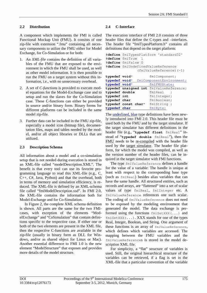
The execution interface of FMI 2.0 consists of three header files that define the C-types and –interfaces. The header file “fmiTypesPlatform.h” contains all definitions that depend on the target platform: #define fmiTypesPlatform "standard32" #define fmiTrue 1 #define fmiFalse 0 #define fmiUndefinedValueReference (fmiValueReference)(-1)

typedef void* fmiComponent; typedef void* fmiComponentEnvironment; typedef void* fmiFMUState; typedef unsigned int fmiValueReference; typedef double fmiReal ; typedef int fmiInteger; typedef char fmiBoolean; typedef const char* fmiString ; typedef char fmiByte;

The underlined, blue type definitions have been new-ly introduced into FMI 2.0. This header file must be used both by the FMU and by the target simulator. If the target simulator has different definitions in the header file (e.g., “typedef float fmiReal” in-stead of “typedef double fmiReal”), then the FMU needs to be re-compiled with the header file used by the target simulator. The header file plat-form, for which the model was compiled, as well as the version number of the header files, can be in-quired in the target simulator with FMI functions.

The type fmiValueReference defines a handle for the value of a variable: The handle is unique at least with respect to the corresponding base type (such as fmiReal) besides alias variables that can have the same handle. All structured entities, such as records and arrays, are “flattened” into a set of scalar values of type fmiReal, fmiInteger etc. A fmiValueReference references one such scalar. The coding of fmiValueReference does not need to be exposed by the modeling environment that generated the model. The data exchange is per-formed using the functions fmiSetXXX(...) and fmiGetXXX(...). XXX stands for one of the types Real, Integer, Boolean, and String. One argument of these functions is an array of fmiValueReference, which defines which variables are accessed. The mapping between the FMU variables and the fmiValueReferences is stored in the model de-scription XML file.

For simplicity, a “flat” structure of variables is used. Still, the original hierarchical structure of the variables can be retrieved, if a flag is set in the XML-file that a particular convention of the variable

Session 2A: FMI Standard I


names is used. For example, the Modelica variable name “pipe[3,4].T[14]” defines a variable which is the (3.4) element of an array of records “pipe” of vector T (“.” separates hierarchical levels and “[...]” defines array elements).

Header-file “fmiFunctionTypes.h” contains typedef definitions of all function prototypes of an FMU. When dynamically loading the DLL or shared object of an FMU, these definitions can be used to type-cast the function pointers to the respective func-tion definition. Example for a definition in this head-er file: typedef fmiStatus fmiSetTimeTYPE (fmiComponent, fmiReal); This header file was newly introduced in FMI 2.0 to ease the dynamic loading.

Finally, header file “fmiFunctions.h” contains the function prototypes of an FMU that can be accessed in simulation environments. This header file includes the other two header files from above. Example for a definition in this header file: DllExport fmiSetTimeTYPE fmiSetTime;

The goal is that both textual and binary represen-tations of models are supported and that several models using FMI might be present at link time in an executable (e.g., model A may use a model B). For this to be possible the names of the FMI-functions in different models must be different or function point-ers must be used. To support the first variant macros are provided in “fmiFunctions.h” to build the actual function names by using a function prefix that depends on how the FMU is shipped. Typically, FMU functions are used as follows: // FMU is shipped with C source code, // or with static link library #define FUNCTION_PREFIX MyModel_ #include "fmiFunctions.h" < usage of the FMU functions >

// FMU is shipped with DLL/SharedObject #define FUNCTION_PREFIX #include "fmiFunctions.h" < usage of the FMU functions >

If an FMU is shipped with C source code, or with a static link library, then a function that is defined as “fmiGetReal” is changed by the macros to the ac-tual function name “MyModel_fmiGetReal”. The function prefix is hereby defined in the XML file. A simulation environment can therefore construct the relevant function names by generating code for the actual function call. In case of a static link library, the name of the library is MyModel.lib on Windows, and libMyModel.a on Linux, in other words the function prefix attribute is used as library name.

If an FMU is shipped with a DLL/SharedObject, the constructed function name is “fmiGetReal”, in other words it is not changed. A simulation environ-ment will then dynamically load this library and will explicitly import the function symbols by providing the FMI function names as strings. The name of the library is MyModel.dll on Windows or MyModel.so on Linux, in other words the function prefix attribute is used as library name.

An FMU can be optionally shipped so that it ba-sically contains only the communication to another tool. This is particularly common for co-simulation tasks. In FMI 1.0, the function names are always pre-fixed with the model name and therefore a DLL/Shared Object has to be generated for every model. FMI 2.0 improves this situation since model names are no longer used as prefix in case of DLL/Shared Objects: Therefore one DLL/Shared Object can be used for all models in case of tool coupling.

3 New Features of FMI 2.0

In this section the main new features introduced by FMI 2.0 are sketched. Note, also many other minor improvements have been introduced, based on the experience in using FMI 1.0. Especially: • When instantiating an FMU, the simulation envi-

ronment must report the absolute path to the FMU resource directory also in Model Ex-change, in order that the FMU can read all of its resources (for example maps, tables, ...) inde-pendently of the "current directory" of the simu-lation environment where the FMU is used.

• Enumerations have an arbitrary (but unique) mapping to integers (in FMI 1.0, the mapping was automatically assigned to 1,2,3,...).

• When enabling logging, log categories can be defined, so that the FMU needs to only generate logs of the defined categories (in FMI 1.0, logs had to be generated for all log categories and they had to be filtered afterwards).

• Explicit alias/antiAlias variable definitions have been removed, to simplify the interface: If varia-bles of the same base type (such as fmiReal) have the same valueReference, they have identical values. A simulation environment may ignore this completely (this was not possible in FMI 1.0), or can utilize this information to more efficiently store results on file.

• Continuous state variables are explicitly listed as FMU variables, and an ordering is introduced for



them, as well as for inputs, and outputs in the XML file, in order that not an (arbitrary) order is selected by the simulation environment. This is essential, for example when linearizing an FMU, or when providing "sparsity" information (see below).

3.1 Unification of FMI for Model Exchange and Co-Simulation

In FMI 1.0 the Model Exchange and Co-Simulation interfaces were defined in two different documents. The XML-description and function definitions were slightly different. In version 2.0 both interfaces are combined in one document and unified. Now one FMU can implement both interfaces at the same time. The presence of the “ModelExchange” or “Co-Simulation” elements in the XML-description indi-cates which interface is implemented. Which inter-face is used by the environment is decided by calling the appropriate instantiation function (fmiInstan-tiateModel or fmiInstantiateSlave).

In this way the distributed use case (see [1]) which was applicable for Co-Simulation in FMI 1.0 only is supported in the Model Exchange case too. In this use case only the ability of a tool to evaluate the model equations is used, not its solver.

3.2 Classification of Interface Variables

Variables exposed by the FMU are now categorized in a slightly different way in FMI 2.0:

Attribute “causality” is an enumeration that defines the causality of the variable. Allowed values are: • parameter: An independent variable that must

be constant during simulation. • input: The variable value can be provided from

another model. • output: The variable value can be used by an-

other model. The algebraic relationship to the inputs is defined in element ModelStructure.

• local: Local variable that is calculated from other variables. It is not allowed to use the variable value in another model

Attribute “variability” is an enumeration that de-fines the time dependency of the variable, in other words it defines the time instants when a variable can change its value. Allowed values are: • constant: The value of the variable never chang-

es. • fixed: The value of the variable is fixed after

initialization. • tunable: The value of the variable is constant

between externally triggered events due to

changing variables with causality = "parameter" or "input" (see explanation below).

• discrete: The value of the variable is constant between internal events (= time, state, step events defined implicitly in the FMU).

• continuous: No restrictions on value changes. The new value “tunable” introduced in FMI 2.0 al-lows a modeling environment to expose independent parameters that can be manually “tuned” during sim-ulation (for example, during simulation a modeler might change the gain of a PID controller, or the load mass of a drive train in order to quickly improve the design).

“Tuning a parameter” during simulation does not mean to “change the parameter online” during simu-lation (since this might introduce Dirac impulses). Instead, this is a short hand notation for: 1. Stop the simulation at an event instant (usually, a

step event, in other words after a successful inte-gration step).

2. Change the values of the tunable parameters. 3. Compute all parameters that depend on the tuna-

ble parameters. 4. Resume the simulation using as initial values the

current values of all variables and the new values of the parameters.

With this interpretation, changing parameters online is “clean”, as long as these changes appear at an event instant.

3.3 Save and Restore of FMU state

An FMU has an internal state consisting of all values that are needed to continue a simulation. This inter-nal state consists especially of the values of the con-tinuous states, discrete states, iteration variables, pa-rameter values, input values, file identifiers and FMU internal status information. With newly intro-duced (optional) functions, the internal FMU state can be copied and the pointer to this copy is returned to the environment. The FMU state copy can be set as current FMU state, in order to continue the simu-lation from it. This feature introduced in FMI 2.0 can be for example used: • For iterative co-simulation master algorithms

(get the FMU state for every accepted communi-cation step; if the follow-up step is not accepted, restart co-simulation from this FMU state).

• For nonlinear Kalman filters (get the FMU state just before initialization; in every sample period, set new continuous states from the Kalman filter algorithm based on measured values; integrate to the next sample instant and inquire the predicted



continuous states that are used in the Kalman fil-ter algorithm as basis to set new continuous states).

• For nonlinear model predictive control (get the FMU state just before initialization; in every sample period, set new continuous states from an observer, initialize and get the FMU state after initialization. From this state, perform many simulations that are restarted after the initializa-tion with new input signals proposed by the op-timizer).

Furthermore, the FMU state can be serialized and copied into a byte vector. This can, for example be used to perform an expensive steady-state initializa-tion, copy the received FMU state in a byte vector and store this vector on file. Whenever needed, the byte vector can be loaded from file, can be deserial-ized and the simulation can be restarted from this FMU state, in other words from the steady-state ini-tialization.

3.4 Dependency Information

In FMI 1.0 only the dependencies of outputs on in-puts could be defined by the element “DirectDe-pendency” in the XML-description. In FMI 2.0 this information and the dependencies of outputs w.r.t. state variable and of derivatives w.r.t. inputs and state variables can be provided using the element “ModelStructure”. Under this element ordered lists of inputs, derivatives (with their associated state var-iable names) and outputs are provided. At each out-put and derivative additional attributes define the dependency on inputs and state variables. Not only the dependency itself but also the kind of dependen-cy is defined here. It can be indicated whether the dependency is nonlinear, fixed (the dependency is linear, the factor is constant after initialization) or discrete (the factor might change after events). Using this information a tool can decide at which stage of the solution process the respective entries of the Jacobian matrices are to be retrieved.

The dependency information of outputs can be utilized for detection of algebraic loops when FMUs are connected with other parts of a model. In addi-tion to that dependency information is necessary for usage of sparse matrix techniques on Jacobian matri-ces.

Assume for example that the following equations are defined:

1 1 22

2 2 1 2 1 3

3 3 1 3 1 2 3

1 2 3

( )( ) 3 2 3( , , , , )

( , )

x f xd x f x p x u udt

x f x x u u uy g x x

= + ⋅ ⋅ + ⋅ + ⋅

=

where u1 and u2 are continuous-time inputs (variabil-ity=”continuous”), u3 is a discrete-time input (var-iability=”discrete”), and p is a fixed parameter (variability=”fixed”). The structure of these equa-tions can then be defined optionally in the following way in the XML file: <ModelStructure> <Inputs> <Input name="u1"/> <Input name="u2"/> <Input name="u3"/> </Inputs> <Derivatives> <Derivative name="der(x1)" state="x1" stateDependencies="2" inputDependencies="" /> <Derivative name="der(x2)" state="x2" stateDependencies="1 2" stateFactorTypes ="nonlinear fixed" inputDependencies="1 3" inputFactorTypes ="fixed fixed" /> <Derivative name="der(x3)" state="x3" stateDependencies="1 3" /> </Derivatives> <Outputs> <Output name="y" stateDependencies="2 3" inputDependencies="" /> </Outputs> </ModelStructure>

3.5 Jacobian Matrices

Partial derivatives of FMU variables with respect to inputs or state variables (Jacobian matrices) are needed for implicit integration methods, for lineari-zation of FMUs, or for usage in extended Kalman filters. Especially for large models the numerical computation of Jacobian matrices is time consuming. For that reason FMUs can optionally provide func-tions to retrieve partial derivatives (complete Jacobi-ans) or directional derivatives of some variables w.r.t. some others.

The sparsity pattern defined under “ModelStrucu-tre” (see section above) can be utilized for efficient data storage and matrix operations on sparse Jacobi-ans. FMI does not define a specific storage schema. The calling environment is free to use its own sche-ma by the following approach. The environment has to provide a function pointer to a call back function setMatrix as argument of fmiGetPartialDe-



rivatives. The FMU calls this function to set re-spective matrix elements.

The FMU internally is free to use efficient nu-merical methods for Jacobian computation, use a symbolically deduced algorithm or automatic differ-entiation.

3.6 Precise Time Event Handling

The details of precise time event handling in FMI were still under discussion before the editorial dead-line of this paper. Hence we cannot present a detailed description here. The development work is compli-cated since several aspects have to be considered: • The synchronous features of Modelica 3.3 [2]

should be supported. • FMI should also be useable by tools that do not

support synchronous time event handling. • The time event handling is to be defined in a

way that allows backward compatible exten-sions.

3.7 Improved Unit Definitions

The unit definitions have been improved in FMI 2.0: The tool-specific unit-name can optionally be ex-pressed as function of the 7 SI base units and the SI derived unit “rad”. It is then possible to check units when FMUs are connected together (without stand-ardizing unit names as needed in FMI 1.0), or to convert variable values that are provided in different units (for the same physical quantity). In the specifi-caiton it is sketched how to utilize this information for connection checks, dimensional checks, or unit propagation. The trick is to treat the derived unit “rad” either as “rad” (for connection checks and unit propagation) or as “1” (for dimensional checks) de-pending on the situation.

4 Examples

In this section two examples are shown that demon-strate the structure of the XML file and especially how FMUs can be connected together. The use case is an often occurring situation where two FMUs shall be connected that have a mechanical interface.

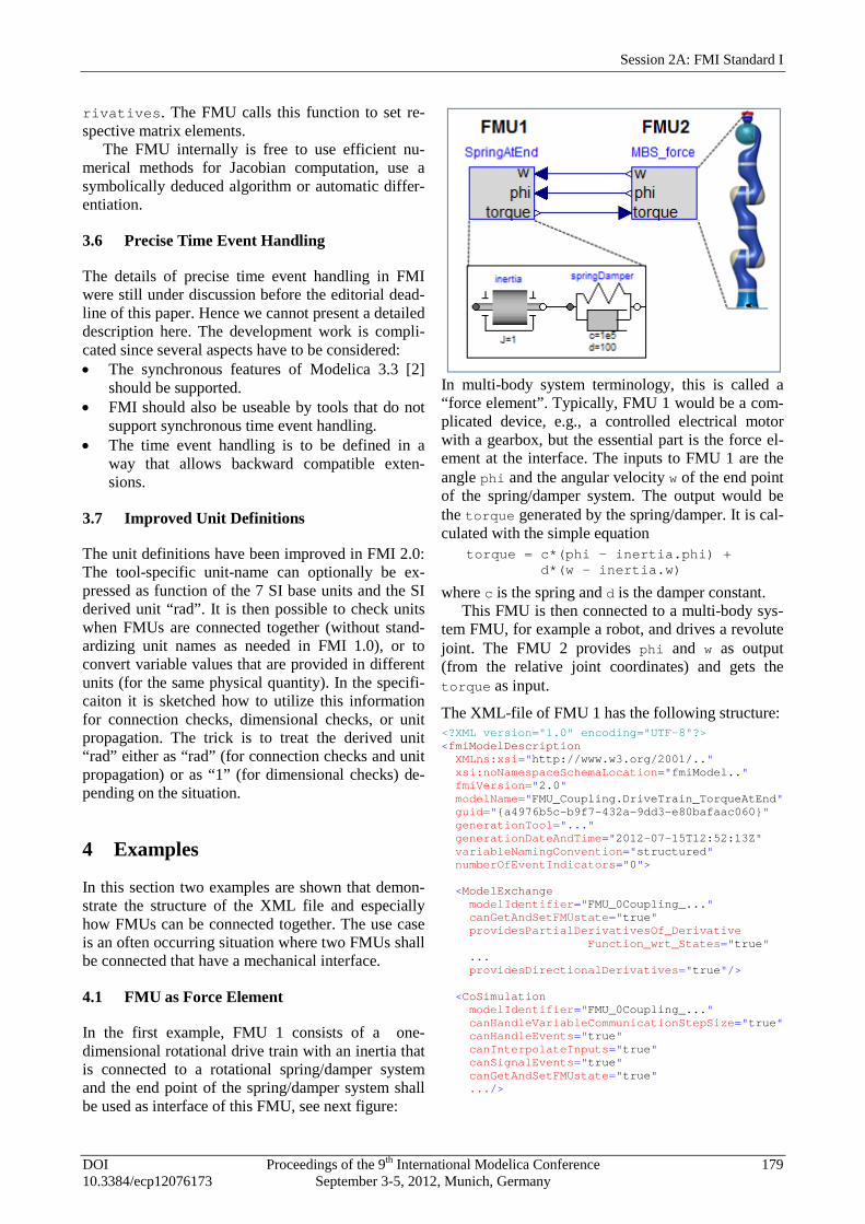
4.1 FMU as Force Element

In the first example, FMU 1 consists of a one-dimensional rotational drive train with an inertia that is connected to a rotational spring/damper system and the end point of the spring/damper system shall be used as interface of this FMU, see next figure:

In multi-body system terminology, this is called a “force element”. Typically, FMU 1 would be a com-plicated device, e.g., a controlled electrical motor with a gearbox, but the essential part is the force el-ement at the interface. The inputs to FMU 1 are the angle phi and the angular velocity w of the end point of the spring/damper system. The output would be the torque generated by the spring/damper. It is cal-culated with the simple equation torque = c*(phi - inertia.phi) + d*(w – inertia.w)

where c is the spring and d is the damper constant. This FMU is then connected to a multi-body sys-

tem FMU, for example a robot, and drives a revolute joint. The FMU 2 provides phi and w as output (from the relative joint coordinates) and gets the torque as input.

The XML-file of FMU 1 has the following structure: <?XML version="1.0" encoding="UTF-8"?> <fmiModelDescription XMLns:xsi="http://www.w3.org/2001/.." xsi:noNamespaceSchemaLocation="fmiModel.." fmiVersion="2.0" modelName="FMU_Coupling.DriveTrain_TorqueAtEnd" guid="{a4976b5c-b9f7-432a-9dd3-e80bafaac060}" generationTool="..." generationDateAndTime="2012-07-15T12:52:13Z" variableNamingConvention="structured" numberOfEventIndicators="0"> <ModelExchange modelIdentifier="FMU_0Coupling_..." canGetAndSetFMUstate="true" providesPartialDerivativesOf_Derivative Function_wrt_States="true" ... providesDirectionalDerivatives="true"/> <CoSimulation modelIdentifier="FMU_0Coupling_..." canHandleVariableCommunicationStepSize="true" canHandleEvents="true" canInterpolateInputs="true" canSignalEvents="true" canGetAndSetFMUstate="true" .../>



<UnitDefinitions> <Unit name="N.m"> <BaseUnit kg="1" m="2" s="-2"/> </Unit> </UnitDefinitions> <TypeDefinitions> <SimpleType name="Modelica.SIunits.Torque"> <Real quantity="Torque" unit="N.m"/> </SimpleType> ... </TypeDefinitions> <DefaultExperiment startTime="0.0" stopTime="1.0" tolerance="0.0001"/> <ModelVariables> <ScalarVariable name="torque" valueReference="335544320" description="Torque in flange" causality="output"> <Real declaredType= "Modelica.Blocks.Interfaces.RealOutput" unit="N.m"/> ... </ModelVariables> <ModelStructure> <Inputs> <Input name="phi"/> <Input name="w" derivative="1"/> </Inputs> <Derivatives> <Derivative name="der(inertia.phi)" state="inertia.phi" stateDependencies="2" inputDependencies=""/> <Derivative name="der(inertia.w)" state="inertia.w"/> </Derivatives> <Outputs> <Output name="torque" inputDependencies="1 2" inputFactorKinds="fixed fixed"/> </Outputs> </ModelStructure> </fmiModelDescription>

Most of the elements should be self-explanatory. The interesting part for the connection is element “ModelStructure” at the end. Output torque de-pends on the first and the second input, i.e. on phi and w. Furthermore, the attributes fixed define that the inputs enter the equation for the output with fixed linear factors:

torque = p1*phi + p2*w + f(..)

where p1 and p2 are constants that are fixed after initialization. Additionally, for input w the attribute derivative = ”1” is defined. The meaning is that w is the derivative of the first input, i.e. of phi. This derivative information for inputs and outputs is es-sential in order that a coupling tool can check that an input is really the derivatives of another input by checking the derivative attributes of the outputs from another FMU.

The XML-file for FMU 2 looks similar. We will concentrate only on the ModelStructure element: <ModelStructure> <Inputs> <Input name="torque"/> </Inputs> <Derivatives> ... <Outputs> <Output name="phi" stateDependencies="1" inputDependencies=""/> <Output name="w" derivative="1" stateDependencies="2" inputDependencies=""/> </Outputs> </ModelStructure>

The important point is that empty inputDependen-cies lists are defined for the outputs. This means that the outputs phi and w do not directly depend on the input torque. As a result, when connecting FMU 2 to FMU 1, the outputs phi and w are provided by FMU 2. FMU 1 computes its output torque that is an input to FMU 2. Since the FMU 2 outputs do not depend on this input, there is no algebraic loop and the computation is simple.

4.2 FMUs with Coupling Constraint

The second example is the more often occurring case, but is more involved. FMU 1 is again a one-dimensional rotational drive train, but ends this time with a rotational inertia, see next figure:

Since FMU 1 is connected to a joint of FMU 2, the coupling leads to a constraint equation that states that the angle of the revolute joint of FMU 2 is identical to the angle of inertia2 in FMU 1. It is well-known that such a model cannot be transformed by purely algebraic transformations into a state space



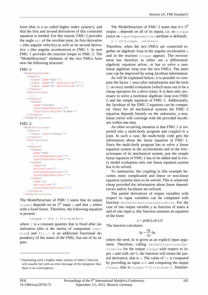
form (this is a so called higher index system2), and that the first and second derivatives of this constraint equation is needed. For this reason, FMU 2 provides the angle phi of the revolute joint, its first derivative w (the angular velocity) as well as its second deriva-tive a (the angular acceleration) to FMU 1. In turn FMU 1 provides the reaction torque to FMU 2. The “ModelStructure” elements of the two FMUs have now the following structure:

FMU 1: <ModelStructure> <Inputs> <Input name="phi"/> <Input name="w" derivative="1"/> <Input name="a" derivative="2"/> </Inputs> <Derivatives> ... <Outputs> <Output name="torque" inputDependencies="3" inputFactorKinds="fixed"/> </Outputs> </ModelStructure>

FMU 2: <ModelStructure> <Inputs> <Input name="torque"/> </Inputs> <Derivatives> ... <Outputs> <Output name="phi" stateDependencies="1" inputDependencies=""/> <Output name="w" derivative="1" stateDependencies="2" inputDependencies=""/> <Output name="a" derivative="2" stateDependencies="1"/> </Outputs> </ModelStructure>

The ModelStructure of FMU 1 states that its output torque depends on its 3rd input a and that a enters with a fixed factor. Therefore, the following equation is present: torque = J*a + f1(<states>)

where J is a constant quantity that is fixed after ini-tialization (this is the inertia of component iner-tia2) and f1(..) is an additional functional de-pendency of the states of the FMU, but not of its in-puts.

2 Simulating such a higher index system of index 3 directly

will usually fail with an error message of the integrator that there is no convergence.

The ModelStructure of FMU 2 states that it’s 3rd output a depends on all of its inputs, i.e. on torque (since no inputDependencies attribute is defined):

a = f2(torque, <states>)

Therefore, when the two FMUs are connected to-gether an algebraic loop in the angular acceleration a and in the reaction torque appears. The environ-ment has therefore to either use a differential-algebraic equation solver, or has to solve a non-linear algebraic loop over the two FMUs. The latter case can be improved by using Jacobian information:

As will be explained below, it is possible to com-pute the factor J once after initialization and the term f1 at every model evaluation (which turns out to be a cheap operation for a drive train). It is then only nec-essary to solve a nonlinear algebraic loop over FMU 2 and the simple equation of FMU 1. Additionally, the Jacobian of the FMU 2 equation can be comput-ed. Since for all mechanical systems the FMU 2 equation depends linearly on the unknowns, a non-linear solver will converge with the provided Jacobi-ans within one step.

An often occurring situation is that FMU 1 is im-ported into a multi-body program and coupled to a joint. In such a case, the multi-body code gets the information about the linear equation of FMU 1. Since the multi-body program has to solve a linear equation system in the accelerations and in the forc-es/torques of its mechanical system, just the simple linear equation of FMU 1 has to be added and in eve-ry model evaluation only one linear equation system has to be solved.

To summarize, the coupling in this example be-comes more complicated and linear or non-linear equation systems have to be solved. This is relatively cheap provided the information about linear depend-encies and/or Jacobians are utilized.

The partial derivatives of output variables with respect to input variables can be computed with function fmiGetDirectionalDerivative. For the case of one output variable y as function of states x and of one input u, this function assumes an equation of the form:

( ( ), ( ), )=y g t u t tx The function calculates:

∂∆ = ∆

∂gy uu

where the seed Δu is given as an explicit input argu-ment. Therefore, calling fmiGetDirectionalDe-rivative for the output torque with respect to in-put a and with Δa=1, the function will return the par-tial derivative, that is J. The value of f1 is computed by providing an input a=0 and computing the output torque, that is torque = f1(<states>). Similari-



ly, the partial derivative of the FMU 2 equation can be computed.

As a final remark: When FMU 1 is modeled in Modelica, then the derivative relationships between the inputs of the FMU must be defined, otherwise a Modelica translator cannot process the model. There is no direct Modelica language element available to define this. However, with component Modeli-ca.Mechanics.Rotational.Sources.Move from the Modelica Standard library this relationship is ex-pressed (based on language elements to express that a function is a derivative of another function).

5 Increasing Quality of FMI Imple-mentations

The FMI project provides an infrastructure to in-crease the quality and compatibility of implementa-tions in different tools. A repository of FMUs gener-ated by different tools and reference results are pub-lically available at the svn server:

https://svn.fmi-standard.org/fmi/trunk/Test_FMUs In this way tool vendors are able to cross check their implementations in an easy way. We hereby would like to ask tool vendors that export FMUs, to provide FMUs of their tools by sending an email with the FMUs to [email protected].

Additionally, the Modelica Association contract-ed the development of an open source FMI compli-ance checker. This tool is now available for FMI 1.0 in source code, and as executable for Windows and Linux under the svn address from above. It will be available for FMI 2.0 soon after FMI 2.0 is released.

6 FMI Usage

FMI is used in industrial and scientific projects by several companies and research institutions:

In all new gearbox projects for Mercedes-Benz passenger cars FMI is used for software-in-the-loop simulations [3]. Control software and FMUs coming from different modeling environments run in closed-loop in the virtual ECU tool Silver on Windows PC in order to validate, test and debug control software.

Before FMI, vehicle models had to be imported through various vendor and version specific import procedures into Silver. This was expensive and error prone. Thanks to the FMI, these bridges have now been replaced by a uniform import interface, increas-ing thereby the cost-benefit ratio of simulation in this domain.

In mechatronic gearshift simulations for commer-cial vehicles at Daimler AG FMI is utilized twice [4]. At first controller software is connected to a de-tailed 1D powertrain model in SimulationX. After-wards this model is exported as FMU and imported to the multibody system simulation tool Simpack. There it is connected to a detailed truck model. This allows the holistic simulation and optimization of the shifting comfort.

At IFP Energies Nouvelles, FMI for Model Ex-change is used to parallelize the execution of com-plex internal combustion engine models in the tool xMOD (see [5]). The models have around 100 - 300 state variables, with integration step-sizes that can reach some microseconds. Their use is mainly in-dented to validate engine controls. The final target is to enable the execution in real-time, for hardware in the loop simulations.

In [6], an algorithm is implemented for deriva-tive-free optimization implemented in Python and applied to parameter optimization of FMUs is intro-duced. The FMUs are loaded and simulated using the PyFMI package (http://www.pyfmi.org). The opti-mization algorithm is applied to a Volvo truck en-gine to identify model parameters based on meas-urement data from a test cycle.

In [7] the FMI based co-simulation master from Fraunhofer is used to develop, implement and test sophisticated algorithms for the co-simulation of FMUs generated by Dymola.

Dassault Systèmes uses FMI for academically trainings. Student teams work with CATIA V6 and define both a 3D CATIA representation of a NXT robot as well as the controller software. Practically, the real robot has sensors and actuators and is piloted from a smartphone remote command, while the FMU based logical control is executed in a CATIA ses-sion. All these items are FMI and Bluetooth connect-ed.

The solution has been delivered to Georgia Insti-tute of Technology and University of Detroit Mercy (US High Schools), also related to a cooperation with Ford Motors Foundation.

In the field of modeling and simulation of build-ing energy systems FMI is also used. In [8] FMI is utilized to connect a building model with a Modelica model of the heating system.

In 2012, the International Energy Agency, under the implementing agreement on Energy Conserva-tion in Buildings and Community Systems, approved the five-year Annex 60 proposal "New generation computational tools for building and community en-ergy systems based on the Modelica and Functional Mockup Interface standards." Eleven countries are expected to participate in sharing, developing and



https://svn.fmi-standard.org/fmi/trunk/Test_FMUs

mailto:[email protected]

http://www.pyfmi.org/

deploying free open-source contributions for model-ing and simulation of energy systems of buildings and communities, based on Modelica and Functional Mockup Interface standard.

The Lawrence Berkeley National Laboratory (LBNL) released an FMI for co-simulation import interface in version 7.1 of the EnergyPlus building simulation program. Work is also in progress to ex-port EnergyPlus as a FMU for Co-Simulation. UC Berkeley and LBNL have been developing JFMI, a Java Wrapper for FMI for Co-Simulation and Model Exchange. JFMI will be used to integrate an FMI import interface in Ptolemy II, a software environ-ment for design and analysis of heterogeneous sys-tems.

The Institute for the Sustainable Performance of Buildings has been developing a web-based eLearn-ing tool, Learn Green Buildings (http://learngreenbuildings.org), in which a Web in-terface communicates with an FMU for Co-Simulation that computes the dynamic response of building energy and control systems. The tool will allow students to interactively operate a simulated, realistic building system, to test energy-saving measures and to explore the effects of faults in equipment and controls.

7 Conclusions and Outlook

FMI is an established standard for Model Exchange and Co-Simulation. The upcoming version 2.0 im-proves the compatibility of implementations by a clarified specification. New features increase usabil-ity and performance especially for large models.

This version will be stable for the next years. If necessary, minor backwards compatible releases will be available to improve and clarify the specification and to support new features. Current development tasks are the exchange of structured data and arrays of variable size and support of the new synchronous features of the Modelica language [2].

The further development of FMI is organized un-der the hood of the Modelica Association. The FMI Modelica Association Project is of course open for non Modelica tool vendors and organizations. From the 16 members of the FMI Steering Committee and Advisory Group, only five are Modelica Tool ven-dors.

Companies and organizations which are interest-ed to contribute to FMI development or request fea-tures are invited to contact the FMI project via [email protected].

8 Acknowledgements The authors wish to thank all the contributors to the FMI specification (see Annex). Parts of this work were supported by the German BMBF (Förderkennzeichen: 01IS08002), the French DGCIS, and the Swedish VINNOVA (funding num-ber: 2008-02291) within the ITEA2 MODELISAR project (http://www.itea2.org/project/result/download/result/5533) The authors appreciate the partial funding of this work.

9 References

[1] T. Blochwitz, M. Otter, M. Arnold, C. Bausch, C. Clauß, H.Elmqvist, A. Junghanns, J. Mauss, M. Monteiro, T. Neidhold, D. Neumerkel, H. Olsson, J.-V. Peetz, S. Wolf: The Functional Mockup Inter-face for Tool independent Exchange of Simulation Models. 8th International Modelica Conference. Dresden 2011. Download: http://www.ep.liu.se/ecp/063/013/ecp11063013.pdf

[2] Modelica Association: Modelica – A Unified Ob-ject-Oriented Language for Systems Modeling. Language Specification, Version 3.3. May 9, 2012.

[3] E. Chrisofakis, A. Junghanns, C. Kehrer, A. Rink: Simulation-based development of automotive con-trol software with Modelica. 8th International Modelica Conference. Dresden 2011. Download: http://www.ep.liu.se/ecp/063/001/ecp11063001.pdf

[4] A. Abel, T. Blochwitz, A. Eichberger, P. Hamann, U. Rein: Functional Mock-up Interface in Mecha-tronic Gearshift Simulation for Commercial Ve-hicles. 9th International Modelica Conference. Mu-nich, 2012.

[5] Abir Ben Khaled, Mongi Ben Gaid, D. Simon, G. Font: Multicore simulation of powertrains using weakly synchronized model partitioning. Accept-ed for 2012 IFAC Workshop on Engine and Power-train Control, Simulation and Modeling. Rueil-Malmaison, 2012

[6] S. Gedda, C. Andersson, J. Åkesson, S. Diehl: De-rivative-free Parameter Optimization of Func-tional Mock-up Units. 9th International Modelica Conference. Munich, 2012.

[7] T. Schierz, M. Arnold, C. Clauss: Co‐simulation with Communication Step Size Control in an FMI Compatible Master Algorithm. 9th International Modelica Conference. Munich, 2012.

[8] S. Burhenne, M. Pazold, F. Antretter, F. Ohr, S. Her-kel, J. Radon: WUFI Plus Therm: Co-Simulation unter Verwendung von Modelica Modellen. Presentation at the Symposium „Integrale Planung und Simulation in Bauphysik und Gebäudetechnik.“ Dresden, March 2012.



http://learngreenbuildings.org/

mailto:[email protected]

http://www.itea2.org/project/result/download/result/5533

http://www.itea2.org/project/result/download/result/5533

http://www.ep.liu.se/ecp/063/013/ecp11063013.pdf

http://www.ep.liu.se/ecp/063/001/ecp11063001.pdf

Annex Members of the FMI Modelica Association Project:

The Steering Committee is open for additional members that actively support FMI. Requirements: Must have (a) participated at least at two FMI meetings in the last 24 months, (b) must either provided the FMI standard or part of it in a commercial or open source tool, and/or must actively use FMI in industrial projects, (c) the Steering Committee members agree with qualified majority.

The Advisory Committee is open for additional members that proofed to actively support FMI. Require-ments: Must have (a) participated at least at two FMI meetings in the last 24 months, and (b) the Steering Committee members agree with qualified majority.

Contributors to the FMI 2.0 Specification: The following persons participated at FMI 2.0 design meetings and contributed to the discussion (alphabeti-cal list):

Martin Arnold, University Halle, Germany Johan Akesson, Modelon, Sweden Mongi Ben-Gaid, IFP, France Torsten Blochwitz, ITI GmbH Dresden, Germany Christoph Clauss, Fraunhofer IIS EAS, Germany Alex Eichberger, SIMPACK AG, Germany Hilding Elmqvist, Dassault Systèmes AB, Sweden Markus Friedrich, SIMPACK AG, Germany Peter Fritzson, PELAB, Sweden Andreas Junghanns, QTronic, Germany Petter Lindholm, Modelon, Sweden Kristin Majetta, Fraunhofer IIS EAS, Germany Sven Erik Mattsson, Dassault Systèmes AB, Sweden Jakob Mauss, QTronic, Germany Dietmar Neumerkel, Daimler AG, Germany Peter Nilsson, Dassault Systèmes AB, Sweden Hans Olsson, Dassault Systèmes AB, Sweden Martin Otter, DLR (RMC-SR), Germany Bernd Relovsky, Daimler AG, Germany Tom Schierz, University Halle, Germany Bernhard Thiele, DLR (RMC-SR), Germany Antoine Viel, LMS International, Belgium

The following people contributed with comments (alphabetical list): Peter Aaronsson, MathCore, Sweden Bernhard Bachmann, University of Bielefeld, Germany Iakov Nakhimovski, Modelon, Sweden Andreas Pfeiffer, DLR (RMC-SR), Germany

Project Leader Torsten Blochwitz (ITI GmbH Dresden, Germany) Steering Committee Atego, Daimler, Dassault Systèmes, IFP EN, ITI, LMS, Modelon, QTronic,

SIMPACK Advisory Board Armines, DLR, Fraunhofer (IIS/EAS, First, SCAI), Open Modelica Consortium,

TWT, University of Halle Guests Altair Engineering, Berkeley University, Bosch, ETAS, Siemens, Equa Simula-

tion



Documents

Functional Mockup Interface 2.0: The Standard for Tool independent