Fuselage boundary-layer refraction of fan tones1

radiated from an installed turbofan aero-enginea)2

James Gaffney and Alan McAlpineb)

Institute of Sound and Vibration Research, University of Southampton, Southampton, SO17 1BJ, UK

Michael J. Kingan

Department of Mechanical Engineering, University of Auckland, Auckland, New Zealand

3

February 6, 20174

a) Part of this work was presented in “Sound radiation of fan tones from an installed turbofan aero-engine: fuselage

boundary-layer refraction effects”, Proceedings of the 22nd AIAA/CEAS Aeroacoustics conference, Paper no. AIAA-

2016-2878, Lyon, France, 30 May–1 June 2016.b) Author to whom correspondence should be addressed. Electronic mail: am@isvr.soton.ac.uk

1

Abstract5

A distributed source model to predict fan tone noise levels of an installed turbofan aero-engine6

is extended to include the refraction effects caused by the fuselage boundary layer. The model7

is a simple representation of an installed turbofan, where fan tones are represented in terms8

of spinning modes radiated from a semi-infinite circular duct, and the aircraft’s fuselage is9

represented by an infinitely long, rigid cylinder. The distributed source is a disc, formed by10

integrating infinitesimal volume sources located on the intake duct termination. The cylinder is11

located adjacent to the disc. There is uniform axial flow, aligned with the axis of the cylinder,12

everywhere except close to the cylinder where there is a constant thickness boundary layer. The13

aim is to predict the near-field acoustic pressure, and in particular to predict the pressure on the14

cylindrical fuselage which is relevant to assess cabin noise. Thus no far-field approximations15

are included in the modelling. The effect of the boundary layer is quantified by calculating the16

area-averaged mean square pressure over the cylinder’s surface with and without the boundary17

layer included in the prediction model. The sound propagation through the boundary layer is18

calculated by solving the Pridmore-Brown equation. Results from the theoretical method show19

that the boundary layer has a significant effect on the predicted sound pressure levels on the20

cylindrical fuselage, owing to sound radiation of fan tones from an installed turbofan aero-21

engine.22

2

I. Introduction23

Organisations such as the International Civil Aviation Organisation (ICAO) and the American Fed-24

eral Aviation Administration (FAA) oversee noise certification of civil aircraft, including setting25

stringent targets for the reduction of noise. To aid meeting these requirements, practical and reli-26

able noise prediction methods are an essential part of the research and development toolkit. This27

paper presents a new theoretical method to predict the sound radiation of fan tones from an installed28

turbofan aero-engine, focussing on the prediction of the fuselage sound pressure levels (SPL), and29

how these levels are affected by refraction effects caused by the fuselage boundary layer.30

Noise from aero-engines has a major impact on communities around airports as well as the pas-31

sengers and crew aboard the aircraft. At take-off and cruise conditions the aero-engines are the32

dominant source of noise from civil aircraft. A turbofan engine represents a very complex noise33

source, and as such the noise generation and radiation mechanisms are difficult to model accurately.34

The complexity is compounded by the presence of the airframe. Consequently, turbofan noise mod-35

els often predict the sound radiated into free space. However, the radiated noise is affected by the36

whole aircraft, including the fuselage, wings, high-lift devices, landing gear etc. How the radiated37

acoustic field is affected by interaction with the airframe is referred to as installation acoustics.38

This paper will focus on prediction of the sound pressure levels on an aircraft fuselage. The39

key aim is to develop a simple installation acoustics method based on a canonical problem: how40

to predict the pressure field due to a source located near an infinite, rigid cylinder. The basis of41

the method is a classical problem: acoustic scattering by a cylinder. The analytical solution for42

the acoustic field due to a point source located adjacent to an infinite cylinder is given in the text43

by Bowman, Senior and Uslenghi (Chapter 2, §2.5.2, pp. 126–127) [1] . Simplifications in the44

3

geometry and the mean flow must be made to use analytical techniques, but these do not necessarily45

curtail the usefulness of the solutions. In this case, the aircraft’s fuselage is represented by the46

cylinder. Also, except close to the fuselage, the flow is assumed to be uniform and its direction is47

aligned with the axis of the cylinder.48

Of principal interest in this current work is the effect of the fuselage boundary layer. One of the49

earliest examples of work in this area is by Hanson [2] who studied the problem of a point source50

over a rigid flat plate with a boundary layer. Subsequently, Hanson and Magliozzi [3] examined51

the more advanced and realistic problem of an open-rotor source located adjacent to a cylindrical52

fuselage, and with the inclusion of the fuselage boundary layer. This type of model also has been53

investigated by Lu [4], who utilized a point source model. Most recently Brouwer [5] studied the54

effects of a boundary layer on the near side of a cylinder for an open-rotor type source. The model55

was extended to the far-field where there was a modest effect on the free-field predictions caused by56

the boundary layer.57

Historically, these type of theoretical methods for fuselage installation acoustics have focused58

on open-rotor noise sources. More recently, the procedure given by Hanson and Magliozzi was59

followed by McAlpine, Gaffney and Kingan [6] to develop a scattering model for a realistic tur-60

bofan source located adjacent to an infinitely long, rigid cylindrical fuselage. A disc source was61

formulated so that the source distribution was representative of sound radiation for a ducted fan62

noise source. The source is a disc formed by integrating infinitesimal volume sources located on63

the duct termination. The source strength (volume velocity) is proportional to the axial component64

of the particle velocity at the duct termination, following the Kirchhoff approximation. Originally65

Tyler and Sofrin [7] used this approach to construct a Rayleigh integral in terms of a non-uniform66

velocity distribution across the duct termination. The particle velocity is given by the well-known67

4

‘spinning’ mode solution for sound propagation in a cylindrical waveguide. Thus, tones generated68

by a ducted fan are modelled in terms of spinning modes propagating inside the intake duct. This69

approach neglects diffraction effects at the duct lip, but Hocter [8] has shown that these are largely70

insignificant for sound radiation up to approximately 70 degrees relative to the axis of the duct.71

Accordingly, the scattering model is only valid for sound radiation in the forward arc.72

This paper extends recent work published in Ref. [6]. The key advancement is the inclusion of73

the effect of boundary-layer refraction in the modelling. The cylindrical fuselage is in the near-field74

of the source. Thus it is not valid to use a far-field approximation of the sound field radiated by the75

source, a la the far-field solution of the Rayleigh integral for a circular disc source. In Ref. [6] the76

ducted fan noise source was incorporated into a cylinder scattering model with uniform mean flow77

everywhere. In this paper, the same method for a ducted fan noise source is extended to include78

refraction effects caused by a boundary layer of constant thickness on the cylindrical fuselage.79

II. Theory80

A. Fuselage scattering81

The acoustic pressure field owing to a fan tone radiated from an intake duct located adjacent to82

an infinitely long, rigid cylindrical fuselage was derived in McAlpine, Gaffney and Kingan [6]. A83

sketch of the problem set-up is shown in Figure 1; also shown is some of the nomenclature used in84

the solution, and the Cartesian reference frames for the source (x, y, z) and the cylinder (x, y, z).85

The equivalent cylindrical polar coordinate reference frames are (r, φ, z) for the source and (r, φ, z)86

for the cylinder. There is a subsonic uniform mean flow, Mach number M∞, directed in the negative87

z-direction. The total pressure field (sum of the incident and scattered fields) is calculated in the88

5

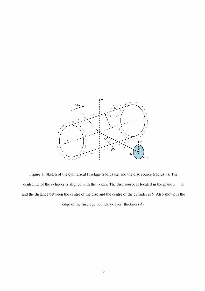
Figure 1: Sketch of the cylindrical fuselage (radius a0) and the disc source (radius a). The

centreline of the cylinder is aligned with the z-axis. The disc source is located in the plane z = 0,

and the distance between the centre of the disc and the centre of the cylinder is b. Also shown is the

edge of the fuselage boundary-layer (thickness δ).

6

forward arc z > 0.89

From Ref. [6], the time-harmonic total pressure pt(r, φ, z, t

)= pt

(r, φ, z

)exp iω0t, is ex-90

pressed in terms of a Fourier series, and each Fourier harmonic is itself expressed in terms of an91

inverse Fourier transform. The result from Ref. [6] can be written in non-dimensional form as92

pt(r, φ, z

)=

1

(2π)2

∞∑n=−∞

∫ ∞−∞

(pin + psn

)e−ikz zdkz

e−inφ , (1)

where the incident field93

pin (r, kz) = π2ξlqPlq(−1)l+ne−i(l−n)β (k0 + kzM∞) ΨlqH(2)l−n(Γ0b)Jn(Γ0r) , (2)

and the scattered field94

psn (r, kz) = −π2ξlqPlq(−1)l+ne−i(l−n)β (k0 + kzM∞) Ψlq

H(2)l−n(Γ0b)J

′n(Γ0)

H(2) ′n (Γ0)

H(2)n (Γ0r) , (3)

where · denotes variables which have been Fourier transformed. The Bessel function of the first95

kind of order ` is denoted by J`, and the Hankel function of the second kind of order ` is denoted96

by H(2)` . The ′ denotes differentiation with respect to the function’s argument. Full details are in97

McAlpine, Gaffney and Kingan [6].98

In Equations (1–3), all the variables have been made non-dimensional by taking the reference99

length scale equal to the radius of the cylinder, a0, the reference velocity equal to the speed of100

sound, c0, and the reference density equal to the ambient density, ρ0. Then the pressure is scaled by101

ρ0c20.102

The fan tone source is modelled by the time-harmonic spinning mode (l, q), where l denotes the103

azimuthal order and q denotes the radial order. The mode has amplitude Plq, wavenumber k0 and104

angular frequency ω0. The dispersion relationship for the mode is105

kz2lq + κ2

lq =(k0 + kzlqM∞

)2, (4)

7

and the mode amplitude coefficient106

ξlq =kzlq(

k0 + kzlqM∞) . (5)

The term Ψlq is found by integration over the disc source. This integral can be evaluated exactly.107

For non-plane-wave excitation, for r > a108

Ψlq =

Γ0a

(κ2lq−Γ20)

Jl(κlqa)J′l(Γ0a) if Γ0 6= κlq

12

(a2 − l2

κ2lq

)J2l (κlqa) if Γ0 = κlq

, (6)

and for plane-wave excitation109

Ψ01 =

− a

Γ0J′0(Γ0a) if Γ0 6= 0

12a2 if Γ0 = 0

. (7)

Similar to Equation (4), the ‘radial’ wavenumber of the radiated field, Γ0, is given by110

Γ20 = (k0 + kzM∞)2 − kz2 , (8)

and equals zero at111

k−z = − k0

1 +M∞and k+

z =k0

1−M∞. (9)

From Equations (8) and (9), the wavenumber Γ0 is defined as112

Γ0 = −i√

1−M2∞

√−i (kz − k+

z )√

i (kz − k−z ) , (10)

on taking the principal value of the square root. In the range k−z < kz < k+z , the wavenumber Γ0113

is real and positive, and corresponds to wavenumbers which radiate to the far field. Outside of this114

range, Γ0 = −iγ0 where γ0 =√k2z − (k0 + kzM∞)2 > 0. This wavenumber range corresponds to115

an evanescent field. Accordingly, the integration of the inverse Fourier transform in Equation (1) is116

split into three parts as shown in Table 1. Moreover, the definition of Γ0 given by Equation (10) also117

8

LabelLimits

Γ0

lower higher

I1 −∞ k−z −iγ0

I2 k−z k+z

√(k0 +M∞kz)2 − k2

z

I3 k+z ∞ −iγ0

Table 1: Breakdown of the inverse Fourier transform integral in Equation (1). The full integral is

given by I1 + I2 + I3. The value of the wavenumber Γ0 in each region is specified.

prescribes the appropriate location of the branch cuts from points k−z and k+z such that on taking the118

inverse Fourier transform the radiation conditions will be correct.119

Measured relative to the axis of the intake duct (z), as the source Helmholtz number k0a in-120

creases, the mode and propagation angles also increase. There are several ways that can be used to121

predict the radiation angle of the principal lobe. One estimate is given by the mode (or phase) angle,122

which can be calculated directly from the dispersion relationship (4). Rice [9] derived an alternative123

expression for the radiation angle, viz.124

cos θ =√

1−M2∞

1− 1/ζ2

1−M2∞ (1− 1/ζ2)

1/2

, (11)

where ζ is the cut-off ratio125

ζ =k0

kzlq√

1−M2∞. (12)

This result is commonly used to predict the principal radiation angle in the presence of flow.126

Alternatively the radiation angle can be found numerically by direct computation of the direc-127

tivity function. For the disc source, the radiated pressure field, expressed in the source coordinates128

9

(r, φ, z), is given by129

pi (r, φ, z) =ξlqPlq

4

∫ ∞−∞

(k0 + kzM∞) Ψlq H(2)l (Γ0r) e−ikzz dkz e−ilφ , (13)

at field points r > a. Equation (13) is taken from McAlpine, Gaffney and McAlpine ([6], Eq. (20)).130

The location on the cylinder’s surface where the SPL is at a maximum can be estimated utilizing131

the radiation angle of the principal lobe and simple geometry. An example of this is shown in132

Figure 2. Numerical evaluation of the radiation angle provides the closest estimate to the location133

of the maximum SPL on the cylinder. This is because the cylinder is located in the near field,134

whereas the analytic formulas for the mode and propagation angles are valid in the far field.135

Figure 2: Normalised total SPL on the surface of the cylinder. The location of the maximum value

of the SPL is shown by the blue dot. Predictions of this point obtained using (i) mode (phase)

angle, (ii) radiation angle (11), or (iii) numerical evaluation of the near-field (in the absence of the

cylinder), are also shown. Key: (i) magenta dot; (ii) black dot; (iii) green dot. Other relevant

parameters in this example are (l, q) = (2, 1), k0a = 5, b = 3 and M∞ = 0.5.

B. Fuselage scattering including boundary-layer refraction136

The technique to include the boundary layer in the method is outlined in this section. A sketch of137

the cylindrical fuselage, including the constant-thickness boundary layer is shown in Figure 1. The138

10

velocity profile Mz is given by139

Mz =

M(r) 1 < r ≤ 1 + δ

M∞ 1 + δ < r

, (14)

where δ is the non-dimensional thickness of the boundary-layer, and M(r) is the boundary-layer140

Mach number profile which is assumed to be a smooth, monotonically increasing function. Note141

that the non-dimensional radius of the fuselage is unity.142

Outside the boundary layer, where the source is located, there is uniform flow and the acoustic143

pressure field is found by solving the convected wave equation. Inside the boundary layer region,144

the pressure field, pbl, will satisfy the Pridmore-Brown equation.145

An inviscid, compressible, isentropic, perfect gas flow is assumed. Additionally, the mean flow146

is assumed to be axisymmetric and parallel, with constant mean density and sound speed profiles in-147

side the boundary layer. The appropriate field equation for the pressure which captures the refractive148

effects of the sheared mean flow is given by149

D0

Dt

(D2

0pblDt2

−∇2pbl

)− 2

dM

dr

∂2pbl∂r∂z

= 0 . (15)

In order to determine the acoustic pressure field everywhere, the solution outside the boundary150

layer will be matched to the solution inside the boundary layer, whilst ensuring that the appropriate151

boundary and radiation conditions are satisfied.152

On Fourier transforming Equation (15), it reduces to153

[d2

dr2+

(1

r− 2kzk0 + kzM

dM

dr

)d

dr+

(Γ2

0 −n2

r2

)]pbln = 0 , (16)

which is referred to as the Pridmore-Brown equation. A key feature of this equation is that it has154

a regular singularity at k0 + kzM(rc) = 0. Where this occurs, referred to as the critical layer, the155

11

phase speed equals the local flow velocity. Equation (16) can be solved by numerical integration156

across the boundary layer. However, special treatment must be given to the solution in the critical157

layer region.158

Following the previous literature [3, 4, 10], a Frobenius solution is used to bridge the singularity159

at r = rc. Introducing the critical layer coordinate160

ς = r − rc , (17)

two independent solutions of the transformed Pridmore-Brown equation (16) in the critical layer are161

given, up to O(ς3), by162

pblnF1= αF1ς

3, (18)163

pblnF2= αF2

(1− 1

2

(k2z +

n2

r2

)ς2 + ΩαF1ς

3 ln ς

), (19)

where αF1 and αF1 are constants, and164

Ω = −1

3

(M ′′(rc)

M ′(rc)− 1

rc

)(k2z +

n2

r2c

)− 2n2

3r3c

. (20)

Note that these results are for a general boundary-layer profile; M ′ and M ′′ denote the first and165

second radial derivative of the mean-flow profile respectively. Following the discussion in Hanson166

and Magliozzi ([3], p. 66), for ς < 0, i.e. r < rc, the branch of the log function in Equation (19)167

is taken to be ln |ς| + iπ.[11] On taking a linear profile this result is found to be in agreement with168

Refs. [10, 12].169

There is no known analytical solution to the Pridmore-Brown equation, therefore a numerical170

integration routine is utilised. The transformed pressure in the boundary layer is normalised, i.e.171

pbln (r, kz) = αn(kz)fbln (r, kz) , (21)

12

where fbln is the normalised pressure, which is scaled by αn(kz). The integration, starting from172

the surface of the cylinder at r = 1, is calculated numerically by expressing the Pridmore-Brown173

equation as two first-order differential equations, viz.174 x′2x′1

=

−(

1r− 2kzM ′

k0+kzM

)−(

Γ20 − n2

r2

)1 0

x2

x1

, (22)

where x1 = fbln and x2 = dfbln/dr = f ′bln . On the surface of the rigid cylinder, the transformed175

pressure is set nominally to be fbln(1, kz) = 1, and the derivative f ′bln(1, kz) = 0.[13] Accordingly,176

the boundary conditions on the cylinder are177

pbln(1, kz) = αn and p′bln(1, kz) = 0 . (23)

The value of αn must be proportional to the incoming wave. The pressure and its derivative at178

the edge of the boundary layer can be used to formulate αn in terms of the incident wave amplitude.179

Applying continuity of pressure and the pressure gradient at the edge of the boundary layer180

αnfbln∣∣r=1+δ

= ηnJn (Γ0r)∣∣r=1+δ

+ γnH(2)n (Γ0r)

∣∣r=1+δ

, (24a)

αnf′bln

∣∣r=1+δ

= ηnΓ0J′n (Γ0r)∣∣r=1+δ

+ γnΓ0H(2) ′n (Γ0r)

∣∣r=1+δ

, (24b)

where ηn(kz) and γn(kz) are amplitude coefficients of the incident and scattered waves respectively.181

The pressure in the boundary layer is scaled to match the amplitude of the incoming wave, i.e.182

αn(kz) = − 2i

π[1 + δ]

ηn(fbln

∣∣∣1+δ

Γ0H(2) ′n (Γ0[1 + δ])− f ′bln

∣∣∣1+δ

H(2)n (Γ0[1 + δ])

) . (25)

For the distributed source prescribed by spinning mode (l, q), amplitude ηn is given by183

ηn(kz) = π2ξlqPlq(−1)l+ne−i(l−n)β (k0 + kzM∞) ΨlqH(2)l−n(Γ0b) . (26)

13

Combining these results, on the surface of the cylinder, the pressure can be calculated via184

pt(a0, φ, z

)=

1

(2π)2

∞∑n=−∞

∫ ∞−∞

αn(kz) e−ikz zdkz

e−inφ . (27)

III. Validation185

Figure 3 shows the process to calculate αn(kz). Equation (22) is integrated using the Runge–Kutta186

Ordinary Differential Equation solver ode45 in Matlab, starting from the surface of the cylinder at187

r = 1, up to the edge of the boundary layer r = 1 + δ. If, for the prescribed value of kz, there188

is a critical layer, the ODE solver integrates to near the critical layer at r = rc − ε. Then the189

Frobenius solution is used to the bridge the layer, and the ODE solver is restarted on the other side190

of the critical layer at r = rc + ε. The integration continues until the edge of the boundary layer191

at r = 1 + δ. At this point the boundary layer solution is matched to the uniform flow amplitude,192

which determines αn(kz).193

Having calculated αn(kz), the total pressure on the surface of the cylinder is given in terms of the194

complex Fourier series in Equation (27); each amplitude coefficient in this series requires numerical195

evaluation of an inverse Fourier transform (integral with respect to the axial wavenumber kz). De-196

termining the convergence of the kz-integral is straightforward in the absence of the boundary layer197

and is discussed in McAlpine, Gaffney and Kingan ([6], Sec. IIIC, pp. 1320–1321). McAlpine et198

al. specified finite integration limits, −K < kz < K, which can be determined by the asymptotic199

expansion of the Hankel function H(2)n for large argument ([6], Eq. (51)); outside this range the200

integrand is exponentially small. It can also be shown that there is no significant contribution to201

the kz-integral owing to having to circumvent the branch points at k−z and k+z . However, in the cur-202

rent work, the inclusion of the boundary-layer means that part of αn(kz) is calculated numerically.203

14

Figure 3: Illustration showing the method to solve the Pridmore-Brown equation in the boundary

layer. The numerical solution obtained using a standard ODE solver, for harmonic n, is matched to

the Frobenius solution either side of the critical layer, in order to bridge the critical point rc.

Owing to this, the limits ±K are determined numerically for each individual integral. Typically it204

is found that αn(kz) decays rapidly outside the range kz ∈ (k−z , k+z ). Also, as outlined in Table 1,205

the integral is split into three parts I1 + I2 + I2. Each part is evaluated separately using quadgk in206

Matlab which is an adaptive quadrature routine designed for integrating between singularities.207

In the following sections, first the accuracy of the numerical integration across the boundary layer208

is verified, and then it is checked that the method gives the correct result when the boundary-layer209

thickness δ = 0. The convergence of the Fourier series, and the optimum width of the critical layer210

where the Frobenius solution is applied is evaluated. Finally, a result from the method is compared211

against a published result.212

15

A. Code verification213

A standard Runge–Kutta numerical integration routine is used to solve the Pridmore-Brown equa-214

tion in the boundary-layer region. The solver can be checked by comparison with an analytic solu-215

tion for the special case M(r) = M∞. In this case, the Pridmore-Brown equation (16) reduces to216

Bessel’s differential equation. Hence, the normalised pressure can be expressed in terms of Bessel217

functions, in the form218

fbln = AnJn(Γ0r) +BnYn(Γ0r) . (28)

The amplitude coefficients are determined by the boundary conditions.219

Having verified the accuracy of the numerical integration solver, the boundary-layer refraction220

cylinder scattering code has been verified by comparing the numerical results with results obtained221

using the basic cylinder scattering code. The basic code is for uniform flow only. Verification of this222

code is published in McAlpine, Gaffney and Kingan [6] . Accordingly, all the verification results223

have been obtained by settingM(r) = M∞, i.e. a finite thickness boundary-layer region is specified,224

but in this region, the flow velocity is set equal to the free stream velocity outside the boundary layer.225

This means that the term involving M ′ in Equation (22) is zero; otherwise, implementation of the226

boundary-layer refraction cylinder scattering code is identical to simulations when M(r) is not set227

equal to a constant.228

Figure 4a shows the normalised total pressure in Sound Pressure Levels on the unfurled cylin-229

der, calculated using the boundary-layer refraction cylinder scattering code. The uniform flow code230

developed previously was used as the reference result to calculate the relative error shown in Fig-231

ure 4b,c. The pressure field has been calculated in the axial region from z = 0 (source plane) up232

to z = 5. Numerical results from the two methods show excellent agreement. The relative error is233

16

significantly less than 1 % over the whole domain. This result is very similar for different values of234

δ.235

B. Convergence236

The critical point, where k0 +kzM(rc) = 0, will occur at kz = −k0/M(rc), which lies in the region237

kz ≤ −k0/M∞ < k−z . Consequently, the critical layer will only affect integral I1. The evaluation238

of I1 will be affected by altering the width of the critical layer and/or the number of interpolation239

points used to evaluate αn.240

The inverse Fourier transform integral (27) is computationally expensive, and has to be evaluated241

at each axial position. However, the function αn(kz) does not depend on z, therefore αn may be242

pre-calculated for each harmonic order n. A spline interpolation routine is implemented to evaluate243

αn(kz) at any value of kz required by the adaptive numerical integration solver.244

Since the function αn(kz) can be highly oscillatory, the number of interpolation points must245

be sufficient to ensure accurate interpolation, and thus accurate evaluation of the inverse Fourier246

transform. Figure 5 shows the effect of evaluating integral I1 on taking different widths of the critical247

layer where the Frobenius solution is used in place of the numerical integration. The frequency used248

in these results is the same which is used subsequently in Figure 6. In Figure 5(a) it is seen that249

as the number of interpolation points of αn(kz) is increased, convergence is achieved reasonably250

quickly. The number of interpolation points, N , has been scaled by dividing by k∆z = k+

z − k−z .251

17

Figure 4: Comparison of the boundary-layer refraction and uniform flow cylinder scattering codes:

(a) SPL; (b) relative error, δ = 0.01; (c) relative error, δ = 0.1. The relevant parameters in this

example are (l, q) = (16, 1), k0a = 20, a = 0.6, b = 6 and M∞ = 0.7.

18

Figure 5: Effect of width of the critical layer (Frobenius solution) and number of interpolation

points used to evaluate I1: (a) absolute error; (b) relative error. The relevant parameters in this

example are (l, q) = (0, 1), k0a = 0.0524, a = 0.01, b = 1.5, δ = 0.125 and M∞ = 0.7. Key: ε =

0.0002 (orange dashes), 0.001 (yellow dots), 0.002 (purple dash dots), 0.003 (green ), 0.005 (cyan

∇) and 0.01 (maroon4).

19

The Frobenius series has been truncated at O(ς3). Although it is required that the width of the252

critical layer is small, if ε is too small the ODE solver will lose accuracy. To establish an appropriate253

value for ε, the width of the Frobenius solution was varied whilst calculating the value of the integral254

I1 for the zeroth Fourier harmonic. In Figure 5(b) it is seen that, at this relatively low frequency, the255

width of the critical layer has little effect on the value of I1. The results for ε = 0.001 and 0.002 are256

almost exactly the same.257

In summary, these convergence results show that the ideal width of the critical layer, where the258

Frobenius series solution is applied, is between ε = 0.002 and 0.003. The reference value selected259

was ε = 0.0025. Also these results show that the integral converges with the number of points260

N ≈ 10 k∆z . This reference value was selected for all the results.261

C. Comparison with Lu [4]262

Lu [4] examined the problem of a point monopole source located adjacent to a rigid cylinder, and263

calculated the pressure on the cylinder including the effect of boundary-layer refraction. In Ref. [4],264

Fig. 6, Lu plotted predictions of the difference between the SPL on the cylindrical fuselage at φ = 0265

and the corresponding value of the SPL in the free field (in the absence of the cylinder). Negative266

values indicate shielding. We have sought to use this example to provide another benchmark case267

for our boundary-layer refraction cylinder scattering code. In order to compare the results, the268

radius, a, of the disc source is set to be much less than the acoustic wavelength of the plane wave269

mode. This means that the disc source should closely approximate a monopole, and the results can270

be compared against the result shown in Lu [4].271

The comparison is shown here in Figure 6. The two predictions show similar agreement down-272

stream of the source. However, upstream of the source, the two predictions do not compare well.273

20

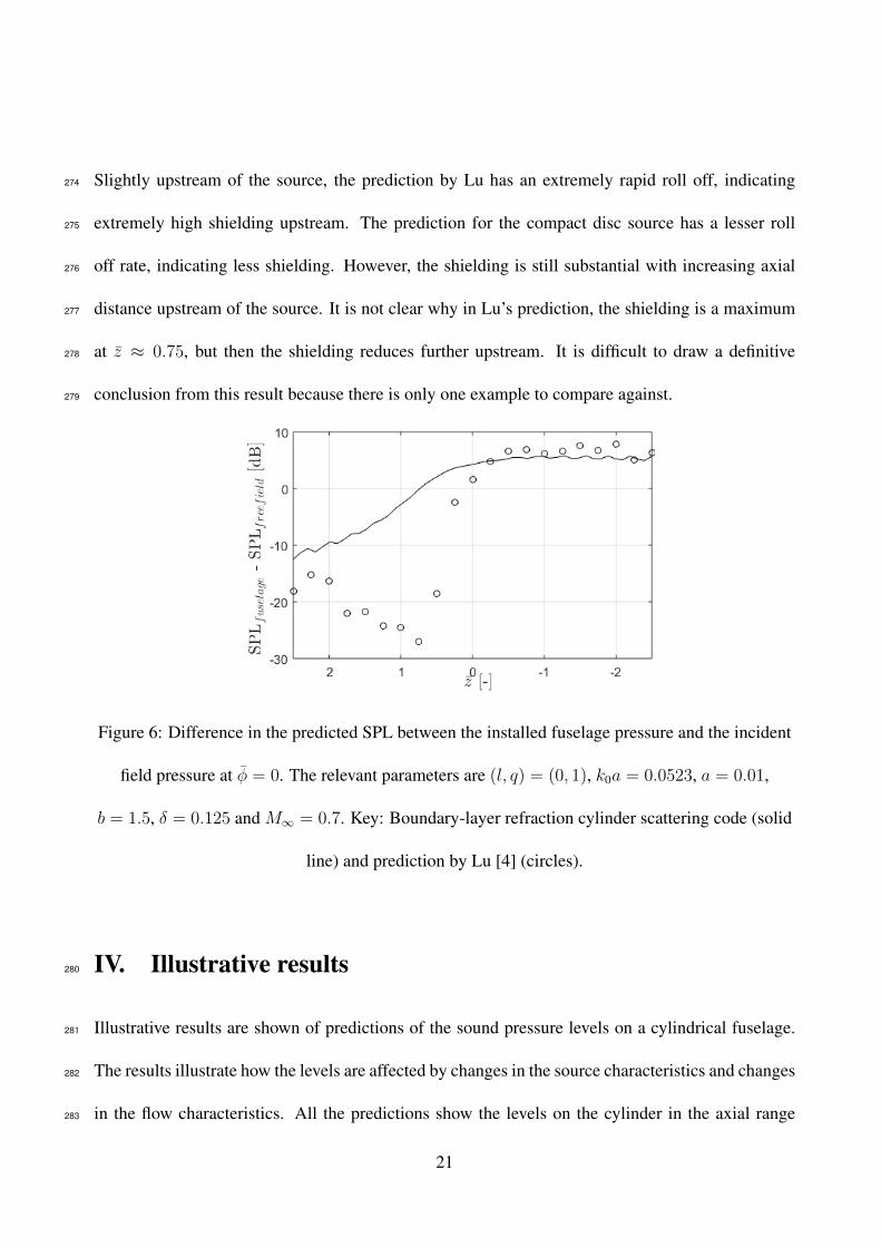
Slightly upstream of the source, the prediction by Lu has an extremely rapid roll off, indicating274

extremely high shielding upstream. The prediction for the compact disc source has a lesser roll275

off rate, indicating less shielding. However, the shielding is still substantial with increasing axial276

distance upstream of the source. It is not clear why in Lu’s prediction, the shielding is a maximum277

at z ≈ 0.75, but then the shielding reduces further upstream. It is difficult to draw a definitive278

conclusion from this result because there is only one example to compare against.279

Figure 6: Difference in the predicted SPL between the installed fuselage pressure and the incident

field pressure at φ = 0. The relevant parameters are (l, q) = (0, 1), k0a = 0.0523, a = 0.01,

b = 1.5, δ = 0.125 and M∞ = 0.7. Key: Boundary-layer refraction cylinder scattering code (solid

line) and prediction by Lu [4] (circles).

IV. Illustrative results280

Illustrative results are shown of predictions of the sound pressure levels on a cylindrical fuselage.281

The results illustrate how the levels are affected by changes in the source characteristics and changes282

in the flow characteristics. All the predictions show the levels on the cylinder in the axial range283

21

0 < z < 5, which roughly is comparable with the length of the fuselage forward of the engine, for284

airplanes with wing-mounted engines. For clarity, the results are shown for one source, on the right285

hand side of the fuselage, and for a single mode. Results are compared for a thin boundary-layer,286

δ = 0.01, or a relatively thick boundary-layer, δ = 0.1.287

Published values for the typical boundary-layer thickness on an aircraft fuselage are difficult288

to find. Recently some realistic predictions were in Ref.[14]. In this paper the maximum thickness289

(99%M∞) is around 0.1a0 in the plane of the engines. Flat plate predictions for a turbulent boundary290

layer thickness also predict a value for δ of around 0.1a0 at this plane.291

Two metrics are used to evaluate the effect of the boundary layer on the levels on the cylinder.292

First, we examine the difference in the predicted SPL on the cylinder with and without the boundary293

layer, i.e.294

∆ [dB] = SPLbl − SPL. (29)

The difference ∆ is useful for predicting the reduction in the ‘hot spot’ (region where the SPL on295

the cylinder is at a maximum). However, just examining the ∆’s can be misleading. For example, a296

large ∆ predicted on the far side of the cylinder will not be significant because it has been observed297

that with uniform flow, i.e. no boundary-layer shielding, the levels on the far side of the cylinder are298

low. A large reduction in these levels is not important to cabin noise.299

Next, to obtain a more overall view of the boundary-layer effect we introduce a simple ‘shielding’300

coefficient, denoted by S . The shielding coefficient is defined as the ratio of the area-averaged mean301

square pressure over the cylinder’s surface, with and without the boundary layer included in the302

prediction model. This value is, in turn, roughly proportional to the amount of the acoustic energy303

of the incident wave refracted away from the cylinder by the boundary layer. Accordingly, we define304

22

S by305

S =(1/A)

∫Ap2bl dA

(1/A)∫Ap2 dA

≈∑M p2

bl∑M p2, (30)

where in practice it is sufficient to evaluate S via a sum of the predicted mean square pressures over306

the M grid points distributed over the cylinder’s surface. The value of S will be between 0 and 1,307

where zero represents total shielding and unity represents no shielding.308

The results shown in Sections A.,B. examine predictions of S for three different boundary-layer309

profiles. These profiles are linear (δl), quarter-sine (δs) and a representative ‘turbulent’ seventh-310

power-law mean-flow profile (δt), where for each profile δ denotes the boundary-layer thickness. A311

quarter-sine velocity profile was chosen for the source parametric study in Sec. A.. This profile is312

reasonably similar to a Pohlausen profile which was used by Lu [4]. In Sec. B. predictions for the313

different boundary-layer profiles are compared. For reference, all the relevant profiles are plotted in314

Figure 7. For each profile, the location of the critical point can be found exactly. This location must315

be calculated numerically for more complicated profile shapes.316

A. Source characteristics317

In this section the source characteristics are changed whilst the boundary-layer flow profile and318

free-stream velocity are kept fixed. However, the effect of a thin or thick boundary-layer, having the319

same profile shape, is investigated.320

Figure 8(a–c) show examples of the results. Figure 8(a) shows the result with uniform flow,321

δ = 0.0. This case is used as a reference to compare with a thin boundary-layer δ = 0.01 shown322

in Figure 8(b), and a thick boundary-layer δ = 0.1 shown in Figure 8(c). Note that all results are323

normalised, so that the maximum SPL is equal to zero with uniform flow.324

23

Figure 7: Normalised boundary-layer profiles. Key: linear (solid line), 1/7th-power law (×),

quarter sine () and Polhausen (4).

The value of the source Helmholtz number k0a will determine the structure of the source’s polar325

directivity pattern. For the plane wave mode, at very low values of k0a, in this limit the source326

becomes omnidirectional. For non-plane-wave modes, the level at the intake duct’s axis will be327

zero. But whilst the frequency remains low, no side lobes are present. As the frequency increases,328

along with the principal lobe of radiation, more and more side lobes will be present. For a state-of-329

the-art turbofan engine, a typical k0a value of the blade passing frequency tone is around 20. In the330

examples in this section, the source Helmholtz numbers are taken to be k0a = 5, 10 and 20.331

Figure 9 plots the value of ∆ at φ = 0 for the three different source Helmholtz numbers. It is332

seen that for increasing frequency (k0a) the refraction effect of the boundary layer increases. In the333

plane of the source the shielding is a moderate 2-3 dB for a thin boundary-layer profile, however334

the shielding for a thick profile is 10 dB for the high frequency case. At high frequencies, refraction335

by the boundary layer can be more significant since the acoustic wavelength will be comparable or336

24

smaller compared to the boundary-layer thickness.337

Further upstream of the source plane, the shielding increases. More shielding is expected up-338

stream because the angle of incidence relative to the boundary layer decreases. Even for the lowest339

value of k0a for a thin boundary layer, at z = 5, the value of ∆ is around 18 dB. At shallow an-340

gles, the wave will be highly refracted by the shear layer. In general, shielding increases with both341

increasing frequency and boundary-layer thickness; also shielding increases as the grazing angle342

relative to the boundary layer becomes less.343

For k0a = 5, the polar directivity of the source has only one lobe. For the other cases, side344

lobes are present. The locations of nulls in the source’s polar directivity are slightly shifted by the345

boundary-layer; the effect of this can be seen in the levels on the surface of the cylinder, via dips in346

the plots of ∆.347

The ‘shielding’ coefficient S calculated for the three different source Helmholtz numbers are348

shown on Figure 9 next to the relevant line. At frequency k0a = 5, and for a thin boundary-layer,349

S = 0.37. In this case the area-averaged mean square pressure with the boundary layer is 63 % less350

than without the boundary layer included in the modelling. As a rough approximation, around two-351

thirds of the incident energy is refracted away from the cylinder’s surface by the boundary layer.352

With a thick boundary layer the reduction is close to 95 % (S = 0.056). As is seen in Figure 9,353

large reductions are present on the near side of the cylinder adjacent to the source. On the cylinder’s354

surface at r = a0, the shear for the quarter-sine profile is strongest. Thus as the waves creep around355

the cylinder, the wave is immersed in the boundary layer, and strong shielding occurs on the far side356

as well.357

Figure 10 shows the normalised SPL on the surface of the cylinder for mode (l, q) = (24, 1). The358

frequency k0a = 20 which means that this mode is only just cut on. The source directivity is such359

25

Figure 8: Normalised total SPL on the surface of the cylinder: (a) uniform flow, δ = 0.0; (b)

δ = 0.01; and, (c) δ = 0.1. The source is included in (c) for perspective. The relevant parameters

are (l, q) = (4, 1), k0a = 10, b = 3 and M∞ = 0.75.

26

Figure 9: Prediction of ∆ at φ = 0 for different values of the source Helmholtz number k0a. The

relevant parameters are (l, q) = (4, 1), a = 0.5, b = 3 and M∞ = 0.75. Key: Solid lines denote a

boundary layer of thickness δ = 0.01 and dashed lines are for δ = 0.1. The varying Helmholtz

numbers are k0a = 5 (no symbol), k0a = 10 (), and k0a = 20 (×).

27

δ

ka = 10 ka = 20

l l

4 4 24

0.01 0.1065 0.0590 0.2713

0.1 0.0055 0.0022 0.0119

Table 2: ‘Shielding’ coefficient S for the examples shown in Figures 8 and 10. In Figure 8, the

frequency k0a = 10 and the mode (l, q) = (4, 1). Note that the mode (l, q) = (24, 1) is cut-off at

this frequency. In Figure 10, the frequency k0a = 20 with the mode (l, q) = (24, 1). For

comparison, also the values of S for mode (l, q) = (4, 1) which are shown at this higher frequency.

that only a single lobe intersects with the cylinder at an axial position close to the source plane. On360

the near side of the cylinder, there is some increase in the shielding as the boundary-layer thickness361

is increased, but the overall effect is less comparing Figure 10 with the previous example shown in362

Figure 8. This is due to the angle of incidence of the mode; for a mode that is only just cut on, the363

angle will be close to 90 relative to the boundary layer. A wave impinging at a shallower angle is364

far more susceptible to the effects of the boundary layer. The values of the ‘shielding’ coefficient S365

calculated for the examples shown in Figures 8 and 10 are shown in Table 2.366

An alternative way to look at the effect of the boundary layer can be demonstrated by plotting367

an example of the function αn(kz), with and without the boundary layer, as shown in Figure 11.368

The function αn is largely unchanged for negative axial wavenumbers (waves travelling in the same369

direction as the flow), but the large fluctuations for positive axial wavenumbers are significantly370

reduced when the boundary layer is included in the calculation. In the Fourier domain the boundary371

28

Figure 10: Normalised total SPL on the surface of the cylinder: (a) uniform flow, δ = 0.0; (b)

δ = 0.01; and, (c) δ = 0.1. The relevant parameters are (l, q) = (24, 1), k0a = 20, a = 0.5, b = 3

and M∞ = 0.75

29

Figure 11: The function αn for the zeroth azimuthal mode. The relevant parameters are k0a = 10,

a = 0.5, b = 3 and M∞ = 0.75. Key: δ = 0 (solid line); δ = 0.1 (dashed line and squares).

layer acts as a low-pass filter.372

We note that although the polar directivity of the spinning mode source is axisymmetric, on the373

rigid cylinder the pressure patterns are slightly asymmetric. It can be shown that374

pt (l,−φ) = (−1)l pt (−l, φ) . (31)

Note the phase change for odd azimuthal orders.375

B. Flow characteristics376

In this section the flow characteristics are changed whilst the source is kept fixed. The source377

frequency is k0a = 20 and source mode is (l, q) = (16, 1). Results are compared for the linear,378

quarter-sine and 1/7th power law turbulent mean-flow boundary-layer profiles, as shown in Figure 7.379

The effect of varying the flow speed can be found in Gaffney, McAlpine and Kingan [15]380

Figure 12(a) shows a plot of the values of ∆ at φ = 0 for the three different boundary-layer381

30

Figure 12: Prediction of ∆ at φ = 0 for two different boundary-layer profiles: (a) δ fixed; (b) δ?

fixed. The relevant parameters are (l, q) = (16, 1), k0a = 20 , a = 0.5, b = 3 and M∞ = 0.75.

Key: thin boundary-layer (solid lines) or thick boundary-layer (dashed lines); boundary-layer

profiles, linear (×), quarter-sine (no symbol), 1/7th-power law ().

31

profiles. Results are shown for both the thin and thick boundary-layers. The shielding predicted for382

the linear and quarter-sine boundary-layer profiles are fairly similar. For this example, the mode is383

moderately cut-on, so moving further upstream, at z = 5 the levels on the cylinder are very low384

with or without the boundary layer included in the prediction scheme.385

The power law mean-flow profile is predicted to cause significantly less shielding along the cylin-386

der. The ‘shielding’ coefficient is much larger compared with the other profiles, which corresponds387

to relatively higher pressure amplitudes on the cylinder’s surface.388

The results in Figure 12(b) are for the same profiles as in (a), however the thickness of the389

boundary layer profiles have been modified so that the displacement thicknesses δ? of each profiles390

are identical. It is seen that, in this case, the shielding is very similar. Predictions for the linear and391

quarter-sine profiles are almost identical. Also, the difference between the power-law profile and392

the linear profile has reduced from 15 dB at z = 3 to around only 3 dB, for predictions with the393

profiles having the same value of δ?. These results suggest that the size of the displacement thickess394

is a more important factor vis-a-vis the boundary-layer profile shape.395

V. Conclusions396

A theoretical method has been developed which can be used to predict the acoustic pressure on397

a cylindrical fuselage due to a disc source located adjacent to the cylinder, including the effect398

of refraction by the fuselage boundary layer. The key new aspect of this work is the use of a399

disc source to represent sound radiation from a spinning mode exiting a cylindrical duct. Previous400

similar analysis of cylindrical fuselage boundary-layer refraction effects have employed a point401

source [4] or a propeller/open rotor source [2, 3, 12, 5]. The application of the current work is the402

32

prediction of the radiated pressure field on an aircraft’s fuselage, which is relevant for the assessment403

of cabin noise, from an installed turbofan aero-engine. This method can be used for single-mode404

calculations of the pressure on a cylindrical fuselage, with arbitrary boundary-layer profile and405

thickness. The model is a simple representation of a fan tone radiated from a turbofan intake duct.406

The methodology extends the solution given by McAlpine, Gaffney and Kingan [6] which omitted407

the fuselage boundary layer, and assumed uniform flow everywhere. Illustrative results have shown408

that the sound pressure levels on the surface of the cylinder, upstream of the source, are predicted409

to be greatly reduced for simulations which include the fuselage boundary layer, even for a thin410

boundary layer. The boundary-layer ‘shielding’ is seen to be most effective for well cut on modes.411

This is because the incident pressure grazes the boundary layer, and is more susceptible to refraction.412

In order to quantify the effect of the boundary layer, a ratio termed the ‘shielding’ coefficient has413

been introduced. This coefficient provides a measure of the total shielding, over the whole area of414

the cylinder. It is seen that with a thick boundary-layer profile, most of the acoustic energy will be415

shielded, and since the sound energy is refracted away from the cylinder’s surface, the levels on the416

cylindrical fuselage are predicted to be low compared to the levels which are predicted based on a417

uniform free-stream velocity.418

Future work will focus on replacing the disc source which is used to model a spinning mode419

exiting a cylindrical duct by a more sophisticated technique, employing the Wiener–Hopf solution420

to model sound radiation from a turbofan intake. This method will include diffraction and scattering421

effects caused by the duct termination, which have been omitted in the current method. Thus, as well422

as providing a more realistic model of sound radiated from an intake duct, also the refractive effects423

of the fuselage boundary layer will be examined, both upstream and downstream of the source.424

33

All data supporting this study are openly available from the University of Southampton repository425

at http://dx.doi.org/10.5258/SOTON/400423426

Acknowledgments427

The authors wish to acknowledge the continuing financial support provided by Rolls-Royce plc428

through the University Technology Centre in Gas Turbine Noise at the Institute of Sound and Vi-429

bration Research. The first author also acknowledges the financial contribution from the EPSRC via430

the University of Southampton’s DTP grant.431

34

References432

[1] J. Bowman, T. Senior, and P. Uslenghi, eds., Electromagnetic and Acoustic Scattering by Sim-433

ple Shapes (Horth-Holland Publishing Co., Amsterdam) (1969).434

[2] D. Hanson, “Shielding of prop-fan cabin noise by the fuselage boundary layer”, Journal of435

Sound and Vibration 22, 63–70 (1984).436

[3] D. Hanson and B. Magliozzi, “Propagation of propeller tone noise through a fuselage boundary437

layer”, Journal of Aircraft 22, 63–70 (1985).438

[4] H. Lu, “Fuselage boundary-layer effects on sound propagation and scattering”, American In-439

stitute of Aeronautics and Astronautics Journal 28, 1180–1186 (1990).440

[5] H. Brouwer, “The scattering of open rotor tones by a cylindrical fuselage and its boundary441

layer”, Proceedings of the 22nd AIAA/CEAS Aeroacoustics conference, Lyon, France, AIAA442

paper no. 2016-2741 16 pp. (30 May–1 June, 2016).443

[6] A. McAlpine, J. Gaffney, and M. Kingan, “Near-field sound radiation of fan tones from an444

installed turbofan aero-engine”, Journal of the Acoustical Society of America 138, 131–1324445

(2015).446

[7] J. Tyler and T. Sofrin, “Axial flow compressor noise studies”, SAE Transactions 70, 309–332447

(1962).448

[8] S. Hocter, “Exact and approximate directivity patterns of the sound radiated from a cylindrical449

duct”, Journal of Sound and Vibration 227, 397–407 (1999).450

35

[9] E. Rice, M. Heidmann, and T. Sofrin, “Modal propagation angles in a cylindrical duct with451

flow and their relation to sound radiation”, 17th Aerospace Sciences Meeting, New Orleans,452

LA, AIAA paper no. 79-0183 (15–17 January, 1979).453

[10] E. Brambley, M. Darau, and S. Rienstra, “The critical layer in linear-shear boundary layers454

over acoustic linings”, Journal of Fluid Mechanics 710, 545–568 (2012).455

[11] In fact this is the opposite branch to that selected in Ref. [3], because in this current work the456

time-dependence is exp iωt, whereas in Ref.[3] the authors used exp −iωt.457

[12] I. Belyaev, “The effect of an aircraft’s boundary layer on propeller noise”, Acoustical Physics458

58, 425–433 (2012).459

[13] This assumes that the boundary-layer mean flow profile does not allow solutions of the460

Pridmore-Brown equation which are exponentially small at r = 1.461

[14] A. Klabes, C. Appel, M. Herr, and M. Bouhaj, “Fuselage excitation during cruise flight462

conditions: measurement and prediction of pressure point spectra”, Proceedings of the 21st463

AIAA/CEAS Aeroacoustics conference, Dallas, TX, AIAA paper no. 2015-3115 23 pp. (22–464

26 June, 2015).465

[15] J. Gaffney, A. McAlpine, and M. Kingan, “Sound radiation of fan tones from an installed466

turbofan aero-engine: fuselage boundary-layer refraction effects”, Proceedings of the 22nd467

AIAA/CEAS Aeroacoustics conference, Lyon, France, AIAA paper no. 2016-2878 23 pp. (30468

May–1 June, 2016).469

36

List of Figures470

1 Sketch of the cylindrical fuselage (radius a0) and the disc source (radius a). The471

centreline of the cylinder is aligned with the z-axis. The disc source is located in472

the plane z = 0, and the distance between the centre of the disc and the centre of473

the cylinder is b. Also shown is the edge of the fuselage boundary-layer (thickness δ). 6474

2 Normalised total SPL on the surface of the cylinder. The location of the maximum475

value of the SPL is shown by the blue dot. Predictions of this point obtained using476

(i) mode (phase) angle, (ii) radiation angle (11), or (iii) numerical evaluation of477

the near-field (in the absence of the cylinder), are also shown. Key: (i) magenta478

dot; (ii) black dot; (iii) green dot. Other relevant parameters in this example are479

(l, q) = (2, 1), k0a = 5, b = 3 and M∞ = 0.5. . . . . . . . . . . . . . . . . . . . . 10480

3 Illustration showing the method to solve the Pridmore-Brown equation in the bound-481

ary layer. The numerical solution obtained using a standard ODE solver, for har-482

monic n, is matched to the Frobenius solution either side of the critical layer, in483

order to bridge the critical point rc. . . . . . . . . . . . . . . . . . . . . . . . . . . 15484

4 Comparison of the boundary-layer refraction and uniform flow cylinder scattering485

codes: (a) SPL; (b) relative error, δ = 0.01; (c) relative error, δ = 0.1. The relevant486

parameters in this example are (l, q) = (16, 1), k0a = 20, a = 0.6, b = 6 and487

M∞ = 0.7. . . . . . . . . . . . . . . . . . . . . . . . . . . . . . . . . . . . . . . 18488

37

5 Effect of width of the critical layer (Frobenius solution) andnumber of interpola-489

tion points used to evaluate I1: (a) absolute error; (b) relative error. The relevant490

parameters in this example are (l, q) = (0, 1), k0a = 0.0524, a = 0.01, b = 1.5,491

δ = 0.125 and M∞ = 0.7. Key: ε = 0.0002 (orange dashes), 0.001 (yellow dots),492

0.002 (purple dash dots), 0.003 (green ), 0.005 (cyan ∇) and 0.01 (maroon4). . . 19493

6 Difference in the predicted SPL between the installed fuselage pressure and the494

incident field pressure at φ = 0. The relevant parameters are (l, q) = (0, 1), k0a =495

0.0523, a = 0.01, b = 1.5, δ = 0.125 and M∞ = 0.7. Key: Boundary-layer496

refraction cylinder scattering code (solid line) and prediction by Lu [4] (circles). . . 21497

7 Normalised boundary-layer profiles. Key: linear (solid line), 1/7th-power law (×),498

quarter sine () and Polhausen (4). . . . . . . . . . . . . . . . . . . . . . . . . . 24499

8 Normalised total SPL on the surface of the cylinder: (a) uniform flow, δ = 0.0;500

(b) δ = 0.01; and, (c) δ = 0.1. The source is included in (c) for perspective. The501

relevant parameters are (l, q) = (4, 1), k0a = 10, b = 3 and M∞ = 0.75. . . . . . . 26502

9 Prediction of ∆ at φ = 0 for different values of the source Helmholtz number k0a.503

The relevant parameters are (l, q) = (4, 1), a = 0.5, b = 3 and M∞ = 0.75. Key:504

Solid lines denote a boundary layer of thickness δ = 0.01 and dashed lines are for505

δ = 0.1. The varying Helmholtz numbers are k0a = 5 (no symbol), k0a = 10 (),506

and k0a = 20 (×). . . . . . . . . . . . . . . . . . . . . . . . . . . . . . . . . . . . 27507

10 Normalised total SPL on the surface of the cylinder: (a) uniform flow, δ = 0.0; (b)508

δ = 0.01; and, (c) δ = 0.1. The relevant parameters are (l, q) = (24, 1), k0a = 20,509

a = 0.5, b = 3 and M∞ = 0.75 . . . . . . . . . . . . . . . . . . . . . . . . . . . . 29510

38

11 The function αn for the zeroth azimuthal mode. The relevant parameters are k0a =511

10, a = 0.5, b = 3 and M∞ = 0.75. Key: δ = 0 (solid line); δ = 0.1 (dashed line512

and squares). . . . . . . . . . . . . . . . . . . . . . . . . . . . . . . . . . . . . . 30513

12 Prediction of ∆ at φ = 0 for two different boundary-layer profiles: (a) δ fixed; (b)514

δ? fixed. The relevant parameters are (l, q) = (16, 1), k0a = 20 , a = 0.5, b = 3 and515

M∞ = 0.75. Key: thin boundary-layer (solid lines) or thick boundary-layer (dashed516

lines); boundary-layer profiles, linear (×), quarter-sine (no symbol), 1/7th-power517

law (). . . . . . . . . . . . . . . . . . . . . . . . . . . . . . . . . . . . . . . . . 31518

39