Gildenblatt, Robbie 12-17-12

A Methodology Incorporating Manufacturing System Capacity in Manufacturing Cost

Estimation

A thesis presented to

the faculty of

the Russ College of Engineering and Technology of Ohio University

In partial fulfillment

of the requirements for the degree

Master of Science

Robbie B. Gildenblatt

December 2012

© 2012 Robbie B. Gildenblatt. All Rights Reserved.

2

This thesis titled


Estimation

by

ROBBIE B. GILDENBLATT

has been approved for

the Department of Industrial and Systems Engineering

and the Russ College of Engineering and Technology by

Dale T. Masel

Associate Professor

Dennis Irwin

Dean, Russ College of Engineering and Technology

3

ABSTRACT

GILDENBLATT, ROBBIE B., M.S., December 2012, Industrial and Systems

Engineering


Estimation

Director of Thesis: Dale T. Masel

Using Design for Manufacturability to integrate manufacturing and design has

been shown over the years to reduce manufacturing costs and increasing overall

revenues. Much research has been provided with a focus on integrating the design of a

product and its respective manufacturing processes, but without the consideration of the

existing facility capacity. By incorporating the existing capacity, manufacturing cost

estimations can more accurately represent true factors such as overtime and material

handling.

This thesis describes a methodology to incorporate system capacity in cost

estimation. Ideal manufacturing costs, widely used as a standard for production cost

estimation, incorporates only material and labor costs. Ideal cost is used as an input to

the methodology proposed, and determines true manufacturing costs using the existing

manufacturing system design.

The methodology compares multiple possible designs for a given part and

estimates true cost of each design. Along with estimating true cost, the methodology

considers three alternatives for implementing each design and the total costs of each:

minimizing material handling costs by minimizing intracellular movement; minimizing

4

overtime costs by utilizing all machine capacity, and minimizing total costs by

purchasing additional machines to meet demand.

The methodology will provide an estimate of the true cost for each design being

evaluated for each alternative presented. This will allow the user to not only get a more

accurate representation of manufacturing costs, but also allow for cost analysis of

multiple implementation alternatives for versatility. A mathematical model which

maximizes facility profit by using the methodology proposed will be created and

evaluated. The model will show how the methodology presented can be used in

alternative scenarios in manufacturing settings.

5

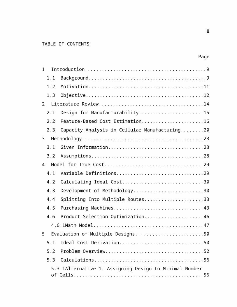
TABLE OF CONTENTS

Page

1 Introduction..................................................................................................................9

1.1 Background..........................................................................................................9

1.2 Motivation..........................................................................................................11

1.3 Objective............................................................................................................12

2 Literature Review......................................................................................................14

2.1 Design for Manufacturability............................................................................15

2.2 Feature-Based Cost Estimation..........................................................................16

2.3 Capacity Analysis in Cellular Manufacturing...................................................20

3 Methodology..............................................................................................................23

3.1 Given Information.............................................................................................23

3.2 Assumptions......................................................................................................28

4 Model for True Cost..................................................................................................29

4.1 Variable Definitions...........................................................................................29

4.2 Calculating Ideal Cost........................................................................................30

4.3 Development of Methodology...........................................................................30

4.4 Splitting Into Multiple Routes...........................................................................33

4.5 Purchasing Machines.........................................................................................43

4.6 Product Selection Optimization.........................................................................46

4.6.1 Math Model...................................................................................................47

5 Evaluation of Multiple Designs.................................................................................50

5.1 Ideal Cost Derivation.........................................................................................50

5.2 Problem Overview.............................................................................................52

5.3 Calculations.......................................................................................................56

5.3.1 Alternative 1: Assigning Design to Minimal Number of Cells.....................56

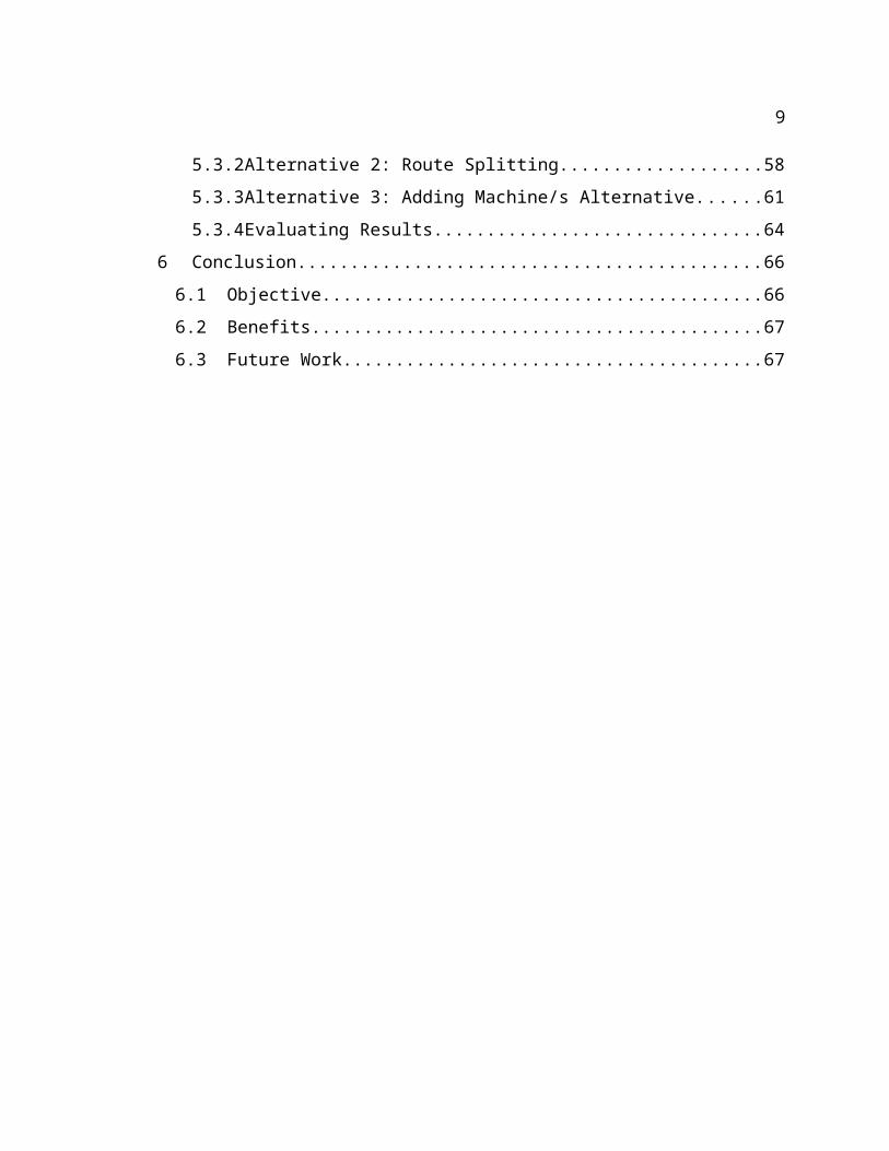
5.3.2 Alternative 2: Route Splitting........................................................................58

5.3.3 Alternative 3: Adding Machine/s Alternative................................................61

5.3.4 Evaluating Results.........................................................................................64

6 Conclusion.................................................................................................................66

6

6.1 Objective............................................................................................................66

6.2 Benefits..............................................................................................................67

6.3 Future Work.......................................................................................................67

7

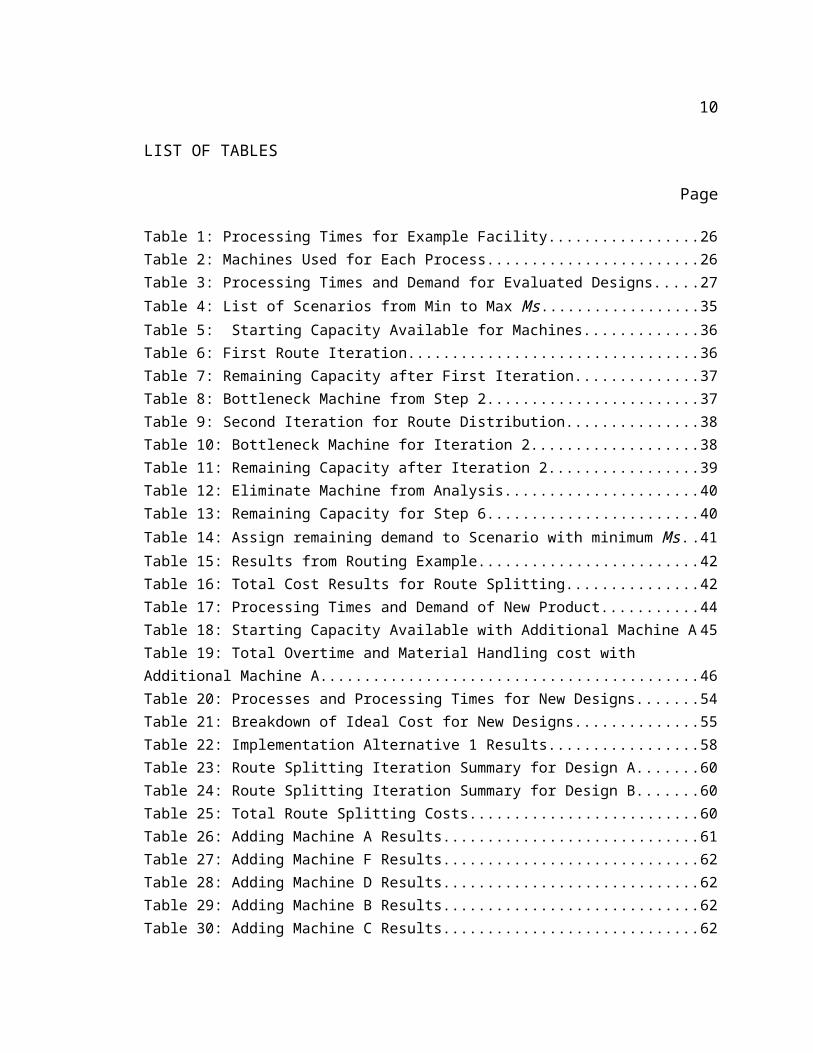
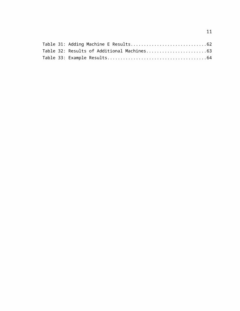
LIST OF TABLES

Page

Table 1: Processing Times for Example Facility.............................................................................26Table 2: Machines Used for Each Process.....................................................................................26Table 3: Processing Times and Demand for Evaluated Designs....................................................27Table 4: List of Scenarios from Min to Max Ms............................................................................35Table 5: Starting Capacity Available for Machines.......................................................................36Table 6: First Route Iteration........................................................................................................36Table 7: Remaining Capacity after First Iteration..........................................................................37Table 8: Bottleneck Machine from Step 2.....................................................................................37Table 9: Second Iteration for Route Distribution..........................................................................38Table 10: Bottleneck Machine for Iteration 2...............................................................................38Table 11: Remaining Capacity after Iteration 2.............................................................................39Table 12: Eliminate Machine from Analysis..................................................................................40Table 13: Remaining Capacity for Step 6......................................................................................40Table 14: Assign remaining demand to Scenario with minimum Ms...........................................41Table 15: Results from Routing Example......................................................................................42Table 16: Total Cost Results for Route Splitting............................................................................42Table 17: Processing Times and Demand of New Product............................................................44Table 18: Starting Capacity Available with Additional Machine A.................................................45Table 19: Total Overtime and Material Handling cost with Additional Machine A.......................46Table 20: Processes and Processing Times for New Designs.........................................................54Table 21: Breakdown of Ideal Cost for New Designs....................................................................55Table 22: Implementation Alternative 1 Results...........................................................................58Table 23: Route Splitting Iteration Summary for Design A............................................................60Table 24: Route Splitting Iteration Summary for Design B............................................................60Table 25: Total Route Splitting Costs............................................................................................60Table 26: Adding Machine A Results.............................................................................................61Table 27: Adding Machine F Results.............................................................................................62Table 28: Adding Machine D Results............................................................................................62Table 29: Adding Machine B Results.............................................................................................62Table 30: Adding Machine C Results.............................................................................................62Table 31: Adding Machine E Results.............................................................................................62Table 32: Results of Additional Machines.....................................................................................63Table 33: Example Results............................................................................................................64

8

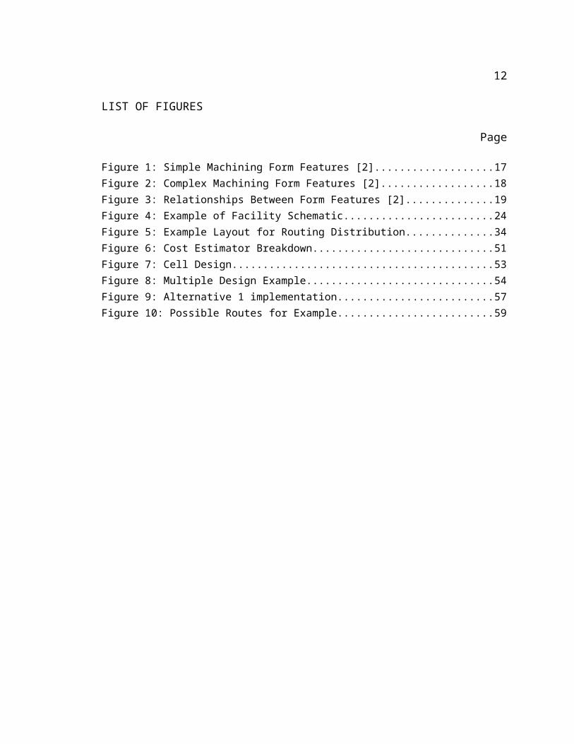
LIST OF FIGURES

Page

Figure 1: Simple Machining Form Features [2].............................................................................17Figure 2: Complex Machining Form Features [2]..........................................................................18Figure 3: Relationships Between Form Features [2].....................................................................19Figure 4: Example of Facility Schematic........................................................................................24Figure 5: Example Layout for Routing Distribution.......................................................................34Figure 6: Cost Estimator Breakdown.............................................................................................51Figure 7: Cell Design.....................................................................................................................53Figure 8: Multiple Design Example...............................................................................................54Figure 9: Alternative 1 implementation........................................................................................57Figure 10: Possible Routes for Example........................................................................................59

9

1 Introduction

There is a gap in Industry between design and manufacturing departments, which

can lead to poor decisions made in product development. Due to this gap, decisions

made in the design phase of product development may not have input from

manufacturing departments, potentially leading to problems in manufacturing, resulting

in increased manufacturing costs and overall waste. This gap is caused by a lack of

communication between design and manufacturing departments.

1.1 Background

Concurrent engineering, or Design for Manufacturability (DFM), is a work

practice which proposes to reduce the communication gap between these two

departments. DFM is aimed at maintaining a product’s performance while reducing its

lead time, total cost, and improving the quality of a design with less redesigns [5].

Eliminating the communication gap between these two departments can reduce overall

cost of production.

Products are initially designed to meet identified performance objectives and

specifications while providing a specific capability. DFM is usually concerned with

minimizing the costs of traditional operating aspects such as function, reliability, safety,

marketability, ergonomics, and aesthetics. What many companies overlook is the

importance of the product’s manufacturability and how it can be designed to eliminate

unnecessary manufacturing costs.

Manufacturability is the degree to which a product can be manufactured. This

includes how easy or difficult a product is to manufacture and at what cost [12]. Unlike

10

traditional product design, which focuses on operating aspects of a product,

manufacturability is concerned with non-operating aspects of a product such as material

handling costs, overtime costs, machine procurement, and overall ease of production.

Manufacturing is concerned with all operations necessary to produce a given product.

Every new product that is introduced into an industry has to be producible, and

there are degrees of difficulty regarding each product to be produced. The more difficult

a product is to produce, the more expensive the product will be to produce. The goal of

many manufacturing companies is to maximize manufacturability, which in turn reduces

overall manufacturing costs and increases production rates. Production rate, from a

manufacturing standpoint, is the measure of units produced in a given time frame. This

measure can provide detailed information about the output of manufacturing processes

and is essential to maximize when designing and operating a facility.

DFM eliminates many manufacturing problems during the design phase, which is

the most cost effective place to address these problems. Research has shown that 70% of

a product’s cost is determined by decisions made during the design period, while

decisions made during production only account for 20% of the product’s costs [18].

DFM is a key tool in minimizing those costs and providing higher profits.

DFM considers the manufacturability of a product within the preliminary design

stage. DFM incorporates the analysis of manufacturing costs and expenses in the

preliminary design phase and attempts to minimize them before manufacturing has even

begun. Many companies lack DFM in their design phase, resulting in manufacturing

11

problems down the road. This ultimately results in excess costs and time wasted on

problems which could be avoided using DFM in early stages of product development.

1.2 Motivation

Traditionally, manufacturability refers to only labor and material costs. Previous

research has shown that by determining how much time and material a product would

take to manufacture, material costs and labor cost were estimated, which would account

for manufacturing costs. As more research has been provided, more variables are

accounted for in manufacturability such as tool changes, material handling costs, adding

machines, overtime, and many others.

Feature-based cost estimators play an important role in analyzing

manufacturability. A feature-based cost estimator is a program which represents a

product by using key feature dimensions and connecting these defined features to create a

geometric representation of the product. The feature-based cost estimator allows the cost

of processes such as milling, drilling, and turning to be estimated for the given features.

The program defines each feature with dimensions such as height, length, outer diameter,

inner diameter, thickness, and other key geometrically-influential parameters. Once all

features are modeled correctly and the product is defined as a whole, the cost estimator

outputs labor hours and costs for the appropriate manufacturing processes. The outputs

of estimated labor hours and costs provide insight into the manufacturability.

The output of a feature-based cost estimator represents the ideal manufacturing

cost of a product. The ideal manufacturing cost includes only material costs and labor

costs without consideration of labor costs fluctuating depending on overtime. The ideal

12

labor cost simply sums the manufacturing time and multiplies it by the labor rate.

Employees, however, receive an increased hourly rate when working overtime.

This thesis, however, is interested in true cost. The true cost of manufacturing

goes beyond labor to include such factors as capacity, machine availability, operator

availability, machine procurement, and material handling. As capacity used in a facility

increases, overtime may need to be used to meet demand or purchasing new equipment to

save overtime costs. The knowledge of machine capacity and availability is critical in

determining how much time is available to manufacture within working hours, and how

much time will be needed for overtime. Material handling, which is not considered in

ideal cost, can provide significant additional manufacturing costs depending on distances

materials must travel. Material handling creates additional labor time, which translates to

extra labor cost needed to pay workers.

The ideal manufacturing process times and material cost from a feature-based cost

estimator can then create a source of inputs to the methodology proposed, providing a

foundation for calculations of true manufacturing costs of a given design.

1.3 Objective

The objective of this thesis is to create a methodology which incorporates not

only traditional ideal costs, but also material handling and overtime costs to more

accurately represent manufacturability of preliminary product designs. By incorporating

system capacity data into manufacturing cost calculations, overtime costs, machine

procurement costs, and material handling costs can be determined in addition to ideal

costs calculated from the feature-based cost estimator. This will provide an estimate of

13

the true manufacturing cost when adding a given product design to the facility, enabling a

more accurate manufacturing cost to design selection as well as mulitple implementation

options.

14

2 LITERATURE REVIEW

This literature review is composed of three separate sections—Design for

Manufacturability, Feature-based Cost Estimation, and Capacity Analysis, all of which

provide the foundation for this research and proposed methodology.

The feature-based cost estimator will geometrically represent a given product

using a computer program, which can allow a user to input geometric dimensions to

estimate the product’s material and labor costs. Once the material and labor costs are

estimated using the cost estimator, capacity analysis must be evaluated to accurately

select a cost effective product design based on the actual manufacturing system design.

The theory of DFM was used in this thesis to incorporate focus on intercellular

movement costs, and overtime costs. The methodology incorporates these factors for

implementation of a given product design into an already existing facility with

predesigned cells. Based on the existing manufacturing cells, the cost of each design will

be evaluated via the methodology proposed and offer three alternative implementation

methods to allow the user to evaluate costs of each.

It was important to research previous capacity analysis, specifically research in

which any of the cost factors used in this methodology were mentioned. This will allow

a better understanding of previous capacity analysis evaluation and how the methodology

proposed extends capacity analysis into a new direction—to minimize manufacturing

costs when implementing a new product based on its design in an already existing

cellular manufacturing environment. These three areas of topic provide a solid

foundation for previous research in the field.

15

2.1 Design for Manufacturability

It is important to understand previous research on DFM, specifically with regard

to manufacturing cost estimation. DFM can have a significant effect on the reduction of

manufacturing costs and provides a solid foundation for cost reductions in product

design.

Dowlatshahi [17] presents several advantages of DFM and its implementation.

He classifies the advantages into two categories: reduction in product development lead

time and overall cost savings. Reducing the number of redesigns in a system and the

amount of effort needed, DFM can potentially reduce product design cycle time. The

concept of DFM is designed to increase the flow of communication between decision

makers, ultimately increasing productivity and increasing efficiency in operations. The

cost savings are identified by several examples Dowlatashahi provides, as different

features both providing the same operational value to the part show varying

manufacturing costs. By evaluating these manufacturing costs prior to production,

Dowlatashahi proposes overall cost savings based on these decisions.

There have been many software systems and tools designed to implement DFM.

These systems have been developed using various types of analysis methods such as

numerical computation, knowledge engineering, fuzzy mathematics, neural networks, and

object oriented programming [11]. According to Xue and Dong [5], developing cost-

effective designs using DFM should have the following capabilities: providing design

requirements of a product; producing possible design alternatives; representing design

geometry; determining the production costs of each design; and identifying the cost-

16

effective design. The methodology presented in this thesis follows the capabilities

mentioned by Xue and Dong. In order to represent design geometry, a feature-based cost

estimator is used in this thesis.

2.2 Feature-Based Cost Estimation

In order to quantify labor and material costs of a part, part geometry can be

defined in a feature-based cost estimator. This paper uses a feature-based modeling

program to provide material costs and labor costs due to machining and other processes.

Features on a part can be categorized into classes, with each class presenting their own

properties and methodologies, simplifying the extent to which a feature can be

represented [2].

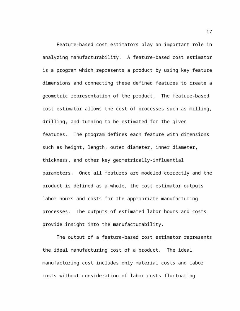
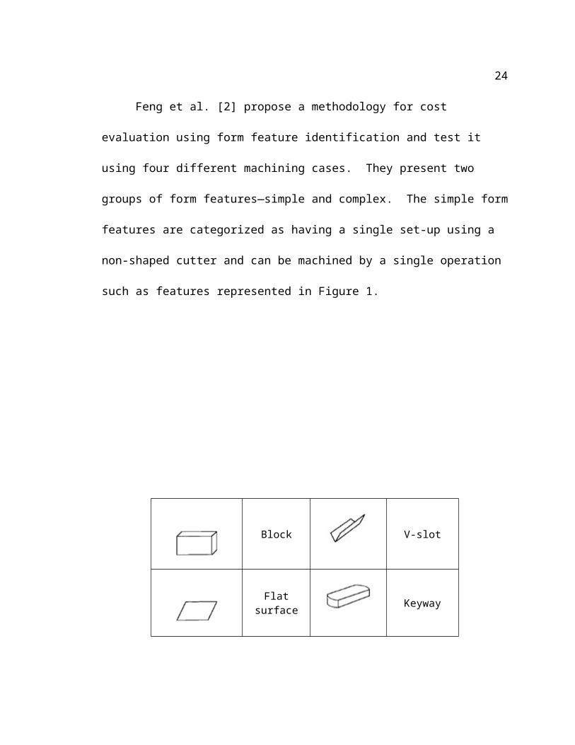
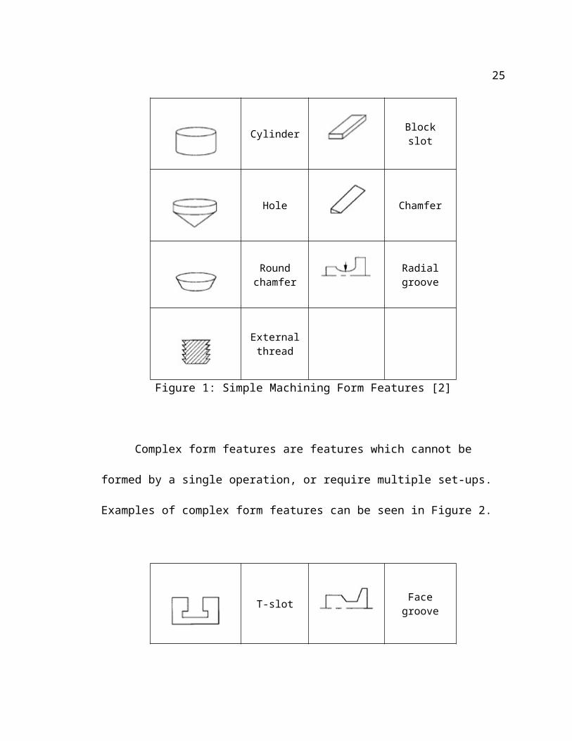
Feng et al. [2] propose a methodology for cost evaluation using form feature

identification and test it using four different machining cases. They present two groups

of form features—simple and complex. The simple form features are categorized as

having a single set-up using a non-shaped cutter and can be machined by a single

operation such as features represented in Figure 1.

17

Block V-slot

Flat surface Keyway

Cylinder Block slot

Hole Chamfer

Round chamfer Radial groove

External thread

Figure 1: Simple Machining Form Features [2]

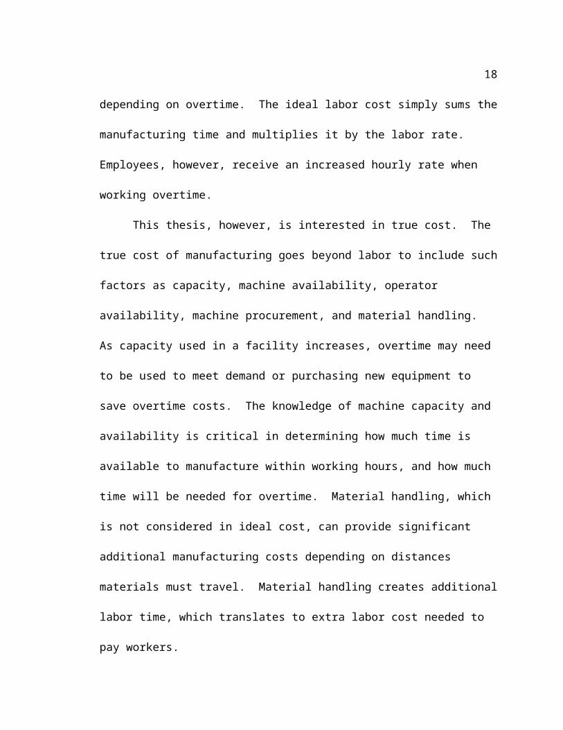
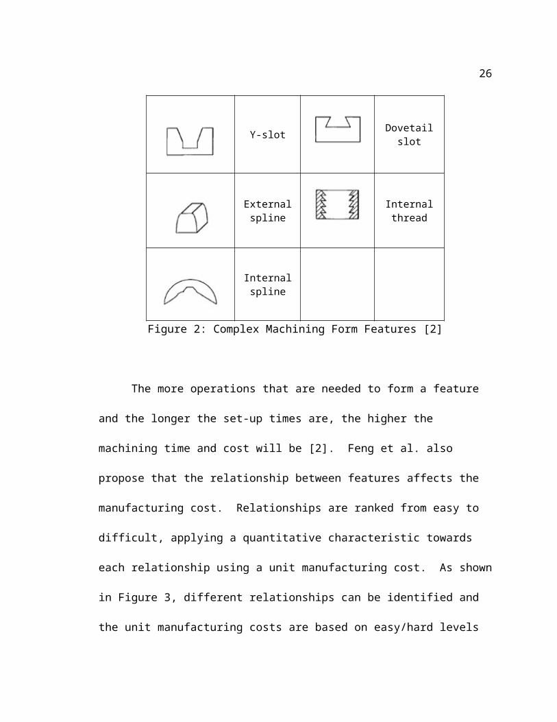
Complex form features are features which cannot be formed by a single operation,

or require multiple set-ups. Examples of complex form features can be seen in Figure 2.

18

T-slot Face groove

Y-slot Dovetail slot

External spline

Internal thread

Internal spline

Figure 2: Complex Machining Form Features [2]

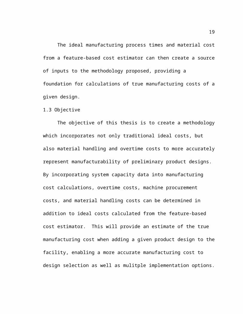
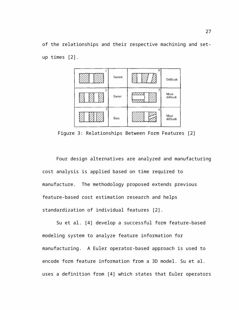
The more operations that are needed to form a feature and the longer the set-up

times are, the higher the machining time and cost will be [2]. Feng et al. also propose

that the relationship between features affects the manufacturing cost. Relationships are

ranked from easy to difficult, applying a quantitative characteristic towards each

relationship using a unit manufacturing cost. As shown in Figure 3, different

relationships can be identified and the unit manufacturing costs are based on easy/hard

levels of the relationships and their respective machining and set-up times [2].

19

Figure 3: Relationships Between Form Features [2]

Four design alternatives are analyzed and manufacturing cost analysis is applied

based on time required to manufacture. The methodology proposed extends previous

feature-based cost estimation research and helps standardization of individual features

[2].

Su et al. [4] develop a successful form feature-based modeling system to analyze

feature information for manufacturing. A Euler operator-based approach is used to

encode form feature information from a 3D model. Su et al. uses a definition from [4]

which states that Euler operators have been developed to aid in the generation of a solid’s

topology. Euler operators will add or delete attributes based on Euler’s formula for solid

objects.

According to Su et al. [4], previous attempts to provide shape knowledge of a part

have mostly been concentrated on feature recognition from solid models, group

technology coding schemes, and feature-based modeling. The problem with solid models

is that many CAD systems cannot provide lower-level geometric identities needed to

accurately define machining features. Due to this, most form feature programs, including

20

the one used in this paper, are separate from the solid modeling program used to design

the part.

2.3 Capacity Analysis in Cellular Manufacturing

There has been a lot of research done on capacity analysis ranging from

minimizing intercellular costs to minimizing cellular reconfiguration costs. The main

focus of previous research minimizes total cost, whether that cost includes overtime costs

or tool consumption costs.

Choi and Cho [9] propose a cost-based algorithm which uses production costs,

fixed machine costs, set-up costs, and material handling costs to assign parts and

machines to manufacturing cells based on the minimum cost. The algorithm considers

three separate alternatives when considering design of the system: the first alternative

tries to minimize the maximum number of intercellular movements; the second

alternative considers overtime as an option; the third alternative considers the possibility

of subcontracting the processing to outside vendors. The total cost for each alternative is

computed and the alternative with the minimum cost is chosen as the ideal design.

Choi and Cho’s research is very similar to this paper with regard to considering

alternatives such as minimizing intercellular movement and overtime; however, Choi and

Cho present a model which clusters parts and machines, identifies “exceptional” parts

which do not fit in only one cell, and provide cost analysis alternatives on only those

parts [9] while this thesis uses a pre-existing layout with pre-clustered cells for capacity

requirements. This thesis presents a more practical approach to adding a product to a pre-

21

existing facility by using the existing clustering of cells rather than re-clustering the cells,

which could result in excess downtime to redesign.

Defersha and Chen [6] propose a part-machine grouping methodology for the

design of cellular manufacturing systems based on multiple costs. Their objective is to

minimize machine maintenance and overhead costs, machine procurement costs, inter-

cellular movement costs, machine operation and setup costs, tool consumption costs, and

system reconfiguration costs.

For this method, a math model is presented and the cellular design was

determined based on minimum total cost. The intercellular cost in this problem uses a

fixed cost for material handling from one cell to another for independent parts. Batch

size and demand for each part are also used to determine the total number of trips for

each given part. The cost of adding and removing a machine from a cell is also used for

“reconfiguration costs,” by using a fixed cost for the addition and subtraction of a

machine independently. However, they only consider these costs for existing parts and

did not adapt the model for use in evaluating the cost of new products being designed as

this thesis will propose.

Mahdavi et al. [7] propose a math model for cellular manufacturing systems with

worker assignment for multiple time periods. The model’s objective is to minimize total

costs of intercellular material handling, holding and backorder costs, machine and

reconfiguration, hiring, firing, and salary worker costs. According to Mahdavi et al.,

system reconfiguration involves adding and removing machines along with the addition

and removal of workers from one cell to another. This thesis does not consider system

22

reconfiguration as an alternative to minimize cost. System reconfiguration is an

unnecessary alternative when introducing a single product to an existing facility. This

thesis focuses on product integration without the difficulty of system reconfiguration.

Ahkioon et al. presents a model with a focus on routing flexibility by formulating

alternate contingency process routings [16]. Contingency routings are used as a backup

in case a machine breaks down or there is a setback in a product original route. Ahkioon

et al. look at the manufacturing problem at an operational point of view, however, this

thesis focuses on hours available as a fixed variable. As a fixed value, hours available

will account for possible breakdowns and will not be considered as a separate variable.

The model presented by Ahkioon et al. does present an optimal cellular layout

model with an objective of minimizing costs of many manufacturing factors such as

machine maintenance, machine operation, outsourcing, inventory holding, production

costs, intercellular and intracellular material handling costs, and machine procurement

cost. These factors allow for an optimal cell configuration in terms of types of number of

machines assigned to a cell.

23

3 METHODOLOGY

This section will cover the methodology developed in this research to estimate

true manufacturing costs. Due to the complexity of this problem, certain assumptions

were made. This section will cover the problem at hand, discuss what data is known,

cover the assumptions that were made, discuss the methods for calculating true cost, and

visit the three implementation alternatives that the methodology consists of.

The problem that this method will address is to determine the true manufacturing

cost of different product designs. The true cost will incorporate not only ideal cost (labor

and material costs), but also material handling, overtime costs, and machine procurement

costs. The methodology will evaluate each design separately to determine manufacturing

costs for each design as well as evaluate each implementation option separately to give

the user multiple implementation alternatives.

The three implementation alternatives—minimizing material handling costs,

minimizing overtime costs by route splitting, and purchasing new machines to reduce

overtime—will allow for the user to evaluate different implementation options for each

design. This will allow for a preliminary estimate of true manufacturing costs for

different implementation processes, which can provide a great benefit to design

evaluation and implementation.

3.1 Given Information

The first given information needed is a cell design with its defined cells.

Information needed for cells will be machine types and machine quantities identified.

Each machines available capacity is also needed for the foundation of calculating

24

capacity available for each process, and determining all possible routing options for a

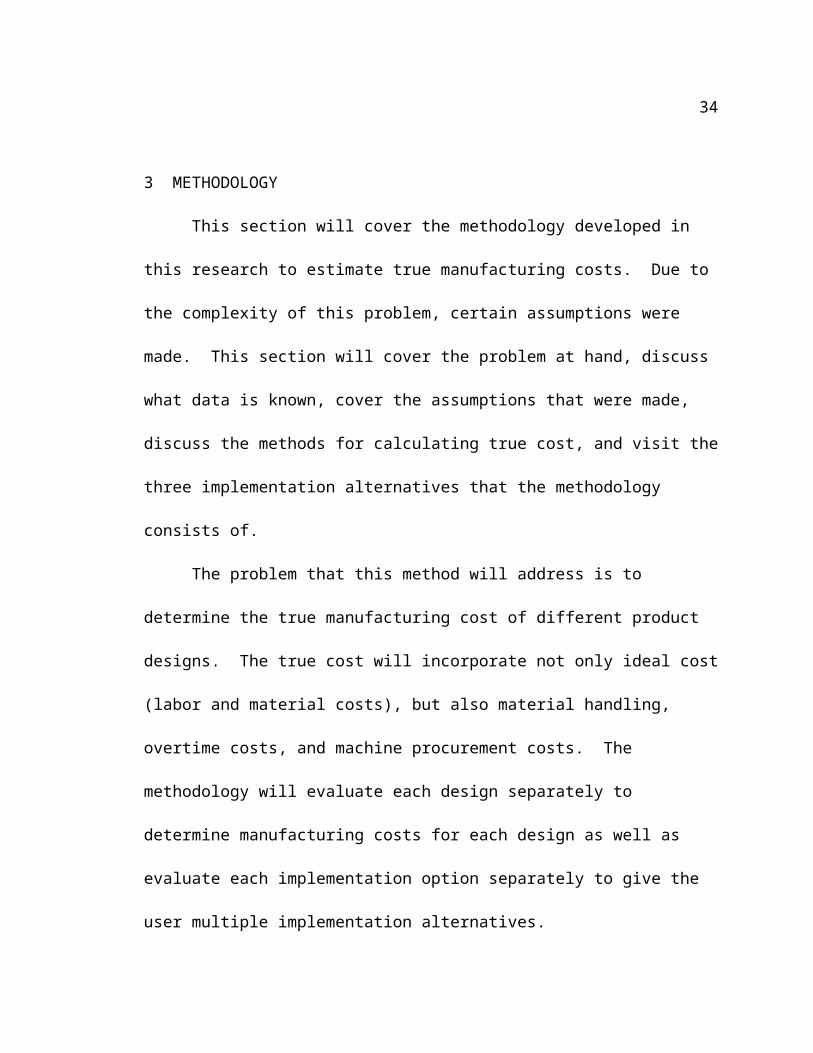
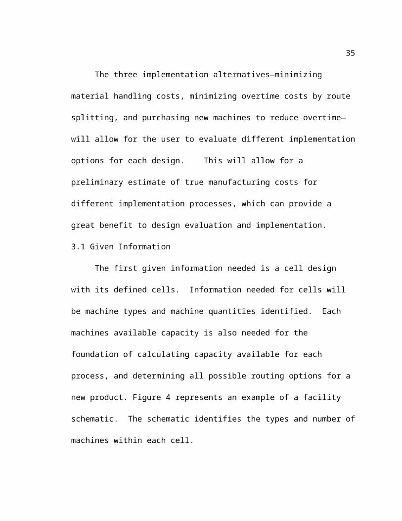
new product. Figure 4 represents an example of a facility schematic. The schematic

identifies the types and number of machines within each cell.

Cell 1 Cell 2

Cell 3 Cell 4

Cell 5

Machine E

Machine B

Machine E

Machine A

Machine E

Machine F

Machine A Machine C

Machine D Machine E

Machine C

Machine B

Machine B

Machine D

Machine F

Machine D

Machine C

Machine A

Machine A

Machine D

Figure 4: Example of Facility Schematic

25

The figure above identifies five cells, each with four machines. Cell 1 has

machines D, E, F, and A; cell 2 has machines C, E, B, and F; cell 3 has machines A, B, C,

and D; cell 4 has machines D, E, A, and B; cell 5 has A, C, D, and E. All cells in this

example have 4 machines, but this is not required.

The next pieces of information needed are the distances between those cells, to

determine material handling costs. The distance between cells is directly related to

material handling costs, meaning the longer the distance, the higher the cost.

Next, the processing time of each existing product is needed for each machine the

product is assigned to. The weekly demand for each product is also needed to calculate

remaining available capacity on each machine. It is important to know the current

production levels in the facility to accurately determine the time available for each

machine to process new parts.

Note, the same type of machines within a facility can vary in capacity available

depending on each individual machine’s load. Table 1 shows an example set of

processing times for the manufacturing system shown in Figure 4.

Cell

Part

Process 1 (hr/part)

Process 2 (hr/part)

Process 3 (hr/part)

Process 4

Total Processing Demand

26

(hr/part)

Time (hr/part)

(pts/wk)

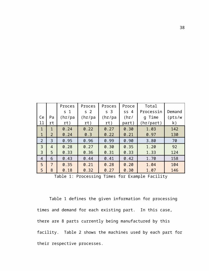
1 1 0.24 0.22 0.27 0.30 1.03 1421 2 0.24 0.3 0.22 0.21 0.97 1302 3 0.95 0.96 0.99 0.90 3.80 703 4 0.28 0.27 0.30 0.35 1.20 923 5 0.33 0.36 0.31 0.33 1.33 1244 6 0.43 0.44 0.41 0.42 1.70 1585 7 0.35 0.21 0.28 0.20 1.04 1045 8 0.18 0.32 0.27 0.30 1.07 146

Table 1: Processing Times for Example Facility

Table 1 defines the given information for processing times and demand for each

existing part. In this case, there are 8 parts currently being manufactured by this facility.

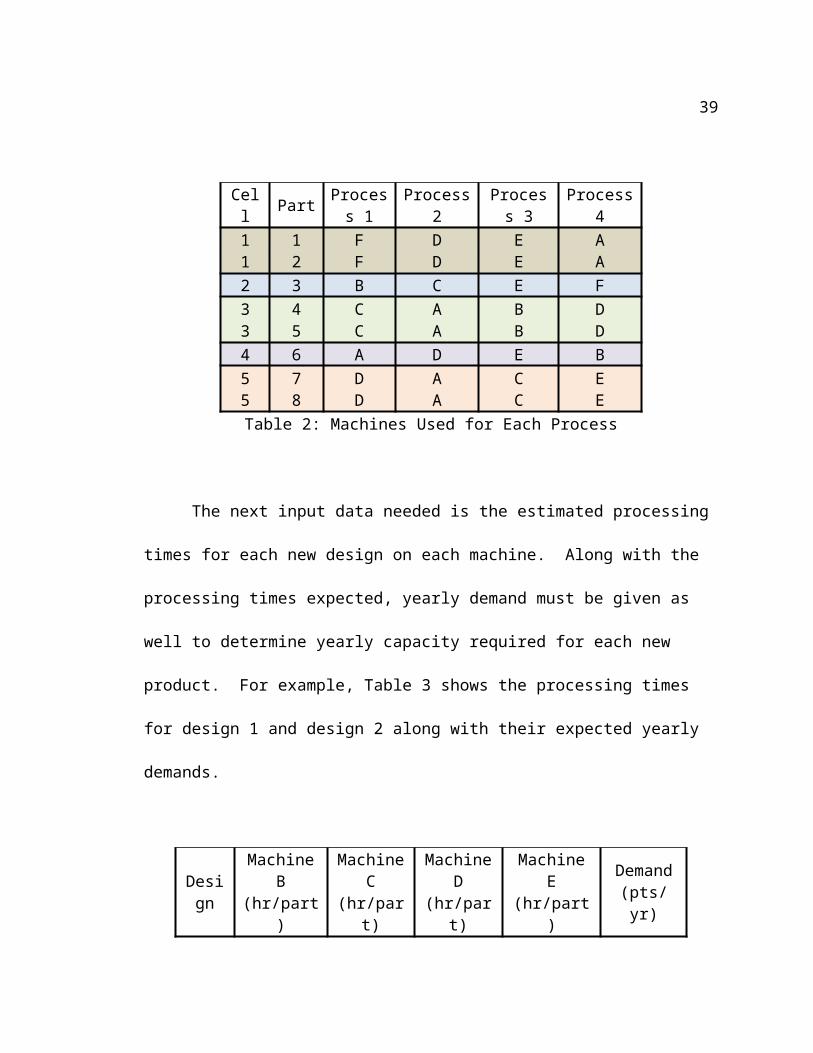
Table 2 shows the machines used by each part for their respective processes.

Cell Part Process 1 Process 2 Process 3 Process 4

1 1 F D E A1 2 F D E A2 3 B C E F3 4 C A B D3 5 C A B D4 6 A D E B5 7 D A C E5 8 D A C E

Table 2: Machines Used for Each Process

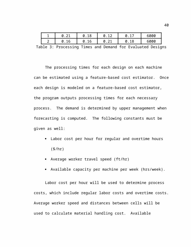
The next input data needed is the estimated processing times for each new design

on each machine. Along with the processing times expected, yearly demand must be

given as well to determine yearly capacity required for each new product. For example,

27

Table 3 shows the processing times for design 1 and design 2 along with their expected

yearly demands.

Design Machine B (hr/part)

Machine C (hr/part)

Machine D (hr/part)

Machine E (hr/part)

Demand(pts/yr)

1 0.21 0.18 0.12 0.17 60002 0.16 0.16 0.21 0.18 6000

Table 3: Processing Times and Demand for Evaluated Designs

The processing times for each design on each machine can be estimated using a

feature-based cost estimator. Once each design is modeled on a feature-based cost

estimator, the program outputs processing times for each necessary process. The demand

is determined by upper management when forecasting is computed. The following

constants must be given as well:

Labor cost per hour for regular and overtime hours ($/hr)

Average worker travel speed (ft/hr)

Available capacity per machine per week (hrs/week).

Labor cost per hour will be used to determine process costs, which include regular

labor costs and overtime costs. Average worker speed and distances between cells will

be used to calculate material handling cost. Available capacity per machine per week is

determined by the expected number of hours a machine is available during the week for

all shifts.

28

3.2 Assumptions

Due to the complexity of this problem, several assumptions were made to

simplify the problem. The first assumption applies to the layout of facilities. It will be

assumed that the facility in evaluation has a cellular layout. Cellular manufacturing is

when machines are grouped together according to part families into cells. Part families

are groups of parts that are similar in their required manufacturing processes. By

grouping these parts together, cells are formed and material flow, as well as lead time,

can be improved.

This methodology can be adapted to work with a job shop layout. Rather than

cells, the facility will be analyzed as a whole and the option with minimum overtime and

material handling will be the optimal solution. The methodology is not suggested for use

with a production line layout. When having cells and machines in different locations

around the facility, material handling will be present, moving from one cell to another.

Production lines lack the material movement, and therefore, would be unnecessary to try

and minimize material handling costs.

The next assumption that was made was that the demand for each existing and

proposed product is constant. The importance of this is to evaluate the product using the

best information available about demand.

The final assumption is a batch size of one for material handling. Assuming a

batch size of one denotes material handling will apply to each and every part that moves

from one cell to another. If batch size is greater than one, the number of material

handling trips would be divided by the batch size.

29

4 MODEL FOR TRUE COST

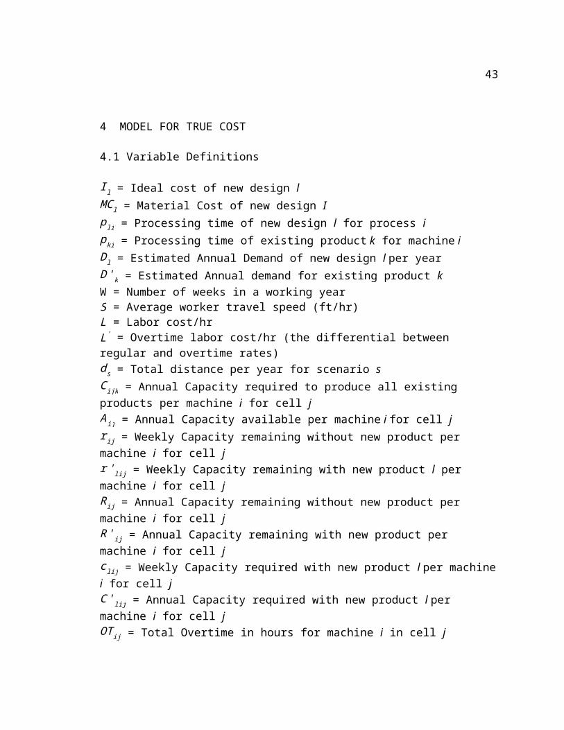
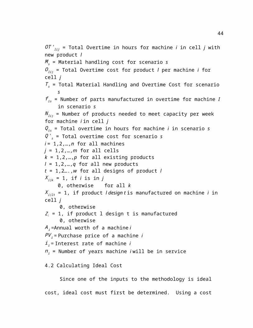
4.1 Variable Definitions

I l = Ideal cost of new design lMC l = Material Cost of new design Ipli = Processing time of new design l for process ipki = Processing time of existing product k for machine iDl = Estimated Annual Demand of new design l per yearD 'k = Estimated Annual demand for existing product kW = Number of weeks in a working yearS = Average worker travel speed (ft/hr)L = Labor cost/hrL' = Overtime labor cost/hr (the differential between regular and overtime rates)ds = Total distance per year for scenario sC ijk = Annual Capacity required to produce all existing products per machine i for cell jAij = Annual Capacity available per machine i for cell jrij = Weekly Capacity remaining without new product per machine i for cell jr 'lij = Weekly Capacity remaining with new product l per machine i for cell jRij = Annual Capacity remaining without new product per machine i for cell jR 'ij = Annual Capacity remaining with new product per machine i for cell jc lij = Weekly Capacity required with new product l per machine i for cell jC ' lij = Annual Capacity required with new product l per machine i for cell jOT ij = Total Overtime in hours for machine i in cell jOT 'lij = Total Overtime in hours for machine i in cell j with new product lM s = Material handling cost for scenario sOlij = Total Overtime cost for product l per machine i for cell jT s = Total Material Handling and Overtime Cost for scenario sf is = Number of parts manufactured in overtime for machine I in scenario sN lij = Number of products needed to meet capacity per week for machine i in cell j Qis = Total overtime in hours for machine i in scenario sQ 's = Total overtime cost for scenario si = 1,2,…,n for all machinesj = 1,2,…,m for all cellsk = 1,2,…,p for all existing productsl = 1,2,…,q for all new productst = 1,2….,w for all designs of product lX ijk = 1, if i is in j

0, otherwise for all kX ijlt = 1, if product l design t is manufactured on machine i in cell j

30

0, otherwiseZ¿ = 1, if product l design t is manufactured

0, otherwiseAi =Annual worth of a machine iPV i = Purchase price of a machine iii = Interest rate of machine ini = Number of years machine i will be in service

4.2 Calculating Ideal Cost

Since one of the inputs to the methodology is ideal cost, ideal cost must first be

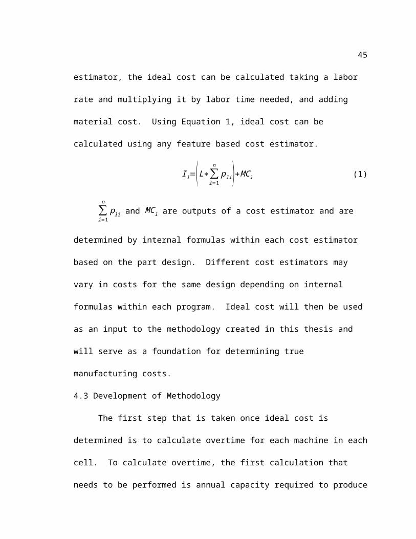
determined. Using a cost estimator, the ideal cost can be calculated taking a labor rate

and multiplying it by labor time needed, and adding material cost. Using Equation 1,

ideal cost can be calculated using any feature based cost estimator.

I l=(L∗∑i=1

n

pli)+MC l (1)

∑i=1

n

pli and MC l are outputs of a cost estimator and are determined by internal

formulas within each cost estimator based on the part design. Different cost estimators

may vary in costs for the same design depending on internal formulas within each

program. Ideal cost will then be used as an input to the methodology created in this

thesis and will serve as a foundation for determining true manufacturing costs.

4.3 Development of Methodology

The first step that is taken once ideal cost is determined is to calculate overtime

for each machine in each cell. To calculate overtime, the first calculation that needs to be

performed is annual capacity required to produce all existing products per machine per

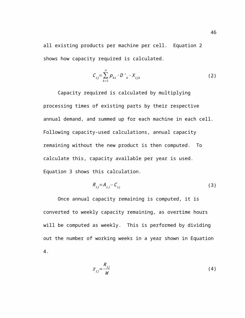
cell. Equation 2 shows how capacity required is calculated.

31

C ij=∑k=1

n

pki ∙ D ' k ∙ X ijk (2)

Capacity required is calculated by multiplying processing times of existing parts

by their respective annual demand, and summed up for each machine in each cell.

Following capacity-used calculations, annual capacity remaining without the new product

is then computed. To calculate this, capacity available per year is used. Equation 3

shows this calculation.

Rij=Ai j−C ij (3)

Once annual capacity remaining is computed, it is converted to weekly capacity

remaining, as overtime hours will be computed as weekly. This is performed by dividing

out the number of working weeks in a year shown in Equation 4.

r ij=Rij

W (4)

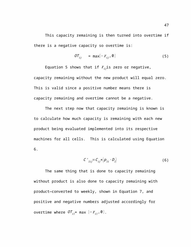
This capacity remaining is then turned into overtime if there is a negative capacity

so overtime is:

OT ij = max{−r ij ,0} (5)

Equation 5 shows that if r ijis zero or negative, capacity remaining without the new

product will equal zero. This is valid since a positive number means there is capacity

remaining and overtime cannot be a negative.

The next step now that capacity remaining is known is to calculate how much

capacity is remaining with each new product being evaluated implemented into its

respective machines for all cells. This is calculated using Equation 6.

C ' lij=C ij+( p li ∙ Dl ) (6)

32

The same thing that is done to capacity remaining without product is also done to

capacity remaining with product—converted to weekly, shown in Equation 7, and

positive and negative numbers adjusted accordingly for overtime where OT ij= max

{−r ij , 0}.

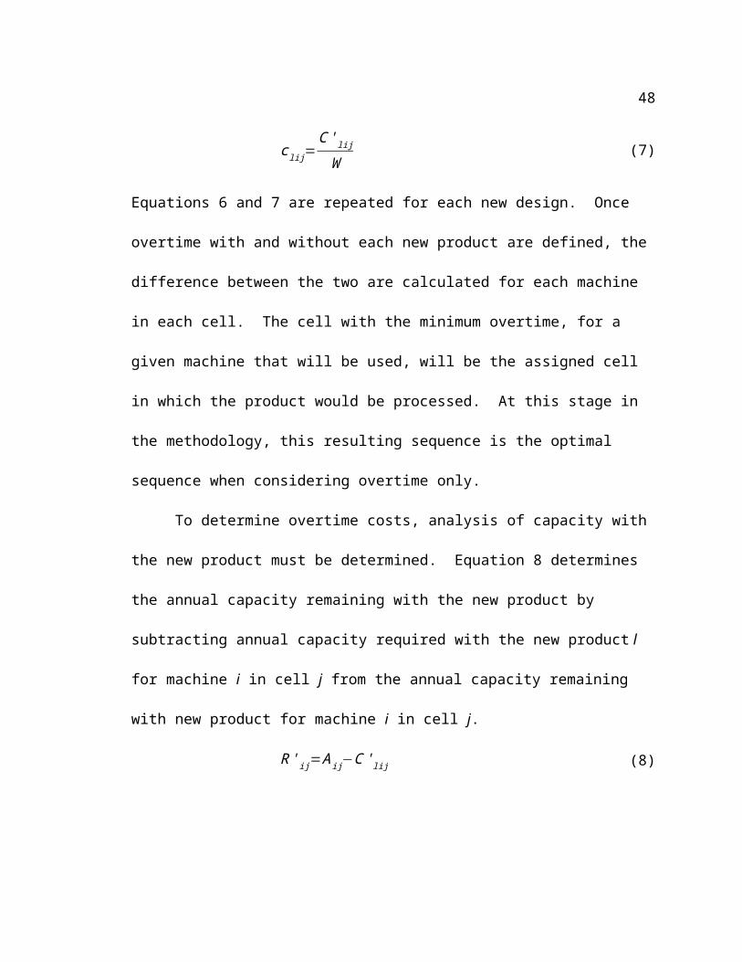
c lij=C ' lij

W (7)

Equations 6 and 7 are repeated for each new design. Once overtime with and without

each new product are defined, the difference between the two are calculated for each

machine in each cell. The cell with the minimum overtime, for a given machine that will

be used, will be the assigned cell in which the product would be processed. At this stage

in the methodology, this resulting sequence is the optimal sequence when considering

overtime only.

To determine overtime costs, analysis of capacity with the new product must be

determined. Equation 8 determines the annual capacity remaining with the new product

by subtracting annual capacity required with the new product l for machine i in cell j

from the annual capacity remaining with new product for machine i in cell j.

R 'ij=Aij−C 'lij (8)

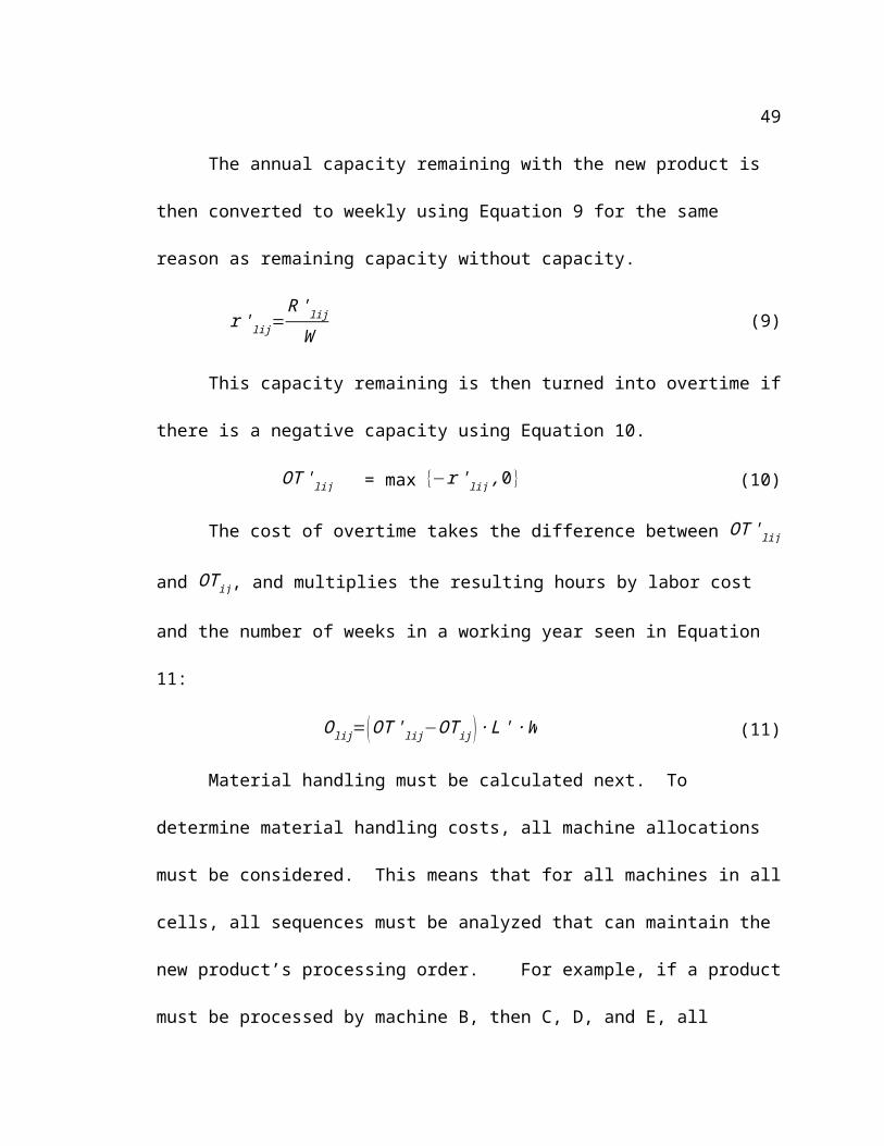
The annual capacity remaining with the new product is then converted to weekly

using Equation 9 for the same reason as remaining capacity without capacity.

r 'lij=R ' lij

W (9)

This capacity remaining is then turned into overtime if there is a negative capacity

using Equation 10.

33

OT 'lij = max {−r 'lij ,0 } (10)

The cost of overtime takes the difference between OT 'lij and OT ij, and multiplies

the resulting hours by labor cost and the number of weeks in a working year seen in

Equation 11:

Olij=(OT ' lij−OT ij) ∙ L' ∙ W (11)

Material handling must be calculated next. To determine material handling costs,

all machine allocations must be considered. This means that for all machines in all cells,

all sequences must be analyzed that can maintain the new product’s processing order.

For example, if a product must be processed by machine B, then C, D, and E, all

scenarios that can fulfill that order regardless of the cell will be analyzed for material

handling costs.

Once all scenarios are determined, material handling costs are calculated based on

number of cell-to-cell movements and distances between those cells for each scenario.

Total distances are calculated for each scenario, which will be used to directly compute

material handling costs for each scenario. Total distances per scenario will then be

multiplied by the product demand to convert to distance per year. Then material handling

cost calculations are computed using Equation 12.

M s=d s

S∙ L (12)

This material handling cost is then added to overtime cost for each scenario to get

T s, which allows the user to determine the best scenario to minimize manufacturability

costs. Once the scenario is identified and determined, the next step is to split the product

into multiple routes, creating less overtime, and increasing material handling.

34

4.4 Splitting Into Multiple Routes

A route in manufacturing can be defined as the path in which a product travels

through a facility in order to be manufactured. The route consists of all the machines

needed for the part to be manufactured. Splitting the product into multiple routes means

that some of the product will travel one route through the facility, some will travel

another route, and so on until there are enough routes to either eliminate overtime, or

minimize overtime. This in turn creates more intercellular movement increasing material

handling costs.

Using the scenarios from section 4.2 to calculate material handling, the scenarios

will be ordered from minimum M s to maximum M s to analyze the scenarios with

minimum material handling costs first. Once all scenarios have been ordered, the number

of products that can be produced without exceeding capacity for each machine per week

is then calculated. Calculations are done for each machine of each cell. This identifies

the maximum number of products that can be manufactured on the given machine before

overtime is needed. Using Equation 13, the number of products needed to meet capacity

can be determined.

N lij=r ' lij

pki (13)

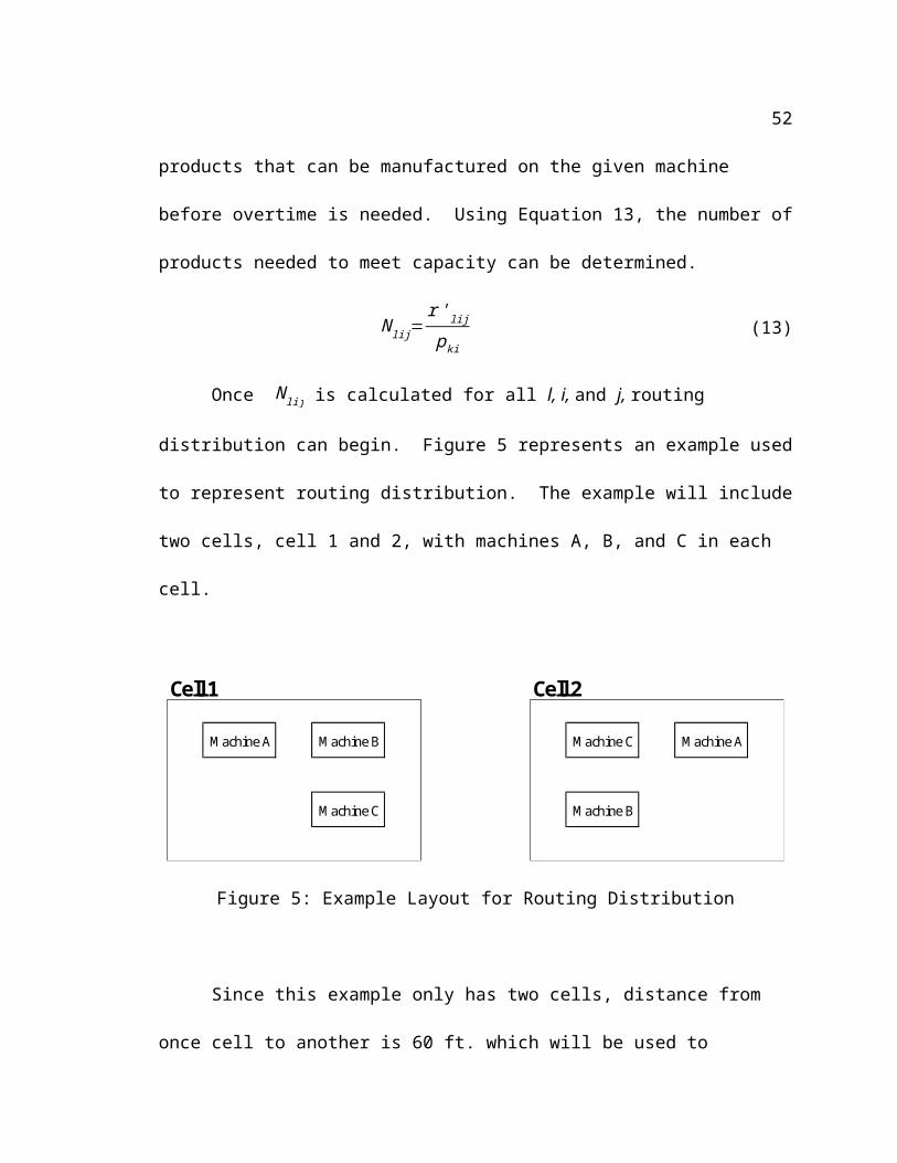
Once N lij is calculated for all l, i, and j, routing distribution can begin. Figure 5

represents an example used to represent routing distribution. The example will include

two cells, cell 1 and 2, with machines A, B, and C in each cell.

35

Cell 1 Cell 2

Machine AMachine A Machine B Machine C

Machine C Machine B

Figure 5: Example Layout for Routing Distribution

Since this example only has two cells, distance from once cell to another is 60 ft.

which will be used to calculate material handling costs for each scenario. The new

product will need Machine A, B, and C, with processing times and demand given as well,

to determine capacity remaining for each machine. Each possible scenario for production

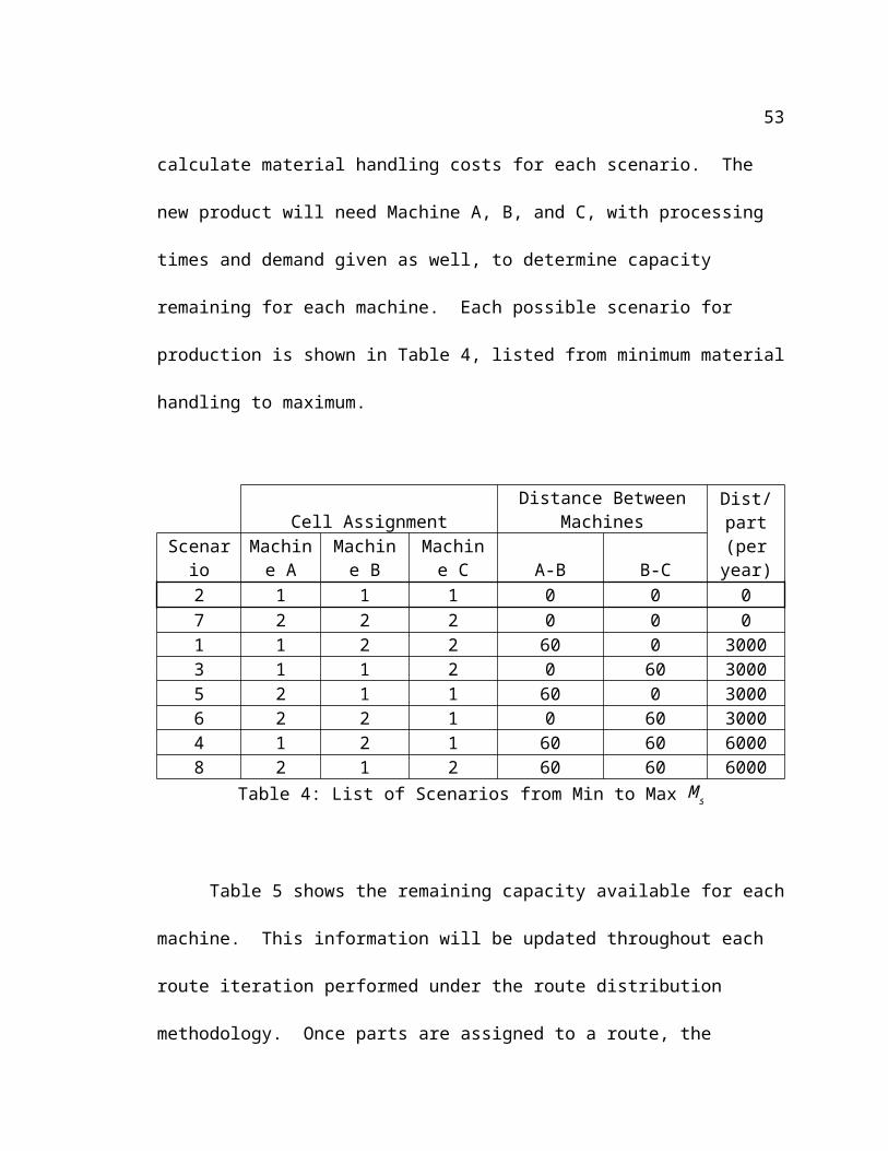
is shown in Table 4, listed from minimum material handling to maximum.

Cell AssignmentDistance Between

MachinesDist/part (per year)Scenario

Machine A

Machine B

Machine C A-B B-C

2 1 1 1 0 0 07 2 2 2 0 0 01 1 2 2 60 0 30003 1 1 2 0 60 30005 2 1 1 60 0 30006 2 2 1 0 60 30004 1 2 1 60 60 60008 2 1 2 60 60 6000

Table 4: List of Scenarios from Min to Max M s

36

Table 5 shows the remaining capacity available for each machine. This

information will be updated throughout each route iteration performed under the route

distribution methodology. Once parts are assigned to a route, the remaining capacity

available for each machine must be recalculated.

Machine (pts/wk)A B C

Cell 1 12 11 142 16 15 9

Table 5: Starting Capacity Available for Machines

Routing distribution will go as follows:

1. Choose the first route (with minimum M s)

Since the first route is chosen, Scenario 2 in the example will be chosen as shown

in Table 6. Machines A, B, and C in cell 1 will all be utilized for this iteration.


Machines Dist/part (per

year)Scenario

Machine A

Machine B

Machine C A-B B-C

2 1 1 1 0 0 07 2 2 2 0 0 01 1 2 2 60 0 30003 1 1 2 0 60 30005 2 1 1 60 0 30006 2 2 1 0 60 30004 1 2 1 60 60 60008 2 1 2 60 60 6000

37

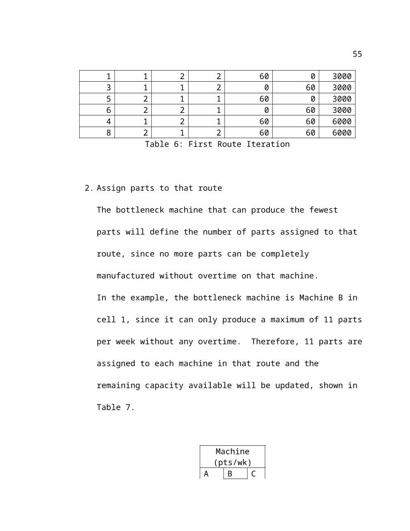
Table 6: First Route Iteration

2. Assign parts to that route

The bottleneck machine that can produce the fewest parts will define the number

of parts assigned to that route, since no more parts can be completely

manufactured without overtime on that machine.

In the example, the bottleneck machine is Machine B in cell 1, since it can only

produce a maximum of 11 parts per week without any overtime. Therefore, 11

parts are assigned to each machine in that route and the remaining capacity

available will be updated, shown in Table 7.


Cell1 1 0 32 16 15 9

Table 7: Remaining Capacity after First Iteration

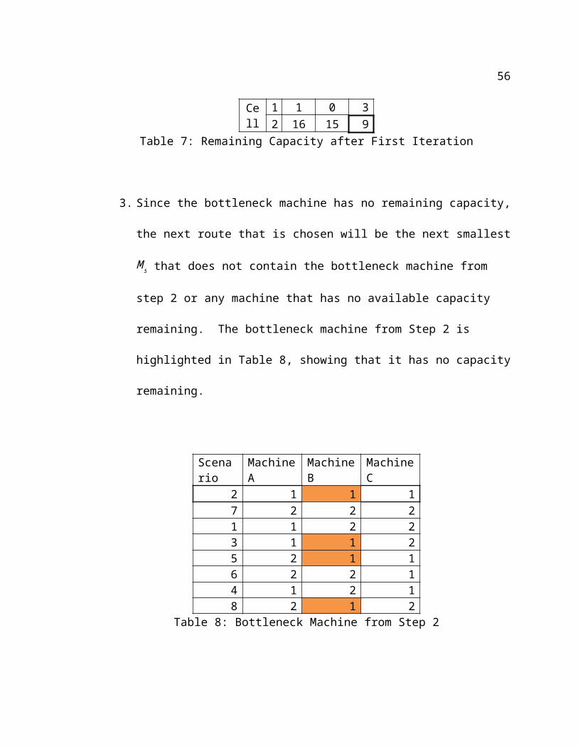
3. Since the bottleneck machine has no remaining capacity, the next route that is

chosen will be the next smallest M s that does not contain the bottleneck machine

from step 2 or any machine that has no available capacity remaining. The

bottleneck machine from Step 2 is highlighted in Table 8, showing that it has no

capacity remaining.

Scenario Machine A Machine B Machine C

38

2 1 1 17 2 2 21 1 2 23 1 1 25 2 1 16 2 2 14 1 2 18 2 1 2

Table 8: Bottleneck Machine from Step 2

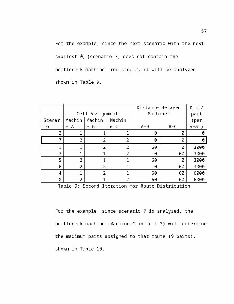
For the example, since the next scenario with the next smallest M s (scenario 7)

does not contain the bottleneck machine from step 2, it will be analyzed shown in

Table 9.


MachinesDist/part (per year)Scenario

Machine A

Machine B

Machine C A-B B-C

2 1 1 1 0 0 07 2 2 2 0 0 01 1 2 2 60 0 30003 1 1 2 0 60 30005 2 1 1 60 0 30006 2 2 1 0 60 30004 1 2 1 60 60 60008 2 1 2 60 60 6000

Table 9: Second Iteration for Route Distribution

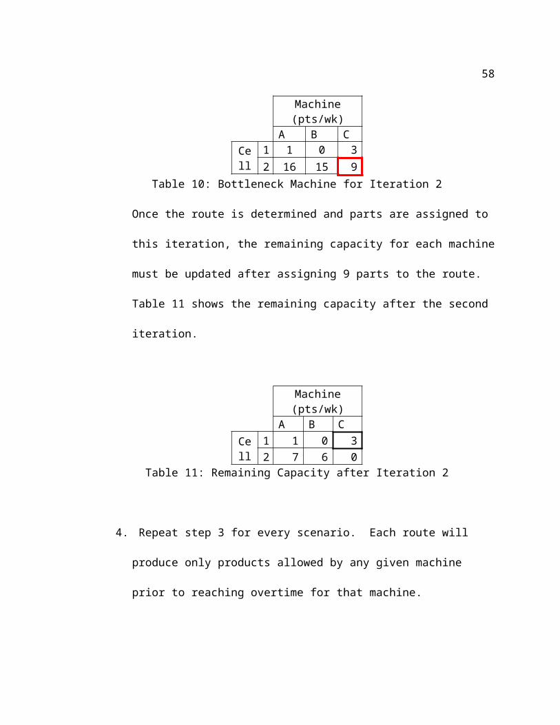
For the example, since scenario 7 is analyzed, the bottleneck machine (Machine C

in cell 2) will determine the maximum parts assigned to that route (9 parts),

shown in Table 10.

39


Cell1 1 0 32 16 15 9

Table 10: Bottleneck Machine for Iteration 2

Once the route is determined and parts are assigned to this iteration, the remaining

capacity for each machine must be updated after assigning 9 parts to the route.

Table 11 shows the remaining capacity after the second iteration.


Cell1 1 0 32 7 6 0

Table 11: Remaining Capacity after Iteration 2

4. Repeat step 3 for every scenario. Each route will produce only products allowed

by any given machine prior to reaching overtime for that machine.

If demand has been met, then the multiple scenario analysis is complete. If

demand is not met, proceed to step 5.

(Since capacity has not been met on all machines and overtime must be used, the

goal is to then minimize material handling since overtime will remain constant

regardless of what route will be chosen.)

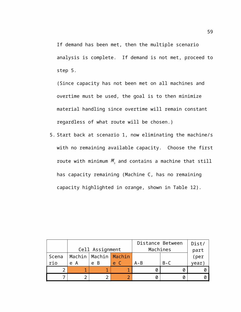
5. Start back at scenario 1, now eliminating the machine/s with no remaining

available capacity. Choose the first route with minimum M s and contains a

machine that still has capacity remaining (Machine C, has no remaining capacity

highlighted in orange, shown in Table 12).

40


Machines Dist/part (per

year)Scenario

Machine A

Machine B

Machine C A-B B-C

2 1 1 1 0 0 07 2 2 2 0 0 01 1 2 2 60 0 30003 1 1 2 0 60 30005 2 1 1 60 0 30006 2 2 1 0 60 30004 1 2 1 60 60 60008 2 1 2 60 60 6000

Table 12: Eliminate Machine from Analysis

Note: Scenario 7 was chosen due to the unavailability of Machines A and B in

Cell 1. Although scenario 2 would have been the first choice, we must analyze a

scenario will capacity remaining for both machines A and B, ignoring machine C.

6. Assign parts to that route

After step 4, the remaining capacity is shown in Table 13.


Cell1 0 0 02 4 3 0

Table 13: Remaining Capacity for Step 6

41

Using Table 13, the bottleneck machine for scenario 7 is Machine B in cell 2.

Therefore, 3 parts will be assigned to this iteration.

7. Choose the next route in succession with minimum M s and contains machines

that still have capacity remaining and assign parts to that route. Repeat this step

until all demand has been met or all possible scenarios have been analyzed. If

demand has not been met, proceed to step 8.

8. Once capacity has been met, manufacture the remaining parts on the scenario with

minimum M s since no option is left but overtime on all machines, shown in Table

14.


Machines Dist/part (per year)Scenario

Machine A

Machine B

Machine C A-B B-C

2 1 1 1 0 0 07 2 2 2 0 0 01 1 2 2 60 0 30003 1 1 2 0 60 30005 2 1 1 60 0 30006 2 2 1 0 60 30004 1 2 1 60 60 60008 2 1 2 60 60 6000Table 14: Assign remaining demand to Scenario with minimum M s

Since all machines have been fully utilized up to capacity, manufacturing the

remaining parts will require overtime anyways, so the key is to then reduce material

42

handling by choosing the scenario with minimum M s. The final result of the route

distribution for the example above is shown in Table 15.

Iteration ScenarioParts

Assigned Distance/yr Overtime Costs1 2 11 0 02 7 9 0 03 6 3 3000 3 parts4 7 3 6000 3 parts5 7 1 3000 2 parts6 2 31 0 31 parts

Table 15: Results from Routing Example

Once the steps have been performed, a total cost analysis will be performed for

the route splitting analysis. Table 16 shows the final cost analysis results for material

handling and overtime costs.

Overtime (parts) Overtime (hours)

Itera

tion

Scen

ario

Part

s Ass

igne

d

Dist

ance

/yr

Mac

hine

A

Mac

hine

B

Mac

hine

C

Mac

hine

A

Mac

hine

B

Mac

hine

C

Total Overtime Cost/yr

Total Matl. Hand

Cost/yr

1 2 11 0 0 0 0 $0 $02 7 9 0 0 0 0 $0 $0

3 6 3900

0 0 0 0 $0 $1534 7 3 0 3 0 0 171 $5,130 $05 7 1 0 1 1 0 51 57 $3,240 $0

6 2 31 0 31 31 311317.

5158

1176

7 $139,965 $0total $148,335 $153total $148,488

43

Table 16: Total Cost Results for Route Splitting

Table 16 is created by analyzing each iteration performed. Distance per year is

calculated the same way as Table 4 for each scenario and converted into cost by

multiplying distance per year by the number of parts assigned for each scenario. The

number of parts manufactured in overtime for each machine equals the number of parts

assigned to that iteration if Rij= 0 for each machine. Once the number of parts

manufactured in overtime for each machine is determined, the parts are then converted to

time in hours using Equation 14.

Qis=f is∗pli∗W (14)

Total overtime cost for each scenario is then calculated using Equation 15.

Q 's=(∑i=1

n

Ois)∗L ' (15)

Material handling costs and overtime costs for each iteration is then added up and

totaled at the lower right hand of Table 16. The total cost for route splitting is $148,488.

4.5 Purchasing Machines

The next part of the methodology will evaluate purchasing additional machines

and its effect on manufacturing costs. Purchasing new machines will allow more

available capacity in the facility, reducing total overtime costs. Although the addition of

more machines will reduce overtime costs, new machines will also require more upfront

purchasing costs that will need to be accounted for. This methodology will test whether

adding a machine will reduce operating costs—including overtime and material handling

—in order to offset the purchasing costs.

44

To demonstrate this step of the methodology, the example from Section 4.4 will

be used. The same layout will be used from Figure 5 in Section 4.4, using 2 cells, each

cell containing a Machine A, B, and C. Table 5 shows the remaining capacity available

for each machine in each cell.

Like Table 3 in Section 3.1, the input data needed is the estimated processing

times on each machine for the new part designs being evaluated. Yearly demand must be

given as well and this data will be used to determine weekly capacity required for the

new product. For this example, the new product will have the following given

information in Table 17.

A B C Demand (yr)

Processing time 0.85 hr 1.02 hr 1.14 hr 2900

Table 17: Processing Times and Demand of New Product

This example will be used to test three separate options: adding a Machine A,

adding a Machine B, and adding a Machine C. First, purchasing cost must be identified.

In order to analyze the purchasing cost of a machine, several factors need to be addressed

to convert a machine’s present value worth into an annual cost per year. This is needed

because manufacturing costs are calculated on an annual basis. To convert the present

value, the purchase cost (present value worth), life span (number of years), and interest

rate of the machine will be needed. Once the information is known, annual cost can be

calculated using Equation 16.

45

A=PV i (1+i )n

(1+i )n−1 (16)

When adding a machine to a facility, it will increase the amount of remaining

capacity available for that specific process the machine will provide. This will allow for

more resource availability allowing more parts to be manufactured in a given week.

Table 5 shows the initial remaining capacity for Machine A, B, and C, in both cells 1 and

2. If another unit of Machine A is purchased and can run for 40 hours a week, at 0.85

hours processing time per part from Table 17, the machine has enough capacity to

produce 47 additional parts per week.

The 47 additional parts a week will then be added to the existing capacity of

Machine A shown in Table 5 in the cell that is least utilized. This will allow for optimal

utilization of capacity, reducing overtime costs. The results can be seen in Table 18 ,

where the 47 additional parts have been added to Cell 1, highlighted.


Cell 1 59 11 142 16 15 9

Table 18: Starting Capacity Available with Additional Machine A

With this updated starting capacity, routing distribution from Section 4.3 will be

performed. Once steps 1 through 9 have been completed, a total cost analysis will be

performed. For each iteration of steps 1 through 9, an overtime cost and material

handling cost is calculated shown in Table 19.

46

Overtime (parts) Overtime (hours)

Itera

tion

Scen

ario

Part

s Ass

igne

d

Dist

ance

/yr

Mac

hine

A

Mac

hine

B

Mac

hine

C

Mac

hine

A

Mac

hine

B

Mac

hine

C

Total Overtime Cost/yr

Total Matl. Hand

Cost/yr

1 2 11 0 0 0 0 $0 $02 7 9 0 0 0 0 $0 $0

3 6 3900

0 0 0 0 $0 $1534 7 3 0 3 0 0 171 $5,130 $0

5 2 32 0 32 32 0163

2182

4 $103,680 $0total $108,810 $153total $108,963

Table 19: Total Overtime and Material Handling cost with Additional Machine A

Table 19 provides the same analysis for routing splitting with additional machines

as Table 16 does for route splitting in Section 4.4. Material handling costs and overtime

costs for each iteration is are added up and totaled. The total cost of $108,963 is then

added to the procurement cost of Machine A calculated using Equation 10. For equation

10, Machine A will have a purchasing cost of $150,000, a life span of 10 years, and an

47

interest rate of 20%. This will provide an annual cost of $35,779. Therefore, the total

cost with an additional Machine A will be $144,742.

This process is done for Machines B and C as well. Their total costs will be

calculated and compared with each other as well as the total cost without adding an

additional machine.

4.6 Product Selection Optimization

The methodology proposed can provide benefit to multiple design analysis. To

even further the extent to which the methodology can be used, a math model has been

created to optimize product selection. The methodology allows the user to evaluate

multiple different designs of a given product, while the math model will allow the user to

determine product selection if there is more than one product to manufacture.

In real world scenarios, it is likely a company may have multiple products to

manufacture and must determine which, if any, would provide the most profit to the

company. It can be difficult to understand profit without knowing the cost to

manufacture the product, especially needing true cost of the product. By optimizing

product selection, the model can determine which product or combination of products to

manufacture to optimize profits.

The math model uses the cost output of the methodology from alternative 1 as an

input to the model. This will allow the model to analyze true manufacturing costs for

each product, for optimal selection. By evaluating true cost in product selection, users

can more accurately determine profit values than by using ideal cost. This provides

48

benefit to not only design analysis, but product selection as well, making the

methodology even more versatile.

4.6.1 Math Model

The objective function of the math model maximizes profit by subtracting the cost

of products from the revenue of the products, shown in (17).

P=∑l∑

t(S¿−I ¿ )∗1.15 Z¿

(17.1)

−∑i∑

jOij∗1.15 (17.2)

−∑l∑

tM ¿∗1.15 (17.3)

The objective function consists of three components: the selling price minus the

ideal manufacturing cost (17.1), overtime cost (17.2), and material handling cost (17.3).

The constraints for the formulation are as follows:

C 'ij=∑

l∑

t(C ijk+( Pil∗Dl ))∗X ijlt

(18)

R 'ij=Aij−C 'ij (19)

Oij=(max {−R 'ij , 0 }−max {−R ij , 0})∗L' (20)

d¿=∑i=2

n

∑j=1} to {m} {sum from {j=1} to {m} {{d} rsub {j {j} ^ {'}} {X} rsub {ijlt} {X} rsub {{i-1} rsub {j<¿

¿¿(21)

M ¿=d¿

S∙ L

(22)

∑i∑

jX ijlt=m¿∗Z¿

(23)

49

The objective function takes ideal cost, material cost, and overtime cost and subtracts

the cost from the selling price of a product, resulting in profit. The costs are multiplied

by 1.15 to account for amount of acceptable profit of at least 15% of the cost. The model

will assume any product that has a selling price higher than its cost will be chosen to

manufacture. By multiplying in a factor of 1.15, the model will not accept anything

lower than 15% gain, which would account for the practicality of earning enough profit

to make the product worth manufacturing.

Constraint (18) calculates annual capacity required with the new product l for

machine i in cell j. This is needed to calculate constraint (19), which calculates annual

capacity remaining for machine i in cell j if design t product l is manufactured. Once

annual capacity remaining is determined, annual cost of overtime (20) is calculated for

machine i in cell j if design t product l is manufactured. Constraint (21) calculates total

distance required per year for design t product l, which is then used in constraint (22) to

determine material handling for design t product l.

An OPL model was created to test results. For simplicity purposes, the data used

represents a facility with only one cell, so material handling will be negligible. The data

includes the evaluation of implementing three different products, each with two designs.

There are a total of 6 machines in the facility. Processing times and processes needed for

each design are given and shown in the model attached in Appendix A.

50

The results indicate that the methodology demonstrated in this paper can be used in a

variety of applications, not only for its purpose to provide design selection and possible

implementation options, but also using true cost as inputs to other methodologies in

manufacturing. The methodology can be a great tool is using true manufacturing costs to

determine a variation of manufacturing cost problems, such as this model for product

selection to optimize profits. This model represents just one of many options how true

manufacturing cost estimation can add value to cost calculations.

5 EVALUATION OF MULTIPLE DESIGNS

To better demonstrate the proper use of this methodology, different designs for

the same part will be analyzed. By analyzing two separate designs for the same part, the

methodology can be used to not only determine the cheapest design, but also to determine

the cheapest way to implement the design by analyzing the three alternative

implementations. Determining costs for manufacturing new product designs can provide

valuable manufacturing information to designers.

Using this example, by analyzing multiple designs, will show how this valuable

information can provide an easy guideline to determine which design will be cheaper to

manufacture and implement given the current system capacity and providing three

implementation alternatives to minimize costs.

5.1 Ideal Cost Derivation

This example is modeled after a real-life example used with Ohio University’s

cost estimation research with jet engine components. The two designs that will be used

51

are examples of jet engine components. To evaluate the two designs, the ideal cost must

first be calculated using a feature-based cost estimator.

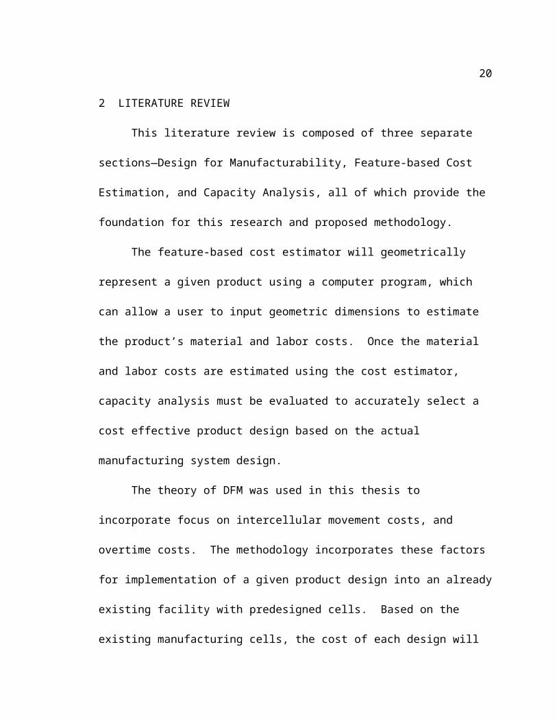
Ohio University’s cost estimator is a feature-based cost estimator, which analyzes

part designs by evaluating each individual feature. The cost estimator provides an

estimate of process time per feature, and breaks down the manufacturing cost for each

feature. Figure 6 shows the breakdown of a part and its features using the cost estimator.

Figure 6: Cost Estimator Breakdown

52

In the breakdown in Figure 6, the features have been itemized, with the cost of

each feature being determined separately. For confidentiality reasons, the costs have

been erased from the figure. Once the cost of each feature has been estimated, the costs

are accumulated and totaled to provide the ideal manufacturing cost.

This cost estimator could be used to generate the ideal costs for each design used

in the example. Once the ideal cost is calculated, the methodology is used to calculate

true manufacturing costs for each alternative. Since there are three alternatives for each

design, there are a total of 6 possible options to minimize costs.

5.2 Problem Overview

The first aspect of the problem that needs to be addressed is given information.

The same information needed from Section 3.1 is required for this example—cell design;

system capacity, processes required and processing times for each; and demand for the

new product. Assumptions will remain the same from Section 3.2 as well.

The manufacturing system for this problem is shown in Figure 7. The system

consists of two cells with four machines in each cell. The shading represents the current

capacity used for each machine per day. The empty space in each machine is how much

capacity per day is still remaining until the machine reaches overtime. A completely

shaded machine has 0% capacity remaining, while a machine with no shade has 100%

capacity remaining.

53

Figure 7: Cell Design

The two designs that will be analyzed in this example are both similar in design

by looks and weight. It would be difficult to distinguish differences in manufacturing

costs from one another only from the drawings. In order to distinguish the cost

differences, the designs along with other given information need to be specified. Shown

in Figure 8, designs A and B can be seen as generated by feature based cost estimator.

54

Figure 8: Multiple Design Example

Design A will require Machines A, D, and F, with processing times of 2.1 hrs, 3.6

hrs, and 0.9 hrs respectively while Design B will require Machines B, C, and E with

processing times of 3.9 hrs, 2.4 hrs, and 1.5 hrs. The total processing time for Design A

is 6.6 hours while Design B is 7.8 hours, each having an expected yearly demand of 500.

The breakdown of these processes and their times are shown in Table 20.

Design A Design BMachine Processing Time

Machine Processing Time

Process 1 A 2.1 (hrs) B 3.9 (hrs)Process 2 D 3.6 (hrs) C 2.4 (hrs)Process 3 F 0.9 (hrs) E 1.5 (hrs)Total 6.6 (hrs) 7.8 (hrs)

Table 20: Processes and Processing Times for New Designs

55

The feature-based cost estimator would calculate these times and uses this

information to return an estimate for ideal cost for each design using Equation 1. The

total processing time is multiplied by a fixed labor cost per hour (in this case $75/hr), and

added to material cost. Material cost is based on the amount of material used for each

design. Design A is $760/unit, while material cost for Design B is $731/unit. Therefore,

by using the feature base cost estimator to calculate ideal cost for each design, Design A

has an ideal cost of $1225/unit and Design B has $1316/unit, making Design A the

cheaper option. These costs are shown in Table 21.

Design A Design BLabor Cost $495 $585 Material Cost $760 $731 Ideal Cost $1,255 $1,316 Ideal Cost / year $627,500 $658,000

Table 21: Breakdown of Ideal Cost for New Designs

Due to comparing these results to other alternatives in the methodology, costs will

be compared as annual costs. This thesis will use annual cost in order to adequately

evaluate route splitting costs. Route splitting can’t be evaluated on a weekly basis. To

determine the optimal routes, calculations to meet a yearly demand must be met. It is

also more feasible to compare yearly costs vs. weekly costs as weekly costs are much

smaller and will not vary greatly from one alternative to another. Comparing yearly costs

shows differences in costs significantly more than weekly analysis. Annual costs are also

more feasible to companies when looking at finances based on the fiscal year.

56

5.3 Calculations

The next step is to analyze the three implementation alternatives for each design

to evaluate the optimal design and implementation solution. The three implementation

options that will be evaluated for each design are: (1) assigning a design to only one cell,

minimizing complexity and intercellular movements; (2) route splitting to minimize

overtime; and (3) adding machines to increase capacity for a given process.

5.3.1 Alternative 1: Assigning Design to Minimal Number of Cells

The first alternative will be analyzed by calculating overtime hours for each

machine in each cell if the new product is assigned to that cell. Using the methodology

from Section 4.3, Design A gets assigned to Machine A and D in cell 1, and Machine F in

cell 2, while Design B is assigned to Machines B and C in cell 1, and Machine E in cell 2,

as shown in Figure 9. The designs aren’t assigned to a single cell because neither cell has

all necessary machines to manufacture a product. Therefore, multiple cells must be used

in the production of each part.

57

Figure 9: Alternative 1 implementation

Interpreting Figure 9, the grey shows the processing time of Design A on each

machine, and the light red shows the processing time of Design B for each machine per

day. This was determined using a yearly demand of 500 parts per year, with a 50

week/5 day working year, which averages out to needing to manufacture two products

each day to meet demand. If capacity is still remaining for a machine, white space can be

seen, as shown in Machine E—since it has not used up all capacity, overtime remains 0

for that machine. If capacity is completely used up, the colors will reach the top of each

machine box, and extend even further to show overtime. Overtime per day in hours will

be 3.9, 5.8, and 0.1 for Design A in Machines A, D, and F, respectively, while Design B

will have 3 hours each for both Machines B and C.

58

Once overtime is determined, material handling costs are evaluated. From Figure 9,

material handling can be seen where green arrows have been assigned. This shows when

a design has to move from one cell to another, to complete manufacturing. Cell to cell

material handling costs are calculated using Equation 9. Once material handling costs are

computed, they are added to overtime costs and ideal costs to return a cost value for

implementation alternative 1. Table 22 shows the results for each design.

Design A Design BIdeal Cost $1,255 $1,316

Overtime Cost $155 $85Material Handling Cost $30 $30

Total True cost $1,440 $1,431True cost/year $720,000 $715,500

Table 22: Implementation Alternative 1 Results

Note that originally, Design A provided the least expensive design based on ideal cost.

Now that overtime and material handling costs have been analyzed, the results indicate

Design B is the least expensive design at $715,500. Now that alternative 1 results have

been calculated, route splitting will be investigated for further cost optimization options.

5.3.2 Alternative 2: Route Splitting

The second alternative will analyze the implementation of multiple routes,

thereby increasing material handling costs, but reducing overtime costs by using all

resources available. Using the methodology from Section 4.3, route splitting is

performed and four possible routes are determined, shown in Figure 10.

59

Figure 10: Possible Routes for Example

The four routes are identified by the arrows; each color is a separate route. The dotted

lines indicate movement within a cell, and the solid lines indicate movement between

cells. There are two routes for design A—blue and green, while the red and black routes

are for design B. Continuing with the route splitting methodology for Section 4.3, the

iterations are performed and a total cost for route splitting is calculated for each design.

Tables 23 and 24 show the iterations performed for each design and their respective

overtime and material handling costs for each.

60

Iteration # PartsMaterial Handling Cost / year

Overtime Cost / Iteration

Total Cost/ Iteration

1 35 $1,050 $0 $1,0502 62 $3,720 $0 $3,7203 52 $1,560 $3,276 $4,8364 21 $1,260 $1,512 $2,7725 330 $9,900 $46,480 $56,380

Total $68,758Table 23: Route Splitting Iteration Summary for Design A

Iteration # PartsMaterial Handling Cost / year

Overtime Cost / Iteration

Total Cost/ Iteration

1 208 $6,240 $0 $6,2402 250 $7,500 $0 $7,5005 42 $1,260 $3,024 $4,284

Total $18,024Table 24: Route Splitting Iteration Summary for Design B

From Tables 23 and 24, total overtime and material handling costs for designs A

and B are $68,758 and $18,024 respectively. Using ideal cost from Table 21, a total

manufacturing cost for each design can be calculated. Adding these ideal costs to the

overtime and material handling costs calculated through route splitting generate a true

cost of $696,258 and $676,024 for design A and B. These costs are shown in Table 25.

Design A Design BOT and MH $68,758 $18,024Ideal Cost $627,500 $658,000True Cost $696,258 $676,024

Table 25: Total Route Splitting Costs

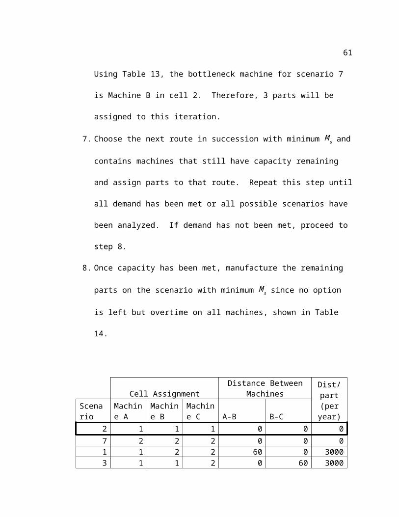
61

By using this implementation alternative, Design B is the optimal choice for route

splitting implementation with a cost of $676,024.

5.3.3 Alternative 3: Adding Machine/s Alternative

The third alternative will look at total costs when adding new machines to the

system, creating more available capacity. Using the methodology from Section 4.5,

alternative three will evaluate the costs of adding one of each of the machines being used

in the manufacturing processes for each design.

For simplicity purposes, this example will assume equal annual costs of each

machine. To determine the annual cost of each machine, Equation 16 will be used to

convert the machine procurement cost to an annual cost. With a procurement cost of

$200,000, an interest rate of 20% and a lifespan of 5 years, the annual cost of each

machine will be $66,876.

Once the annual cost of each machine is known, adding each machine will be

analyzed individually. Since three machines are used for each design A and B, a total of

six possible options will be looked at. With a total of 8 hours a day and 250 days a year,

each machine added will allow 2000 more available hours each year for that given

process. Table 26 through Table 31 shows the results calculated for each option.

Iteration AssignedMaterial Handling Overtime Total

1 97 $2,910 $0 $2,9102 403 $12,090 $43,524 $55,614

$58,524Table 26: Adding Machine A Results

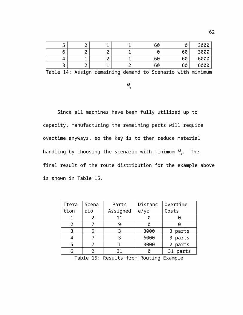
62


1 35 $1,050 $0 $1,0502 62 $1,860 $0 $1,8603 176 $5,280 $19,008 $24,2884 227 $6,810 $38,817 $45,627

$72,825Table 27: Adding Machine F Results


1 35 $1,050 $0 $1,0502 238 $7,140 $0 $7,1403 227 $6,810 $14,301 $21,111

$29,301Table 28: Adding Machine D Results


1 208 $6,240 $0 $6,2402 250 $7,500 $0 $7,5003 42 1,260 3,024 4,284

$18,024Table 29: Adding Machine B Results


1 500 $15,000 $0 $15,000 $15,000

Table 30: Adding Machine C Results


1 208 $6,240 $0 $6,240

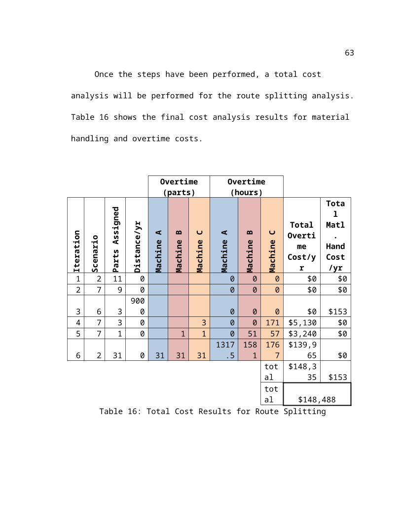
63

2 250 $7,500 $0 $7,5003 42 1,260 3,024 4,284

$18,024Table 31: Adding Machine E Results

Once results have been calculated for each option, ideal cost for each design along

with each machine’s annual worth will be added to compare total costs with other

alternatives. Table 32 shows the total cost results for each additional machine option.

Machine

M/C Cost

Ideal Cost

MH & OT Cost

Total Cost

Design A

A $66,876

$627,500 $58,524 $752,90

0

F $66,876

$627,500 $72,825 $767,20

1

D $66,876

$627,500 $29,301 $723,67

7

Design B

B $66,876

$658,000 $18,024 $742,90

0

C $66,876

$658,000 $15,000 $739,87

6

E $66,876

$658,000 $18,024 $742,90

0Table 32: Results of Additional Machines

Since all total costs are higher than alternative 2 results, there is no need for

further evaluation of additional machines. If any results indicated cheaper results than

the other two alternatives, multiple machine additions will need to be evaluated within

each design.

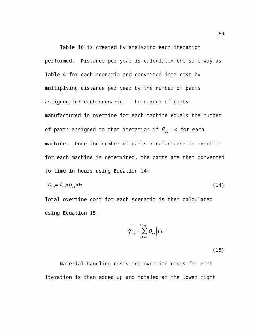
64

For instance, if both adding Machines A and D yielded cheaper costs than

alternative 1 or 2, another iteration for adding both machines will need to be evaluated.

This will verify if purchasing both machines will produce even less total costs.

In addition to evaluating multiple different machines, adding multiples of the

same machine must also be evaluated if an option yielded cheaper costs than alterative 1

or 2. Since all options yield higher costs than alternative 2, no further analysis is

required.

Evaluating the results from all options for alternative 3, the lowest cost option will

be chosen to compare with other alternative results. For this example, choosing Design A

and adding machine D is the cheapest at $723,677.

5.3.4 Evaluating Results

Now that all three alternatives have been looked at, the minimum total cost option

for each alternative will be compared to one another, and the overall cheapest option will

provide the optimal design and implementation. Gathering all the data from each

alternative, Table 33 shows the cheapest options for each alternative.

Alternative Design Ideal Cost Total Cost

1A $627,500 $720,000 B $658,000 $715,500

2A $627,500 $696,258 B $658,000 $676,024

3A $627,500 $723,677 B $658,000 $739,876

Table 33: Example Results

65

Implementing design B using alternative 2 route splitting is identified as the

optimal solution for this example. This indicates that route splitting Design B will have

the least amount of manufacturing costs at $676,024 a year.

This example shows how ideal costs can provide an underestimation of

manufacturing costs and how important it can be to consider true costs. Using Table 33,

ideal costs are shown with their respective design/alternative along with true costs

calculated using the methodology. Ideal cost is shown as constant regardless of the

implementation method. Using the methodology to estimate true cost provides more in

depth analysis to manufacturability. If ideal cost was used, Design A would be

considered to implement due to lowest cost. Looking further into true cost, one would

now consider Design B as the cheapest option when considering other manufacturability

factors such as overtime and material handling.

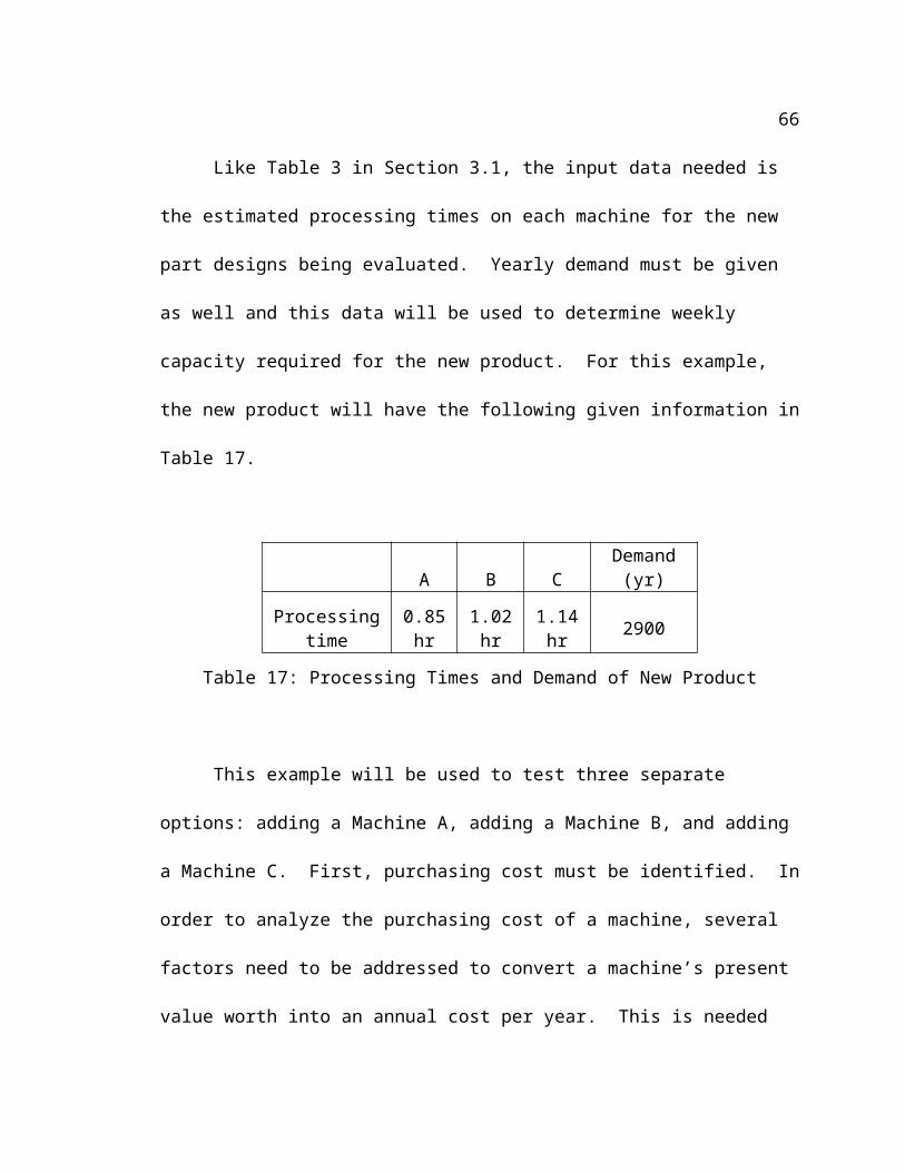
66

6 CONCLUSION

As it has been widely used, ideal cost considers only material costs and labor

costs. As it was shown in the methodology created in this thesis, introducing added

factors in manufacturing such as material handling, purchasing new equipment, and

overtime can provide a more accurate representation of total manufacturing costs.

Incorporating system capacity data into manufacturing cost estimation can allow for more

accurate representation of costs, helping fill the gap between design and manufacturing

departments when implementing new ideas and designs.

6.1 Objective

The objective of the methodology considered in this paper was to further analyze

and consider the effects of system capacity on manufacturing cost estimation. The

purpose of this goal was to eliminate the gap between design and manufacturing

departments which can lead to poor decisions made and ultimately reduce overall costs of

manufacturing.

This methodology incorporated a true cost analysis of multiple designs, with three

implementation options to allow for selecting the minimum manufacturing cost option.

The three implementation alternatives—minimizing material handling costs, route

splitting to minimize overtime costs, and purchasing new machines—all provide an

implementation solution which may provide a cost effective solution. The methodology

can provide actual costs of multiple designs. It is ultimately up to the user which designs

are chosen and with what implementation process. The goal was to provide the user with

the available options and for the user to determine which best suits their needs.

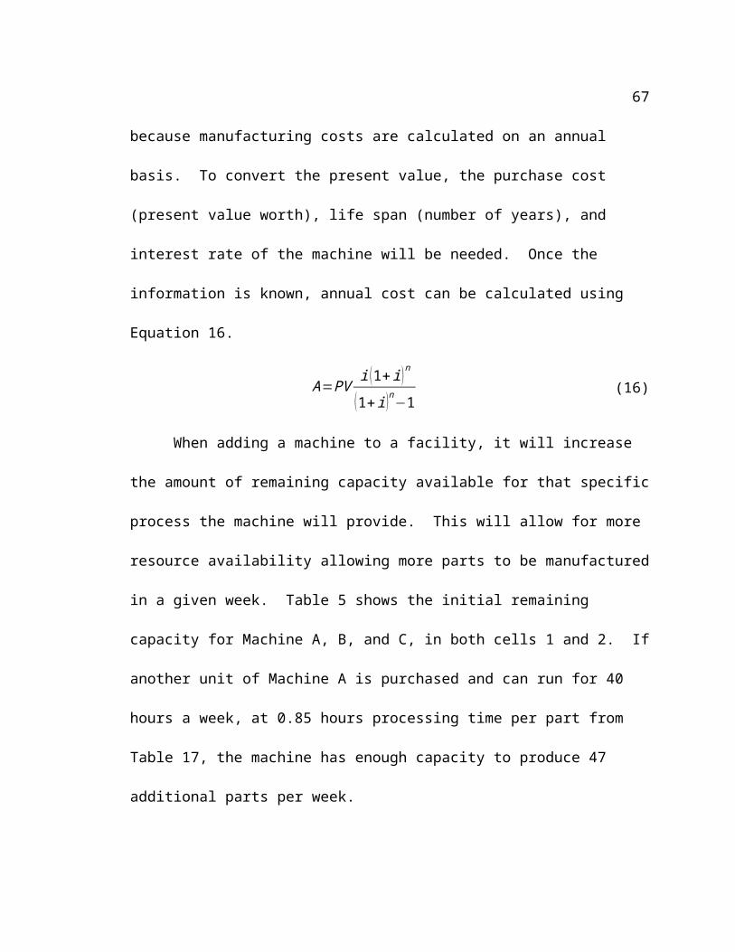
67

By using ideal cost as the input of this methodology, the ideal cost serves as a

foundation of true cost. Using a feature based cost estimator, coupled with the

methodology, one can more accurately provide individualized results based on the

facilities system capacity. The results have shown that ideal cost alone provides an

underestimation of true manufacturing costs. The results from Section 5 show that using

additional manufacturability factors, such as overtime and material handling costs, can

affect true manufacturing costs.

6.2 Benefits

The methodology proposed provides many benefits that can help a manufacturing

company looking to introduce new products into their existing facility. It is not only

important add new clients to a business and to increase business and productivity, but

also to gain a cost benefit from the additional clients.

Many companies will add new customers and business without realizing the new

product being introduced might cost more money to manufacture than originally thought

out. That is why it is important to accurately depict true manufacturing costs prior to

implementation. Once implementation has already begun, costs for engineering and

production changes become much higher. This is why it is important to realize

manufacturing cost estimations during the preliminary design phase.

6.3 Future Work

There are opportunities for future work in this methodology, to develop it into a

complex estimation tool. The main purpose of this methodology was to provide a

method of introducing new products into a facility by means of analyzing manufacturing

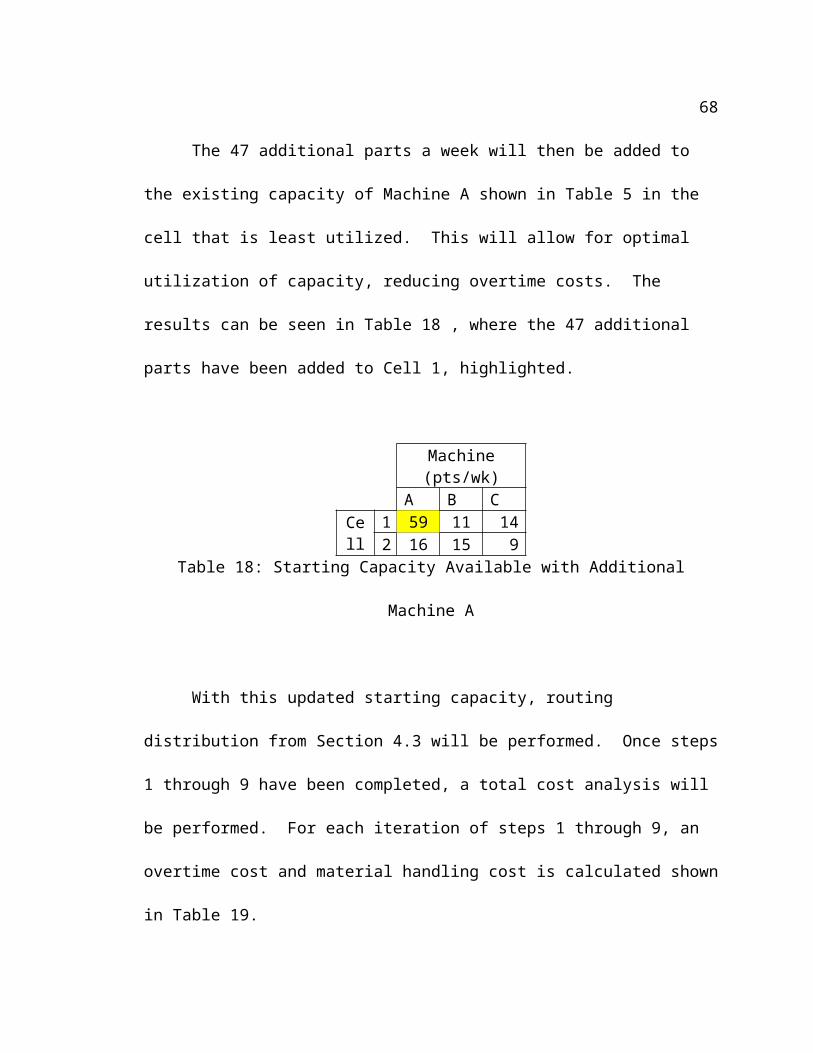
68

costs. This methodology can be adapted to provide use for many different types of

implementation options and estimation calculations.

One suggestion for future work would be to visit more implementation options as

possible solutions. Outsourcing could be another alternative implementation for the

methodology. Outsourcing was not visited in this paper due to its similarity with

overtime costs. As overtime costs are simply a fixed value over a certain time, same goes

with outsourcing. There are other factors in outsourcing such as delivery costs and

scheduling times that would need to be considered.

Another useful alternative which could be looked at further is layout

reconfiguration. It could be beneficial to add an alternative that allows the facility to

rearrange the layout to minimize costs of all products. This posed several issues with

cost estimation is it was difficult to quantify downtime during rearrangement and being

able to assess a cost to that downtime. It also brought another level of complexity to the

methodology that would have made the methodology more complex than what was

necessary. The user would not only have to decide which implementation was better but

also evaluate current needs of existing production requirements and having to make a

decision on whether to put those on hold during reconfiguration.

Along with additional alternatives which can be evaluated, another useful route to

consider is incorporating non-constant demand into the methodology. Being able to

account for non-constant demand is something that can be of great use seeing as constant

demand is only for ideal situations. In the real world, demand is ever changing. To be

able to account for this can be difficult to quantify, and to incorporate in equations. It

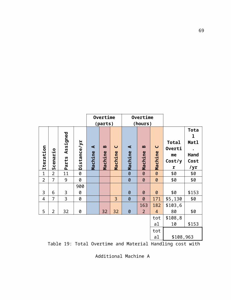
69

would be beneficial to the user to incorporate changing demand to evaluate results to a

more accurate depiction of realistic production values.

70

REFERENCES

[1] B. Baumgart, “A polyhedron representation for Computer Vision,” (1975) AFIPS

Conference Precedings, vol. 44, pp. 589-596.

[2] C. Feng, A. Kusiak, C. Huang, “Cost Evaluation in Design with Form Features,”

Computer-Aided Design, vol. 28, No. 11, pp. 879-885, 1996.

[9] C. Su, T. Sun, C. Wu, and R. Mayer, “An Integrated Form-Feature-Based Design

System for Manufacturing,” Journal of Intelligent Manufacturing, vol. 6, pp. 277-

290, 1995.

[4] D. G. Bramall, K. R. McKay, B.C. Rogers, P. Chapman, W. M. Cheung, and P.G.

Maropoulos,“ Manufacturability Analysis of Early Product Development,”

International Journal of Computer Integrated Manufacturing, vol. 16, no. 7-8, pp.

501-508, 2003.

[5] D. Xue, and Z. Dong, “Developing a Quantitative Intelligent System for

Implementing Concurrent Engineering Design,” Journal of Intelligent

Manufacturing, vol. 5, pp. 251-267, 1994.

[6] F. M. Defersha and M. Chen, “A Comprehensive Mathematical Model for the Design

of Cellular Manufacturing Systems,” International Journal of Production

Economics, vol. 103, pp. 767-783, 2006.

[7] I. Mahdavi, A. Aalaei, M. M. Paydar, and M. Solimanpur, “Designing a Mathematical

Model for Dynamic Cellular Manufacturing Systems Considering Production

Planning and Worker Assignment,” Computers and Mathematics with

Applications, vol. 60, pp. 1014-1025, 2010.

71

[8] J. Y. Jung, “Manufacturing Cost Estimation for Machine Parts Based on

Manufacturing Features,” Journal of Intelligent Manufacturing, vol. 13, pp. 227-

238, 2002.

[9] K. Choi, and H. Cho, “A Cost Based Algorithm for Design of Cellular

Manufacturing Systems,”CKSME International Journal, vol. 12, pp. 181-190,

1998.

[10] K. L. Needy, R. E. Billo, and R. C. Warner, “A Cost Model for the Evaluation of

Alternative Cellular Manufacturing Configurations,” Computers Ind. Enging, vol.

34, pp. 119-134, 1998.

[11] Kusiak, Andrew. Concurrent Engineering: Automation, Tools, and Techniques. New

York: Wiley, 1993. Print.

[12] "manufacturability" BusinessDictionary.com. WebFinance, Inc. July 17, 2011

<http://www.businessdictionary.com/definition/manufacturability.html>.

[13] M. Chen, “A Mathematical Programming Model for System Reconfiguration in a

Dynamic Cellular Manufacturing Environment,” Annals of Operations Research,

vol. 77, pp. 109-128, 1998.

[14] M. Mantyla, “An Introduction to Solid Modeling,” Computer Science Press, Inc.,

Rockville, MD.

[15] M. M. Ghotboddini, M. Rabbani, and H. Rahimian, “A Comprehensive Dynamic

Cell Formation Design: Bender’s Decomposition Approach,” Expert Systems with

Applications, vol. 38, pp. 2478-2488, 2011.

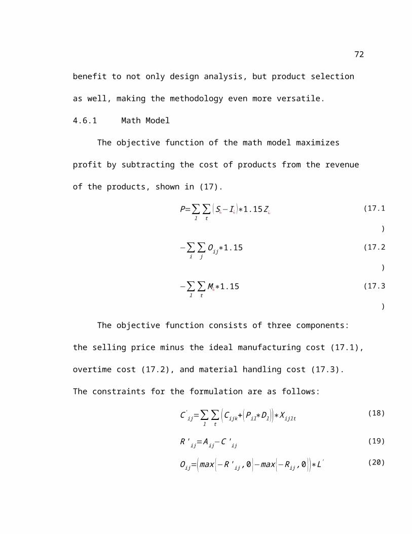
72

[16] S. Ahkioon, A. A. Bulgak, and T. Bektas, “Cellular Manufacturing Systems Design

with Routing Flexibility, Machine Procurement, Production Planning, and

Dynamic System Reconfiguration,” International Journal of Production

Research, vol. 47, No. 6, pp. 1573-1600, 2009.

[17] S. Dowlatshahi, “A Comparison of Approaches to Concurrent Engineering,”

International Journal of Advanced Manufacturing Technology, vol 9, pp. 106-

113, 1994.

[18] Workshop, Design. "DESIGN FOR MANUFACTURABILITY." New Product

Development Solutions. Web. 3 Oct. 2010.

http://www.npd-solutions.com/dfm.html

Documents

Gildenblatt, Robbie 12-17-12