Embed Size (px)
Citation preview

Distributed Computing
What is in the yelp data?Group Project
Hermann Blum, Alexander [email protected], [email protected]
Distributed Computing Group
Computer Engineering and Networks Laboratory
ETH Zurich
Supervisors:
Barbara Keller
Jochen Seidel
Prof. Dr. Roger Wattenhofer
August 18, 2015

Abstract
As a group project we analyzed the data published by yelp for the”Yelp Database Challenge”.Finding clusters in the category-tags, we show how to sort the busi-nesses in a hierarchical order. On this basis, we visualize the geograph-ical distribution of different categories, finding hotspots like ”china-town”.Using Machine Learning Algorithms, we are able to predict whethera business of a given subcategory will attract more or less customersin a given location. This enables us to mark good locations to open abusiness of a given category.
Contents
1 General Statistics about the given data 21.1 Businesses . . . . . . . . . . . . . . . . . . . . . . . . . . . . . 21.2 Reviews . . . . . . . . . . . . . . . . . . . . . . . . . . . . . . 3
2 Making the Data More Useful 32.1 Super Categories . . . . . . . . . . . . . . . . . . . . . . . . . 32.2 Sub Categories . . . . . . . . . . . . . . . . . . . . . . . . . . 52.3 Finding Neighbours to Businesses . . . . . . . . . . . . . . . . 52.4 User Reviews . . . . . . . . . . . . . . . . . . . . . . . . . . . 52.5 Statistics of the Categories . . . . . . . . . . . . . . . . . . . 62.6 Distribution of Businesses in a City . . . . . . . . . . . . . . . 9
3 Visualizing Data 9
4 Predicting a Good Location 104.1 Goal . . . . . . . . . . . . . . . . . . . . . . . . . . . . . . . . 104.2 What is a ”Good” Location? . . . . . . . . . . . . . . . . . . 104.3 Finding a Correlation . . . . . . . . . . . . . . . . . . . . . . 114.4 Support Vector Machines . . . . . . . . . . . . . . . . . . . . 124.5 Random Forests . . . . . . . . . . . . . . . . . . . . . . . . . 124.6 Seleting Features . . . . . . . . . . . . . . . . . . . . . . . . . 134.7 Redefine ”good” Location . . . . . . . . . . . . . . . . . . . . 134.8 Training the Machine . . . . . . . . . . . . . . . . . . . . . . . 144.9 Cross Validation . . . . . . . . . . . . . . . . . . . . . . . . . 144.10 Performance . . . . . . . . . . . . . . . . . . . . . . . . . . . . 144.11 Visualizing the Prediction . . . . . . . . . . . . . . . . . . . . 15
1
5 Conclusion 15
1 General Statistics about the given data
1.1 Businesses
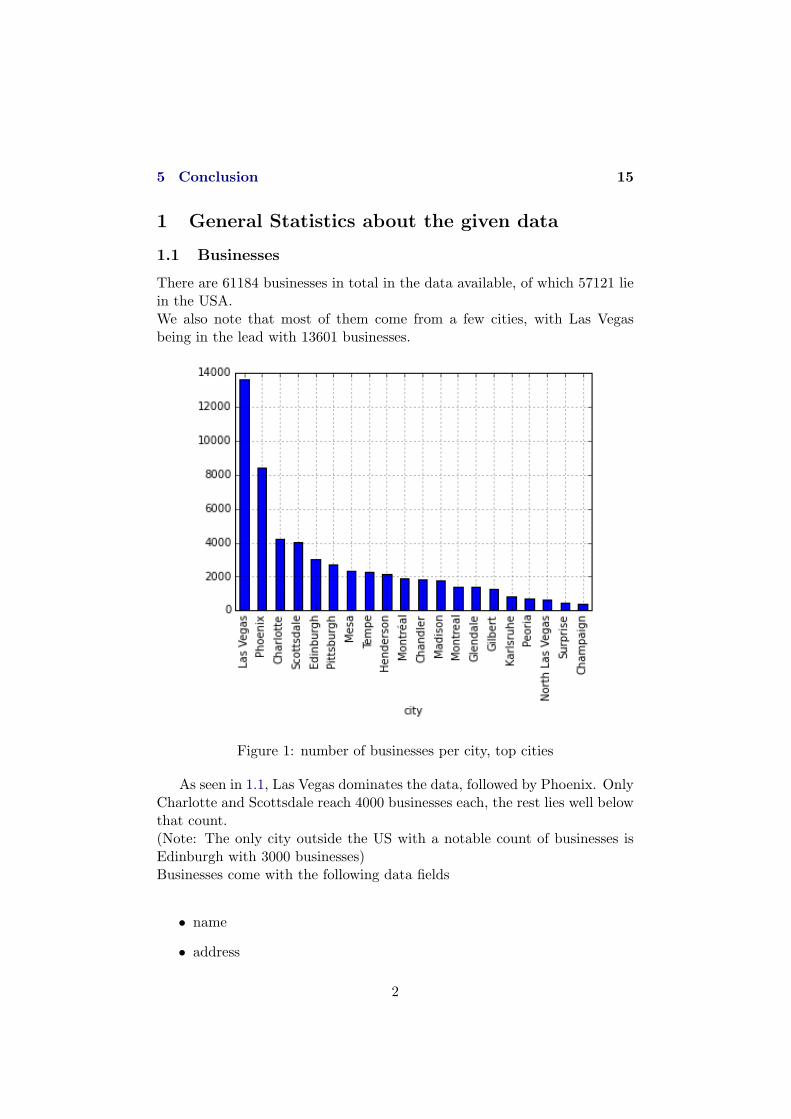
There are 61184 businesses in total in the data available, of which 57121 liein the USA.We also note that most of them come from a few cities, with Las Vegasbeing in the lead with 13601 businesses.
Figure 1: number of businesses per city, top cities
As seen in 1.1, Las Vegas dominates the data, followed by Phoenix. OnlyCharlotte and Scottsdale reach 4000 businesses each, the rest lies well belowthat count.(Note: The only city outside the US with a notable count of businesses isEdinburgh with 3000 businesses)Businesses come with the following data fields
• name
• address
2
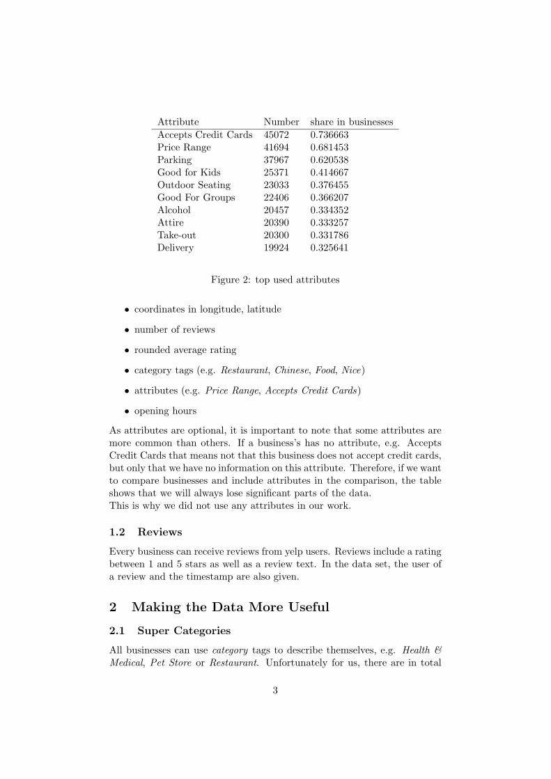
Attribute Number share in businessesAccepts Credit Cards 45072 0.736663Price Range 41694 0.681453Parking 37967 0.620538Good for Kids 25371 0.414667Outdoor Seating 23033 0.376455Good For Groups 22406 0.366207Alcohol 20457 0.334352Attire 20390 0.333257Take-out 20300 0.331786Delivery 19924 0.325641
Figure 2: top used attributes
• coordinates in longitude, latitude
• number of reviews
• rounded average rating
• category tags (e.g. Restaurant, Chinese, Food, Nice)
• attributes (e.g. Price Range, Accepts Credit Cards)
• opening hours
As attributes are optional, it is important to note that some attributes aremore common than others. If a business’s has no attribute, e.g. AcceptsCredit Cards that means not that this business does not accept credit cards,but only that we have no information on this attribute. Therefore, if we wantto compare businesses and include attributes in the comparison, the tableshows that we will always lose significant parts of the data.This is why we did not use any attributes in our work.
1.2 Reviews
Every business can receive reviews from yelp users. Reviews include a ratingbetween 1 and 5 stars as well as a review text. In the data set, the user ofa review and the timestamp are also given.
2 Making the Data More Useful
2.1 Super Categories
All businesses can use category tags to describe themselves, e.g. Health &Medical, Pet Store or Restaurant. Unfortunately for us, there are in total
3
nearly 800 different tags.We aimed to reduce the number of categories by grouping them together insome way. To achieve this, we first created a graph of all existing categorytags in the following fashion:
1. Create a node for every single category tag
2. Connect the tags which are mentioned together
3. To improve precision, introduce a weight to every edge. As a weightwe chose how often two labels are mentioned together.
Luckily this is easily achieved with pandas and networkx in python. We usedpandas to expand the category tags and count pairwise cooccurence. Theresulting matrix could then easily be exported to networkx as an adjacencymatrix to create the graph.We now have a graph with nearly 800 nodes and many more connections.To continue we base or work around graph modularity and community de-tection. Luckily there is a nice implementation of the Louvain method ofpartitioning in python which works together with networkx.This algorithm detected ten communities (or super categories) in our graph(with a modularity between 0.6 and 0.7). In order to make them more hu-man understandable we assigned labels to the super categories. Since thiswas for informational purpose only, we just took the label in every commu-nity which appeared most often. This lead to the following categories:
• Restaurants
• Shopping
• Food
• Active Life
• Health & Medical
• Home Services
• Automotive
• Event Planning & Services
• Pets
• Beauty & Spas
4

2.2 Sub Categories
In the next step we aim to improve classification by making it more detailed- partitioning every super category we found above in several sub categories.Directly using the Louvain algorithm again unfortunately gives no good re-sults since the nodes are tied too closely together by some nodes which areconnected to everything, e.g. the node Restaurant in the super categorywith the same name.We use a simple solution to solve this problem: We remove this node. With-out the part that connects everything, the Louvain algorithm is successfulagain and returns several sub categories per super category.Because of just ripping out the most popular node in some super categorieswe are left with single nodes that are not connected to anything and thusbecome their own subcategory. Those categories sometimes just contain onebusiness. Since it doesnt make a lot of sense to categorize just one thing,we collect all those leftover sub categories and simply declare them as un-categorized.
2.3 Finding Neighbours to Businesses
For every business its coordinates in longitude and latitude are given. Anessential part of our data analysis includes the relation between businessesand their neighbours.To find neighbours of a business efficiently, we define a grid over the worldmap and sort the businesses into this grid.One can now start with the grid cell of a given business and find neigh-bours by calculating only the distances to businesses in adjacent cells, withincreasing radius. In the end, one only has to filter out all businesses notlaying in the incircle of this cell cluster.
Distances between coordinates are usually calculated using the Formulaof Vincenty, which describes the distance between two points on the surfaceof a spheroid. A profiling showed that this calculation is the bottleneckof performance, so we switched to the slightly less precise1 assumption ofmodeling the earth as a sphere.
2.4 User Reviews
An important function of yelp are user reviews. Users can rate a businessbetween 1 and 5 stars and write a text review. Yelp uses the mean of review
1The error of the Haversine function for distances on the surface of a sphere does notexceed 5% with respect to the distance calculated with the function of Vincenty.
5

Figure 3: visualization of the neighbour-finding-algorithm
ratings as an important feature for the search ranking. We analyzed thedistribution of user reviews over time and given stars. Our main results are:
• The number of reviews written on yelp per day is increasing exponen-tially (at least the data published by yelp wants us to believe this)
• distributed over the year, there are more reviews on a summer daythan on a winter day
• with every change of year, one can recognize a steep increase of dailyreviews. This might be linked to the peak of smartphone and computersales in the christmas time.
We next followed the idea that reviews might show trends. For example,the chef of a restaurant could change and this might influence customersatisfaction. However, analyzing trends would require a minimum numberof reviews per time. In the published data, only 12% of the businesses havemore than 50 reviews. As reviews in general differ for a given businessbetween 1 and 5, we had to create a more steady function mapping a datet to the average review in the interval [t − δ, t + δ] for a given δ and thensearched for great changes in this function. Unfortunately this lead not toa satisfactory solution. Our Algorithms either detected a trend for the firstpossible date δ or they detected no trend at all.
2.5 Statistics of the Categories
In a next step, we analyzed the user reviews over the above described dif-ferent categories.
6

Figure 4: reviews per day
Figure 5: the flattend rating history of the 3 restaurants with most reviews,over days in past
7

Figure 6: reviews per category, circles are sized by number of businesses ina subcategory
Category Average User RatingActive Life/Religious Organizations 4.473689Beauty & Spas/Tattoo 4.449621Event Planning & Services/Party & Event Planning 4.336023Event Planning & Services/Uncategorized 4.333333Active Life/Fitness & Instruction 4.255133Beauty & Spas/Dentists 4.236437Automotive/Auto Glass Services 4.194066Pets/Pet Services 4.152262Food/Specialty Food 4.109462Active Life/Uncategorized 4.057366
Figure 7: top rated categories
The analysis of the user ratings (figure 2.5) shows that people are usuallycritical with Restaurants and especially uncritical when it comes to religiousorganizations and tattoo studios. This, of course, can not be generalized asmost of the businesses analyzed are located in the USA.
8

2.6 Distribution of Businesses in a City
Given the number of businesses in the dataset, the biggest cities are LasVegas (US) and Phoenix (US). We also analyzed Edinburgh, which is thebiggest non-US city in the dataset.
City Number of Businesses in DatasetLas Vegas 13601Phoenix 8410Charlotte 4224Scottsdale 4039Edinburgh 3031Pittsburgh 2724Mesa 2347Tempe 2258Henderson 2130Montreal 1870
Figure 8: biggest cities in dataset
On basis of our cell grid which we build for the neighbour search, wecould also analyze the density of businesses in general, different categoriesor features like user ratings and review counts in every cell. Compared overa whole city we can therefore, without knowledge of any kind of map, markthe hotspots of this city.
3 Visualizing Data
To visualize data, we usually used pyplot, a popular library for python tocreate graphics. However, we searched for a way to visualize the geographicdistribution of the businesses and their characteristics. We found GoogleEarth, which has the possibility to add custom geometries and locationsusing the KML file format, a standard for map services.Now just marking all the businesses with respect to their subcategory doesnot work well, as seen in figure 3
Do get a better overview, we used the cell object already used to findneighbours and visualized these cells on the map. Given the businesses ina cell, one can simply define a function that maps a list of businesses to avalue. This can be just the number of businesses but also the average reviewand various other metrics.Each cell becomes a rectangle on the map, filled with a color by a giventransparency. To view distributions over a map, we found two good work-ing methods:
9

Figure 9: markers for all businesses, coloured by subcategory around theLas Vegas Boulevard
• greyscale with 0 transparency is usually the best way to find clusters
• constant colors with by the value of the cell varying transparency worksgood to compare different distributions, but only real hot spots becomevisible
4 Predicting a Good Location
4.1 Goal
One of the big questions we analyzed was: Has the neighbourhood of abusiness influence on the user ratings for this business? The idea behindthis is that a disco might be better located in the near of hotels and barsthan next to an automotive shop.
4.2 What is a ”Good” Location?
Our first challenge was to define the factors describing a good location. Thisis difficult in several aspects: You do not only need to have an idea whatmakes a business good, but also need to express this with some kind of met-ric to be able to compare it.Our naive first approach was to define a good location by the average userrating: If youre opening a business, you sure aim to make people like it -are there factors that make it easier to get a higher rating? Additionally
10
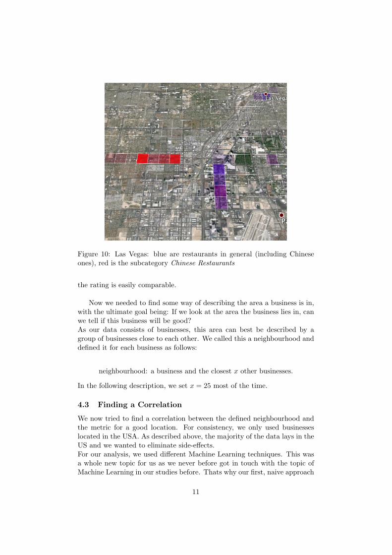
Figure 10: Las Vegas: blue are restaurants in general (including Chineseones), red is the subcategory Chinese Restaurants
the rating is easily comparable.
Now we needed to find some way of describing the area a business is in,with the ultimate goal being: If we look at the area the business lies in, canwe tell if this business will be good?As our data consists of businesses, this area can best be described by agroup of businesses close to each other. We called this a neighbourhood anddefined it for each business as follows:
neighbourhood: a business and the closest x other businesses.
In the following description, we set x = 25 most of the time.
4.3 Finding a Correlation
We now tried to find a correlation between the defined neighbourhood andthe metric for a good location. For consistency, we only used businesseslocated in the USA. As described above, the majority of the data lays in theUS and we wanted to eliminate side-effects.For our analysis, we used different Machine Learning techniques. This wasa whole new topic for us as we never before got in touch with the topic ofMachine Learning in our studies before. Thats why our first, naive approach
11

was a linear regressor on the linear metric of average stars.We later changed the problem by switching the metric for a ”good” locationfrom a linear range of stars to classes (e.g. good business, bad business),turning the regression problem into a problem of classification. Our maintool in this context were Support Vector Machines. They had, compared toother algorithms, the best results. However, Random Forests were a reallyhelpful tool as they worked significantly faster and provide info on how im-portant each feature is for deciding.For all machine learning tasks we used the python library scikit-learn whichproved to be an easy to use and powerful tool.
4.4 Support Vector Machines
A support vector machine (SVM) aims to find separation lines between thedata classes. Of course data can often not be linearly separated, but byusing certain kernels the data can be transformed in a way that makes alinear separation possible in the transformed data while the separation linecan take different shapes in the original data.Scikit learn offers three different kinds of kernels:2
Linear Not transforming the data
Polynomial Using a polynomial of degree n
RBF Using a radial base function in the form of exp(−γr2) with a param-eter γ and r as the distance from a point x
4.5 Random Forests
Random forests use a specified number of decision trees which grow inde-pendently from each other and are generated randomly. Each tree is randomin two ways: Each tree is trained with a random choice from the trainingdata set, and each decision in the trees is based on a random subset of thefeatures.When predicting each tree makes it’s own decision and the ultimate decisionwill be the what most of the trees decide.A nice thing about random forests is that they proved to be much fasterthan the SVM since the training and classification can be parallelised effi-ciently. (Although it later turned out that the results were a little worsecompared to the slower SVM with RBF kernel). This was helpful for usduring development, as we could quickly check, if an added feature could
2More info here: http://scikit-learn.org/stable/modules/svm.html#kernel-functions
12
influence the prediction.Moreover, Random Forests weight the different features. We could use thisweight as a feedback how relevant the added features were.
4.6 Seleting Features
Given the set of businesses we will now call a neighbourhood, one can de-scribe this set calculating different measurable features:
1. Obvious features are the mean, variance, minimum and maximum ofthe review counts and average ratings of the businesses in one set. Toassure that the data is comparable, we only counted the reviews overone year.
2. As the geographic density of businesses varies, we took into accountthe area over which the set of 25 nearest neighbours is distributed,described by both radius and area.
3. Recalling the idea that a disco might work better in the near of a barthan in the near of an automotive store, the categories of the neigh-bours are important. We therefore counted the number of occurrencesof super categories and subcategories in each neighbourhood.
4. As the selection of x nearest businesses as neighbours is slightly ar-bitrary, next to the mean over x businesses we weighted the reviewcounts by distance and added them into an additional feature.
4.7 Redefine ”good” Location
Unfortunately, we could not find any correlation between the neighbourhoodof a business and its average rating.We tried several approaches, as mentioned above:
1. Regression as well as classification (both five classes, one each per star,as well as two classes good and bad, containing the upper and lower50 percent)
2. Different classification schemes: SVM with different kernels, Randomforests
None of those approaches was successful, we never got a better result thanjust guessing a constant (e.g. the mean value of stars or a random class).We therefore went back to the problem of defining a metric for a good loca-tion. It occurred to us that not only the rating of customers is an importantmetric for a business owner, but also the number of customers reachableat a certain location. As the checkin function in yelp is not used by a lot
13

of people, the best metric for the number of people reachable at a certainlocation in the data set is the number of reviews.Unfortunately, the absolute number of reviews is not really helpful, sincesome businesses have been on yelp for many years while others are only afew years old. Therefore we only look at the number of reviews over a fixedinterval of time. As the number of reviews per day varies over the year (seefigure 2.4), we defined our new metric for a good location as the number ofreviews over the last year, ending with the newest review.
4.8 Training the Machine
We now have for every business on the one hand a neighbourhood with cer-tain features and on the other hand the classification based on last yearsreviews. We train our machine per subcategory, e.g. for Restaurants/Chi-nese and Local Services/Plumbers.
4.9 Cross Validation
To avoid overfitting scikit-learn has already implemented cross-validationfeatures which are easy to use. We used 80% of the data for training and20% for testing.The method we used in scikit-learn was a stratified shuffle split Which ran-domly selects the training and test data, but ensures that the classes appearin the same distribution as in the original data (so if good/bad is 50/50, inthe training and test data they will also be 50/50). This process is repeated5 times and the precision (as measured with the test data) is averaged.
4.10 Performance
We achieve a performance of up to 70% accuracy. Unfortunately, not allcategories can be predicted very well. Some categories can not really bepredicted and still are not better than 50%.This is not an ideal result, but at least for some categories we are muchbetter than just randomly guessing.We also note that the performance varies by city: In Las Vegas we can pre-dict with high accuracy where to place Chinese or American Restaurantswhile in Phoenix we can predict better where to put transportation servicesor Bars/Clubs.
We can also use the random forests to get insight which features are im-portant for the decision process. The most important features are: location,lifetime on yelp and average number of reviews in the neighbourhood.
14

Subcategory Prediction AccuracyRestaurants/Chinese 67%Restaurants/American (Traditional) 67%Event Planning & Services/Transportation 66%Pets/Pet Stores 66%Event Planning & Services/Public Services & Government 66%
Figure 11: subcategories with highest prediction accuracy in Las Vegas
Subcategory Prediction AccuracyEvent Planning & Services/Transportation 66%Beauty & Spas/Tanning 66%Home Services/Printing Services 62%Restaurants/Nightlife 60%Restaurants/Fast Food 60%
Figure 12: subcategories with highest prediction accuracy in Phoenix
4.11 Visualizing the Prediction
Here we visualize the results: The red areas show the predictions to place atanning studio in that cell, the blue ones show the prediction for businessesin the subcategory nightlife.The brighter the color the more recommended is the spot.We can see in figure 4.11 that while tanning studious kind of work every-where, nightlife is concentrated around a few hot spots downtown and in anindustrial area (where it is possibly ok to be loud)
5 Conclusion
We were able to group the data into meaningful super and sub categories,enabling us to further analysis and visualize the businesses. We were ableto find hot spots of businesses of a certain kind (e.g. china town) as well asidentify general hotspots (e.g. the las vegas boulevard or simply big malls).We further could use this methods to train a machine learning algorithm todetect neighbourhoods which are well suited for a certain type of business.
15

Figure 13: prediction of good locations for Nightlife (blue) and TanningStudious (red)
16