Embed Size (px)
Citation preview
DIPLOMARBEIT
Halbeinfache Frobenius-Mannigfaltigkeiten
und Quantenkohomologie
(Semisimple Frobenius Manifoldsand Quantum Cohomology)
angefertigt am Mathematischen Institut
vorgelegt der
Mathematisch-Naturwissenschaftlichen Fakultat derRheinischen Friedrich-Wilhelms-Universitat Bonn
Von
Arend Bayer
aus Tubingen
September 2003

2

CONTENTS 3
Contents
1 Introduction: Semisimple Frobenius manifolds 5
1.1 Plan of the paper . . . . . . . . . . . . . . . . . . . . . . . . . . . 5
1.2 Acknowledgements . . . . . . . . . . . . . . . . . . . . . . . . . . 6
2 Deutsche Zusammenfassung 7
3 Definitions and Notations 11
3.1 Frobenius Manifolds . . . . . . . . . . . . . . . . . . . . . . . . . 11
3.2 Quantum Cohomology . . . . . . . . . . . . . . . . . . . . . . . . 12
4 Semisimple Computations 15
4.1 Fano manifolds with minimal (p, p)-cohomology . . . . . . . . . . 15
4.2 Fano threefolds with minimal cohomology . . . . . . . . . . . . . 17
4.2.1 Notation . . . . . . . . . . . . . . . . . . . . . . . . . . . . 17
4.2.2 Tables of correlators . . . . . . . . . . . . . . . . . . . . . 17
4.2.3 Canonical coordinates . . . . . . . . . . . . . . . . . . . . 18
4.2.4 Multiplication tables, idempotents, and metric coefficients 18
5 Dubrovin’s Monodromy data 23
5.1 The first structure connection . . . . . . . . . . . . . . . . . . . . 23
5.2 Stokes matrices of an irregular singular point of a differentialequation . . . . . . . . . . . . . . . . . . . . . . . . . . . . . . . . 23
5.3 Stokes matrices of a Frobenius manifold . . . . . . . . . . . . . . 34
5.4 Dubrovin’s monodromy data . . . . . . . . . . . . . . . . . . . . 36
6 Exceptional systems and Dubrovin’s conjecture 39
6.1 Exceptional systems in triangulated categories . . . . . . . . . . 39
6.2 Dubrovin’s conjecture . . . . . . . . . . . . . . . . . . . . . . . . 40
7 Semisimple mirror symmetries 41
7.1 The mirror construction . . . . . . . . . . . . . . . . . . . . . . . 41
7.2 The Milnor fibration . . . . . . . . . . . . . . . . . . . . . . . . . 42
7.2.1 A homology bundle . . . . . . . . . . . . . . . . . . . . . 42
7.2.2 Lefschetz thimbles . . . . . . . . . . . . . . . . . . . . . . 42
7.2.3 Seifert matrix . . . . . . . . . . . . . . . . . . . . . . . . . 44
7.3 The twisted de Rham-complex . . . . . . . . . . . . . . . . . . . 45
7.4 Frobenius manifold mirror symmetry . . . . . . . . . . . . . . . . 46
7.5 Relating Stokes and Seifert matrix . . . . . . . . . . . . . . . . . 47
7.6 Homological mirror symmetry and exceptional systems . . . . . . 49
7.7 Putting it together . . . . . . . . . . . . . . . . . . . . . . . . . . 50
8 Blow-ups 51
8.1 Complete exceptional system and blow-ups . . . . . . . . . . . . 51
8.2 Semisimplicity and blow-ups . . . . . . . . . . . . . . . . . . . . . 51
8.2.1 Gathmann’s results . . . . . . . . . . . . . . . . . . . . . . 52
8.2.2 Proof of Theorem 8.2.1 . . . . . . . . . . . . . . . . . . . 55

4 CONTENTS
8.3 Further Questions . . . . . . . . . . . . . . . . . . . . . . . . . . 59
References 61

5
1 Introduction: Semisimple Frobenius manifolds
In his talk at the ICM in Berlin 1998, Dubrovin proposed a surprising conjectureanswering the question which Fano manifolds could have generically semisimplequantum cohomology. This diploma thesis
• explains this conjecture,
• relates it to mirror symmetry conjectures,
• gives several computations on manifolds that do have semisimple quantumcohomology, and
• proves (a part of) Dubrovin’s conjecture for a large class of manifolds.
A Frobenius manifold is a complex manifold M equipped with a multipli-cation on the tangent bundle TM and a flat metric that satisfy a numberof axioms. In general, one needs infinitely many numbers to describe a sin-gle Frobenius manifold. However, for those Frobenius manifolds that have asemisimple point x (i. e., (TxM, ) is isomorphic as an algebra to Cn), thereexist two independent classifications. Both classifications identify the germ ofsuch a Frobenius manifold by a finite number of characteristic numbers. Inother words, semisimple Frobenius manifolds are easier to understand.
1.1 Plan of the paper
In section 3, we recall the basic definitions and notations of Frobenius manifoldsand quantum cohomology from [Man99].
Section 4 gives examples of computations of semisimple quantum cohomol-ogy. We compute the special coordinates (the classifying data in Yu. I. Manin’sclassification of semisimple Frobenius manifolds) of three families of Fano three-folds with minimal cohomology.
Section 5 gives a detailed definition of Dubrovin’s monodromy data (thatclassifies semisimple Frobenius manifolds). We devote particular care to theconstruction of Stokes matrices; here we follow [vdPS03], partly rephrasing itin a more abstract language.
In the following section 6, we discuss exceptional systems in triangulatedcategories, and give the exact statements of Dubrovin’s conjecture.
Section 7 is devoted to the bigger conjectural picture underlying Dubrovin’sconjecture. This involves the homological mirror conjecture in its assumedform for semisimple quantum cohomology and total spaces of unfoldings ofhypersurface singularities (7.6), the corresponding numerical mirror symmetryconjecture as an isomorphism of Frobenius manifolds (as in 7.4.1), and theexplanation of Stokes matrices in the case of unfoldings of singularities. Partsof this section are directly inspired by the paper [HIV00] by the physicists Hori,Iqbal and Vafa.
Finally, in section 8, we prove the theorem 8.2.1. Its statement can beformulated concisely (and almost correctly) as: If we know that Dubrovin’sconjecture is true for X, then it is true for its blow-up X at a point. The idea

6 1 INTRODUCTION: SEMISIMPLE FROBENIUS MANIFOLDS
to the proof is similar to the case of Del Pezzo-surfaces, which was treated in[BM01].
1.2 Acknowledgements
I would like to thank Gunther Vogel for comprehensive proof-reading and mybrother Tilman Bayer for useful remarks clarifying the exposition; BarbaraFantechi for suggestions related to footnote 10. Several discussions with ClausHertling substantially helped my understanding of section 7. Finally, I amindebted to my advisor Yuri I. Manin for continued inspiring and encouragingsupport.

7
2 Deutsche Zusammenfassung
Einfuhrung. Frobenius-Mannigfaltigkeiten wurden 1990 von Boris Dubrovinals Axiomatisierung (eines Teils) der mathematischen Struktur topologischerFeldtheorien eingefuhrt. Eine Frobenius-Mannigfaltigkeit ist im Wesentlicheneine flache Mannigfaltigkeit mit Metrik und einer Produkstruktur auf dem Tan-gentialbundel, die bestimmte Axiome erfullen (cf. Definition 3.1.1 fur Details).Das wichtigste Axiom ist eine Integrabilitatsbedingung, die die Struktur einerFrobenius-Mannigfaltigkeit erstaunlich starr macht.
Die bekannteste Beispielklasse von Frobenius-Mannigfaltigkeiten entstehtaus der Quantenkohomologie einer glatten projektiven Varietat V . In diesemFall ist die Mannigfaltigkeit einfach der Vektorraum H ∗(V,C). Die Metrikist gegeben durch die Poincare-Paarung. Eine Multiplikation auf dem Tan-gentialbundel dieser Mannigfaltigkeit bedeutet das Folgende: an jedem Punktx ∈ H∗(V,C) ist der Tangentialraum an x naturlich identisch zu H ∗(V,C).Ein Produkt auf Tx ist also ein Produkt auf der Kohomologie, das abervon x als Parameter abhangt. Das Produkt ist definiert durch das Gromov-Witten-Potential, eine erzeugende Funktion aus sogenannten Gromov-Witten-Invarianten; siehe Definition 3.2.2 und Satz 3.2.3. Dass das hierdurch definierteQuantenprodukt assoziativ ist, ist eine sehr uberraschende und tiefe Aussage.Man kann es verstehen als deformiertes Cup-Produkt.
Diese Diplomarbeit beschaftigt sich mit solchen Frobenius-Mannigfaltig-keiten M, bei denen fur generisches m ∈ M die Algebrastruktur auf TmMzerfallt, d. h. dass TmM als Algebra isomorph zu Cn mit komponentenwei-ser Multiplikation ist. Halbeinfache Frobenius-Mannigfaltikeiten sind aus ver-schiedenen Grunden einfacher zu verstehen. Ein Grund ist, dass die multiplika-tive Struktur auch in einer Umgebung von m sehr einfach zerfallt, siehe Propo-sition 3.1.4. Weiterhin sind Keime solcher Mannigfaltigkeiten vergleichsweiseleicht zu klassifizieren.
Spezielle Koordinaten. Ein sehr einfach zu definierendes Klassikations-datum sind die sog. speziellen Koordinaten. Sie wurden von Yuri I. Manineingefuhrt und sind in gegeben Fallen auch einfach zu berechnen.
Dies wird in Kapitel an drei Familien dreidimensionaler Fano-Mannigfaltig-keiten durchgefuhrt. Diese Familien zeichnen sich dadurch aus, dass ihre Koho-mologie nur vierdimensional ist, die minimal mogliche Dimension. Von Bon-dal, Kuznetsov und Orlov wurden fur diese Falle jeweils einzelne Gromov-Witten-Invarianten berechnet. Mithilfe der Relationen, die sich aus der As-soziativitat der Produktstruktur der zugehorigen Frobenius-Mannigfaltigkeitenergeben, lassen sich dann weitere Invarianten rein algebraisch berechnen.
Fur die Produktstruktur berechnen wir hier explizit die Zerlegung als Alge-bra in C4 durch Angabe der vier Idempotenten. Und zwar fur den Fall, dass deroben mit x ∈ H∗(V ) bezeichnete Parameter im Unterraum H2(V ) liegt, bzw.in dessen erster infinitesimaler Umgebung. Daraus lassen sich die speziellenKoordinaten berechnen.
8 2 DEUTSCHE ZUSAMMENFASSUNG
Stokes-Matrizen. Von Dubrovin stammt die Konstruktion eines flachenZusammenhangs auf P1 ×M fur jede Frobenius-Mannigfaltigkeit M, der aucherster Strukturzusammenhang der Frobenius-Mannigfaltigkeit genannt wird;cf. Definition 5.1.1. Dieser Zusammenhang hat einen Pol zweiter Ordnungentlang 0 × M. Solche Zusammenhange lassen sich nun wiederum klas-sifizieren, und das wesentliche Datum dabei sind die sogenannten Stokes-Matrizen. Zur ihrer Definition ist einiges an Theorie der Differential-Modulnuber dem Differential-Ring C(z) der Keime komplexer Funktionen (mitDerivation ∂
∂z ) notig; eine entscheidende Technik ist dabei die Verwendung vonFunktionen mit asymptotischer Entwicklung nahe 0 in einem Sektor in C. DieseTheorie wird im Kapitel 5 uberblicksartig vorgestellt, die Darstellung folgt (mitAnderungen) der in [vdPS03].
Gemaß Dubrovin wird erklart, wie sich diese auf den ersten Strukturzusam-menhang anwenden lasst.
Dubrovins Vermutung und halbeinfache Spiegelsymmetrie. Das dar-auffolgende Kapitel berichtet uber eine Vermutung von Dubrovin, die besagt,bei genau welchen Varietaten V halbeinfache Quantenkohomologie zu erwartenist. Und zwar sei dies genau fur diejenigen der Fall, fur die die derivierte Kate-gorie Db(V ) der koharenten Garben auf V in einem gewissen Sinne halbeinfachist; genauer gesagt, falls es in Db(V ) ein sogenanntes exzeptionelles System vonObjekten gibt, siehe Definition 6.1.1.
Ferner vermutet Dubrovin, dass sich in diesem Fall auch die Stokes-Matrixder Frobenius-Mannigfaltigkeit zu V aus der halbeinfachen Struktur von Db(V )ablesen lasst. Das Kapitel 7 versucht zu erklaren, warum dies aus dem Kontextder Spiegelsymmetrie zu V zu erwarten ist:
Zu einer solchen Varietat V ist der Spiegelpartner eine affine VarietatY mit einer gegebenen Funktion f auf Y mit isolierten Singularitaten. Ausden Deformationen dieser Funktion f , die Entfaltungen der Singularitatenliefern, entsteht eine Frobenius-Mannigfaltigkeit. Spiegelsymmetrie wurde be-sagen, dass diese Frobenius-Mannigfaltigkeit isomorph zu der der Quantenko-homologie von V ist; im Fall von Pn ist dies von Barannikov bewiesen wurden(cf. Satz 7.4.1). Wir versuchen zu zeigen (ohne vollstandigen Beweis), dass dieStokes-Matrix dieser Frobenius-Mannigfaltigkeit identisch zu der rein topolo-gisch aus der Milnor-Faserung von f definierten Seifert-Matrix ist.
Daraus, und aus einer weiteren Spiegelsymmetrievermutung analog zu Kont-sevichs homologischer Spiegelsymmetrie, wurde Dubrovins Behauptung uberStokes-Matrizen folgen.
Aufblasungen. Das eigentlich neue Resultat dieser Arbeit ist Satz 8.2.1.
Es sei X eine n-dimensionale projektive Varietat, und X die Aufblasungvon X an einem Punkt x ∈ X; sei E ⊂ X der exzeptionelle Divisor (Faser uberx) der Abbildung X → X, mit demselben Buchstaben bezeichnen wir auch diezugehorige Kohomologieklasse in H2(X). Es ist H∗(X) ∼= H∗(X) ⊕ C · E ⊕C · E2 ⊕ . . .C · En−1, und damit ist auch das Cup-Produkt in H∗(X) (fast)vollstandig beschrieben.
9
Fur das deformierte Cup-Produkt der Quantenkohomologie stellt sich nunfolgende Frage:
Wenn die Frobenius-Mannigfaltigkeit der Quantenkohomologie vonX halbeinfach ist, gilt dann dasselbe auch fur X?
Falls namlich die Halbeinfachheit fur X gilt, musste gemaß Dubrovins Vermu-tung Db(X) ein exzeptionelles System haben. Dasselbe gilt dann nach einemResultat von Bondal auch fur die Kategorie Db(X). Folglich musste auch Xhalbeinfache Quantenkohomologie haben.
Damit ist obige Frage ein ernsthafter Test fur Dubrovins Vermutung. Unterzwei technischen Zusatzvoraussetzungen beantwortet unser Satz diese Fragepositiv. Der Beweis beruht wesentlich auf Resultaten von Gathmann, die dieGromov-Witten-Invarianten von X und X in Beziehung setzen. Ein Verschwin-dungssatz von ihm ermoglicht eine partielle Kompaktifizierung des Parameter-raums, fur den das Quantenprodukt definiert ist. Entlang des neu hinzugefugtenDivisors zerfallt das Quantenprodukt von X in die direkte Summe eines halb-einfachen Anteils und eines Anteils isomorph zum Quantenprodukt von X.

10 2 DEUTSCHE ZUSAMMENFASSUNG
11
3 Definitions and Notations
3.1 Frobenius Manifolds
To fix definitions and notations, we collect here the relevant definitions from[Man99].
Definition 3.1.1. A Frobenius manifold with flat identity is a complex mani-fold Mn endowed with the following structures on the tangent sheaf TM:
• A non-degenerate symmetric bilinear form g : TM⊗ TM → OM, calledthe metric.
• A commutative, associative multiplication
: TM⊗ TM→ TM.
• A section e of TM which is a unit with respect to .
They satisfy the following axioms:
• The metric is multiplication invariant, i. e. for all tangent vectors X,Y,Zwe have:
g(X Y,Z) = g(X,Y Z)
• The metric g is flat.
• If A denotes the symmetric tensor A(X,Y,Z) := g(X Y,Z), there is(everywhere locally) a potential Φ such that for all flat vector fields X,Y,Zwe have
XY ZΦ = A(X,Y,Z).
Many Frobenius manifolds come together with a grading, which is expressedby the existence of an Euler field:
Definition 3.1.2. An Euler field E with conformal weight D is a vector fieldon M such that
LieE(g) = Dg and LieE() = d0 ·
for some constant d0.
Here Lie denotes the usual Lie derivative of tensor fields.In the cases we consider the constant d0 is always 1 and will therefore be
omitted.
Definition 3.1.3. A point m ∈M is called semisimple if (TmM, ) is semisim-ple as an algebra. By this we mean that it is isomorphic, as a C-algebra, to Cnwith component-wise multiplication.
A connected Frobenius manifold is called generically semisimple if it containsa semisimple point. (In this case, the set of semisimple points is necessarily anopen and dense subset of M.)

12 3 DEFINITIONS AND NOTATIONS
One can reformulate this using the spectral cover map: Since (TM, ) is asheaf of rings onM, we obtain a scheme Spec(TM, ) with a natural projection
Spec(TM, )→M.
This is called the spectral cover map. It is a finite flat morphism of degreen. Semisimple points are those where the map is unramified (or equivalently,etale) in the whole fibre. Generic semisimplicity means that the spectral covermap is generically unramified.
If we forget the metric, the structure of a Frobenius manifold with Eulerfield at a semisimple point is very easy to understand:
Proposition 3.1.4. Let m be a semisimple point. There exist coordinatesu1, . . . , un, called canonical coordinates, in a neighbourhood U of m such thatat each point m′ ∈ U• the vector fields ∂
∂uiyield the decomposition of (Tm′M, ) into a semisim-
ple algebra,1 and
• the eigenvalues of E at each point are (u1(m′), . . . , un(m′)).
They are unique up to reordering.
So the classification of semisimple germs of Frobenius manifolds is essentiallythe classifications of metrics compatible with the multiplication and Euler fieldgiven as in this proposition. A rather straightforward way to define invariantsof such a germ consists of the special coordinates:
Definition 3.1.5. Let m ∈M be a semisimple point with canonical coordinatesu1, . . . , un. With ηi := g( ∂
∂ui, ∂∂ui
), we call u0i = ui(m), η0
i = ηi(m) and η0ij :=
∂∂uj|mηi the special coordinates of the germ (M,m) of a Frobenius manifold.
These easy to define invariants, together with the values of the canonicalcoordinates at m, actually classify semisimple germs of Frobenius manifolds.The proof uses the so-called second structure connection, see [Man99, II.3]. Analternative way to classify these germs is due to Dubrovin; we explain it insection 5.
3.2 Quantum Cohomology
This section will recall the definitions of Quantum Cohomology to fix notations.For more details, we refer to [Man99].
Throughout this section let V be a smooth projective variety over C. By ∆i
we will denote cohomology classes, and β will always be an (effective) homologyclass in H2(V ).
Definition 3.2.1. We denote the correlator in the quantum cohomology of Vby
〈∆1 . . .∆n〉β.1This means that the tangent vectors ∂
∂uiare idempotents satisfying ∂
∂ui ∂∂uj
= 0 for
pairs i 6= j.
3.2 Quantum Cohomology 13
This is the number of appropriately counted stable maps
f : (C, y1, . . . , yn)→ V
where
• C is a semi-stable curve of genus zero,
• y1, . . . , yn are marked points on C,
• the fundamental class of C is mapped to β under f ,
• and ∆1, . . . ,∆n are cohomology classes representing conditions for theimages of the marked points.
Such a correlator vanishes unless
k(β) := (c1(V ), β) = 3− dimV +∑
(ai2− 1) (1)
where ai = |∆i| are the degrees of the cohomology classes.
We will not say anything about the definition of the correlators, nor will welist the set of axioms they satisfy; instead, we refer to [Man99, section III.5].
From these invariants, we derive the potential of quantum cohomology:
Definition 3.2.2. Let ∆0,∆1, . . . ,∆r be a homogeneous basis of H∗(V ) with∆0 being the unity in H0(V ).
Then we define
Φ(x0, x1, . . . , xr) :=∑
β
∞∑
n=0
1
n!〈(x0∆0 + x1∆1 + · · · + xn∆n)⊗n〉β ,
where we pretend for a moment that this series converges in a non-empty do-main in H∗(V ).
A more compact way to write this is Φ = 〈ePxi∆i〉.
Theorem 3.2.3. The domain of convergence of Φ on H ∗(V ) becomes a Frobe-nius manifold by
• letting the pairing g(X,Y ) be the Poincare pairing (where we have, ofcourse, identified the tangent space with H∗(V )),
• and defining the multiplication via the potential Φ:
g(X,Y Z) := XY ZΦ
(which defines Y Z uniquely as g is non-degenerate).
While the flatness and the multiplication invariance of the metric are obviousin this construction, the associativity of the multiplication is surprising.
14 3 DEFINITIONS AND NOTATIONS
As an explicit formula for the multiplication we get
∆i ∆j =∑
k
(∂i∂j∂kΦ) ∆k
= ∆i ∪ ∆j +∑
β 6=0
∑
k 6=0
〈∆i∆j∆kePl xl∆l〉β∆k,
where ∆k are the elements of the dual basis with respect to the Poincare pairing.The cohomology classes of H2(V ) play a special role in quantum cohomology
due to the divisor axiom (see [Man99, III.5.3]). This allows us to rewrite theabove formula as follows:
∆i ∆j = ∆i ∪ ∆j +∑
β 6=0
∑
k 6=0
〈∆i∆j∆kePl:|∆l|>2 xl∆l〉β∆ke
(Pl:|∆l|=2 xl∆l,β)
.
It is convenient to replace the coordinates xi that have |∆i| = 2 with qi = exi .
Also we write qβ as shorthand for∏i:|∆i=2| q
(∆i,β)i . So we finally get:
∆i ∆j = ∆i ∪ ∆j +∑
β 6=0
∑
k 6=0
〈∆i∆j∆kePl:|∆l|>2 xl∆l〉β∆kqβ. (2)
Now qβ can be regarded as a generic character of H2(V )/torsion. Also, if weview this as a formula in the Novikov ring generated by qβ, we eliminate thepossible problems of non-convergence that we have ignored so far:
Consider the polynomial ring N associated to the semi-group of effectiveclasses β ∈ H2(V )/torsion, i. e. the ring generated by the monomials qβ. Asthis semi-group has indecomposable zero, we can take the formal completionN . This is the Novikov ring.
Instead of a Frobenius manifold in the sense of the definition in section 3.1 wethen get a formal Frobenius manifold : Instead of the ringOH∗(V ) of functions on
H∗(V ), all structures are defined over A := OH∗(V )⊗N N . Here N is consideredas a subring of OH∗(V ) via the map
qβ 7→(∑
i
xi∆i 7→ e
“Pi:|∆i|=2 xi∆i,β
”).
The notion of generic semisimplicity also makes sense for formal Frobeniusmanifolds: It means that the structure map (H∗(V )⊗A, )→ A is genericallysemisimple, or equivalently generically unramified, or that it admits a semisim-ple point.
15
4 Semisimple Computations
4.1 Fano manifolds with minimal (p, p)-cohomology
The finite family of numbers (u0i , η
0i , η
0ij) defined in section 3.1 essentially co-
incides with what was called special coordinates of the tame semisimple germof a Frobenius manifold, cf. [Man99, II.7.1.1]. In this subsection, we will showhow to calculate them for the
⊕Hp,p(V )-part of the quantum cohomology of
those Fano manifolds for which dimHp,p(V ) = 1 for all 1 ≤ p ≤ dimV =: r.This generalizes the computation for projective spaces done in [Man99, II.4].
We will work with a homogeneous basis ∆p ∈ Hp,p(V ) consisting of rationalcohomology classes satisfying the following conditions: ∆0 = the dual classof [V ], ∆1 = c1(V )/ρ is the ample generator of PicV , and ρ is called the indexof V. Furthermore, ∆r−p is dual to ∆p with respect to the Poincare paring, thatis (∆p,∆r−p) = 1, ∆r = the dual class of a point. The dual coordinates aredenoted x0, . . . , xr. From the axioms for Gromov-Witten invariants (cf. [Man99,III.5.3, (vii)]) it follows that the non-vanishing correlators with β = 0 are thecoefficients of the cubic self-intersection form
(x0∆0 + · · ·+ xr∆r)3.
We put
[d; a1, . . . , ak] := 〈∆a1 . . .∆ak〉d∆r−1 .
These symbols satisfy the following relations:
1. If r ≥ 3, [d; a1, . . . , ak] 6= 0 and d > 0, then necessarily
k > 0, ai > 0 for all i, and dρ =
k∑
i=1
(ai − 1) + 3− r (3)
(see (1)).
2. [d; a1, . . . , ak] is symmetric with respect to the permutations of a1, . . . , ak.
3. [d; 1, a2, . . . , ak] = d [d; a2, . . . , ak] (divisor axiom).
4. Associativity relations, expressing the associativity of the multiplication(2).
The multiplication table in the first infinitesimal neighborhood of H 2(V )(i. e. modulo J2, where J = (x2, x3, . . . , xr)) involves only up to four-pointcorrelators and looks as follows:
∆a ∆b = ∆a ∪ ∆b
+∑
d≥1
∑
c≥1
[d; a, b, c] +
∑
f≥2
[d; a, b, c, f ]xf
∆r−cqd . (4)
16 4 SEMISIMPLE COMPUTATIONS
Finally, the (restricted) Euler field of weight 1 is
E =
r∑
p=0
(1− p)xp∆p + ρ∆1
Now if there exists a tame semisimple point in H 2(V ), the multiplicationin the first order neighbourhood of H2(V ) determines the special coordinates(see 3.1.5) and hence the full quantum cohomology of V (see [BM01, Theorem1.8.3]). Then the eigenvalues of E at the generic point of H 2 are pairwisedistinct and determine the canonical coordinates of this point. We have tocalculate in the first infinitesimal neighborhood of H 2 and therefore we considerall the relevant quantities as consisting of two summands: restriction to H 2 andthe linear (in xa) correction term; so we write
ui := u(0)i + u
(1)i .
The remaining special coordinates are given by the following formulas.
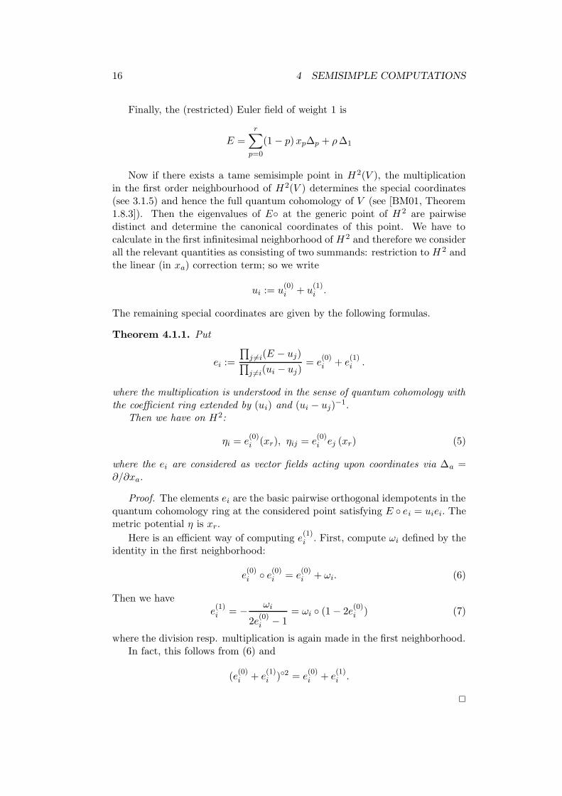
Theorem 4.1.1. Put
ei :=
∏j 6=i(E − uj)∏j 6=i(ui − uj)
= e(0)i + e
(1)i .
where the multiplication is understood in the sense of quantum cohomology withthe coefficient ring extended by (ui) and (ui − uj)−1.
Then we have on H2:
ηi = e(0)i (xr), ηij = e
(0)i ej (xr) (5)
where the ei are considered as vector fields acting upon coordinates via ∆a =∂/∂xa.
Proof. The elements ei are the basic pairwise orthogonal idempotents in thequantum cohomology ring at the considered point satisfying E ei = uiei. Themetric potential η is xr.
Here is an efficient way of computing e(1)i . First, compute ωi defined by the
identity in the first neighborhood:
e(0)i e
(0)i = e
(0)i + ωi. (6)
Then we havee
(1)i = − ωi
2e(0)i − 1
= ωi (1− 2e(0)i ) (7)
where the division resp. multiplication is again made in the first neighborhood.In fact, this follows from (6) and
(e(0)i + e
(1)i )2 = e
(0)i + e
(1)i .
2

4.2 Fano threefolds with minimal cohomology 17
4.2 Fano threefolds with minimal cohomology
4.2.1 Notation
Let V be a Fano threefold. We keep the general notation of the last section,but now consider only the case r = 3. Besides the index ρ, we consider thedegree δ := (c1(V )3)/ρ3 of V.
There exist four families of Fano threefolds V = Vδ with cohomologyHp,p(V,Z) ∼= Z for p = 0, . . . , 3 and Hp,q(V,Z) = 0 for p 6= q. Besides V1 = P3
and the quadric V2 = Q, they are V5 and V22, with degree as subscript; theirindices are, respectively, 4, 3, 2, 1. One can get a V5 by considering a genericcodimension three linear section of the Grassmannian of lines in P4 embeddedin P9.
The nonvanishing β = 0 correlators are coefficients of the cubic self-intersection form
(x0∆0 + · · ·+ x3∆3)3 = δx31 + 3x2
0x3 + x0x1x2 .
In this section, we will deal only with Q, V5 and V22, since projective spacesof any dimension were treated by various methods earlier: see [Man99, II.4]for special coordinates, [Dub98, 4.2.1] and [Guz99] for monodromy data, and[Bar01] for semiinfinite Hodge structures.
4.2.2 Tables of correlators
The following tables provide the coefficients of the multiplication table (4).It suffices to tabulate the primitive correlators, where primitivity means
that ai > 1 and ai ≤ ai+1. The symmetry and the divisor identities furnish theremaining correlators.
Manifold Q:[1; 2,3] [1; 2,2,2] [2; 3,3,3] [2; 2,2,3,3]
1 1 1 1Manifold V5:[1; 3] [1; 2,2] [2; 3,3] [2; 2,2,3] [3; 3,3,3] [2; 2,2,2,2] [3; 2,2,3,3] [4; 3,3,3,3]
3 1 1 1 1 1 2 3Manifold V22:[1; 2] [2; 3] [2; 2,2] [3; 2,3] [4; 3,3] [3; 2,2,2] [4; 2,2,3] [5; 2,3,3]
2 6 1 3 10 1 4 16
[6; 3,3,3] [4; 2,2,2,2] [5; 2,2,2,3] [6; 2,2,3,3] [7; 2,3,3,3] [8; 3,3,3,3]65 2 9 41 186 840
The tables were compiled in the following way. First, (3) furnishes thelist of all primitive correlators that might be (and actually are) non-vanishing.Second, several correlators corresponding to the smallest values of n in (3) mustbe computed geometrically: n = 2 for Q, and n = 1, 2 for V5, and V22. Thesevalues were computed by A. Bondal, D. Kuznetsov and D. Orlov. Third, theassociativity equations uniquely determine all the remaining correlators, in thespirit of the First Reconstruction Theorem of [KM94].
18 4 SEMISIMPLE COMPUTATIONS
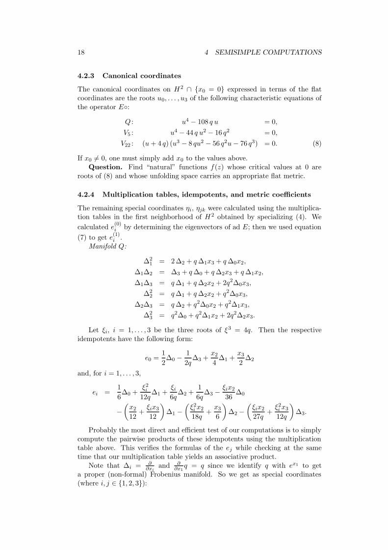
4.2.3 Canonical coordinates
The canonical coordinates on H2 ∩ x0 = 0 expressed in terms of the flatcoordinates are the roots u0, . . . , u3 of the following characteristic equations ofthe operator E:
Q : u4 − 108 q u = 0,
V5 : u4 − 44 q u2 − 16 q2 = 0,
V22 : (u+ 4 q) (u3 − 8 qu2 − 56 q2u− 76 q3) = 0. (8)
If x0 6= 0, one must simply add x0 to the values above.Question. Find “natural” functions f(z) whose critical values at 0 are
roots of (8) and whose unfolding space carries an appropriate flat metric.
4.2.4 Multiplication tables, idempotents, and metric coefficients
The remaining special coordinates ηi, ηjk were calculated using the multiplica-tion tables in the first neighborhood of H2 obtained by specializing (4). We
calculated e(0)i by determining the eigenvectors of ad E; then we used equation
(7) to get e(1)i .
Manifold Q:
∆21 = 2 ∆2 + q∆1x3 + q∆0x2,
∆1∆2 = ∆3 + q∆0 + q∆2x3 + q∆1x2,
∆1∆3 = q∆1 + q∆2x2 + 2q2∆0x3,
∆22 = q∆1 + q∆2x2 + q2∆0x3,
∆2∆3 = q∆2 + q2∆0x2 + q2∆1x3,
∆23 = q2∆0 + q2∆1x2 + 2q2∆2x3.
Let ξi, i = 1, . . . , 3 be the three roots of ξ3 = 4q. Then the respectiveidempotents have the following form:
e0 =1
2∆0 −
1
2q∆3 +
x2
4∆1 +
x3
2∆2
and, for i = 1, . . . , 3,
ei =1
6∆0 +
ξ2i
12q∆1 +
ξi6q
∆2 +1
6q∆3 −
ξix2
36∆0
−(x2
12+ξix3
12
)∆1 −
(ξ2i x2
18q+x3
6
)∆2 −
(ξix2
27q+ξ2i x3
12q
)∆3.
Probably the most direct and efficient test of our computations is to simplycompute the pairwise products of these idempotents using the multiplicationtable above. This verifies the formulas of the ej while checking at the sametime that our multiplication table yields an associative product.
Note that ∆i = ∂∂xi
and ∂∂x1
q = q since we identify q with ex1 to geta proper (non-formal) Frobenius manifold. So we get as special coordinates(where i, j ∈ 1, 2, 3):
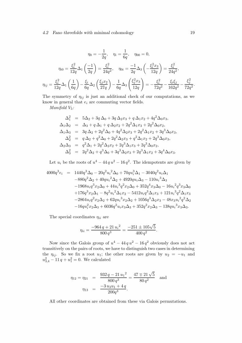
4.2 Fano threefolds with minimal cohomology 19
η0 = − 1
2q, ηi =
1
6q, η00 = 0,
ηi0 =ξ2i
12q∆1
(−1
2q
)=
ξ2i
24q2, η0i =
−1
2q∆3
(−ξ
2i x3
12q
)=
ξ2i
24q2,
ηij =ξ2i
12q∆1
(1
6q
)− ξi
6q∆2
(ξjx2
27q
)− 1
6q∆3
(ξ2jx3
12q
)= − ξ2
i
72q2− ξiξj
162q2−
ξ2j
72q2.
The symmetry of ηij is just an additional check of our computations, as weknow in general that ei are commuting vector fields.
Manifold V5:
∆21 = 5∆2 + 3q∆0 + 3q∆2x3 + q∆1x2 + 4q2∆0x3,
∆1∆2 = ∆3 + q∆1 + q∆2x2 + 2q2∆1x3 + 2q2∆0x2,
∆1∆3 = 3q∆2 + 2q2∆0 + 4q2∆2x3 + 2q2∆1x2 + 3q3∆0x3,
∆22 = q∆2 + q2∆0 + 2q2∆2x3 + q2∆1x2 + 2q3∆0x3,
∆2∆3 = q2∆1 + 2q2∆2x2 + 2q3∆1x3 + 2q3∆0x2,
∆23 = 2q2∆2 + q3∆0 + 3q3∆2x3 + 2q3∆1x2 + 3q4∆0x3.
Let ui be the roots of u4 − 44 q u2 − 16 q2. The idempotents are given by
4000q3ei = 1440q3∆0 − 20q2ui2∆0 + 70qu3
i∆1 − 3040q2ui∆1
−880q2∆2 + 40qui2∆2 + 4920qui∆3 − 110ui
3∆3
−1968uiq3x2∆0 + 44ui
3q2x2∆0 + 352q4x3∆0 − 16ui2q3x3∆0
+176q3x2∆1 − 8q2ui2∆1x2 − 5412uiq
3∆1x3 + 121ui3q2∆1x3
−2864uiq2x2∆2 + 62qui
3x2∆2 + 1056q3∆2x3 − 48x3ui2q2∆2
−16qu2i x2∆3 + 6036q2uix3∆3 + 352q2x2∆3 − 138qui
3x3∆3.
The special coordinates ηii are
ηii =−964 q + 21ui
2
800 q3=−251± 105
√5
400 q2.
Now since the Galois group of u4 − 44 q u2 − 16 q2 obviously does not acttransitively on the pairs of roots, we have to distinguish two cases in determiningthe ηij. So we fix a root u1; the other roots are given by u2 = −u1 andu2
3,4 − 11 q + u21 = 0. We calculated
η12 = η21 =932 q − 21u1
2
800 q3=
47∓ 21√
5
80 q2and
η13 =−3u3u1 + 4 q
200q3.
All other coordinates are obtained from these via Galois permutations.
20 4 SEMISIMPLE COMPUTATIONS
Manifold V22:
∆21 = 22∆2 + 2q∆1 + 24q2∆0
+2q∆2x2 + 48q2∆2x3 + 4q2∆1x2
+27q3∆1x3 + 27q3∆0x2 + 160q4∆0x3,
∆1∆2 = ∆3 + 2q∆2 + 2q2∆1 + 9q3∆0
+4q2∆2x2 + 27q3∆2x3 + 3q3∆1x2
+16q4∆1x3 + 16q4∆0x2 + 80q5∆0x3,
∆1∆3 = 24q2∆2 + 9q3∆1 + 40q4∆0
+27q3∆2x2 + 160q4∆2x3 + 16q4∆1x2
+80q5∆1x3 + 80q5∆0x2 + 390q6∆0x3,
∆22 = 2q2∆2 + q3∆1 + 4q4∆0
+3q3∆2x2 + 16q4∆2x3 + 2q4∆1x2
+9q5∆1x3 + 9q5∆0x2 + 41q6∆0x3,
∆2∆3 = 9q3∆2 + 4q4∆1 + 16q5∆0
+16q4∆2x2 + 80q5∆2x3 + 9q5∆1x2
+41q6∆1x3 + 41q6∆0x2 + 186q7∆0x3,
∆23 = 40q4∆2 + 16q5∆1 + 65q6∆0
+80q5∆2x2 + 390q6∆2x3 + 41q6∆1x2
+186q7∆1x3 + 186q7∆0x2 + 840q8∆0x3.
Now let ui, i = 1, . . . , 3 be the roots of u3 − 8qu2 − 56q2u− 76q3. Then therespective idempotents are given by
5324 q4 ei =(−71742q4 − 24552q3ui + 2354q2ui
2)
∆0
+(−30272q3 − 10186q2ui + 979qui
2)
∆1
+(−118712q2 − 38126qui + 3696ui
2)
∆2
+
(49346q + 16192ui − 1562
ui2
q
)∆3
+(−130876q5 − 43283uiq
4 + 4168ui2q3)x2∆0
+(−483464q6 − 161648uiq
5 + 15528ui2q4)x3∆0
+(−38977q4 − 12940uiq
3 + 1245ui2q2)x2∆1
+(−145898q5 − 48889uiq
4 + 4694ui2q3)x3∆1
+(−143992q3 − 46818uiq
2 + 4522ui2q)x2∆2
+(−491334q4 − 164832uiq
3 + 15822ui2q2)x3∆2
+(35042q2 + 11348uiq − 1098ui
2)x2∆3
+(112272q3 + 37824uiq
2 − 3633ui2q)x3∆3.
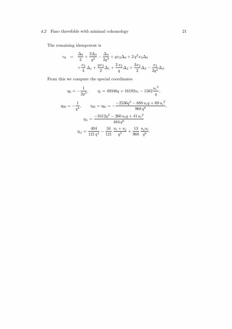
4.2 Fano threefolds with minimal cohomology 21
The remaining idempotent is
e0 =∆0
2+
2∆2
q2− ∆3
2q3+ qx2∆0 + 2 q2x3∆0
+x2
4∆1 +
qx3
2∆1 +
2x2
q∆2 +
3x3
2∆2 −
x2
2q2∆3.
From this we compute the special coordinates
η0 = − 1
2q3, ηi = 49346q + 16192ui − 1562
ui2
q,
η00 = − 1
q4, ηi0 = η0i = −−2536q2 − 688uiq + 69ui
2
968 q6,
ηii =−3412q2 − 260uiq + 41ui
2
484 q6
ηij =404
121 q4− 34
121
ui + ujq5
+13
968
ujuiq6
.

22 4 SEMISIMPLE COMPUTATIONS
23
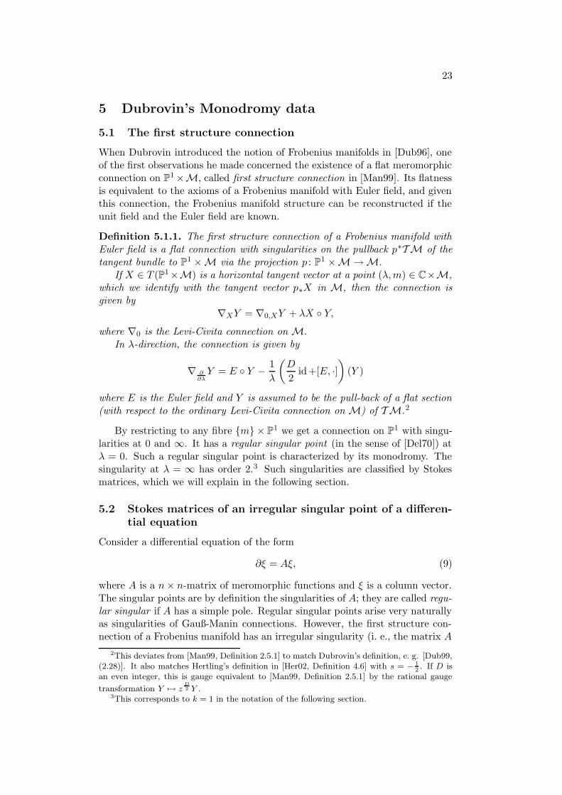
5 Dubrovin’s Monodromy data
5.1 The first structure connection
When Dubrovin introduced the notion of Frobenius manifolds in [Dub96], oneof the first observations he made concerned the existence of a flat meromorphicconnection on P1×M, called first structure connection in [Man99]. Its flatnessis equivalent to the axioms of a Frobenius manifold with Euler field, and giventhis connection, the Frobenius manifold structure can be reconstructed if theunit field and the Euler field are known.
Definition 5.1.1. The first structure connection of a Frobenius manifold withEuler field is a flat connection with singularities on the pullback p∗TM of thetangent bundle to P1 ×M via the projection p : P1 ×M→M.
If X ∈ T (P1×M) is a horizontal tangent vector at a point (λ,m) ∈ C×M,which we identify with the tangent vector p∗X in M, then the connection isgiven by
∇XY = ∇0,XY + λX Y,where ∇0 is the Levi-Civita connection on M.
In λ-direction, the connection is given by
∇ ∂∂λY = E Y − 1
λ
(D
2id +[E, ·]
)(Y )
where E is the Euler field and Y is assumed to be the pull-back of a flat section(with respect to the ordinary Levi-Civita connection on M) of TM.2
By restricting to any fibre m × P1 we get a connection on P1 with singu-larities at 0 and ∞. It has a regular singular point (in the sense of [Del70]) atλ = 0. Such a regular singular point is characterized by its monodromy. Thesingularity at λ = ∞ has order 2.3 Such singularities are classified by Stokesmatrices, which we will explain in the following section.
5.2 Stokes matrices of an irregular singular point of a differen-tial equation
Consider a differential equation of the form
∂ξ = Aξ, (9)
where A is a n× n-matrix of meromorphic functions and ξ is a column vector.The singular points are by definition the singularities of A; they are called regu-lar singular if A has a simple pole. Regular singular points arise very naturallyas singularities of Gauß-Manin connections. However, the first structure con-nection of a Frobenius manifold has an irregular singularity (i. e., the matrix A
2This deviates from [Man99, Definition 2.5.1] to match Dubrovin’s definition, e. g. [Dub99,(2.28)]. It also matches Hertling’s definition in [Her02, Definition 4.6] with s = − 1
2. If D is
an even integer, this is gauge equivalent to [Man99, Definition 2.5.1] by the rational gauge
transformation Y 7→ zD2 Y .
3This corresponds to k = 1 in the notation of the following section.
24 5 DUBROVIN’S MONODROMY DATA
has a second-order pole); the gauge equivalence class of this singularity will bepart of Dubrovin’s classification data of semisimple Frobenius manifolds. Suchan irregular singularity can also arise geometrically in a twisted version of theGauß-Manin connection; this is used to construct Frobenius manifolds fromhypersurface singularities.
Let C(z) be the field of germs of meromorphic function on the complexplane at z = 0, and let C((z)) be the field of formal Laurent series. Differentdifferential equations over C(z) having an irregular singular point can becomegauge equivalent after base change to C((z)). So the classification of irregularsingular differential equations over C(z) can be split in two parts, which are
• classifying differential equations over C((z)), and
• classifying differential equations over C(z) that become isomorphic toa given differential equation over C((z)) after base change.
The datum of Stokes matrices is one possible classification datum for thesecond step.
Differential modules and differential equations. As we will freely changeour point of view between differential modules and that of differential equations(or rather their gauge equivalence classes), we feel obliged to spell out preciselyhow to pass from one to another.4
Definition 5.2.1. A differential ring is a ring R (commutative, with iden-tity) equipped with a derivation ∂ : R → R satisfying the Leibniz rule ∂(rr ′) =∂(r)r′ + r∂(r′).
We will consider the differential rings C((z)), C(z) with ∂∂z as the structure
derivation.
Definition 5.2.2. A differential module over a differential ring R is a locallyfree R-module M equipped with a derivation ∂M : M →M satisfying the Leibnizrule ∂M (r.m) = ∂(r).m+ r.∂M (m).
Definition 5.2.3. A matrix differential equation over R is an equation of theform
∂ξ = Aξ
where A is a n × n-matrix over R. Two such equations given by matrices Aand A′ are called gauge equivalent if one can be obtained from the other by agauge transformation ξ = Fξ ′: This is the case iff A′ = F−1(AF + ∂F ) with Fan invertible n× n-matrix over R.
Of course, we always think of the indeterminate ξ as a column vector withentries in (some extension of) R.
4Some proofs will require coordinates, and hence the point of view of differential equations,yet at least in my case the word “differential module” is more likely to trigger some conceptualthinking—my apologies go to those readers whose mathematical thinking would not need thisspecific abstract nonsense.
5.2 Stokes matrices of an irregular singular point of a differential equation 25
We can pass from 5.2.3 to 5.2.2 by defining M to be Rn and its derivationas ∂Mξ := ∂ξ − Aξ. If the ground ring is a field (or the differential module isfree as an R-module), we can go the other way by choosing a basis ξ1, . . . , ξnof M ; then A is the matrix expressing ∂Mξ1, . . . , ∂M ξn in terms of this basis.Another choice of a basis yields a gauge equivalent differential equation.
In this dictionary, fundamental matrix solutions of the differential equationcorrespond to trivializations of the differential module.
If, instead of a differential ring, we are given a topological space equippedwith a sheaf of differential rings O, it is immediately clear what we mean by asheaf of differential modules over the sheaf O. We will call this a differentialO-module.
We can get differential modules from a connection on an O-module M: Ifwe choose any vector field X, we get derivations on O and M by ∂ : f 7→ Xfand ∂M : s 7→ ∇Xs. In our case of the first structure connection on P1, this willbe a coordinate vector field ∂
∂z .Note that we also have to choose one such vector field X. In that sense, the
whole theory is one-dimensional.
Differential modules over C((z)). From now on, δ will denote the differ-ential operator
δ = z∂
∂z.
Over the field C((z)) of formal Laurent series, the following theorem com-pletely classifies differential modules:
Theorem 5.2.4. [vdPS03] Let M be a finite dimensional differential module
over C((z)). Then there is a finite algebraic extension C((z1k )), such that after
base change M becomes a split differential module: M is isomorphic to thedirect sum of differential modules Mi given by an equation of the form
δξ = (qi + Ci)ξ
where qi is a polynomial in z−1kC[z−
1k ] and C ∈ Matn×n(C) is a n× n-matrix
(and δ is defined as above). The qi are unique, and the matrices Ci are uniqueup to shifts by integers.
The fundamental short exact sequence. The whole theory of Stokes ma-trices is based upon a short exact sequence of sheaves on S1. Here S1 is identifiedwith the set of rays in the complex plane starting in the origin, and hence anopen set U ⊂ S1 is seen as an open sector.
In the following, we will omit the proofs of all analytical lemmata andonly focus on the algebraic structure of the theory. The exposition is close to[vdPS03], where all proofs can be found.
Definition 5.2.5. The sheaf A of functions with asymptotic expansion is de-fined as follows: If U ⊂ S1 is a connected open subset, then A(U) consists ofgerms at zero of functions f on the open sector U such that there exists anasymptotic expansion
∑n≥n0
cnzn of f ; this means that for every closed subset
26 5 DUBROVIN’S MONODROMY DATA
W ⊂ U there exist constants C(N,W ) such that on an open neighbourhood ofzero in W we have
|f(z)−N−1∑
n=n0
cnzn| < C(N,W )zN .
Note that the asymptotic expansion, if it exists, is uniquely defined by f ,so there is a canonical map α from A to the constant sheaf C((z)). However,
the asymptotic expansion does not define f uniquely, and the map A α→C((z))
has a kernel A0 which consists of germs of rapidly vanishing functions. Typicalsections of A0 are of the form eaz
−kin a sector where az−k has negative real
part.
Note that
A(S1) = C(z) and A0(S1) = 0;
also, the following holds:
Lemma 5.2.6. [vdPS03, proposition 7.22] The map of sheaves α : A→ C((z))
is surjective; more precisely, α(U) : A(U)→ C((z))(U) is surjective iff U 6= S 1.
Thus there is a short exact sequence
0→ A0 → A α→C((z))→ 0
of sheaves on S1.
The additive Stokes phenomenon: The one-dimensional case. Letq = akz
−k + · · · + a1z−1 be an arbitrary polynomial. Consider the differential
equation
(δ − q)v = w
where w ∈ C(z) is a given germ of a meromorphic function and v ∈ C((z))is a given formal solution. We want to know whether this formal solution canbe lifted over an open sector U ⊂ S1 to a solution v ∈ A(U) which has v as anasymptotic expansion.
To reduce this to a purely algebraic problem we need one more lemma:
Lemma 5.2.7. [vdPS03] There is a short exact sequence
0→ ker(δ − q|A0)→ ker(δ − q|A)→ ker(δ − q|C((z)))→ 0
of sheaves on S1. Furthermore, the map δ − q locally acts surjectively on eachof the sheaves A, A0 and C((z)).
Proof. We omit the proof of the second part of the assertion. The first partfollows from the second by the 9-lemma (applied to the diagram given in theproof of the next lemma).
From this, the following is easily deduced:
5.2 Stokes matrices of an irregular singular point of a differential equation 27
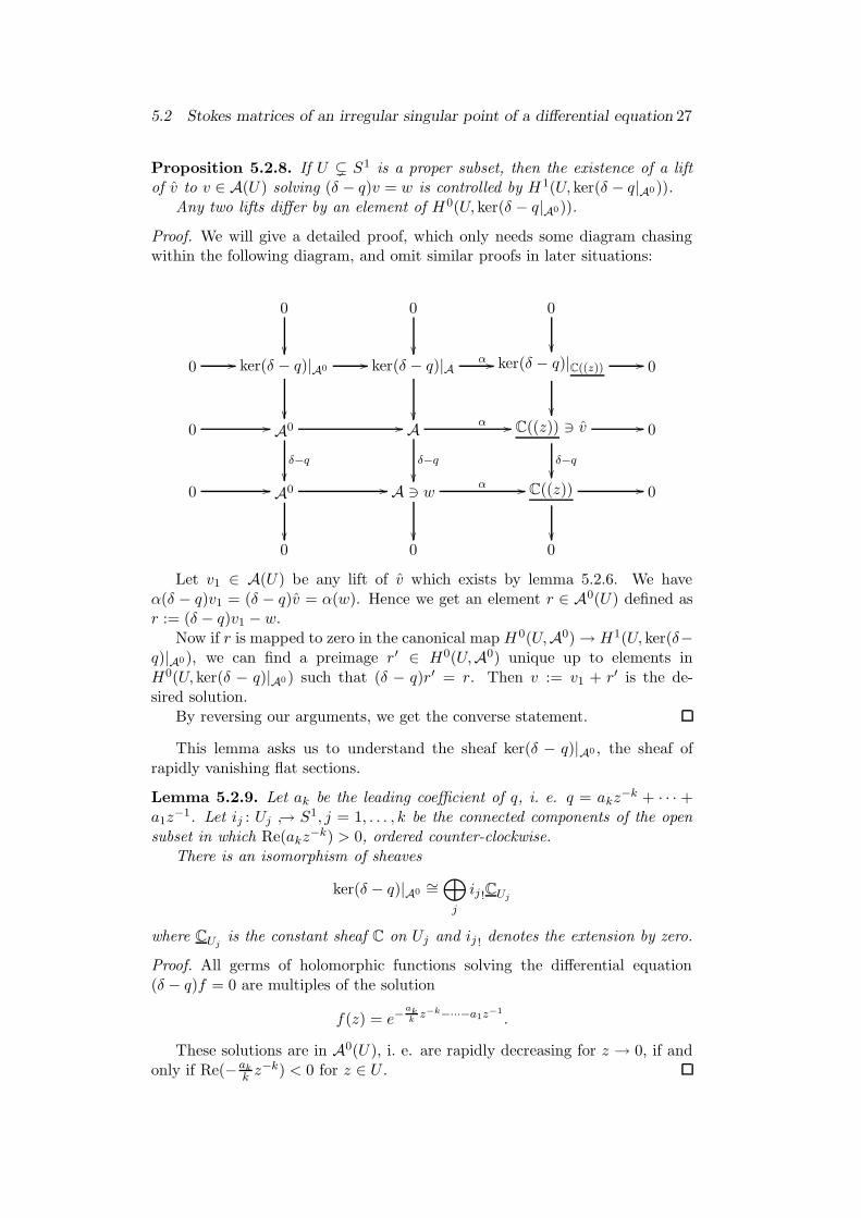
Proposition 5.2.8. If U ( S1 is a proper subset, then the existence of a liftof v to v ∈ A(U) solving (δ − q)v = w is controlled by H 1(U, ker(δ − q|A0)).
Any two lifts differ by an element of H0(U, ker(δ − q|A0)).
Proof. We will give a detailed proof, which only needs some diagram chasingwithin the following diagram, and omit similar proofs in later situations:
0
0
0
0 // ker(δ − q)|A0
// ker(δ − q)|A
α // ker(δ − q)|C((z))
// 0
0 // A0
δ−q
// Aδ−q
α // C((z)) 3 v
δ−q
// 0
0 // A0
// A 3 w
α // C((z))
// 0
0 0 0
Let v1 ∈ A(U) be any lift of v which exists by lemma 5.2.6. We haveα(δ − q)v1 = (δ − q)v = α(w). Hence we get an element r ∈ A0(U) defined asr := (δ − q)v1 − w.
Now if r is mapped to zero in the canonical map H0(U,A0)→ H1(U, ker(δ−q)|A0), we can find a preimage r′ ∈ H0(U,A0) unique up to elements inH0(U, ker(δ − q)|A0) such that (δ − q)r′ = r. Then v := v1 + r′ is the de-sired solution.
By reversing our arguments, we get the converse statement.
This lemma asks us to understand the sheaf ker(δ − q)|A0 , the sheaf ofrapidly vanishing flat sections.
Lemma 5.2.9. Let ak be the leading coefficient of q, i. e. q = akz−k + · · · +
a1z−1. Let ij : Uj → S1, j = 1, . . . , k be the connected components of the open
subset in which Re(akz−k) > 0, ordered counter-clockwise.
There is an isomorphism of sheaves
ker(δ − q)|A0∼=⊕
j
ij !CUj
where CUj is the constant sheaf C on Uj and ij ! denotes the extension by zero.
Proof. All germs of holomorphic functions solving the differential equation(δ − q)f = 0 are multiples of the solution
f(z) = e−akkz−k−···−a1z−1
.
These solutions are in A0(U), i. e. are rapidly decreasing for z → 0, if andonly if Re(−ak
k z−k) < 0 for z ∈ U .
28 5 DUBROVIN’S MONODROMY DATA
The border lines of the sectors Uj are called the Stokes rays of the differentialequation.
From the cohomology of the sheaf CS1 and of the cokernel of ker(δ−q)|A0 →CS1 (which is the direct sum
⊕j ij∗CVj where Vj is the closed sector in between
Uj and Uj+1), we can immediately compute the cohomology of ker(δ − q)|A0):
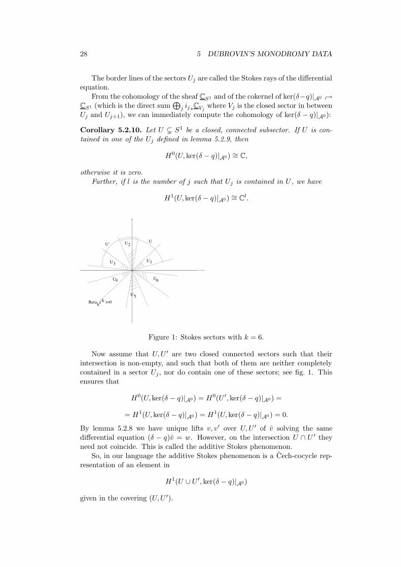
Corollary 5.2.10. Let U ( S1 be a closed, connected subsector. If U is con-tained in one of the Uj defined in lemma 5.2.9, then
H0(U, ker(δ − q)|A0) ∼= C,
otherwise it is zero.Further, if l is the number of j such that Uj is contained in U , we have
H1(U, ker(δ − q)|A0) ∼= Cl.
U
U1
U2
U3
4
U5
U6
kRe(a z )=0-k
UU’
Figure 1: Stokes sectors with k = 6.
Now assume that U,U ′ are two closed connected sectors such that theirintersection is non-empty, and such that both of them are neither completelycontained in a sector Uj , nor do contain one of these sectors; see fig. 1. Thisensures that
H0(U, ker(δ − q)|A0) = H0(U ′, ker(δ − q)|A0) =
= H1(U, ker(δ − q)|A0) = H1(U, ker(δ − q)|A0) = 0.
By lemma 5.2.8 we have unique lifts v, v ′ over U,U ′ of v solving the samedifferential equation (δ − q)v = w. However, on the intersection U ∩ U ′ theyneed not coincide. This is called the additive Stokes phenomenon.
So, in our language the additive Stokes phenomenon is a Cech-cocycle rep-resentation of an element in
H1(U ∪ U ′, ker(δ − q)|A0)
given in the covering (U,U ′).
5.2 Stokes matrices of an irregular singular point of a differential equation 29
Higher dimensional additive Stokes phenomena. The preceding sectionis easily generalized to the case of a higher-dimensional differential equation:We consider the differential equation
(δ −A)v = w (10)
where A is a n×n-matrix with coefficients in C(z), w ∈ C(z)n is fixed andv ∈ C((z))n is a given solution; again we are considering the problem whetherthere exists a lift of v to an element v ∈ A(U)n that has v as asymptoticalexpansion.
As in the one-dimensional case, we omit the proof of the
Lemma 5.2.11. [vdPS03, Theorem 7.12] Let A be any n×n-matrix with entriesin C(z).
The operator δ−A yields surjective endomorphisms of the sheaves An, (A0)n
and C((z))n. There is a short exact sequence
0→ ker(δ −A)|(A0)n → ker(δ −A)|An → ker(δ −A)|C((z))n → 0
of sheaves on S1.
With the same proof as in the last section, we get from this:
Proposition 5.2.12. Consider the differential equation (10), and let U ( S 1
be a proper open subset. Then existence and non-uniqueness of a lift v ∈ A(U)n
of v that solves the same differential equation are controlled by the cohomologyH0 and H1 on U of the sheaf ker(δ −A)|(A0)n .
At the moment, we can not yet compute the cohomology of this sheaf; weonly note that such a lift exists locally, i. e. if U is sufficiently small.
Of course, we can rephrase the statements of this section in the language ofdifferential modules: If M is a differential module over C(z), we can associate
to it in an obvious manner the sheaves of differential modules M0, M and Mon S1 over the sheaves of rings A0, A and C((z)), respectively. If M0f ,Mf
and Mf , denote the respective subsheaves of flat sections (which we wrote asM0f = ker(δ − A)|(A0)n etc.), then the short exact sequence of lemma 5.2.11reads as
0→M0f →Mf → Mf → 0.
Everything else translates in a similar way.
The key idea. Given a differential module N over C(z), we want to un-derstand which differential modules become isomorphic to N after base changeto C((z)).
In coordinates, if M and N are given by differential equations δ − A andδ − B, a formal isomorphism of M and N means the following: There exists amatrix F ∈ GL(n,C((z))) that satisfies the differential equation
δF = AF − FB. (11)
30 5 DUBROVIN’S MONODROMY DATA
(This differential equation is equivalent to the statement that F gives a gaugeequivalence between the two differential equations (δ−B)ξ = 0 and (δ−A)F ξ =0.)
Now the essential idea of the theory of Stokes matrices is to apply the theorydeveloped in the previous two sections to the differential equation (11). So wetreat the n× n-matrix F as a column vector with n2 entries, and we note that(11) is of the same form as (10). We immediately get from the remark afterproposition 5.2.12 that, locally in S1, we can find a matrix solution F of (11)with entries in A(U) that has F as asymptotic expansion.
We can rephrase this more abstractly. Let M and N be the sheaves of dif-ferential modules over the sheaf of rings A associated to M and N , respectively.
Lemma 5.2.13. Locally in S1, the differential A-modules M and N are iso-morphic (as differential A-modules).
This fact encourages directly the following definition and proposition:
Definition 5.2.14. Given the differential A-module N , let AutN be the sheafof A-module automorphisms of N . It has a subsheaf (AutN )f of flat sectionswhich consists of the automorphisms of N as a differential A-module.
The sheaf Aut0N will denote the subsheaf of endomorphisms that have theidentity as asymptotic expansion (that is, expressed in an arbitrary A-basis,the endomorphism is represented by a matrix that has the identity matrix asasymptotic expansion). Of course (Aut0N )f denotes the corresponding subsheafof flat sections.
Since the differential module M is obviously determined by its associatedsheaf M, one gets nearly automatically the
Proposition 5.2.15. Let N be a differential module over C(z). Every dif-ferential module M over C(z) that is formally isomorphic to N is determinedby an element in H1(S1, (Aut0N )f ).
Proof. We fix an isomorphism F : M∼→ N . We cover S1 by open subsets Ui
such that on each Ui, we have M|Ui ∼= N|Ui by a chosen isomorphism γi;we require that γi has F as asymptotic expansion. On the overlaps Ui ∩ Uj ,we get elements γij = γi γ−1
j as usual. By our choices, the automorphisms
γij have Id as asymptotic expansion: γij ∈ (Aut0N )f (Ui ∩ Uj). So the γijyield a Cech-cocycle in H1(S1, (Aut0N )f ), from which the sheaf M can bereconstructed.
The Malgrange-Sibuya Theorem. The proof of the following theorem ismore involved than the proofs so far (and omitted here); the result is a majorstep in the classification of irregular differential modules:
Theorem 5.2.16. The natural map H1(S1,Aut0N ) → H1(S1,AutN ) hasimage 1.
(Remember that sections of AutN are just the A-module endomorphismsof the A-module N ; so in fact we have AutN ∼= GL(n,A).)
5.2 Stokes matrices of an irregular singular point of a differential equation 31
Corollary 5.2.17. Given a differential module N over C(z), there is a 1 : 1-correspondence between
• differential modules M over C(z) equipped with an isomorphismM ⊗C(z) C((z)) ∼= N ⊗C(z) C((z)), and
• elements of H1(S1, (Aut0N )f ).
Proof. By proposition 5.2.15, it only remains to show that to every elementγ ∈ H1(S1, (Aut0N )f ), we can find a differential module M which is sent to γin the map described in this proposition.
By the short exact sequence
1→ Aut0N → AutN → AutN → 1
and the Malgrange-Sibuya Theorem we can find a global section F ∈H0(S1, AutN ) ∼= GL
(n,C((z))
)which is mapped to the same element in
H1(S1,Aut0N ) as γ; the choice of F is unique up to elements inH0(S1,AutN ),which will not affect the differential module we are going to construct.
If N corresponds to the matrix differential equation δ − B, we would liketo define M via the differential equation δ − A = F−1(δ − B)F ; however, itis unclear whether the matrix A defined by this equation will have convergententries. So we will again use our fundamental short exact sequence to constructA:
We can cover S1 by open sets Ui such that on each open set, F can be liftedto an element Fi ∈ (AutN )(Ui) having F as asymptotic expansion; we canchoose the Fi in such a way that (FiF
−1j )ij is a Cech-cocycle representing γ in
H1(S1, (Aut0N )f ). We define Ai ∈ GL(n,A(Ui)) on Ui by the equation
δ −Ai = F−1i (δ −B)Fi.
By our choice, the FiF−1j define differential automorphisms of N on Ui∩Uj,
hence they commute with δ −B. Thus we get
F−1i (δ −B)Fi = F−1
j (δ −B)Fj,
which implies Ai|Ui∩Uj = Aj |Ui∩Uj . So the Ai glue to a well-defined globalsection A ∈ H0(S1,GL(n,A)) = GL(n,C(z)) which defines the differentialmodule M as desired.
Stokes matrices with respect to adjacent sectors. We make the follow-ing simplifying assumption:
Assumption 5.2.18. We assume that after base change to C((z)), the differ-ential module M splits: We have
M ⊗C C((z)) ∼=⊕
i
Qi ⊗C C((z))
where each Qi is isomorphic to the one-dimensional differential module associ-ated to the scalar differential equation (δ − qi), and each qi ∈ z−1C[z−1] is apolynomial in z−1 of the same degree k for all i. Further, we assume that forall pairs i 6= j, the polynomial qi − qj is of degree k as well.
32 5 DUBROVIN’S MONODROMY DATA
This assumption contains three simplifications (compare with Theo-rem 5.2.4):
• In general, such a decomposition exists only after adjoining some root k√z
to C((z)),
• the decomposition could contain higher dimensional irreducible modulesassociated to a differential equation of the form δ − qi + Ci with someconstant n× n-matrix Ci, and
• the qi and their differences qi − qj could have different degrees.
While the first two simplifications rather just shorten our notation, the thirddoes make a substantial difference. Without it, one needs a filtration on thesheaves A0,A,C((z)) such that (very roughly speaking) each filtration steponly notices the effects of those summands Qi where qi is a polynomial of fixeddegree; the main ingredient is then the so-called multisummation theorem.
Let N be the differential module N =⊕
iQi over C(z). We are given an
element γ of Hom(M,N); it corresponds to the matrix F of equation (11). Asin the additive Stokes phenomenon, we are looking for sectors U on which γcan be lifted uniquely to an element γ(U) ∈ Hom(M,N ). Since we obviously
have Hom(M,N) ∼= End(N), the following lemma will be useful:
Lemma 5.2.19. Assume that the differential modules L, L are formally isomor-phic. Then the associated sheafs L0f and L0f of rapidly vanishing flat sectionsare isomorphic.
We apply this to L = Hom(M,N) and L = End(N). Using our assumptions,it is easy to describe the sheaf (EndN)0f :
Lemma 5.2.20. Let N =⊕
iQi be as above. Each Qi is the one-dimensionaldifferential module associated to the differential equation δ − qi with
qi = aikz−k + · · ·+ ai1z
−1.
For each pair i 6= j let fij be the standard solution to the differential equation(δ + qi − qj)fij = 0 which is given by
fij = eaik−ajk
kz−k+···.
Now let Uij be the union of the k sectors where fij has zero as asymptoticalexpansion, i. e. where Re(aik − ajk)z−k < 0.
The claim is that
(EndN)0f =⊕
i6=j(iUij )!C.
Proof. Indeed, there are no non-zero rapidly vanishing differential endomor-phisms of Qi, and gauge transformations from the differential equation δ − qito δ − qj are exactly given by (a constant multiple of) such a function fij.
5.2 Stokes matrices of an irregular singular point of a differential equation 33
So if U neither does contain nor is contained in any of the k connectedcomponents of Uij for any pair i, j, we have
H0(U, (Hom0(M,N))f ) = H1(U, (Hom0(M,N))f ) = 0. (12)
This is satisfied for almost all connected sectors U of length πk .
Now suppose we have two such connected sectors U and U ′ with non-emptyconnected overlap U ∩U ′. By proposition 5.2.12 there are unique lifts γU , γU ′ ofγ on these open sets. Their difference γ−1
U ′ γU is an element of (Aut0N )f (U ∩U ′).
After adjoining the solutions fi = e−aikk
z−k+··· of the differential equationsδ − qi, i = 1 . . . n to our base field, the sheaf N has a canonical basis of flatsections. This yields an isomorphism (AutN )f (U ∩ U ′) ∼= GL(n,C) by repre-senting each automorphism with respect to this flat basis.
We need to identify the image of (Aut0N )f (U ∩ U ′) in GL(n,C). Fromlemma 5.2.20 it is clear that it consists of n× n-matrices K that
• have Kii = 1 on the diagonal, and
• whose non-diagonal entries Kij vanish unless U ∩ U ′ ⊂ Uij .Now let us consider γ−1
U ′ γU ∈ (Aut0(N ))f (U ∩ U ′). Under the aboveisomorphism, this yields a matrix S of complex numbers satisfying the twoconditions described above. The matrix S is the Stokes matrix of M withrespect to the sectors U and U ′.
Stokes matrices. Now we know everything to go ahead and actually con-struct the collection of Stokes matrices associated to a differential module Msatisfying the assumption 5.2.18:
1. Choose an isomorphism M ∼=γ⊕n
i=1Qi = N as in 5.2.18. This includesthe choice of an ordering of the irreducible modules.
2. Choose an appropriate covering U1, . . . , Um of S1 by connected open sec-tors Uj . Each Ui must satisfy the condition necessary to ensure (12); thisis automatically true if they are of size marginally larger than π
k and ingeneral position. We will assume that they are ordered counter-clockwiseon S1.
To produce such a covering, we start with an arbitrary U1 satisfying thecondition. Having chosen U1, . . . , Ul−1 or U ′1, . . . , U
′l−1 respectively, we
can either
(a) choose U ′l “as close as possible” to U ′l−1—by this we mean that U ′l ∩U ′l−1 is only contained in Uij (defined in proposition 5.2.20) for asingle pair i, j (or several pairs only if the corresponding sectors Uijand Ui′j′ coincide)—, or we can
(b) choose Ul “as far away as possible” from Ul−1. This means thatUl ∩ U ′l−1 is contained in as many sectors Uij as possible, i. e. in allsuch sectors that contain the relevant border line of Ul−1.

34 5 DUBROVIN’S MONODROMY DATA
The two different coverings obtained by starting with the same open sectorU1 = U ′1 are shown in figure 5.2.
U21U23
U32
U32
U13
U13
U31
U’1
U3
U4
U31
U21U23
U12
U12
U2
1U =
U’
U’
U’
U’2
3
4
5
Figure 2: The two coverings (with k = 2 and n = 3): U1, U2, U3, U4 andU ′1, U ′2, U ′3, U ′4, U ′5, . . .
As explained in the previous section, we get a Stokes matrix Sl associated toeach pair of sectors Ul, Ul+1 (respectively a matrix Kl from U ′l , U
′l+1). It is the
matrix representation of γUl γ−1Ul−1
with respect to the flat basis of N|Ul∩Ul+1.
Using (2a), we get 2k ·(n
2
)of these matrices, compared to only 2k if we choose
method (2b).The procedure using (2a) is more canonical: Every choice of U1 will
produce—up to cyclic reordering—the same Stokes matrices S1, . . . , Sm. Eachsuch matrix will have only one non-zero off-diagonal entry at i, j whereUl ∩ Ul−1 ⊂ Uij (unless some of the sectors Uij are identical).
We will follow Dubrovin’s terminology (see [Dub99]) and call the matricesKl obtained by method (2a) Stokes factors; then only the matrices Sl that weget using method (2b) will be called Stokes matrices. Up to reordering of thebasis, the latter are alternatingly upper and lower triangular matrices. Stokesmatrices and Stokes factors can easily be reconstructed from each other purelyalgebraically. This is due to the constraints on the matrices Kl and the relationsbetween the two sets of matrices:
Si = Ki·(n2)·Ki·(n2)−1 · . . . · · ·K(i−1)·(n2)+1.
5.3 Stokes matrices of a Frobenius manifold
As we explained in the beginning of this chapter, the Stokes matrices of agenerically semisimple Frobenius manifold are the Stokes matrices at λ =∞ ofits first structure connection.
So assume that we have chosen a semisimple pointm ∈M. Let u1, . . . , un bethe canonical coordinates. We assume that they are pairwise distinct; otherwisethe assumption 5.2.18 would not hold.
Now consider the first structure connection of M restricted to m × P1.The idempotents ∂
∂uiform a natural basis of p∗TM|m×M.
5.3 Stokes matrices of a Frobenius manifold 35
Let z = 1λ . At z = 0, the connection yields a differential module M over
C(z). Recalling the definition of the first structure connection, we see thatits differential equation is
δv =1
zE v − [E, v].
(Here [E, v] denotes the Lie bracket of E with the flat extension of v ∈ TmMto a neighbourhood of m.)
Let Qi be the one-dimensional differential module associated to the equation
δv =uizv.
We see immediately that M and⊕n
i=1Qi are isomorphic up to O(1) via theisomorphism of vector spaces γ that sends ∂
∂uito 1 ∈ Qi. In fact, there exists
a unique formal isomorphism
M ⊗ C((z))γ∼=
n⊕
i=1
Qi ⊗ C((z)) (13)
of differential modules that agrees with γ up to higher orders of z: γ = γ+O(z).The proof is easy but not very enlightening (cf. [Dub99, lemma 4.3]): It justconstructs γ step by step as a power series.
So we have found a natural choice for step (1) in the construction of Stokesmatrices as described above; using step (2a) above we only lack a choice of U1.
There is no natural choice here. We can just note that U1 will be a connectedopen sector of size approximately π. Then U2 is a sector of similar size thathas small overlaps with U1 at both ends. Together, they cover S1. From thetwo connected components of U1 ∩U2, we get two Stokes matrices S1, S2 of ourFrobenius manifold.
These two matrices are related via
S2 = ST1 . (14)
This follows from the good behaviour of γ with respect to the metric that Minherits from the metric of the Frobenius manifold.
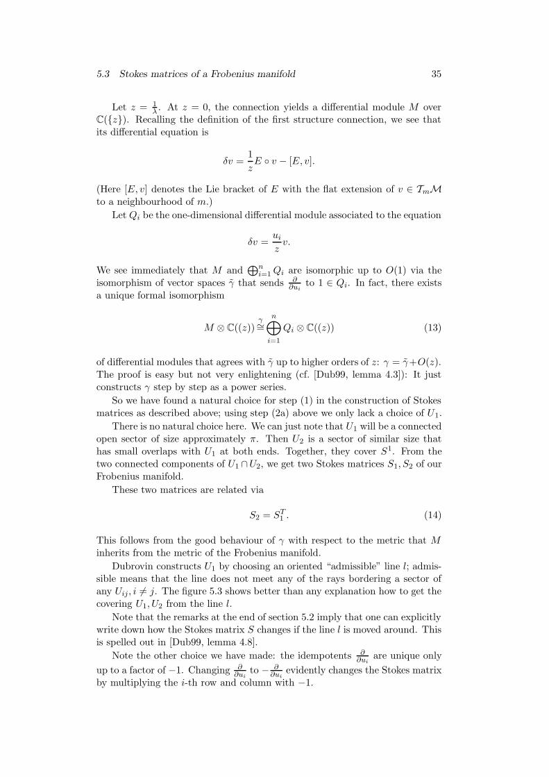
Dubrovin constructs U1 by choosing an oriented “admissible” line l; admis-sible means that the line does not meet any of the rays bordering a sector ofany Uij, i 6= j. The figure 5.3 shows better than any explanation how to get thecovering U1, U2 from the line l.
Note that the remarks at the end of section 5.2 imply that one can explicitlywrite down how the Stokes matrix S changes if the line l is moved around. Thisis spelled out in [Dub99, lemma 4.8].
Note the other choice we have made: the idempotents ∂∂ui
are unique only
up to a factor of −1. Changing ∂∂ui
to − ∂∂ui
evidently changes the Stokes matrixby multiplying the i-th row and column with −1.

36 5 DUBROVIN’S MONODROMY DATA
U23
U32
U13
U31
U12
U21
l
U
U1
2
Figure 3: The admissible line l and the covering U1, U2
5.4 Dubrovin’s monodromy data
Dubrovin’s monodromy data is a list of invariants of the first structure con-nection (more precisely of a fibre m × P1 of the connection) that suffice tocharacterize it.
The Stokes matrix S = S1, together with the canonical coordinates, classifiesthe singularity at λ =∞ of the first structure connection. More precisely, fromthis we can reconstruct the connection ∇U∞ in a neighbourhood U∞ of infinity.
Dubrovin’s list begins with a vector space V that is identified with the spaceof flat sections of the connection (and will become the tangent space TmM) anda symmetric bilinear form g on V that will become the metric of the Frobeniusmanifold.
As mentioned before, the singularity of the connection at λ = 0 is a regularsingularity. A classical invariant of such a point is the residue endomorphismµ ∈ End (V ) of the connection ∇ ∂
∂λ(as defined in [Del70, II.1.16]).
As can be read off from the definitions, we have µ = −D2 id−[E, ·]. This
endomorphism is antisymmetric with respect to the metric g, and we assumethat it is diagonalizable.
Further, Dubrovin defines an endomorphism R by the following properties:
• It can be written as a finite sum R = R1 + R2 + . . . , such that thefirst structure connection is gauge equivalent (by a gauge transformationholomorphic on C) to
∇ ∂∂λv = ∂λv + (
1
λµ+R1 + λR2 + λ2R3 + . . . )v.
• The endomorphisms R2k+1 are symmetric with respect to g, the R2k areantisymmetric.
• Let V =⊕
r Vr be the isotypical decomposition of V with respect to µ,i. e. µ|Vr = r · id. Then Rk(Vr) ⊂ Vr+k.
5.4 Dubrovin’s monodromy data 37
The tuple (V, g, µ,R) fully describes the restriction ∇|C of the connectionto C.
Finally, we have to understand how ∇|C and ∇U∞ glue to the connection∇ on P1. This glueing is determined by the identification of the spaces of flatsections on any simply connected subset of C ∩ U∞.
Around λ =∞, we have a canonical basis of flat sections on the open sectorU1 in the
(z = 1
λ
)-plane: the lift γ1 of the formal isomorphism γ defined in
equation (13) is holomorphic on U1. The space of flat sections of⊕
iQi (as
defined in section 5.3) is identified with Cn via Cn 3 ei 7→ e−uiz · 1 ∈ Qi.
From λ = 0, the space of flat sections around any point is identified with V .Thus the glueing of the two connections is given by an isomorphism C : Cn → V .Dubrovin calls this the central connection matrix.
This completes the list of Dubrovin’s monodromy data. An immediate goodargument in favor of their usefulness is the following theorem:
Theorem 5.4.1. [Dub99] With a consistent choice of the oriented line l ⊂ C,the monodromy data (V, g, µ,R, S,C) does not depend on the choice of the basepoint m ∈M.
It is not clear for which set of data (V, g, µ,R, S,C) a Frobenius manifoldexists. One relation is obtained by comparing the monodromy around ∞ withthat around 0. However, there are further implicit relations that can onlybe phrased by the solvability of a Riemann-Hilbert boundary value problem:Starting with arbitrary values, it is not clear whether the identification of flatsections specified by C extends to glue the sheaves V ⊗ OC and
⊕iQi to a
globally free sheaf on P1.

38 5 DUBROVIN’S MONODROMY DATA
39
6 Exceptional systems and Dubrovin’s conjecture
6.1 Exceptional systems in triangulated categories
We consider a triangulated category C. We assume that it is defined over aground field k, i. e. for each pair of objects A, B, the morphisms HomC(A,B)form a k-vector space. In our examples, C will always be the bounded derivedcategory Db(X) of coherent sheaves on a variety X/k.
In a way, exceptional objects in triangulated categories are a substitute forsimple objects in abelian categories; an exceptional system vaguely correspondsto the list of simple objects in a semisimple abelian category.
Definition 6.1.1. • An exceptional object in C is an object E such that theendomorphism complex of E is concentrated in degree zero and equal to k:
RHom•(E , E) = k[0]
• An exceptional collection is a sequence E0, . . . , Em of exceptional objects,such that for all i > j we have no morphisms from Ei to Ej:
RHom•(Ei, Ej) = 0 if i > j
• An exceptional collection of objects is called a complete exceptional col-lection (or exceptional system), if the objects E0, . . . , Em generate C as atriangulated category: The smallest subcategory of C, that contains all Ei,and is closed under isomorphisms, shifts and cones, is C itself.
The basic example is the bounded derived category Db(Pn) on a projectivespace with the series of sheaves O(i),O(i + 1), . . . ,O(i + n) (for any i). Thiswas first observed (together with the special case of the Theorem 6.1.2) byBeılinson (cf. [Beı84]). Later, exceptional systems were studied by a group atthe Moscow University, see e. g. the collection of papers in [Rud90].
The length of an exceptional system in Db(X) always equals the dimensionof the cohomology of X, in fact an exceptional collection is complete if and onlyif its length is dimkH
∗(X).To justify our vague claim about the correspondence to semisimple abelian
categories we cite the following theorem, which is due to Bondal. It may beconsidered as a derived non-commutative analogue to the classical theorem onthe structure of semisimple abelian categories:
Theorem 6.1.2. [Bon89, Theorem 6.2] Assume that the exceptional systemE0, . . . , Em of the category C satisfies the following additional property: Foreach i < j, the complex RHom•(Ei, Ej) is concentrated in degree zero.
Let A be the algebra of endomorphisms of⊕
i Ei. Then C is equivalent tothe derived category Db(A) of right A-modules.
It seems very plausible that it is possible to drop this additional assumptionif we replace
• the triangulated category C by a differential graded category and
40 6 EXCEPTIONAL SYSTEMS AND DUBROVIN’S CONJECTURE
• the endomorphism algebra A by the DG algebra of endomorphisms of⊕i Ei.
Indeed, this has been proven (but not yet published) by B. Keller. A versionwith A∞-algebras and A∞-categories is possible as well.
Examples of varieties that do have an exceptional system include projectivespaces or, more generally, flag varieties.
6.2 Dubrovin’s conjecture
We are now ready to give the precise formulation of Dubrovin’s conjecture.
Conjecture 6.2.1. [Dub98] Let X be a Fano variety.
Claim 1: The quantum cohomology of X is generically semisimple if andonly if there exists an exceptional system in its derived category Db(X).
Claim 2: In this case, define the Stokes matrix Sij via the Euler characteristicsof the exceptional system:
Sij := χ(Ei, Ej)
This is an upper triangular matrix with ones on the diagonal. On the otherhand, consider the Stokes matrix S1 associated to the Frobenius manifoldof the Quantum cohomology of X.
With an appropriate choice of a semisimple point and of the admissibleline l producing the covering U1, U2 ⊂ S1, the Stokes matrix S1 is givenby S1 = Sij.
Claim 3: Finally, let C ′′ : Cn → H∗(X) be the isomorphism that sends ei tothe Chern character Ch(Ei). The central connection matrix C of theFrobenius manifold can be written as
C = C ′C ′′
where C ′ is an endomorphism of H∗(X) that commutes with multiplica-tion by the first chern class of X. (The precise nature of C ′ in generalis yet unclear.)
41
7 Semisimple mirror symmetries
This section will vaguely explain how Dubrovin’s conjecture fits into the contextof mirror symmetry of Fano varieties. This involves both the more traditional“combinatorial” mirror symmetry, which we formulate as an isomorphism ofFrobenius manifolds, and the homological mirror symmetry as conjectured byKontsevich.
The mirror partner to a Fano variety with generically semisimple quantumcohomology is not a variety, but a function f : Y → C with isolated singularities,defined on an affine variety Y . While the construction of a Frobenius manifoldfrom this is now rather well-understood (due to work by Barannikov, Hertling,Douai and Sabbah), the associated Fukaya category remains a bit mysterious.
7.1 The mirror construction
In the case of Calabi-Yau varieties, the mirror is constructed from deformationsof another Calabi-Yau variety Y , the mirror partner. In our Fano case, mirrorsymmetry becomes even less symmetric.
The construction starts from a pair (Y, f), where Y is a smooth affine com-plex variety, and f : Y → C is an algebraic function with isolated critical points,and whose singularities are all of type A1. This means that the Hessian matrix(
∂∂yi
∂∂yjf)ij
is non-degenerate at all critical points, so that f is a Morse-type
function. We have to assume that this function behaves well at infinity. Forour purposes, the following notion studied by Sabbah will be sufficient:
Definition 7.1.1. A function f on an affine manifold Y is called M-tame ifthere is an embedding Y ⊂ CN with:
• For any r > 0 there exists R > 0 such that the sphere x ∈ CN | |x| = Ris transversal to f−1(z) for |z| ≤ r.
Let µ be the Milnor number, i. e. the dimension of the Milnor ringOY /(TY (f)); here (TY (f)) denotes the ideal generated by all functions thatcan be obtained as a partial first-order derivative of f . (This ring has finitedimension as f has isolated singularities.)
We need that there exists a deformation of f to a function F : Y ×(M, 0)→C that yields a miniversal deformation of f ; here (M, 0) is a germ of a manifoldwith dimension µ, and F |Y×0 = f : (In our case this just means that we haveenough global functions on Y separating the critical points of f .)
We call the deformation F miniversal at t ∈ M iff the Kodaira-Spencermap
TtM→OY×t/(TY (Ft)), X 7→ XFt (15)
is an isomorphism; here X is an arbitrary lift of X to a section in T (Y ×M)|Y×t, and Ft is the restriction of F to Y × t.
If f has only A1-singularities, and the values of f at the singular points areall distinct (this will give a tame semisimple point in the Frobenius manifold),
42 7 SEMISIMPLE MIRROR SYMMETRIES
it is particularly easy to write down a versal deformation F : We let M = Cµ,with coordinates t1, . . . , tµ, and
F (y, t1, . . . , tµ) = f(y) +
µ−1∑
i=0
ti+1f(y)i. (16)
(This is miniversal at t = 0.)
7.2 The Milnor fibration
Even without the versal deformation, the geometry of the fibre at t = 0 car-ries interesting geometric information that determines part of the data of theFrobenius manifold, in particular, the Stokes matrices.
7.2.1 A homology bundle
As in the classical case of a local singularity, one has to study the geometry ofthe Milnor fibration. Here we will make essential use of f being M-tame.
Let u1, . . . , uµ be the critical values of f , which we assume to be distinct.We choose a closed disc ∆ ⊂ C of radius r that contains all critical values. Weassume that Y is n+ 1-dimensional and embedded into CN as in the definition7.1.1 of M-tameness, and choose a big ball B = z ∈ CN | |z| ≤ R with Rcorresponding to r as in the definition of M-tameness. Now let
Y = B ∩ f−1(∆).
Because f is M-tame, the map f : Y → ∆ is a fibration outside u1, . . . , uµ inthe C∞-category (i. e. it is locally trivial): It implies condition (ii) in [AGZV88,p. 9]. The map f is called the Milnor fibration.
Now for each z ∈ C, z 6= 0, let z0 := r · z|z| be the intersection of the ray fromthe origin through z with the boundary of ∆. We define a homology bundle ofthe Milnor fibration as follows: For z 6= 0, the bundle has the fibre
Hn+1(Y , Y (z0))
over z, where Y (z0) = f−1(z0)∩B. Because of the local triviality of the fibrationf , we get a Gauß-Manin connection, and so a flat vector bundle over C∗.
Via the boundary map, we can relate this to the standard homology bundle:
Hn+1(Y , Y (z0))δ→Hn(Y z0). (17)
But in general, if Y has non-trivial homology, this map is not an isomorphism.
7.2.2 Lefschetz thimbles
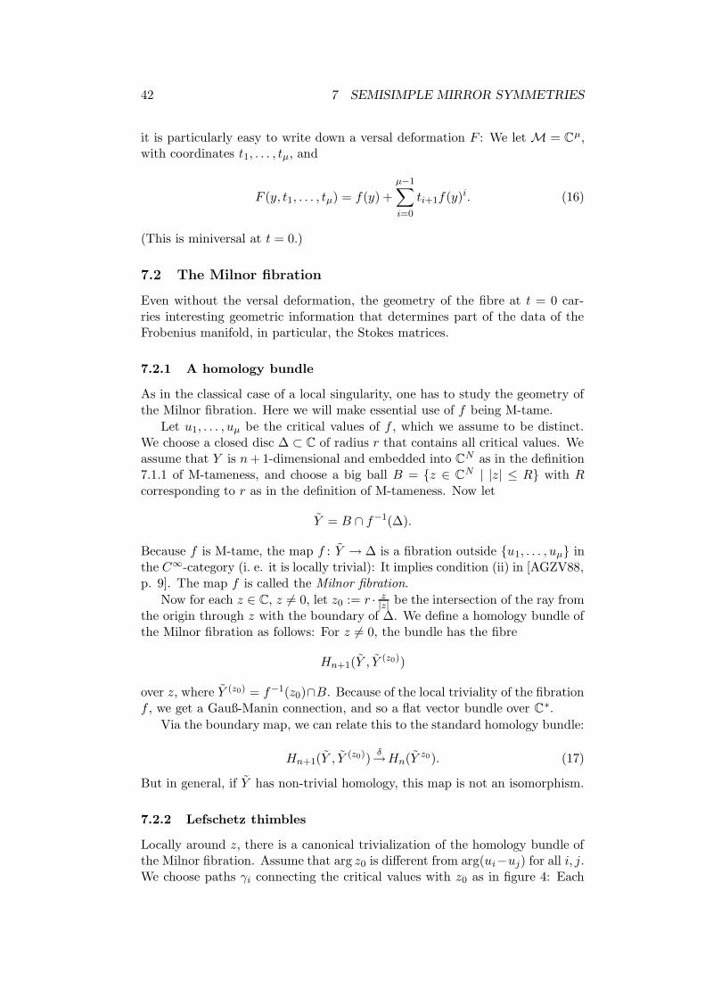
Locally around z, there is a canonical trivialization of the homology bundle ofthe Milnor fibration. Assume that arg z0 is different from arg(ui−uj) for all i, j.We choose paths γi connecting the critical values with z0 as in figure 4: Each
7.2 The Milnor fibration 43
path starts straight in the direction of arg z0, and then turns in to reach z0.5
Over each such path, we get a family of vanishing cycles that glue together toa real n+ 1-dimensional manifold Γi with boundary in Y (z0), called a Lefschetzthimble. (For a precise definition, we refer to [AGZV88] or the construction asexplicit manifolds below.) This gives canonical elements in Hn+1(Y , Y (z0)).
z_0
u_1
u_2
u_3
u_4
Figure 4: Paths underlying Lefschetz thimbles
We can extend this to a local trivialization by transforming the paths ho-motopically in ∆ \ u1, . . . un connecting the ui with z′0 for z′0 nearby z0. Ofcourse, as the homotopy classeses of the paths depend on the original choice ofz0, this does not yield a global trivialization.
We will also need the Lefschetz thimbles as explicit manifolds. For this,one has to choose a Riemannian metric g on Y . We then consider the gradientflow of the real Morse functions gz = Re(z−1f(·)) (i. e. the flow generated bythe vector field that is dual to the one-form dgz via the metric g). For eachcritical point of gz, we consider the unstable part of the Morse flow. This gives an+ 1-dimensional submanifold (by general Morse theory, and as Re(z−1f(·)) islocally of the form x2
1 + · · ·x2n+1−y2
1−· · · y2n+1 for suitable complex coordinates
zj = xj + iyj, i. e. for which z−1f = z21 + . . . z2
n+1; if the metric is given byg = dx2
1 + dy21 + · · · + dx2
n+1 + dy2n+1, the Lefschetz thimble is given by y1 =
· · · = yn+1 = 0, and the vanishing cycles are the level sets of this submanifold,i. e. given by the additional equation x2
1 + · · ·+ x2n+1 = t).
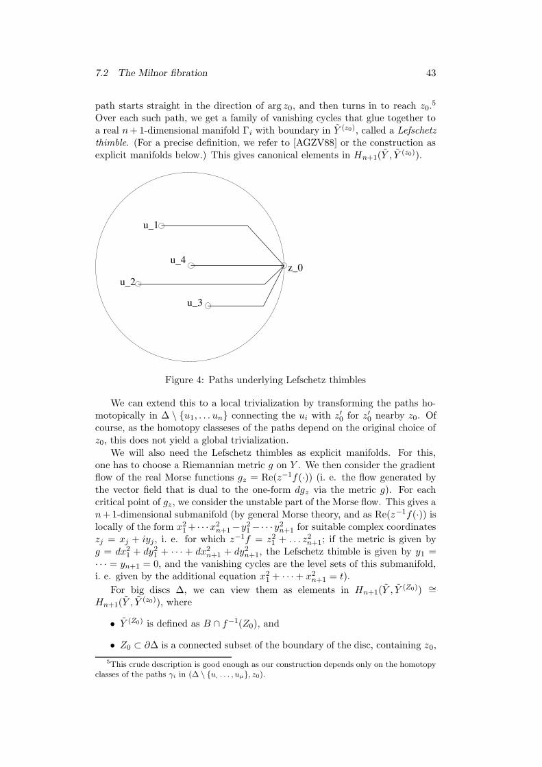
For big discs ∆, we can view them as elements in Hn+1(Y , Y (Z0)) ∼=Hn+1(Y , Y (z0)), where
• Y (Z0) is defined as B ∩ f−1(Z0), and
• Z0 ⊂ ∂∆ is a connected subset of the boundary of the disc, containing z0,
5This crude description is good enough as our construction depends only on the homotopyclasses of the paths γi in (∆ \ u, . . . , uµ, z0).
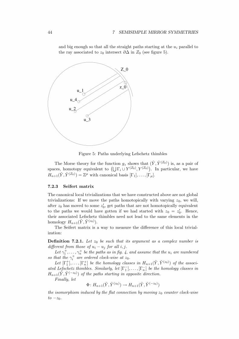
44 7 SEMISIMPLE MIRROR SYMMETRIES
and big enough so that all the straight paths starting at the ui parallel tothe ray associated to z0 intersect ∂∆ in Z0 (see figure 5).
u_1
u_2
u_4
u_3
z_0
Z_0
Figure 5: Paths underlying Lefschetz thimbles
The Morse theory for the function gz shows that (Y , Y (Z0)) is, as a pair ofspaces, homotopy equivalent to
(⋃Γi ∪ Y (Z0), Y (Z0)
). In particular, we have
Hn+1(Y , Y (Z0)) = Zµ with canonical basis [Γ1], . . . , [Γµ].
7.2.3 Seifert matrix
The canonical local trivializations that we have constructed above are not globaltrivializations: If we move the paths homotopically with varying z0, we will,after z0 has moved to some z′0, get paths that are not homotopically equivalentto the paths we would have gotten if we had started with z0 = z′0. Hence,their associated Lefschetz thimbles need not lead to the same elements in thehomology Hn+1(Y , Y (z0)).
The Seifert matrix is a way to measure the difference of this local trivial-ization:
Definition 7.2.1. Let z0 be such that its argument as a complex number isdifferent from those of ui − uj for all i, j.
Let γ+1 , . . . , γ
+n be the paths as in fig. 4, and assume that the ui are numbered
so that the γ+i are ordered clock-wise at z0.
Let [Γ+1 ], . . . , [Γ+
n ] be the homology classes in Hn+1(Y , Y (z0)) of the associ-ated Lefschetz thimbles. Similarly, let [Γ−1 ], . . . , [Γ−n ] be the homology classes inHn+1(Y , Y (−z0)) of the paths starting in opposite direction.
Finally, letΦ: Hn+1(Y , Y (z0))→ Hn+1(Y , Y (−z0))
the isomorphism induced by the flat connection by moving z0 counter clock-wiseto −z0.
7.3 The twisted de Rham-complex 45
The Seifert matrix Sij is the matrix representing the basis Φ([Γ+1 ]), . . .,
Φ([Γ+n ]) in terms of the basis [Γ−1 ], . . . , [Γ−n ] of Hn+1(Y , Y (−z0)).
So, similarly to the Stokes matrices, we can understand it as canonicallydefined Cech-cocycle. It is easy to prove that it is an upper triangular matrixwith ones on the diagonal.
7.3 The twisted de Rham-complex
Given a miniversal deformation of a singularity, the manifold germ M is au-tomatically equipped with a multiplication on the tangent sheaf. We simplypull back the ring structure of the Milnor ring via the Kodaira-Spencer isomor-phism (15).
We get two special vector fields onM: The Euler field E is the preimage ofFt ∈ OY×t/(TY (Ft) under this isomorphism, and the unit field e the preimageof the constant function 1.
So far the construction was canonical, i. e. it did not depend on choices.The multiplication satisfies an integrability condition, it is an F -manifold withEuler field as defined in [HM99].
Constructing the flat metric of the Frobenius manifold is more involved andit depends on choices. Also, it is not known to work in complete generality. Wewill not try to outline the full construction of the Frobenius manifold. Instead,we will describe only as much as we need to define its Stokes matrices.
We will from here on work in the algebraic category, that is Y is an smoothaffine scheme of finite type over C, with structure sheaf OY , and f ∈ OY (Y ).As we are working with a globally defined function f instead of just a functiongerm, there is a problem with “singularities coming from infinity”. Again, thiscan be seen very explicitly in the case of tame semisimplicity:
Consider the Milnor ring of the deformed function Ft as defined by (16): Itis defined by the ideal generated by
(dY Ft)(y) =
(1 +
µ−1∑
i=1
itif(y)i−1
)(dY f)(y).
We have a common zero of these functions iff dY f = 0 or f(y) is a solution of
p(λ) = 1 +
µ−1∑
i=1
itiλi−1.
These solutions go to infinity if the ti go to zero.
However, since we are assuming tame simplicity at t = 0, we do not needthe versal deformation at all to define Stokes matrices. The fibre at t = 0 issufficient.
Definition 7.3.1. The twisted relative algebraic de Rham complex associated
to the function f is the complex of sheaves Ω•Y [z, z−1] · e−fz on C × Y withdifferential df = z · dY . (Here z is the coordinate on C.)
46 7 SEMISIMPLE MIRROR SYMMETRIES
A q-form in this complex is given as ω =∑
i ωizi · e−fz , with ωi a relative
q-form, given in coordinates y1, . . . , yn on Y as ωi =∑gJ(y)dyj1 ∧ · · · ∧ dyjq .
Algebraic means that gJ is a polynomial function on Y . Its differential is
df (ω · e−fz ) = (z dY ω − df ∧ ω) · e−fz .
The definition of this complex might look a little unmotivated. By [DS02a,section 2.c], this complex is a representative for the Fourier dual of the deRham-complex of f , in a D-module sense.
Let π : C∗ × Y → C∗ be the projection. The sheaves π∗(
Ω•Y [z, z−1] · e−fz)
are equipped with a meromorphic connection:
∇∂z(ω · e−fz
)=
(∂ω
∂z+f
z2ω
)e−fz (18)
The formula
∇∂zdf(ω · e−fz
)= df
(−ωz· e−fz +∇∂z
(ω · e−fz
))
shows that ∇∂z induces a connection on Hn+1(π∗Ω•Y [z, z−1] · e−fz
). One mo-
tivation behind this definition is to make the pairing in equation (19) flat.
Proposition 7.3.2. [DS02a] The cohomology sheaf Hn+1(π∗Ω•Y [z, z−1] · e−fz
)
of the twisted de Rham complex in degree n+ 1 is locally free of rank µ.
Crucial for Stokes matrices is now the extension of Hn+1 to a free sheaf atz = 0:
Definition 7.3.3. The Brieskorn lattice H0 is the image of the natural map
Ωn+1[z] → Hn+1 = Ωn+1[z, z−1]/((zdY − df∧)Ωn[z, z−1]
).
Proposition 7.3.4. [DS02a] The Brieskorn lattice is a locally free sheaf of rankµ on C, with a natural isomorphism H0/zH0
∼= Ωn+1/ (df ∧ Ωn).
The Stokes matrix of the Frobenius manifold is the Stokes matrix of thedifferential module H0 (after base change to C(z)).
7.4 Frobenius manifold mirror symmetry
To construct a Frobenius manifold, one has to extend this connection in twoways: First, one has to extend it to a connection onM×C, whereM is the basespace of the versal deformation F above. Secondly, one has to solve a Riemann-Hilbert-Birkhoff problem, and extend it to a flat connection on a globally freesheaf F on M× P1.
Finally, one has to find a primitive form that produces an isomorphismfrom TM to the sheaf p∗F of fibrewise global sections of F . Generally, neitherexistence nor uniqueness of such a primitive form is clear. We refer to [Her03]

7.5 Relating Stokes and Seifert matrix 47
for an overview of the whole construction, and to [DS02a] and [DS02b] andreferences therein for details.
It is generally believed that this construction produces mirror partners forgenerically semisimple quantum cohomology of Fano varieties. This has beenproven for projective spaces:
Theorem 7.4.1. [Bar01] Let Y be the submanifold of Cn+1 given byX0X1 · · ·Xn = 1, and let f = X0 + · · · + Xn. We use the deformationF : Y × Cn+1 → C of f given by F = f +
∑i aif
i (where ai are the coordi-nates on Cn+1).
For an appropriate choice of the metric, the Frobenius manifold associated tothis deformation space is isomorphic to the Frobenius manifold of the quantumcohomology of Pn.
7.5 Relating Stokes and Seifert matrix
Let us abbreviate the sheaves defined in sections 7.2 and 7.3 with Hn+1 =
Hn+1(Y , Y z0) and Hn+1 = Hn+1(π∗Ω•Y [z, z−1] · e−fz ). We can define a pairingbetween the two fibres Hn+1|z and Hn+1|z′ for any pair of non-zero complexnumber z, z′ with Re
(zz′)> 0. It is sufficient to define it for a representative
ω · e−fz and the class of a Lefschetz thimble [Γ].
Extend the path γ : [0, 1]→ C as in fig. 5 to a straight path γ∞ : [0,∞[→ Cgoing to infinity, and accordingly extend the Lefschetz thimble to Γ∞. We set
⟨ω · e−fz , [Γ]
⟩=
∫
Γ∞ω · e−fz . (19)
Proposition 7.5.1. Equation (19) gives a well-defined pairing that is flat withrespect to the Gauß-Manin connection on the right-hand-side and the connectionas defined in (18) on the left-hand side.
Proof. Outside f−1(u1, . . . , uµ), we can write ω in the form ω = df ∧ φ,where φ is a n− 1-form. For any z ′ 6= ui, we have
φ|f−1(z′) = Resf−1(z′)(ω).
This allows us to rewrite the integral as
∫
Γ∞ω · e−fz =
∫
γ∞dτ · e−τz
∫
Γτ
φ.
We have written Γτ = Γ ∩ f−1(τ) for the vanishing cycle in the fibre over τbelonging to Γ.
From the results in [Pha83], it follows that the Gauß-Manin system of func-tions obtained as
∫Γτφ has a regular singularity at τ =∞. In particular, these
functions are of moderate growth. This is essential for all calculations.
Due to Re(zz′)> 0, the term e
−τz will be rapidly vanishing as τ goes to
infinity. Hence the integral converges.

48 7 SEMISIMPLE MIRROR SYMMETRIES
Now if ω · e−fz is of the form df (ω′ · e−fz ) = zd(ω′ · e−fz ) for some algebraicn− 1-form ω′, we can by Stokes’ theorem conclude for finite t ∈ R:
∫
γ|[0,t]dτ · e−τz
∫
Γτ
φ = ze−γ(t)z
∫
Γγ(t)
ω′.
This goes to zero with t→∞.With similar arguments, one can show that it is flat with respect to the
Gauß-Manin connection on Hn+1. The flatness with respect to the connectionin (18) is immediate. 2
From proposition 7.3.4, it is clear that z2∇ ∂∂z
operates on H0/zH0 as a
diagonal matrix with entries (u1, . . . , uµ). Further, for z → 0, all the integralsover Lefschetz thimbles become dominated by the behaviour at the criticalpoint, and so the result is dominated by a term e
uiz . This motivates some of
the following statements.
Conjecture 7.5.2. • The pairing (19) is non-degenerate.
• After base change to C((z)), the pair (H0,∇) becomes isomorphic as adifferential module to the direct sum of the differential equations δ− ui
z —where we have reintroduced the notation of section 5.2. Let ωi ∈ H0⊗C[z]
C((z)) be the elements defining this isomorphism.
• Fix some z′ 6= 0, and fix an i, 1 ≤ i ≤ µ. Let H be the half planeof complex numbers z with Re z
z′ > 0. Let H0(i) be the subsheaf of H0|Hdefined by 〈H0(i), [Γj ]〉 = 0 for all j 6= 0. By the preceding proposition andthe first part of the conjecture, this defines a one-dimensional differentialsubmodule of (H0,∇).
• In the isomorphism H0/zH0∼= Ωn+1/ (df ∧ Ωn), the submodule
H0(i)/zH0(i) corresponds to the part concentrated at the critical pointover ui on the right hand side.
• Let (φi(z))i ∈ Hn+1|z be the dual basis to the basis ([Γi])i of Hn+1|z′ in our
pairing. We define ωi(z) by ωi(z) · e−fz = φi(z) · e
−uiz . The conjecture is
that ωi(z)e−fz is an element in H0(i)⊗(Cz)A6 that has ωi as asymptotic
expansion. (Notice that, since φi is flat, the section ωi(z)e−fz is a solution
to the differential equation δ − uiz .)
Since we can vary z′ a little without changing the homology classes of the Γi,we can in fact define H0(i) and ωi on a sector slightly larger than a half-plane.If we do the same for −z′ instead of z′, we get analogously sections ω−i on asector covering the opposite half plane. We use this sectors as the covering U1
and U2 needed to define the Stokes matrices of the connection.
Corollary 7.5.3. The Stokes matrix of (H0,∇) with respect to (U1, U2) is thetranspose of the Seifert matrix of f (where we chose z0 in definition 7.2.1 asz0 = z′).
6See 5.2.5 for the definition of A.
7.6 Homological mirror symmetry and exceptional systems 49
Proof. The intersection U1 ∩ U2 has two components, and we chose z ar-bitrary in the component that we meet when we go counter-clockwise starting
from z′. The Stokes matrix is the matrix expressing the basis (ω−i (z) · e−uiz )i of
Hn+1|z in terms of the basis (ωi(z) ·e−uiz )i. The first is the dual basis to
([Γ−i ]
)i
of Hn+1|z, the latter to ([Γi])i. Here we have identified Hn+1|z′ ∼= Hn+1|−z′ ∼=Hn+1|z via the flat Gauß-Manin connection.
The Seifert matrix expresses the basis ([Γi])i in terms of the basis([Γ−i ]
)i;
it is thus clear that it coincides with the Stokes matrix. 2
7.6 Homological mirror symmetry and exceptional systems
In his talk at the Berkeley ICM 1994 [Kon95], Kontsevich proposed a new mirrorsymmetry conjecture. According to it, the bounded derived category Db(X)of coherent sheaves on X should be equivalent to the derived Fukaya categoryassociated to the mirror partner Y .
In the case of Calabi-Yau varieties, this Fukaya category is reasonably well-defined. For our purposes, however, we will need a Fukaya category associatedto the mirror F : Y ×M→ C. We will assume that F is the deformation of afunction f : Y → C that has only A1-singularities.
However, apparently no one has yet succeeded in a geometric definition ofthis Fukaya category. Still, we can see how some aspects of the Fukaya categoryfit into the mirror picture with Fano varieties, as we will describe below.
The objects of the Fukaya category on a Calabi-Yau variety are (graded)Lagrangian submanifolds Λ ⊂ Y equipped with a flat U(n)-bundle U on Λ.Graded Lagrangian submanifold means the following: Let p : L → Y be the La-grangian Grassmannian of the tangent bundle of Y . Let p : L → Y be the bundlewhich has as fibres the universal covers of the fibres of p. A Lagrangian sub-manifold automatically induces a section s : Λ→ p−1(Λ). A graded Lagrangiansubmanifold comes with a lift s of s to the universal cover: s : Λ→ p−1(Λ).
It is suggested to either restrict the objects to be special Lagrangian subman-ifolds, or to take equivalence classes of Lagrangian manifolds under Hamiltoniandeformations.
The morphisms in the Fukaya category are complexes. Let (Λ1, U1) and(Λ2, U2) be two graded Lagrangian submanifolds with flat U(n)-bundles. Weassume that the two submanifolds intersect transversely; otherwise the defini-tion of the Hom-complexes is unclear (at least in full generality). Let xi bethe intersection points of Λ1 and Λ2. If we compare s1 and s2 at an intersec-tion point xi, we get a path in the Lagrangian Grassmannian of TxiY . TheMaslov index (or rather one of the many versions of Maslov indices) associatesan integer µ(xi) to such a path. Now Hom•(Λ1,Λ2) is a complex with objects
Homk(Λ1,Λ2) =⊕
xi:µ(xi)=k
Hom(U1|xi , U2|xi).
We don’t need to know the precise definition of the Maslov index7, all we
7If γ : [0, 1] → GrL(V ) is a path in the Lagrangian Grassmanian of a symplectic vector
50 7 SEMISIMPLE MIRROR SYMMETRIES
need is that (−1)µ(xi) is the local intersection multiplicity of Λ1 and Λ2 at xi.8
From this, it follows immediately that
χ(Hom•(Λ1,Λ2)) = Λ1 · Λ2. (20)
The following conjecture is probably believed by many people:
Conjecture 7.6.1.
The Fukaya category associated to a mirror construction as in section 7.1 hasa full exceptional system (E1, . . . , Eµ). The underlying manifolds of the excep-tional objects can be chosen to be Lefschetz thimbles (Λ1, . . . ,Λµ) of the functionf . In analogy to equation (20), we have
χ(Hom•(Ei, Ej)) = Sij
for i < j, with S being the Seifert matrix.
This seems more a conjecture about the correct definition of the Fukayacategory than anything else. We should explain the analogy to equation (20) abit: In the case where the boundary map (17) is an isomorphism, and where nis even, the entries Sij can be reconstructed via Picard-Lefschetz theory fromthe intersection pairing in Hn(Y z0). But in general, we are not aware of aninterpretation of Sij as an intersection product.
Physicists seem to have understood this part much better. In fact, themost compelling evidence for the conjecture seems that it would be the bestmathematical translation of the work of Hori, Iqbal and Vafa in [HIV00]. Thenumbers Sij are soliton numbers in their framework.
7.7 Putting it together
We can now explain claim 2 of Dubrovin’s conjecture 6.2.1 in a few sentences:Let S be the Stokes matrix of a semisimple Frobenius manifold coming fromthe quantum cohomology of a variety X. By a combinatorial mirror symmetrystatement such as 7.4.1, the underlying Frobenius manifold is isomorphic toone obtained from a mirror construction starting with a pair (Y, f) as in thissection. By 7.5.3, this is the same as the Seifert matrix. By 7.6.1, it coincideswith the Stokes matrix of the Fukaya category associated to (Y, f). And ifKontsevich’s categorical mirror symmetry holds, this is then also the Stokesmatrix of Db(X).
Needless to say, this is a very conjectural explanation.
space V such that γ(1) is transversal to γ(0), then this integer is roughly defined as follows:Let Γ ⊂ GrL be the cycle whose support are those subspaces that do not intersect thesubspace γ(0) transversally. This is called the Maslov cycle of γ(0). The Maslov index countsthe number of intersection points of γ([0, 1]) with the cycle Γ with multiplicities. The onlyambiguity left is at the point γ(0); one possible solution is to extend the path γ in a sufficientlyuniform manner to a path γ : [−ε, 1]→ GrL.
8If we have chosen an orientation of Λ1, then we can choose a compatible orientation of Λ2
by comparing s1 and s2 at any intersection point.
51
8 Blow-ups
8.1 Complete exceptional system and blow-ups
The following theorem produces further examples of varieties that have an ex-ceptional system:
Theorem 8.1.1. [Orl92] Let Y be a smooth subvariety of the smooth projectivevariety X. Let ρ : X → X be the blow-up of X along Y .
If both Y and X have an exceptional system, then the same is true for X.
We will only be interested in the case where Y is a point. In this case, theexceptional collection on X is easy to construct: Let Pn−1 ∼= E ⊂ X be theexceptional divisor (n is the dimension of X). If E0, . . . , Er is a given exceptionalsystem in Db(X), then OE(−n+ 1), . . . ,OE(−2),OE(−1), ρ∗(E0), . . . , ρ∗(Er) isan exceptional system in Db(X).
The construction in the general case is similar. Let ρY : Y → Y be theexceptional divisor, which is a projective bundle. If E is an exceptional objectin Db(Y ), then ρ∗Y (E) ⊗ OY (−i) is an exceptional object in Db(Y ). Theseobjects play the role of OE(−i) above.
8.2 Semisimplicity and blow-ups
So let us now assume that the variety X satisfies Dubrovin’s conjecture, i. e.that it has both a complete exceptional collection and semisimple quantumcohomology. Let Xr be its blow-up at r points. By Theorem 8.1.1, this a testfor Dubrovin’s conjecture: We already know that Xr has an exceptional system,so we would like to show that it has semisimple quantum cohomology as well.
Under specific additional assumptions, this is done by the following theorem:
Theorem 8.2.1. Let Xr → X be the blow-up of a smooth projective variety Xat r points. Assume that X is convex (so that all the moduli spaces M g,n(X,β)are smooth of expected dimension).
If the quantum cohomology of X has a semisimple point in H 2(X) over theNovikov ring, then the same is true for Xr.
In the case of dimension two, Del Pezzo surfaces were treated in [BM01],where the results of [GP98] on their quantum cohomology were used. Thegeneralization presented here uses instead the results in Andreas Gathmann’spaper [Gat01]. The essential idea is a variant of the idea used in [BM01]:a partial compactification of the spectral cover map where the exponentiatedcoordinate of an exceptional class vanishes. However, in our case, this is onlypossible after base change to a finite cover of the spectral cover map.
The assumption that semisimple points can already be found in H 2 (in thesmall quantum cohomology) is not a completely arbitrary one. It induces aReconstruction Theorem, which states that all Gromov-Witten invariants canbe reconstructed from four point correlators (see [BM01, Theorem 1.8.3] for aprecise statement). As for the convexity, we refer to the discussion below.
52 8 BLOW-UPS
8.2.1 Gathmann’s results
The following theorem collects the results of [Gat01] that we will need later.The essential results for the proof in the next section will be part 1a and 2b.
Theorem 8.2.2. Let X → X be the blow-up of a smooth projective varietyX of dimension n at r points x1, . . . , xr. Let Ei be the exceptional divisorcooresponding to xi, and with the same letter we will denote the exceptionalclass in H2(X). Let E′i ∈ H2(X) be the exceptional homology class of a line inEi ∼= Pn−1.
The following assertions relate the Gromov-Witten invariants of X to thoseof X (which we will denote by 〈. . . 〉Xβ and 〈. . . 〉Xβ , respectively):
1. (a) If X is convex, the following holds:
Let β ∈ H2(X) be any non-exceptional homology class—so β isany element of H2(X)—, and let T1, . . . , Tm be any number of non-exceptional classes in H∗(X), which we can identify with their preim-ages in H∗(X). Then it does not matter whether we compute thefollowing Gromov-Witten invariants with respect to X or X:
〈T1 ⊗ · · · ⊗ Tm〉Xβ = 〈T1 ⊗ · · · ⊗ Tm〉Xβ . (21)
(b) Consider the Gromov-Witten invariants 〈T1⊗· · ·⊗Tm〉Xβ with β beingpurely exceptional, i. e. β = d ·E ′i.If any of the cohomology classes T1, . . . , Tm are non-exceptional, theinvariant is zero. All invariants involving only exceptional cohomol-ogy classes can be computed recursively from the following:
〈En−1i ⊗En−1
i 〉XE′i = 1. (22)
They depend only on n.
2. If either X is convex, or part 1a is true for other reasons, the followingstatements hold:
(a) Using the associativity relations, it is possible to compute all Gromov-Witten invariants of X from those mentioned above in 1a and 1b.9
(b) Vanishing of mixed classes: Write β ′ ∈ H2(X) in the form β ′ =β + d · E′i where β is the non-exceptional part with respect to Ei;assume that β 6= 0. Let T1, . . . Tm be non-exceptional cohomologyclasses with respect to Ei. Let l be a non-negative integer, and let2 ≤ k1, . . . , kl ≤ n− 1 be integers satisfying
(k1 − 1) + · · ·+ (kl − 1) < (d+ 1)(n− 1).
Unless we have both d ≤ 0 and l = 0, this implies the vanishing of
〈T1 ⊗ · · · ⊗ Tm ⊗Ek1i ⊗ · · · ⊗E
kli 〉β = 0.
9We will make this more precise later on.
8.2 Semisimplicity and blow-ups 53
Proof. All equations follow trivially from statements from lemma 2.2, lemma2.4 and proposition 3.1 in [Gat01]. Note that we have made explicit the remark2.3 of Gathmann’s paper: the only part where Gathmann uses the convexity ofX is in the proof of equation (21). So if it can be proven by other means, theassumption of convexity of X can be dropped. 10
The only apparent change to Gathmann’s statements is in 2b: We onlyassume that β 6= 0, whereas Gathmann assumes that β is not purely exceptional.But the missing cases are treated by [Gat01, lemma 2.4, (i)]. 2
We want to apply Gathmann’s theorems to the map Xr → Xr−1, whereXr and Xr−1 are the blow-up of a convex variety X at r and r − 1 points,respectively; but we do not want to assume the convexity of Xr−1. So we needto prove equation (21). We will use Gathmann’s algorithm to compute theGromov-Witten invariants of Xr−1 and Xr from those of X (i. e. we applyGathmann’s theorems to the maps Xr → X and Xr−1 → X).
We want to show that his algorithm gives the same number for Gromov-Witten invariants of Xr−1 and the non-exceptional Gromov-Witten invariantsof Xr. First, we need to introduce some of his notations.
Definition 8.2.3. Denote by V a smooth projective variety. Let β ∈ H2(V )be an effective homology class, and let T1, . . . , Tm, µ1, µ2, µ3, µ4 ∈ H∗(V ) becohomology classes. Write T for T = T1 ⊗ T2 ⊗ · · · ⊗ Tm. Let ∆0, . . . ,∆q be abasis of the cohomology.
By Eβ(T ;µ1, µ2 | µ3, µ4) we denote the equation11
0=〈T ⊗ µ1 ⊗ µ2 ⊗ µ3 · µ4〉β + 〈T ⊗ µ3 ⊗ µ4 ⊗ µ1 · µ2〉β−〈T ⊗ µ1 ⊗ µ3 ⊗ µ2 · µ4〉β − 〈T ⊗ µ2 ⊗ µ4 ⊗ µ1 · µ3〉β+∑β1,β2
∑T1,T2
∑i,j
(∆i,∆j)(〈T1 ⊗ µ1 ⊗ µ2 ⊗∆i〉β1〈T2 ⊗ µ3 ⊗ µ4 ⊗∆j〉β2
−〈T1 ⊗ µ1 ⊗ µ3 ⊗∆i〉β1〈T2 ⊗ µ2 ⊗ µ4 ⊗∆j〉β2
)
Here the sums go over
• all decompositions of β as a sum β = β1 +β2 of effective homology classes,
• decompositions of T = T1 ⊗ T2 that come from decompositions ofT1, . . . , Tm into two sets, and
• all 0 ≤ i, j ≤ q.
This equation is guaranteed to hold by the axioms for Gromov-Witten in-variants and is necessary for associativity.
We can now describe Gathmann’s recursive algorithm:
10 The author is convinced that equation (21) is always true. However, a proof is technicallyhighly inconvenient in the framework of the construction of the virtual fundamental classesin [Beh97]: The natural morphism M0,n(X, β) → M0,n(X, β) does not commute with themorphism to M(0, n) (the moduli space of prestable curves), with respect to which the perfectrelative obstruction theory is constructed. This makes it hard to compare the relative virtualnormal cones.
If the virtual fundamental class could be constructed via an absolute obstruction theory(using the non-relative virtual normal cone of [BF97]), a proof of equation (21) might be easy.
11We write µi · µj for the cup product, and (∆i,∆j) for the Poincare pairing.
54 8 BLOW-UPS
Theorem 8.2.4. Given a blow-up X of a convex variety X at a finite numberof points, we can compute all Gromov-Witten invariants of X recursively, usingthe associativity relations, from those determined by 8.2.2, 1a and 1b, in thefollowing way:
By linearity, we can assume that all cohomology classes are of pure dimen-sion and either non-exceptional or purely exceptional. Write T = T1⊗ . . . Tm′⊗Tm′+1 ⊗ · · · ⊗ Tm with T1, . . . , Tm′ non-exceptional, and Tm′+1, . . . , Tm excep-tional. By the divisor axiom, we can assume without loss of generality thatnone of the exceptional cohomology classes are divisorial, and that the sum ofthe codimensions of T1, . . . , Tm′ is at least n+ 1.12 In particular, m′ is at least2. Also, we assume codimT1 ≥ codimT2 ≥ · · · ≥ codimTm′ .
Then we proceed as follows:
(A) If m′ < m, then Tm = Eki for some exceptional divisor class Ei. We thenuse
Eβ(T ′;T1, T2 | Ei, Ek−1i ) with T ′ = T3 ⊗ · · · ⊗ Tm−1
(B) If m′ = m, T1 = [pt] and codim T2 ≥ 2, we choose µ, ν such that µ isdivisorial, codim ν = n− 1 and µ · ν = [pt], and we choose an exceptionaldivisor Ei with Ei·β 6= 0 (such an Ei must exist, as otherwise the invariantwould be determined by equation (21)).
We use
Eβ(T ′;µ, ν | Ei, T2) with T ′ = T3 ⊗ · · · ⊗ Tm
(C) In all other cases (i. e. m′ = m, but not case (B)) we again choose an Eias in the previous case. We use the equation
Eβ+E′i(T ′;T1, T2 | Ei, En−1
i ) with T ′ = T3 ⊗ · · · ⊗ Tm
Here “using equation Eβ(. . . )” means
• that there is a partial ordering on the set of pairs (β, T ),13
• that this ordering does not have infinite descending chains, and
• that at each step, the respective equation (together with the divisor axiom)determines the correlator in question uniquely from correlators that aresmaller with respect to the partial ordering.
Proposition 8.2.5. Let β ∈ H2(Xr−1) and T1, . . . , Tm ∈ H∗(Xr−1) be(co-)homology classes in Xr−1, and identify them with their images in the(co-)homology of H∗(Xr).
If we compute 〈T1 ⊗ · · · ⊗ Tm〉Xr−1
β and 〈T1 ⊗ · · · ⊗ Tm〉Xrβ according totheorem 8.2.4, we can make corresponding choices at each step, and get anequivalent recursion; thus, the two values coincide. Therefore, Theorem 8.2.2holds for the map Xr → Xr−1.
12Otherwise, we can enlarge the list of the Ti by any number of divisors D with (D, β) 6= 0.13Its precise definition is not relevant for us, so we will not repeat it here.

8.2 Semisimplicity and blow-ups 55
Proof. The “initial values” of the algorithm, i. e. the non-exceptional in-variants of X, and the purely exceptional ones, are identical in both cases byTheorem 8.2.2, 1b and 1a.
We assume that Xr and Xr−1 are the blow-up of X at x1, . . . , xr, andx1, . . . , xr−1, respectively. Having chosen a basis ∆0, . . . ,∆q′ of H∗(Xr−1), weextend this to a basis ∆0, . . . ,∆q of H∗(Xr) by identifying ∆0, . . . ,∆q′ withtheir images in H∗(Xr), and setting ∆q′+k = Ekr for 1 ≤ k ≤ n− 1.
Now at each recursion step, we make the necessary choices in H ∗(Xr−1),and then make the corresponding choice via the inclusion H ∗(Xr−1) ⊂ H∗(Xr)for Xr.
Let us assume that the claim has already been proven for all smaller classesin Gathmann’s partial ordering of pairs (β, T ).
Consider case (A) of the algorithm. In Xr, the equation to be used readsas:
0=〈T ′ ⊗ T1 ⊗ T2 ⊗Ei ·Ek−1i 〉Xrβ + 〈T ′ ⊗Ei ⊗Ek−1
i ⊗ T1 · T2〉Xrβ + 0 + 0
+∑
T1,2,β1,2,i,j
(∆i,∆j)(〈T1 ⊗ T1 ⊗ T2 ⊗∆i〉Xrβ1
〈T2 ⊗Ei ⊗Ek−1i ⊗∆j〉Xrβ2
−〈T1 ⊗ T1 ⊗Ei ⊗∆i〉Xrβ1〈T2 ⊗ T2 ⊗Ek−1
i ⊗∆j〉Xrβ2
)
(Here we have abbreviated the big sum of 8.2.3. The third and fourth summandthere are zero because of Ei · T1 = Ei · T2 = 0.)
The first summand is the one we want to compute. The second summandis identical to 〈T ′ ⊗Ei ⊗Ek−1
i ⊗ T1 · T2〉Xr−1
β by induction hypothesis.All summands in the big sum can, by induction hypothesis, be assumed to
be identical to the corresponding terms 〈· · · 〉Xr−1 in the corresponding equationin Xr−1—if they appear in that equation at all. The summands that do notappear in the corresponding equation for Xr−1 come from
1. decompositions of β = β1 + β2 that are non-trivial with respect to theexceptional divisor Er, i. e. β1 = β′1 + d ·E′r, β′2 = β′2 − d ·E′r with d > 0,and/or
2. the ∆i,j being elements of the basis of H∗(Xr) that do not appear in thebasis of H∗(Xr−1), i. e. ∆i,j = Ekr .
If we are in case 2, but not in case 1, both invariants 〈· · · 〉Xrβ1,2vanish by 8.2.2, 2b
(with d = 0 and l = 1). In the case 1, the correlator 〈· · · 〉Xrβ1vanishes, this time
by 8.2.2, 2b with d > 0 and l ≤ 1.Cases (B) and (C) are completely analogous. 2
8.2.2 Proof of Theorem 8.2.1
Proof.[of Theorem 8.2.1] By induction we only need to treat the case of theblow-up of a single point.
We consider the spectral cover map restricted to H 2(Xr), over the Novikovring. Let Nr and Nr−1 be the Novikov ring of Xr and Xr−1, respectively. Letβ1, . . . , βs be a basis of H2(Xr−1), and let E ′ = E′r be the line in the exceptionaldivisor of Xr → Xr−1. Write qi = qβi and Q = q−E
′for the corresponding
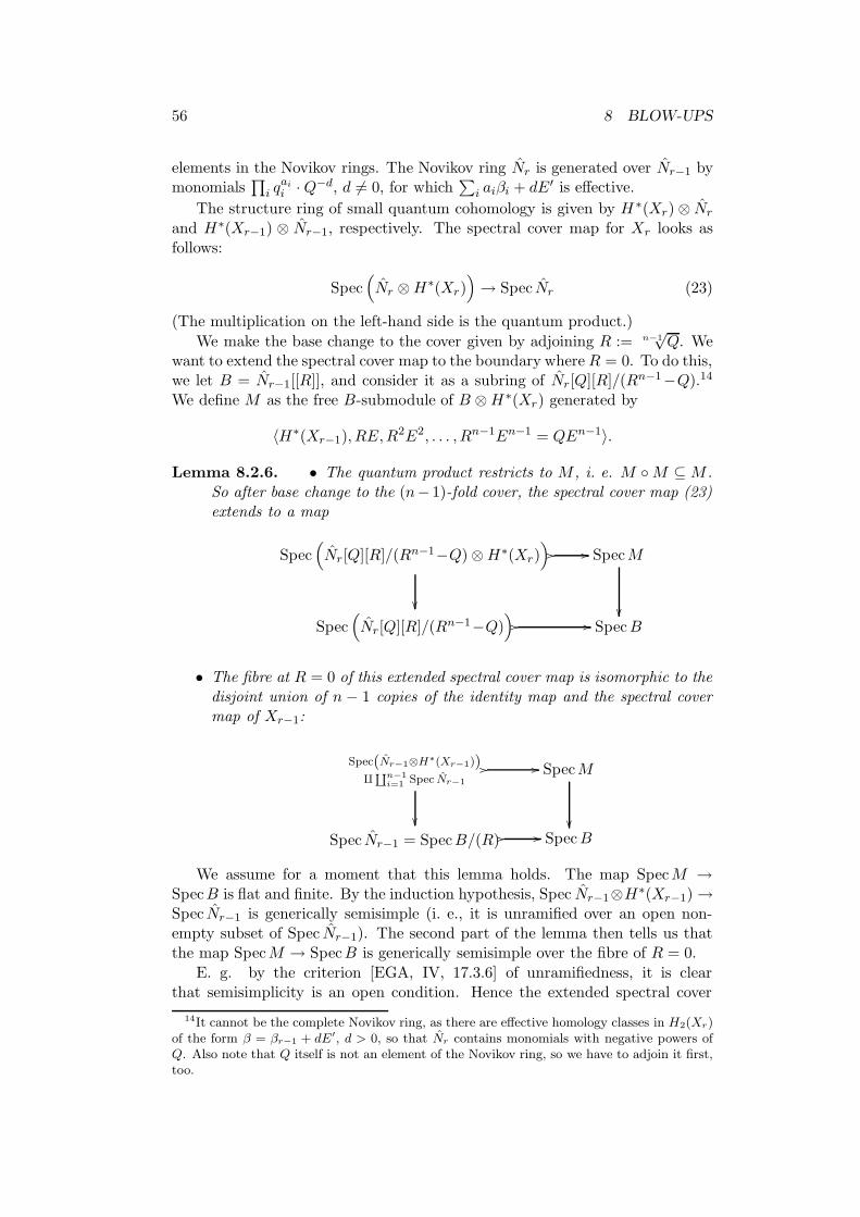
56 8 BLOW-UPS
elements in the Novikov rings. The Novikov ring Nr is generated over Nr−1 bymonomials
∏i qaii ·Q−d, d 6= 0, for which
∑i aiβi + dE′ is effective.
The structure ring of small quantum cohomology is given by H ∗(Xr)⊗ Nr
and H∗(Xr−1) ⊗ Nr−1, respectively. The spectral cover map for Xr looks asfollows:
Spec(Nr ⊗H∗(Xr)
)→ Spec Nr (23)
(The multiplication on the left-hand side is the quantum product.)
We make the base change to the cover given by adjoining R := n−1√Q. We
want to extend the spectral cover map to the boundary where R = 0. To do this,we let B = Nr−1[[R]], and consider it as a subring of Nr[Q][R]/(Rn−1−Q).14
We define M as the free B-submodule of B ⊗H∗(Xr) generated by
〈H∗(Xr−1), RE,R2E2, . . . , Rn−1En−1 = QEn−1〉.
Lemma 8.2.6. • The quantum product restricts to M , i. e. M M ⊆M .So after base change to the (n− 1)-fold cover, the spectral cover map (23)extends to a map
Spec(Nr[Q][R]/(Rn−1−Q)⊗H∗(Xr)
)
// // SpecM
Spec
(Nr[Q][R]/(Rn−1−Q)
)// // SpecB
• The fibre at R = 0 of this extended spectral cover map is isomorphic to thedisjoint union of n− 1 copies of the identity map and the spectral covermap of Xr−1:
Spec(Nr−1⊗H∗(Xr−1))q‘n−1
i=1 Spec Nr−1
// //
SpecM
Spec Nr−1 = SpecB/(R) // // SpecB
We assume for a moment that this lemma holds. The map SpecM →SpecB is flat and finite. By the induction hypothesis, Spec Nr−1⊗H∗(Xr−1)→Spec Nr−1 is generically semisimple (i. e., it is unramified over an open non-empty subset of Spec Nr−1). The second part of the lemma then tells us thatthe map SpecM → SpecB is generically semisimple over the fibre of R = 0.
E. g. by the criterion [EGA, IV, 17.3.6] of unramifiedness, it is clearthat semisimplicity is an open condition. Hence the extended spectral cover
14It cannot be the complete Novikov ring, as there are effective homology classes in H2(Xr)of the form β = βr−1 + dE′, d > 0, so that Nr contains monomials with negative powers ofQ. Also note that Q itself is not an element of the Novikov ring, so we have to adjoin it first,too.
8.2 Semisimplicity and blow-ups 57
map is generically semisimple. The same must then hold for the map overNr[Q][R]/(Rn−1−Q), and, as unramifiedness can be checked after a base changeto a covering, the original spectral cover map (23). 2
Proof.[of the lemma] Both claims follow from a close investigation of allpossible products, using mainly Gathmann’s vanishing result.
Let ∆0, . . . ,∆m be a graded basis of H∗(Xr−1), which is an extension ofthe basis ∆1, . . . ,∆s of H2(Xr−1) that we chose above, and which contains ∆0
as the unit and ∆m as the dual class of a point. The matrix of the Poincarepairing with respect to this basis has entries gij .
The following formulas compute quantum products up to higher orders ofR. We denote the product taken in the quantum cohomology of Xr and Xr−1
by Xr and Xr−1 , respectively. We write β as β = βr−1 + d · E′ with βr−1 ∈H2(Xr−1) as the non-exceptional part. The references “no. 1a” etc. alwayspoint to the parts of Theorem 8.2.2.
We claim:
∆i Xr ∆j =∑
k,l
∑
β
〈∆i∆j∆k〉βgkl∆l ·Q−ds∏
ν=1
q(β,∆ν)v
+(−1)n−1n−1∑
k=1
∑
β
〈∆i∆jEk〉βEn−k ·Q−d
s∏
ν=1
q(β,∆ν)v
= ∆i Xr−1 ∆j +O(Q) (24)
To show this equality we need to examine three cases according to β:
• If d = 0, then the contribution to the second sum vanishes by no. 2b.By no. 1a, the first sum restricted to the cases d = 0 computes exactly∆i Xr−1 ∆j .
• The term O(Q) covers all summands with d < 0.
• If d > 0, all relevant Gromov-Witten invariants appearing in equation(24) vanish by no. 2b (respectively by no. 1b in the case βr−1 = 0).
For the next product that we have to examine (where i, j > 0), we get:
∆i Xr RjEj =∑
k,l
∑
β
〈∆iEj∆k〉βgkl∆l · RjQ−d
s∏
ν=1
q(β,∆ν)v
+(−1)n−1∑
k
∑
β
〈∆iEjEk〉βEn−k ·RjQ−d
s∏
ν=1
q(β,∆ν)v
= O(R ·M) (25)
Again we have to treat the three different cases:
• If d = 0, then the contribution to the first sum vanishes by no. 2b. Thevanishing result also implies that 〈∆iE
jEk〉β can only be non-zero if j +k − 2 ≥ n− 1, i. e. j ≥ n− k + 1. Then RjEn−k lies in R ·M .
58 8 BLOW-UPS
This reasoning only omitted the trivial case β = 0; here the invariant iszero since we assumed ∆i 6= ∆0.
• The term O(R ·M) covers all summands with d < 0.
• If d > 0, then again all the invariants appearing in equation (25) vanishby no. 2b and no. 1b.
Further, we will show:
RE Xr RiEi =∑
j,k
∑
β
〈EEi∆j〉βgjk∆k · Ri+1Q−ds∏
ν=1
q(β,∆ν)v
+(−1)n−1∑
j
∑
β
〈EEiEj〉βEn−j · Ri+1Q−ds∏
ν=1
q(β,∆ν)v
=
Ri+1Ei+1 +O(R ·M) if i ≤ n− 2
(−1)nRE +O(R ·M) if i = n− 1.(26)
• If d = 0, then both terms above vanish evidently because of the divisoraxiom—unless β = 0; for this case, the first sum contributes a summand(−1)n−1Rn[pt] ∈ R ·M (for i = n− 1 and ∆j = ∆0), whereas the secondsum gives Ri+1Ei+1 (from the summand with i+ j + 1 = n).
• As usual, the term O(R ·M) takes care of the cases with d < 0.
• If d > 0, we have to distinguish two cases this time: If β is not purelyexceptional, then we can apply no. 2b; this immediately shows that thesummand of the first sum vanishes. It also shows that 〈EE iEj〉β is zero:We have ν = 3, a1 = 1 and a2, a3 ≤ n−1. Hence a1 +a2 +a3−3 ≤ 2n−4.On the other hand, (n− 1)(d+ 1) ≥ (n− 1)(1 + 1) = 2n− 2.
It remains the case β = d · E ′. The first sum vanishes for this term. Bythe dimension axiom, the correlator in the second sum can only be non-vanishing if k(β) = 3 − n + (1 − 1) + (i − 1) + (j − 1), or equivalently(n− 1)d = 1− n+ i+ j. This is only possible if i = j = n− 1 and d = 1.The corresponding correlator is
〈EEn−1En−1〉E′ = −〈En−1En−1〉E′ = −1.
This yields the summand (−1)nRE for the case i = n− 1.
These formulae check that M is indeed a subring (with unit) of the quantumring Nr⊗H∗(Xr). To show the second part of our lemma, we have to investigatethe fibre M/RM .
Let Y := (−1)nQEn−1 = (−1)nRn−1En−1. The equation (26) says that,in the ring M/RM , multiplication by Y is the identity on the span S ofRE,R2E2, . . . , Rn−1En−1. In particular, Y is an idempotent and gives a split-ting of M/RM ∼= S ⊕ K into the image S and kernel K of Y . By our for-mulae, we see immediately that S is the image and the kernel is generated by∆1, . . . ,∆m,∆0 − Y .
8.3 Further Questions 59
As ∆0 is the unit in the quantum cohomology ring, ∆0 − Y must be theunit in K. Then equation (24) tells us that the map
(K, Xr )→ (H∗(Xr−1), Xr−1)
given by ∆0 − Y 7→ ∆0, ∆i 7→ ∆i, i > 0 is an isomorphism.The image S (in which Y is the unit) is isomorphic to B[Z]/(Zn−1− (−1)n)
∼=⊕n−1
i=1 B via the map Z 7→ RE. Of course, this splits over C as claimed inthe lemma. 2
8.3 Further Questions
The main example where our theorem applies is the case of X = Pn. For n = 2,this yields the semisimplicity of quantum cohomology for all Del Pezzo surfaces.
When formulating Dubrovin’s conjecture in 6.2.1, we have followed him inonly referring to Fano varieties. For the claims about the Stokes matrix andthe central connection matrix, this makes sense, as we need a C-valued point,and hence convergence of the potential, to even define them in the quantumcohomology case. (While a non-empty convergence domain of the quantumcohomology potential has only been proven for P2, one can generally hopefor convergence in the Fano case.) However, our theorem suggests that theassumption of X being Fano is unnecessary for the statement about genericsemicimplicity.
Of course, our theorem 8.2.1 covers only the first part of Dubrovin’s con-jecture. It would be very encouraging if it was possible to show his statementon Stokes matrices in a similar way. As far as I know, the only case where thispart has been checked is the quantum cohomology of projective spaces; this wasdone by Guzzetti (cf. [Guz99]).
However, already in the case of Del Pezzo surfaces, it seems far from clearhow the Stokes matrices could be computed. On the other hand, if we lookagain at Gathmann’s theorem and his algorithm to compute the invariantsof Xr (cf. 8.2.2, no. 2a), we notice that all the initial data it uses is alreadycontained in the quantum multiplication in the special fibre R = 0 of ourpartially compactified spectral cover map. If we rephrase this statement, itsays that the whole Frobenius manifold associated to the quantum cohomologyof Xr is already determined by the structure at R = 0.
Yet our construction does not yield a Frobenius structure at the point R =0. The multiplication has a pole here. If there was a formalism of divisorialFrobenius manifolds, which could contain divisors as R = 0 in our case, andif there was a way to extend Dubrovin’s Stokes matrices to these divisorialFrobenius manifolds, this would probably be the most elegant treatment ofStokes matrices of blow-ups.

60 8 BLOW-UPS
REFERENCES 61
References
[AGZV85] V. I. Arnol′d, S. M. Guseın-Zade, and A. N. Varchenko. Singu-larities of differentiable maps. Vol. I, volume 82 of Monographs inMathematics. Birkhauser Boston Inc., Boston, MA, 1985. The clas-sification of critical points, caustics and wave fronts, Translated fromthe Russian by Ian Porteous and Mark Reynolds.
[AGZV88] V. I. Arnol′d, S. M. Guseın-Zade, and A. N. Varchenko. Singularitiesof differentiable maps. Vol. II, volume 83 of Monographs in Math-ematics. Birkhauser Boston Inc., Boston, MA, 1988. Monodromyand asymptotics of integrals, Translated from the Russian by HughPorteous, Translation revised by the authors and James Montaldi.
[Bar01] S. Barannikov. Semi-inifinite Hodge structures and mirror symmetryfor projective spaces. 2001. math.AG/0108148.
[Beh97] K. Behrend. Gromov-Witten invariants in algebraic geometry. In-vent. Math., 127(3):601–617, 1997.
[Beı84] A. A. Beılinson. The derived category of coherent sheaves on Pn.Selecta Math. Soviet., 3(3):233–237, 1983/84. Selected translations.
[BF97] K. Behrend and B. Fantechi. The intrinsic normal cone. Invent.Math., 128(1):45–88, 1997.
[BM01] A. Bayer and Yu. I. Manin. (Semi)simple exercises in quantumcohomology. 2001. math.AG/0103164.
[Bon89] A. I. Bondal. Representations of associative algebras and coherentsheaves. Izv. Akad. Nauk SSSR Ser. Mat., 53(1):25–44, 1989.
[Del70] Pierre Deligne. Equations differentielles a points singuliers regu-liers. Springer-Verlag, Berlin, 1970. Lecture Notes in Mathematics,Vol. 163.
[DS02a] A. Douai and C. Sabbah. Gauß-Manin systems, Brieskorn latticesand Frobenius structures (I). 2002. math.AG/0211352.
[DS02b] A. Douai and C. Sabbah. Gauß-Manin systems, Brieskorn latticesand Frobenius structures (II). 2002. math.AG/0211353.
[Dub96] Boris Dubrovin. Geometry of 2D topological field theories. In In-tegrable systems and quantum groups (Montecatini Terme, 1993),volume 1620 of Lecture Notes in Math., pages 120–348. Springer,Berlin, 1996. hep-th/9407018.
[Dub98] Boris Dubrovin. Geometry and analytic theory of Frobenius man-ifolds. In Proceedings of the International Congress of Mathemati-cians, Vol. II (Berlin, 1998), number Extra Vol. II, pages 315–326(electronic). 1998. math.AG/9807034.
62 REFERENCES
[Dub99] Boris Dubrovin. Painleve transcendents in two-dimensional topolog-ical field theory. In The Painleve property, CRM Ser. Math. Phys.,pages 287–412. Springer, New York, 1999. math.AG/9803107.
[EGA] Alexandre Grothendieck. Elements de geometrie algebrique. Inst.Hautes Etudes Sci. Publ. Math., 4, 8, 11, 17, 20, 24, 28, 32,1960–1967.
[Gat01] Andreas Gathmann. Gromov-Witten invariants of blow-ups. J. Al-gebraic Geom., 10(3):399–432, 2001. math.AG/9804043.
[GP98] L. Gottsche and R. Pandharipande. The quantum cohomology ofblow-ups of P2 and enumerative geometry. J. Differential Geom.,48(1):61–90, 1998. alg-geom/9611012.
[Guz99] Davide Guzzetti. Stokes matrices and monodromy of the quantumcohomology of projective spaces. Comm. Math. Phys., 207(2):341–383, 1999. math.AG/9904099.
[Her02] Claus Hertling. Frobenius manifolds and moduli spaces for singular-ities, volume 151 of Cambridge Tracts in Mathematics. CambridgeUniversity Press, Cambridge, 2002.
[Her03] Claus Hertling. tt∗ geometry, Frobenius manifolds, their connec-tions, and the construction for singularities. J. Reine Angew. Math.,555:77–161, 2003. math.AG/0203054.
[HIV00] K. Hori, A. Iqbal, and C. Vafa. D-branes and mirror symmetry.2000. hep-th/0005247.
[HM99] C. Hertling and Yu. Manin. Weak Frobenius manifolds. Internat.Math. Res. Notices, (6):277–286, 1999.
[KM94] M. Kontsevich and Yu. I. Manin. Gromov-Witten classes, quan-tum cohomology, and enumerative geometry. Comm. Math. Phys.,164(3):525–562, 1994. hep-th/9402147.
[Kon95] Maxim Kontsevich. Homological algebra of mirror symmetry. InProceedings of the International Congress of Mathematicians, Vol.1, 2 (Zurich, 1994), pages 120–139. Birkhauser, Basel, 1995. alg-geom/9411018.
[Man99] Yu. I. Manin. Frobenius manifolds, quantum cohomology, and modulispaces, volume 47 of American Mathematical Society ColloquiumPublications. American Mathematical Society, Providence, RI, 1999.
[Orl92] D. O. Orlov. Projective bundles, monoidal transformations, andderived categories of coherent sheaves. Izv. Ross. Akad. Nauk Ser.Mat., 56(4):852–862, 1992.
REFERENCES 63
[Pha83] Frederic Pham. Vanishing homologies and the n variable saddlepointmethod. In Singularities, Part 2 (Arcata, Calif., 1981), volume 40of Proc. Sympos. Pure Math., pages 319–333. Amer. Math. Soc.,Providence, RI, 1983.
[Rud90] A. N. Rudakov. Helices and vector bundles, volume 148 of LondonMath. Soc. Lecture Note Ser. Cambridge Univ. Press, Cambridge,1990.
[vdPS03] Marius van der Put and Michael F. Singer. Galois theory of lineardifferential equations, volume 328 of Grundlehren der Mathematis-chen Wissenschaften [Fundamental Principles of Mathematical Sci-ences]. Springer-Verlag, Berlin, 2003.


![Mircea Mustat¸a &ˇ Mihnea Popa - Centre Mersenne · ideal of the hypersurface, at least for rational multiples of a reduced divisor. This, aswellasotherbasicfacts,isaddressedinthesequel[MP18a],whichstudiesHodge](https://img.pdfslide.tips/doc/110x75/5fd402bba70543283605b5e9/mircea-mustata-mihnea-popa-centre-mersenne-ideal-of-the-hypersurface.jpg)


![algebrasmath.mit.edu/~zyun/L25.pdfLectures 12/9 Noncommutative algebras in-Rep Theory-AlgGeom-Number TheoryRep Theory: G-finitegps modular reps k=I char (k) =p. P / # G k [G] not semisimple](https://img.pdfslide.tips/doc/110x75/60a791e0293d380ffb668905/zyunl25pdf-lectures-129-noncommutative-algebras-in-rep-theory-alggeom-number.jpg)