Universidade do MinhoEscola de EngenhariaDepartamento de Informatica

Helder Jose Alves Goncalves

Towards an efficient lattice basisreduction implementation

October 2016

Universidade do MinhoEscola de EngenhariaDepartamento de Informatica

Helder Jose Alves Goncalves

Towards an efficient lattice basisreduction implementation

Master dissertationMaster Degree in Computer Science

Supervisor: Alberto Jose ProencaExternal Advisor: Artur Miguel Matos Mariano

October 2016

A C K N O W L E D G E M E N T S

Quero agradecer ao meu orientador, Alberto Proenca, por todo o esforco despendido paraa realizacao desta dissertacao, em que o seu acompanhamento constante e rigor exigidoforam imprescindıveis. Tambem quero agradecer ao meu orientador externo, Artur Mari-ano, pela oportunidade de efectuar um estagio no ambito da dissertacao na Alemanha.

I would also like to thank the Institute for Scientific Computing for receiving me in Darm-stadt. A special thanks to Fabio Correia for every discussions on the subject or not, duringmy internship. I also would like to thank Professor Christian Bischof, Florian Gopfert andDominique Metz.

I would also like to acknowledge Professor Shizhang Qiao and Rui Ralha for all sugges-tions.

Tambem quero agradecer aos meus colegas de curso e amigos Fabio Gomes e DuarteDuarte pelo ajuda dada na revisao da escrita da dissertacao e por todas as conversasfantasticas que se sucederam no Skype durante este ultimo ano.

Um especial obrigado a Marcia Couto por todo o suporte dado durante este ultimo ano.Finamente mas nao menos importante, quero agradecer aos meus pais por todo o suporte,

esforco e dedicacao prestados nao so neste ultimo ano mas por todos os anos que metrouxeram a este ponto.

i

A B S T R A C T

The security of most digital systems is under serious threats due to major technology break-throughs we are experienced in nowadays. Lattice-based cryptosystems are one of the mostpromising post-quantum types of cryptography, since it is believed to be secure againstquantum computer attacks. Their security is based on the hardness of the Shortest VectorProblem and Closest Vector Problem.

Lattice basis reduction algorithms are used in several fields, such as lattice-based cryp-tography and signal processing. They aim to make the problem easier to solve by obtainingshorter and more orthogonal basis. Some case studies work with numbers with hundredsof digits to ensure harder problems, which require Multiple Precision (MP) arithmetic. Thisdissertation presents a novel integer representation for MP arithmetic and the algorithmsfor the associated operations, MpIM. It also compares these implementations with other li-braries, such as GNU Multiple Precision Arithmetic Library, where our experimental resultsdisplay a similar performance and for some operations better performances.

This dissertation also describes a novel lattice basis reduction module, LattBRed, whichincluded a novel efficient implementation of the Qiao’s Jacobi method, a Lenstra-Lenstra-Lovasz (LLL) algorithm and associated parallel implementations, a parallel variant of theBlock Korkine-Zolotarev (BKZ) algorithm and its implementation and MP versions of thethe Qiao’s Jacobi method, the LLL and BKZ algorithms.

Experimental performances measurements with the set of implemented modifications ofthe Qiao’s Jacobi method show some performance improvements and some degradationsbut speedups greater than 100 in Ajtai-type bases.

ii

R E S U M O

Atualmente existe um grande avanco tecnologico que podera colocar em causa a segurancada maioria dos sistemas informaticos. Sistemas criptograficos baseados em reticuladossao um dos mais promissores tipos de criptografia pos-quantica, uma vez que se acreditaque estes sistemas sao seguros contra possıveis ataques de computadores quanticos. Aseguranca destes sistemas esta baseada na dificuldade de resolver o problema do vetormais curto e o problema do vetor mais proximo.

Algoritmos de reducao de bases de reticulados sao usados em muitos campos cientıficos,tais como criptografia baseada em reticulados. O seu principal objetivo e tornar o prob-lema mais facil de resolver, tornando a base do reticulado mais curta e ortogonal. Al-guns casos de estudo requerem o uso de numeros com centenas de dıgitos para garantirproblemas mais difıceis. Portanto, e importante o uso de modulos de precisao multipla.Esta dissertacao apresenta uma nova representacao de inteiros para aritmetica de precisaomultipla e todas as respetivas funcoes de um modulo, ‘MpIM’. Tambem comparamos asnossas implementacoes com outras bibliotecas de precisao multipla, tais como ‘GNU Multi-ple Precision Arithmetic Library’, em que obtivemos desempenhos semelhantes e em algunscasos melhores.

A dissertacao tambem apresenta um novo modulo para a reducao de bases de reticulados,‘MpIM’, que inclui uma nova e eficiente implementacao do ‘Qiao’s Jacobi method’, o algoritmo‘Lenstra-Lenstra-Lovasz’ (LLL) e respectiva implementacao paralela, uma variante paralela doalgoritmo ‘Block Korkine-Zolotarev’ (BKZ) e a sua versao sequencial e versoes the precisaomultipla do ‘Qiao’s Jacobi method’, LLL e BKZ.

Trabalhos experimentais mostraram que a versao do ‘Qiao’s Jacobi method’ que implementatodas as modificacoes sugeridas mostra ganhos e degradacoes de desempenho, contudocom aumentos de desempenho superiores a 100 vezes em bases ‘Ajtai-type’.

iii

C O N T E N T S

1 introduction 2

1.1 Motivation 4

1.2 Contribution 4

1.3 Roadmap 4

2 background and setup 6

2.1 Multiple precision 7

2.1.1 Current libraries 7

2.1.2 Integer Representation 9

2.1.3 Addition and Subtraction 11

2.1.4 Multiplication 12

2.1.5 Division 17

2.1.6 Newton’s method 19

2.1.7 Hensel’s division 20

2.2 Lattice basis reduction 21

2.2.1 Basic Concepts 22

2.2.2 Lenstra–Lenstra–Lovasz 24

2.2.3 Hermite-Korkine-Zolotarev 26

2.2.4 Block-Korkine-Zolotarev 26

2.2.5 Qiao’s Jacobi method 28

2.2.6 Measuring Basis Quality 30

2.3 Experimental environment 31

2.3.1 Non-Uniform Memory Access 31

2.3.2 Vectorization 33

2.3.3 Methodologies 33

3 the multiple precision integer module 35

3.1 Addition and Subtraction 35

3.1.1 Addition Vectorization 36

3.1.2 Increment and Decrement 36

3.2 Multiplication 37

3.2.1 Long multiplication 37

3.2.2 Karatsuba 38

3.3 Division 39

3.4 Other Functions 39

3.4.1 Logical Shifts 39

iv

Contents v

3.4.2 And/Or/Xor 42

3.4.3 Pseudo-Random Number Generator 42

3.4.4 Compare 42

3.5 Evaluation Results 43

4 the qiao’s jacobi method 48

4.0.1 Vectorization 50

4.0.2 Evaluation Results 51

4.1 Parallel Version 54

4.1.1 Evaluation Results 56

4.2 Basis Quality Assessment 57

5 bkz , lll and qiao’s jacobi method 60

5.1 Towards parallel approaches 60

5.1.1 Parallel LLL algorithm 60

5.1.2 Parallel BKZ algorithm 62

5.2 BKZ w/ Qiao’s Jacobi method 63

5.3 Reducing L-reduced bases 63

6 conclusions & future work 66

L I S T O F F I G U R E S

Figure 1 SVP panorama in three layers 6

Figure 2 Binary representation of a large number with 3 limbs. 10

Figure 3 Addition with a carry digit in a large number with 2 limbs. 11

Figure 4 The best algorithm to multiply two numbers of x and y limbs. bc islong multiplication, 22 is Karatsuba’s algorithm and 33, 32, 44 and42 are Toom variants (from [Brent and Zimmermann (2010)]). 13

Figure 5 Long multiplication algorithm (from Intel documentation). 14

Figure 6 Multiplication step (from Intel documentation). 14

Figure 7 Lattice reduction in two dimensions: the black vectors are the givenbasis for the lattice, the red vectors are the reduced basis (fromWikipedia). 21

Figure 8 The first two steps of the Gram–Schmidt orthogonalization (fromWikipedia). 23

Figure 9 Examples of GM matrices. 24

Figure 10 Chess tournament with n = 8 (from [Jeremic and Qiao (2014)]). 29

Figure 11 Shared memory system (from Google Images). 32

Figure 12 One possible architecture of a NUMA system (from Advanced Ar-chitectures slides). 32

Figure 13 Scalar implementation vs vector implementation (from Google Im-ages). 33

Figure 14 Simple logical right shift with the insertion of a zero on the left. 40

Figure 15 Simple logical left shift with the insertion of a zero on the right. 40

Figure 16 Right shift of 2 in a 3-limb large number. 40

Figure 17 Left shift of 2 in a 3-limb large number. 41

Figure 18 Comparison between the 5 addition implementations of the MpIM. 43

Figure 19 Comparison of MpIM’s addition to other libraries. 43

Figure 20 Comparison of MpIM’s subtraction to other libraries. 44

Figure 21 Comparison between the long multiplication and the Karatsuba im-plementations of the MpIM. 44

Figure 22 Comparison of MpIM’s multiplication to other libraries. 44

Figure 23 Comparison of MpIM’s division to other libraries. 45

Figure 24 Comparison of MpIM’s right shift to other libraries. 46

Figure 25 Comparison of MpIM’s left shift to other libraries. 46

vi

List of Figures vii

Figure 26 Comparison of MpIM’s ’or’ function to other libraries. 46

Figure 27 Comparison of MpIM’s ’and’ function to other libraries. 46

Figure 28 Comparison of MpIM’s ’xor’ function to other libraries. 47

Figure 29 Execution times of sequential LLL XD and Qiao’s Jacobi method inGM bases. 52

Figure 30 Execution times of sequential LLL FP and Qiao algorithm in Ajtai-type bases. 53

Figure 31 Number of necessary sweeps to converge to a solution in Ajtai-typebases. 53

Figure 32 Speedups comparison between sequential LLL and Qiao’s Jacobi methodimplementations in Ajtai-type bases. 54

Figure 33 Number of necessary sweeps to converge to a solution in GM bases. 55

Figure 34 Execution times of first parallel approach in GM bases. 57

Figure 35 Execution times of second parallel approach in GM bases. 57

Figure 36 Hermite factor of output basis from LLL algorithm and Qiao’s Jacobimethod in Ajtai-type bases. 59

Figure 37 Average of the norms of the output basis from LLL algorithm andQiao’s Jacobi method in Ajtai-type bases. 59

Figure 38 Sequence of the GS norms from LLL algorithm and Qiao’s Jacobimethod in Ajtai-type bases. 59

Figure 39 Last GS norms from LLL algorithm and Qiao’s Jacobi method inAjtai-type bases. 59

Figure 40 Execution times of the Qiao’s Jacobi Method, the LLL and BKZ algo-rithms. 63

Figure 41 Hermite factor of output basis from LLL and BKZ algorithms andQiao’s Jacobi method. 64

Figure 42 Average of the norms of output basis from LLL and BKZ algorithmsand Qiao’s Jacobi method. 64

Figure 43 Sequence of the GS norms of the output bases from the LLL and BKZalgorithms and the Qiao’s Jacobi method. 65

Figure 44 Last GS norms of output basis from LLL and BKZ algorithms andQiao’s Jacobi method. 65

L I S T O F A L G O R I T H M S

2.1 Integer Addition, presented in [Brent and Zimmermann (2010)]. . . . . . . . 12

2.2 Long Multiplication, presented in [Brent and Zimmermann (2010)]. . . . . . 14

2.3 Karatsuba’s Algorithm, presented in [Brent and Zimmermann (2010)]. . . . . 15

2.4 Toom-Cook 3-Way Algorithm, presented in [Brent and Zimmermann (2010)]. 16

2.5 Long Division, presented in [Brent and Zimmermann (2010)]. . . . . . . . . . 18

2.6 Long division (binary version), from Wikipedia. . . . . . . . . . . . . . . . . . 19

2.7 Division By a Limb, presented in [Brent and Zimmermann (2010)]. . . . . . . 20

2.8 LLL algorithm, presented in [Nguyen and Stehle (2006)]. . . . . . . . . . . . . 25

2.9 BKZ algorithm, presented in [Chen and Nguyen (2011)]. . . . . . . . . . . . . 27

2.10 Qiao’s Jacobi Method, presented in [Qiao (2012)]. . . . . . . . . . . . . . . . . 29

3.1 Integer Increment . . . . . . . . . . . . . . . . . . . . . . . . . . . . . . . . . . . 37

4.1 Proposed Qiao’s Jacobi method . . . . . . . . . . . . . . . . . . . . . . . . . . . 49

5.1 Gram-Schmidt process for k . . . . . . . . . . . . . . . . . . . . . . . . . . . . . 61

1

1

I N T R O D U C T I O N

For years the cryptography community has been searching for more resistant cryptosys-tems. However, only in last decades there have been an intensive search for cryptosystemsthat would be resistant against quantum computers attacks. This necessity is explainedby the vulnerability of the current popular cryptosystems, whose security relies on (i) theinteger factorization problem, (ii) the discrete logarithm problem or (iii) the elliptic-curvediscrete logarithm problem. Unfortunately, these three hard mathematical problems are nolonger hard to solve on a sufficiently large quantum computer running Shor’s algorithm[Shor (1997), Bernstein (2009)].

Nowadays, lattice-based cryptosystems are one of the most promising post-quantumtypes of cryptography, due to its inherent computational hardness and fully-homomorphicproperties. Lattices are rich algebraic structures that have many applications in computerscience, namely integer programming [Kannan (1983)], communication theory [Agrell et al.(2002), Nguyen (2010)] and number theory [Cassels (2012), Siegel (2013)].

The security of these cryptographic techniques is based on very strong security proofsbased on the hardness of worst-case problems. Thus, breaking a cryptographic constructionis probably at least as hard as solving several lattice problems in the worst-case.

Most current computer architectures support operations between numbers with up to 64

bits of precision. However, there are cases in cryptography where numbers with hundredsof digits (that cannot be represented as primitive data types) are required to ensure harderproblems. Therefore, it is important to resort to Multiple Precision (MP) arithmetic to solvethis kind of problems.

The bold face is used to represent vectors and matrices in this dissertation, where vectorsare in lower-case and matrices are in upper-case, e.g., vector v and matrix M. The transposeof a matrix is given by MT and the dot product of two vectors v and p is denoted by 〈v, p〉.Finally, dac rounds the value a to the nearest integer number and |a| gives the absolutevalue of a.

Lattices are simple algebraic structures based on familiar concepts to any user with basictraining in algebra. The conceptual simplicity of these cryptographic techniques is associ-ated with simple matrix computations. A lattice L in Rn is generated for all possible linear

2

3

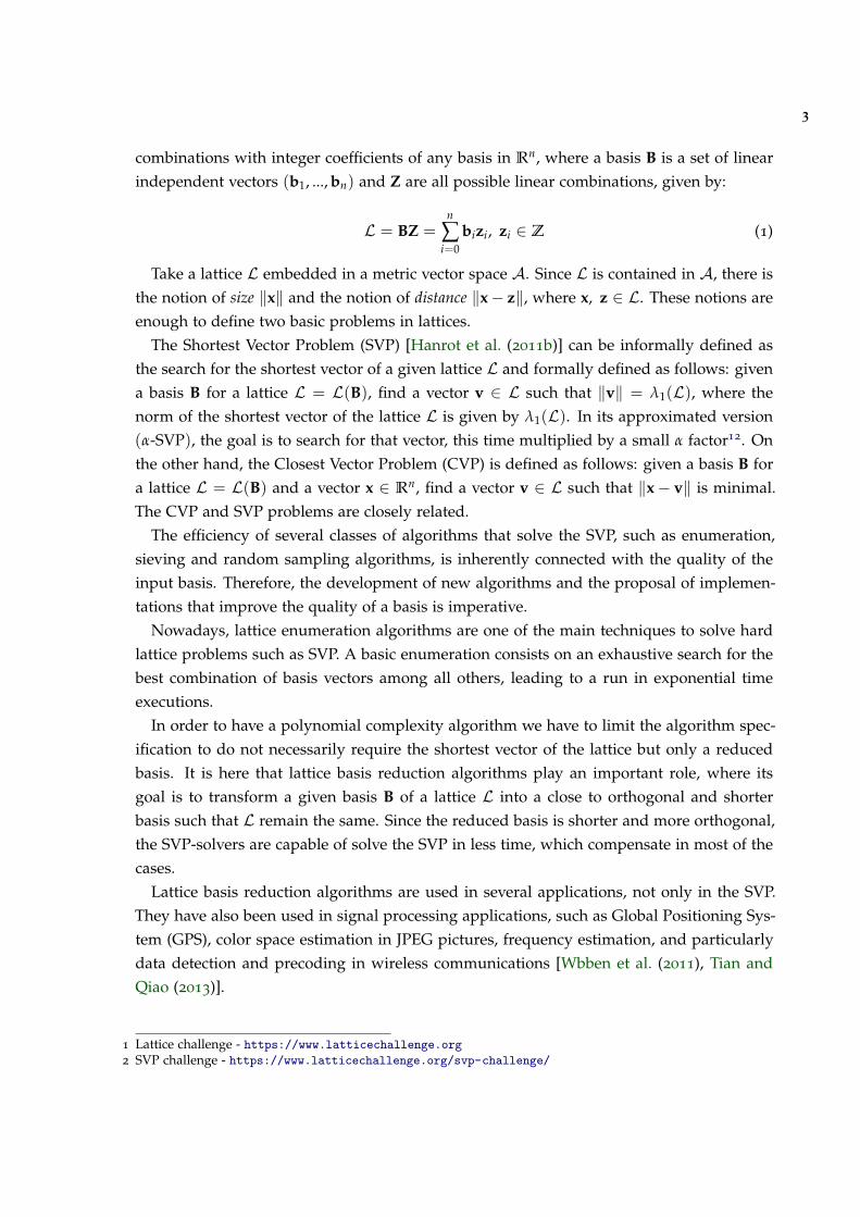
combinations with integer coefficients of any basis in Rn, where a basis B is a set of linearindependent vectors (b1, ..., bn) and Z are all possible linear combinations, given by:

L = BZ =n

∑i=0

bizi, zi ∈ Z (1)

Take a lattice L embedded in a metric vector space A. Since L is contained in A, there isthe notion of size ‖x‖ and the notion of distance ‖x− z‖, where x, z ∈ L. These notions areenough to define two basic problems in lattices.

The Shortest Vector Problem (SVP) [Hanrot et al. (2011b)] can be informally defined asthe search for the shortest vector of a given lattice L and formally defined as follows: givena basis B for a lattice L = L(B), find a vector v ∈ L such that ‖v‖ = λ1(L), where thenorm of the shortest vector of the lattice L is given by λ1(L). In its approximated version(α-SVP), the goal is to search for that vector, this time multiplied by a small α factor12. Onthe other hand, the Closest Vector Problem (CVP) is defined as follows: given a basis B fora lattice L = L(B) and a vector x ∈ Rn, find a vector v ∈ L such that ‖x− v‖ is minimal.The CVP and SVP problems are closely related.

The efficiency of several classes of algorithms that solve the SVP, such as enumeration,sieving and random sampling algorithms, is inherently connected with the quality of theinput basis. Therefore, the development of new algorithms and the proposal of implemen-tations that improve the quality of a basis is imperative.

Nowadays, lattice enumeration algorithms are one of the main techniques to solve hardlattice problems such as SVP. A basic enumeration consists on an exhaustive search for thebest combination of basis vectors among all others, leading to a run in exponential timeexecutions.

In order to have a polynomial complexity algorithm we have to limit the algorithm spec-ification to do not necessarily require the shortest vector of the lattice but only a reducedbasis. It is here that lattice basis reduction algorithms play an important role, where itsgoal is to transform a given basis B of a lattice L into a close to orthogonal and shorterbasis such that L remain the same. Since the reduced basis is shorter and more orthogonal,the SVP-solvers are capable of solve the SVP in less time, which compensate in most of thecases.

Lattice basis reduction algorithms are used in several applications, not only in the SVP.They have also been used in signal processing applications, such as Global Positioning Sys-tem (GPS), color space estimation in JPEG pictures, frequency estimation, and particularlydata detection and precoding in wireless communications [Wbben et al. (2011), Tian andQiao (2013)].

1 Lattice challenge - https://www.latticechallenge.org2 SVP challenge - https://www.latticechallenge.org/svp-challenge/

1.1. Motivation 4

1.1 motivation

Lattice-based cryptography has been a hot topic in the past 10 years, because systems basedon lattices are believed to be secure against quantum computer attacks. These systems arebased on the hardness of the SVP in theory, and of α-SVP in practice. While the SVP hasbeen formulated more than a century ago, the algorithmic study of lattices started only inthe early eighties, and the development of parallel algorithms for the SVP is even morerecent, with developments in the last five years.

Despite the theoretical and practical hardness of the SVP, it is important to keep searchingfor new more efficient implementations or algorithms to prove that a particular problemmay be easier to solve than the expected. The constant scrutiny of these problems is cru-cial to the scientific community, where a particular problem may be considered reliable ornot. Thus, this dissertation focuses on lattice basis reduction algorithms and one of its keyrequirement, MP arithmetic.

1.2 contribution

The work developed during this dissertation targeted performance improvements on latticebasis reduction techniques that lead to scientific contributions. These include:

• Development of an efficient ’Multiple precision Integer Module’ (MpIM)3 with mathe-matical operations, namely addition, increment, subtraction, decrement, multiplica-tion, division, left and right shifts, and several logical operations;

• Development of a ’Lattice Basis Reduction’ (LattBRed)3 module. These include:

– A novel efficient implementation of the Qiao’s Jacobi method;

– Parallel and MP versions of the Qiao’s Jacobi method;

– MP implementations of the LLL and BKZ algorithms.

• A basis quality assessment of the LLL algorithm and Qiao’s Jacobi method for Ajtai-type and Goldstein and Mayer lattice basis.

1.3 roadmap

This dissertation is structured in six chapters. The first chapter introduces the reader thetheme of this dissertation, and briefly explains the relevance of this topic for the scientificcommunity.

3 Module available at https://github.com/heldergoncalves92

1.3. Roadmap 5

The next chapter describes the necessary background to quickly understand the mainsubjects related to lattice basis reduction and describes the computational environmentfor the experimental work. The current approaches for MP and lattice basis reductionalgorithms are presented in this chapter.

Chapter 3 presents the implemented MP operations and compares the module perfor-mance with existing libraries.

Chapter 4 is dedicated to the Qiao’s Jacobi method. It discusses the performance resultsachieved with the sequential and parallel versions of the algorithm and assesses a latticebasis quality of the Qiao’s Jacobi method.

Chapter 5 describes proposed parallel approaches of the LLL and BKZ algorithms andassesses the quality of the output basis of combining the LLL and the BKZ algorithm withthe Qiao’s Jacobi method.

Finally, chapter 6 concludes the dissertation taking into account the obtained results, andleave guidelines for future work that could not be finished or covered.

2

B A C K G R O U N D A N D S E T U P

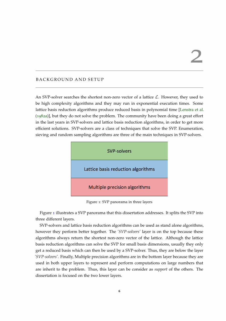
An SVP-solver searches the shortest non-zero vector of a lattice L. However, they used tobe high complexity algorithms and they may run in exponential execution times. Somelattice basis reduction algorithms produce reduced basis in polynomial time [Lenstra et al.(1982a)], but they do not solve the problem. The community have been doing a great effortin the last years in SVP-solvers and lattice basis reduction algorithms, in order to get moreefficient solutions. SVP-solvers are a class of techniques that solve the SVP. Enumeration,sieving and random sampling algorithms are three of the main techniques in SVP-solvers.

Figure 1: SVP panorama in three layers

Figure 1 illustrates a SVP panorama that this dissertation addresses. It splits the SVP intothree different layers.

SVP-solvers and lattice basis reduction algorithms can be used as stand alone algorithms,however they perform better together. The ’SVP-solvers’ layer is on the top because thesealgorithms always return the shortest non-zero vector of the lattice. Although the latticebasis reduction algorithms can solve the SVP for small basis dimensions, usually they onlyget a reduced basis which can then be used by a SVP-solver. Thus, they are below the layer’SVP-solvers’. Finally, Multiple precision algorithms are in the bottom layer because they areused in both upper layers to represent and perform computations on large numbers thatare inherit to the problem. Thus, this layer can be consider as support of the others. Thedissertation is focused on the two lower layers.

6

2.1. Multiple precision 7

2.1 multiple precision

Most current computer architectures support operations between integer scalars with upto 64 bits of precision. However, lattices in cryptography require numbers with a largerprecision to ensure a better security in some applications. MP arithmetic requires the rep-resentation and computation of numbers that do not fit into primitive data types. With thisapproach it is possible to store and perform calculations on numbers whose precision digitsare only limited by the available system memory.

Operations with primitive data types, whose numbers fit into processor registers, areconsiderably faster than the MP arithmetic. While primitive data types are implemented byhardware, MP arithmetic has to be implemented by software.

The MP history starts with a commercial IBM computer in the 50s1. Unlike the currentMP, implemented by software, the IBM 702 implemented a integer arithmetic entirely inhardware on digit strings up to 511 digits. Later in the 60s appear the first widespreadsoftware MP implementation in MACLISP (a dialect of the Lisp programming language).Already in the 80s, the VAX/VMS and VM/CMS were the first operating systems to offerMP functionalities.

This dissertation is focused in MP integer arithmetic, thus the algorithms here presentedare intended to handle large integer numbers.

2.1.1 Current libraries

Current MP libraries are available for many programming languages. Languages such asRuby and Haskell offer built-in support, but its performance decreases. In C and C++, oneof the most used libraries is the GNU Multiple Precision Arithmetic Library (GMP)2.

GMP is a free library for MP arithmetic that was first released in 1991, and it has beenupdated since then. This library aims to have better implementations than any other MPlibrary, mainly because it (i) uses full words to represent a large number, (ii) uses differ-ent algorithms for different operand sizes since the algorithm efficiency depends on theoperand, (iii) is specialized for different processor architectures with highly optimized as-sembly code, and (iv) is continuously updated by the worldwide community.

The Number Theory Library (NTL) is other widely used MP library3. Unlike GMP thatonly implements MP modules, NTL has a strong component in number theory providingdata structures and algorithms (e.g. routines for lattice basis reduction, Gaussian elimina-tion). It makes it way more attractive than GMP when the the research target goes beyondperformance. The NTL author considers it a high-performance library and to increase its

1 Arbitrary precision arithmetic - https://en.wikipedia.org/wiki/Arbitrary-precision_arithmetic2 GMP - https://gmplib.org3 NTL - http://shoup.net/ntl/

2.1. Multiple precision 8

performance when using MP integer arithmetic, the author recommends to compile NTLwith GMP. It also compares the relative performance of NTL against a similar library [Shoup(2016)].

Class Library for Numbers (CLN) is a MP library for efficient computations4. It standsout of the two previously libraries with a rich set of number classes, e.g., rational and com-plex numbers. As most high-performance libraries, it is implemented with C++ whichbrings efficiency, algebraic syntax and type safety. The CLN’s author claims that it isvery efficient in MP integer arithmetic with the use of the Karatsuba algorithm [Karatsubaand Ofman (1962), Karatsuba (1995), Knuth (1997)] and the Fast Fourier Transform (FFT)method [Schonhage and Strassen (1971)]. As most MP libraries, CLN is also dependent ofthe GMP.

The previous MP libraries were consider for further experimental work to this disserta-tion due to its performance and MP number type. However, some well rated libraries werenot considered for further experimental work, namely Multiple-Precision FP computationswith correct Rounding library (MPFR)5 [Fousse et al. (2007)], Modular-positional Floating-point format (MF-format) [Isupov and Knyazkov (2015)], Multiple Precision Integers andRationals library (MPIR)6, Boost7, Multiple Precision Floating-point Interval library (MPFI)8

[Revol and Rouillier (2005)], MPFUN20159, ARPREC10 , GNU Multiple Precision Complex

library (MPC)11, GNU Multi-Precision Rational Interval Arithmetic library (MPRIA)12 andComputer Algebra System (PARI/GP)13. The exclusion of these libraries had several rea-sons: (i) their main functionalities are not relevant in the case study (e.g floating-pointarithmetic, complex numbers, interval arithmetic and others), and (ii) several problemsoccurred when used (e.g. setup or segmentation fault problems and only beta releases).

In addition to these libraries others were also excluded because (i) we could not find rel-evant information about them, (ii) we assumed that their performance was lagging behindsince they were not updated for several years or benchmarks showed that there are more ef-ficient libraries, and (iii) the target programming language is not C/C++. The list includeFast LIbrary for Number Theory (FLINT)14, TTMath Bignum Library (TTMath)15, Arbitrary

4 CLN - http://www.ginac.de/CLN/5 MPFR - http://www.mpfr.org6 MPIR - http://mpir.org7 Boost - http://www.boost.org8 MPFI - http://mpfi.gforge.inria.fr9 MPFUN2015 - http://www.davidhbailey.com/dhbsoftware

10 ARPREC - http://crd-legacy.lbl.gov/~dhbailey/mpdist/11 MPC - http://www.multiprecision.org12 MPRIA - https://www.gnu.org/software/mpria/13 PARI/GP - http://pari.math.u-bordeaux.fr14 FLINT - http://www.flintlib.org15 TTMath - http://www.ttmath.org

2.1. Multiple precision 9

precision library (ApFloat)16, LibTomMath17, CORE Library (CORE)18 [Du et al. (2002)], eX-act Reals in C (XRC)19, Multiple-precision Math (MpMath)20, Software Carry-Save multiple-precision Library (SCSLib) [Defour et al. (2002), Defour and de Dinechin (2003)], Floating-point Arithmetic Library (FpALib)21, Supporting High Precision on Graphics Processors(GARPREC)22, CudA Multiple Precision ARithmetic librarY (CAMPARY)23, General Dec-imal Arithmetic Specification (MPDecimal)24, a Multi-precision Number Theory package(MpNT) [Hritcu et al. (2014), Tiplea et al. (2003)], Piologie25 , BigDigits multiple-precisionarithmetic (BigDigits)26, C for eXtended Scientific Computing (C-XSC) [Hofschuster andKramer (2004)], Multiple precision Integer and Rational Arithmetic C Library (MIRACL)27

[Scott (2016)], My Arbitrary Precision Math library (MAPM)28 [Ring (2001)]and simple andcomplete bignum C library (bigz)29.

2.1.2 Integer Representation

To represent MP numbers, it is necessary to create a structure that supports all computa-tions. The structure must allow efficient computations over the data.

The Residue Number System (RNS) was created by Sun Tsu Suan-Ching in the 4th century.The RNS is based in the Chinese remainder theorem for its operations. It uses a set of smallnumbers that fit in the primitive data types to represent a large MP number. As a largeMP number is composed of a set of smaller numbers, a MP operation can be performed bycompute in parallel and independently each small number.

However, RNS have some limitations, such as the division operation and the compari-son of numbers in order to improve the RNS performance several works have been done[Kaltofen and Hitz (1995), Chren (1990), Isupov and Knyazkov (2015)]. RNS cannot effi-ciently compare two numbers: it has to convert those numbers to other representation toknow, for example, which one is greater. To know more about this representational systemsee [Omondi and Premkumar (2007)].

16 ApFloat - http://www.apfloat.org17 LibTomMath - http://www.libtom.net18 CORE - http://cs.nyu.edu/exact/core_pages/intro.html19 XRC - http://keithbriggs.info/xrc.html20 MpMath - http://mpmath.org/21 FpALib - https://sourceforge.net/projects/precisefloating/22 GARPREC - https://code.google.com/archive/p/gpuprec/23 CAMPARY - http://homepages.laas.fr/mmjoldes/campary/24 MPDecimal - http://www.bytereef.org/mpdecimal/25 Piologie - http://think-automobility.org/geek-stuff/piologie26 BigDigits - http://www.di-mgt.com.au/bigdigits.html27 MIRACL - https://www.miracl.com/28 MAPM - http://www.tc.umn.edu/~ringx004/mapm-main.html29 Bigz - https://sourceforge.net/projects/bigz/

2.1. Multiple precision 10

There are several formats to represent a MP number, but usually it is used an arrayof integer numbers, where we call limb to each position of the array. This dissertationrepresents each limb (usually with 32 or 64 bits) with β. A possible integer representationcontains the following fields:

• Number;

• Size;

• Allocated Size;

• Sign.

The field ’Number’ is an array of integer numbers. Each array position (limb) representsone part of the large number. The large number is always represented in magnitude for aneasier and efficient algorithm implementation without sign verifications. The magnitudeof any number is usually called its absolute value or module. In field ’Number’, one ofthe most critical choices is related to the primitive data type to be used at each position.A susceptible approach is to sel1ect the ’unsigned long’ data type, in C, for each position,which is represented with 64 bits in a 64-bit processor architecture. Libraries such as GMPuse the ’unsigned long’ data type, while other libraries, such as NTL use the ’long’ data type.

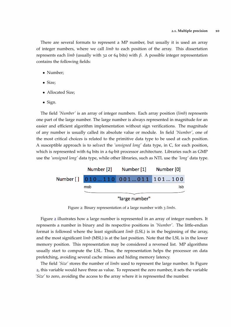
Figure 2: Binary representation of a large number with 3 limbs.

Figure 2 illustrates how a large number is represented in an array of integer numbers. Itrepresents a number in binary and its respective positions in ’Number’. The little-endianformat is followed where the least significant limb (LSL) is in the beginning of the array,and the most significant limb (MSL) is at the last position. Note that the LSL is in the lowermemory position. This representation may be considered a reversed list. MP algorithmsusually start to compute the LSL. Thus, the representation helps the processor on dataprefetching, avoiding several cache misses and hiding memory latency.

The field ’Size’ stores the number of limbs used to represent the large number. In Figure2, this variable would have three as value. To represent the zero number, it sets the variable’Size’ to zero, avoiding the access to the array where it is represented the number.

2.1. Multiple precision 11

The field ’Allocated Size’ contains memory size allocated in bytes for the array ’Number’.This value is always greater than or equal to the variable ’Size’. If there is not enoughmemory allocated, a procedure will do it automatically.

The last field is the ’Sign’. This variable is a boolean and if it is false the number ispositive or zero and if its value is true the number is negative.

There are many ways to represent the number’s sign. A simple format is the representa-tion on the GMP. Contrary to our representation the GMP does not use a field to the signbecause in its representation, the large number’s sign is included in its size variable. A signand magnitude representation is internally used, and the sign bit is used to know the largenumber’s sign. This representation saves some memory, but to determine which is the signor size of the large number, it requires a bit more computation than our representation, i.e.,abs and xor functions and some nested-ifs.

Currently, this approach is implemented in the MP module presented in Chapter 3.

2.1.3 Addition and Subtraction

In MP, the simplest algorithms are the addition and subtraction algorithms, which havea cost of O(n) to a n-limb number. Despite the research of more efficient addition andsubtraction implementations, this approach continues until this day, since new efficientalgorithms have not yet appeared.

The cost of a multiplication is higher than an addition, so fast multiplication algorithms,such as Karatsuba algorithm, are obtained by replacing multiplications by additions.

In MP arithmetic a carry is a digit that is transferred from one column of digits to anothercolumn of more significant digits. The carry is part of the addition algorithm where it startsto compute the LSL and finishes in the MSL.

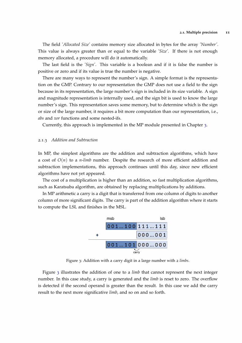
Figure 3: Addition with a carry digit in a large number with 2 limbs.

Figure 3 illustrates the addition of one to a limb that cannot represent the next integernumber. In this case study, a carry is generated and the limb is reset to zero. The overflowis detected if the second operand is greater than the result. In this case we add the carryresult to the next more significative limb, and so on and so forth.

2.1. Multiple precision 12

The MP module implements the addition algorithm (Algorithm 2.1). In line 3, an over-flow may occur, which in turn may generate a carry. Thus, the addition result cannot fit inthe variable s. In this case there are three possibilities to overcome this situation:

• Use a machine instruction that gives the possible carry;

• Compute the module T, t = ai + bi − T. Then, to verify if the carry occurs, do thecomparison t ≤ ai;

• Reserve a bit to check the carry occurrence, taking β ≤ T/2.

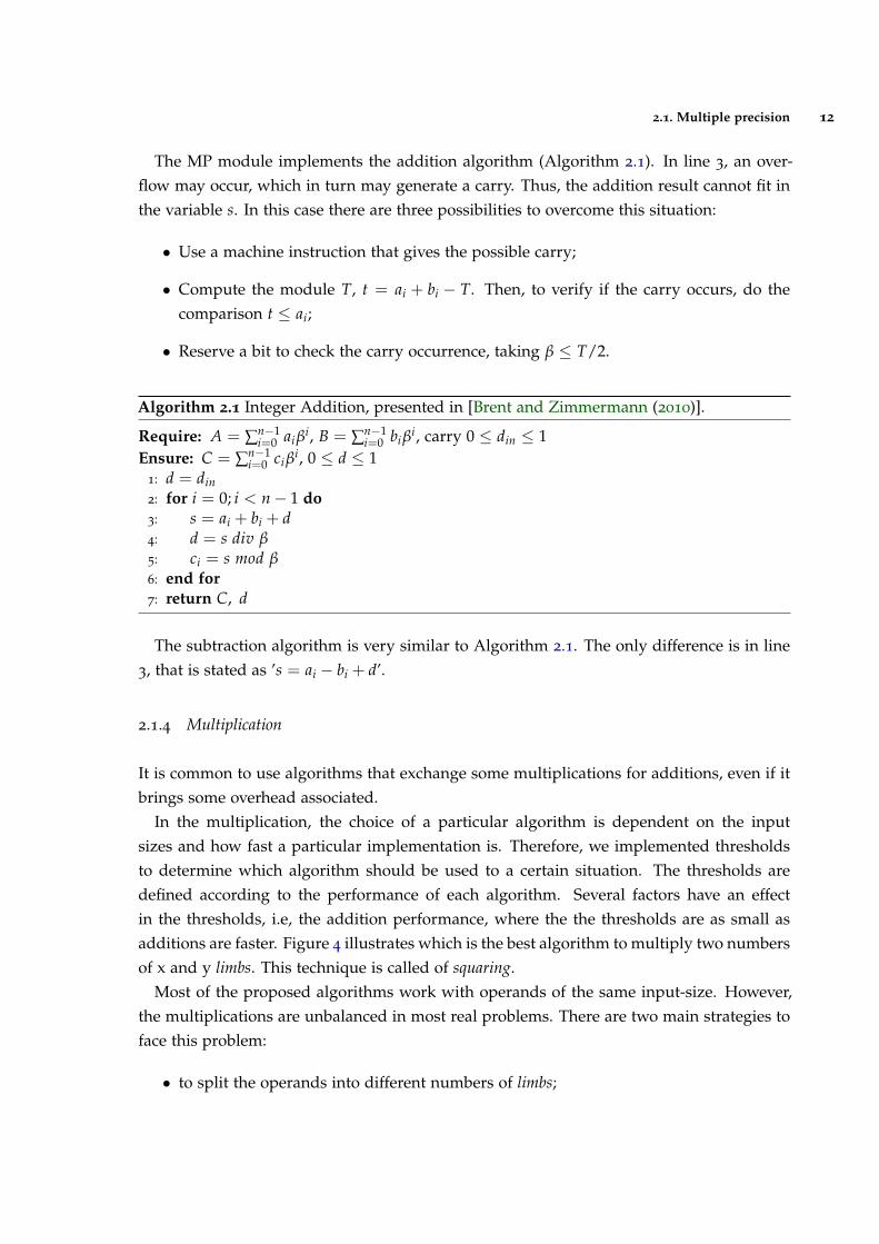
Algorithm 2.1 Integer Addition, presented in [Brent and Zimmermann (2010)].

Require: A = ∑n−1i=0 aiβ

i, B = ∑n−1i=0 biβ

i, carry 0 ≤ din ≤ 1Ensure: C = ∑n−1

i=0 ciβi, 0 ≤ d ≤ 1

1: d = din2: for i = 0; i < n− 1 do3: s = ai + bi + d4: d = s div β5: ci = s mod β6: end for7: return C, d

The subtraction algorithm is very similar to Algorithm 2.1. The only difference is in line3, that is stated as ’s = ai − bi + d’.

2.1.4 Multiplication

It is common to use algorithms that exchange some multiplications for additions, even if itbrings some overhead associated.

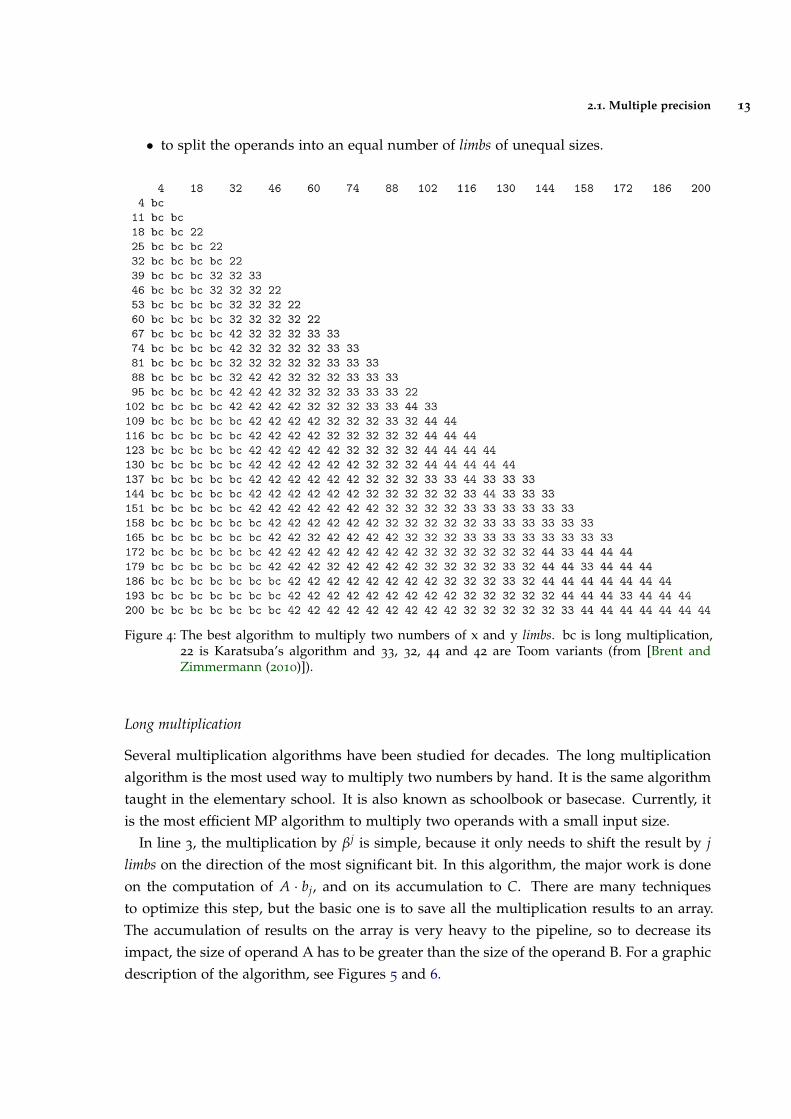
In the multiplication, the choice of a particular algorithm is dependent on the inputsizes and how fast a particular implementation is. Therefore, we implemented thresholdsto determine which algorithm should be used to a certain situation. The thresholds aredefined according to the performance of each algorithm. Several factors have an effectin the thresholds, i.e, the addition performance, where the the thresholds are as small asadditions are faster. Figure 4 illustrates which is the best algorithm to multiply two numbersof x and y limbs. This technique is called of squaring.

Most of the proposed algorithms work with operands of the same input-size. However,the multiplications are unbalanced in most real problems. There are two main strategies toface this problem:

• to split the operands into different numbers of limbs;

2.1. Multiple precision 13

• to split the operands into an equal number of limbs of unequal sizes.

Figure 4: The best algorithm to multiply two numbers of x and y limbs. bc is long multiplication,22 is Karatsuba’s algorithm and 33, 32, 44 and 42 are Toom variants (from [Brent andZimmermann (2010)]).

Long multiplication

Several multiplication algorithms have been studied for decades. The long multiplicationalgorithm is the most used way to multiply two numbers by hand. It is the same algorithmtaught in the elementary school. It is also known as schoolbook or basecase. Currently, itis the most efficient MP algorithm to multiply two operands with a small input size.

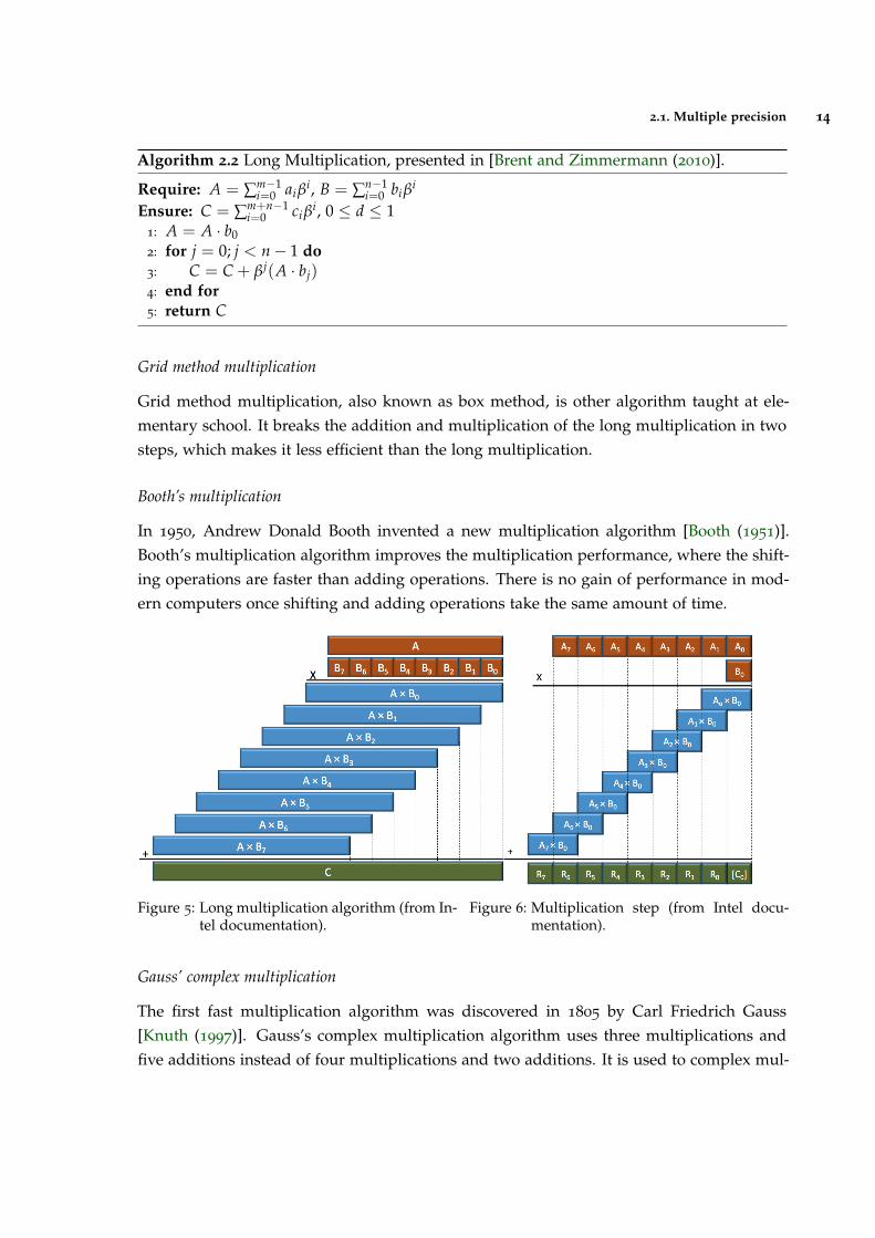
In line 3, the multiplication by βj is simple, because it only needs to shift the result by jlimbs on the direction of the most significant bit. In this algorithm, the major work is doneon the computation of A · bj, and on its accumulation to C. There are many techniquesto optimize this step, but the basic one is to save all the multiplication results to an array.The accumulation of results on the array is very heavy to the pipeline, so to decrease itsimpact, the size of operand A has to be greater than the size of the operand B. For a graphicdescription of the algorithm, see Figures 5 and 6.

2.1. Multiple precision 14

Algorithm 2.2 Long Multiplication, presented in [Brent and Zimmermann (2010)].

Require: A = ∑m−1i=0 aiβ

i, B = ∑n−1i=0 biβ

i

Ensure: C = ∑m+n−1i=0 ciβ

i, 0 ≤ d ≤ 11: A = A · b02: for j = 0; j < n− 1 do3: C = C + βj(A · bj)4: end for5: return C

Grid method multiplication

Grid method multiplication, also known as box method, is other algorithm taught at ele-mentary school. It breaks the addition and multiplication of the long multiplication in twosteps, which makes it less efficient than the long multiplication.

Booth’s multiplication

In 1950, Andrew Donald Booth invented a new multiplication algorithm [Booth (1951)].Booth’s multiplication algorithm improves the multiplication performance, where the shift-ing operations are faster than adding operations. There is no gain of performance in mod-ern computers once shifting and adding operations take the same amount of time.

Figure 5: Long multiplication algorithm (from In-tel documentation).

Figure 6: Multiplication step (from Intel docu-mentation).

Gauss’ complex multiplication

The first fast multiplication algorithm was discovered in 1805 by Carl Friedrich Gauss[Knuth (1997)]. Gauss’s complex multiplication algorithm uses three multiplications andfive additions instead of four multiplications and two additions. It is used to complex mul-

2.1. Multiple precision 15

tiplications, which is not relevant for this dissertation. However, it was the beginning of thefast multiplication algorithms.

Karatsuba

The Divide and Conquer Algorithms (DCA) have a considerable value in MP arithmetic,i.e., Karatsuba and Toom-Cook algorithms [Knuth (1997), Mel (2007), Bodrato (2007)]. DCAare algorithms based on multi-branched recursion. These algorithms work by recursivelybreaking down a problem into two or more sub-problems of the same type, until thesebecome simple enough so no more breakdowns make sense. The solution of the originalproblem is given by the combination of the solution of all the sub-problems generated.

Algorithm 2.3 Karatsuba’s Algorithm, presented in [Brent and Zimmermann (2010)].

Require: A = ∑m−1i=0 aiβ

i, B = ∑n−1i=0 biβ

i

Ensure: C = ∑m+n−1i=0 ciβ

i, 0 ≤ d ≤ 11: if n < n0 then return BaseCaseMultiply(A, B)2: end if3: k = dn/2e4: A0 = A mod βk

5: B0 = B mod βk

6: A1 = A div βk

7: B1 = B div βk

8: sA = sign(A0 − A1)9: sB = sign(B0 − B1)

10: C0 = Karatsuba(A0, B0)11: C1 = Karatsuba(A1, B1)12: C2 = Karatsuba(|A0 − A1|, |B0 − B1|)13: return C = C0 + (C0 + C1 − sAsBC2)βk + C2k

1

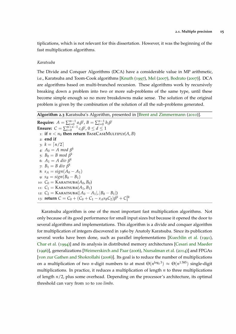
Karatsuba algorithm is one of the most important fast multiplication algorithms. Notonly because of its good performance for small input sizes but because it opened the door toseveral algorithms and implementations. This algorithm is a divide and conquer algorithmfor multiplication of integers discovered in 1960 by Anatoly Karatsuba. Since its publicationseveral works have been done, such as parallel implementations [Kuechlin et al. (1991),Char et al. (1994)] and its analysis in distributed memory architectures [Cesari and Maeder(1996)], generalizations [Weimerskirch and Paar (2006), Nursalman et al. (2014)] and FPGAs[von zur Gathen and Shokrollahi (2006)]. Its goal is to reduce the number of multiplicationson a multiplication of two n-digit numbers to at most Θ(nlog2 3) ≈ Θ(n1.585) single-digitmultiplications. In practice, it reduces a multiplication of length n to three multiplicationsof length n/2, plus some overhead. Depending on the processor’s architecture, its optimalthreshold can vary from 10 to 100 limbs.

2.1. Multiple precision 16

There are many versions of the Karatsuba algorithm, where the addictive and subtractiveversions are the most known. Despite the small difference between them, the subtractiveversion is more attractive since it avoids possible carries. Thus, it is not necessary to havecarry verification step, which makes the subtractive version more efficient.

Algorithm 2.3 illustrates the subtractive Karatsuba version. The different between bothversions is stated as |A0 − A1| and |B0 − B1| instead of A0 + A1 and B0 + B1, at line 12. Inlines 4-7, the operations mod and div are not executed in the implementation. It is only amathematical way to indicate where the large number is split. Here, A0 and B0 have alwaysthe same number of limbs, but A1 and B1 can deal with different sizes.

Toom-Cook k-way

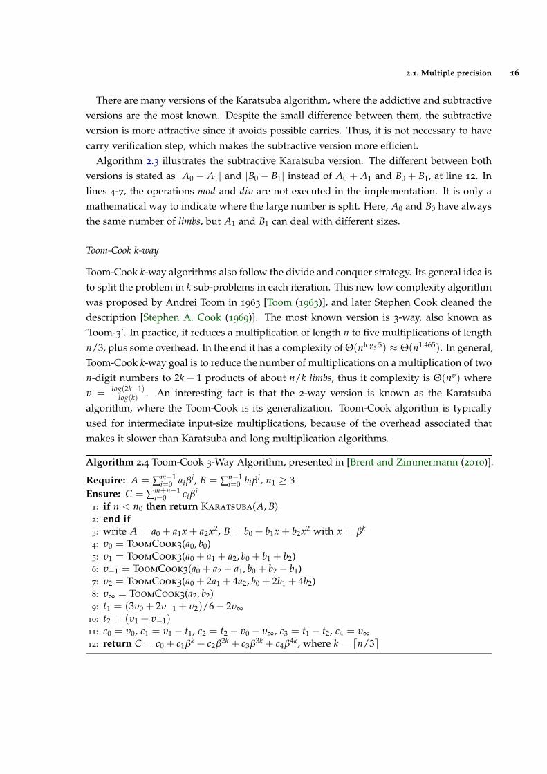
Toom-Cook k-way algorithms also follow the divide and conquer strategy. Its general idea isto split the problem in k sub-problems in each iteration. This new low complexity algorithmwas proposed by Andrei Toom in 1963 [Toom (1963)], and later Stephen Cook cleaned thedescription [Stephen A. Cook (1969)]. The most known version is 3-way, also known as’Toom-3’. In practice, it reduces a multiplication of length n to five multiplications of lengthn/3, plus some overhead. In the end it has a complexity of Θ(nlog3 5) ≈ Θ(n1.465). In general,Toom-Cook k-way goal is to reduce the number of multiplications on a multiplication of twon-digit numbers to 2k− 1 products of about n/k limbs, thus it complexity is Θ(nυ) whereυ = log(2k−1)

log(k) . An interesting fact is that the 2-way version is known as the Karatsubaalgorithm, where the Toom-Cook is its generalization. Toom-Cook algorithm is typicallyused for intermediate input-size multiplications, because of the overhead associated thatmakes it slower than Karatsuba and long multiplication algorithms.

Algorithm 2.4 Toom-Cook 3-Way Algorithm, presented in [Brent and Zimmermann (2010)].

Require: A = ∑m−1i=0 aiβ

i, B = ∑n−1i=0 biβ

i, n1 ≥ 3Ensure: C = ∑m+n−1

i=0 ciβi

1: if n < n0 then return Karatsuba(A, B)2: end if3: write A = a0 + a1x + a2x2, B = b0 + b1x + b2x2 with x = βk

4: υ0 = ToomCook3(a0, b0)5: υ1 = ToomCook3(a0 + a1 + a2, b0 + b1 + b2)6: υ−1 = ToomCook3(a0 + a2 − a1, b0 + b2 − b1)7: υ2 = ToomCook3(a0 + 2a1 + 4a2, b0 + 2b1 + 4b2)8: υ∞ = ToomCook3(a2, b2)9: t1 = (3υ0 + 2υ−1 + υ2)/6− 2υ∞

10: t2 = (υ1 + υ−1)11: c0 = υ0, c1 = υ1 − t1, c2 = t2 − υ0 − υ∞, c3 = t1 − t2, c4 = υ∞12: return C = c0 + c1βk + c2β2k + c3β3k + c4β4k, where k = dn/3e

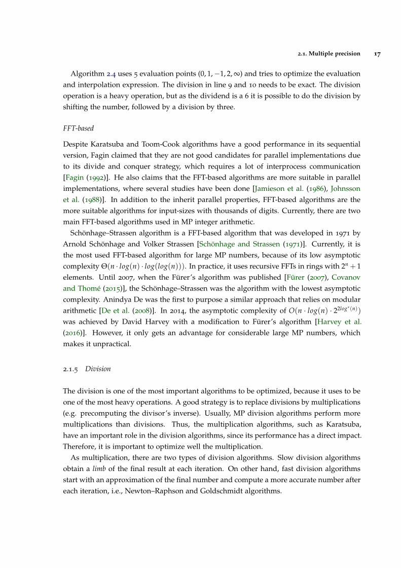
2.1. Multiple precision 17

Algorithm 2.4 uses 5 evaluation points (0, 1,−1, 2, ∞) and tries to optimize the evaluationand interpolation expression. The division in line 9 and 10 needs to be exact. The divisionoperation is a heavy operation, but as the dividend is a 6 it is possible to do the division byshifting the number, followed by a division by three.

FFT-based

Despite Karatsuba and Toom-Cook algorithms have a good performance in its sequentialversion, Fagin claimed that they are not good candidates for parallel implementations dueto its divide and conquer strategy, which requires a lot of interprocess communication[Fagin (1992)]. He also claims that the FFT-based algorithms are more suitable in parallelimplementations, where several studies have been done [Jamieson et al. (1986), Johnssonet al. (1988)]. In addition to the inherit parallel properties, FFT-based algorithms are themore suitable algorithms for input-sizes with thousands of digits. Currently, there are twomain FFT-based algorithms used in MP integer arithmetic.

Schonhage–Strassen algorithm is a FFT-based algorithm that was developed in 1971 byArnold Schonhage and Volker Strassen [Schonhage and Strassen (1971)]. Currently, it isthe most used FFT-based algorithm for large MP numbers, because of its low asymptoticcomplexity Θ(n · log(n) · log(log(n))). In practice, it uses recursive FFTs in rings with 2n + 1elements. Until 2007, when the Furer’s algorithm was published [Furer (2007), Covanovand Thome (2015)], the Schonhage–Strassen was the algorithm with the lowest asymptoticcomplexity. Anindya De was the first to purpose a similar approach that relies on modulararithmetic [De et al. (2008)]. In 2014, the asymptotic complexity of O(n · log(n) · 22log∗(n))

was achieved by David Harvey with a modification to Furer’s algorithm [Harvey et al.(2016)]. However, it only gets an advantage for considerable large MP numbers, whichmakes it unpractical.

2.1.5 Division

The division is one of the most important algorithms to be optimized, because it uses to beone of the most heavy operations. A good strategy is to replace divisions by multiplications(e.g. precomputing the divisor’s inverse). Usually, MP division algorithms perform moremultiplications than divisions. Thus, the multiplication algorithms, such as Karatsuba,have an important role in the division algorithms, since its performance has a direct impact.Therefore, it is important to optimize well the multiplication.

As multiplication, there are two types of division algorithms. Slow division algorithmsobtain a limb of the final result at each iteration. On other hand, fast division algorithmsstart with an approximation of the final number and compute a more accurate number aftereach iteration, i.e., Newton–Raphson and Goldschmidt algorithms.

2.1. Multiple precision 18

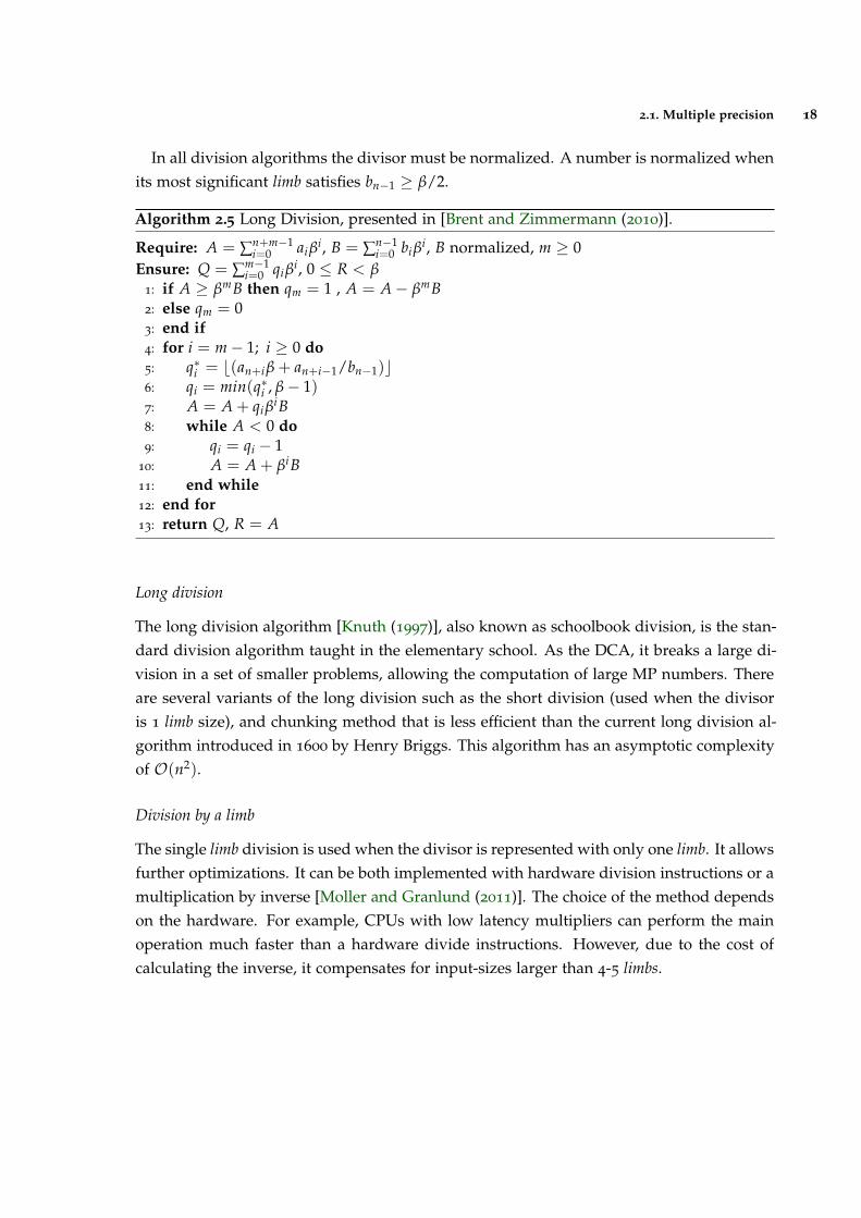
In all division algorithms the divisor must be normalized. A number is normalized whenits most significant limb satisfies bn−1 ≥ β/2.

Algorithm 2.5 Long Division, presented in [Brent and Zimmermann (2010)].

Require: A = ∑n+m−1i=0 aiβ

i, B = ∑n−1i=0 biβ

i, B normalized, m ≥ 0Ensure: Q = ∑m−1

i=0 qiβi, 0 ≤ R < β

1: if A ≥ βmB then qm = 1 , A = A− βmB2: else qm = 03: end if4: for i = m− 1; i ≥ 0 do5: q∗i = b(an+iβ + an+i−1/bn−1)c6: qi = min(q∗i , β− 1)7: A = A + qiβ

iB8: while A < 0 do9: qi = qi − 1

10: A = A + βiB11: end while12: end for13: return Q, R = A

Long division

The long division algorithm [Knuth (1997)], also known as schoolbook division, is the stan-dard division algorithm taught in the elementary school. As the DCA, it breaks a large di-vision in a set of smaller problems, allowing the computation of large MP numbers. Thereare several variants of the long division such as the short division (used when the divisoris 1 limb size), and chunking method that is less efficient than the current long division al-gorithm introduced in 1600 by Henry Briggs. This algorithm has an asymptotic complexityof O(n2).

Division by a limb

The single limb division is used when the divisor is represented with only one limb. It allowsfurther optimizations. It can be both implemented with hardware division instructions or amultiplication by inverse [Moller and Granlund (2011)]. The choice of the method dependson the hardware. For example, CPUs with low latency multipliers can perform the mainoperation much faster than a hardware divide instructions. However, due to the cost ofcalculating the inverse, it compensates for input-sizes larger than 4-5 limbs.

2.1. Multiple precision 19

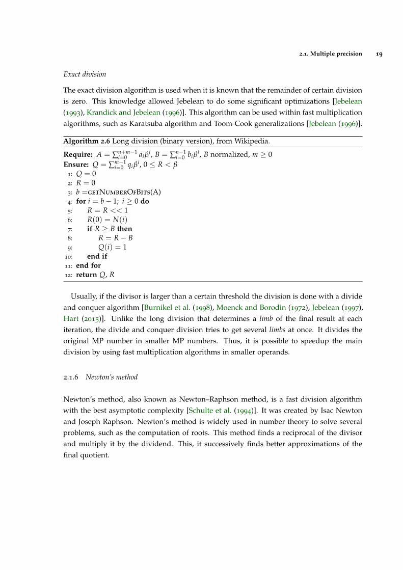
Exact division

The exact division algorithm is used when it is known that the remainder of certain divisionis zero. This knowledge allowed Jebelean to do some significant optimizations [Jebelean(1993), Krandick and Jebelean (1996)]. This algorithm can be used within fast multiplicationalgorithms, such as Karatsuba algorithm and Toom-Cook generalizations [Jebelean (1996)].

Algorithm 2.6 Long division (binary version), from Wikipedia.

Require: A = ∑n+m−1i=0 aiβ

i, B = ∑n−1i=0 biβ

i, B normalized, m ≥ 0Ensure: Q = ∑m−1

i=0 qiβi, 0 ≤ R < β

1: Q = 02: R = 03: b =getNumberOfBits(A)4: for i = b− 1; i ≥ 0 do5: R = R << 16: R(0) = N(i)7: if R ≥ B then8: R = R− B9: Q(i) = 1

10: end if11: end for12: return Q, R

Usually, if the divisor is larger than a certain threshold the division is done with a divideand conquer algorithm [Burnikel et al. (1998), Moenck and Borodin (1972), Jebelean (1997),Hart (2015)]. Unlike the long division that determines a limb of the final result at eachiteration, the divide and conquer division tries to get several limbs at once. It divides theoriginal MP number in smaller MP numbers. Thus, it is possible to speedup the maindivision by using fast multiplication algorithms in smaller operands.

2.1.6 Newton’s method

Newton’s method, also known as Newton–Raphson method, is a fast division algorithmwith the best asymptotic complexity [Schulte et al. (1994)]. It was created by Isac Newtonand Joseph Raphson. Newton’s method is widely used in number theory to solve severalproblems, such as the computation of roots. This method finds a reciprocal of the divisorand multiply it by the dividend. This, it successively finds better approximations of thefinal quotient.

2.1. Multiple precision 20

Barret’s division

Barret’s division is a reduction algorithm created by Paul Barrett in 1986 [Barrett (1987)]to speedup the RSA encryption algorithm on an ’off-the-shelf’ digital signal processingchip. It is designed to replace division by multiplications. Its first version just uses a singlelimb. However, this version is not able to perform MP divisions. Therefore, Barret proposea second version of his algorithm that approximates to the single limb implementation[Menezes et al. (1996)].

2.1.7 Hensel’s division

Classical division algorithms usually cancel the most significant part of the MP number.However, Hensel’s division algorithm cancels the least significant part of the number. Thebig difference of this strategy is that it is not necessary a correction step, since carries go inthe opposite direction of the classical algorithms. There are cases, where only the remainderis desirable. In that cases this algorithm is known as Montgomery reduction [Knezevic et al.(2010)].

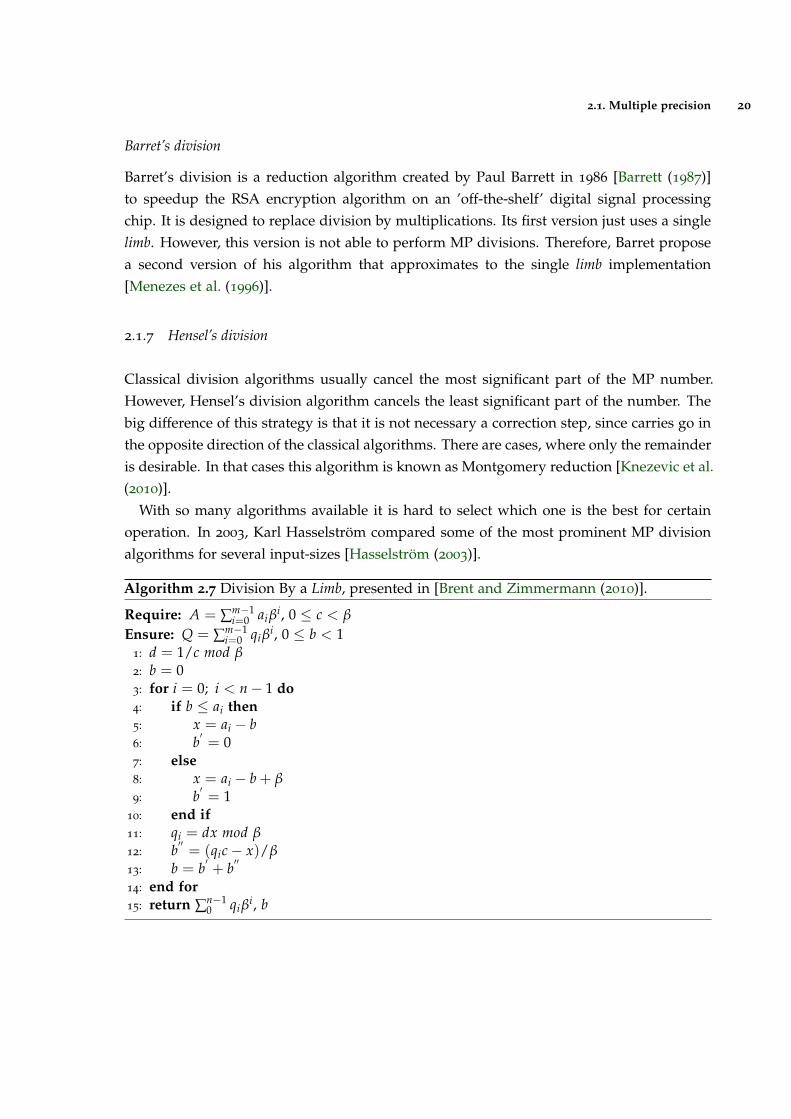
With so many algorithms available it is hard to select which one is the best for certainoperation. In 2003, Karl Hasselstrom compared some of the most prominent MP divisionalgorithms for several input-sizes [Hasselstrom (2003)].

Algorithm 2.7 Division By a Limb, presented in [Brent and Zimmermann (2010)].

Require: A = ∑m−1i=0 aiβ

i, 0 ≤ c < β

Ensure: Q = ∑m−1i=0 qiβ

i, 0 ≤ b < 11: d = 1/c mod β2: b = 03: for i = 0; i < n− 1 do4: if b ≤ ai then5: x = ai − b6: b

′= 0

7: else8: x = ai − b + β9: b

′= 1

10: end if11: qi = dx mod β12: b

′′= (qic− x)/β

13: b = b′+ b

′′

14: end for15: return ∑n−1

0 qiβi, b

2.2. Lattice basis reduction 21

2.2 lattice basis reduction

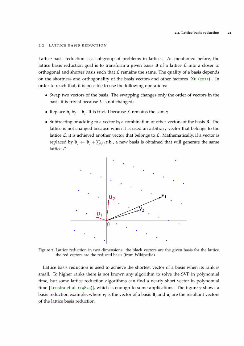
Lattice basis reduction is a subgroup of problems in lattices. As mentioned before, thelattice basis reduction goal is to transform a given basis B of a lattice L into a closer toorthogonal and shorter basis such that L remains the same. The quality of a basis dependson the shortness and orthogonality of the basis vectors and other factores [Xu (2013)]. Inorder to reach that, it is possible to use the following operations:

• Swap two vectors of the basis. The swapping changes only the order of vectors in thebasis it is trivial because L is not changed;

• Replace bj by −bj. It is trivial because L remains the same;

• Subtracting or adding to a vector bj a combination of other vectors of the basis B. Thelattice is not changed because when it is used an arbitrary vector that belongs to thelattice L, it is achieved another vector that belongs to L. Mathematically, if a vector isreplaced by bj ← bj + ∑i 6=j zibi, a new basis is obtained that will generate the samelattice L.

Figure 7: Lattice reduction in two dimensions: the black vectors are the given basis for the lattice,the red vectors are the reduced basis (from Wikipedia).

Lattice basis reduction is used to achieve the shortest vector of a basis when its rank issmall. To higher ranks there is not known any algorithm to solve the SVP in polynomialtime, but some lattice reduction algorithms can find a nearly short vector in polynomialtime [Lenstra et al. (1982a)], which is enough to some applications. The figure 7 shows abasis reduction example, where vi is the vector of a basis B, and ui are the resultant vectorsof the lattice basis reduction.

2.2. Lattice basis reduction 22

Finding a good reduced basis has proved helpful in many fields of computer scienceand mathematics, particularly in cryptology. A good example is the execution time of theSVP-solvers, where they took less time to finish in good quality basis.

2.2.1 Basic Concepts

This section contains some concepts that are important to easily understand about latticesand its inherit problems.

Determinant of a lattice

An interesting feature of a lattice L is its determinant (det L), a relevant numerical invariant.Thus, two different basis with the same lattice L will have the same determinant because itdoes not depend on the choice of a basis B. Geometrically, the determinant is the volumeof the parallelepiped spanned by the basis.

In a full rank basis, where the number of basis vector is equal to the spanned dimen-sion, the determinant of basis B is the volume of the parallelepiped spanned by its vectors.Besides, if the number of vectors is less than the dimension of the underlying space, then

volume is√

det(BTB). In resume for a full rank lattice, we have:

det(L) = det(B) =√

det(BTB) (2)

Gram Matrix

The Gram Matrix of a set of vectors B is a square matrix composed of all possible innerproduct entries (Equation 3). This matrix is symmetric which means that G = GT. It hasimportant applications, such as the computation of linear independences, where a set ofvectors is linearly independent if its determinant is different from zero. It will be widelyused in a lattice reduction algorithm that will be presented ahead.

Gij = 〈Bi, Bj〉 (3)

Gram-Schmidt coefficients

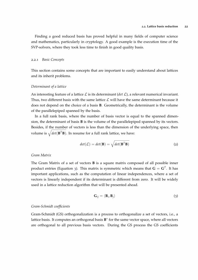
Gram-Schmidt (GS) orthogonalization is a process to orthogonalize a set of vectors, i.e., alattice basis. It computes an orthogonal basis B∗ for the same vector space, where all vectorsare orthogonal to all previous basis vectors. During the GS process the GS coefficients

2.2. Lattice basis reduction 23

and norms are computed. For advantage of some lattice reduction algorithms, the GSorthogonalization is computed iteratively by:

b∗i = bi −j<i

∑j=0

µi,jb∗j , where µi,j =〈bi, b∗j 〉〈b∗j , b∗j 〉

(4)

The GS coefficients (µ) and its norm vectors are widely used in some lattice reductionalgorithms, since it helps to get a more orthogonal basis. Notice that the orthogonal basiscannot belong to the lattice L. Figure 8 illustrates an example of the first two steps of theGS orthogonalization, where ei are normalized vectors.

Figure 8: The first two steps of the Gram–Schmidt orthogonalization (from Wikipedia).

Lattice basis type

Lattice reduction algorithms can have different behaviours depending on the type of inputbasis. Therefore, it is important to study the behaviour of different algorithms in differenttypes of basis.

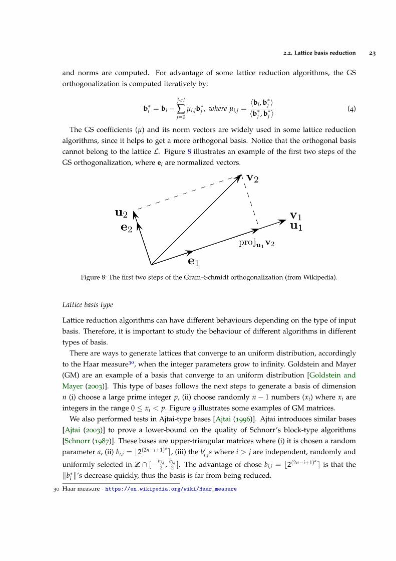
There are ways to generate lattices that converge to an uniform distribution, accordinglyto the Haar measure30, when the integer parameters grow to infinity. Goldstein and Mayer(GM) are an example of a basis that converge to an uniform distribution [Goldstein andMayer (2003)]. This type of bases follows the next steps to generate a basis of dimensionn (i) choose a large prime integer p, (ii) choose randomly n− 1 numbers (xi) where xi areintegers in the range 0 ≤ xi < p. Figure 9 illustrates some examples of GM matrices.

We also performed tests in Ajtai-type bases [Ajtai (1996)]. Ajtai introduces similar bases[Ajtai (2003)] to prove a lower-bound on the quality of Schnorr’s block-type algorithms[Schnorr (1987)]. These bases are upper-triangular matrices where (i) it is chosen a randomparameter a, (ii) bi,i = b2(2n−i+1)ae, (iii) the b′i,js where i > j are independent, randomly and

uniformly selected in Z ∩ [− bj,j2 , bj,j

2 ]. The advantage of chose bi,i = b2(2n−i+1)ae is that the‖b∗i ‖’s decrease quickly, thus the basis is far from being reduced.

30 Haar measure - https://en.wikipedia.org/wiki/Haar_measure

2.2. Lattice basis reduction 24

GM bases have to use MP arithmetic. Besides, Ajtai-type bases can be represented inprimitive data types.

Figure 9: Examples of GM matrices.

2.2.2 Lenstra–Lenstra–Lovasz

The Lenstra–Lenstra–Lovasz (LLL) was the first prominent lattice basis reduction algorithmto be introduced. The LLL is a polynomial time algorithm invented by Arjen Lenstra,Hendrik Lenstra and Laszlo Lovasz in 1982 [Lenstra et al. (1982b)]. Currently, the LLLalgorithm has been successfully implemented, due to the Lovasz condition that controlsswapping operation between basis vectors. Therefore, all of the following works are mainlyfocused on (i) understanding statistical mean running behaviour and average complexity ofthe LLL algorithm [Nguyen and Stehle (2006)] and (ii) improving the efficiency and stabilityof the LLL algorithm [Artur Mariano and Bischof (2016)]. An interesting fact is that manysimulations and theoretical analysis confirm that the LLL algorithm performs much betterin practice than the worst case bound of complexity.

LLL algorithm

The LLL algorithm is split into two main components. The first one aims to make thebasis more orthogonal as possible with the Gram-Schmidt coefficients by computing a size-reduction of the vector bk. It is a size-reduced basis when |µij| ≤ 1

2 , where (1 ≤ j < i ≤ n)in Rn. Usually the basis is size-reduced, but when |µij| > 1

2 it replaces bi with (bi − dµijcbj).The size-reduction component is described in Algorithm 2.8 between lines 4 and 9.

In the second component, it implements the Lovasz swapping condition to make thereduced vectors as short as possible. The Lovasz condition is denoted by:

δ‖b∗i ‖2 ≤ ‖b∗i+1 + µ(i+1)ib∗i ‖2 (5)

where δ = 3/4. A robust swapping condition implies using a larger value for the controlparameter δ in the condition, which can be between 0.95 and 0.999. If the swapping isnecessary, the vectors bi and bi+1 will exchange themselves and then set the current stageof (i + 1) back to i.

2.2. Lattice basis reduction 25

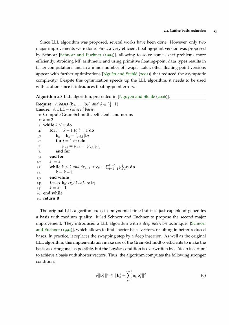
Since LLL algorithm was proposed, several works have been done. However, only twomajor improvements were done. First, a very efficient floating-point version was proposedby Schnorr [Schnorr and Euchner (1994)], allowing to solve some exact problems moreefficiently. Avoiding MP arithmetic and using primitive floating-point data types results infaster computations and in a minor number of swaps. Later, other floating-point versionsappear with further optimizations [Nguen and Stehle (2005)] that reduced the asymptoticcomplexity. Despite this optimization speeds up the LLL algorithm, it needs to be usedwith caution since it introduces floating-point errors.

Algorithm 2.8 LLL algorithm, presented in [Nguyen and Stehle (2006)].

Require: A basis (b1, ..., bn) and δ ∈ ( 14 , 1)

Ensure: A LLL− reduced basis1: Compute Gram-Schmidt coefficients and norms2: k = 23: while k ≤ n do4: for i = k− 1 to i = 1 do5: bk = bk − dµk,icbi6: for j = 1 to i do7: µk,j = µk,j − dµk,icµi,j8: end for9: end for

10: k′ = k11: while k > 2 and δck−1 > ck′ + ∑k′−1

i=k−1 µ2k′,ici do

12: k = k− 113: end while14: Insert bk′ right be f ore bk15: k = k + 116: end while17: return B

The original LLL algorithm runs in polynomial time but it is just capable of generatesa basis with medium quality. It led Schnorr and Euchner to propose the second majorimprovement. They introduced a LLL algorithm with a deep insertion technique. [Schnorrand Euchner (1994)], which allows to find shorter basis vectors, resulting in better reducedbases. In practice, it replaces the swapping step by a deep insertion. As well as the originalLLL algorithm, this implementation make use of the Gram-Schmidt coefficients to make thebasis as orthogonal as possible, but the Lovasz condition is overwritten by a ’deep insertion’to achieve a basis with shorter vectors. Thus, the algorithm computes the following strongercondition:

δ‖b∗i ‖2 ≤ ‖b∗k +k−1

∑j=i

µl jb∗j ‖2 (6)

2.2. Lattice basis reduction 26

where δ = 3/4, until it is true or i < k. If the condition is true the algorithm will insertbk right before bi. Schnorr and Euchner also proposed using a bigger value of δ = 0.99.

At first, the complexity of the LLL algorithm with deep insertions was super polynomial,with examples showing that its practical running time is longer by a few times than theoriginal LLL algorithm, but Gama and Nguyen [Gama and Nguyen (2008)] reported thatthe Schnorr version has super exponential complexity.

2.2.3 Hermite-Korkine-Zolotarev

The Hermite-Korkine-Zolotarev (HKZ) is a lattice-reduction algorithm that achieves re-duced basis with better quality. Its vectors are more orthogonal and shorter than the previ-ous LLL algorithms, but it requires more computation time to converge [Hanrot and Stehle(2008)].

A basis B of a lattice L, is HKZ-reduced if its first vector reaches the minimum of L andif orthogonally projected to b1 the other vectors bi’s are themselves HKZ-reduced.

2.2.4 Block-Korkine-Zolotarev

Schnorr proposed several works during its career. In 1994, he introduces a new lattice ba-sis reduction algorithm [Schnorr and Euchner (1994)]. The Block-Korkine-Zolotarev (BKZ)combines the quality basis output of the HKZ with the good execution times of LLL. Itcombines a lattice basis reduction algorithm with an SVP-solver, the LLL algorithm and anenumeration algorithm respectively. In BKZ, the lattice reduction algorithm and the enu-meration algorithm are dependents on each other, and the enumeration algorithm operatesas a function of the main algorithm.

The BKZ have an extra entry parameter ω that defines the window size. The windowcorresponds to the block of basis vectors where the enumeration algorithm executes. Abigger block size results in a more reduced basis. However, it is necessary some cautionon choosing the window size since the running time increase significantly. It happensbecause the enumeration algorithm is super-exponential, (2O(ω2)). The BKZ with ω = 20is very practical, but when the block size increases to ω ≥ 25, its running time increasessignificantly, which makes any high block size impracticable. This was the Achilles heel ofthe original BKZ, denying the possibility to operate with bigger blocks size.

The BKZ algorithm starts by calling the LLL algorithm to obtain a LLL-reduced basisand then it behaves like a sliding window over the basis, that will call successively anenumeration function, that returns the shortest vector found in the projected basis. Then,if a shorter vector is found, it is added to the current basis and the LLL algorithm is calledagain to remove the generated dependency.

2.2. Lattice basis reduction 27

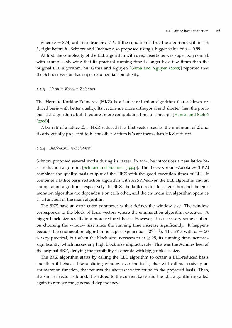
Algorithm 2.9 BKZ algorithm, presented in [Chen and Nguyen (2011)].

Require: A basis (b1, ..., bn), its GramSchmidt orthogonalization, i.e., µ and ci, a block size ω ≥2, and δ ∈ ( 1

4 , 1)Ensure: A BKZ ω− reduced basis

1: z = j = 02: LLL(B, δ)3: while z < n− 1 do4: j = (j mod(n− 1)) + 15: k = min(j + ω− 1, n)6: h = min(k + 1, n)7: v = ENUM(µ, c)8: if v 6= (1, 0, ..., 0) then9: z = 0

10: LLL((b1, ..., ∑ki=j vibi, bj, ..., bh), δ)

11: else12: z = z + 113: LLL((b1, ..., bh), δ)14: end if15: end while16: return B

BKZ 2.0

Lately the BKZ 2.0 was presented by Chen and Nguyen [Chen and Nguyen (2011)], thatmade the first experiments in higher blocks size, ω ≥ 40. The BKZ 2.0 can be consideredan updated BKZ which came with four improvements:

• An early-abort;

• A sound pruning enumeration;

• Preprocessing of local blocks;

• Optimizing the enumeration radius.

The first improvement is simply an early-abort and was based on a theoretical result ofHarrot [Hanrot et al. (2011a)]. This improvement results on the addition of a parameterthat specifies how many iterations should be performed. The improvement delivers anexponential speed up over BKZ over call with higher blocks size.

The other three improvements are related with the enumeration subroutine. The mainmodification consists in the incorporation of the sound pruning technique developed byGama, Nguyen and Regev [Gama et al. (2010)]. The sound pruning uses specific boundingfunctions to discard some branches where the probability of to find a shorter vector is toosmall.

2.2. Lattice basis reduction 28

The cost of the enumeration subroutine is correlated with the quality of the reduced basis.Unfortunately, the BKZ only guarantees an LLL-reduced basis, which can be too expensivewith higher blocks size. Thus, the BKZ 2.0 guarantee a stronger lattice reduction algorithmby preprocessing local blocks.

When the enumeration subroutine starts, the initial radius R used to be initialized asR = ‖b∗j ‖. Unfortunately, this radius could be far from the norm of the shortest vector,what will take more computation than if a nearby radius was defined. However, there is notheoretical proof of which size must be the initial radius. Thus, the radius approximationis based in the Gaussian Heuristic (GH), that provides a good estimate for the norm of theshortest vector of the lattice L. The GH is denoted by:

GH(L) = F(n

2 + 1)

1n × det(L) 1

n (7)

where det(L) is the determinant of the lattice L, and:

F(n) = (n− 1)! (8)

2.2.5 Qiao’s Jacobi method

The Jacobi method proposed by Sanheng Qiao in 2012 is a recent algorithm for lattice basisreduction that claims to reduce a lattice basis with better orthogonality in less time thanLLL algorithm [Qiao (2012)].

The Jacobi method is a very attractive algorithm because it is inherently parallel, due tomatrix computations [Golub and Van Loan (1996)] that are the majority of the algorithm.Thus, there is a great chance to exploit parallel microarchitectures and improve its perfor-mance.

Lagrange’s algorithm computes a reduced basis in a two-dimensional lattice, where S.Qiao found an algorithm that uses this principle, and given a lattice basis A, it gets anunimodular matrix Z of the same size, where AZ forms a reduced basis. The algorithmconsists in applying the two-dimensional Lagrange’s algorithm to all possible pair of vec-tors in original basis A. For a detailed description see the original paper [Qiao (2012)].

The Jacobi method output is said to be Lagrange-reduced (L-reduced). Thus, the basis Ais conspired L-reduced if:

‖ai‖ ≤ ‖aj‖ (9)

|aTi aj| ≤

‖ai‖2

2(10)

where i < j.

2.2. Lattice basis reduction 29

Algorithm 2.10 Qiao’s Jacobi Method, presented in [Qiao (2012)].

Require: An, where n is the lattice dimensionEnsure: Cn = AZ

1: Z = In2: G = ATA3: while !isLagrangeReduced(G) do4: for i = 1 to n− 1 do5: for j = i + 1 to n do6: Z′ =Lagrange(G, i, j)7: Z = ZZ’8: end for9: end for

10: end while11: return C, d

12: function Lagrange(G, i, j)13: Z′ = In14: if Gii < Gjj then15: swap the ith and jth rows of G16: swap the ith and jth column of G17: swap the ith and jth column of Z′

18: end if19: q = bGij/Gjje20: Z = In21: Zii = 0, Zjj = −q, Zij = Zji = 122: G = ZTGZ23: return Z′Z24: end function

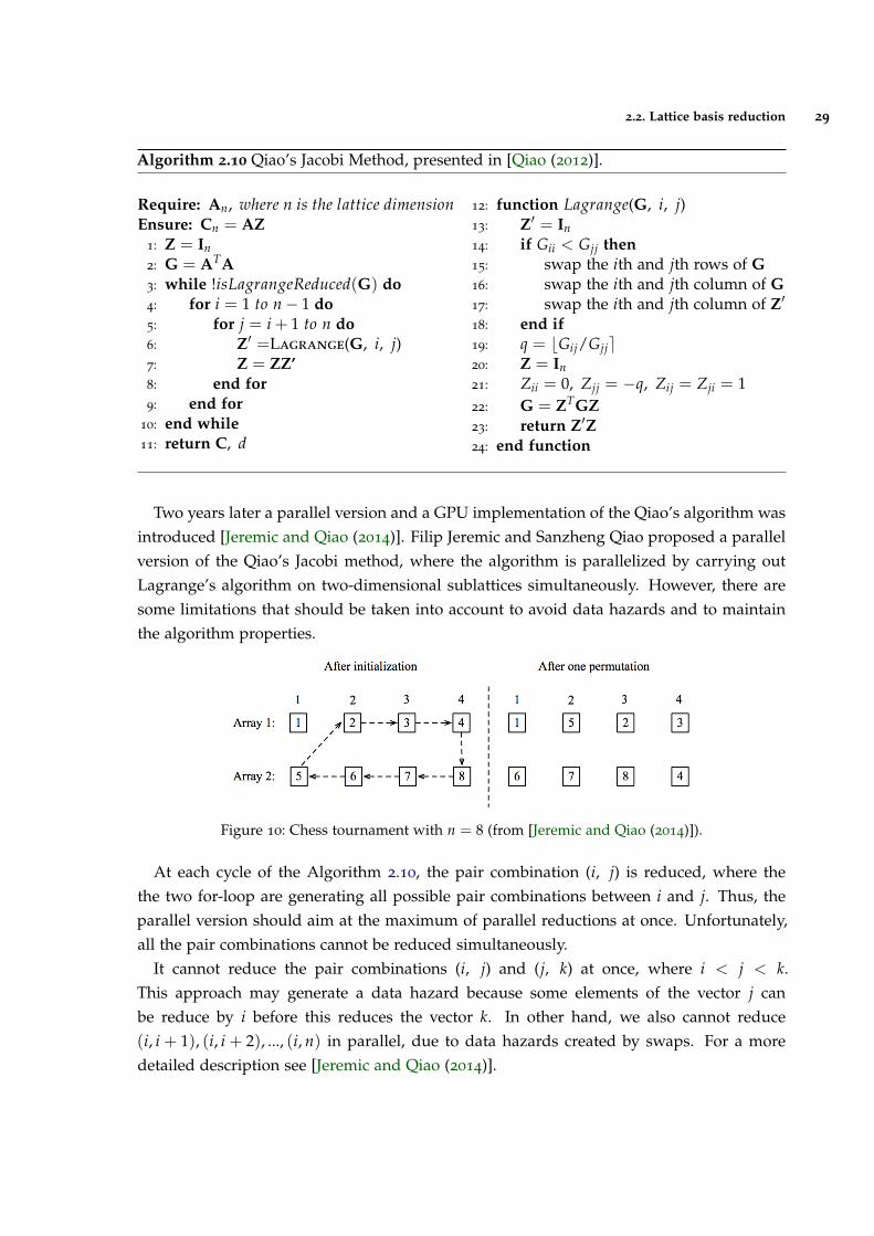
Two years later a parallel version and a GPU implementation of the Qiao’s algorithm wasintroduced [Jeremic and Qiao (2014)]. Filip Jeremic and Sanzheng Qiao proposed a parallelversion of the Qiao’s Jacobi method, where the algorithm is parallelized by carrying outLagrange’s algorithm on two-dimensional sublattices simultaneously. However, there aresome limitations that should be taken into account to avoid data hazards and to maintainthe algorithm properties.

Figure 10: Chess tournament with n = 8 (from [Jeremic and Qiao (2014)]).

At each cycle of the Algorithm 2.10, the pair combination (i, j) is reduced, where thethe two for-loop are generating all possible pair combinations between i and j. Thus, theparallel version should aim at the maximum of parallel reductions at once. Unfortunately,all the pair combinations cannot be reduced simultaneously.

It cannot reduce the pair combinations (i, j) and (j, k) at once, where i < j < k.This approach may generate a data hazard because some elements of the vector j canbe reduce by i before this reduces the vector k. In other hand, we also cannot reduce(i, i + 1), (i, i + 2), ..., (i, n) in parallel, due to data hazards created by swaps. For a moredetailed description see [Jeremic and Qiao (2014)].

2.2. Lattice basis reduction 30

Jeremic suggests the chess tournament ordering [Wang and Qiao (2002)]. It maximizesconcurrency while avoids data hazards and race conditions, and aims to parallelize n/2 paircombinations at once, wherein a column or row only belongs to a pair combination. Thisordering will perform all pair combinations in n− 1 permutations. The first initializationand the first permutation of the chess tournament ordering are illustrated in Figure 10.

The Algorithm 2.10 reduces i against i + 1, i against i + 2, and so on and so forth. Thus,the chess tournament vectors do not follow the same ordering, which may lead to a differentoutput from the original one. Therefore, the algorithm can also take a different number ofsweeps to converge to a solution. One sweep is a double for-loop.

2.2.6 Measuring Basis Quality

The same lattice can be represented by different basis, but it is also crucial to guarantee onlygood basis quality. Besides having a good parallel implementation, it is also important tohave a good basis since these can significantly speedup some applications, namely the SVP.

A lattice basis reduction aims to make the vectors of the reduced basis as short as possibleand as orthogonal as possible. Thus, the basis quality measurements should be relatedwith the lattice reduction goals. It is hard to have a direct evaluation of the output of twodifferent lattice reduction algorithms. To measure the basis quality, we use the followingparameters [Mariano (2016)]:

1. HF of a basis;

2. Sequence of the GS norms;

3. Norm of the last GS vector;

4. Average of the norms of a basis;

5. The product of the norms of a basis;

6. The orthogonal defect of a basis;

7. Execution time of a SVP solver on a lattice.

The basis quality is better for lower values in all mentioned criteria, except for the normof the last GS vector that is best for greater values and the sequence of the GS norms whereit decreases slowly for better basis.

The Hermite Factor (HF) is widely used to measure the quality of different basis. The HFof a basis B of rank n can be defined as:

H(B) =‖b1‖2

vol(L) (11)

2.3. Experimental environment 31

where vol(L) is the volume of a lattice and it is equal to (det(L)) 1n = (det(BTB))

1n . The

volume of lattice is always 1, therefore is directly linked to the square norm of the firstreduced vector. The HF can be interpreted to evaluate the mean and the improvements ofthe length of the shortest reduced vector against the lattice L.

The orthogonal defect, also known as the Hadamard’s inequality, is defined as:

δ(B) =∏n

j=0 ‖bj‖√det(BTB)

(12)

2.3 experimental environment

There are many parallel programming models and a wide variety of implementations,where the purpose of a programming model is to easily adapt a software to multiple plat-forms. The adaptation to the right architecture and technology for a given problem mustbe the first big step of anyone that works in computer science.

Parallel programming is not so easy as it seems, because there is an inherent set ofdifficulties. The biggest disadvantage of parallel programming, but not the hardest toaddress in most cases, is the created computation, overhead, that aims the synchronizationof the running threads. Data races used to be the most common difficulty and sometimesthe most complex to solve. Another common problem is the load balance that can havecertain running patterns, where certain yarns obtain more work, and ultimately have asevere impact on the performance.

To choose the right computing environment it was necessary a thorough study about thetype of algorithms that are presented in this dissertation. Due to several related works, weexplored this case study only on shared memory environments.

2.3.1 Non-Uniform Memory Access

The concept of shared memory allows that several programs access the same memory po-sitions simultaneously. The shared memory allows programs to efficiently communicateor passing data between them. It can avoids redundant copies if data between severalapplications.

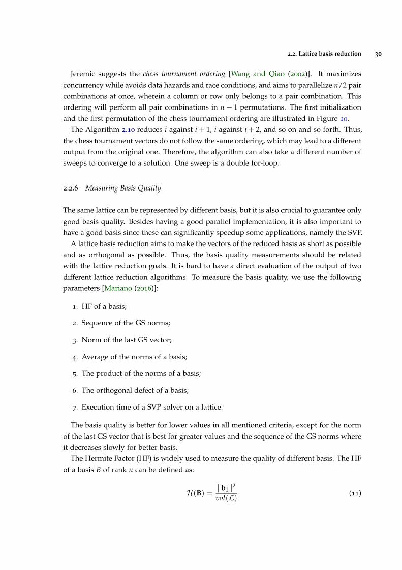
The hardware to a shared memory system is usually referent to a block of memory. Thereare three main types of memory organization to use in a shared memory system:

• Cache-Only Memory Architecture (COMA) - The local memories for the processorsat each node are used as cache instead of actual main memory;

2.3. Experimental environment 32

Figure 11: Shared memory system (from Google Images).

• Non-Uniform Memory Access (NUMA) - Memory access time depends on the mem-ory location relative to a processor;

• Uniform Memory Access (UMA) - All the processors share the physical memory uni-formly, and the access time does not depends of which processor makes the request;

Although three types of memory organization were presented, only NUMA organizationwill be described in greater detail.

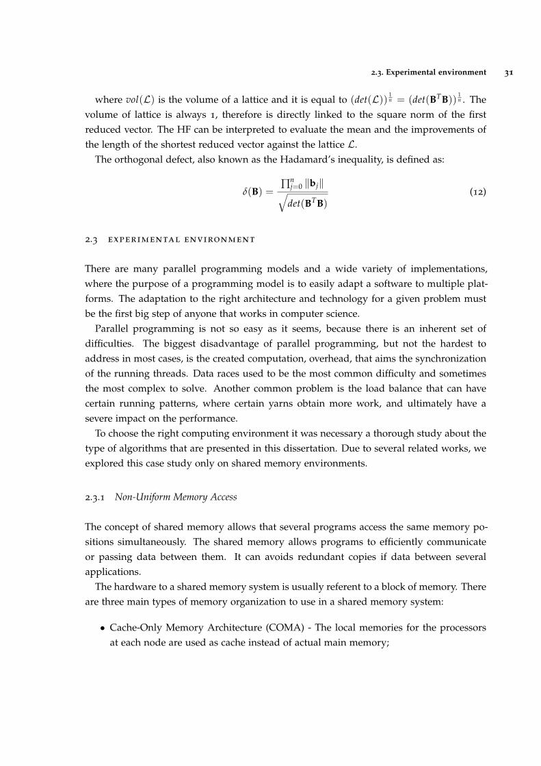
Just one CPU can access to a shared memory system at time, which results in manyrace conditions to the possibility of simultaneous memory accesses. Therefore, in attemptto solve this problem it was created a type of memory organization dedicated to sharedmemory systems called NUMA, that provides separate memory blocks for each CPU, whichallows several memory accesses at each moment.

Figure 12: One possible architecture of a NUMA system (from Advanced Architectures slides).

The NUMA concept gives a global space address to each CPU node, then if a processorneeds to access a memory block in another node, a copy is made to its own local cache.This is the opposite of a COMA memory organization, where the memory block would bemoved instead. Migrate the memory block could bring a better use of memory resourcesand reduce the number of redundant copies, but it can raise the maintenance routines to

2.3. Experimental environment 33

know where is a random memory block at a certain moment. Under a NUMA organizationa certain processor can access its own memory much faster than a memory block in anothernode, where the access time will depend on the distance between both nodes.

2.3.2 Vectorization

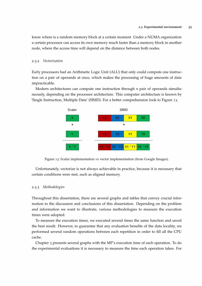
Early processors had an Arithmetic Logic Unit (ALU) that only could compute one instruc-tion on a pair of operands at once, which makes the processing of huge amounts of dataimpracticable.

Modern architectures can compute one instruction through n pair of operands simulta-neously, depending on the processor architecture. This computer architecture is known by’Single Instruction, Multiple Data’ (SIMD). For a better comprehension look to Figure 13.

Figure 13: Scalar implementation vs vector implementation (from Google Images).

Unfortunately, vectorize is not always achievable in practice, because it is necessary thatcertain conditions were met, such as aligned memory.

2.3.3 Methodologies

Throughout this dissertation, there are several graphs and tables that convey crucial infor-mation to the discussion and conclusions of this dissertation. Depending on the problemand information we want to illustrate, various methodologies to measure the executiontimes were adopted.

To measure the execution times, we executed several times the same function and savedthe best result. However, to guarantee that any evaluation benefits of the data locality, weperformed several random operations between each repetition in order to fill all the CPUcache.

Chapter 3 presents several graphs with the MP’s execution time of each operation. To dothe experimental evaluations it is necessary to measure the time each operation takes. For

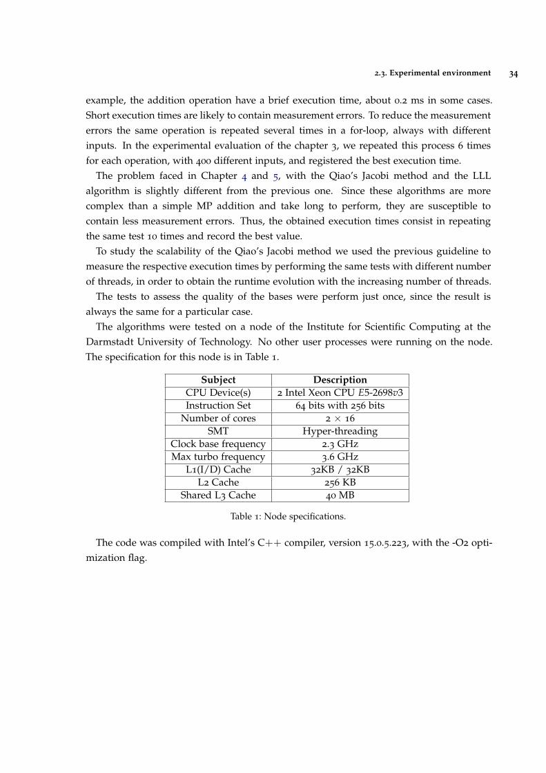
2.3. Experimental environment 34

example, the addition operation have a brief execution time, about 0.2 ms in some cases.Short execution times are likely to contain measurement errors. To reduce the measurementerrors the same operation is repeated several times in a for-loop, always with differentinputs. In the experimental evaluation of the chapter 3, we repeated this process 6 timesfor each operation, with 400 different inputs, and registered the best execution time.

The problem faced in Chapter 4 and 5, with the Qiao’s Jacobi method and the LLLalgorithm is slightly different from the previous one. Since these algorithms are morecomplex than a simple MP addition and take long to perform, they are susceptible tocontain less measurement errors. Thus, the obtained execution times consist in repeatingthe same test 10 times and record the best value.

To study the scalability of the Qiao’s Jacobi method we used the previous guideline tomeasure the respective execution times by performing the same tests with different numberof threads, in order to obtain the runtime evolution with the increasing number of threads.

The tests to assess the quality of the bases were perform just once, since the result isalways the same for a particular case.

The algorithms were tested on a node of the Institute for Scientific Computing at theDarmstadt University of Technology. No other user processes were running on the node.The specification for this node is in Table 1.

Subject DescriptionCPU Device(s) 2 Intel Xeon CPU E5-2698v3Instruction Set 64 bits with 256 bits

Number of cores 2 × 16

SMT Hyper-threadingClock base frequency 2.3 GHzMax turbo frequency 3.6 GHz

L1(I/D) Cache 32KB / 32KBL2 Cache 256 KB

Shared L3 Cache 40 MB

Table 1: Node specifications.

The code was compiled with Intel’s C++ compiler, version 15.0.5.223, with the -O2 opti-mization flag.

3

T H E M U LT I P L E P R E C I S I O N I N T E G E R M O D U L E

This chapter describes the main steps to implement an efficient MP module, referred as the’Multiple precision Integer Module’ (MpIM) in the runtime evaluations of section 3.5. Despitethe several number of MP algorithms presented in the section 2.1, we will take a closer lookat the implemented algorithms.

Every algorithm of the MpIM was subjected to a test validation: to run a given operationwith all possible combinations, with 400 different numbers. This test was repeated fordifferent input-sizes.

3.1 addition and subtraction

In order to get a more efficient implementation, it is always necessary to perform the cal-culations with the absolute number. Thus, the MP addition algorithm implements bothaddiction and subtraction algorithms. Take as example the addition of -8 to 5. Since it isnecessary to guarantee the absolute value, it will perform 8− 5 and then corrects the signof the number.

From the three possibilities reffered in the section 2.1.3 to solve the overflow problem,it is not possible to use the third resolution, since the proposed representation uses the’unsigned long’ as primitive data type. We implemented five versions of the Algorithm 2.1:

1. An implementation with comparisons to detect overflows;

2. An implementation with dedicated Intel intrinsics to MP arithmetic, where the sameinstruction sum the two operands and the carry if there is an overflow on last addition;

3. An assembly implementation;

4. An assembly version that does two additions sequentially avoiding one overflow testper cycle;

5. Vectorized version with AVX 2.0.

35

3.1. Addition and Subtraction 36

Both assembly implementations use an add-with-carry instruction (ADC), and the additionis always done within the CPU registers. Unfortunately, the function inline was not possiblein these versions because of register coherence problems.

We implemented three versions of the subtraction algorithm: (i) an implementation withcomparisons to detect the borrow, (ii) an implementation with dedicated Intel instructionsto MP arithmetic, where the same instruction subtracts the two operands and sum theborrow of the last operation, returning the borrow if it exists in the last subtraction, and (iii)an assembly implementation. The borrow is the subtraction special case for the overflow inthe addition.

The second implementation of the addition algorithm uses the ’ addcarry u64’ Intel intrin-sic, and the subtraction algorithm uses the ’ subborrow u64’ Intel intrinsic.

3.1.1 Addition Vectorization

The result of the limb i rely on the result of the limb i− 1 due to overflow problems. Thereis a chance to vectorize this algorithm, but it could take some overhead.

It is not possible to vectorize the Algorithm 2.1 and keep the cost of O(n) to a n-limbnumber. With AVX 2.0, it is possible to get a good theoretical speedup (four times faster), byvectorizing four additions. If there are no carries on the comparison test, the best scenariois achieved. However, the worst scenario gets more computation and could be slower thanthe basic algorithm. It happens if a carry is identified in every comparison tests.

AVX and AVX 2.0 do not support comparisons of unsigned numbers, which makes itimpossible to implement this strategy. The best chance to implement it, it is with Broadwellmicroarchitecture that supports AVX-512.

The implemented version does four additions at once. Then it compares the result to theoperand, limb by limb and adds the carry on next limb more significant. The intrinsics usedwere:

• mm256 load si256;

• mm256 store si256;

• mm256 add epi64.

3.1.2 Increment and Decrement

The increment/decrement algorithm is similar to the addition/subtraction algorithm. Theincrement and decrement operators are unary operators that add or subtract one from theiroperand, respectively. The main difference is that the algorithm only does one addition or

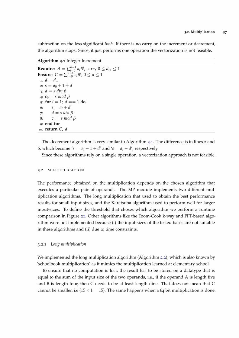
3.2. Multiplication 37

subtraction on the less significant limb. If there is no carry on the increment or decrement,the algorithm stops. Since, it just performs one operation the vectorization is not feasible.

Algorithm 3.1 Integer Increment

Require: A = ∑n−1i=0 aiβ

i, carry 0 ≤ din ≤ 1Ensure: C = ∑n−1

i=0 ciβi, 0 ≤ d ≤ 1

1: d = din2: s = a0 + 1 + d3: d = s div β4: c0 = s mod β5: for i = 1; d == 1 do6: s = ai + d7: d = s div β8: ci = s mod β9: end for

10: return C, d

The decrement algorithm is very similar to Algorithm 3.1. The difference is in lines 2 and6, which become ‘s = a0 − 1 + d’ and ‘s = ai − d’, respectively.

Since these algorithms rely on a single operation, a vectorization approach is not feasible.

3.2 multiplication

The performance obtained on the multiplication depends on the chosen algorithm thatexecutes a particular pair of operands. The MP module implements two different mul-tiplication algorithms. The long multiplication that used to obtain the best performanceresults for small input-sizes, and the Karatsuba algorithm used to perform well for largerinput-sizes. To define the threshold that choses which algorithm we perform a runtimecomparison in Figure 21. Other algorithms like the Toom-Cook k-way and FFT-based algo-rithm were not implemented because (i) the input-sizes of the tested bases are not suitablein these algorithms and (ii) due to time constraints.

3.2.1 Long multiplication

We implemented the long multiplication algorithm (Algorithm 2.2), which is also known by’schoolbook multiplication’ as it mimics the multiplication learned at elementary school.

To ensure that no computation is lost, the result has to be stored on a datatype that isequal to the sum of the input size of the two operands, i.e., if the operand A is length fiveand B is length four, then C needs to be at least length nine. That does not mean that Ccannot be smaller, i.e (15× 1 = 15). The same happens when a 64 bit multiplication is done.

3.2. Multiplication 38

Thus, the implementation uses the ’unsigned int128’ data type, in C++, that has 128 bitsof precision. This data type is a C++ extension. In reality, it is a struct of two ’unsignedlong’, where simple operations like addition and multiplication are optimized at compilerlevel.

We implement the long multiplication algorithm in two ways: (i) an implementation thatuses the ’unsigned int128’ data type to save the multiplication result and then accumulatethe two halves of the result, and (ii) an implementation with a late Intel instruction, availableon the Haswell microarchitecture and folling ones, which aims to increase the performanceof MP multiplications. The Intel intrinsic is the ’ mulx u64’. This instruction is an extensionof the existing multiplication instruction but has two main advantages:

• Greater flexibility in register usage. The default multiply instruction have the destina-tion registers implicity defined. With MULX, the destination registers may be distinctfrom the source operands, so that the source operands are not overwritten;

• Since no flags are modified, MULX instructions can be mixed with add-carry instruc-tions without corrupting the carry chain;

To optimize even further the long multiplication, it is recommend to allocate a block ofmemory to store the multiplication result. It allows the loop-unroll of several multiplica-tions in order to maximize multiplication throughput. Unfortunately, this technique wasnot implemented due to time constraints.

There are two more new instructions to support large integer arithmetic. The ADCX andthe ADOX instructions are extension of the existing ADC but these two instructions aredesigned to support two different carry-chains concurrently. Since these instructions areavailable from Broadwell microarchitecture, the required hardware is not available.

Currently, it is impossible to vectorize this algorithm with the current unsigned long datatype because there are any vector instructions that multiply two unsigned 64 bit lengthnumbers and return an unsigned 128 bit length limb.

3.2.2 Karatsuba

A good implementation of the Karatsuba algorithm must rely on a good use of allocatedmemory. Thus, a good improvement is to avoid allocating memory for the intermediateresults C0, C1, C2, |A0 − A1| and |B0 − B1|, where a possible solution is to allocate a largeamount of memory on the first call of the algorithm. Our implementation computes howmuch memory will be necessary in the beginning and allocates memory just once.

Algorithm 2.3 represents a multiplication where both operands have the same input-size.However, it does not work in most real cases where the operands have different input-sizes.To handle with this problem the line 1 is a bit different. It handles a second condition that

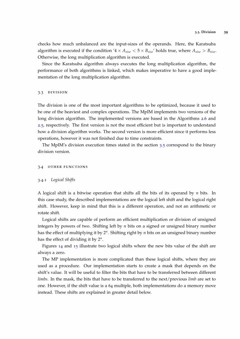
3.3. Division 39

checks how much unbalanced are the input-sizes of the operands. Here, the Karatsubaalgorithm is executed if the condition ’4× Asize < 5× Bsize’ holds true, where Asize > Bsize.Otherwise, the long multiplication algorithm is executed.

Since the Karatsuba algorithm always executes the long multiplication algorithm, theperformance of both algorithms is linked, which makes imperative to have a good imple-mentation of the long multiplication algorithm.

3.3 division

The division is one of the most important algorithms to be optimized, because it used tobe one of the heaviest and complex operations. The MpIM implements two versions of thelong division algorithm. The implemented versions are based in the Algorithms 2.6 and2.5, respectively. The first version is not the most efficient but is important to understandhow a division algorithm works. The second version is more efficient since it performs lessoperations, however it was not finished due to time constraints.

The MpIM’s division execution times stated in the section 3.5 correspond to the binarydivision version.

3.4 other functions

3.4.1 Logical Shifts

A logical shift is a bitwise operation that shifts all the bits of its operand by n bits. Inthis case study, the described implementations are the logical left shift and the logical rightshift. However, keep in mind that this is a different operation, and not an arithmetic orrotate shift.

Logical shifts are capable of perform an efficient multiplication or division of unsignedintegers by powers of two. Shifting left by n bits on a signed or unsigned binary numberhas the effect of multiplying it by 2n. Shifting right by n bits on an unsigned binary numberhas the effect of dividing it by 2n.

Figures 14 and 15 illustrate two logical shifts where the new bits value of the shift arealways a zero.

The MP implementation is more complicated than these logical shifts, where they areused as a procedure. Our implementation starts to create a mask that depends on theshift’s value. It will be useful to filter the bits that have to be transferred between differentlimbs. In the mask, the bits that have to be transferred to the next/previous limb are set toone. However, if the shift value is a 64 multiple, both implementations do a memory moveinstead. These shifts are explained in greater detail below.

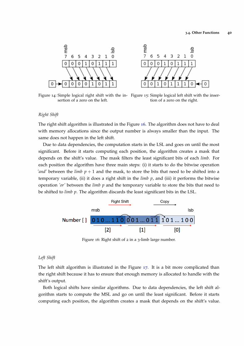
3.4. Other Functions 40

Figure 14: Simple logical right shift with the in-sertion of a zero on the left.

Figure 15: Simple logical left shift with the inser-tion of a zero on the right.

Right Shift

The right shift algorithm is illustrated in the Figure 16. The algorithm does not have to dealwith memory allocations since the output number is always smaller than the input. Thesame does not happen in the left shift.

Due to data dependencies, the computation starts in the LSL and goes on until the mostsignificant. Before it starts computing each position, the algorithm creates a mask thatdepends on the shift’s value. The mask filters the least significant bits of each limb. Foreach position the algorithm have three main steps: (i) it starts to do the bitwise operation’and’ between the limb p + 1 and the mask, to store the bits that need to be shifted into atemporary variable, (ii) it does a right shift in the limb p, and (iii) it performs the bitwiseoperation ’or’ between the limb p and the temporary variable to store the bits that need tobe shifted to limb p. The algorithm discards the least significant bits in the LSL.

Figure 16: Right shift of 2 in a 3-limb large number.

Left Shift

The left shift algorithm is illustrated in the Figure 17. It is a bit more complicated thanthe right shift because it has to ensure that enough memory is allocated to handle with theshift’s output.

Both logical shifts have similar algorithms. Due to data dependencies, the left shift al-gorithm starts to compute the MSL and go on until the least significant. Before it startscomputing each position, the algorithm creates a mask that depends on the shift’s value.

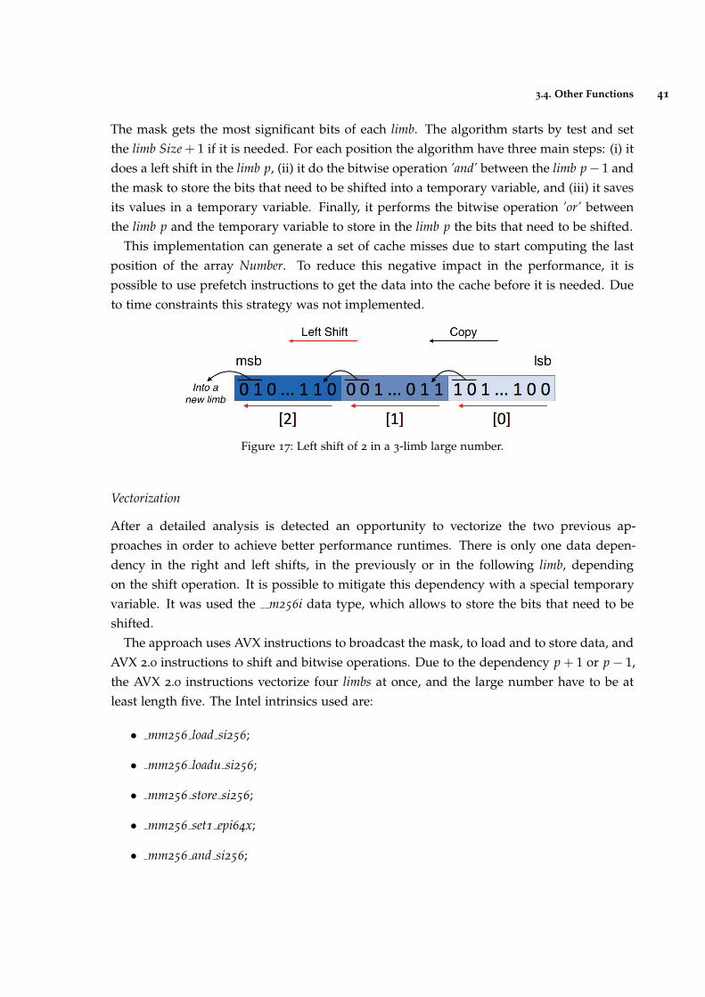
3.4. Other Functions 41

The mask gets the most significant bits of each limb. The algorithm starts by test and setthe limb Size + 1 if it is needed. For each position the algorithm have three main steps: (i) itdoes a left shift in the limb p, (ii) it do the bitwise operation ’and’ between the limb p− 1 andthe mask to store the bits that need to be shifted into a temporary variable, and (iii) it savesits values in a temporary variable. Finally, it performs the bitwise operation ’or’ betweenthe limb p and the temporary variable to store in the limb p the bits that need to be shifted.

This implementation can generate a set of cache misses due to start computing the lastposition of the array Number. To reduce this negative impact in the performance, it ispossible to use prefetch instructions to get the data into the cache before it is needed. Dueto time constraints this strategy was not implemented.

Figure 17: Left shift of 2 in a 3-limb large number.

Vectorization

After a detailed analysis is detected an opportunity to vectorize the two previous ap-proaches in order to achieve better performance runtimes. There is only one data depen-dency in the right and left shifts, in the previously or in the following limb, dependingon the shift operation. It is possible to mitigate this dependency with a special temporaryvariable. It was used the m256i data type, which allows to store the bits that need to beshifted.

The approach uses AVX instructions to broadcast the mask, to load and to store data, andAVX 2.0 instructions to shift and bitwise operations. Due to the dependency p + 1 or p− 1,the AVX 2.0 instructions vectorize four limbs at once, and the large number have to be atleast length five. The Intel intrinsics used are:

• mm256 load si256;

• mm256 loadu si256;

• mm256 store si256;

• mm256 set1 epi64x;

• mm256 and si256;

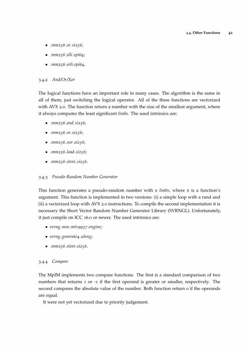
3.4. Other Functions 42

• mm256 or si256;

• mm256 slli epi64;

• mm256 srli epi64.

3.4.2 And/Or/Xor

The logical functions have an important role in many cases. The algorithm is the same inall of them, just switching the logical operator. All of the three functions are vectorizedwith AVX 2.0. The function return a number with the size of the smallest argument, whereit always computes the least significant limbs. The used intrinsics are:

• mm256 and si256;

• mm256 or si256;

• mm256 xor si256;

• mm256 load si256;

• mm256 store si256.

3.4.3 Pseudo-Random Number Generator

This function generates a pseudo-random number with n limbs, where n is a function’sargument. This function is implemented in two versions: (i) a simple loop with a rand and(ii) a vectorized loop with AVX 2.0 instructions. To compile the second implementation it isnecessary the Short Vector Random Number Generator Library (SVRNGL). Unfortunately,it just compile on ICC 16.0 or newer. The used intrinsics are:

• svrng new mt19937 engine;

• svrng generate4 ulong;

• mm256 store si256.

3.4.4 Compare

The MpIM implements two compare functions. The first is a standard comparison of twonumbers that returns 1 or -1 if the first operand is greater or smaller, respectively. Thesecond compares the absolute value of the number. Both function return 0 if the operandsare equal.

It were not yet vectorized due to priority judgement.

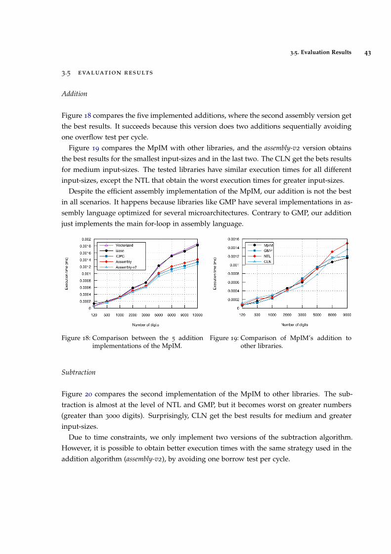
3.5. Evaluation Results 43

3.5 evaluation results

Addition

Figure 18 compares the five implemented additions, where the second assembly version getthe best results. It succeeds because this version does two additions sequentially avoidingone overflow test per cycle.

Figure 19 compares the MpIM with other libraries, and the assembly-v2 version obtainsthe best results for the smallest input-sizes and in the last two. The CLN get the bets resultsfor medium input-sizes. The tested libraries have similar execution times for all differentinput-sizes, except the NTL that obtain the worst execution times for greater input-sizes.

Despite the efficient assembly implementation of the MpIM, our addition is not the bestin all scenarios. It happens because libraries like GMP have several implementations in as-sembly language optimized for several microarchitectures. Contrary to GMP, our additionjust implements the main for-loop in assembly language.

Figure 18: Comparison between the 5 additionimplementations of the MpIM.

Figure 19: Comparison of MpIM’s addition toother libraries.

Subtraction

Figure 20 compares the second implementation of the MpIM to other libraries. The sub-traction is almost at the level of NTL and GMP, but it becomes worst on greater numbers(greater than 3000 digits). Surprisingly, CLN get the best results for medium and greaterinput-sizes.

Due to time constraints, we only implement two versions of the subtraction algorithm.However, it is possible to obtain better execution times with the same strategy used in theaddition algorithm (assembly-v2), by avoiding one borrow test per cycle.

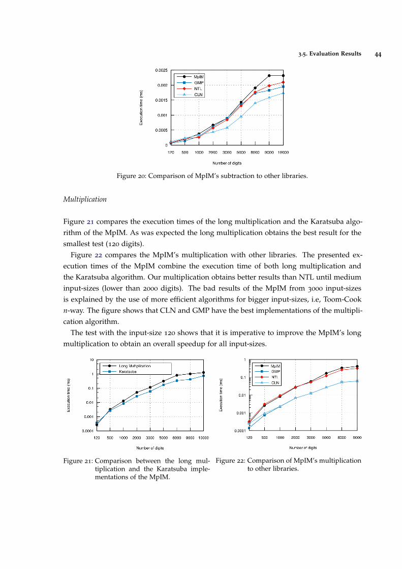
3.5. Evaluation Results 44

Figure 20: Comparison of MpIM’s subtraction to other libraries.

Multiplication

Figure 21 compares the execution times of the long multiplication and the Karatsuba algo-rithm of the MpIM. As was expected the long multiplication obtains the best result for thesmallest test (120 digits).

Figure 22 compares the MpIM’s multiplication with other libraries. The presented ex-ecution times of the MpIM combine the execution time of both long multiplication andthe Karatsuba algorithm. Our multiplication obtains better results than NTL until mediuminput-sizes (lower than 2000 digits). The bad results of the MpIM from 3000 input-sizesis explained by the use of more efficient algorithms for bigger input-sizes, i.e, Toom-Cookn-way. The figure shows that CLN and GMP have the best implementations of the multipli-cation algorithm.

The test with the input-size 120 shows that it is imperative to improve the MpIM’s longmultiplication to obtain an overall speedup for all input-sizes.

Figure 21: Comparison between the long mul-tiplication and the Karatsuba imple-mentations of the MpIM.

Figure 22: Comparison of MpIM’s multiplicationto other libraries.

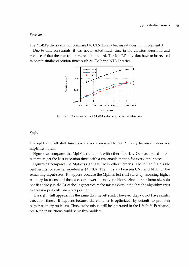
3.5. Evaluation Results 45

Division

The MpIM’s division is not compared to CLN library because it does not implement it.Due to time constraints, it was not invested much time in the division algorithm and

because of that the best results were not obtained. The MpIM’s division have to be revisedto obtain similar execution times such as GMP and NTL libraries.

Figure 23: Comparison of MpIM’s division to other libraries.

Shifts

The right and left shift functions are not compared to GMP library because it does notimplement them.

Figures 24 compares the MpIM’s right shift with other libraries. Our vectorized imple-mentation get the best execution times with a reasonable margin for every input-sizes.

Figures 25 compares the MpIM’s right shift with other libraries. The left shift stats thebest results for smaller input-sizes (≤ 500). Then, it stats between CNL and NTL for theremaining input-sizes. It happens because the MpIm’s left shift starts by accessing highermemory locations and then accesses lower memory positions. Since larger input-sizes donot fit entirely in the L1 cache, it generates cache misses every time that the algorithm triesto access a particular memory position.

The right shift approach is the same that the left shift. However, they do not have similarexecution times. It happens because the compiler is optimized, by default, to pre-fetchhigher memory positions. Thus, cache misses will be generated in the left shift. Perchance,pre-fetch instructions could solve this problem.

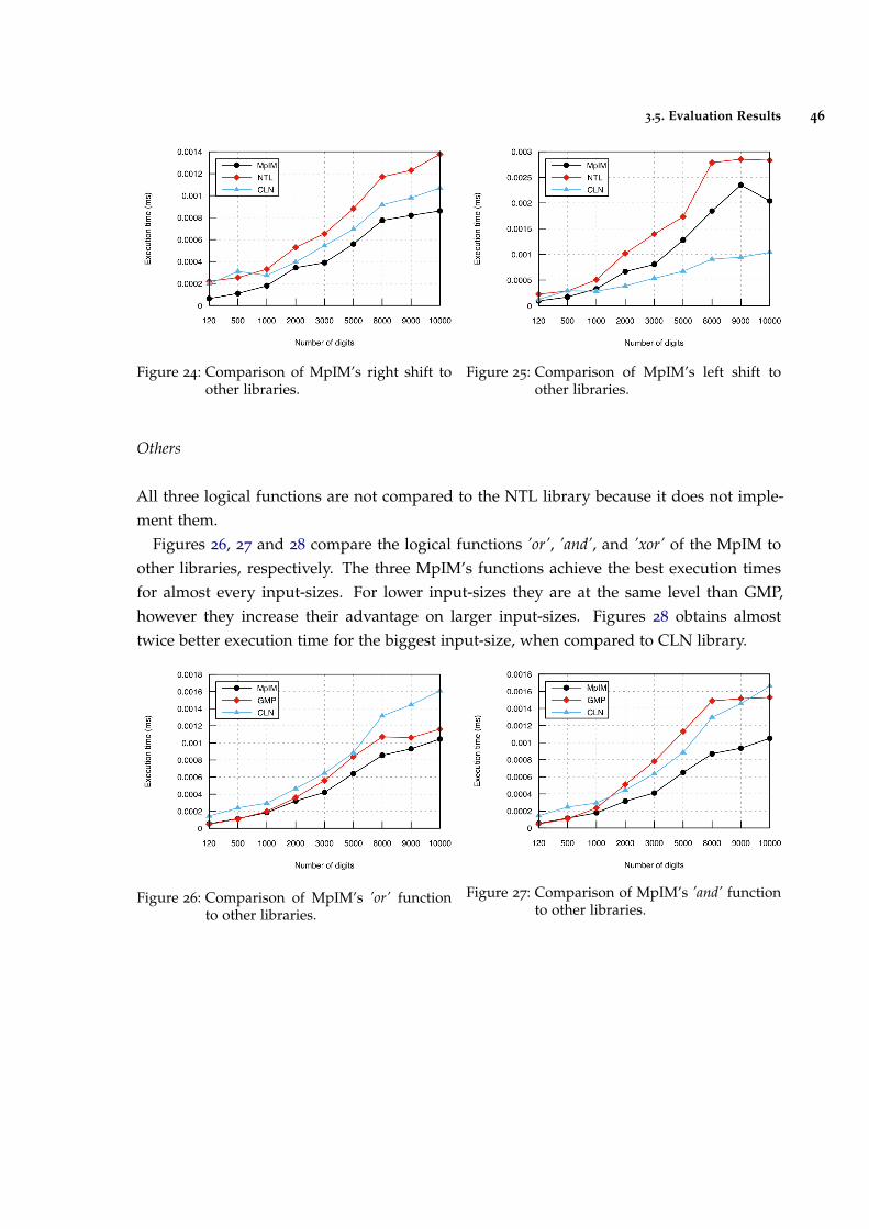
3.5. Evaluation Results 46

Figure 24: Comparison of MpIM’s right shift toother libraries.

Figure 25: Comparison of MpIM’s left shift toother libraries.

Others

All three logical functions are not compared to the NTL library because it does not imple-ment them.

Figures 26, 27 and 28 compare the logical functions ’or’, ’and’, and ’xor’ of the MpIM toother libraries, respectively. The three MpIM’s functions achieve the best execution timesfor almost every input-sizes. For lower input-sizes they are at the same level than GMP,however they increase their advantage on larger input-sizes. Figures 28 obtains almosttwice better execution time for the biggest input-size, when compared to CLN library.

Figure 26: Comparison of MpIM’s ’or’ functionto other libraries.

Figure 27: Comparison of MpIM’s ’and’ functionto other libraries.

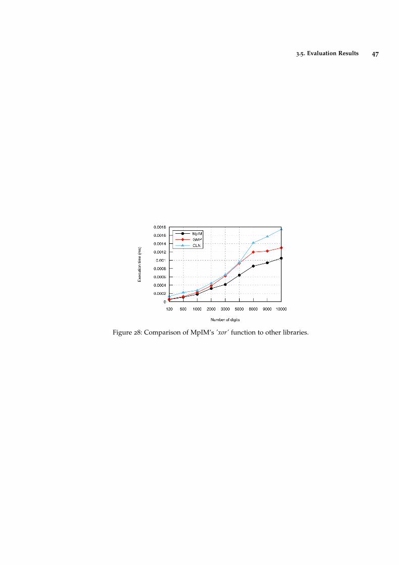
3.5. Evaluation Results 47

Figure 28: Comparison of MpIM’s ’xor’ function to other libraries.

4

T H E Q I A O ’ S J A C O B I M E T H O D

In this chapter we identify several bottlenecks of the Qiao’s Jacobi method and propose ef-ficient solutions to minimize them. Our final implementation is described in the Algorithm4.1. While we identify a particular bottleneck we indicate the correspondent lines in theproposed version. All the proposed implementations of this chapter are included in theLattBRed module.

We start to inline the function Lagrange in the main algorithm. It allows to make changesdirectly in the matrix Z of the main function. To inline the Lagrange function we assumethat Z′ of the Lagrange function and Z of the main function are the same. With it, the matrixinitialization in the line 13 is removed and the matrix multiplication in the line 7 is avoided,since the same result is produced in the line 23.

The Qiao’s Jacobi method is highly parallel due to the majority of matrix computations,which makes it an opportunity to exploit it in parallel systems. We will see in this chapterthat this statement may be risky. With a closer look to the Algorithm 2.10 we identifiedopportunities to avoid unnecessary computation on integral matrix multiplications. Thisopportunity appears in the Lagrange function when we analysis the output of a multiplica-tion of any square matrix M by Z or ZT. We noticed that the multiplication MZ outcomeswith almost the same result as matrix M, where it subtracts the column i by the multipli-cation of q by the column j. The same happens in the matrix multiplication ZTM, whichcomputes rows instead of columns. Thus, it is possible to substitute heavy integral matrixmultiplication by a row and column computations. Therefore, the matrix Z of the Lagrangefunction is not needed because the computations are done directly in matrices G and Z′.To implement this improvement the line 11 is substituted by G(i:) = G(i:)− q×G(j:) andG(:i) = G(:i)− q ×G(:j) plus the column and row swaps, and the line 12 is substitutedby Z(i:) = Z(i:)− q× Z(j:) plus a row swap. The functions Row Column Computationsand Row Computations of the Algorithm 4.1 intent to represent these computations on amatrix. If q is 0, these function have no effect. For comparison purposes, we consider theQiao’s Jacobi method with this improvement as the base version.

After performing the functions Row Column Computations and Row Computations, itneeds to perform swap of the row and column i and j in order to maintain the algorithm

48

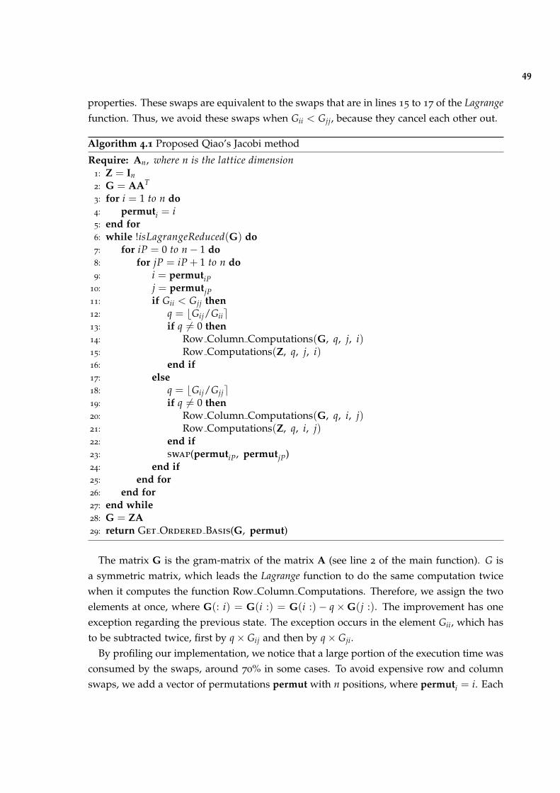
49

properties. These swaps are equivalent to the swaps that are in lines 15 to 17 of the Lagrangefunction. Thus, we avoid these swaps when Gii < Gjj, because they cancel each other out.

Algorithm 4.1 Proposed Qiao’s Jacobi method

Require: An, where n is the lattice dimension1: Z = In2: G = AAT

3: for i = 1 to n do4: permuti = i5: end for6: while !isLagrangeReduced(G) do7: for iP = 0 to n− 1 do8: for jP = iP + 1 to n do9: i = permutiP

10: j = permutjP11: if Gii < Gjj then12: q = bGij/Giie13: if q 6= 0 then14: Row Column Computations(G, q, j, i)15: Row Computations(Z, q, j, i)16: end if17: else18: q = bGij/Gjje19: if q 6= 0 then20: Row Column Computations(G, q, i, j)21: Row Computations(Z, q, i, j)22: end if23: swap(permutiP, permutjP)24: end if25: end for26: end for27: end while28: G = ZA29: return Get Ordered Basis(G, permut)

The matrix G is the gram-matrix of the matrix A (see line 2 of the main function). G isa symmetric matrix, which leads the Lagrange function to do the same computation twicewhen it computes the function Row Column Computations. Therefore, we assign the twoelements at once, where G(: i) = G(i :) = G(i :)− q×G(j :). The improvement has oneexception regarding the previous state. The exception occurs in the element Gii, which hasto be subtracted twice, first by q× Gij and then by q× Gji.

By profiling our implementation, we notice that a large portion of the execution time wasconsumed by the swaps, around 70% in some cases. To avoid expensive row and columnswaps, we add a vector of permutations permut with n positions, where permuti = i. Each

50

position indicates the index of a particular vector in the matrices G and Z. Thus, we justneed to swap the values of the vector of permutations to maintain the algorithm properties.To implement it, we add the lines 3 and 4 to initialize the vector, the lines 9 and 10 to getthe correspondent vector indexes and the swap of line 23.

The S. Qiao represents the basis vectors in the different columns of the matrix. Dueto better data access patterns in C++, we represent the basis vectors in rows instead ofcolumns.

After all these improvements, we were capable to achieve performances way more attrac-tive than the original algorithm. We implemented two versions of the Algorithm 4.1, (i)a MP version to reduce GM bases, and (ii) a version with primitive data types to reduceAjtai-type bases.

4.0.1 Vectorization

The second version uses primitive data types. Thus, we were able to exploit some featuresof current processor architectures, such as SIMD extensions. The following parts of thealgorithm were improved:

• Gram-matrix computation (AAT);

• Row Computations function;

• Matrix multiplication (AZ).

The Gram-matrix computation was improved in several ways. Since the Gram-matrixis symmetric it only computes the inner products of the upper-triangular matrix and thelower-triangular is assigned with the previous results. Then, to allow the use of SIMDinstructions we add padding in the end of each vector to guarantee the data alignment andthe memory accesses are always made in contiguous memory, except in the lower-triangularassignments.

The function Row Computations computes operations through the vector elements. Sincethe vector’s data was aligned in the previous optimization, we just add Intel intrinsics.

It is impossible to efficiently vectorize the standard matrix multiplication algorithm dueto the memory access patterns. There is vector instructions that gather the data, howeverthe Intel warning about huge time penalties. To efficiently vectorize it, the matrix multi-plication’s cycles were reordered in a cache-friendly access pattern, allowing contiguousmemory accesses (stride-1).

Speedup =Original Execution TimeExpected Execution Time

=100%

(100%− 30.34%) + ( 30.34%8 )

(13)

51

Although vectorization may lead to significative speedups, it is crucial to measure thetheoretical speedup before initiating the implementation. The identified parts in the codeconsume 9.5%, 0.84% and 20% of the execution time, respectively, making a total of 30.34%.Taking in account that each SIMD instruction operates on 8 integer elements at once (inthis case study), it is expected a theoretical speedup of 1.36. Equation 13 shows how thespeedup was computed, where we inserted the bold face numbers on the equation. Theused Intel intrinsics are:

• mm256 load si256;

• mm256 store si256;

• mm256 set1 epi32;

• mm256 mullo epi32;

• mm256 add epi32;

• mm256 sub epi32;

4.0.2 Evaluation Results

This section measures the impact of most important improvements proposed to the Algo-rithm 2.10. We analysed the two implemented versions and compared them with the LLLalgorithm.

It is not possible to compare the execution time of our implementations and the an-nounced times in Qiao (2012) due to several reasons. First, some of our implementationsuse integer MP arithmetic, and S. Qiao does not indicate which data type is using in hisexperiment. However, floating-point arithmetic is referred in [Jeremic and Qiao (2014)].Secondly, S. Qiao generates random lattice bases but did not indicate which type of latticebasis he performed the experiments. S. Qiao obtained a maximal number of 8 sweeps, how-ever GM bases require more sweeps than the expected. The number of sweeps is illustratedin Figure 33. The reason why it performs so many sweeps is because GM bases are veryill-conditioned.

Figure 29 compares the LLL algorithm with the ’extended doubles’ data type from theNTL and three MP implementations of the Qiao’s Jacobi method. The ’MP Qiao Base’ isthe base version of the Algorithm 2.10, where we removed almost every matrix multiplica-tions. The ’MP Qiao w/ Swaps’ does not implement the proposed improvement that avoidsintegral matrix swaps, and the ’MP Qiao’ implements all the proposed improvements forMP arithmetic. The experiment shows that after all the improvements, the ’MP Qiao’ imple-mentation is about 3 times faster than the base version, and the last improvement speed up

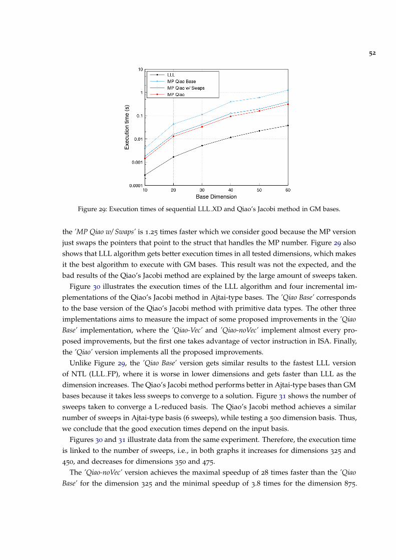
52

Figure 29: Execution times of sequential LLL XD and Qiao’s Jacobi method in GM bases.

the ’MP Qiao w/ Swaps’ is 1.25 times faster which we consider good because the MP versionjust swaps the pointers that point to the struct that handles the MP number. Figure 29 alsoshows that LLL algorithm gets better execution times in all tested dimensions, which makesit the best algorithm to execute with GM bases. This result was not the expected, and thebad results of the Qiao’s Jacobi method are explained by the large amount of sweeps taken.

Figure 30 illustrates the execution times of the LLL algorithm and four incremental im-plementations of the Qiao’s Jacobi method in Ajtai-type bases. The ’Qiao Base’ correspondsto the base version of the Qiao’s Jacobi method with primitive data types. The other threeimplementations aims to measure the impact of some proposed improvements in the ’QiaoBase’ implementation, where the ’Qiao-Vec’ and ’Qiao-noVec’ implement almost every pro-posed improvements, but the first one takes advantage of vector instruction in ISA. Finally,the ’Qiao’ version implements all the proposed improvements.

Unlike Figure 29, the ’Qiao Base’ version gets similar results to the fastest LLL versionof NTL (LLL FP), where it is worse in lower dimensions and gets faster than LLL as thedimension increases. The Qiao’s Jacobi method performs better in Ajtai-type bases than GMbases because it takes less sweeps to converge to a solution. Figure 31 shows the number ofsweeps taken to converge a L-reduced basis. The Qiao’s Jacobi method achieves a similarnumber of sweeps in Ajtai-type basis (6 sweeps), while testing a 500 dimension basis. Thus,we conclude that the good execution times depend on the input basis.

Figures 30 and 31 illustrate data from the same experiment. Therefore, the execution timeis linked to the number of sweeps, i.e., in both graphs it increases for dimensions 325 and450, and decreases for dimensions 350 and 475.

The ’Qiao-noVec’ version achieves the maximal speedup of 28 times faster than the ’QiaoBase’ for the dimension 325 and the minimal speedup of 3.8 times for the dimension 875.

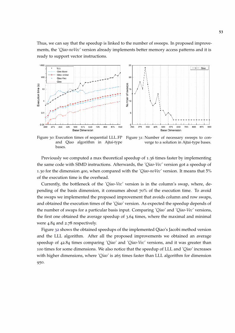
53

Thus, we can say that the speedup is linked to the number of sweeps. In proposed improve-ments, the ’Qiao-noVec’ version already implements better memory access patterns and it isready to support vector instructions.

Figure 30: Execution times of sequential LLL FPand Qiao algorithm in Ajtai-typebases.

Figure 31: Number of necessary sweeps to con-verge to a solution in Ajtai-type bases.

Previously we computed a max theoretical speedup of 1.36 times faster by implementingthe same code with SIMD instructions. Afterwards, the ’Qiao-Vec’ version got a speedup of1.30 for the dimension 400, when compared with the ’Qiao-noVec’ version. It means that 5%of the execution time is the overhead.

Currently, the bottleneck of the ’Qiao-Vec’ version is in the column’s swap, where, de-pending of the basis dimension, it consumes about 70% of the execution time. To avoidthe swaps we implemented the proposed improvement that avoids column and row swaps,and obtained the execution times of the ’Qiao’ version. As expected the speedup depends ofthe number of swaps for a particular basis input. Comparing ’Qiao’ and ’Qiao-Vec’ versions,the first one obtained the average speedup of 3.64 times, where the maximal and minimalwere 4.84 and 2.78 respectively.

Figure 32 shows the obtained speedups of the implemented Qiao’s Jacobi method versionand the LLL algorithm. After all the proposed improvements we obtained an averagespeedup of 42.84 times comparing ’Qiao’ and ’Qiao-Vec’ versions, and it was greater than100 times for some dimensions. We also notice that the speedup of LLL and ’Qiao’ increaseswith higher dimensions, where ’Qiao’ is 265 times faster than LLL algorithm for dimension950.

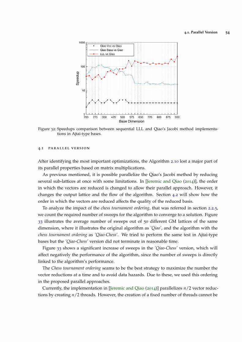
4.1. Parallel Version 54

Figure 32: Speedups comparison between sequential LLL and Qiao’s Jacobi method implementa-tions in Ajtai-type bases.

4.1 parallel version

After identifying the most important optimizations, the Algorithm 2.10 lost a major part ofits parallel properties based on matrix multiplications.

As previous mentioned, it is possible parallelize the Qiao’s Jacobi method by reducingseveral sub-lattices at once with some limitations. In [Jeremic and Qiao (2014)], the orderin which the vectors are reduced is changed to allow their parallel approach. However, itchanges the output lattice and the flow of the algorithm. Section 4.2 will show how theorder in which the vectors are reduced affects the quality of the reduced basis.

To analyze the impact of the chess tournament ordering, that was referred in section 2.2.5,we count the required number of sweeps for the algorithm to converge to a solution. Figure33 illustrates the average number of sweeps out of 50 different GM lattices of the samedimension, where it illustrates the original algorithm as ’Qiao’, and the algorithm with thechess tournament ordering as ’Qiao-Chess’. We tried to perform the same test in Ajtai-typebases but the ’Qiao-Chess’ version did not terminate in reasonable time.

Figure 33 shows a significant increase of sweeps in the ’Qiao-Chess’ version, which willaffect negatively the performance of the algorithm, since the number of sweeps is directlylinked to the algorithm’s performance.

The Chess tournament ordering seams to be the best strategy to maximize the number thevector reductions at a time and to avoid data hazards. Due to these, we used this orderingin the proposed parallel approaches.

Currently, the implementation in [Jeremic and Qiao (2014)] parallelizes n/2 vector reduc-tions by creating n/2 threads. However, the creation of a fixed number of threads cannot be

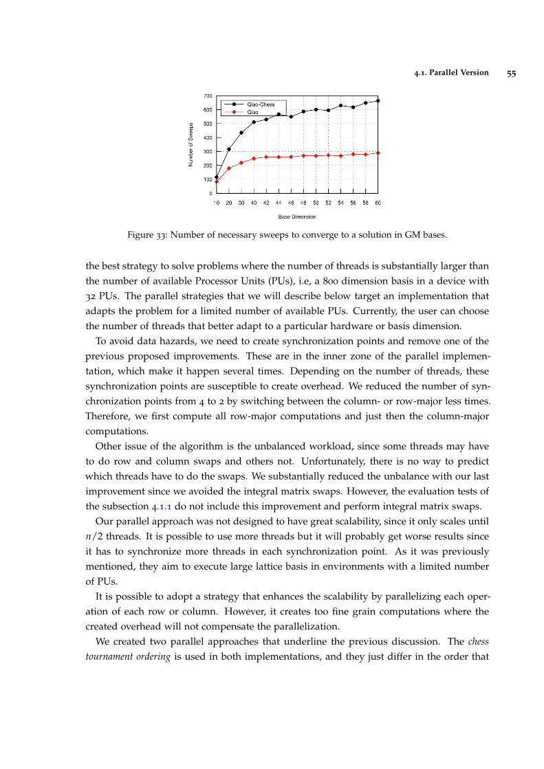
4.1. Parallel Version 55

Figure 33: Number of necessary sweeps to converge to a solution in GM bases.

the best strategy to solve problems where the number of threads is substantially larger thanthe number of available Processor Units (PUs), i.e, a 800 dimension basis in a device with32 PUs. The parallel strategies that we will describe below target an implementation thatadapts the problem for a limited number of available PUs. Currently, the user can choosethe number of threads that better adapt to a particular hardware or basis dimension.

To avoid data hazards, we need to create synchronization points and remove one of theprevious proposed improvements. These are in the inner zone of the parallel implemen-tation, which make it happen several times. Depending on the number of threads, thesesynchronization points are susceptible to create overhead. We reduced the number of syn-chronization points from 4 to 2 by switching between the column- or row-major less times.Therefore, we first compute all row-major computations and just then the column-majorcomputations.

Other issue of the algorithm is the unbalanced workload, since some threads may haveto do row and column swaps and others not. Unfortunately, there is no way to predictwhich threads have to do the swaps. We substantially reduced the unbalance with our lastimprovement since we avoided the integral matrix swaps. However, the evaluation tests ofthe subsection 4.1.1 do not include this improvement and perform integral matrix swaps.

Our parallel approach was not designed to have great scalability, since it only scales untiln/2 threads. It is possible to use more threads but it will probably get worse results sinceit has to synchronize more threads in each synchronization point. As it was previouslymentioned, they aim to execute large lattice basis in environments with a limited numberof PUs.

It is possible to adopt a strategy that enhances the scalability by parallelizing each oper-ation of each row or column. However, it creates too fine grain computations where thecreated overhead will not compensate the parallelization.

We created two parallel approaches that underline the previous discussion. The chesstournament ordering is used in both implementations, and they just differ in the order that

4.1. Parallel Version 56

all n/2 vector reductions are done. The first approach is divided in two parts, whereit performs all row-major order computations in first place, and just then it performs allcolumn-major order computations. Each part is within a for-cycle that performs all n/2pair combinations. To not compute the value of the variable q of each pair combinationin each for-cycle, we cache its value in the first for-cycle into an array and reuse it in thesecond one.

The second approach parallelizes x of the n/2 pair combinations at once, by performingall row and column computations. To avoid data hazards, we implement synchronizationpoints between the row and column computation and in the end of the column computa-tion.

We used OpenMP to parallelize both implementations. In the first approach the syn-chronization points were implemented with the inherit properties of the directive ’#pragmaomp for’, which already implements a barrier. In the second approach the synchronizationpoints are implemented with the directive ’#pragma omp barrier’.

The first approach has the advantage of computing all row- or column-major order com-putations without synchronization points what could lead to better performances. However,it has time penalties to access the stored data on the second for-cycle. This approach leadsto a higher memory consumption.

Unlike the first approach, the second one has a lower memory consumption, since it doesnot have to memoize data. However it may have to deal with more synchronization points,i.e., if the number of threads is lower than n/2, it has to do all the iteration more than once.

4.1.1 Evaluation Results

Figures 34 and 35 illustrate how the execution time changed with the increase of the numberof threads. It uses GM lattice bases with the dimension between 10 and 60 and shows theaverage value out of 50 different bases. Depending in the lattice dimension, both figuresdo not illustrate the value for greater number of threads, i.e., dimension 10 with 16 threads.It happens because the execution times got worse because the number of threads is greaterthan n/2.

In every dimension of both figures, the test with 1 thread gets the best execution time. Itmeans that overhead created to parallelize the algorithm takes a large portion of the finalexecution time, which means that the parallelization does not compensate for GM baseswhere it is used MP.

Note that these approaches may have different results in implementations with primitivedata types, where it deals with different memory access patterns.

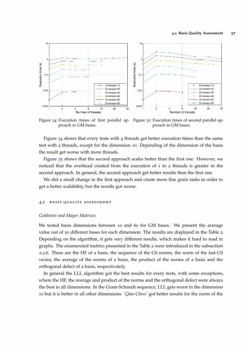
4.2. Basis Quality Assessment 57

Figure 34: Execution times of first parallel ap-proach in GM bases.

Figure 35: Execution times of second parallel ap-proach in GM bases.

Figure 34 shows that every tests with 4 threads get better execution times than the sametest with 2 threads, except for the dimension 10. Depending of the dimension of the basisthe result get worse with more threads.

Figure 35 shows that the second approach scales better than the first one. However, wenoticed that the overhead created from the execution of 1 to 2 threads is greater in thesecond approach. In general, the second approach get better results than the first one.

We did a small change in the first approach and create more fine grain tasks in order toget a better scalability, but the results got worse.

4.2 basis quality assessment

Goldstein and Mayer Matrices

We tested basis dimensions between 10 and 60 for GM bases. We present the averagevalue out of 50 different bases for each dimension. The results are displayed in the Table 2.Depending on the algorithm, it gets very different results, which makes it hard to read ingraphs. The enumerated metrics presented in the Table 2 were introduced in the subsection2.2.6. These are the HF of a basis, the sequence of the GS norms, the norm of the last GSvector, the average of the norms of a basis, the product of the norms of a basis and theorthogonal defect of a basis, respectivately.

In general the LLL algorithm got the best results for every tests, with some exceptions,where the HF, the average and product of the norms and the orthogonal defect were alwaysthe best in all dimensions. In the Gram-Schmidt sequence, LLL gets worst in the dimension10 but it is better in all other dimensions. ’Qiao-Chess’ got better results for the norm of the

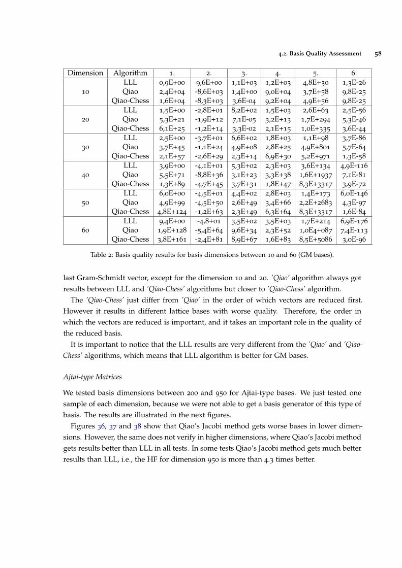
4.2. Basis Quality Assessment 58

Dimension Algorithm 1. 2. 3. 4. 5. 6.LLL 0,9E+00 9,6E+00 1,1E+03 1,2E+03 4,8E+30 1,3E-26

10 Qiao 2,4E+04 -8,6E+03 1,4E+00 9,0E+04 3,7E+58 9,8E-25

Qiao-Chess 1,6E+04 -8,3E+03 3,6E-04 9,2E+04 4,9E+56 9,8E-25

LLL 1,5E+00 -2,8E+01 8,2E+02 1,5E+03 2,6E+63 2,5E-56

20 Qiao 5,3E+21 -1,9E+12 7,1E-05 3,2E+13 1,7E+294 5,3E-46

Qiao-Chess 6,1E+25 -1,2E+14 3,3E-02 2,1E+15 1,0E+335 3,6E-44

LLL 2,5E+00 -3,7E+01 6,6E+02 1,8E+03 1,1E+98 3,7E-86

30 Qiao 3,7E+45 -1,1E+24 4,9E+08 2,8E+25 4,9E+801 5,7E-64

Qiao-Chess 2,1E+57 -2,6E+29 2,3E+14 6,9E+30 5,2E+971 1,3E-58

LLL 3,9E+00 -4,1E+01 5,3E+02 2,3E+03 3,6E+134 4,9E-116

40 Qiao 5,5E+71 -8,8E+36 3,1E+23 3,3E+38 1,6E+1937 7,1E-81

Qiao-Chess 1,3E+89 -4,7E+45 3,7E+31 1,8E+47 8,3E+3317 3,9E-72

LLL 6,0E+00 -4,5E+01 4,4E+02 2,8E+03 1,4E+173 6,0E-146

50 Qiao 4,9E+99 -4,5E+50 2,6E+49 3,4E+66 2,2E+2683 4,3E-97

Qiao-Chess 4,8E+124 -1,2E+63 2,3E+49 6,3E+64 8,3E+3317 1,6E-84

LLL 9,4E+00 -4,8+01 3,5E+02 3,5E+03 1,7E+214 6,9E-176

60 Qiao 1,9E+128 -5,4E+64 9,6E+34 2,3E+52 1,0E4+087 7,4E-113

Qiao-Chess 3,8E+161 -2,4E+81 8,9E+67 1,6E+83 8,5E+5086 3,0E-96

Table 2: Basis quality results for basis dimensions between 10 and 60 (GM bases).

last Gram-Schmidt vector, except for the dimension 10 and 20. ’Qiao’ algorithm always gotresults between LLL and ’Qiao-Chess’ algorithms but closer to ’Qiao-Chess’ algorithm.

The ’Qiao-Chess’ just differ from ’Qiao’ in the order of which vectors are reduced first.However it results in different lattice bases with worse quality. Therefore, the order inwhich the vectors are reduced is important, and it takes an important role in the quality ofthe reduced basis.

It is important to notice that the LLL results are very different from the ’Qiao’ and ’Qiao-Chess’ algorithms, which means that LLL algorithm is better for GM bases.

Ajtai-type Matrices

We tested basis dimensions between 200 and 950 for Ajtai-type bases. We just tested onesample of each dimension, because we were not able to get a basis generator of this type ofbasis. The results are illustrated in the next figures.

Figures 36, 37 and 38 show that Qiao’s Jacobi method gets worse bases in lower dimen-sions. However, the same does not verify in higher dimensions, where Qiao’s Jacobi methodgets results better than LLL in all tests. In some tests Qiao’s Jacobi method gets much betterresults than LLL, i.e., the HF for dimension 950 is more than 4.3 times better.

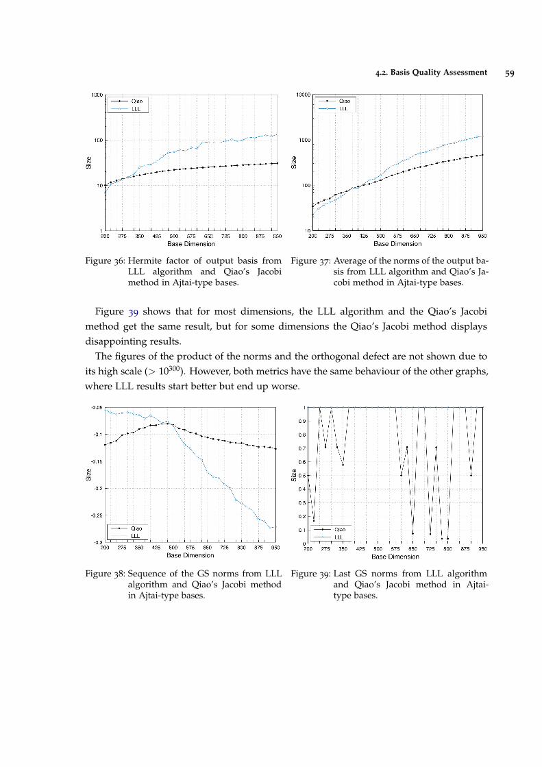
4.2. Basis Quality Assessment 59

Figure 36: Hermite factor of output basis fromLLL algorithm and Qiao’s Jacobimethod in Ajtai-type bases.

Figure 37: Average of the norms of the output ba-sis from LLL algorithm and Qiao’s Ja-cobi method in Ajtai-type bases.

Figure 39 shows that for most dimensions, the LLL algorithm and the Qiao’s Jacobimethod get the same result, but for some dimensions the Qiao’s Jacobi method displaysdisappointing results.

The figures of the product of the norms and the orthogonal defect are not shown due toits high scale (> 10300). However, both metrics have the same behaviour of the other graphs,where LLL results start better but end up worse.

Figure 38: Sequence of the GS norms from LLLalgorithm and Qiao’s Jacobi methodin Ajtai-type bases.

Figure 39: Last GS norms from LLL algorithmand Qiao’s Jacobi method in Ajtai-type bases.

5

B K Z , L L L A N D Q I A O ’ S J A C O B I M E T H O D

This chapter explores possible parallel approaches of well known lattice basis reductionalgorithms such as LLL and BKZ. In addition, a variant of the BKZ algorithm in whichthe LLL algorithm was replaced by the Qiao’s Jacobi method was implemented, and it wasassessed the basis quality output of combining the Qiao’s Jacobi method with LLL and BKZalgorithms. All the proposed implementations of this chapter are included in the LattBRedmodule.

5.1 towards parallel approaches

5.1.1 Parallel LLL algorithm

We implemented a floating-point version of the Algorithm 2.8 to do experiments in GMbases. To ensure the correctness of the implementation we compared its basis output andthe output of the ’LLL XD’ function of the NTL. However it did not work as expected, andto obtain the same output we had to compute the GS coefficients and norm after the size-reduction. The computation of the GS coefficients with the size-reduced vector minimizeprecision errors.

The first LLL implementation uses the NTL to handle with MP arithmetic. However, ittook more time than expected in the conversion of the MP number to the double datatype,where the GMP’s conversion is more efficient. This led to a second implementation wherewe used the GMP to handle with MP arithmetic.

By profiling our implementation, we noticed that 35% of the execution time is consumedby the computation of the GS coefficients and norms and 62% by the size-reduction. There-fore, it is imperative to parallelize these parts of the algorithm in order to get more perfor-mance.

After look into the GS algorithm we found an opportunity to parallelize this procedureby computing the inner products in parallel. This procedure is called several times duringthe algorithm execution, thus it is not a good approach to create and destroy a new parallelzone every time that the procedure is called, since it is one of the heaviest calls in paral-

60

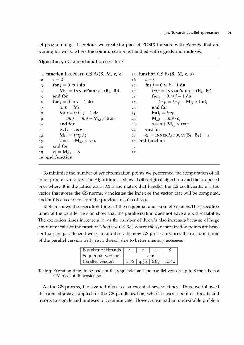
5.1. Towards parallel approaches 61

lel programming. Therefore, we created a pool of POSIX threads, with pthreads, that arewaiting for work, where the communication is handled with signals and mutexes.

Algorithm 5.1 Gram-Schmidt process for k

1: function Proposed GS Bk(B, M, c, k)2: s = 03: for j = 0 to k do4: Mk,j = InnerProduct(Bk, Bj)5: end for6: for j = 0 to k− 1 do7: tmp = Mk,j8: for i = 0 to j− 1 do9: tmp = tmp−Mj,i × bufi

10: end for11: bufj = tmp12: Mk,j = tmp/cj13: s = s + Mk,j × tmp14: end for15: ck = Mk,k − s16: end function

17: function GS Bk(B, M, c, k)18: s = 019: for j = 0 to k− 1 do20: tmp = InnerProduct(Bk, Bj)21: for i = 0 to j− 1 do22: tmp = tmp−Mj,i × bufi23: end for24: bufj = tmp25: Mk,j = tmp/cj26: s = s + Mk,j × tmp27: end for28: ck = InnerProduct(Bk, Bk) − s29: end function30:31:

To minimize the number of synchronization points we performed the computation of allinner products at once. The Algorithm 5.1 shows both original algorithm and the proposedone, where B is the lattice basis, M is the matrix that handles the GS coefficients, c is thevector that stores the GS norms, k indicates the index of the vector that will be computed,and buf is a vector to store the previous results of tmp.

Table 3 shows the execution times of the sequential and parallel versions.The executiontimes of the parallel version show that the parallelization does not have a good scalability.The execution times increase a lot as the number of threads also increases because of hugeamount of calls of the function ’Proposed GS Bk’, where the synchronization points are heav-ier than the parallelized work. In addition, the new GS process reduces the execution timeof the parallel version with just 1 thread, due to better memory accesses.

Number of threads 1 2 4 8

Sequential version 2.16

Parallel version 1.86 4.50 6.89 10.62

Table 3: Execution times in seconds of the sequential and the parallel version up to 8 threads in aGM basis of dimension 50.

As the GS process, the size-redution is also executed several times. Thus, we followedthe same strategy adopted for the GS parallelization, where it uses a pool of threads andresorts to signals and mutexes to communicate. However, we had an undesirable problem

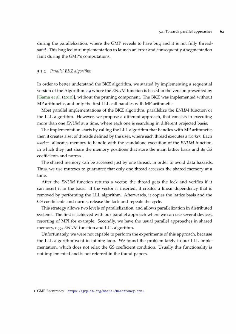
5.1. Towards parallel approaches 62

during the parallelization, where the GMP reveals to have bug and it is not fully thread-safe1. This bug led our implementation to launch an error and consequently a segmentationfault during the GMP’s computations.

5.1.2 Parallel BKZ algorithm

In order to better understand the BKZ algorithm, we started by implementing a sequentialversion of the Algorithm 2.9 where the ENUM function is based in the version presented by[Gama et al. (2010)], without the pruning component. The BKZ was implemented withoutMP arithmetic, and only the first LLL call handles with MP arithmetic.

Most parallel implementations of the BKZ algorithm, parallelize the ENUM function orthe LLL algorithm. However, we propose a different approach, that consists in executingmore than one ENUM at a time, where each one is searching in different projected basis.

The implementation starts by calling the LLL algorithm that handles with MP arithmetic,then it creates a set of threads defined by the user, where each thread executes a worker. Eachworker allocates memory to handle with the standalone execution of the ENUM function,in which they just share the memory positions that store the main lattice basis and its GScoefficients and norms.

The shared memory can be accessed just by one thread, in order to avoid data hazards.Thus, we use mutexes to guarantee that only one thread accesses the shared memory at atime.

After the ENUM function returns a vector, the thread gets the lock and verifies if itcan insert it in the basis. If the vector is inserted, it creates a linear dependency that isremoved by performing the LLL algorithm. Afterwards, it copies the lattice basis and theGS coefficients and norms, release the lock and repeats the cycle.

This strategy allows two levels of parallelization, and allows parallelization in distributedsystems. The first is achieved with our parallel approach where we can use several devices,resorting of MPI for example. Secondly, we have the usual parallel approaches in sharedmemory, e.g., ENUM function and LLL algorithm.

Unfortunately, we were not capable to perform the experiments of this approach, becausethe LLL algorithm went in infinite loop. We found the problem lately in our LLL imple-mentation, which does not relax the GS coefficient condition. Usually this functionality isnot implemented and is not referred in the found papers.

1 GMP Reentrancy - https://gmplib.org/manual/Reentrancy.html

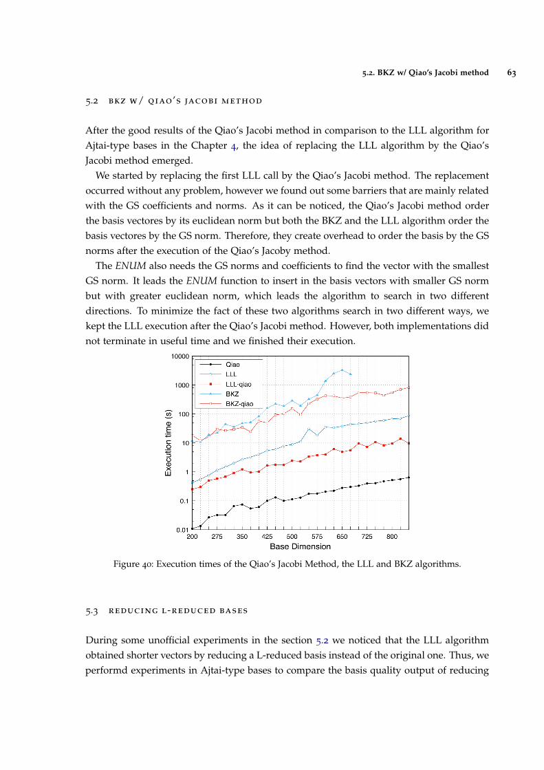
5.2. BKZ w/ Qiao’s Jacobi method 63

5.2 bkz w/ qiao’s jacobi method

After the good results of the Qiao’s Jacobi method in comparison to the LLL algorithm forAjtai-type bases in the Chapter 4, the idea of replacing the LLL algorithm by the Qiao’sJacobi method emerged.

We started by replacing the first LLL call by the Qiao’s Jacobi method. The replacementoccurred without any problem, however we found out some barriers that are mainly relatedwith the GS coefficients and norms. As it can be noticed, the Qiao’s Jacobi method orderthe basis vectores by its euclidean norm but both the BKZ and the LLL algorithm order thebasis vectores by the GS norm. Therefore, they create overhead to order the basis by the GSnorms after the execution of the Qiao’s Jacoby method.

The ENUM also needs the GS norms and coefficients to find the vector with the smallestGS norm. It leads the ENUM function to insert in the basis vectors with smaller GS normbut with greater euclidean norm, which leads the algorithm to search in two differentdirections. To minimize the fact of these two algorithms search in two different ways, wekept the LLL execution after the Qiao’s Jacobi method. However, both implementations didnot terminate in useful time and we finished their execution.

Figure 40: Execution times of the Qiao’s Jacobi Method, the LLL and BKZ algorithms.

5.3 reducing l-reduced bases

During some unofficial experiments in the section 5.2 we noticed that the LLL algorithmobtained shorter vectors by reducing a L-reduced basis instead of the original one. Thus, weperformd experiments in Ajtai-type bases to compare the basis quality output of reducing

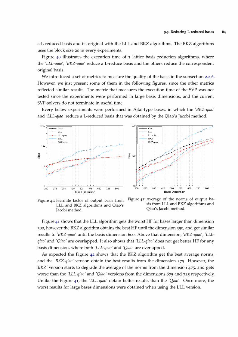
5.3. Reducing L-reduced bases 64

a L-reduced basis and its original with the LLL and BKZ algorithms. The BKZ algorithmsuses the block size 20 in every experiments.

Figure 40 illustrates the execution time of 3 lattice basis reduction algorithms, wherethe ’LLL-qiao’, ’BKZ-qiao’ reduce a L-reduce basis and the others reduce the correspondentoriginal basis.

We introduced a set of metrics to measure the quality of the basis in the subsection 2.2.6.However, we just present some of them in the following figures, since the other metricsreflected similar results. The metric that measures the execution time of the SVP was nottested since the experiments were performed in large basis dimensions, and the currentSVP-solvers do not terminate in useful time.

Every below experiments were performed in Ajtai-type bases, in which the ’BKZ-qiao’and ’LLL-qiao’ reduce a L-reduced basis that was obtained by the Qiao’s Jacobi method.

Figure 41: Hermite factor of output basis fromLLL and BKZ algorithms and Qiao’sJacobi method.

Figure 42: Average of the norms of output ba-sis from LLL and BKZ algorithms andQiao’s Jacobi method.

Figure 41 shows that the LLL algorithm gets the worst HF for bases larger than dimension300, however the BKZ algorithm obtains the best HF until the dimension 350, and get similarresults to ’BKZ-qiao’ until the basis dimension 600. Above that dimension, ’BKZ-qiao’, ’LLL-qiao’ and ’Qiao’ are overlapped. It also shows that ’LLL-qiao’ does not get better HF for anybasis dimension, where both ’LLL-qiao’ and ’Qiao’ are overlapped.

As expected the Figure 42 shows that the BKZ algorithm get the best average norms,and the ’BKZ-qiao’ version obtain the best results from the dimension 375. However, the’BKZ’ version starts to degrade the average of the norms from the dimension 475, and getsworse than the ’LLL-qiao’ and ’Qiao’ versions from the dimensions 675 and 725 respectively.Unlike the Figure 41, the ’LLL-qiao’ obtain better results than the ’Qiao’. Once more, theworst results for large bases dimensions were obtained when using the LLL version.

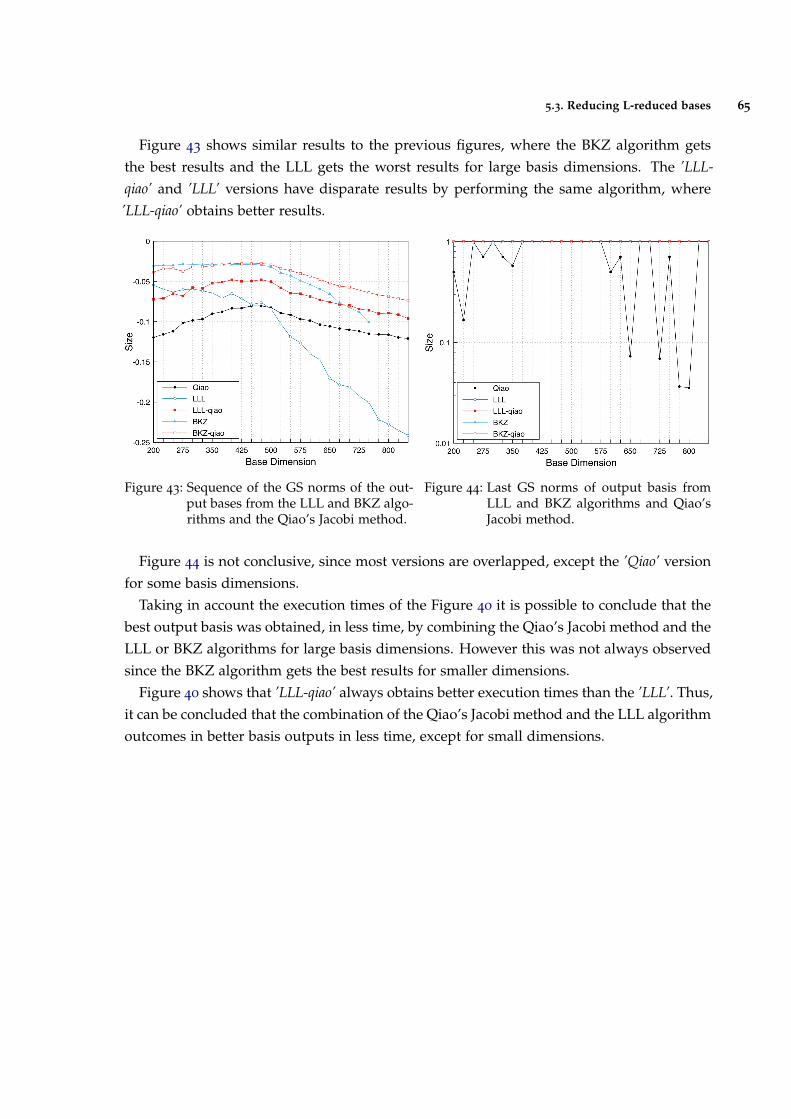
5.3. Reducing L-reduced bases 65

Figure 43 shows similar results to the previous figures, where the BKZ algorithm getsthe best results and the LLL gets the worst results for large basis dimensions. The ’LLL-qiao’ and ’LLL’ versions have disparate results by performing the same algorithm, where’LLL-qiao’ obtains better results.

Figure 43: Sequence of the GS norms of the out-put bases from the LLL and BKZ algo-rithms and the Qiao’s Jacobi method.

Figure 44: Last GS norms of output basis fromLLL and BKZ algorithms and Qiao’sJacobi method.

Figure 44 is not conclusive, since most versions are overlapped, except the ’Qiao’ versionfor some basis dimensions.

Taking in account the execution times of the Figure 40 it is possible to conclude that thebest output basis was obtained, in less time, by combining the Qiao’s Jacobi method and theLLL or BKZ algorithms for large basis dimensions. However this was not always observedsince the BKZ algorithm gets the best results for smaller dimensions.

Figure 40 shows that ’LLL-qiao’ always obtains better execution times than the ’LLL’. Thus,it can be concluded that the combination of the Qiao’s Jacobi method and the LLL algorithmoutcomes in better basis outputs in less time, except for small dimensions.

6

C O N C L U S I O N S & F U T U R E W O R K

The dissertation is focused on lattice basis reduction algorithms and MP arithmetic, thatis in some case studies one of its key requirements. Therefore, it is expected that thedeveloped material creates value to the scientific community by proposing more efficientimplementations or algorithms, and scrutinizing related issues.

An efficient integer MP module was developed that took advantage of the late microar-chitectures for logical and shifts operations by using vector instructions. These operationsobtained better execution times than the correspondent operation of the most known MPlibraries.

Although the addition is one of the simplest operations, it plays a key role and deservedan investment to study several approaches. A vectorized version of this function in AVX-2was implemented, without obtaining good performances. The poor execution time followsfrom the dependencies in the MP addition. To obtain better performances we implementedan assembly version that does two additions sequentially avoiding one overflow test percycle. This last version obtained similar execution times compared to the other libraries,and in some cases it got the best execution time.

Less time was invested in the subtraction algorithm, which resulted in execution timesnot so good as expected. However, it is possible to implement the same assembly approachtaken for the addition algorithm, which will result in more appealing execution times.

The MpIM’s multiplication obtained better execution times than the NTL library untila certain number of digits. It happened because NTL library implements algorithms rec-ommended for very large MP numbers, and we just implemented the long multiplicationand the Karatsuba algorithms. However, the execution times of our implementations wereworse than the execution times of the GMP and CLN libraries. Therefore, further researchcan be done to improve the MpIM’s multiplication. The long multiplication can be im-proved by loop-unrolling several primitive multiplications in its intermediate steps, andby keeping good memory access patterns. By improving the long multiplication, it willautomatically reflect in better execution times of the Karatsuba algorithm.

Due to time constraints, the MpIM’s division had execution times that were not theexpected, and it needs to be improved in follow researches.

66

67

Note that is hard to get better execution times than libraries such as GMP, where functionslike addition, subtraction and the multiplication basecase have assembly versions for certainCPU that give significant speedups, mainly through avoiding function call overheads1.

S. Qiao claimed that its Jacobi method has inherit parallel properties due to the requiredmatrix computations. However, a good implementation of its algorithm must rely its com-putations in the Gram-Matrix. It removes most matrix multiplications of the algorithm,and its inherit parallel properties fade out. The dissertation presents a novel sequentialimplementation of the Qiao’s Jacobi method that gets better results than the original imple-mentation presented in [Qiao (2012)]. To accomplish good performances we avoided severalcomputations and memory swaps and we developed two versions of this implementation:a MP version to handle GM bases and a version with primitive data types to handle Ajtai-type bases. Both versions have good have good speedups, but the version with primitivedata types stands out with maximal speedups of 114 times and it reached speedups of 20

times with large basis dimensions.The Qiao’s Jacobi method does not performs well in GM bases, since these bases are

very ill-conditioned, which leads the algorithm to make many sweeps, degrading its overallperformance. Comparing its performance with the LLL algorithm, it takes longer to executeand its basis output is worse than the LLL algorithm for GM bases.

Unlike the previous version, the version with primitive data types performs well in Ajtai-type bases, and takes less time to execute than the LLL algorithm and the basis outputsare better than the LLL algorithm. The good execution times are related to the number ofsweeps that the algorithm takes to get a L-reduced basis.

We also proposed two MP parallel approaches of the Qiao’s Jacobi method that is bestsuited to different CPU and basis dimensions, allowing the choice of the number of threads.Despite it had better execution times than the parallel version proposed in [Jeremic andQiao (2014)], it does not scale well. We implement a parallel MP version, but a version withprimitive data type may have different results. It requires further research.

The parallel LLL algorithm does not achieved good execution times. It succeed becausethe overhead created in the synchronization points is greater than the parallelized work.However, we identified a more efficient GS process. Due to an bug in the GMP library wewere not capable to test our parallel approach in a section of the LLL algorithm. It requiresfurther research.

We suggest a parallel approach to a variant of the BKZ algorithm that parallelizes thesearch in the projected basis in two levels. The first level parallelizes by performing severalsearches in different projected bases. The second parallelization level is the most knownand currently have several works developed. This first level should allows parallelizationsin distributed environments, while the second level is recommended to parallelize in shared

1 GMP assembly basics - https://gmplib.org/manual/Assembly-Basics.html

68

memory systems. Unfortunately, we could not test this approach since our LLL implemen-tation is not prepared to handle with particular special cases that succeed in this parallelapproach.

Due to the good results of the Qiao’s Jacobi method, we unsuccessfully tried to replacethe LLL algorithm by the Qiao’s Jacobi method in the BKZ algorithm. Unlike the LLL andBKZ algorithms, the Qiao’s Jacobi method does not compute or order the basis by the GScoefficients and norms. Thus, The BKZ tries to get a completely different basis from theQiao’s Jacobi method. Due to this, our implementation did not terminate in useful timeand it was terminated.

We studied if the combination of the Qiao’s Jacobi method with the LLL and BKZ algo-rithms results in better output basis. We conclude that the combination of the Qiao’s Jacobimethod and the LLL algorithm outcomes with better output basis in less time, except forsmall basis dimensions, where the LLL algorithm get better output basis. In relation to theBKZ algorithm, it is just worth the combination of both algorithm for large basis dimen-sions.

B I B L I O G R A P H Y

Erik Agrell, Thomas Eriksson, Alexander Vardy, and Kenneth Zeger. Closest point searchin lattices. IEEE Transactions on Information Theory, 48(8):2201–2214, 2002.

M. Ajtai. Generating hard instances of lattice problems (extended abstract). In Proceedings ofthe Twenty-eighth Annual ACM Symposium on Theory of Computing, STOC ’96, pages 99–108,New York, NY, USA, 1996. ACM. ISBN 0-89791-785-5. doi: 10.1145/237814.237838. URLhttp://doi.acm.org/10.1145/237814.237838.

Miklos Ajtai. The worst-case behavior of schnorr’s algorithm approximating the shortestnonzero vector in a lattice. In Proceedings of the Thirty-fifth Annual ACM Symposium onTheory of Computing, STOC ’03, pages 396–406, New York, NY, USA, 2003. ACM. ISBN1-58113-674-9. doi: 10.1145/780542.780602. URL http://doi.acm.org/10.1145/780542.

780602.

Fabio Correia Artur Mariano and Christian Bischof. A vectorized, cache efficient lll imple-mentation. VECPAR - 12th International Meeting on High Performance Computing for Com-putational Science, jun 2016. URL http://vecpar.fe.up.pt/2016/docs/VECPAR_2016_

paper_18.pdf.

Paul Barrett. Implementing the Rivest Shamir and Adleman Public Key Encryption Algorithmon a Standard Digital Signal Processor, pages 311–323. Springer Berlin Heidelberg, Berlin,Heidelberg, 1987. ISBN 978-3-540-47721-1. doi: 10.1007/3-540-47721-7 24. URL http:

//dx.doi.org/10.1007/3-540-47721-7_24.

Daniel J. Bernstein. Introduction to post-quantum cryptography, pages 1–14. SpringerBerlin Heidelberg, Berlin, Heidelberg, 2009. ISBN 978-3-540-88702-7. doi: 10.1007/978-3-540-88702-7 1. URL http://dx.doi.org/10.1007/978-3-540-88702-7_1.

Marco Bodrato. Towards Optimal Toom-Cook Multiplication for Univariate and MultivariatePolynomials in Characteristic 2 and 0, pages 116–133. Springer Berlin Heidelberg, Berlin,Heidelberg, 2007. ISBN 978-3-540-73074-3. doi: 10.1007/978-3-540-73074-3 10. URLhttp://dx.doi.org/10.1007/978-3-540-73074-3_10.

Andrew D Booth. A signed binary multiplication technique. The Quarterly Journal of Me-chanics and Applied Mathematics, 4(2):236–240, 1951. URL http://qjmam.oxfordjournals.

org/content/4/2/236.full.pdf.

69

Bibliography 70

Richard Brent and Paul Zimmermann. Modern Computer Arithmetic. Cambridge UniversityPress, New York, NY, USA, 2010. ISBN 0521194695, 9780521194693.

Christoph Burnikel, Joachim Ziegler, Im Stadtwald, and D-Saarbrucken. Fast recursivedivision, 1998.

John William Scott Cassels. An introduction to the geometry of numbers. Springer Science &Business Media, 2012.

Giovanni Cesari and Roman Maeder. Performance analysis of the parallel karatsuba multi-plication algorithm for distributed memory architectures. Journal of Symbolic Computation,21(4):467–473, 1996. URL http://dx.doi.org/10.1006/jsco.1996.0026.

Bruce Char, Jeremy Johnson, David Saunders, and Andrew P. Wack. Some experimentswith parallel bignum arithmetic. In In Proc. First Internat. Symp. Parallel Symbolic Comput.PASCO ’94, pages 94–103. World Scientific Publishing, 1994. URL http://citeseerx.

ist.psu.edu/viewdoc/summary?doi=10.1.1.43.3845.

Yuanmi Chen and Phong Q Nguyen. BKZ 2.0: Better Lattice Security Estimates. InLecture Notes in Computer Science (including subseries Lecture Notes in Artificial Intelli-gence and Lecture Notes in Bioinformatics), volume 7073 LNCS, pages 1–20. 2011. ISBN9783642253843. doi: 10.1007/978-3-642-25385-0 1. URL http://link.springer.com/10.

1007/978-3-642-25385-0_1.

W.A. Chren. A new residue number system division algorithm. Computers & Mathemat-ics with Applications, 19(7):13 – 29, 1990. ISSN 0898-1221. doi: http://dx.doi.org/10.1016/0898-1221(90)90190-U. URL http://www.sciencedirect.com/science/article/

pii/089812219090190U.

Svyatoslav Covanov and Emmanuel Thome. Fast arithmetic for faster integer multiplication.CoRR, abs/1502.02800, 2015. URL http://arxiv.org/abs/1502.02800.

Anindya De, Piyush P. Kurur, Chandan Saha, and Ramprasad Saptharishi. Fast integermultiplication using modular arithmetic. CoRR, abs/0801.1416, 2008. URL http://arxiv.

org/abs/0801.1416.

David Defour and Florent de Dinechin. Software Carry-Save: A Case Study for Instruction-Level Parallelism, pages 207–214. Springer Berlin Heidelberg, Berlin, Heidelberg, 2003.ISBN 978-3-540-45145-7. doi: 10.1007/978-3-540-45145-7 18. URL http://dx.doi.org/

10.1007/978-3-540-45145-7_18.

David Defour, Florent De Dinechin, et al. Software carry-save for fast multiple-precisionalgorithms. In 35th International Congress of Mathematical Software, pages 29–40, 2002.

Bibliography 71

Zilin Du, Maria Eleftheriou, Jose E. Moreira, and Chee-Keng Yap. Hypergeometricfunctions in exact geometric computation. Electr. Notes Theor. Comput. Sci., 66(1):53–64, 2002. doi: 10.1016/S1571-0661(04)80378-5. URL http://dx.doi.org/10.1016/

S1571-0661(04)80378-5.

Barry S. Fagin. Large integer multiplication on hypercubes. J. Parallel Distrib. Comput.,14(4):426–430, April 1992. ISSN 0743-7315. doi: 10.1016/0743-7315(92)90080-7. URLhttp://dx.doi.org/10.1016/0743-7315(92)90080-7.

Laurent Fousse, Guillaume Hanrot, Vincent Lefevre, Patrick Pelissier, and Paul Zimmer-mann. MPFR: A multiple-precision binary floating-point library with correct round-ing. ACM Trans. Math. Softw., 33(2):13, 2007. doi: 10.1145/1236463.1236468. URLhttp://doi.acm.org/10.1145/1236463.1236468.

Martin Furer. Faster integer multiplication. In Proceedings of the Thirty-ninth Annual ACMSymposium on Theory of Computing, STOC ’07, pages 57–66, New York, NY, USA, 2007.ACM. ISBN 978-1-59593-631-8. doi: 10.1145/1250790.1250800. URL http://doi.acm.

org/10.1145/1250790.1250800.

Nicolas Gama and PhongQ. Nguyen. Predicting lattice reduction. In Nigel Smart, editor,Advances in Cryptology – EUROCRYPT 2008, volume 4965 of Lecture Notes in ComputerScience, pages 31–51. Springer Berlin Heidelberg, 2008. ISBN 978-3-540-78966-6. doi: 10.1007/978-3-540-78967-3 3. URL http://dx.doi.org/10.1007/978-3-540-78967-3_3.

Nicolas Gama, Phong Q Nguyen, and Oded Regev. Lattice Enumeration Using ExtremePruning. In Lecture Notes in Computer Science (including subseries Lecture Notes in ArtificialIntelligence and Lecture Notes in Bioinformatics), volume 6110 LNCS, pages 257–278. 2010.ISBN 3642131891. doi: 10.1007/978-3-642-13190-5 13. URL http://link.springer.com/

10.1007/978-3-642-13190-5_13.

Daniel Goldstein and Andrew Mayer. On the equidistribution of Hecke points. ForumMathematicum, 15(2):165–189, jan 2003. ISSN 0933-7741. doi: 10.1515/form.2003.009.

Gene H. Golub and Charles F. Van Loan. Matrix Computations (3rd Ed.). Johns HopkinsUniversity Press, Baltimore, MD, USA, 1996. ISBN 0-8018-5414-8.

Guillaume Hanrot and Damien Stehle. Worst-Case Hermite-Korkine-Zolotarev ReducedLattice Bases. jan 2008. URL http://arxiv.org/abs/0801.3331.

Guillaume Hanrot, Xavier Pujol, and Damien Stehle. Analyzing blockwise lattice algo-rithms using dynamical systems. In Phillip Rogaway, editor, Advances in Cryptology –CRYPTO 2011, volume 6841 of Lecture Notes in Computer Science, pages 447–464. Springer

Bibliography 72

Berlin Heidelberg, 2011a. ISBN 978-3-642-22791-2. doi: 10.1007/978-3-642-22792-9 25.URL http://dx.doi.org/10.1007/978-3-642-22792-9_25.

Guillaume Hanrot, Xavier Pujol, and Damien Stehle. Algorithms for the shortest andclosest lattice vector problems. In YeowMeng Chee, Zhenbo Guo, San Ling, FengjingShao, Yuansheng Tang, Huaxiong Wang, and Chaoping Xing, editors, Coding and Cryp-tology, volume 6639 of Lecture Notes in Computer Science, pages 159–190. Springer BerlinHeidelberg, 2011b. ISBN 978-3-642-20900-0. doi: 10.1007/978-3-642-20901-7 10. URLhttp://dx.doi.org/10.1007/978-3-642-20901-7_10.

William Bruce Hart. Efficient divide-and-conquer multiprecision integer division. In Pro-ceedings of the 2015 IEEE 22Nd Symposium on Computer Arithmetic, ARITH ’15, pages 90–95, Washington, DC, USA, 2015. IEEE Computer Society. ISBN 978-1-4799-8664-4. doi:10.1109/ARITH.2015.19. URL http://dx.doi.org/10.1109/ARITH.2015.19.

David Harvey, Joris van der Hoeven, and Gregoire Lecerf. Even faster integer multipli-cation. Journal of Complexity, 36:1 – 30, 2016. ISSN 0885-064X. doi: http://dx.doi.org/10.1016/j.jco.2016.03.001. URL http://www.sciencedirect.com/science/article/pii/

S0885064X16000182.

Karl Hasselstrom. Fast Division of Large Integers: A Comparison of Algorithms. 2003. URL http:

//bioinfo.ict.ac.cn/~dbu/AlgorithmCourses/Lectures/Hasselstrom2003.pdf.

Werner Hofschuster and Walter Kramer. C-XSC 2.0 – A C++ Library for Extended ScientificComputing, pages 15–35. Springer Berlin Heidelberg, Berlin, Heidelberg, 2004. ISBN 978-3-540-24738-8. doi: 10.1007/978-3-540-24738-8 2. URL http://dx.doi.org/10.1007/

978-3-540-24738-8_2.

Catalin Hritcu, Iulian Goriac, Raluca Gordan, and Elena Erbiceanu. Designing a multi-precision number theory library. International Journal of Computing, 2(3):44–48, 2014. ISSN2312-5381. URL http://www.computingonline.net/index.php/computing/article/

view/228.

Konstantin Isupov and Vladimir Knyazkov. A Modular-Positional Computation Techniquefor Multiple-Precision Floating-Point Arithmetic, pages 47–61. Springer International Pub-lishing, Cham, 2015. ISBN 978-3-319-21909-7. doi: 10.1007/978-3-319-21909-7 5. URLhttp://dx.doi.org/10.1007/978-3-319-21909-7_5.

Leah H. Jamieson, Philip T. Mueller, and Howard Jay Siegel. Fft algorithms for simdparallel processing systems. Journal of Parallel and Distributed Computing, 3(1):48 – 71,1986. ISSN 0743-7315. doi: http://dx.doi.org/10.1016/0743-7315(86)90027-4. URLhttp://www.sciencedirect.com/science/article/pii/0743731586900274.

Bibliography 73

Tudor Jebelean. An algorithm for exact division. J. Symb. Comput., 15(2):169–180, February1993. ISSN 0747-7171. doi: 10.1006/jsco.1993.1012. URL http://dx.doi.org/10.1006/

jsco.1993.1012.

Tudor Jebelean. Exact Division with Karatsuba Complexity. RISC Report Series 96-31,Research Institute for Symbolic Computation (RISC), Johannes Kepler University Linz,Schloss Hagenberg, 4232 Hagenberg, Austria, December 1996.

Tudor Jebelean. Practical integer division with karatsuba complexity. In Proceedings of the1997 International Symposium on Symbolic and Algebraic Computation, ISSAC ’97, pages 339–341, New York, NY, USA, 1997. ACM. ISBN 0-89791-875-4. doi: 10.1145/258726.258836.URL http://doi.acm.org/10.1145/258726.258836.

Filip Jeremic and Sanzheng Qiao. A parallel jacobi-type lattice basis reduction algorithm.2014. URL http://www.cas.mcmaster.ca/~qiao/publications/JQ14.pdf.

S.Lennart Johnsson, Ching-Tien Ho, Michel Jacquemin, and Alan Ruttenberg. Computingfast fourier transforms on boolean cubes and related networks, 1988. URL http://dx.

doi.org/10.1117/12.942036.

Erich Kaltofen and Markus A. Hitz. Integer division in residue number systems. IEEETrans. Comput., 44(8):983–989, August 1995. ISSN 0018-9340. doi: 10.1109/12.403714. URLhttp://dx.doi.org/10.1109/12.403714.

Ravi Kannan. Improved algorithms for integer programming and related lattice problems.In Proceedings of the Fifteenth Annual ACM Symposium on Theory of Computing, STOC ’83,pages 193–206, New York, NY, USA, 1983. ACM. ISBN 0-89791-099-0. doi: 10.1145/800061.808749. URL http://doi.acm.org/10.1145/800061.808749.

A. Karatsuba and Yu. Ofman. Multiplication of many-digital numbers by automatic com-puters. Proceedings of the USSR Academy of Sciences, 145:293–294, 1962.

AnaTolii Alexeevich Karatsuba. The complexity of computations. Proceedings of theSteklov Institute of Mathematics-Interperiodica Translation, 211:169–183, 1995. URL http:

//www.ccas.ru/personal/karatsuba/divcen.pdf.

Miroslav Knezevic, Frederik Vercauteren, and Ingrid Verbauwhede. Faster interleaved mod-ular multiplication based on barrett and montgomery reduction methods. IEEE Transac-tions on Computers, 59(12):1715–1721, 2010. URL http://dx.doi.org/10.1109/TC.2010.

93.

Donald E. Knuth. The Art of Computer Programming, Volume 2 (3rd Ed.): Seminumerical Al-gorithms. Addison-Wesley Longman Publishing Co., Inc., Boston, MA, USA, 1997. ISBN0-201-89684-2. URL http://dl.acm.org/citation.cfm?id=270146.

Bibliography 74

Werner Krandick and Tudor Jebelean. Bidirectional exact integer division. J. Symb. Comput.,21(4-6):441–455, June 1996. ISSN 0747-7171. doi: 10.1006/jsco.1996.0024. URL http:

//dx.doi.org/10.1006/jsco.1996.0024.

Wolfgang Kuechlin, David Lutz, and Nicholas Nevin. Integer multiplication in PARSAC-2 onstock microprocessors, pages 206–217. Springer Berlin Heidelberg, Berlin, Heidelberg, 1991.ISBN 978-3-540-38436-6. doi: 10.1007/3-540-54522-0 109. URL http://dx.doi.org/10.

1007/3-540-54522-0_109.

A. K. Lenstra, H. W. Lenstra, and L. Lovasz. Factoring polynomials with rational coefficients.Mathematische Annalen, 261(4):515–534, 1982a. ISSN 1432-1807. doi: 10.1007/BF01457454.URL http://dx.doi.org/10.1007/BF01457454.

A. K. Lenstra, H. W. Lenstra, and L. Lovasz. Factoring polynomials with rational coefficients.Mathematische Annalen, 261(4):515–534, 1982b. ISSN 1432-1807. doi: 10.1007/BF01457454.URL http://dx.doi.org/10.1007/BF01457454.

Artur Mariano. High performance algorithms for lattice-based cryptanalysis. PhD thesis, TU-Darmstadt, sep 2016.

Bartlett W Mel. A computational perspective. Dendrites, page 421, 2007. URL http://www.

springer.com/us/book/9780387252827.

Alfred J. Menezes, Scott A. Vanstone, and Paul C. Van Oorschot. Handbook of Applied Cryp-tography. CRC Press, Inc., Boca Raton, FL, USA, 1st edition, 1996. ISBN 0849385237.

Robert Moenck and Allan Borodin. Fast modular transforms via division. In Switching andAutomata Theory, 1972., IEEE Conference Record of 13th Annual Symposium on, pages 90–96.IEEE, 1972. URL http://dx.doi.org/10.1109/SWAT.1972.5.

Niels Moller and Torbjorn Granlund. Improved division by invariant integers. IEEE Trans.Comput., 60(2):165–175, February 2011. ISSN 0018-9340. doi: 10.1109/TC.2010.143. URLhttp://dx.doi.org/10.1109/TC.2010.143.

Phong Q. Nguen and Damien Stehle. Floating-Point LLL Revisited, pages 215–233. SpringerBerlin Heidelberg, Berlin, Heidelberg, 2005. ISBN 978-3-540-32055-5. doi: 10.1007/11426639 13. URL http://dx.doi.org/10.1007/11426639_13.

Phong Q. Nguyen. Hermite’s Constant and Lattice Algorithms, pages 19–69. SpringerBerlin Heidelberg, Berlin, Heidelberg, 2010. ISBN 978-3-642-02295-1. doi: 10.1007/978-3-642-02295-1 2. URL http://dx.doi.org/10.1007/978-3-642-02295-1_2.

Phong Q. Nguyen and Damien Stehle. LLL on the Average, pages 238–256. Springer BerlinHeidelberg, Berlin, Heidelberg, 2006. ISBN 978-3-540-36076-6. doi: 10.1007/11792086 18.URL http://dx.doi.org/10.1007/11792086_18.

Bibliography 75

Muhamad Nursalman, Arif Sasongko, Yusuf Kurniawan, et al. Improved generalizations ofthe karatsuba algorithm in gf (2 n). In Advanced Informatics: Concept, Theory and Application(ICAICTA), 2014 International Conference of, pages 185–190. IEEE, 2014. URL http://dx.

doi.org/10.1109/ICAICTA.2014.7005938.

Amos Omondi and Benjamin Premkumar. Residue number systems. 2007. ISBN9781860948664. doi: 10.1007/978-3-642-54649-5{\ }3. URL http://cds.cern.ch/

record/1701597.

Sanzheng Qiao. A jacobi method for lattice basis reduction. In Engineering and Technology(S-CET), 2012 Spring Congress on, pages 1–4. IEEE, 2012. URL http://dx.doi.org/10.

1109/SCET.2012.6342057.

Nathalie Revol and Fabrice Rouillier. Motivations for an arbitrary precision interval arith-metic and the mpfi library. Reliable Computing, 11(4):275–290, 2005. ISSN 1573-1340. doi:10.1007/s11155-005-6891-y. URL http://dx.doi.org/10.1007/s11155-005-6891-y.

Michael C. Ring. Mapm, a portable arbitrary precision math library in c. C/C++ Users J.,19(11):28–38, November 2001. ISSN 1075-2838. URL http://dl.acm.org/citation.cfm?

id=586191.586194.

C. P. Schnorr. A hierarchy of polynomial time lattice basis reduction algorithms. Theor.Comput. Sci., 53(2-3):201–224, August 1987. ISSN 0304-3975. doi: 10.1016/0304-3975(87)90064-8. URL http://dx.doi.org/10.1016/0304-3975(87)90064-8.

C. P. Schnorr and M. Euchner. Lattice basis reduction: Improved practical algorithms andsolving subset sum problems. Mathematical Programming, 66(1):181–199, 1994. ISSN 1436-4646. doi: 10.1007/BF01581144. URL http://dx.doi.org/10.1007/BF01581144.

A. Schonhage and V. Strassen. Fast multiplication of large numbers. Computing, 7(3):281–292, 1971. ISSN 1436-5057. doi: 10.1007/BF02242355. URL http://dx.doi.org/10.1007/

BF02242355.

M. J. Schulte, J. Omar, and E. E. Swartzlander. Optimal initial approximations for thenewton-raphson division algorithm. Computing, 53(3):233–242, 1994. ISSN 1436-5057.doi: 10.1007/BF02307376. URL http://dx.doi.org/10.1007/BF02307376.

Mike Scott. Missing a trick: Karatsuba variations. 2016. URL http://eprint.iacr.org/

2015/1247.pdf.

Peter W. Shor. Polynomial-time algorithms for prime factorization and discrete log-arithms on a quantum computer. SIAM J. Comput., 26(5):1484–1509, October 1997.ISSN 0097-5397. doi: 10.1137/S0097539795293172. URL http://dx.doi.org/10.1137/

S0097539795293172.

Bibliography 76

Victor Shoup. Ntl vs flint. We have compiled some benchmarks that compare the relativeperformance of NTL and FLINT on some fundamental benchmarks., aug 2016.

Carl Ludwig Siegel. Lectures on the Geometry of Numbers. Springer Science & Business Media,2013.

Stal O. Aanderaa Stephen A. Cook. On the minimum computation time of functions. Trans-actions of the American Mathematical Society, 142:291–314, 1969. ISSN 00029947. URLhttp://www.jstor.org/stable/1995359.

Zhaofei Tian and Sanzheng Qiao. An enhanced jacobi method for lattice-reduction-aidedmimo detection. In Signal and Information Processing (ChinaSIP), 2013 IEEE China Summit &International Conference on, pages 39–43. IEEE, 2013. URL http://dx.doi.org/10.1109/

ChinaSIP.2013.6625293.

FL Tiplea, S Iftene, C Hritcu, I Goriac, RM Gordan, and E Erbiceanu. Mpnt: A multi-precision number theory package. number-theoretic algorithms (i). Al. I. Cuza” Universityof Iasi, Faculty of Computer Science, Tech. Rep. TR, pages 03–02, 2003. URL http://profs.

info.uaic.ro/~tr/tr03-02.pdf.

Andrei L. Toom. The complexity of a scheme of functional elements realizing the multipli-cation of integers. Soviet Mathematics Doklady, 3:714–716, 1963. ISSN 0197–6788.

Joachim von zur Gathen and Jamshid Shokrollahi. Efficient FPGA-Based Karatsuba Multipliersfor Polynomials over F2, pages 359–369. Springer Berlin Heidelberg, Berlin, Heidelberg,2006. ISBN 978-3-540-33109-4. doi: 10.1007/11693383 25. URL http://dx.doi.org/10.

1007/11693383_25.

Xiaohong Wang and Sanzheng Qiao. A parallel jacobi method for the takagi factorization.In Proceedings of the International Conference on Parallel and Distributed Processing Techniquesand Applications, PDPTA ’02, June 24 - 27, 2002, Las Vegas, Nevada, USA, Volume 1, pages206–214, 2002.

D Wbben, Dominik Seethaler, J Jaldn, and Gerald Matz. Lattice reduction: a survey withapplications in wireless communications. EEE Signal Processing Magazine, 28(3):70–91,2011. URL http://dx.doi.org/10.1109/MSP.2010.938758.

Andre Weimerskirch and Christof Paar. Generalizations of the karatsuba algorithm forefficient implementations. IACR Cryptology ePrint Archive, 2006:224, 2006. URL http:

//eprint.iacr.org/2006/224.

Peiliang Xu. Experimental quality evaluation of lattice basis reduction methods for decorre-lating low-dimensional integer least squares problems. EURASIP Journal on Advances in

Bibliography 77

Signal Processing, 2013:137, 2013. ISSN 16876172. doi: 10.1186/1687-6180-2013-137. URLhttp://asp.eurasipjournals.com/content/pdf/1687-6180-2013-137.pdf.