広島大学学術情報リポジトリHiroshima University Institutional Repository

TitleEffects of Radial Inertia and End Friction in SpecimenGeometry in Split Hopkinson Pressure Bar Tests : AComputational Study

Auther(s)Iwamoto, Takeshi; Yokoyama, Takashi

CitationMechanics of Materials , 51 : 97 - 109

Issue Date2012

DOI10.1016/j.mechmat.2012.04.007

Self DOI

URLhttp://ir.lib.hiroshima-u.ac.jp/00034790

Right(c) 2012 Elsevier B.V. All rights reserved.

Relation

1

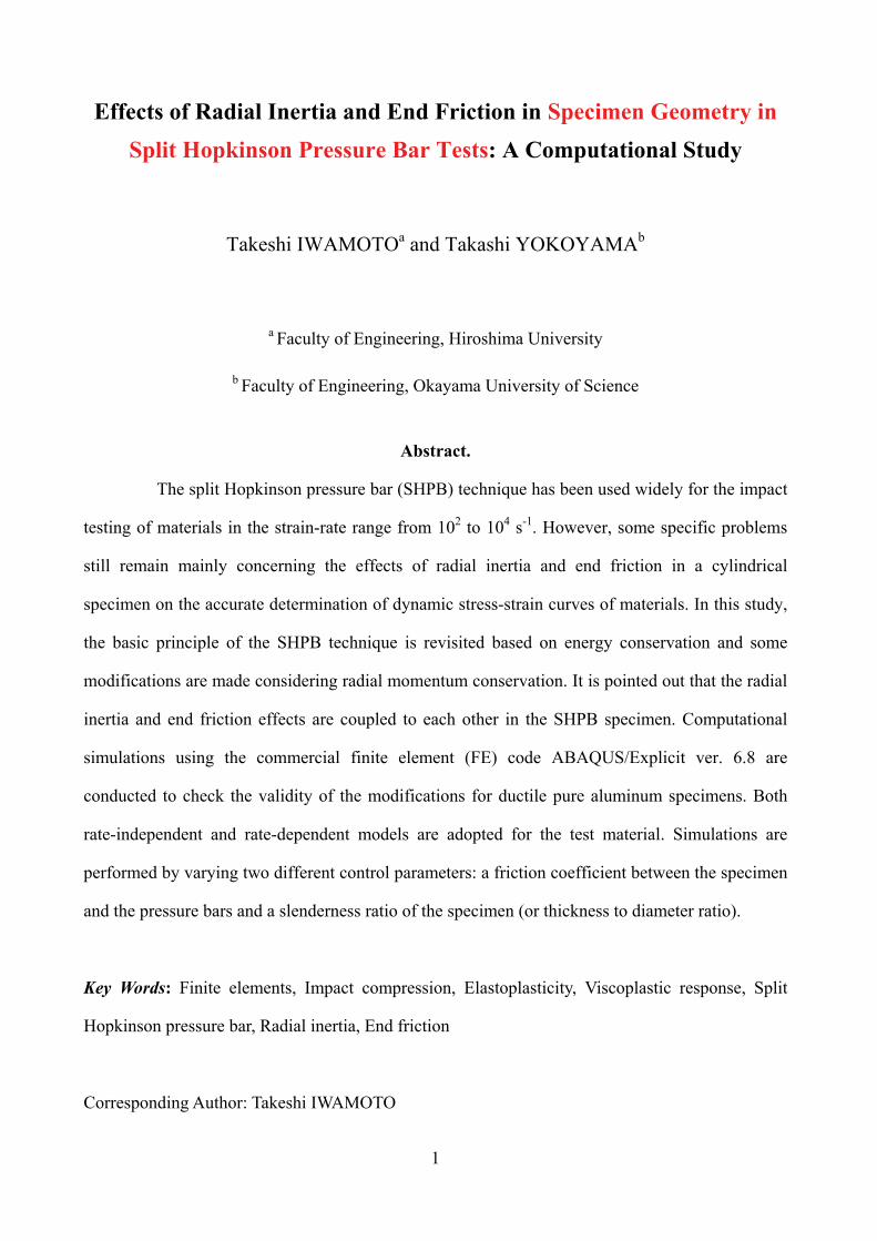
Effects of Radial Inertia and End Friction in Specimen Geometry in

Split Hopkinson Pressure Bar Tests: A Computational Study

Takeshi IWAMOTOa and Takashi YOKOYAMAb

a Faculty of Engineering, Hiroshima University

b Faculty of Engineering, Okayama University of Science

Abstract.

The split Hopkinson pressure bar (SHPB) technique has been used widely for the impact

testing of materials in the strain-rate range from 102 to 104 s-1. However, some specific problems

still remain mainly concerning the effects of radial inertia and end friction in a cylindrical

specimen on the accurate determination of dynamic stress-strain curves of materials. In this study,

the basic principle of the SHPB technique is revisited based on energy conservation and some

modifications are made considering radial momentum conservation. It is pointed out that the radial

inertia and end friction effects are coupled to each other in the SHPB specimen. Computational

simulations using the commercial finite element (FE) code ABAQUS/Explicit ver. 6.8 are

conducted to check the validity of the modifications for ductile pure aluminum specimens. Both

rate-independent and rate-dependent models are adopted for the test material. Simulations are

performed by varying two different control parameters: a friction coefficient between the specimen

and the pressure bars and a slenderness ratio of the specimen (or thickness to diameter ratio).

Key Words: Finite elements, Impact compression, Elastoplasticity, Viscoplastic response, Split

Hopkinson pressure bar, Radial inertia, End friction

Corresponding Author: Takeshi IWAMOTO

2

Postal address: Kagamiyama, Higashi-Hiroshima, Hiroshima, 739 - 8527 Japan

Tel: +81-82-424-7576, Fax.: +81-82-422-7193

E-mail: iwamoto@mec.hiroshima-u.ac.jp

3

1. INTRODUCTION

One of the most widely used test methods for determining dynamic stress-strain behavior of

materials is the split Hopkinson pressure bar (SHPB) technique originally developed by Kolsky

(1949). Before Kolsky (1949), two researchers (Taylor, 1946; Volterra, 1948) had the idea of using

pressure bars to measure the dynamic properties of materials in compression (Field et al., 2004). In

the experiments by Taylor (1946), a solid cylindrical specimen was fired against a massive and

rigid target. The dynamic flow stress of the specimen was estimated by measuring both lengths of

the deformed and the undeformed section of the specimen. Voltterra (1948) attempted to measure

the dynamic stress-strain curves of materials in this manner. A swinging impact pendulum was

used to directly strike a cylindrical specimen. In order to determine the specimen dynamic stress,

the acceleration was measured with an accelerometer placed on a uniform bar by which the

specimen was backed up.

In the conventional SHPB system, a short cylindrical specimen placed between two

elastic pressure bars is tested. Since its introduction, this technique has been applied in various

modes of loading, e.g., tension (Harding et al., 1960; Nicholas, 1981; Yokoyama, 2003), torsion

(Duffy et al., 1971), shear (Klepaczko, 1994; Rittel et al., 2002), three-point bending (Yokoyama

and Kishida, 1998), punching (Dowling et al., 1970; Dabboussi and Nemes, 2005), and used to

examine the dynamic response of hard materials such as ceramics (Klepaczko, 1990) and titanium

alloys (Khan et al., 2004; Khan et al., 2006; Khan et al., 2007), and soft materials such as rubbers

(Chen et al., 1999; Chen et al., 2002) and polymers (Khan and Zhang, 2001; Khan and Farrokh,

2006; Nakai and Yokoyama, 2008; Nishida et al., 2009; Farrokh and Khan, 2010; Khan et al.,

2010). However, some specific problems still remain regarding the effect of specimen size on end

friction and radial inertia. For more details, the reader can refer to several excellent reviews (Zhao

and Gary, 1996; Al-Mousawi et al., 1997; Zhao et al., 1997; Field et al., 2004; Gama et al., 2004).

Follansbee and Frantz (1983) discussed the effect of radial inertia on a one-dimensional elastic

wave propagation in a cylindrical bar, and pointed out that the radial inertia effect is coupled with

4

the axial acceleration. Many workers have difficulties in performing reliable impact tests at higher

impact velocities (> 20m/s) because the radial inertia effect becomes more significant. The end

friction and inertia effects are most critical, especially in the impact tests on brittle materials (Frew

et al., 2001; Frew et al., 2002). Several workers have a challenge to use the SHPB method with a

pulse shaper to overcome these complicated problems. (Frew et al., 2002; Chen et al., 2003)

Davies and Hunter (1963) first calculated the actual stress in a cylindrical specimen

using the law of energy conservation during impact testing. They discovered that there is a

difference between actual and measured stresses, which arises from radial inertia effects. In

addition, they found that a criterion for a specimen slenderness ratio = h / d (thickness h:

diameter d ratio) should be met for the specimen size to eliminate the difference. In recent years,

several attempts have been made to obtain compressive stress-stress data from the impact testing of

materials such as titanium alloys and stainless steels with higher strength than or equal to that of

the pressure bars. In such cases, it is needed to reduce the diameter as small as possible relative to

the diameter of the pressure bars to achieve reliable stress-strain data. This is why the specimen

with a smaller diameter than that of the pressure bars has usually been used. However, the diameter

of the specimen as well as that of the pressure bars should be determined to meet the assumptions

on the theory of one-dimensional elastic wave propagation, considering impedance mis-matching

between the specimen and the pressure bars. The effect of friction between the specimen and the

pressure bars should be investigated by separating them from the radial inertia effects. There is a

trade-off between the end friction and radial inertia effects.

The effects of end friction and radial inertia in the SHPB specimens have extensively

been studied using numerical simulations. Bertholf and Karnes (1975) presented a

two-dimensional numerical analysis of the governing wave equations for the SHPB using a finite

difference method. To find the optimum shape of the cylindrical specimen, Malinowski and

Klepaczko (1986) derived the equation that depends not only on the specimen diameter but also on

the stress, strain rate and time derivative of strain rate from the balance equation of the dissipation

energy consumed in friction. The validity of the optimum value obtained from the experiments and

5

numerical simulations was then assessed. Zencker and Clos (1999) simulated the compression

SHPB tests on the cylindrical specimen of a rate-dependent elastic-perfectly-plastic material using

the finite element method (FEM). They demonstrated that accurate dynamic stress-strain curves

can be obtained when the one-dimensional stress state lies in thin specimens with 0.5.

Similarly, accurate dynamic stress-strain data can be achieved if both the one-dimensional stress

state and uniformity of axial stress distribution are guaranteed in a relatively long specimen with

1. They found that the criterion for the optimum specimen slenderness ratio = 2/3

derived by Davies and Hunter (1963) does not seem to exist. Meng and Li (2003) also simulated

the compression SHPB tests on pure aluminum 1100 as the two-dimensional wave propagation

problem using the commercial FE code, and examined the effects of radial inertia and end friction.

In their simulations, rate-independent pure aluminum 1100 was used as the specimen material.

They showed that the stress in the specimen increases with increasing friction coefficient, and that

the optimum specimen slenderness ratio exists. Moreover, they pointed out that the correct

stress in the specimen cannot be determined if >1 under a frictionless condition between the

specimen and the pressure bars.

In the present study, the theory by Davies and Hunter (1963) is modified and the

relationship of radial inertia and friction between the specimen and the pressure bars is examined.

In addition, to verify the adequacy of the proposed theory based on the simulation results of Meng

and Li (2003), the compression SHPB tests on pure aluminum 1100 are simulated by the FEM. In

a series of simulations, two different control parameters are used: the slenderness ratio and the

friction coefficient . Two types of pure aluminum are considered as an example of ductile

metallic materials. A rate-independent material used by Meng and Li (2003) and a rate-dependent

material used by Bressan and Lopez (2008) are adopted as the test materials. The rate-independent

power-law strain hardening model for pure aluminum 1100 and the rate-dependent Johnson-Cook

model (Johnson and Cook, 1985) for another pure aluminum are introduced into the simulations to

assess the generality of the results obtained. The true stress can be evaluated directly from both

models with known constitutive parameters for the two types of pure aluminum (Meng and Li,

6

2003; Bressan and Lopez, 2008). The variations in the stress-strain curve with and are

examined by comparison with the FE results and direct calculations using both models. Note that

all the computations and energetic formulations are conducted within the framework of the

conventional continuum mechanics based on the Lagrangian coordinate, and hence any convection

terms are not be included. Even if the same topic is dealt with by Gorham (1989), the suitable

coordinate system should be chosen for both experiment and theory. Strain pulses were measured

by strain gauges glued on the pressure bars in the actual experiments. This implies that the strain

gauges are fixed on the material, not in a space. In this sense, the Lagrangian coordinate should be

chosen for the simulation if we attempt to compare with the experiments.

The structure of the paper is as follows. In Section 2, after a brief introduction of the

theory by Davies and Hunter (1963) including the formulation procedure, it will be shown that the

stress measured by the SHPB method does not depend on the specimen size, and that the nominal

strain rate during impact loading is kept constant by considering a radial momentum balance under

the frictionless condition to obtain accurate stress-strain responses. Then, the theory will be

extended by including the end friction effects into the radial momentum balance. The numerical

procedures using the commercial FE code will be described in Section 3. The computational model

of the SHPB test system along with the FE mesh division will be given. Computational conditions

including the two different control parameters and will be presented. Then, the results

computed by varying and are provided and some important discussions are given in

Section 4. The validity of the extended theory will be assessed. Finally, the results and discussion

will be summarized in Section 5.

2. BASIC THEORY

We derive energetic formulations again based on the Lagrangian coordinate. According to Davies

and Hunter (1963), we consider the specimen as shown in Fig. 1 with the cylindrical coordinate

system set at its center. The actual stress applied to the specimen, , can be expressed as

22

22

2 322

1a

hktcBB

, (1)

7

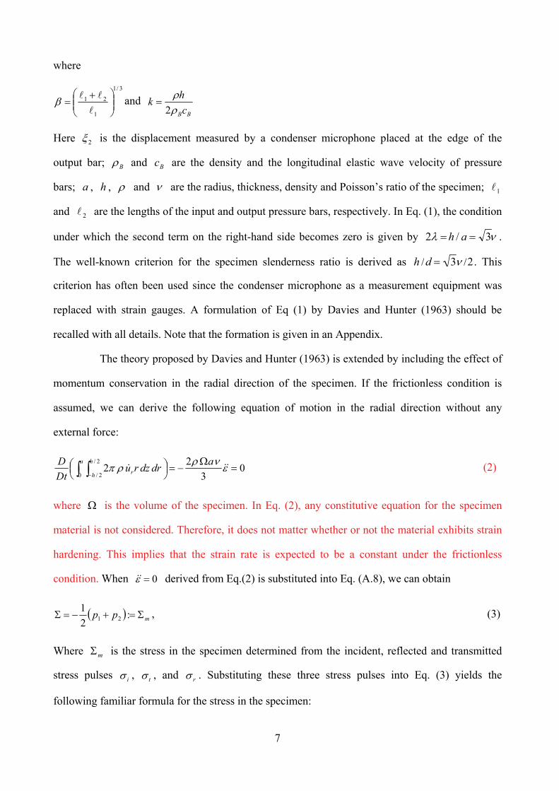
where

3/1

1

21

and BBc

hk

2

Here 2 is the displacement measured by a condenser microphone placed at the edge of the

output bar; B and Bc are the density and the longitudinal elastic wave velocity of pressure

bars; a , h , and are the radius, thickness, density and Poisson’s ratio of the specimen; 1

and 2 are the lengths of the input and output pressure bars, respectively. In Eq. (1), the condition

under which the second term on the right-hand side becomes zero is given by 3/2 ah .

The well-known criterion for the specimen slenderness ratio is derived as h /d 3 /2. This

criterion has often been used since the condenser microphone as a measurement equipment was

replaced with strain gauges. A formulation of Eq (1) by Davies and Hunter (1963) should be

recalled with all details. Note that the formation is given in an Appendix.

The theory proposed by Davies and Hunter (1963) is extended by including the effect of

momentum conservation in the radial direction of the specimen. If the frictionless condition is

assumed, we can derive the following equation of motion in the radial direction without any

external force:

03

22

0

2/

2/

adrdzru

Dt

D a h

h r (2)

where is the volume of the specimen. In Eq. (2), any constitutive equation for the specimen

material is not considered. Therefore, it does not matter whether or not the material exhibits strain

hardening. This implies that the strain rate is expected to be a constant under the frictionless

condition. When 0 derived from Eq.(2) is substituted into Eq. (A.8), we can obtain

mpp :2

121 , (3)

Where m is the stress in the specimen determined from the incident, reflected and transmitted

stress pulses i , t , and r . Substituting these three stress pulses into Eq. (3) yields the

following familiar formula for the stress in the specimen:

8

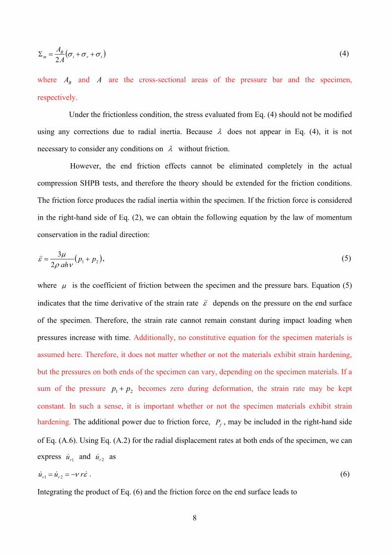
triB

m A

A 2

(4)

where BA and A are the cross-sectional areas of the pressure bar and the specimen,

respectively.

Under the frictionless condition, the stress evaluated from Eq. (4) should not be modified

using any corrections due to radial inertia. Because does not appear in Eq. (4), it is not

necessary to consider any conditions on without friction.

However, the end friction effects cannot be eliminated completely in the actual

compression SHPB tests, and therefore the theory should be extended for the friction conditions.

The friction force produces the radial inertia within the specimen. If the friction force is considered

in the right-hand side of Eq. (2), we can obtain the following equation by the law of momentum

conservation in the radial direction:

212

3pp

ah

, (5)

where is the coefficient of friction between the specimen and the pressure bars. Equation (5)

indicates that the time derivative of the strain rate depends on the pressure on the end surface

of the specimen. Therefore, the strain rate cannot remain constant during impact loading when

pressures increase with time. Additionally, no constitutive equation for the specimen materials is

assumed here. Therefore, it does not matter whether or not the materials exhibit strain hardening,

but the pressures on both ends of the specimen can vary, depending on the specimen materials. If a

sum of the pressure 21 pp becomes zero during deformation, the strain rate may be kept

constant. In such a sense, it is important whether or not the specimen materials exhibit strain

hardening. The additional power due to friction force, fP , may be included in the right-hand side

of Eq. (A.6). Using Eq. (A.2) for the radial displacement rates at both ends of the specimen, we can

express 1ru and 2ru as

ruu rr 21 . (6)

Integrating the product of Eq. (6) and the friction force on the end surface leads to

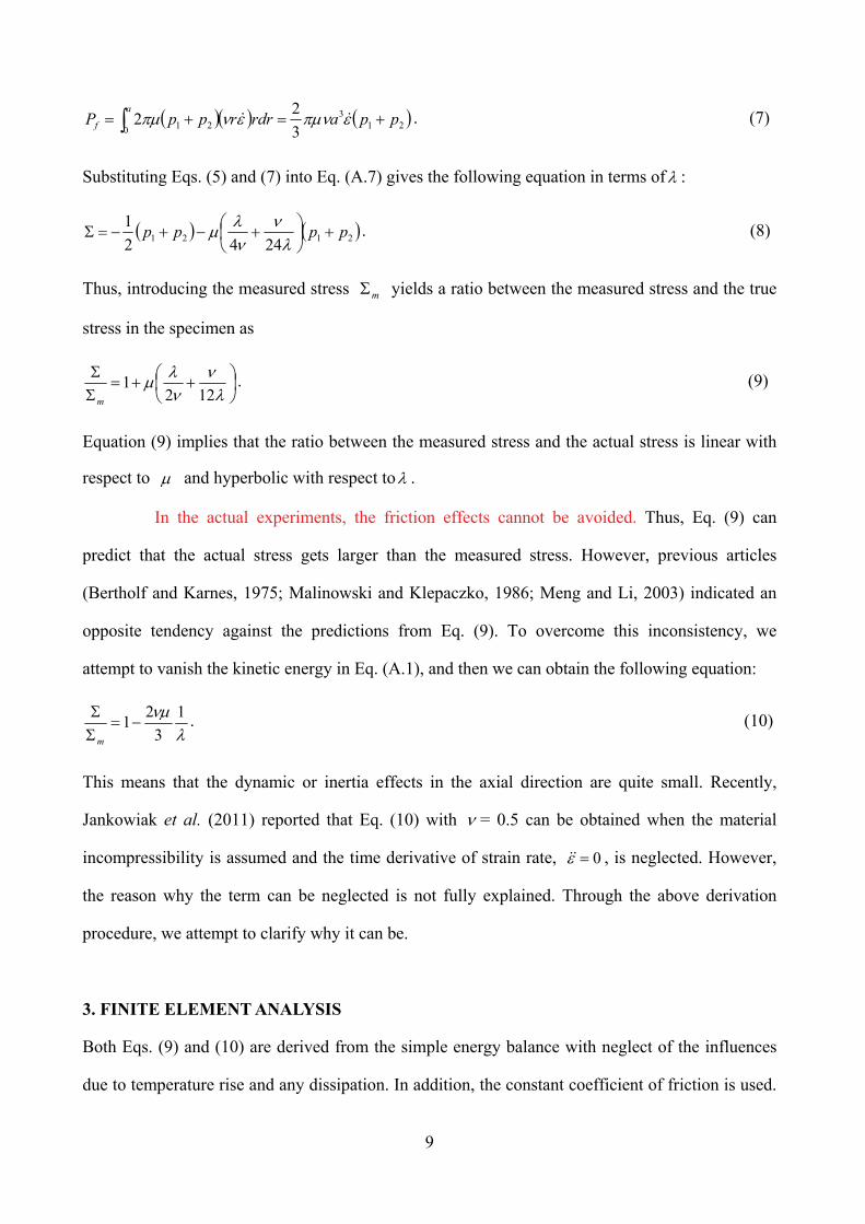
9

213

0 21 3

22 ppardrrppP

a

f . (7)

Substituting Eqs. (5) and (7) into Eq. (A.7) gives the following equation in terms of :

2121 2442

1pppp

. (8)

Thus, introducing the measured stress m yields a ratio between the measured stress and the true

stress in the specimen as

1221

m

. (9)

Equation (9) implies that the ratio between the measured stress and the actual stress is linear with

respect to and hyperbolic with respect to .

In the actual experiments, the friction effects cannot be avoided. Thus, Eq. (9) can

predict that the actual stress gets larger than the measured stress. However, previous articles

(Bertholf and Karnes, 1975; Malinowski and Klepaczko, 1986; Meng and Li, 2003) indicated an

opposite tendency against the predictions from Eq. (9). To overcome this inconsistency, we

attempt to vanish the kinetic energy in Eq. (A.1), and then we can obtain the following equation:

1

3

21

m

. (10)

This means that the dynamic or inertia effects in the axial direction are quite small. Recently,

Jankowiak et al. (2011) reported that Eq. (10) with = 0.5 can be obtained when the material

incompressibility is assumed and the time derivative of strain rate, 0 , is neglected. However,

the reason why the term can be neglected is not fully explained. Through the above derivation

procedure, we attempt to clarify why it can be.

3. FINITE ELEMENT ANALYSIS

Both Eqs. (9) and (10) are derived from the simple energy balance with neglect of the influences

due to temperature rise and any dissipation. In addition, the constant coefficient of friction is used.

10

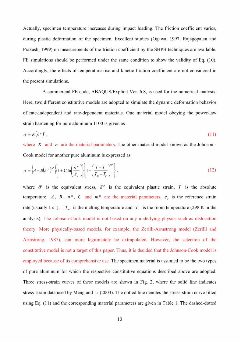
Actually, specimen temperature increases during impact loading. The friction coefficient varies,

during plastic deformation of the specimen. Excellent studies (Ogawa, 1997; Rajagopalan and

Prakash, 1999) on measurements of the friction coefficient by the SHPB techniques are available.

FE simulations should be performed under the same condition to show the validity of Eq. (10).

Accordingly, the effects of temperature rise and kinetic friction coefficient are not considered in

the present simulations.

A commercial FE code, ABAQUS/Explicit Ver. 6.8, is used for the numerical analysis.

Here, two different constitutive models are adopted to simulate the dynamic deformation behavior

of rate-independent and rate-dependent materials. One material model obeying the power-law

strain hardening for pure aluminum 1100 is given as

npK , (11)

where K and n are the material parameters. The other material model known as the Johnson -

Cook model for another pure aluminum is expressed as

*

0

*1ln1

m

rm

rp

np

TT

TTCBA

, (12)

where is the equivalent stress, p is the equivalent plastic strain, T is the absolute

temperature, A , B , *n , C and *m are the material parameters, 0 is the reference strain

rate (usually 1 s-1), mT is the melting temperature and rT is the room temperature (298 K in the

analysis). The Johnson-Cook model is not based on any underlying physics such as dislocation

theory. More physically-based models, for example, the Zerilli-Armstrong model (Zerilli and

Armstrong, 1987), can more legitimately be extrapolated. However, the selection of the

constitutive model is not a target of this paper. Thus, it is decided that the Johnson-Cook model is

employed because of its comprehensive use. The specimen material is assumed to be the two types

of pure aluminum for which the respective constitutive equations described above are adopted.

Three stress-strain curves of these models are shown in Fig. 2, where the solid line indicates

stress-strain data used by Meng and Li (2003). The dotted line denotes the stress-strain curve fitted

using Eq. (11) and the corresponding material parameters are given in Table 1. The dashed-dotted

11

line shows the stress-strain curve at a constant strain rate of 250 s-1 from the Johnson-Cook model,

whose constitutive parameters are identified by Bressan and Lopez (2008), and are listed in Table

2.

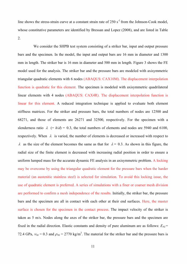
We consider the SHPB test system consisting of a striker bar, input and output pressure

bars and the specimen. In the model, the input and output bars are 16 mm in diameter and 1300

mm in length. The striker bar is 16 mm in diameter and 500 mm in length. Figure 3 shows the FE

model used for the analysis. The striker bar and the pressure bars are modeled with axisymmetric

triangular quadratic elements with 6 nodes (ABAQUS: CAX10M). The displacement interpolation

function is quadratic for this element. The specimen is modeled with axisymmetric quadrilateral

linear elements with 4 nodes (ABAQUS: CAX4R). The displacement interpolation function is

linear for this element. A reduced integration technique is applied to evaluate both element

stiffness matrices. For the striker and pressure bars, the total numbers of nodes are 12500 and

68271, and those of elements are 26271 and 32500, respectively. For the specimen with a

slenderness ratio (= h/d) = 0.3, the total numbers of elements and nodes are 5940 and 6100,

respectively. When is varied, the number of elements is decreased or increased with respect to

as the size of the element becomes the same as that for = 0.3. As shown in this figure, the

radial size of the finite element is decreased with increasing radial position in order to ensure a

uniform lumped mass for the accurate dynamic FE analysis in an axisymmetric problem. A locking

may be overcome by using the triangular quadratic element for the pressure bars when the harder

material (an austenitic stainless steel) is selected for simulation. To avoid this locking issue, the

use of quadratic element is preferred. A series of simulations with a finer or coarser mesh division

are performed to confirm a mesh independence of the results. Initially, the striker bar, the pressure

bars and the specimen are all in contact with each other at their end surfaces. Here, the master

surface is chosen for the specimen in the contact process. The impact velocity of the striker is

taken as 5 m/s. Nodes along the axes of the striker bar, the pressure bars and the specimen are

fixed in the radial direction. Elastic constants and density of pure aluminum are as follows: EAl =

72.4 GPa, Al = 0.3 and Al = 2770 kg/m3. The material for the striker bar and the pressure bars is

12

assumed to be a bearing steel with Young’s modulus BE = 208 GPa, Poisson’s ratio B = 0.3 and

density B = 7800 kg/m3. The kinematic contact pair algorithm is introduced at each contact

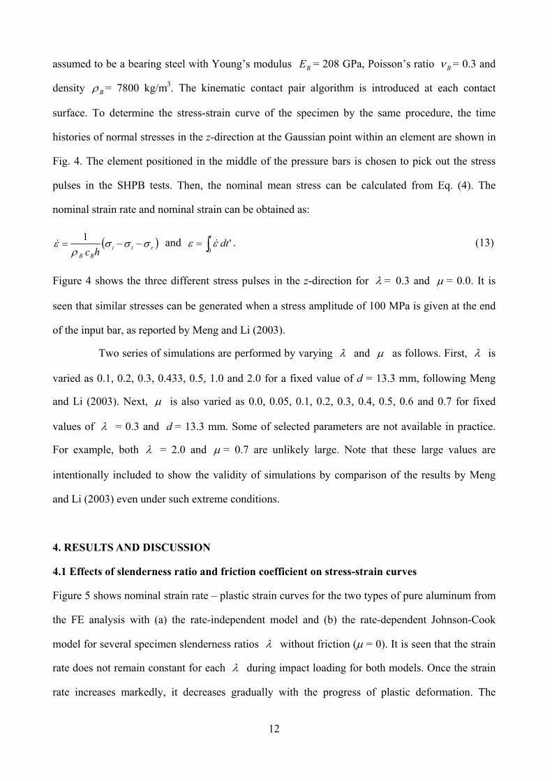
surface. To determine the stress-strain curve of the specimen by the same procedure, the time

histories of normal stresses in the z-direction at the Gaussian point within an element are shown in

Fig. 4. The element positioned in the middle of the pressure bars is chosen to pick out the stress

pulses in the SHPB tests. Then, the nominal mean stress can be calculated from Eq. (4). The

nominal strain rate and nominal strain can be obtained as:

rtiBB hc

1

and t

dt0

' . (13)

Figure 4 shows the three different stress pulses in the z-direction for = 0.3 and = 0.0. It is

seen that similar stresses can be generated when a stress amplitude of 100 MPa is given at the end

of the input bar, as reported by Meng and Li (2003).

Two series of simulations are performed by varying and as follows. First, is

varied as 0.1, 0.2, 0.3, 0.433, 0.5, 1.0 and 2.0 for a fixed value of d = 13.3 mm, following Meng

and Li (2003). Next, is also varied as 0.0, 0.05, 0.1, 0.2, 0.3, 0.4, 0.5, 0.6 and 0.7 for fixed

values of = 0.3 and d = 13.3 mm. Some of selected parameters are not available in practice.

For example, both = 2.0 and = 0.7 are unlikely large. Note that these large values are

intentionally included to show the validity of simulations by comparison of the results by Meng

and Li (2003) even under such extreme conditions.

4. RESULTS AND DISCUSSION

4.1 Effects of slenderness ratio and friction coefficient on stress-strain curves

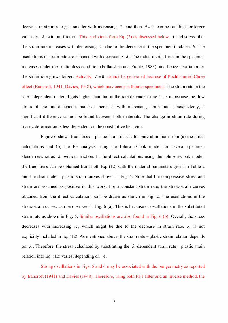
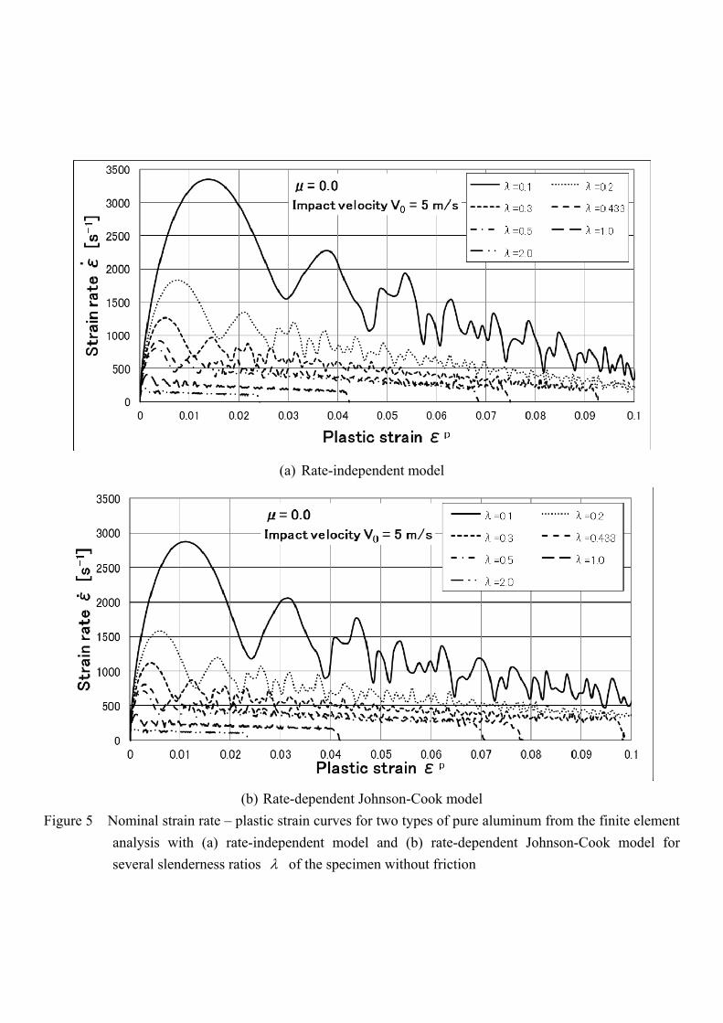
Figure 5 shows nominal strain rate – plastic strain curves for the two types of pure aluminum from

the FE analysis with (a) the rate-independent model and (b) the rate-dependent Johnson-Cook

model for several specimen slenderness ratios without friction ( = 0). It is seen that the strain

rate does not remain constant for each during impact loading for both models. Once the strain

rate increases markedly, it decreases gradually with the progress of plastic deformation. The

13

decrease in strain rate gets smaller with increasing , and then 0 can be satisfied for larger

values of without friction. This is obvious from Eq. (2) as discussed below. It is observed that

the strain rate increases with decreasing due to the decrease in the specimen thickness h. The

oscillations in strain rate are enhanced with decreasing . The radial inertia force in the specimen

increases under the frictionless condition (Follansbee and Frantz, 1983), and hence a variation of

the strain rate grows larger. Actually, 0 cannot be generated because of Pochhammer-Chree

effect (Bancroft, 1941; Davies, 1948), which may occur in thinner specimens. The strain rate in the

rate-independent material gets higher than that in the rate-dependent one. This is because the flow

stress of the rate-dependent material increases with increasing strain rate. Unexpectedly, a

significant difference cannot be found between both materials. The change in strain rate during

plastic deformation is less dependent on the constitutive behavior.

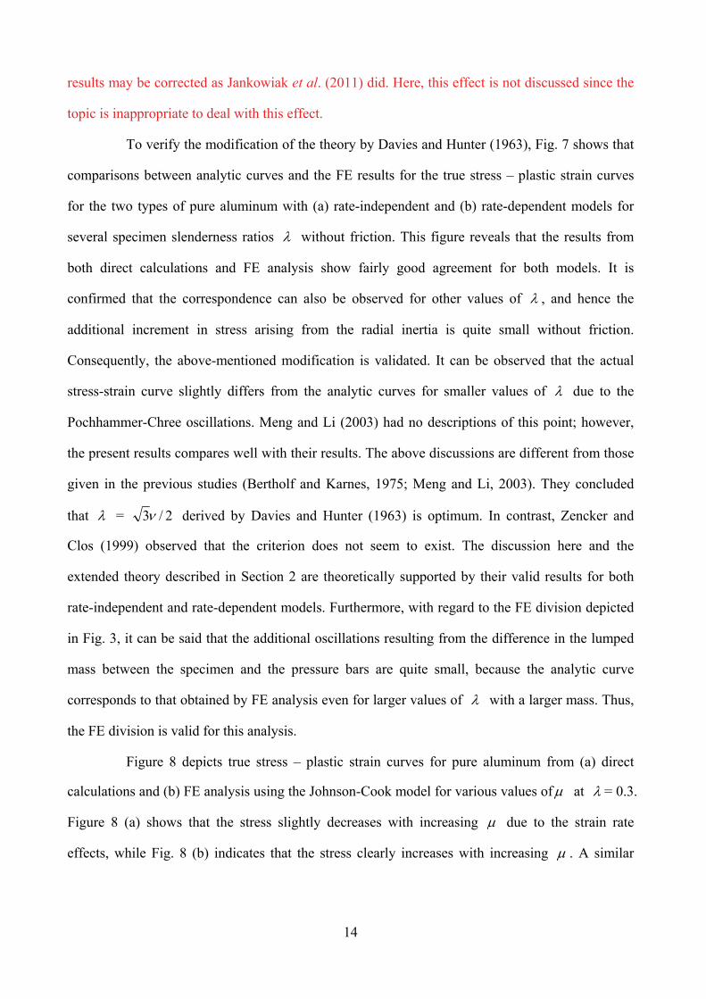
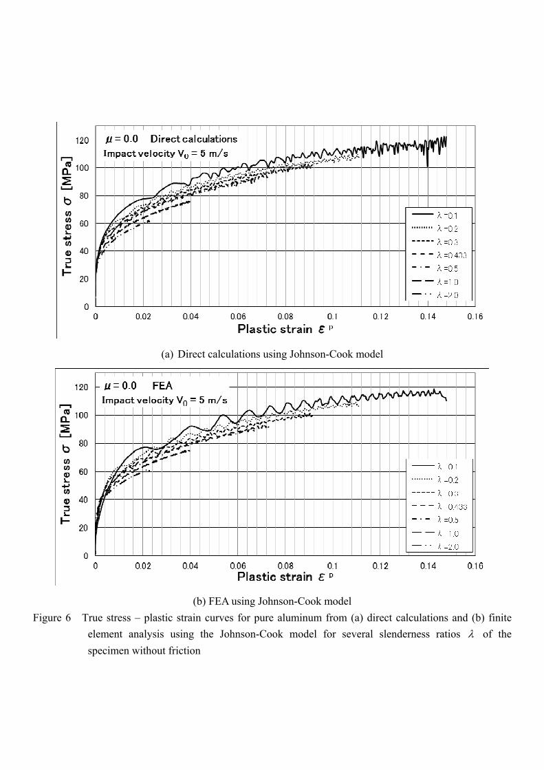
Figure 6 shows true stress – plastic strain curves for pure aluminum from (a) the direct

calculations and (b) the FE analysis using the Johnson-Cook model for several specimen

slenderness ratios without friction. In the direct calculations using the Johnson-Cook model,

the true stress can be obtained from both Eq. (12) with the material parameters given in Table 2

and the strain rate – plastic strain curves shown in Fig. 5. Note that the compressive stress and

strain are assumed as positive in this work. For a constant strain rate, the stress-strain curves

obtained from the direct calculations can be drawn as shown in Fig. 2. The oscillations in the

stress-strain curves can be observed in Fig. 6 (a). This is because of oscillations in the substituted

strain rate as shown in Fig. 5. Similar oscillations are also found in Fig. 6 (b). Overall, the stress

decreases with increasing , which might be due to the decrease in strain rate. is not

explicitly included in Eq. (12). As mentioned above, the strain rate – plastic strain relation depends

on . Therefore, the stress calculated by substituting the -dependent strain rate – plastic strain

relation into Eq. (12) varies, depending on .

Strong oscillations in Figs. 5 and 6 may be associated with the bar geometry as reported

by Bancroft (1941) and Davies (1948). Therefore, using both FFT filter and an inverse method, the

14

results may be corrected as Jankowiak et al. (2011) did. Here, this effect is not discussed since the

topic is inappropriate to deal with this effect.

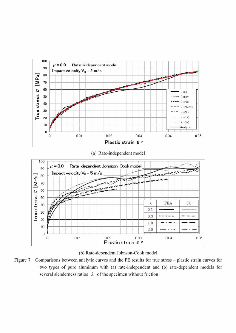
To verify the modification of the theory by Davies and Hunter (1963), Fig. 7 shows that

comparisons between analytic curves and the FE results for the true stress – plastic strain curves

for the two types of pure aluminum with (a) rate-independent and (b) rate-dependent models for

several specimen slenderness ratios without friction. This figure reveals that the results from

both direct calculations and FE analysis show fairly good agreement for both models. It is

confirmed that the correspondence can also be observed for other values of , and hence the

additional increment in stress arising from the radial inertia is quite small without friction.

Consequently, the above-mentioned modification is validated. It can be observed that the actual

stress-strain curve slightly differs from the analytic curves for smaller values of due to the

Pochhammer-Chree oscillations. Meng and Li (2003) had no descriptions of this point; however,

the present results compares well with their results. The above discussions are different from those

given in the previous studies (Bertholf and Karnes, 1975; Meng and Li, 2003). They concluded

that = 2/3 derived by Davies and Hunter (1963) is optimum. In contrast, Zencker and

Clos (1999) observed that the criterion does not seem to exist. The discussion here and the

extended theory described in Section 2 are theoretically supported by their valid results for both

rate-independent and rate-dependent models. Furthermore, with regard to the FE division depicted

in Fig. 3, it can be said that the additional oscillations resulting from the difference in the lumped

mass between the specimen and the pressure bars are quite small, because the analytic curve

corresponds to that obtained by FE analysis even for larger values of with a larger mass. Thus,

the FE division is valid for this analysis.

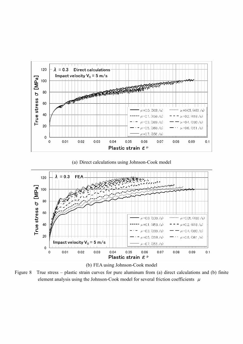
Figure 8 depicts true stress – plastic strain curves for pure aluminum from (a) direct

calculations and (b) FE analysis using the Johnson-Cook model for various values of at = 0.3.

Figure 8 (a) shows that the stress slightly decreases with increasing due to the strain rate

effects, while Fig. 8 (b) indicates that the stress clearly increases with increasing . A similar

15

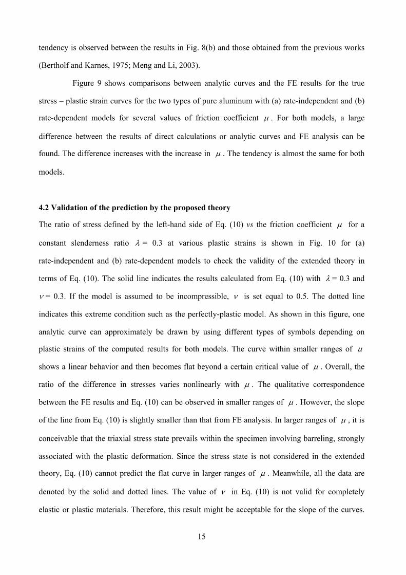
tendency is observed between the results in Fig. 8(b) and those obtained from the previous works

(Bertholf and Karnes, 1975; Meng and Li, 2003).

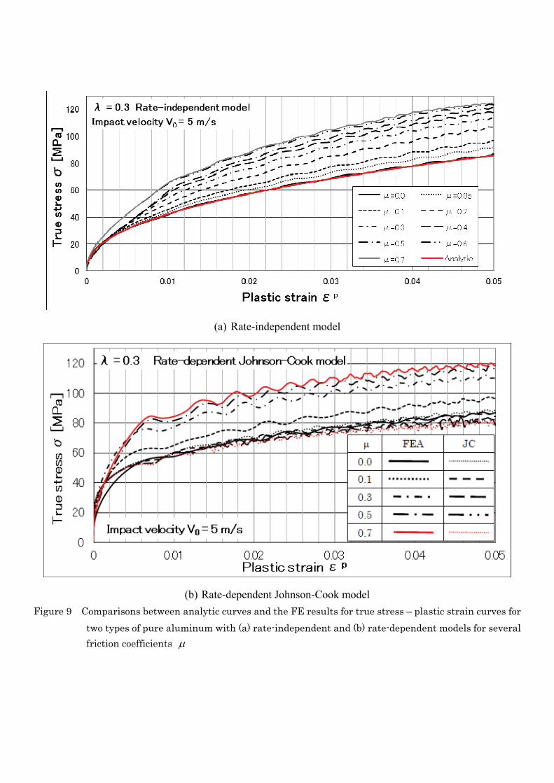
Figure 9 shows comparisons between analytic curves and the FE results for the true

stress – plastic strain curves for the two types of pure aluminum with (a) rate-independent and (b)

rate-dependent models for several values of friction coefficient . For both models, a large

difference between the results of direct calculations or analytic curves and FE analysis can be

found. The difference increases with the increase in . The tendency is almost the same for both

models.

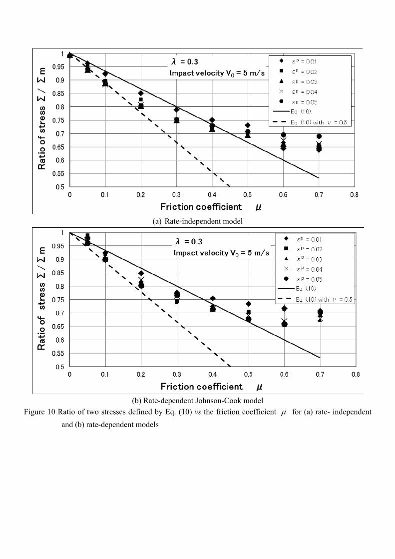
4.2 Validation of the prediction by the proposed theory

The ratio of stress defined by the left-hand side of Eq. (10) vs the friction coefficient for a

constant slenderness ratio = 0.3 at various plastic strains is shown in Fig. 10 for (a)

rate-independent and (b) rate-dependent models to check the validity of the extended theory in

terms of Eq. (10). The solid line indicates the results calculated from Eq. (10) with = 0.3 and

= 0.3. If the model is assumed to be incompressible, is set equal to 0.5. The dotted line

indicates this extreme condition such as the perfectly-plastic model. As shown in this figure, one

analytic curve can approximately be drawn by using different types of symbols depending on

plastic strains of the computed results for both models. The curve within smaller ranges of

shows a linear behavior and then becomes flat beyond a certain critical value of . Overall, the

ratio of the difference in stresses varies nonlinearly with . The qualitative correspondence

between the FE results and Eq. (10) can be observed in smaller ranges of . However, the slope

of the line from Eq. (10) is slightly smaller than that from FE analysis. In larger ranges of , it is

conceivable that the triaxial stress state prevails within the specimen involving barreling, strongly

associated with the plastic deformation. Since the stress state is not considered in the extended

theory, Eq. (10) cannot predict the flat curve in larger ranges of . Meanwhile, all the data are

denoted by the solid and dotted lines. The value of in Eq. (10) is not valid for completely

elastic or plastic materials. Therefore, this result might be acceptable for the slope of the curves.

16

As shown in this figure, these properties are independent of the types of materials. For OHFC

copper, Jankowiak et al. (2011) showed the similar curves on Fig. 10. The results obtained here are

quite consistent with their reliable data.

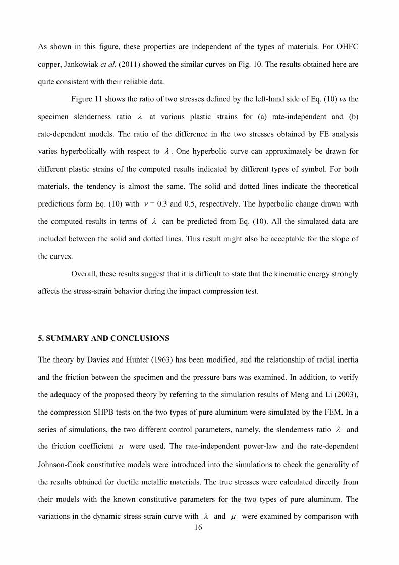
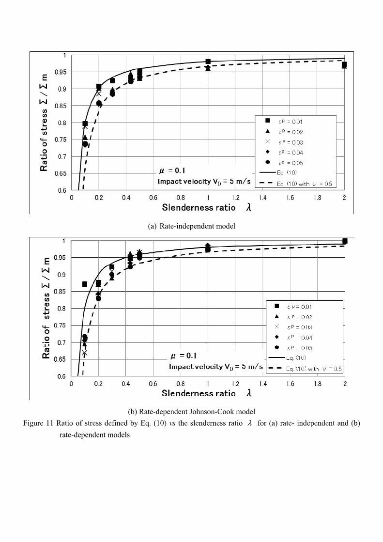
Figure 11 shows the ratio of two stresses defined by the left-hand side of Eq. (10) vs the

specimen slenderness ratio at various plastic strains for (a) rate-independent and (b)

rate-dependent models. The ratio of the difference in the two stresses obtained by FE analysis

varies hyperbolically with respect to . One hyperbolic curve can approximately be drawn for

different plastic strains of the computed results indicated by different types of symbol. For both

materials, the tendency is almost the same. The solid and dotted lines indicate the theoretical

predictions form Eq. (10) with = 0.3 and 0.5, respectively. The hyperbolic change drawn with

the computed results in terms of can be predicted from Eq. (10). All the simulated data are

included between the solid and dotted lines. This result might also be acceptable for the slope of

the curves.

Overall, these results suggest that it is difficult to state that the kinematic energy strongly

affects the stress-strain behavior during the impact compression test.

5. SUMMARY AND CONCLUSIONS

The theory by Davies and Hunter (1963) has been modified, and the relationship of radial inertia

and the friction between the specimen and the pressure bars was examined. In addition, to verify

the adequacy of the proposed theory by referring to the simulation results of Meng and Li (2003),

the compression SHPB tests on the two types of pure aluminum were simulated by the FEM. In a

series of simulations, the two different control parameters, namely, the slenderness ratio and

the friction coefficient were used. The rate-independent power-law and the rate-dependent

Johnson-Cook constitutive models were introduced into the simulations to check the generality of

the results obtained for ductile metallic materials. The true stresses were calculated directly from

their models with the known constitutive parameters for the two types of pure aluminum. The

variations in the dynamic stress-strain curve with and were examined by comparison with

17

the FE results and the direct calculations using their models. The main findings of the present

computational study are summarized as follows:

1) Under the frictionless conditions ( = 0), the accurate stress-strain behavior can be

characterized by the conventional SHPB method, and the strain rate can be constant during

impact loading. No corrections or reconstructions of the stress-strain curves are necessary.

However, large oscillations in the stress-strain curve appear when gets smaller. Any

suitable corrections should be taken into account.

2) The ratio between measured and analytic stress varies nonlinearly with according to the

proposed theory. Up to a certain value of , the curve shows a linear relationship. One curve

can approximately be drawn at different strains. The proposed theory can predict this linear

relationship.

3) The ratio between measured and analytic stress varies hyperbolically with respect to . Only

one curve can be plotted for any strains. However, the proposed theory can accurately predict

this relationship by neglecting the kinetic energy of the specimen.

18

Acknowledgement

The authors are grateful to Mr. Shiro YAMANAKA, graduate student of Hiroshima University, for

his assistance with finite element calculations. The ABAQUS program was provided under

academic license by Dassault Systèmes Simulia Corp., Providence, RI.

REFERENCES

Al-Mousawi, M. M., Reid, S. R., Deans, W. F., 1997. The use of the split Hopkinson pressure bar

techniques in high strain rate materials testing. Proc. Instn. Mech. Engrs. 211-Part C, 273 –

292.

Bancroft, D., 1941. The velocity of longitudinal waves in cylindrical bars. Phys. Rev. 59, 588 –

593.

Bertholf, L. D., Karnes, C. H., 1975. Two-dimensional analysis of the split Hopkinson pressure bar

system. J. Mech. Phys. Solids 23, 1 – 19.

Bressan, J. D., Lopez, K., 2008. New constitutive equation for plasticity in high speed torsion tests

of metals. Int. J. Mater. Form. Suppl. 1, 213 – 216.

Chen, W., Lu, F., Frew, D. J., Forrestal, M. J., 2002. Dynamic compression testing of soft

materials. Trans. ASME, J. Appl. Mech. 69, 214 – 223.

Chen, W., Song, B., Frew, D. J., Forrestal, M. J., 2003. Dynamic small strain measurements of a

metal specimen with a split Hopkinson pressure bar. Exp. Mech. 43, 20 – 23.

Chen, W., Zhang, B., Forrestal, M. J., 1999. A split Hopkinson bar technique for low-impedance

materials. Exp. Mech. 39, 81 – 85.

Dabboussi, W., Nemes, J. A., 2005. Modeling of ductile fracture using the dynamic punch test. Int.

J. Mech. Sci. 47, 1282 – 1299.

Davies, E. D. H., Hunter, S. C., 1963. The dynamic compression testing of solids by the method of

the split Hopkinson bar. J. Mech. Phys. Solids 11, 155 – 179.

19

Davies, R. M., 1948. A critical study of the split Hopkinson pressure bar. Philos. Trans. Roy. Soc.

London Ser. A 240, 375 – 457.

Dowling, A. R., Harding, J., Campbell, J. D., 1970. The dynamic punching of metals. J. Inst. Met.

98, 215 – 224.

Duffy, J., Campbell, J. D., Hawley, R. H., 1971. On the use of a torsional split Hopkinson bar to

study rate effects in 1100 0 aluminum. Trans. ASME, J. Appl. Mech. 38, 83 – 91.

Farrokh, B., Khan, A. S., 2010. A strain rate dependent yield criterion for isotropic polymers: Low

to high rates of loading. Eur. J. Mech. - A/Solids 29, 274 – 282.

Field, J. E., Walley, S. M., Proud, W. G., Goldrein, H. T., Siviour, C. R., 2004. Review of

experimental techniques for high rate deformation and shock studies. Int. J. Impact Engng. 30,

725 – 775.

Follansbee, P. S., Frantz, C., 1983. Wave propagation in the split Hopkinson pressure bar. Trans.

ASME, J. Engng. Mater. Technol. 105, 61 – 66.

Frew, D. J., Forrestal, M. J., Chen, W., 2001. A split Hopkinson pressure bar technique to

determine compressive stress-strain data for rock materials. Exp. Mech. 41, 40 – 46.

Frew, D. J., Forrestal, M. J., Chen, W., 2002. Pulse shaping techniques for testing brittle materials

with a split Hopkinson pressure bar. Exp. Mech. 42, 93 – 106.

Gama, B. A., Lopatnikov, S. L., Gillespie Jr, J. W., 2004. Hopkinson bar experimental technique: a

critical review. Appl. Mech. Rev., 57, 223 – 250.

Gorham, D.A., 1989, Specimen inertia in high strain-rate compression. J. Phys. D: Appl. Phys. 22,

1888 – 1893.

Harding, J., Wood, E. O., Campbell, J. D., 1960. Tensile testing of materials at impact rates of

strain. J. Mech. Eng. Sci. 2, 88 – 96.

20

Jankowiak, T., Rusinek, A., Lodygowski, T., 2011. Validation of the Klepaczko–Malinowski

model for friction correction and recommendations on split Hopkinson pressure bar. Fin. Elem.

Analy. Design. 47, 1191–1208

Johnson, G. R., Cook, W. H., 1985. Fracture characteristics of three metals subjected to various

strains, strain rates, temperatures and pressures. Engng. Fract. Mech. 21, 31–48.

Khan, A. S., Baig, M., Hamid, S., Zhang, H., 2010. Thermo-mechanical large deformation

responses of Hydrogenated Nitrile Butadiene Rubber (HNBR): Experimental results. Int. J.

Solids Struct. 47, 2653 – 2659.

Khan, A. S., Farrokh, B., 2006. Thermo-mechanical response of nylon 101 under uniaxial and

multi-axial loadings: Part I, Experimental results over wide ranges of temperatures and strain

rates. Int. J. Plast. 22, 1506 – 1529.

Khan, A. S., Kazmi, R., Farrokh, B., 2007. Multiaxial and non-proportional loading responses,

anisotropy and modeling of Ti–6Al–4V titanium alloy over wide ranges of strain rates and

temperatures. Int. J. Plast. 23, 931 – 950.

Khan, A. S., Kazmi, R., Farrokh, B., Zupan, M., 2006. Effect of oxygen content and microstructure

on the thermo-mechanical response of three Ti–6Al–4V alloys: Experiments and modeling

over a wide range of strain-rates and temperatures. Int. J. Plast. 23, 1105 – 1125.

Khan, A. S., Suh, Y. S., Kazmi, R., 2004. Quasi-static and dynamic loading responses and

constitutive modeling of titanium alloys. Int. J. Plast. 20, 2233 – 2248.

Khan, A. S., Zhang, H., 2001. Finite deformation of a polymer: experiments and modeling. Int. J.

Plast. 17, 1167 – 1188.

Klepaczko, J. R., 1990. Behavior of rock-like materials at high strain rates in compression. Int. J.

Plast. 6, 415 – 432.

Klepaczko, J. R., 1994. An experimental technique for shear testing at high and very high strain

rates: the case of a mild steel. Int. J. Impact Eng. 15, 25 – 39.

21

Kolsky, H., 1949. An investigation of the mechanical properties of materials at very high rates of

loading. Proc. Phys. Soc. B 62, 676 – 700.

Malinowski, J. Z., Klepaczko, J. R., 1986. A unified analytic and numerical approach to specimen

behaviour in the split-Hopkinson pressure bar. Int. J. Mech. Sci. 28, 381 – 391.

Meng, H., Li, Q. M., 2003. Correlation between the accuracy of a SHPB test and the stress

uniformity based on numerical experiments. Int. J. Impact Engng. 28, 537 – 555.

Nakai, K., Yokoyama, T., 2008. Strain rate dependence of compressive stress-strain loops of

several polymers. J. Solid Mech. Mater. Engng. 2, 557 – 566.

Nicholas, T., 1981. Tensile testing of materials at high rates of strain. Exp. Mech. 21, 177 – 185.

Nishida, M., Ito, N., Tanaka, K., 2009. Effects of strain rate and temperature on compressive

properties of a biodegradable resin made from oil. Zairyo, 58, 417 – 423. ( in Japanese )

Ogawa, K., 1997. Impact friction test method by applying stress wave. Exp. Mech. 37, 398 – 402.

Rajagopalan, S., Prakash, V., 1999. A modified torsional Kolsky bar for investigating dynamic

friction. Exp. Mech. 39, 295 – 303.

Rittel, D., Lee, S., Ravichandran, G., 2002. A shear-compression specimen for large strain testing.

Exp. Mech. 42, 58 – 64.

Taylor, G.I., 1946. The testing of materials at high rates of loading. J. Inst. Civil Engrs. 26, 486 –

519.

Volterra, E., 1948, Alcuni risultati di prove dinamiche sui materiali. Rivista Nuovo Cimento. 4, 1 –

28.

Yokoyama, T., 2003. Impact tensile stress-strain characteristics of wrought magnesium alloys.

Strain 39, 167 – 175.

Yokoyama, T., Kishida, K., 1989. A noble impact three-point bend test method for determining

dynamic fracture-initiation toughness. Exp. Mech. 29, 188 – 194.

22

Zerilli, F. J., Armstrong, R. W., 1987. Dislocation-mechanics-based constitutive relations for

material dynamics calculations. J. App. Phys. 61, 1816 – 1825.

Zencker, U., Clos, R., 1999. Limiting conditions for compression testing of flat specimens in the

split Hopkinson pressure bar. Exp. Mech. 39, 343 – 348.

Zhao, H., Gary, G., 1996. On the use of SHPB techniques to determine the dynamic behavior of

materials in the range of small strains. Int. J. Solid. Struct. 33, 3363 – 3375.

Zhao, H., Gary, G., Klepaczko, J. R., 1997. On the use of a viscoelastic split Hopkinson pressure

bar. Int. J. Impact Engng. 19, 319 – 330.

FIGURE CAPTIONS

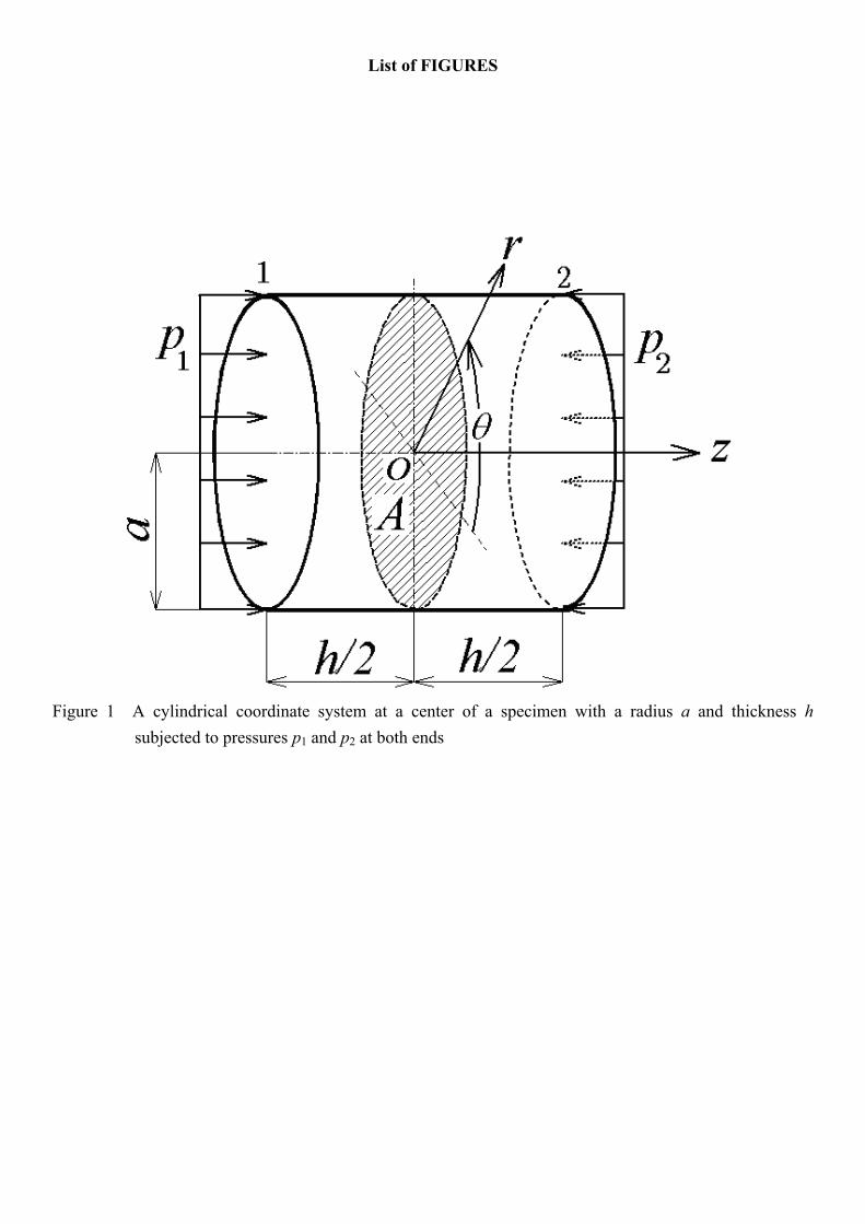
Figure 1 A cylindrical coordinate system at a center of a specimen with a radius a and thickness

h subjected to pressures p1 and p2 at both ends

Figure 2 Stress – strain curves for two types of pure aluminum with rate-independent model used

by Meng and Li (2003) and rate-dependent Johnson-Cook models used by Bressan and

Lopez (2008)

Figure 3 Finite element model of the split Hopkinson pressure bar test system

Figure 4 Example of three stress pulses on the input and output pressure bars from the finite

element calculations of the SHPB test on pure aluminum 1100

Figure 5 Nominal strain rate – plastic strain curves for two types of pure aluminum from the

finite element analysis with (a) rate-independent model and (b) rate-dependent

Johnson-Cook model for several slenderness ratios of the specimen without

friction

Figure 6 True stress – plastic strain curves for pure aluminum from (a) direct calculations and (b)

finite element analysis using the Johnson-Cook model for several slenderness ratios

of the specimen without friction

23

Figure 7 Comparisons between analytic curves and the FE results for true stress – plastic strain

curves for two types of pure aluminum with (a) rate-independent and (b)

rate-dependent models for several slenderness ratios of the specimen without

friction

Figure 8 True stress – plastic strain curves for pure aluminum from (a) direct calculations and (b)

finite element analysis using the Johnson-Cook model for several friction coefficients

Figure 9 Comparisons between analytic curves and the FE results for true stress – plastic strain

curves for two types of pure aluminum with (a) rate-independent and (b)

rate-dependent models for several friction coefficients

Figure 10 Ratio of two stresses defined by Eq. (10) vs the friction coefficient for (a) rate-

independent and (b) rate-dependent models

Figure 11 Ratio of stress defined by Eq. (10) vs the slenderness ratio for (a) rate- independent

and (b) rate-dependent models

TABLE CAPTIONS

Table 1 Material parameters of the rate-independent power-law strain hardening model for pure

aluminum 1100 used by Meng and Li (2003)

Table 2 Material parameters of the rate-dependent Johnson-Cook model for pure aluminum used

by Bressan and Lopez (2008)

24

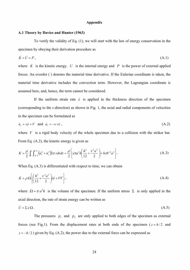
Appendix

A.1 Theory by Davies and Hunter (1963)

To verify the validity of Eq. (1), we will start with the law of energy conservation in the

specimen by obeying their derivation procedure as

PUK , (A.1)

where K is the kinetic energy, U is the internal energy and P is the power of external applied

forces. An overdot (•) denotes the material time derivative. If the Eulerian coordinate is taken, the

material time derivative includes the convection term. However, the Lagrangian coordinate is

assumed here, and, hence, the term cannot be considered.

If the uniform strain rate is applied in the thickness direction of the specimen

(corresponding to the z-direction) as shown in Fig. 1, the axial and radial components of velocities

in the specimen can be formulated as

Vzuz and rur , (A.2)

where V is a rigid body velocity of the whole specimen due to a collision with the striker bar.

From Eq. (A.2), the kinetic energy is given as

22222

2

0

2/

2/

22

21222

2aVh

ahhardrdzuuK

a h

h zr . (A.3)

When Eq. (A.3) is differentiated with respect to time, we can obtain

VV

ahK

212

222

, (A.4)

where ha2 is the volume of the specimen. If the uniform stress is only applied in the

axial direction, the rate of strain energy can be written as

U . (A.5)

The pressures 1p and 2p are only applied to both edges of the specimen as external

forces (see Fig.1). From the displacement rates at both ends of the specimen ( 2/hz and

2/hz ) given by Eq. (A.2), the power due to the external force can be expressed as

25

212121 222pp

AhVppAV

hApV

hApP

. (A.6)

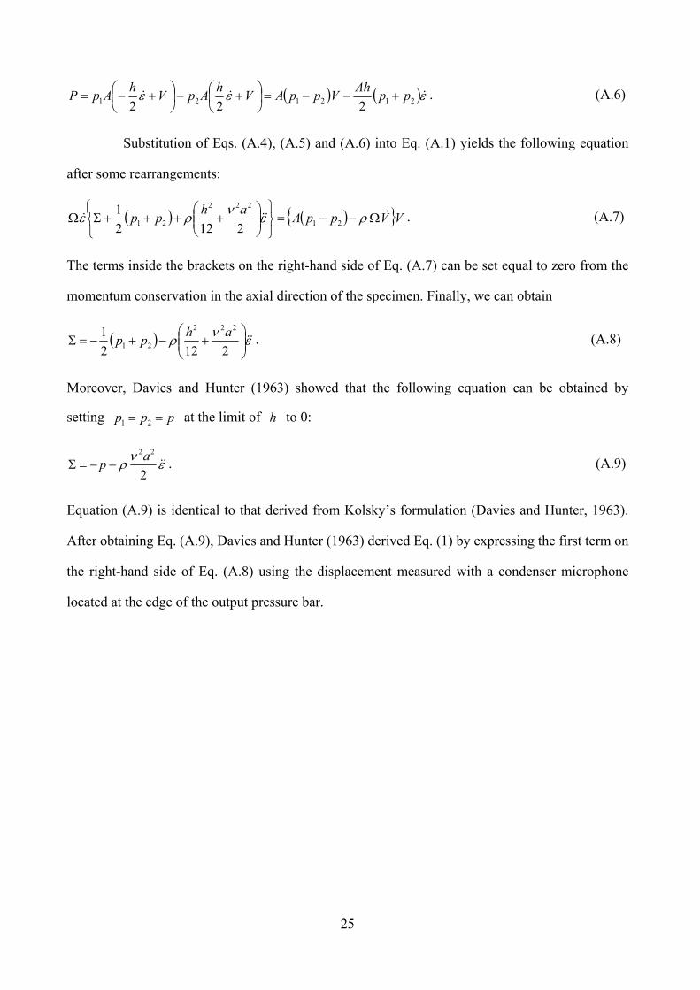
Substitution of Eqs. (A.4), (A.5) and (A.6) into Eq. (A.1) yields the following equation

after some rearrangements:

VVppAah

pp

21

222

21 2122

1 . (A.7)

The terms inside the brackets on the right-hand side of Eq. (A.7) can be set equal to zero from the

momentum conservation in the axial direction of the specimen. Finally, we can obtain

2122

1 222

21

ahpp . (A.8)

Moreover, Davies and Hunter (1963) showed that the following equation can be obtained by

setting ppp 21 at the limit of h to 0:

2

22ap . (A.9)

Equation (A.9) is identical to that derived from Kolsky’s formulation (Davies and Hunter, 1963).

After obtaining Eq. (A.9), Davies and Hunter (1963) derived Eq. (1) by expressing the first term on

the right-hand side of Eq. (A.8) using the displacement measured with a condenser microphone

located at the edge of the output pressure bar.

List of FIGURES

Figure 1 A cylindrical coordinate system at a center of a specimen with a radius a and thickness h

subjected to pressures p1 and p2 at both ends

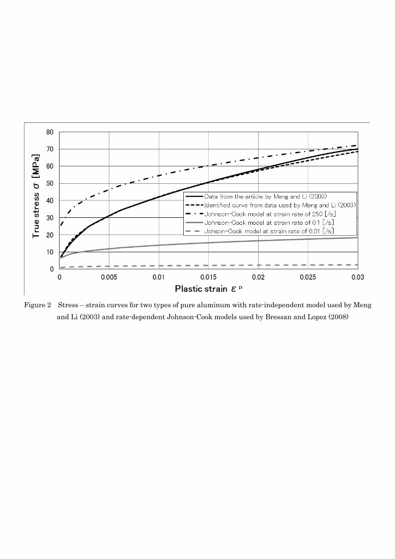
Figure 2 Stress – strain curves for two types of pure aluminum with rate-independent model used by Meng

and Li (2003) and rate-dependent Johnson-Cook models used by Bressan and Lopez (2008)

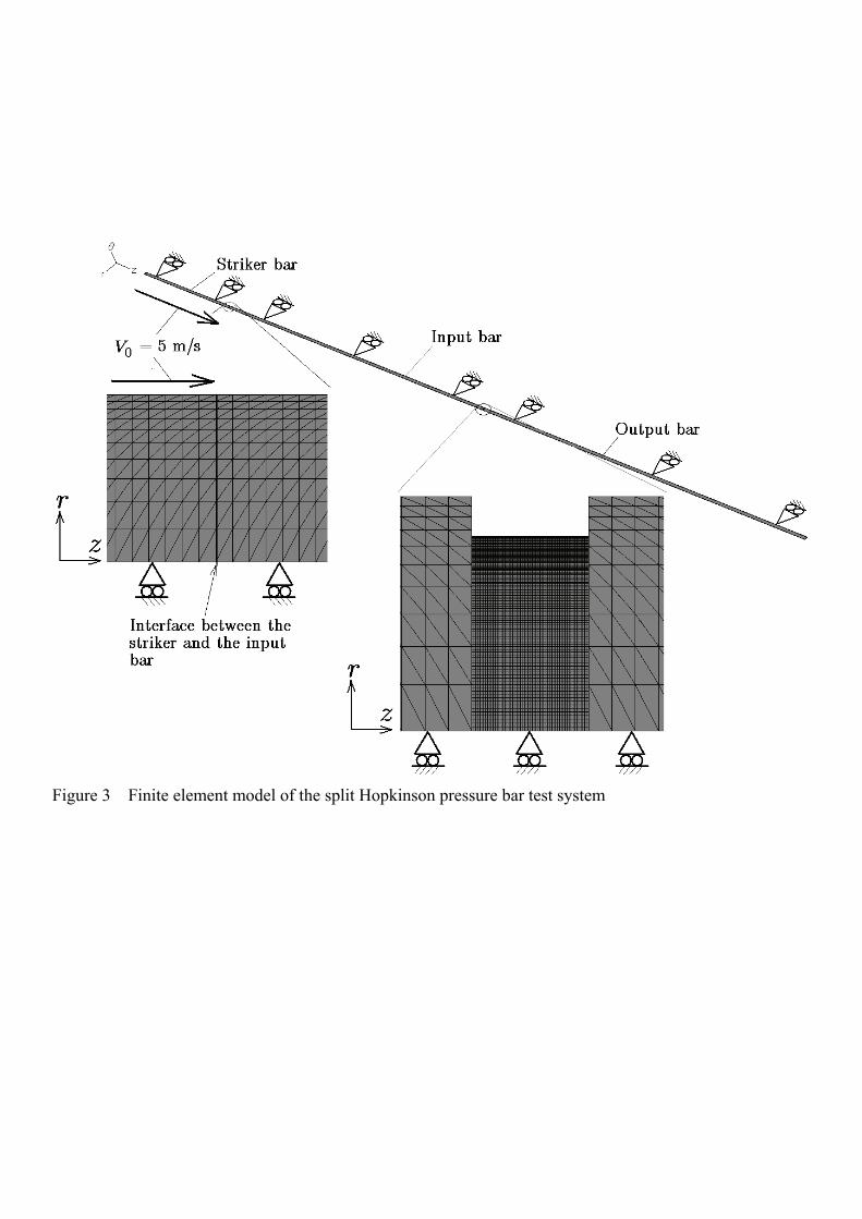
Figure 3 Finite element model of the split Hopkinson pressure bar test system

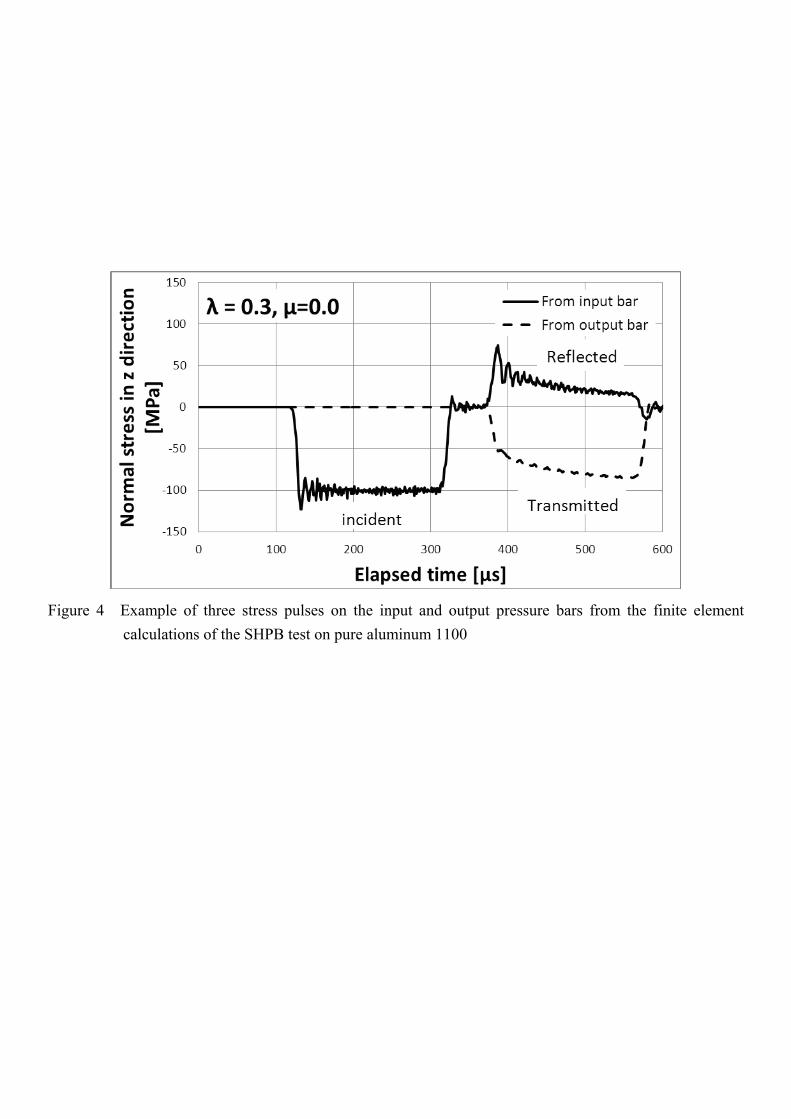
Figure 4 Example of three stress pulses on the input and output pressure bars from the finite element

calculations of the SHPB test on pure aluminum 1100

(a) Rate-independent model

(b) Rate-dependent Johnson-Cook model

Figure 5 Nominal strain rate – plastic strain curves for two types of pure aluminum from the finite element

analysis with (a) rate-independent model and (b) rate-dependent Johnson-Cook model for

several slenderness ratios of the specimen without friction

(a) Direct calculations using Johnson-Cook model

(b) FEA using Johnson-Cook model

Figure 6 True stress – plastic strain curves for pure aluminum from (a) direct calculations and (b) finite

element analysis using the Johnson-Cook model for several slenderness ratios of the

specimen without friction

(a) Rate-independent model

(b) Rate-dependent Johnson-Cook model

Figure 7 Comparisons between analytic curves and the FE results for true stress – plastic strain curves for

two types of pure aluminum with (a) rate-independent and (b) rate-dependent models for

several slenderness ratios of the specimen without friction

(a) Direct calculations using Johnson-Cook model

(b) FEA using Johnson-Cook model

Figure 8 True stress – plastic strain curves for pure aluminum from (a) direct calculations and (b) finite

element analysis using the Johnson-Cook model for several friction coefficients

(a) Rate-independent model

(b) Rate-dependent Johnson-Cook model

Figure 9 Comparisons between analytic curves and the FE results for true stress – plastic strain curves for

two types of pure aluminum with (a) rate-independent and (b) rate-dependent models for several

friction coefficients

(a) Rate-independent model

(b) Rate-dependent Johnson-Cook model

Figure 10 Ratio of two stresses defined by Eq. (10) vs the friction coefficient for (a) rate- independent

and (b) rate-dependent models

(a) Rate-independent model

(b) Rate-dependent Johnson-Cook model

Figure 11 Ratio of stress defined by Eq. (10) vs the slenderness ratio for (a) rate- independent and (b)

rate-dependent models

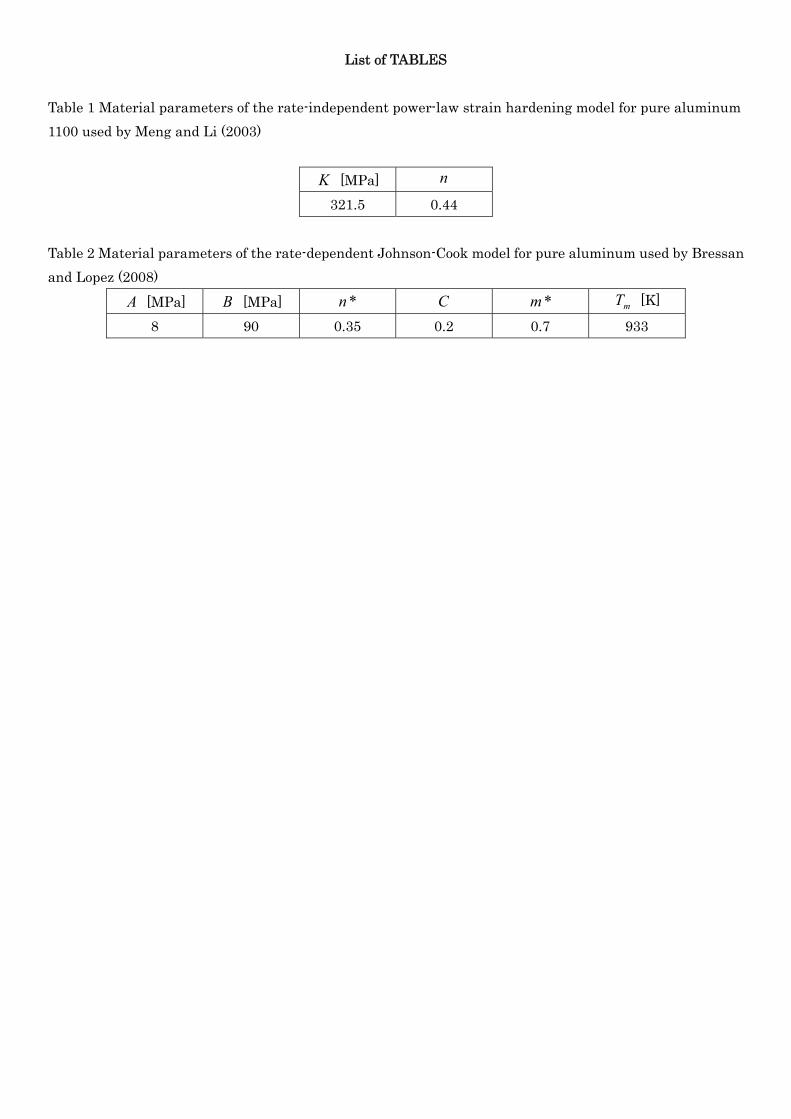
List of TABLES

Table 1 Material parameters of the rate-independent power-law strain hardening model for pure aluminum

1100 used by Meng and Li (2003)

K [MPa] n

321.5 0.44

Table 2 Material parameters of the rate-dependent Johnson-Cook model for pure aluminum used by Bressan

and Lopez (2008)

A [MPa] B [MPa] *n C *m mT [K]

8 90 0.35 0.2 0.7 933