I529: Machine Learning in Bioinformatics (Spring 2013)

HMM: Parameter Estimation

Yuzhen Ye School of Informatics and Computing

Indiana University, Bloomington Spring 2013

Content   Review

–  HMM: three problems –  The forward & backward algorithms; will be used

again for the training of HMM   When the training sequences are annotated

(with known states)—MLE estimations   When the states are unknown—Baum Welch

training –  An EM algorithm –  E step—calculate Akl and Ek(b) –  M step

Parameters defining a HMM

A Markov chain over a set of (hidden) states, and for each state s and observable symbol x, an emission probability p(Xi=x|Si=s).

HMM consists of:

An HMM model is defined by the parameters: akl (transition probabilities) and ek(b) (emission probabilities), for all states k,l and all symbols b. Let θ denote the collection of these parameters.

l k

b

akl

ek(b)

Parameter estimation for HMM

To determine the values of (the parameters in) θ, use a training set = {x1,...,xn}, where each xj is a sequence which is assumed to fit the model. Given the parameters θ, each sequence xj has an assigned probability p(xj|θ).

s1 s2 sL-1 sL

X1 X2 XL-1 XL

si

Xi

Data for HMM learning

Properties of (the sequences in) the training set: 1. For each xj, the information on the states sj

i The input sequences are annotated by the

corresponding hidden sequences. 2. The size (number of sequences) of the training set

To determine the values of (the parameters in) θ, use a training set = {x1,...,xn}, where each xj is a sequence which is assumed to fit the model. Given the parameters θ, each sequence xj has an assigned probability p(xj|θ).

Maximum likelihood parameter estimation for HMM The elements of the training set {x1,...,xn}, are assumed to be independent, p(x1,..., xn|θ) = ∏j p (xj|θ). ML parameter estimation looks for θ which maximizes the above. The exact method for finding or approximating this θ depends on the nature of the training set used.

Case 1: State paths are fully known

The training set {x1,...,xn}

By the ML method, we look for parameters θ* (akl and ek(b)) which maximize the probability of the sample set: p(x1,...,xn| θ*) =MAXθ p(x1,...,xn| θ).

s1 s2 sL-1 sL

X1 X2 XL-1 XL

si

Xi

Case 1: State paths are fully known

p (x j |θ ) = aklmkl

(k ,l )∏ [ek (b)]

mk (b )

(k ,b )∏

mkl= #(transitions from k to l) in sequence xj . mk(b)=#(emissions of symbol b from state k) in sequence xj .

For a sequence xj : ∏=

−=

L

i

jisss

j xeaxpiii

1

)()|(1

θ

For the entire training set: Akl = #(transitions from k to l) in the training set. Ek(b) = #(emissions of symbol b from state k) in the training set.

aklAkl

(k ,l )∏ [ek (b)]

Ek (b )

(k ,b )∏

k Subject to: for all states , 1, and e ( ) 1, , ( ) 0.kl kl kl b

k a b a e b= = ≥∑ ∑

We need to maximize:

MLE for n outcomes

The MLE is given by the relative frequencies:

1,..,iini k

nθ = =

MLE applied to HMM

'' '

( ) , and ( )( ')

kl kkl k

kl kl b

A E ba e bA E b

= =∑ ∑

We apply the previous technique to get for each k the parameters {akl|l=1,..,m} and {ek(b)|b∈Σ}:

Which gives the optimal ML parameters

Adding pseudo counts in HMM

' '' '

( ) ( )then , and ( )( ) ( ( ') ( ))kl kl k k

kl kkl kl k kl b

A r E b r ba e bA r E b r b+ +

= =+ +∑ ∑

If the sample set is too small, we may get a biased result. In this case we modify the actual count by our prior knowledge/belief: rkl is our prior belief and transitions from k to l. rk(b) is our prior belief on emissions of b from state k.

Fair casino problem: the sequences are annotated   Consider the fair casino, where the dealer may use two coins

(First and Second).   HMM: the hidden states are {F(air), B(iased)}, observation

symbols are {H(head), T(ail)}. We want to approximate the HMM parameters, the initial probabilities a0F and a0B, the transition probabilities aFF, aFB, aBF, and aBB, the emission probabilities eF(T), eF(H), eB(T) and eS(H).

  When the training set contains annotated sequences, we can simply compute the frequency for each of these cases to estimate the corresponding probabilities, which proved to be the Maximum Likelihood model parameters.

Fair casino problem: learning Training sequences Seq1 Seq2

Obs: TTHTHHTTHH Obs: THHTHHHHHHTTHH

Hid: FFFFBBBBBB Hid: FFFFFBBBBBFFFF

MLE a0F=#F/2=1.0, a0B=#B/2=0.0 aFF = #(FF)/#(Fx) = 10/12 = 0.83; aFB = #(FB)/#(Fx)=2/12=0.17 aBF = #(BF)/#(Bx) = 1/10=0.1; aBB = #(BB)/#(Bx)= 9/10=0.9 Fx means the di-hidden states with F as the first state. eF(T) = #(T,F)/#(F)= 7/13=0.53; eF(H)= #(H,F)/#(F)=6/13=0.47 eB(T) = #(T,B)/#(B) = 2/11=0.18; eB(H) = #(H,B)/#(B)=9/11=0.82

Case 2: State paths are unknown

For a given θ we have: p(x1,..., xn|θ)= p(x1| θ) ⋅ ⋅ ⋅ p (xn|θ)

(since the xj are independent)

s1 s2 sL-1 sL

X1 X2 XL-1 XL

si

Xi

For each sequence x: p(x|θ)=∑s p(x,s|θ) The sum taken over all hidden state paths s!

Finding θ* which maximizes ∑s p(x,s|θ) is hard.

The general process for finding θ in this case is 1.  Start with an initial value of θ. 2.  Find θ’ so that p(x|θ’) > p(x|θ) 3.  set θ = θ’. 4.  Repeat until some convergence criterion is met.

A general algorithm of this type is the Expectation Maximization algorithm, which we will meet later. For the specific case of HMM, it is the Baum-Welch training.

ML Parameter Estimation for HMM

Baum Welch training

We start with some values of akl and ek(b), which define prior values of θ. Then we use an iterative algorithm which attempts to replace θ by a θ* s.t.

p(x|θ*) > p(x|θ) This is done by “imitating” the algorithm for Case 1, where all states are known:

s1 s2 sL-1 sL

X1 X2 XL-1 XL

si

Xi

Baum Welch training

When the states are known, we can simply count. However, when the states are unknown, the “counting” process is a little trickier; instead, we use averaging process. For each edge si-1 si we compute the average number of “k to l” transitions, for all possible pairs (k,l), over this edge. Then, for each k and l, we take Akl to be the sum over all edges.

Si= ? Si-1= ?

xi-1= b xi= c

… …

Computing P(si-1=k, si=l | x,θ)

P(x1,…,xL,si-1=k,si=l|θ) = P(x1,…,xi-1,si-1=k|θ) aklel(xi ) P(xi+1,…,xL |si=l,θ) = fk(i-1) aklel(xi ) bl(i)

s1 s2 sL-1 sL

X1 X2 XL-1 XL

Si-1

Xi-1

si

Xi

x

p(si-1=k,si=l | x,θ ) = fk(i-1) aklel(xi ) bl(i) )|( θxp

Compute Akl for one sequence For each pair (k,l), compute the expected number of state transitions from k to l, as the sum of the expected number of k to l transitions over all L edges :

Akl =1

p (x |θ )p (si −1 = k , si = l , x |θ )

i =1

L

∑

Akl =1

p (x |θ )f k (i −1)akl el

i =1

L

∑ (xi )bl (i )

Compute Akl for many sequences

Akl =1

p (x j )j =1

n

∑ p (si −1=k ,si =l ,x j |θ )i =1

L

∑

Akl =1

p (x j )j =1

n

∑ f kj (i −1)akl el (xi )bl

j (i )i =1

L

∑

When we have n independent input sequences (x1,..., xn ), then Akl is given by:

where and are the forward and backward algorithms

for under .

j jk lf bjx θ

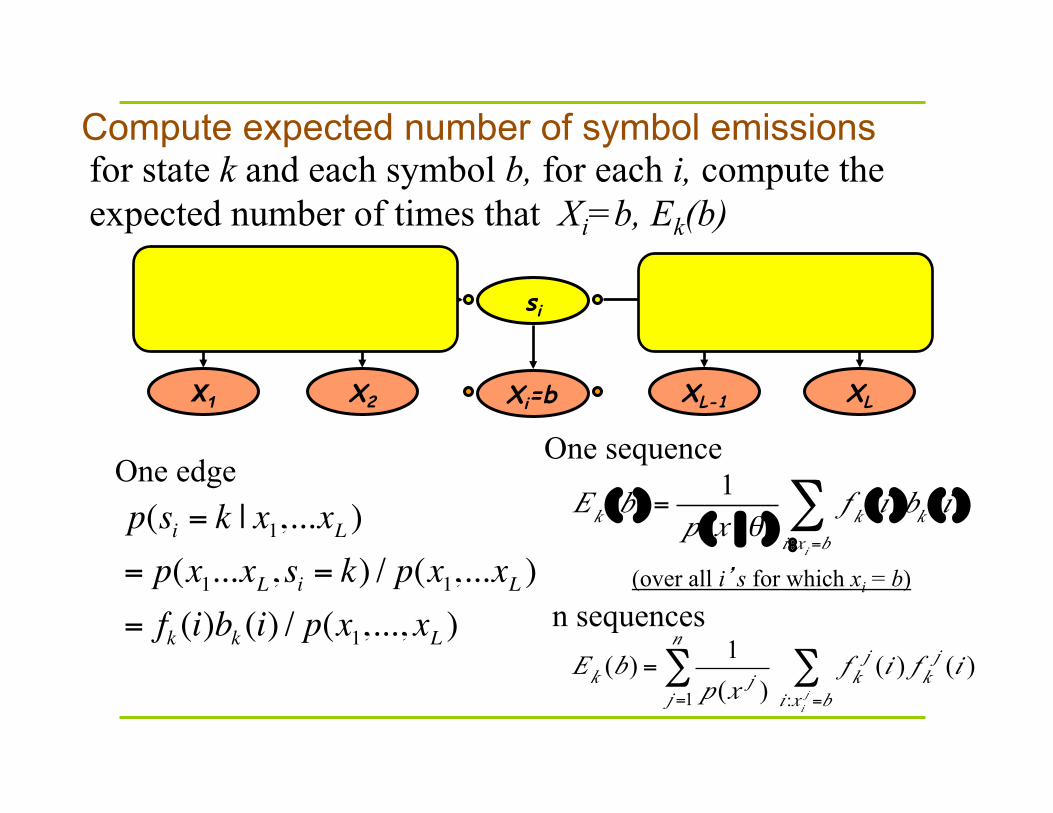
Compute expected number of symbol emissions

Ek (b) = 1p (x j )j =1

n

∑ f kj (i ) f k

j (i )i :xi

j =b∑

for state k and each symbol b, for each i, compute the expected number of times that Xi=b, Ek(b)

s1 s2 sL-1 sL

X1 X2 XL-1 XL

si

Xi=b

p(si = k | x1,...xL )= p(x1...xL, si = k) / p(x1,...xL )= fk (i)bk (i) / p(x1,..., xL )

Ek (b ) =1

p (x |θ )f k (i )bk (i )

i :xi =b∑

(over all i’s for which xi = b)

One edge One sequence

n sequences

Summary of the E step

Task: compute the expected numbers Akl of k,l transitions for all pairs of states k and l, and the expected numbers Ek(b) of transmisions of symbol b from state k, for all states k and symbols b. The next step is the M step, which is identical to the computation of optimal ML parameters when all states are known.

Baum Welch: M step

'' '

( ) , and ( )( ')

kl kkl k

kl kl b

A E ba e bA E b

= =∑ ∑

Use the Akl’s, Ek(b)’s to compute the new values of akl and ek(b). These values define θ*.

The correctness of the EM algorithm implies that: p(x1,..., xn|θ*) ≥ p(x1,..., xn|θ)

i.e, θ* increases the probability of the data This procedure is iterated, until some convergence criterion is met. Be aware of the local maximum (minimum) problem!