Chapter 56: Hydroplaning Simulation

56 Hydroplaning Simulation

Summary 1114

Introduction 1115

Requested Solution 1115

Modeling Details 1115

Results 1116

Postprocessing with SimXpert 1119

Input File(s) 1129

Video 1130

MD Demonstration Problems

CHAPTER 561114

SummaryTitle Chapter 56: Hydroplaning Simulation

Features • Single Material Hydrodynamic Euler• General Lagrangian-Eulerian Coupling• Implicit/Explicit chaining analysis• Contact with friction• Body force on Euler elements

Geometry

Material properties • Rubber (Mooney-Rivlin Rubber Material)

Density = 1.13e-6 kg/mm3 = 1,130 kg/m3

Poisson’s Ratio = 0.49

• Euler Zone (Water)

Density = 1.0e-6 kg/mm3 = 1,000 kg/m3

Bulk Modulus = 0.216 kg-mm/ms2/mm2 = 216 MPa• Road (Rigid)• Wheel (Rigid)

Analysis characteristics Transient explicit dynamic analysis (SOL700) - Fluid Structure Interaction (FSI)

Boundary conditions • Inflow on the front boundary of Euler mesh• Outer flow in the boundary of side and read Euler zone

Applied Loads • Body forces on water (only explicit)

X-direction: 0.5 mm/ms2

• Applying acceleration on road (only explicit)

X-direction: 0.5 mm/ms2

• Gravity loading (implicit and explicit)• Concentration loading on wheel for vehicle weight (implicit and explicit)

4 kg-mm/ms2 = 4,000 N

Element type • 4-node shell element• 8-node hex element

FE results • Stress Contour of the tire• Deformation of the tire• Iso-surface of water flow

Road

Tire and Wheel

Water

1115CHAPTER 56

Hydroplaning Simulation

IntroductionHydroplaning or aquaplaning by a road vehicle occurs when a layer of water builds between the rubber tires of the vehicle and the road surface. This leads to the loss of traction and prevents the vehicle from responding to control inputs such as steering, braking, or accelerating. It becomes, in effect, an unpowered and unsteered sled.

Requested SolutionEffective stress and deformation of a tire and flow of water (footprint) are calculated depending on the simulation time. The contact force between the tire and road and the flow direction of water may be required to study the tire separation from the road although they are not included in the example.

Modeling DetailsMD Nastran SOL700 supports the chaining analysis using implicit and explicit switching. In this example, the initial loads are applied implicitly first and the results of the implicit run are used as the initial condition in the explicit analysis.

Implicit AnalysisTo reach the static equilibrium of the tire, virtual springs with small stiffnesses are added in y-direction at the center of wheel. The gravity and the vehicle weight are applied to the center of the wheel. The contact between the tire and the road is also applied. Figure 56-1 shows the assigned boundary conditions and the location of applied loadings.

Figure 56-1 Loading and Boundary Conditions - Implicit Prestress Analysis

Fixed node Fixed node

Only Y translational degrees of freedom are free at eachwheel center

Y-direction

Vehicle weight is applied at the center of wheel

Road (fixed)

Tire

MD Demonstration Problems

CHAPTER 561116

Explicit AnalysisSimilar to the prestress example in Chapter 9, the nastin file is used for applying the initial stress and deformation. While, in reality, the wheel and tire rotate and move forward at the vehicle’s velocity on the wet road, in this example, we run the wet surface under the free tire and wheel causing them to rotate due to frictional forces (see Figure 56-2). This technique significantly reduces the simulation time. To rotate the tire under these conditions, high static and dynamic frictional coefficients (1.2) are applied between the road and the tire. A high acceleration is defined for the wet road to reduce the total analysis time. In addition, a lower value for the bulk modulus of water, generally 2.2 GPa, is defined to increase the time step size.

Figure 56-2 Schematic Comparison of the Real Tire Behavior and the Simulation

Results

Implicit Analysis

Wheel and Tire move translationally

Real Behavior

Road and water move and flow and translationally

Simulation

Start of Implicit Simulation End of Implicit Simulation (After Gravity is Applied)

1117CHAPTER 56

Hydroplaning Simulation

Explicit Analysis

Effective stress contour

Since water hits and pushes up the tire, the effective stresses are reduced at the end of simulation. However the contact area under the tire experiences relatively higher stress levels.

Deformation

The tire deformations correlate well with the stress results showing deformations at bottom contact areas where water hits the tire.

Time: 0 ms Time: 80 ms

Time: 0 ms Time: 80 ms

MD Demonstration Problems

CHAPTER 561118

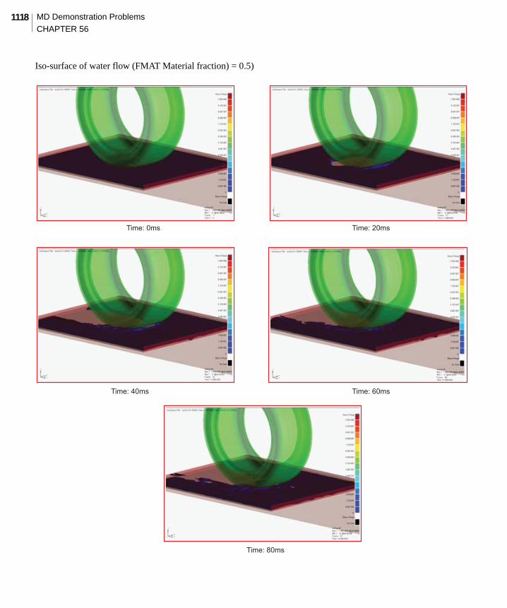
Iso-surface of water flow (FMAT Material fraction) = 0.5)

Time: 0ms Time: 20ms

Time: 60msTime: 40ms

Time: 80ms

1119CHAPTER 56

Hydroplaning Simulation

Postprocessing with SimXpertAfter the job is finished, there are two types of results: ARC and d3plot files. Both files are attached to SimXpert and are shown on the following pages.

a. For Default Workspace select MD Explicit

a

MD Demonstration Problems

CHAPTER 561120

Attach the Analysis Results File

a. File: Attach Results

b. For File Path, select the results file (attaching the d3plot file first)

c. Select the d3plot file.

d. Attach Options: click Both

e. Click Apply

f. Observe that the Lagrangian results are attached

a

cb

d

f

e

1121CHAPTER 56

Hydroplaning Simulation

Attach the Analysis Results File (continued)

a. For File Path, select the results file (to attach the ARC file)

b. Select the DYTR_EULER_0.ARC file

c.Attach Options: click Both

d. Click OK

e. Observe that the Outer Euler results are attached

a

e

d

bc

MD Demonstration Problems

CHAPTER 561122

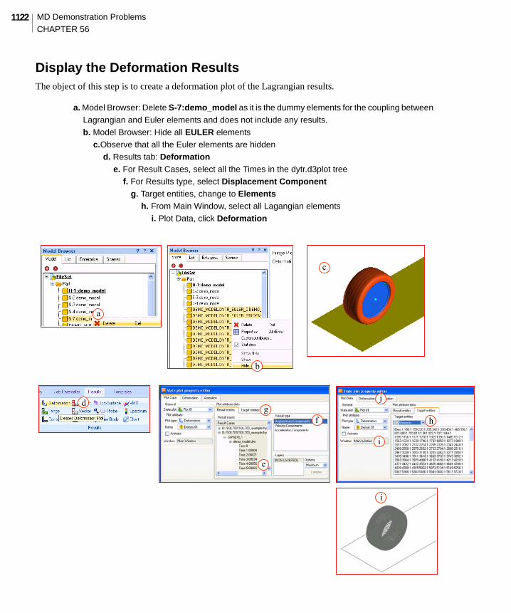
Display the Deformation ResultsThe object of this step is to create a deformation plot of the Lagrangian results.

a. Model Browser: Delete S-7:demo_model as it is the dummy elements for the coupling between

Lagrangian and Euler elements and does not include any results.

b. Model Browser: Hide all EULER elements

c.Observe that all the Euler elements are hidden

d. Results tab: Deformation

e. For Result Cases, select all the Times in the dytr.d3plot tree

f. For Results type, select Displacement Component

g. Target entities, change to Elements

h. From Main Window, select all Lagangian elements

i. Plot Data, click Deformation

c

d

e

fg

b

h

i

j

a

i

1123CHAPTER 56

Hydroplaning Simulation

Display the Deformation Results (continued)

a. Deformed display scaling, click True

b. Click Update

c.Check the deformation plot

b

c

a

MD Demonstration Problems

CHAPTER 561124

Display the Stress ResultsThe object of this step is to create a stress fringe plot of the Lagrangian results.

a. Model Browser: Show only Part H-1 and S-2 as Part3 and 4 are rigid and have not stress results.

b. Change Plot type to Fringe

c.Check the Result Cases to see that all the Times in the dytr.d3plot tree are selected

d. For Result type, select Stress Components

e. For Derivation, select von Mises

f. For Results entities, select Target entities

c

fe

d

b

a

1125CHAPTER 56

Hydroplaning Simulation

Display the Stress Results (continued)

a. Target entities, change to Elements

b. Select all the Lagangian Elements in the Main Window

c. Plot Data: Select Fringe

d. Element edge display: Display, select Element edges

e. Click Update

f. Check the stress fringe plot in the Main Window

c

edf

b

a

MD Demonstration Problems

CHAPTER 561126

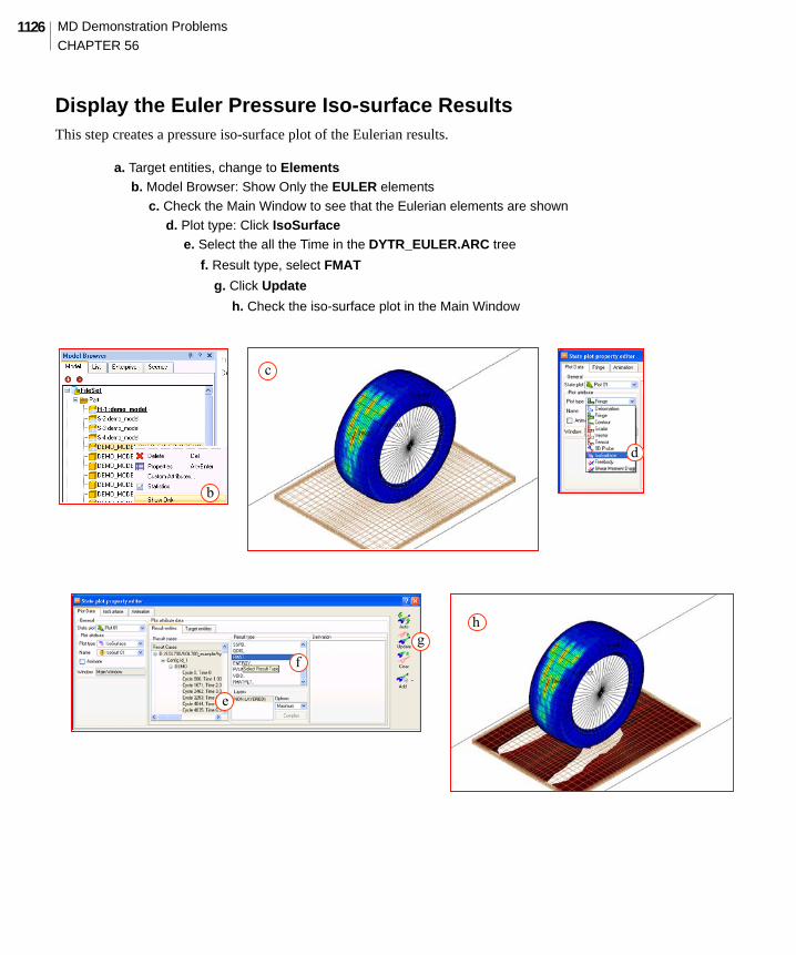
Display the Euler Pressure Iso-surface ResultsThis step creates a pressure iso-surface plot of the Eulerian results.

a. Target entities, change to Elements

b. Model Browser: Show Only the EULER elements

c. Check the Main Window to see that the Eulerian elements are shown

d. Plot type: Click IsoSurface

e. Select the all the Time in the DYTR_EULER.ARC tree

f. Result type, select FMAT

g. Click Update

h. Check the iso-surface plot in the Main Window

b

c

d

e

fg

h

1127CHAPTER 56

Hydroplaning Simulation

Display the Euler Pressure Iso-surface Results (continued)

a. FE Display: FE Shaded

b. Change the Transparency

a

b

MD Demonstration Problems

CHAPTER 561128

Make Animation

a. Click: Animation

b. Click Forward

ab

T= 0 ms T= 20 ms

1129CHAPTER 56

Hydroplaning Simulation

Animation (continued)

Input File(s)File Description

Hydro_planning_explicit.dat MD Nastran explicit input

Hydro_planning_explicit.pre_dytr.nastin MD Nastran initial stress and configuration information of explicit analysis for input to implicit analysis which is included in Hydro_planning_explicit.dat

Hydro_planning_implicit.bdf MD Nastran implicit model input which is included in Hydro_planning_explicit.dat

Hydro_planning_implicit.dat MD Nastran implicit input

T= 40 ms T= 60 ms

T= 80 ms

MD Demonstration Problems

CHAPTER 561130

VideoClick on the image or caption below to view a streaming video of this problem; it lasts approximately five minutes and explains how the post processing steps are performed.

Figure 56-3 Video of the Above Steps

Road

Tire and Wheel

Water