Image Compression Using Fractals and Wavelets · Image Compression Using Fractals and Wavelets ... A002 Final Report titled "Image Compression Using Fractals and Wavelets" ... 5.0

Image CompressionUsing Fractals and Wavelets

AD-A266 074

Final Report for the Phase II Contract

Sponsored by the Office of Naval Research

Contract No. N00014-91-C-0117

June 2, 1993

DTICAria E LECTE

Submitted To JUN 2 2 1993

Scientific Officer AnDr. Michael F. Shlesinger .

Attn: MFS, Code: 1112Office of Naval Research800 North Quincy StreetArlington, VA 22217-5000

NETROLOGIC Inc. • 5080 Shoreham Place, Suite 201 • San Diego, CA 92122Phone: (619) 625-6255 • Fax: (619) 625-6258

93 - DistribR 193-12957

* i&lIYr[ i H

Image CompressionUsing Fractals and Wavelets

Final Report for the Phase II Contract

Sponsored by the Office of Naval Research

Contract No. N00014-91-C-0117

Accesion For

NTIS CRA&I

June 2, 1993 DTIC -TABb;;3nhio-;ced l

Statement A per teleconMichael Shlesinger ONR/Code 1112 By. ............Arlington, VA 22217-5000 DitAibutioni

NWW 6/17/93 Availability CodesAvail and Ior

Dist SpecialSubmitted To

Scientific Officer d.l1Dr. Michael F. ShlesingerAttn: MFS, Code: 1112Office of Naval Research800 North Quincy StreetArlington, VA 22217-5000

NETROLOGIC Inc. • 5080 Shoreham Place, Suite 201 • San Diego, CA 92122Phone: (619) 625-6255 • Fax: (619) 625-6258

Acknowledgement

Mr. Dan Greenwood served as the project Principal Investigator. Dr. Albert Lawrence guided the

theoretical development of the Wavelet Compression study and Dr. Yuval Fisher guided the Fractal

Compression study. Mr. Fareed Stevenson, Mr. Richard Rea and Mr. Yaokun Zhong provided

software support. The encouragement and supervision of ONR's Dr. Shlesinger is greatly

appreciated by all the participants of this study.

Abstract

There are several approaches to image compression. The current most popular methods relies on

eliminating high frequency components of the signal by storing only the low frequency Fourier

coefficients. Other methods use a "building block" approach, breaking up images into a small

number of canonical pieces and storing only a reference to which piece goes where. Our research

has focused on a new scheme based on fractals. Our approach to image compression is to

tessellate the image with a tiling which varies with the local image complexity, and to check for self

similarity amongst the tiles. Self similarities are coded as systems of affine transformations which

can be stored far more compactly than the original images on small platforms.

An original objective of our Phal:, Ji research project was to develop a hardware implementation of

our Fractal based algorithm and to investigate various techniques for encoding. During the course

of initial investigations it became apparent that the bulk of our efforts should be directed toward

speeding up the software algorithms, especially in the decoding and adapting our fractal encoding

methods to color images. This is because the most significant commercial applications of image

compression require fast decoding.

Because the fractal compression method has not been entirely satisfactory for some types of images

such as maps, fingerprints and satellite images we have implemented a version of the wavelet

compression method reported by Antonini.

This encoding method has three main steps: a wavelet transform followed by a lattice vector

quantization followed by a Huffman encoding of the output vectors. The Huffman code step is not

reported in the report by Antonini. A standard codebook may be used for transmission, with a

provision for sending codebook entries for rarely-encountered vectors.

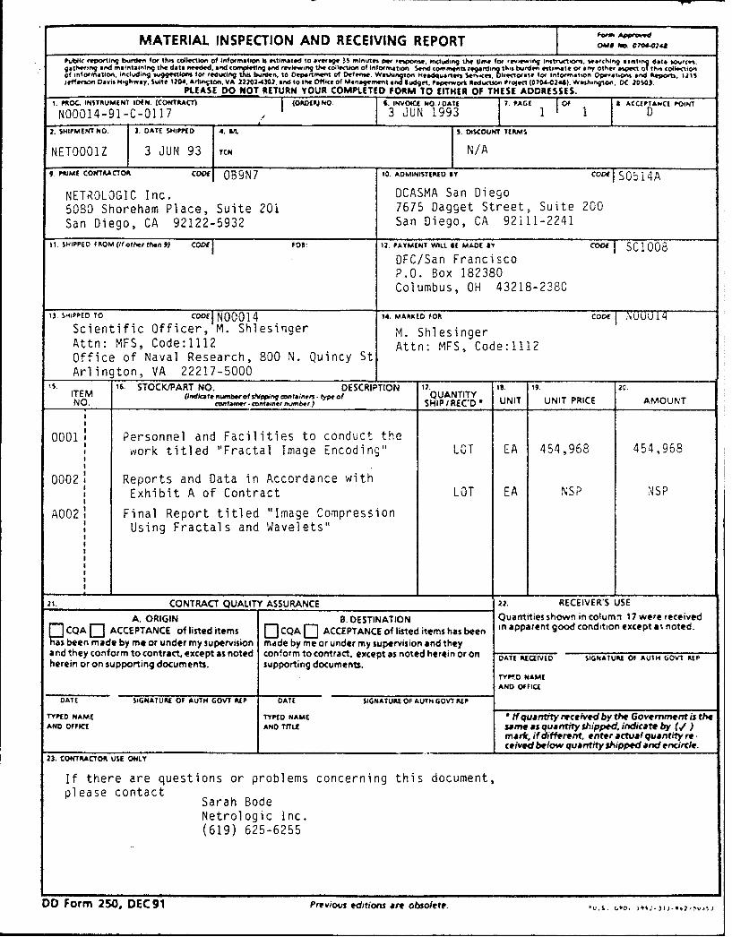
MATERIAL INSPECTION AND RECEIVING REPORTPubMik r rino l bj e bor ttiil Co0lletkon Of Information is itimated to aiveage 35 minrt- Per firooni Including the time for r•aiewinlg ins irutl•om. Wearching taftlin •.t. to ,"ga"'erIng an matalning the dat o need, ard completing and rtevewing the collection of Information Send commcenn regirdin this bwrden •tlmate o' any other .,oect o tt colwlvet•nof InfOrmation. ,n•ndihng vuggettont fof reducl 0 Department of Defene. Wat•hunton Heti•.tqer Serv•ces. Dirietorae for Information Opeut•o and Repom, 1t15Jeffeortni Davis Highway, Suite ?)A4, Arln;ltOn. VA 12202-4302. and to the Office of Managemenjt and Inudgit, Poperwort Reduciion Project (0704-024). Wavihnlon, DC 2OW03

PLEASE DO NOT RETURN YOUR COMPLETED FORM TO EITHER OF THESE ADDRESSES.

i. PROC. INSTRUMENT ID(N. (CONTRACT) I OPDIPJ No 1. INVOICE NO IOAU 7. PAGE 1Of 4 A(CCPTANCI 0-OINT

NOO014-91-C-0117 / 3 JUN 1993 1 1 Dz. SHIPMENT NO. 3. DATE SHIPPED 4. 54 5 DISCOUNT TERMS

NETOOO1Z 3 JUN 93 1ch N/A

. PRIME CONTRACTOR C OB9N7 t0. ADMINISTERED Y CoI S05 14A

NETROLOGIC Inc. DCASMA San Diego5080 Shoreham Place, Suite 201 7675 Dagget Street, Suite 200San Diego, CA 92122-5932 San Diego, CA 92111-2241

11. SHIPPED FROM (If other than 9) CODE FOS: 12. PAYMENT W"LL. Of MADE by co"E SCI1005

DFC/San FranciscoP.O. Box 182380Columbus, OH 43218-2380

13. SHIPPED TO CODE NO0014 14. MARKED FOR coDE NJUUU14

Scientific Officer, M. Shlesinger M. ShlesingerAttn: MFS, Code:1112 Attn: MFS, Code:1112Office of Naval Research, 800 N. Quincy StArlington, VA 22217-5000

5. 16. STOCK/PART NO. DESCRIPTION 17. Is. 19.ITEM (indkate n w eofsPpping wntainer¶. ypeof QUANTITYNO. container .containernumber) SHIP/REC*D * UNIT UNIT PRICE AMOUNT

0001 Personnel and Facilities to conduct thework titled "Fractal Image Encoding" LOT LA 454,968 454,968

0002: Reports and Data in Accordance withExhibit A of Contract LOT EA NSP NSP

A002 Final Report titled "Image CompressionUsing Fractals and Wavelets"

21. CONTRACT QUALITY ASSURANCE 32. RECEIVER'S USE

A. ORIGIN 8. DESTINATION Quantities shown in cotumn 17 were received

Fl CQA 0- ACCEPTANCE of listed items jCQA [] ACCEPTANCE of listed items has been in apparent good condition except a% noted.P been made by me or under my supervision made by me or under my supervision and theyand they conform to contract, except as noted conform to contract, except as noted herein or on DATE RECEiVED SIGNATURE Of AUIH GOVt REP

herein or on supporting documents. supporting documents.TYt.D NAME

AND OFFICE

DATE SIGNATURE OF AUTH GOVT OUP DATE SIGNATURE Of AUTH GOVT REP

rYPfD NAME TYPED NAME f quantfty received by the Govemrnment Is theAND OFFIleE AND TITLE same as quantity shipped indicate by (,/)

mat*, if different, enter actual quantity re.ceived below quantity shipped and encircde.

23. CONTRACTOR USE ONLY

If there are questions or problems concerning this document,please contact Sarah Bode

Netrologic Inc.(619) 625-6255

DO Form 250, DEC 91 Previous editions are obsolete. u.s. c,,. I4,-,2.v.,

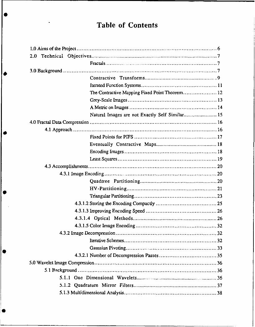
Table of Contents

1.0 Aims of the Project .................................................................................. 6

2.0 Technical Objectives ............................................................................... 7

Fractals ................................................................. 7

3.0 Background .......................................................................................... 7

Contractive Transforms ........................................... . 9Iterated Function Systems ............................................. I 1

The Contractive Mapping Fixed Point Theorem ................. 12

Grey-Scale Images ................................................... 13

A Metric on Images ................................................. 14

Natural Images are not Exactly Self Similar ..................... 15

4.0 Fractal Data Compression ......................................................................... 16

4.1 Approach ................................................................................... 16

Fixed Points for PIFS ............................................... 17

Eventually Contractive Maps ....................................... 18

Encoding Images ....................................................... 18

Least Squares ........................................................ 19

4.3 Accomplishments ............................................................................. 20

4.3.1 Image Encoding ................................................................... 20Quadtree Partitioning ............................................... 20

HV-Partitioning ...................................................... 21

Triangular Partitioning .............................................. 23

4.3.1.2 Storing the Encoding Compactly .................................... 25

4.3.1.3 Improving Encoding Speed .......................................... 26

4.3.1.4 Optical Methods ................................................... 26

4.3.1.5 Color Image Encoding ................................................ 32

4.3.2 Image Decompression ............................................................ 32

Iterative Schemes ..................................................... 32

Gaussian Pivoting ................................................... 334.3.2.1 Number of Decompression Passes .................................. 35

5.0 Wavelet Image Compression ...................................................................... 36

5.1 Background ................................................................................ 36

5.1.1 One Dimensional Wavelets ................................................... 36

5.1.2 Quadrature Mirror Filters .................................................... 37

5.1.3 Multidimensional Analysis ..................................................... 38

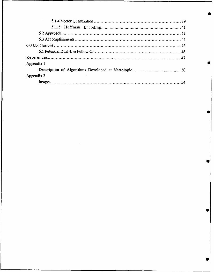
5.1.4 Vector Quantization ............................................................... 39

5.1.5 Huffman Encoding ............................................................ 41

5.2 A pproach ...................................................................................... 42

5.3 Accomplishments .......................................................................... 45

6.0 C onclusions ............................................................................................ 46

6.1 Potential Dual-Use Follow On .............................................................. 46

References ................................................................................................. 47

Appendix 1

Description of Algorithms Developed at Netrologic ....................................... 50

Appendix 2

Im ages ............................................................................................ 54

0

Figures and Tables

Figure 3-1 A copy machine that makes three reduced copies of the input image .......... 8

Figure 3-2 The first three copies generated on the copying machine of Figure 3-1 ....... 8

Figure 3-3 Transformations, their attractor, and a zoom on the attractor ............... 10

Figure 3-4 A graph generated from the Lena image ........................................... 13

Figure 3-5 The original 256 x 256 pixel Lena image ...................................... 14

Figure 3-6 Self similar portions of the Lena image ........................................ 15

Figure 4-1 A collie (256 x 256) compressed with the quadtree schente at 28.95 .......... 21

Figure 4-2 San Francisco (256 x 256)compressed with the HV scheme at 7.6 ..... 22

Figure 4-3 The HV scheme attempts to create self similar rectangles at different

scales .................................................................................... 22

Figure 4-4 A quadtree partition (5008 squares), and HV partition (2910 rectangles),

and a triangular partition (2954 triangles) ............................................. 23

Table 4-1 Two pseudo-codes for an adaptive encoding algorithm .......................... 24

Figure 4-5 256 x 256 Spierpinski triangle ................................................. 28

Figure 4-6 Grayscale optical result produced by convolution with a 4 x 4 square.

(Supplied by Foster-Miller) .......................................................... 29Figure 4-7 Grayscale optical result produced by convolution with a 8 x 8 square.

(Supplied by Foster-Miller) .......................................................... 30

Figure 4-8 Computer simulation of convolution - correlation of the Spierpinskitriangit. with the 4 x 4 square. (Supplied by Foster-Miller) ...................... 31

Figure 4-9 Computer simulation-correlation with 8 x 8 square .............................. 31

Table 4-2 Comparison of Phase I and Phase II Results ................................... 34

Table 4-3 Ratios vs. Passes ................................................................... 35

Table 5-1 Wavelet Filter Pairs ................................................................... 39

Table 5-2 Statistical Analysis of Wavelet Coefficients ........................................ 43

Figure 5-1 Adaptive Process for Scaling Wavelet Coefficients .............................. 44

Figure 5-2 Wavelet Compression Code ........................................................ 45

S

1.0 Aims of the Project

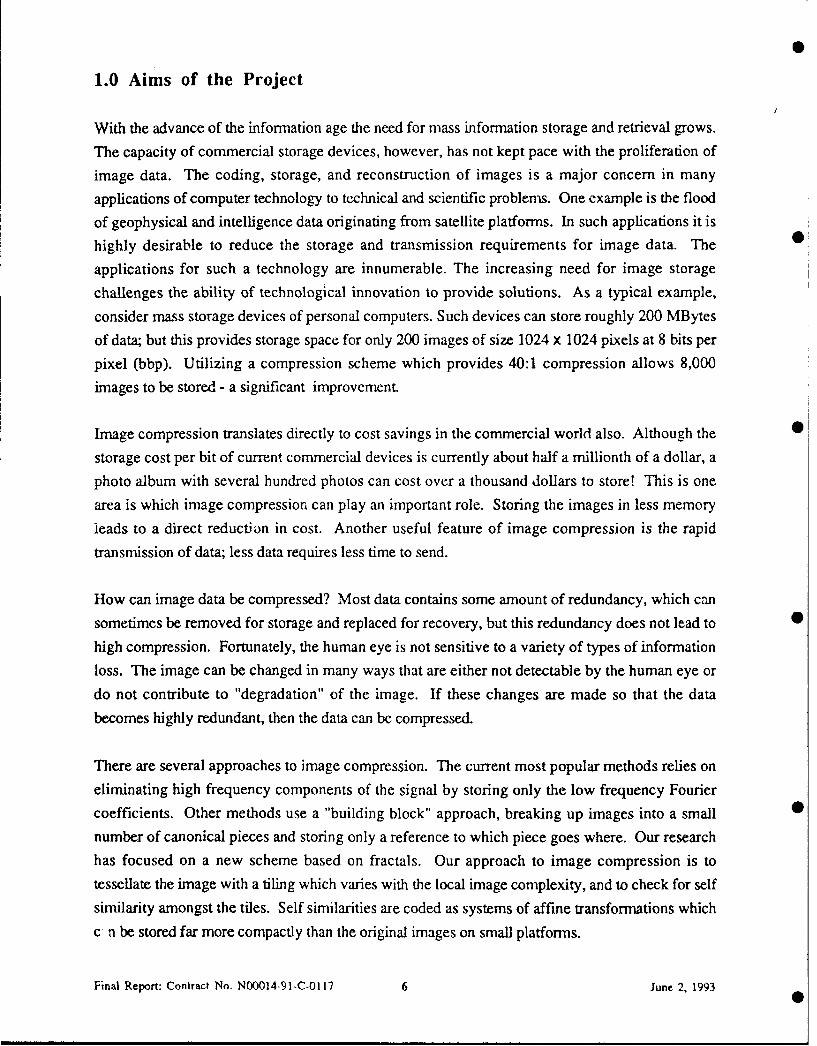
With the advance of the information age the need for mass information storage and retrieval grows.

The capacity of commercial storage devices, however, has not kept pace with the proliferation of

image data. The coding, storage, and reconstruction of images is a major concern in many

applications of computer technology to technical and scientific problems. One example is the flood

of geophysical and intelligence data originating from satellite platforms. In such applications it is

highly desirable to reduce the storage and transmission requirements for image data. The

applications for such a technology are innumerable. The increasing need for image storage

challenges the ability of technological innovation to provide solutions. As a typical example,

consider mass storage devices of personal computers. Such devices can store roughly 200 MBytes

of data; but this provides storage space for only 200 images of size 1024 x 1024 pixels at 8 bits per

pixel (bbp). Utilizing a compression scheme which provides 40:1 compression allows 8,000

images to be stored - a significant improvement.

Image compression translates directly to cost savings in the commercial world also. Although the

storage cost per bit of current commercial devices is currently about half a millionth of a dollar, a

photo album with several hundred photos can cost over a thousand dollars to store! This is one

area is which image compression can play an important role. Storing the images in less memory

leads to a direct reduction in cost. Another useful feature of image compression is the rapid

transmission of data; less data requires less time to send.

How can image data be compressed? Most data contains some amount of redundancy, which can

sometimes be removed for storage and replaced for recovery, but this redundancy does not lead to

high compression. Fortunately, the human eye is not sensitive to a variety of types of information

loss. The image can be changed in many ways that are either not detectable by the human eye or

do not contribute to "degradation" of the image. If these changes are made so that the data

becomes highly redundant, then the data can be compressed.

There are several approaches to image compression. The current most popular methods relies on

eliminating high frequency components of the signal by storing only the low frequency Fourier

coefficients. Other methods use a "building block" approach, breaking up images into a small

number of canonical pieces and storing only a reference to which piece goes where. Our research

has focused on a new scheme based on fractals. Our approach to image compression is to

tessellate the image with a tiling which varies with the local image complexity, and to check for self

similarity amongst the tiles. Self similarities are coded as systems of affine transformations which

c n be stored far more compactly than the original images on small platforms.

Final Report: Contract No. N00014-91-C-0117 6 June 2. 1993

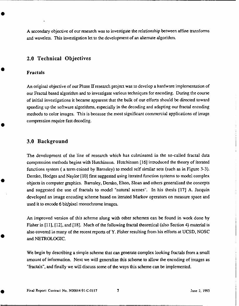
A secondary objective of our research was to investigate the relationship between affine transforms

and wavelets. This investigation let to the development of an alternate algorithm.

2.0 Technical Objectives

Fractals

An original objective of our Phase Ir research project was to develop a hardware implementation of

our Fractal based algorithm and to investigate various techniques for encoding. During the course

of initial investigations it became apparent that the bulk of our efforts should be directed toward

speeding up the software algorithms, especially in the decoding and adapting our fractal encoding

methods to color images. This is because the most significant commercial applications of image

compression require fast decoding.

3.0 Background

The development of the line of research which has culminated in the so-called fractal data

compression methods begins with Hutchinson. Hutchinson [16] introduced the theory of iterated

functions system ( a term coined by Barnsley) to model self similar sets (such as in Figure 3-3).

Demko, Hodges and Naylor [10] first suggested using iterated function systems to model complex

objects in computer graphics. Barnsley, Demko, Elton, Sloan and others generalized the concepts

and suggested the use of fractals to model "natural scenes". In his thesis [17] A. Jacquin

developed an image encoding scheme based on iterated Markov operators on measure space and

used it to encode 6 bit/pixel monochrome images.

An improved version of this scheme along with other schemes can be found in work done by

Fisher in [11], [12], and [181. Much of the following fractal theoretical (also Section 4) material is

also covered in many of the recent reports of Y. Fisher resulting from his efforts at UCSD, NOSC

and NETROLOGIC.

We begin by describing a simple scheme that can generate complex looking fractals from a small

amount of information. Next we will generalize this scheme to allow the encoding of images as

"fractals", and finally we will discuss some of the ways this scheme can be implemented.

Final Report: Contract No. N00014-91-C-0117 7 June 2, 1993

O

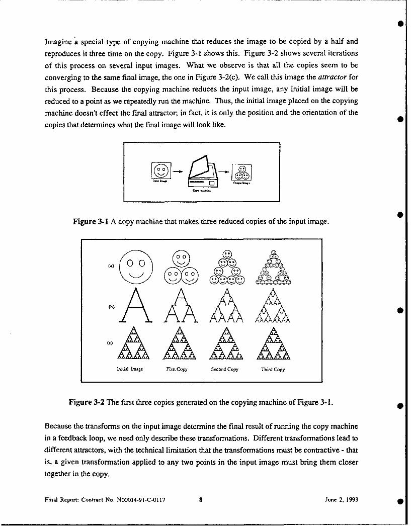
Imagine a special type of copying machine that reduces the image to be copied by a half and

reproduces it three time on the copy. Figure 3-1 shows this. Figure 3-2 shows several iterations

of this process on several input images. What we observe is that all the copies seem to be

converging to the same final image, the one in Figure 3-2(c). We call this image the attractor for

this process. Because the copying machine reduces the input image, any initial image will be

reduced to a point as we repeatedly run the machine. Thus, the initial image placed on the copying

machine doesn't effect the final attractor; in fact, it is only the position and the orientation of the

copies that determines what the final image will look like. •

000

Figure 3-1 A copy machine that makes three reduced copies of the input image.

(a)(5000

(c)

---

Initial Image First Copy Second Copy Thid Copy

Figure 3-2 The first three copies generated on the copying machine of Figure 3-1.

Because the transforms on the input image determine the final result of running the copy machinein a feedback loop, we need only describe these transformations. Different transformations lead to

different attractors, with the technical limitation that the transformations must be contractive - thatis, a given transformation applied to any two points in the input image must bring them closer

together in the copy.


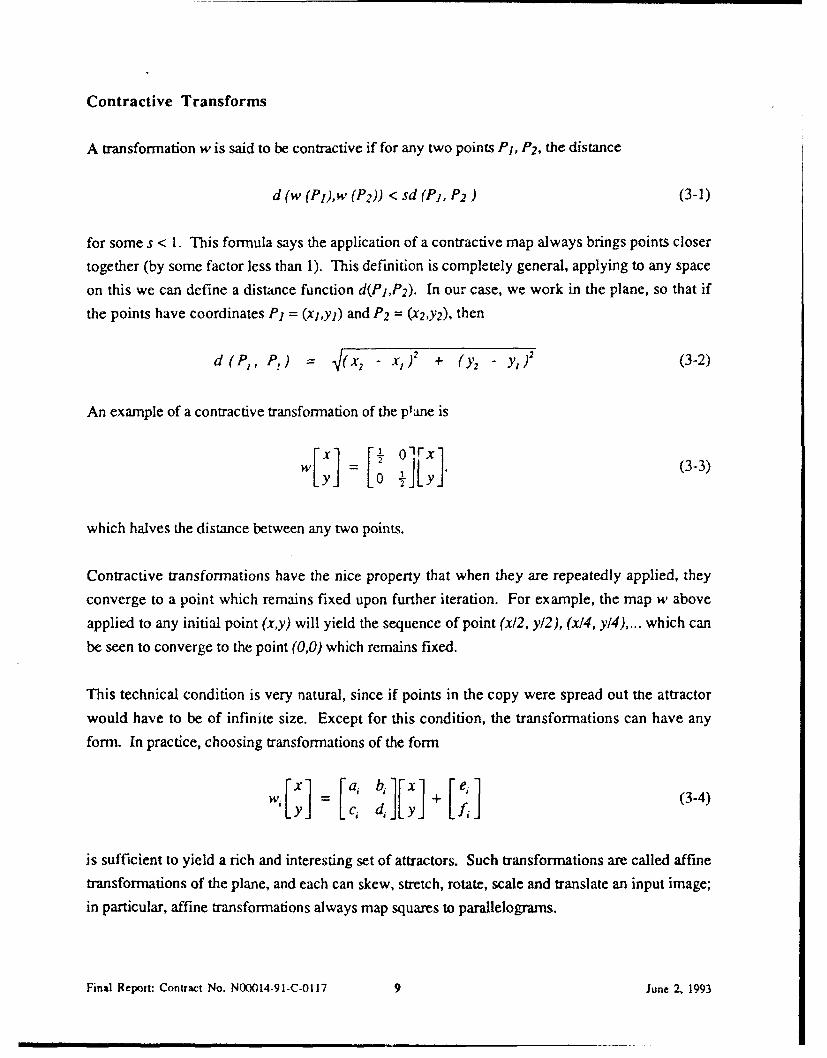
Contractive Transforms

A transformation w is said to be contractive if for any two points P1 , P2, the distance

d (w (P1),w (P2)) < sd (P1, P2) (3-1)

for some s < 1. This formula says the application of a contractive map always brings points closer

together (by some factor less than 1). This definition is completely general, applying to any space

on this we can define a distance function d(PIP 2). In our case, we work in the plane, so that if

the points have coordinates P1 = (xl,yl) and P2 = (x2,Y2), then

d(P, PF,) = (x _ x) 2 + (Y2 _ Yj (3-2)

An example of a contractive transformation of the plane is

w[x] = [2, Ojrx (3-3)

which halves the distance between any two points.

Contractive transformations have the nice property that when they are repeatedly applied, they

converge to a point which remains fixed upon further iteration. For example, the map w above

applied to any initial point (x,y) will yield the sequence of point (x/2, y/2), (x14, y/4 ).... which can

be seen to converge to the point (0,0) which remains fixed.

This technical condition is very natural, since if points in the copy were spread out the attractor

would have to be of infinite size. Except for this condition, the transformations can have any

form. In practice, choosing transformations of the form

LY cý. d, JyJ f(-4

is sufficient to yield a rich and interesting set of attractors. Such transformations are called affine

transformations of the plane, and each can skew, stretch, rotate, scale and translate an input image;

in particular, affine transformations always map squares to parallelograms.


30

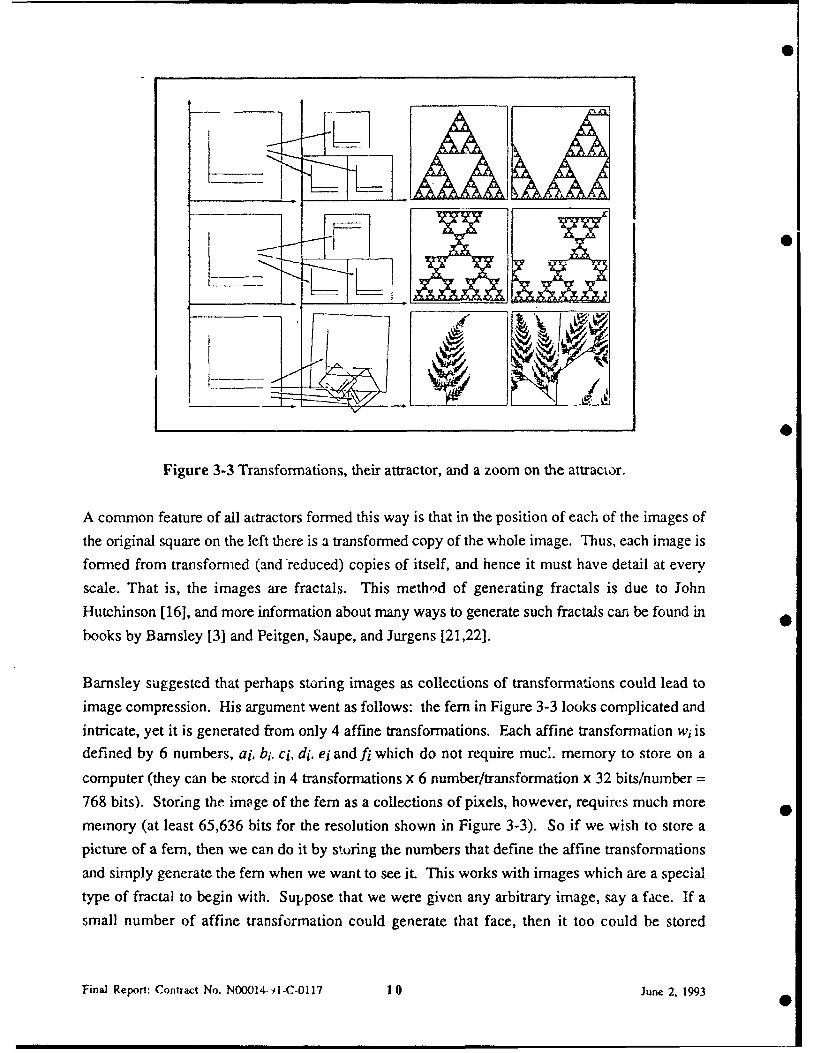
Figure 3-3 Transformations, their attractor, and a zoom on the attractor.

A common feature of all attractors formed this way is that in the position of each of the images of

the original square on the left there is a transformed copy of the whole image. Thus, each image is

formed from transformed (and *reduced) copies of itself, and hence it must have detail at every

scale. That is, the images are fractals. This method of generating fractals is due to JohnHutchinson [161, and more information about many ways to generate such fractals can be found in

books by Barnsley [3] and Peitgen, Saupe, and Jurgens [21,22].

Barnsley suggested that perhaps storing images as collections of transformations could lead to

image compression. His argument went as follows: the fern in Figure 3-3 looks complicated and

intricate, yet it is generated from only 4 affine transformations. Each affine transformation wi isdefined by 6 numbers, ai, bi. ci, di, ei and fi which do not require mucX. memory to store on a

computer (they can be storcd in 4 transformations x 6 number/transformation x 32 bits/number =

768 bits). Storing the image of the fern as a collections of pixels, however, requires much more

memory (at least 65,636 bits for the resolution shown in Figure 3-3). So if we wish to store apicture of a fern, then we can do it by sturing the numbers that define the affine transformations

and simply generate the fern when we want to see it. This works with images which are a special

type of fractal to begin with. Suppose that we were given any arbitrary image, say a face. If a

small number of affine transformation could generate that face, then it too could be stored

Final Report: Contract No. NOOO]4.iI-C-0117 10 June 2, 1993

compactly. The trick is finding those numbers. Unfortunately we can only apprnximate an image

in this way.

Before we discuss the problem of approximating an image by a system of affine transforms we

will set up some machinery for describing these systems.

Iterated Function Systems

Running the special copy machine in a feedback loop is a metaphor for a mathematical model called

an iterated function system (IFS). An iterated function system consists of a collection of

contractive transformations {wi: -- R 2 1 i = 1,...n} which map the plane R2 to itself. This

collection of transformations defines a map

w(.)= U=I w(.)(3-5)

The map W is not applied to the plane, it is applied to sets - that is, collections of points in the

plane. Given an input set S, we can compute wi (S) for each i, take the union of these sets, and get

a new set W(S). So W is a map on the space of subsets of the plane. We will call a subset of the

plane an image, because the set defines an image when the points in the set are drawn in black, and

because later we will want to use the same notation on graphs of functions which will representactual images. An important fact proved by Hutchinson is that when the wi are contractive in the

plane, then W is contractive in a space of (closed and bounded) subsets of the plane. Hutchinson's

theorem allows us to use the contractive mapping fixed point theorem which tells us that the map

W will have a unique fixed point in the space of all images. That is, whatever image (or set) we

start with, we can repeatedly apply W to it and we will converge to a fixed image. Thus W (or the

wi) completely determine a unique image.

In other words, given an input image fo, we can run the copying machine once to get f] = W(fo),twice to get f2 = W(f 1 ) = W(W(fo)) -= W02(fo), and so on. The attractor, which is the result of

running the copying machine in a feedback loop, is the limit set

IWI=-f_ = lim W 0'(f 0 )IW f*n •* - (3-6)

which is not dependent on the choice of fo. Iterated function systems are interesting in their own

right, but we are not concerned with them specifically. We will generalize the idea of the copy

Final Report: Contract No. N00014-91-C-0117 1 1 June 2. 1993

machine and use it to encode grey-scale images; that is, images that are not just black and white but

which contain shades of grey as wvell.

The Contractive Mapping Fixed Point Theorem

The contractive mapping fixed point theorem says that something that is intuitively obvious: if a

map is contractive then when we apply it repeatedly starting with any initial point we converge to a

unique fixed point, for example, the map w(x) = x/2 on the real line is contractive for the normal

metric d(xy) =/x-y/, because the distance between w(x) and w(y) is half the distance between x

and y. Furthermore, if we iterate w from any initial point x, we get a sequence of points x12,

x/4,... that converges to the fixed point 0.

This theorem tells us when we can expect a collection of transformations to define images. Let's

write it precisely and examine it carefully.

THE CONTRACTIVE MAPPING FIXED POINT THEOREM. If X is a complete metric space

and W :X -X is contractive, then W has a unique fixed point /W/.

A complete metric space is a "gap-less" space on which we can measure the distance between any

two points. For example, the real line is a complete metric space with distance between any two

points x and y given by /x-y/. The set of all fractions of integers, however, is not complete. We

can measure the distance between two fractions in the same way, but between any two elements of

the space we find a real number (that is, a "gap") which is not a fraction and hence is not in the

space. Returning to our example, the map w can operate on the space of fractions, however the

map x ,-- x cannot. This map is contractive, but after one application of the map we are no

longer in the same space we began in. This is the reason for requiring that we work in a complete

metric space.

A fixed point 1W / e X of W is a point that satisfies W(/W/) = /WI. Our mapping w(x) = x/2 on

the real line has a unique fixed point: Start with an arbitrary point x e X. Now iterate W to get a

sequence of points x,W(x), W(W(x),... The distance between W(x) and W(W(x)) is less by some

factor s < 1 than the dista: ;e between x and W(x). At each step the distance to the next point is

less by some factor than the distance to the previous point. Because we are taking geometrically

smaller steps, and since our space has no gaps, we must eventually converge to a point in the space

which we denote 1W/ = limn .,,, W0" (x). This point is fixed, because applying W one more time

is the same as starting at W(x) instead of x, and either way we get to the same point.


The fixed-point is unique because if we assume that there are two, then we will get a contradiction:

Suppose there are two fixed points xj and x2; then the distance between W(xl) and W(x2), which

is the distance between xl and x2; this is a contradiction.

Thus, the main result we have demonstrated is that when W is contractive, we get a fixed point

IWI = lim W*n (x)n • ,(3-7)

for any initial x.

Grey-Scale Images

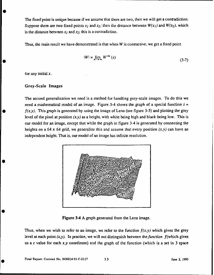
The second generalization we need is a method for handling grey-scale images. To do this we

need a mathematical model of an image. Figure 3-4 shows the graph of a special function z =

f(x,y). This graph is generated by using the image of Lena (see figure 3-5) and plotting the grey

level of the pixel at position (xy) as a height, with white being high and black being low. This is

our model for an image, except that while the graph in figure 3-4 is generated by connecting the

heights on a 64 x 64 grid, we generalize this and assume that every position (x,y) can have an

independent height. That is, our model of an image has infinite resolution.

SP

Figure 3-4 A graph generated from the Lena image.

Thus, when we wish to refer to an image, we refer to the function f(x,y) which gives the grey

level at each point (xy). In practice, we will not distinguish between the function f(which gives

us a z value for each x,y coordinate) and the graph of the function (which is a set in 3 space

Final Report: Contract No. N00014-91-C-0117 13 June 2 1993

consisting of the points in the surface defined by f) For simplicity, we assume we are dealing with

square images of size 1; that is, (x,y) e ((u,v) : 0 •5 u,v <_ 1 -=12 , and f (xy) e I = [0,11. We

have introduced some convenient notation here: I means the interval 10,11 and 2 is the unit square.

A Metric on Images

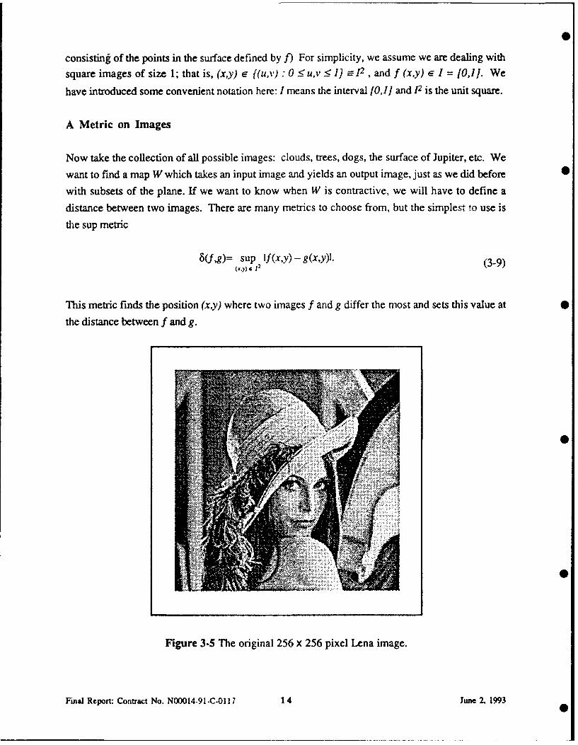
Now take the collection of all possible images: clouds, trees, dogs, the surface of Jupiter, etc. We

want to find a map W which takes an input image and yields an output image, just as we did before

with subsets of the plane. If we want to know when W is contractive, we will have to define a

distance between two images. There are many metrics to choose from, but the simplest to use is

the sup metric

W(,g)= sup If(x,y)-g(x,y).((-.y)E e 2 (3-9)

This metric finds the position (xy) where two images f and g differ the most and sets this value at •

the distance between f and g.

zS

0

Figure 3-5 The original 256 x 256 pixel Lena image.

Final Report: Contract No. N00014-91 -C-0117 14 June 2, 1993

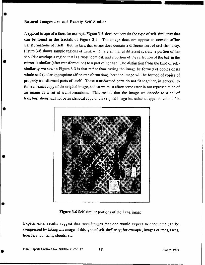
Natural Images are not Exactly Self Similar

A typical image of a face, for example Figure 3-5, does not contain the type of self-similarity thatcan be found in the fractals of Figure 3-3. The image does not appear to contain affinetransformations of itself. But, in fact, this image does contain a different sort of self-similarity.Figure 3-6 shows sample regions of Lena which are similar at different scales: a portion of hershoulder overlaps a region that is almost identical, and a portion of the reflection of the hat in themirror is similar (after transformation) to a part of her hat. The distinction from the kind of self-similarity we saw in Figure 3-3 is that rather than having the image be formed of copies of itswhole self (under appropriate affine transformation), here the image will be formed of copies ofproperly transformed parts of itself. These transformed parts do not fit together, in general, toform an exact copy of the original image, and so we must allow some error in our representation ofan image as a set of transformations. This means that the image we encode as a set oftransformations will not be an identical copy of the original image but rather an approximation of it.

0u

Figure 3-6 Self similar portions of the Lena image.

Experimental results suggest that most images that one would expect to encounter can becompressed by taking advantage of this type of self-similarity; for example, images of trees, faces,

houses, mountains, clouds, etc.


4.0 Fractal Data Compression

4.1 Approach

Our approach to fractal data compression is to partition the image. This may be described in termsof the copying machine metaphor introduced in the background section. The partitioned copymachine has four variable components:

0

"• the number of copies of the original pasted together to form the output,"* a setting of position and scaling, stretching, skewing and rotation factors for each copy.

These features are a part of the copying machine that can be used to generate the images in Figure3-3. We add to the following two capabilities:

"• a contrast and brightness adjustment for each copy,"• a mask which selects, for each copy, a part of the original to be copied. 0

These extra variables are sufficient to allow the encoding of grey-scale images. The last partitionsan image into pieces which are each transformed separately. By partitioning the image into pieces,

we allow the encoding of many shapes that are difficult to encode using an IFS.

Let us review what happens when we copy an original image using this machine. Each lens selectsa portion of the original, which we denote by Di and copies that part (with a brightness andcontrast transformation) to a part of the produced copy which is denoted Ri. We call Di domainsand the Ri ranges. We denote this transformation by wi. The partitioning is implicit in the

notation, so that we can use almost the same notation as with an IFS. Given an image f, onecopying step in a machine with N lenses can be written as W(f) = wl(f),'w2 (f)u....,WN (f).

As before the machine runs in a feedback loop; its own output is fed back as its new input again

and again.

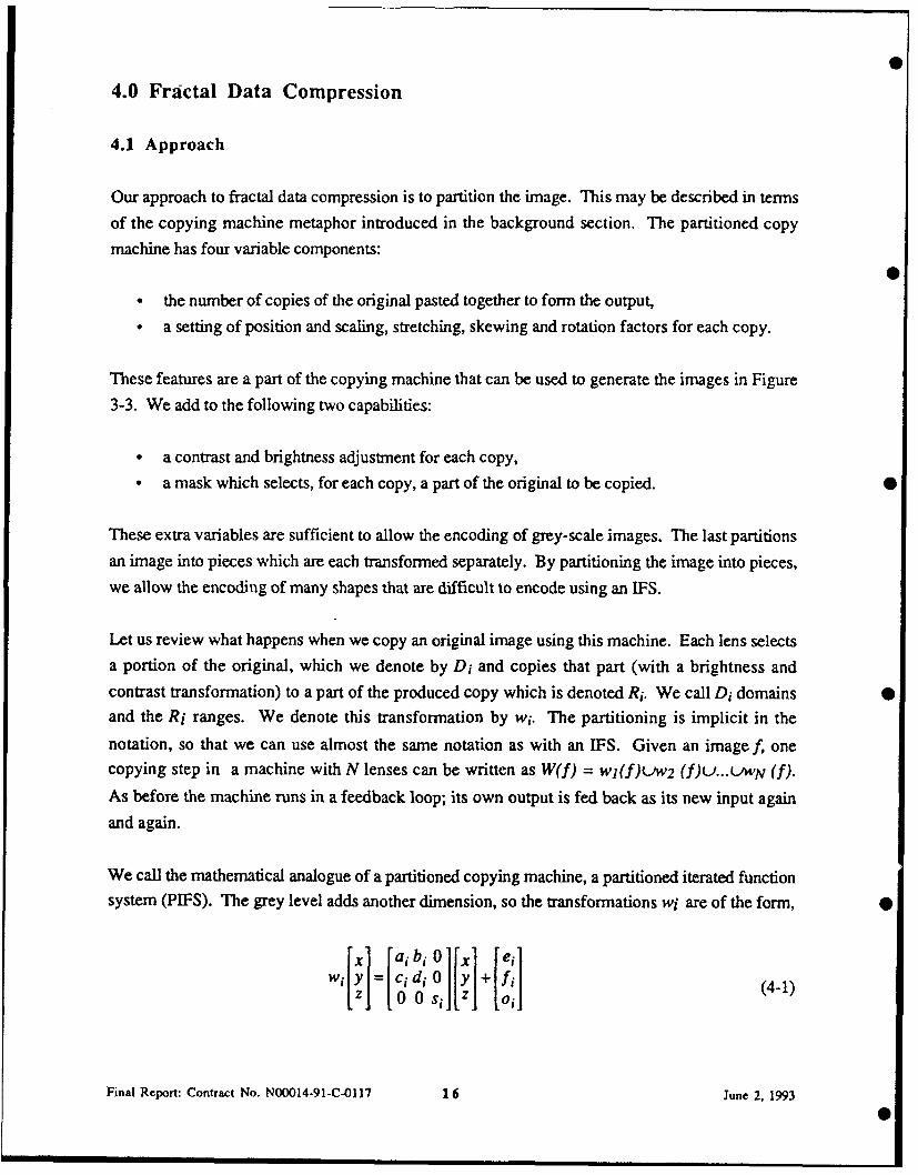
We call the mathematical analogue of a partitioned copying machine, a partitioned iterated functionsystem (PIFS). The grey level adds another dimension, so the transformations wi are of the form, •,xl= 0ai l x1+1il

wi y ccidiO y + i (4-1)

Final Report: Contract No. N00014-91-C-0117 1 6 June 2. 1993

0

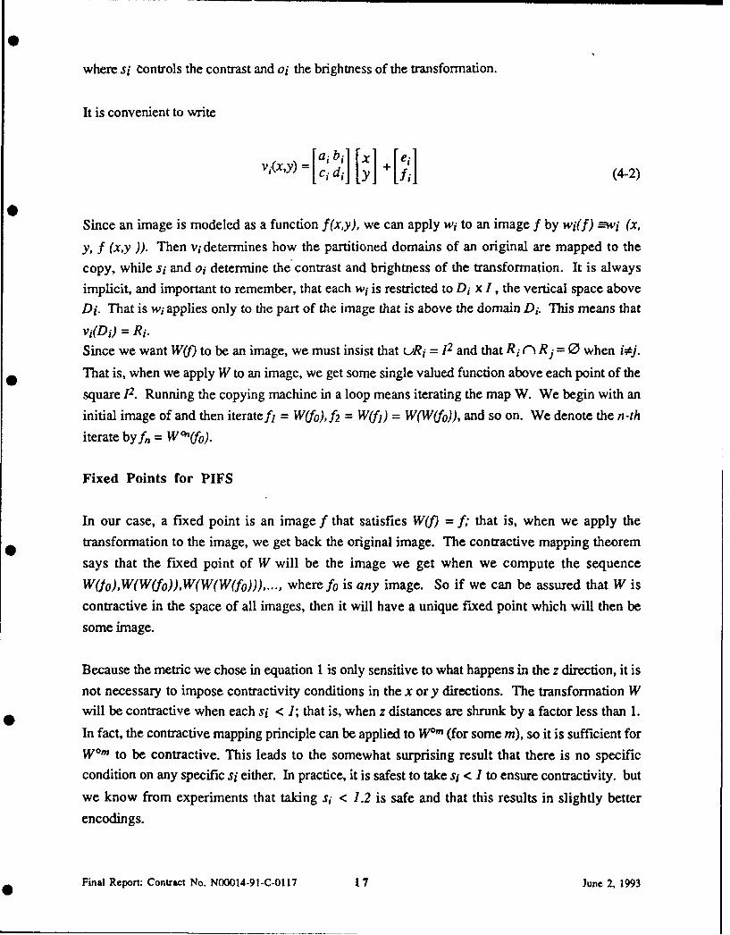
where si controls the contrast and oi the brightness of the transformation.

It is convenient to write

Since an image is modeled as a function f(x,y), we can apply wi to an image f by wi(f) =-wi (x,

y, f (x,y )). Then vi determines how the partitioned domains of an original are mapped to the

copy, while si and oi determine the contrast and brightness of the transformation. It is always

implicit, and important to remember, that each wi is restricted to Di X I, the vertical space above

Di. That is wi applies only to the part of the image that is above the domain Di. This means that

vi(Di) = Ri.

Since we want W(.) to be an image, we must insist that cRi = 12 and that Ri r) Rj = 0 when itj.

That is, when we apply W to an image, we get some single valued function above each point of the

square 12. Running the copying machine in a loop means iterating the map W. We begin with an

initial image of and then iteratefl = W(fo),f 2 = W(fl) = W(W(fo)), and so on. We denote the n-th

iterate byf, = Wn(fo).

Fixed Points for PIFS

In our case, a fixed point is an image f that satisfies W(f) = f; that is, when we apply the

transformation to the image, we get back the original image. The contractive mapping theorem

says that the fixed point of W will be the image we get when we compute the sequence

W(jo),W(W(fo)),W(W(W(fo))),..., where fo is any image. So if we can be assured that W is

contractive in the space of all images, then it will have a unique fixed point which will then be

some image.

Because the metric we chose in equation 1 is only sensitive to what happens in the z direction, it is

not necessary to impose contractivity conditions in the x or y directions. The transformation Wwill be contractive when each si < 1; that is, when z distances are shrunk by a factor less than 1.

In fact, the contractive mapping principle can be applied to W"'' (for some m), so it is sufficient for

Wom to be contractive. This leads to the somewhat surprising result that there is no specificcondition on any specific si either. In practice, it is safest to take sl < 1 to ensure contractivity. but

we know from experiments that taking si < 1.2 is safe and that this results in slightly better

encodings.


Eventually Contractive Maps

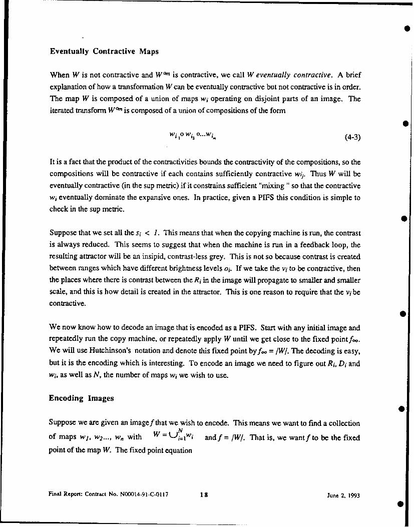
When W is not contractive and W1- is contractive, we call W eventually contractive. A brief

explanation of how a transformation W can be eventually contractive but not contractive is in order.The map W is composed of a union of maps wi operating on disjoint parts of an image. Theiterated transform Wn is composed of a union of compositions of the form

Wi 1° wi2 °."wi (4-3)

It is a fact that the product of the contractivities bounds the contractivity of the compositions, so the

compositions will be contractive if each contains sufficiently contractive wip. Thus W will beeventually contractive (in the sup metric) if it constrains sufficient "mixing" so that the contractivewi eventually dominate the expansive ones. In practice, given a PIFS this condition is simple to

check in the sup metric.

Suppose that we set all the si < 1. This means that when the copying machine is run, the contrastis always reduced. This seems to suggest that when the machine is run in a feedback loop, theresulting attractor will be an insipid, contrast-less grey. This is not so because contrast is created

between ranges which have different brightness levels oi. If we take the vi to be contractive, thenthe places where there is contrast between the Ri in the image will propagate to smaller and smallerscale, and this is how detail is created in the attractor. This is one reason to require that the vi be

contractive.0

We now know how to decode an image that is encoded as a PIFS. Start with any initial image andrepeatedly run the copy machine, or repeatedly apply W until we get close to the fixed point f*.

We will use Hutchinson's notation and denote this fixed point byf,,, = IWI. The decoding is easy,

but it is the encoding which is interesting. To encode an image we need to figure out Ri, Di and

wi, as well as N, the number of maps wi we wish to use.

Encoding Images0

Suppose we are given an imagef that we wish to encode. This means we want to find a collectionN

of maps wl, w2 ..., w,, with W = U1 i.lWi andf = /W!. That is, we wantf to be the fixed

point of the map W. The fixed point equation


0

f= w(f) = wl(f) u W2 (f) C-...wN(f) (4-4)

suggests how this may be achieved. We seek a partition of f into pieces to which we apply the

transforms wi and get back f. This is too much to hope for in general, since images are not

composed of pieces that can be transformed non-trivially to fit exactly somewhere else in the

image. What we can hope to find is another image f'= IWI with d(f'fj) small. That is we seek a

transformation W whose fixed point f' = /W is close to, or looks like, f. In that case,

f f' =W(f) = w(f) = wI(f) U w2(f) U...wN(f). (4-5)

Thus it is sufficient to approximate the parts of the image with transformed pieces. We do this by

minimizing the following quantities

d(fr(RI x I), wi(f)) i = 1,...,N (4-6)

That is, we find pieces Di and maps wi, so that when we apply a wi to the part of the image over

Di, we get something that is very close to the part of the image over Ri. Finding the pieces Ri (and

corresponding Di) is the heart of the problem.

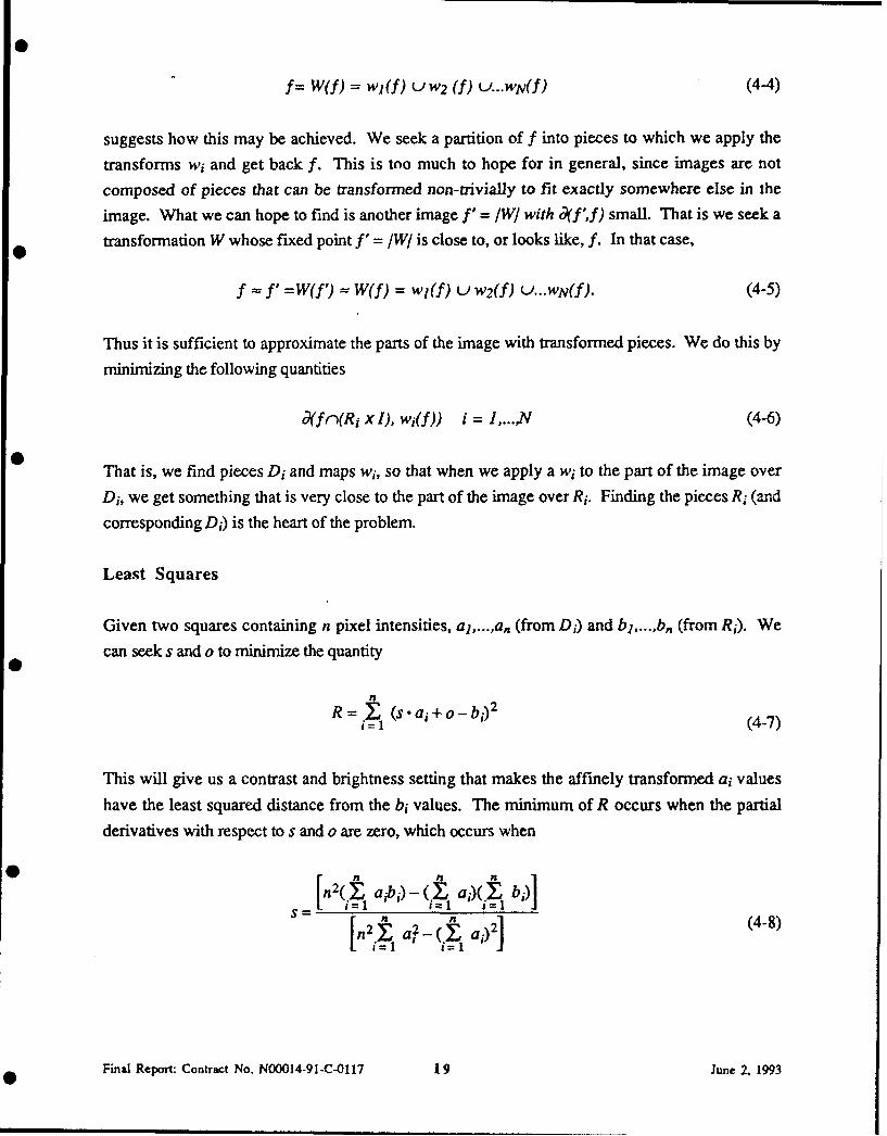
Least Squares

Given two squares containing n pixel intensities, aj,....an (from Di) and bl,...,bn (from R5). We

can seek s and o to minimize the quantity

0n

R= (s'ai+o-bi)2i = (4-7)

This will give us a contrast and brightness setting that makes the affinely transformed ai values

have the least squared distance from the bi values. The minimum of R occurs when the partial

derivatives with respect to s and o are zero, which occurs when

n[2( i aibi) - (Y, ai)(iZ bi)]


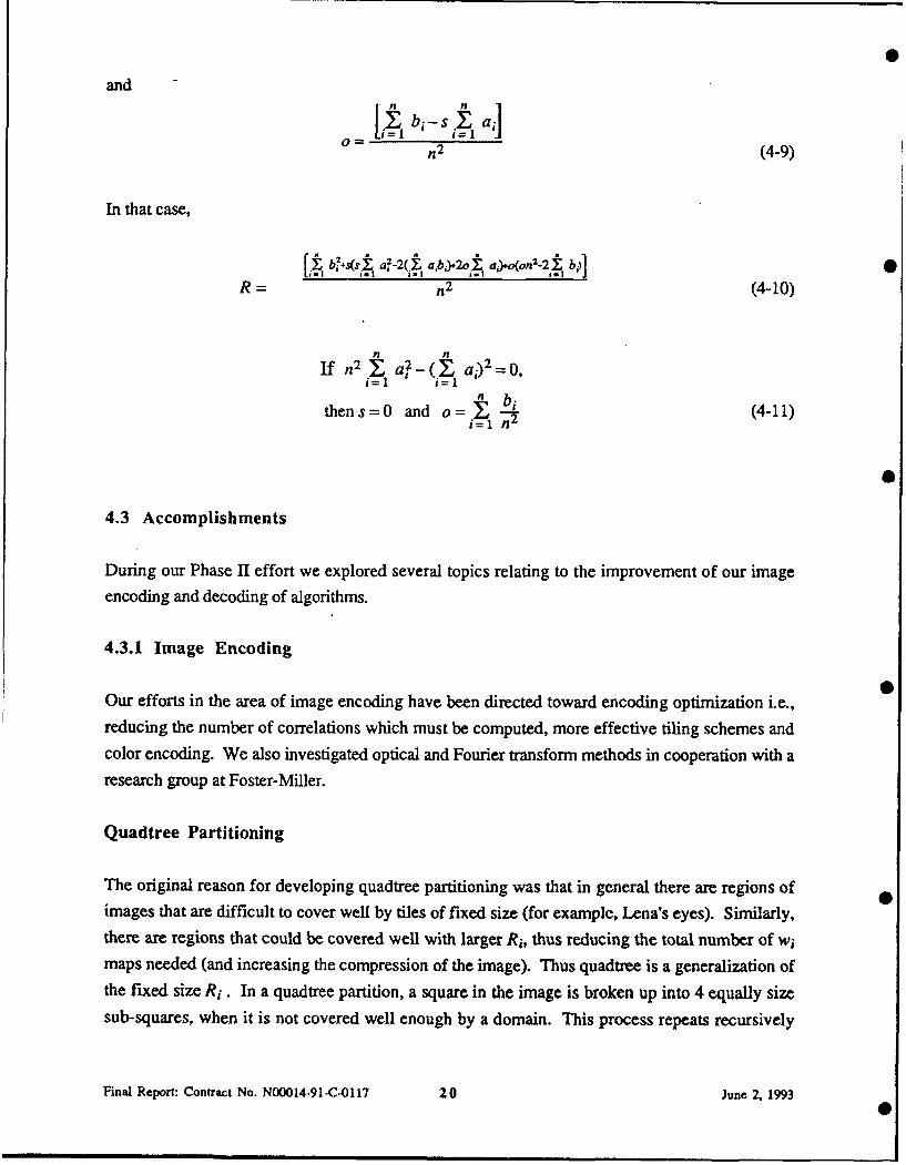
and

[i b-s~ a]n2 (4-9)

In that case,

[tbý.S(sy, aý-b ,h>.2.o ; a,).oon2-2j Zjf-, i- iz i,,R =n2 (4-10)

n n

If n2 l a2-(_ ai)2 =0,n x bi (- 1

thens=0 and o=X I (4-11)

4.3 Accomplishments

During our Phase II effort we explored several topics relating to the improvement of our imageencoding and decoding of algorithms.

4.3.1 Image Encoding

40Our efforts in the area of image encoding have been directed toward encoding optimization i.e.,reducing the number of correlations which must be computed, more effective tiling schemes andcolor encoding. We also investigated optical and Fourier transform methods in cooperation with a

research group at Foster-Miller.

Quadtree Partitioning

The original reason for developing quadtree partitioning was that in general there are regions ofimages that are difficult to cover well by tiles of fixed size (for example, Lena's eyes). Similarly,there are regions that could be covered well with larger Ri, thus reducing the total number of wimaps needed (and increasing the compression of the image). Thus quadtree is a generalization ofthe fixed size Ri. In a quadtree partition, a square in the image is broken up into 4 equally sizesub-squares, when it is not covered well enough by a domain. This process repeats recursively


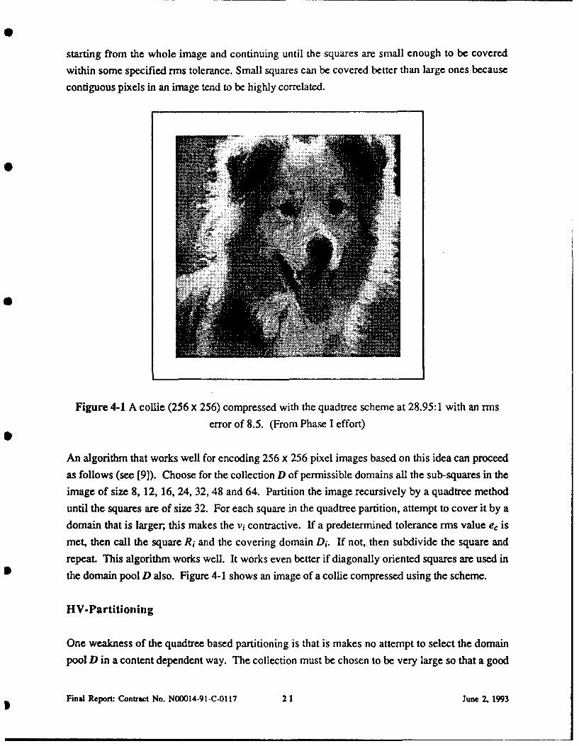
starting from the whole image and continuing until the squares are small enough to be covered

within some specified rms tolerance. Small squares can be covered better than large ones because

contiguous pixels in an image tend to be highly correlated.

Figure 4-1 A collie (256 x 256) compressed with the quadtree scheme at 28.95:1 with an rms

error of 8.5. (From Phase I effort)

An algorithm that works well for encoding 256 x 256 pixel images based on this idea can proceed

as follows (see [9]). Choose for the collection D of permissible domains all the sub-squares in the

image of size 8, 12, 16, 24, 32, 48 and 64. Partition the image recursively by a quadtree method

until the squares are of size 32. For each square in the quadtree partition, attempt to cover it by a

domain that is larger;, this makes the vi contractive. If a predetermined tolerance rms value ec is

met, then call the square Ri and the covering domain Di. If not, then subdivide the square and

repeat. This algorithm works well. It works even better if diagonally oriented squares are used in

the domain pool D also. Figure 4-1 shows an image of a collie compressed using the scheme.

HV-Partitioning

One weakness of the quadtree based partitioning is that is makes no attempt to select the domain

pool D in a content dependent way. The collection must be chosen to be very large so that a good


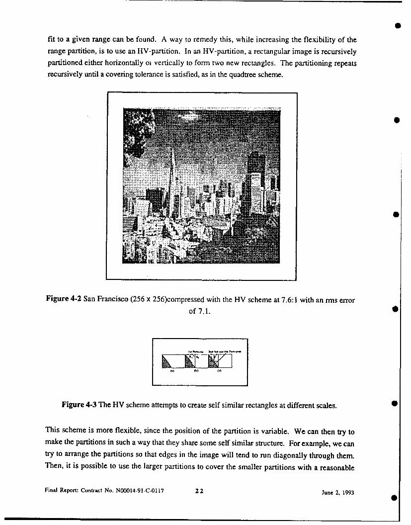
fit to a given range can be found. A way to remedy this, while increasing the flexibility of therange partition, is to use an HV-partition. In an HV-partition, a rectangular image is recursivelypartitioned either horizontally oi vertically to form two new rectangles. The partitioning repeatsrecursively until a covering tolerance is satisfied, as in the quadtree scheme.

Figure 4-2 San Francisco (256 x 256)compressed with the HV scheme at 7.6:1 with an rms error

of 7.1. 0

Figure 4-3 The HV scheme attempts to create self similar rectangles at different scales. S

This scheme is more flexible, since the position of the partition is variable. We can then try tomake the partitions in such a way that they share some self similar structure. For example, we cantry to arrange the partitions so that edges in the image will tend to run diagonally through them.Then, it is possible to use the larger partitions to cover the smaller partitions with a reasonable


| II mm

expectation of a good cover. Figure 4-3 demonstrates this idea. The figure shows a part of animage (a); in (b) the first partition generates two rectangles, RI with the edge running diagonally

through it, and R2 with no edge; and in (c) the next three partitions of RI partition it into 4rectangles, two rectangles which can be well covered by R, (since they have an edge runningdiagonally) and two which can be covered by R2 (since they contain no edge). Figure 4-2 showsan image of San Francisco encoded using this scheme.

Triangular Partitioning

A third way to partition an image is based on triangles. In the triangular partitioning scheme, arectangular image is divided diagonally into two triangles. Each of these is recursively subdivided

into 4 triangles by segmenting the triangle along lines that joia three partitioning points along thethree sides of the triangle. This scheme has several potential advantages over the HV-partitioningscheme. It is flexible, so that triangles in the scheme can be chosen to share self-similar properties,as before. The artifacts arising from the covering do not run horizontally and vertically, and this isless distracting. Also, the triangles can have any orientation, so we break away from the rigid 90

degree rotations of the quadtree and HV partitioning schemes. This scheme, however, remains to

be fully developed and explored.

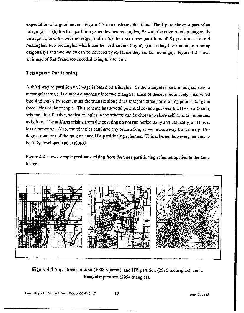
Figure 4-4 shows sample partitions arising from the three partitioning schemes applied to the Lena

image.

Figure 4-4 A quadtree partition (5008 squares), and HV partition (2910 rectangles), and a

triangular partition (2954 triangles).


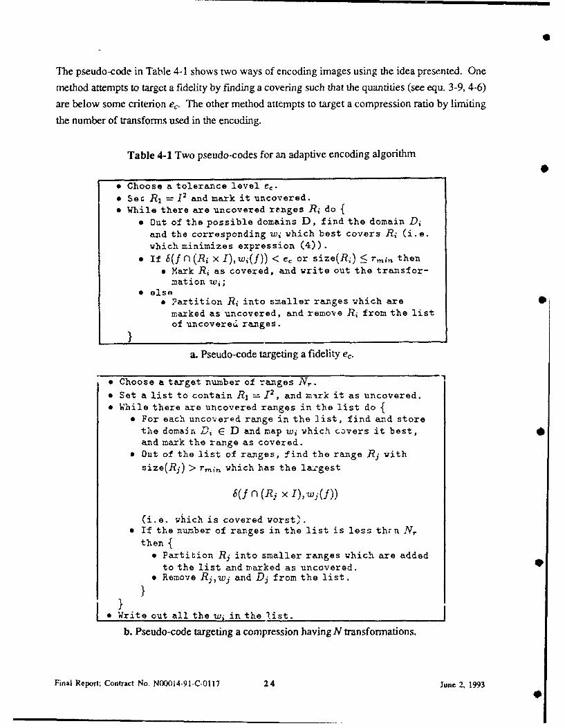
The pseudo-code in Table 4-1 shows two ways of encoding images using the idea presented. One

method attempts to target a fidelity by finding a covering such that the quantities (see equ. 3-9, 4-6)

are below some criterion e, The other method attempts to target a compression ratio by limiting

the number of transforms used in the encoding.

Table 4-1 Two pseudo-codes for an adaptive encoding algorithm

"* Choose a tolerance level e,."* Sec R, = 12 and mark it uncovered."* While there are uncovered renges Ri do {

"* Out of the possible domains D, find the domain Diand the corresponding wi which best covers Rj (i.e.which minimizes expression (4)).

"* If b(f n (Ri x I), w 1(f)) < e, or size(R;) < r then* Mark Ri as covered, and write out the transfor-

mation wi1 ;"* else

e Partition Ri into smaller ranges which aremarked as uncovered, and remove Ri from the listof uncovered ranges.

a. Pseudo-code targeting a fidelity e,

• Choose a target number of -ranges N,.* Set a list to contain R1 = J2, and mark it as uncovered.• While there are uncovered ranges in the list do {

"* For each uncovered range in the list, find and storethe domain Di E D and map wi which covers it best,and mark the range as covered.

"* Out of the list of ranges, find the range Rj with

size(Ri) > rmij which has the la•cgest

b~ n (Rj x1) (

(i.e. which is covered worst)."* If the number of ranges in the list is less thrn N,.

then {"* Partition Rj into smaller ranges which are added

to the list and marked as uncovered. 9"* Remove Rj,wj and Dj from the list.I

Write out all the wi in the 1ist.

b. Pseudo-code targeting a compression having N transformations.


4.3.1.2 Storing the Encoding Compactly

To store the encoding compactly, we do not store all the coefficients in equation (4-'. Thecontrast and brightness settings are stored using a fixed number of bits. One could compute the

optimal si and oi and then discretize them for storage. However, a significant improvement infidelity can be obtained if only discretized si and oi values are used when computing the errorduring encoding. Using 5 bits to store si and 7 bits to store oi has been found empirically optimal

* in general. The distribution of si and oi shows some structure, so further compression can beattained by using entropy encoding.

The remaining coefficients are computed when the image is decoded. In their place we store Riand Di. In the case of a quadtree partition, Ri can be encoded by the storage order of thetransformations if we know the size of Ri. The domains Di must be stored as a position and size(and orientation if diagonal domains are used). This is not sufficient, though since there are 8ways to map the four corners of Di to the corners of Ri. So we also must use 3 bits to determine

* this rotation and flip information.

In the case of the HV-paiitioning -d triangular partitioning, the partitions stored as a collection ofoffset values. As the rectangles (or triangles) become smaller in the partition, fewer bits arerequired to store the offset value. The partition can be completely reconstructed by the decodingroutine. One bit must be used to determine if a partition is further subdivided or will be used as anRi and a variable number of bits must be used to specify the index of each Di in a list of all thepartitions. For all three methods, and without too much effort, it is possible to achieve acompression of roughly 31 bits per wi on average.

The partitioning algorithms described are adaptive in the sense that they utilize a range size whichvaries depending on the local image complexity. For a fixed image, more transformations lead tobetter fidelity but worse compression. This trade-off between compression and fidelity leads to

two different approaches to encoding an image f - one targeting fidelity and one targetingcompression. These approaches are outlined in the pseudo-code in table 4-1. In the table, size(RA) refers to the size of the range; in the case of rectangles, size (Ri) is the length of the longest

side.

The images in Appendix 2 show typical results for our HV partitioning scheme.

Final Report: Contract No. N00014-91-C.0117 25 Jv'ne 2, 1993

4.3.1.3 Improving Encoding Speed

Our encoding algorithm consists of searching through a large number of sub-images, in order to

find one which has a low RMS error when correlated with a piece of a quadtree partition of theimage. In order to reduce this search time, we classify the collections of sub-images. The search

is limited to elements of the same class, leading to a reduced search time.

Our classification is as follows:

Each sub-image is first partitioned into 4 equal quadrants, which are ordered by brightness.This ordering leads to 3 classes, once a rotation and a reflection are used to bring thebrightest quadrant into the upper left position. This gives three classes and also determines

a rotation (reducing the search class by a factor of 4 or 8, the number of symmetryoperations on the square or rectangle respectively.

These three classes are further split into 12 or 24 by ordering the contrast levels of the sub-

quadrants of each quadrant. This gives a total of 36 or 72 classes.

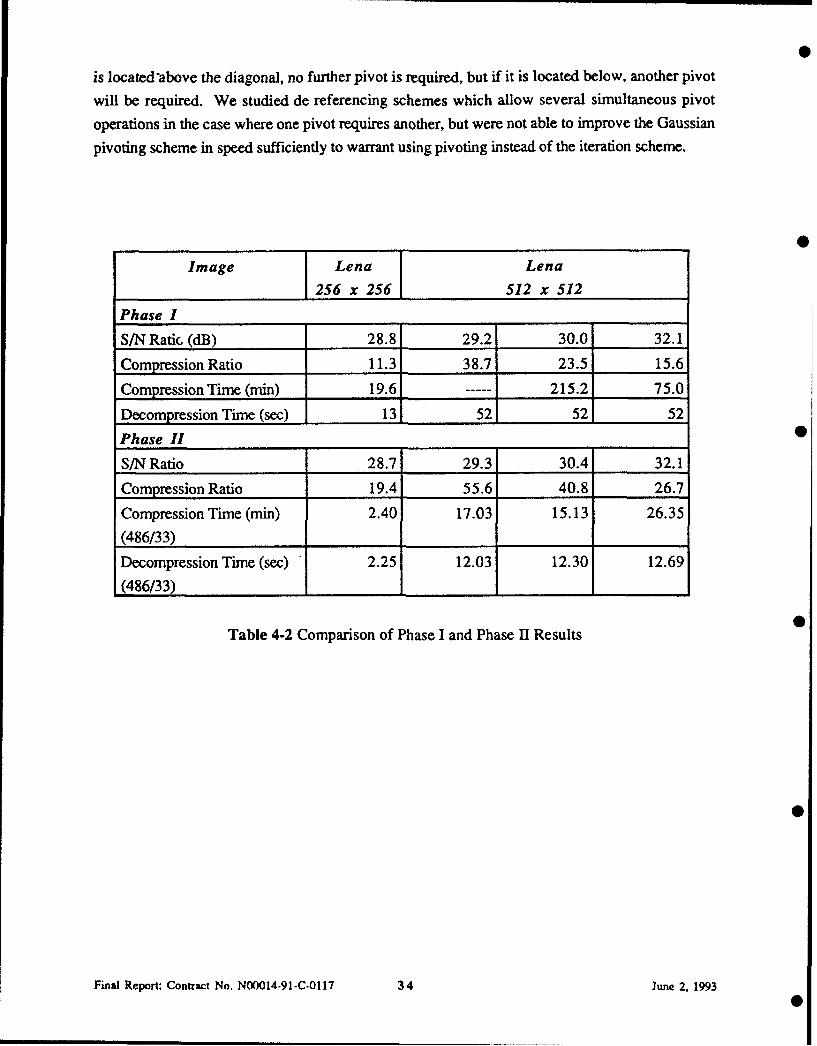
We were able to achieve a 15-fold increase in encoding speeds. Typical times for an Intel 80486-

33 are given in Table 4-2. Phase I time values are approximate due to a change in the development

platform.

4.3.1.4 Optical Methods

In anticipation of future developments in optical processing, we investigated the feasibility ofperforming tile comparisons optically. This was carried out in collaboration with Foster-Miller.

The method we investigated was optical four wave mixing.

Optical four wave mixing can be used to construct the convolution correlation of four images. This

operation may be represented by

Ir = 1]1 (12 * 13), (4-12)

where rI, 11, 12, and 13 denote the output and the three input images respectively, while

represents the correlation operation and * represents the convolution operation.


L tI

The major bottleneck in computing an IFS code for an image is checking the large set of possible

linear transforms and windows. In particular, it is necessary to compute

lw= T (W . I) * 1, (4-13)

for a large number of linear transforms, T, and windows, W. In this formula, • represents

multiplication while * represents correlation. In particular W - I is the windowed image

corresponding to a tile Ri in some partition above.

In order to put this into the form of a three wave product we use the convolution theorem:

W • I = F1 (FW * FI), (4-14)

where F and F -1 correspond to the Fourier transform and inverse Fourier transform respectively.

Applying Formula (4-14) to Formula (4-13) we obtain

IW = TF-1 (FW*FI) * I. (4-15)

The composition of operators TF -1 can also be written F -1 TF, where TF is the linear transform

induced by T in the spatial frequency domain.

The operation described by Equation (4-15) was implemented by means of optical techniques by a

group under Larry Domash of Foster Miller [26] and [27). Figure 4-5, supplied by Dr. Domash's

* group, shows a test case based on the Spierpinsky triangle.

We also modeled the optical process described above by means of the FFT. To do this, we

developed an FFT code for comparing domain and range tiles. The FF1 replaces a large portion of

the innermost loop of our present code. In essence, the code replaces repeated computation of

cross correlations by a single computation, based on the convolution property of the Fourier

transform. By taking advantage of the fact that one of the inputs to the convolution computation is

mostly zero and the fact that the FFT of the image need only be computed once, we can reduce the

convolution to one FFT per domain tile. Our benchmark studies indicated that optical methods

would give a considerable speedup of the compression algorithm, but unfortunately optical

methods do not presently yield the accuracies we require.


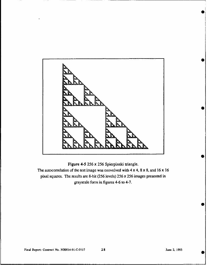
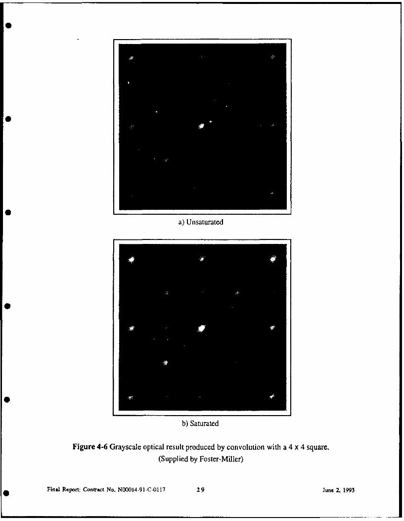
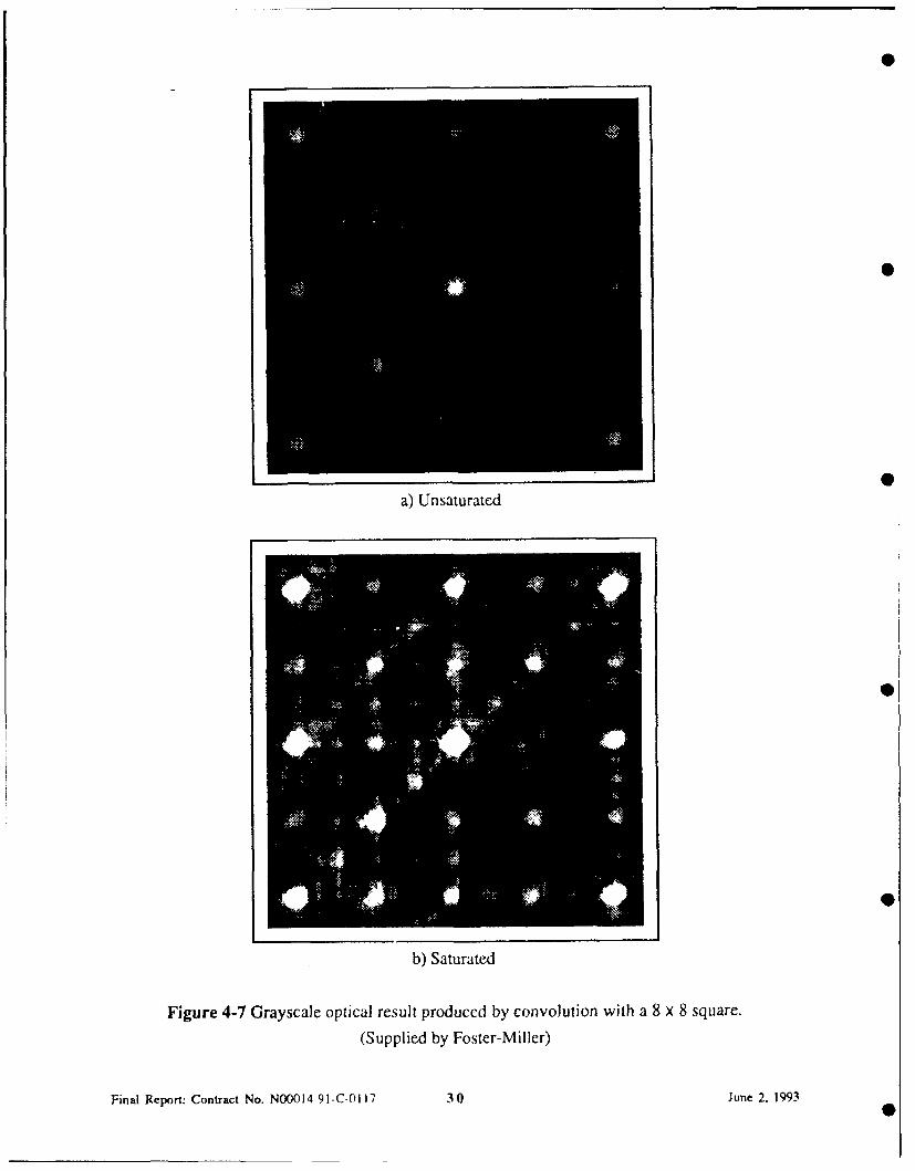
Figure 4-5 256 x 256 Spierpinski triangle.The autocorrelation of the test image was convolved with 4 x 4, 8 x 8, and 16 X 16

pixel squares. The results are 8-bit (256 levels) 256 x 256 images presented ingrayscale form in figures 4-6 to 4-7.


a) Unsaturated

b) Saturated


(Supplied by Foster-Miller)


a) Unsaturated

b) Saturated



Final Report: ContTact No. N00014-91-C-0117 30 June 2, 1993

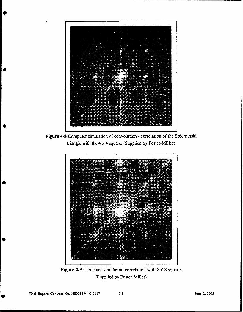
Figure 4-8 Computer simulation of convolution - correlation of the Spierpinski

triangle with the 4 x 4 square. (Supplied by Foster-Miller)

Figure 4-9 Computer simulation-correlation with 8 x 8 square.



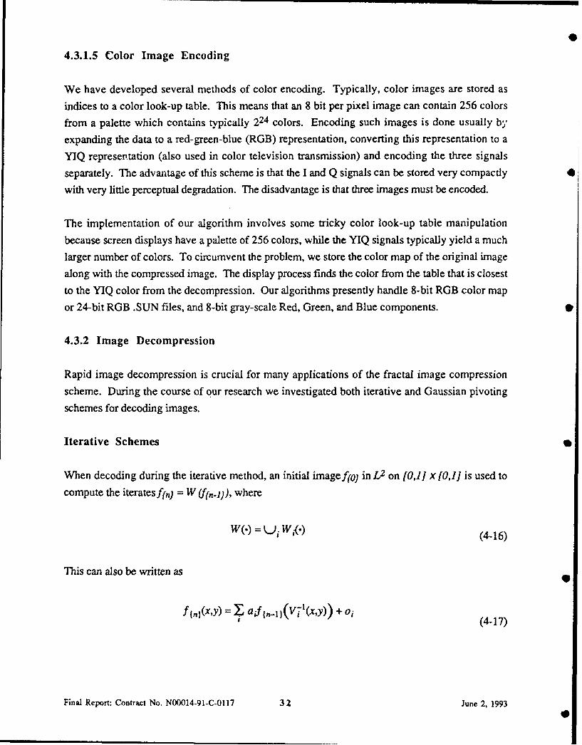
4.3.1.5 Color Image Encoding

We have developed several methods of color encoding. Typically, color images are stored as

indices to a color look-up table. This means that an 8 bit per pixel image can contain 256 colors

from a palette which contains typically 224 colors. Encoding such images is done usually by

expanding the data to a red-green-blue (RGB) representation, converting this representation to a

YIQ representation (also used in color television transmission) and encoding the three signals

separately. The advantage of this scheme is that the I and Q signals can be stored very compactly

with very little perceptual degradation. The disadvantage is that three images must be encoded.

The implementation of our algorithm involves some tricky color look-up table manipulation

because screen displays have a palette of 256 colors, while the YIQ signals typically yield a much

larger number of colors. To circumvent the problem, we store the color map of the original image

along with the compressed image. The display process finds the color from the table that is closest

to the YIQ color from the decompression. Our algorithms presently handle 8-bit RGB color map

or 24-bit RGB .SUN files, and 8-bit gray-scale Red, Green, and Blue components.

4.3.2 Image Decompression

Rapid image decompression is crucial for many applications of the fractal image compression

scheme. During the course of our research we investigated both iterative and Gaussian pivoting

schemes for decoding images.

Iterative Schemes

When decoding during the iterative method, an initial imagef{o) in L2 on [0,11 X [0,11 is used to

compute the iteratesf{n) = W (f[n-1)), where

W(.) = '.Ji W,(.) (4-16)

This can also be written as

f 1 ,,(x,y) = jZ aif1 l.i(VT'(x,y)) + oiC J(4-17)

Final Report: Contract No. N00014-91-C-0117 3 2 June 2, 1993

where thi ith term of the summation is defined on the region Ri, Vi is an affine transformation on

the region Ri, and ai and oi are contrast and intensity adjustments respectively.

We implemented integer versions of the iteration scheme with a variant on the storage of the

transforms. In the iterative scheme, each pixel depends upon another (with a brightness and a

contrast adjustment). Rather than computing this dependency from the transformations at each

iteration step, we compute it initially. This also appears to lead to considerable improvement in

0 decoding times. The final version of our algorithm handles color, smoothing to eliminate artifacts,

and sampling or averaging of domain pixels onto the range pixels.

Gaussian Pivoting

Suppose we are decompressing an image of M xM pixels. We can write the image as a columnvector, and then the above equation can be written.

f~n] = Sfin-1) + 0 (4-18)

where S is an M2 xM2 matrix with entries sjy which encode the contrast adjustments ai and spatial

affine transformations Vi and 0 is a column vector encoding the intensity adjustments. Then

n-1fm= =5flf 0 ) + SO (4-19)

If each sij is less than 1 then the first term is 0 in the limit. This condition can be relaxed if W is

eventually contractive. When I - S is invertible

f=, sio = (I - S)-0 (4-20)

If each pixel value off(n) depends upon only one (or even a few) pixel values off{n-l) then I - S isvery sparse and is inverted readily by sparse matrix methods. We have implemented this algorithm

and it shows promising results. It runs considerably faster than the previous version of theiteration algorithm.

We developed a decoding algorithm which triangularizes the S matrix by pivoting. We have

observed that different pivoting schemes lead to different decoding times since each pivot operation

eliminates an entry in one place in the matrix and creates another somewhere else. If the new entry


is located-above the diagonal, no further pivot is required, but if it is located below, another pivot

will be required. We studied de referencing schemes which allow several simultaneous pivot

operations in the case where one pivot requires another, but were not able to improve the Gaussian

pivoting scheme in speed sufficiently to warrant using pivoting instead of the iteration scheme.

Image Lena Lena

1256 x 256 512 x 512

Phase I

S/N Ratio (dB) 28.8 29.2 30.0 32.1

Compression Ratio 11.3 38.7 23.5 15.6

Compression Time (min) 19.6 215.2 75.0

Decompression Time (sec) 13 52 52 52

Phase II 0

S/N Ratio 28.7 29.3 30.4 32.1

Compression Ratio 19.4 55.6 40.8 26.7

Compression Time (min) 2.40 17.03 15.13 26.35

(486/33)

Decompression Time (sce) 2.25 12.03 12.30 12.69

(486/33)

0

Table 4-2 Comparison of Phase I and Phase II Results


*

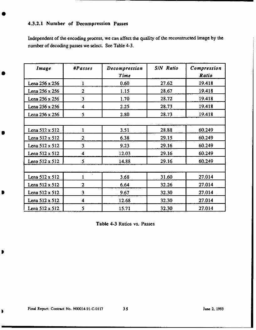
4.3.2.1 Number of Decompression Passes

Independent of the encoding process, we can affect the quality of the reconstructed image by the

number of decoding passes we select. See Table 4-3.

Image #Passes Decompression SIN Ratio Compression

Time Ratio

Lena 256 x 256 1 0.60 27.62 19.418

Lena 256 x 256 2 1.15 28.67 19.418

Lena 256 x 256 3 1.70 28.72 19.418

Lena 256 x 256 4 2.25 28.73 19.418

Lena 256 x 256 5 2.80 28.73 19.418

Lena 512 x 512 1 3.51 28.88 60.249

Lena 512 x 512 2 6.38 29.15 60.249

Lena 512 x 512 3 9.23 29.16 60.249

Lena 512 x 512 4 12.03 29.16 60.249

Lena 512 x 512 5 14.88 29.16 60.249

Lena 512 x 512 1 3.68 31.60 27.014

Lena 512 x 512 2 6.64 32.26 27.014

Lena 512 x 512 3 9.67 32.30 27.014

Lena 512 x 512 4 12.68 32.30 27.014

Lena 512 x 512 5 15.71 32.30 27.014

Table 4-3 Ratios vs. Passes


5.0 WaVelet Image Compression

5.1 Background

Because the fractal compression method has not been entirely satisfactory for some types of images

such as maps, fingerprints and satellite images we have implemented a version of the wavelet

compression method reported by Antonini [1].

This encoding method has three main steps: a wavelet transform followed by a lattice vector

quantization followed by a Huffman encoding of the output vectors. The Huffman code step is not

reported in the report by Antonini [1]. A standard codebook may be used for transmission, with a

provision for sending codebook entries for rarely-encountered vectors.

5.1.1 One Dimensional Wavelets

Wavelets are functions generated from one single function 4' by deletions and translations

ya,,(x) = IaI' V(x (5-1)

Generally we require that the metric wavelet 41 should be well localized in time and frequency and

have zero mean.

The basic idea of the wavelet transform is to represent any arbitrary function f as a superposition

of wavelets. For example we may write

f(x) = f dadb c(a,b) /Vabj,(X) (5-2)

In practice we deal with discrete decompositions

0

fZ Cmnfa~b (5-3)

Where /fmsn(x) = 2-'h (2-mx - n) (5-4)

Final Report: .Zontract No. N00014-91-C-0117 36 June 2, 1993

is the dual basis to *m.n and

c, ( VmJ) - f V,,,(x)f(x) dr (5-5)

The basic wavelet is constructed from a scaling function qo such that

fp(x) = aqV(2x- k) (5-6)

such that

f V(x) -x= (5-7)

and O(x) is given by

W/(x) = (-l)' cc,.,•p(2x + k)k (5-8)

The quantities crk are the wavelet coefficients. In order to measure orthagonality we require that

a,+,-=2-' i= -1,2

Sacxk+2,= {2if1i=0 (5-9)A:. Oifl•0

5.1.2 Quadrature Mirror Filters

The wavelet coefficients define a low pass filter sequence. Following the notation of Beylkin, et al

[4] we write the conditions

(1) I. Ih,4 I./1h < -o for somee (5-10)

(2) Zh~j÷,= 21h i=0,1 (5-11)


(3) • ~•z ,(5-12)

Note that the h's r.'place the -'s above. Let g = WgJ be defined by gj = (-1)/ hi-. Then (h,g] is a

pair of quadrature muiror filters and we can define two operations H and G. For any function f,

Hf(x) = hj (2x- J()j ~(5-13)

Gf(x) = g gf(2x (514j (5-14)

If the sequences g, h are fialte we can define p = lim ,mHn(x) where X is the indicator

function of [- 1/2,1/2]. Note that p is the unique fixed function of the equation (P = HP.

Furthermore G and H have adjoints

H~~x hjf(I + (-5

G*f(x) =½ gjf (X + j)(-62 + (5-16)

We have the identities HHX=GG*=I, HG*=GH*= 0 and H*H+G*G=I. These identities can be

used in the construction of multiresolution pyramids (as in Mallat [20] or Beylkin, et al [4]).

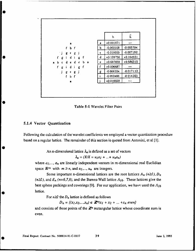
5.1.3 Multidimensional Analysis

Our research is based on the non-separable and non-oriented filters described by Antonini, et al[1]. We decompose images with a multiresolution scale factor q12. The scaling function is defined

via

,,n = 2'' 0 (L2m(x,y) - n) n = (nXny) (5-17)

This translates into a pair of filters as given in Table 5-1.


h

a a +0.001671 -

f b f b -0.002108 -0.005704

j g c g j c -0.019555 -0.007192

f g i d i g f d +0.139756 +0.164931

a b c d e d c b a e .0.687859 +0.586315

f g i d i g f f .0.006687 -

j g C g j -0.006324 -0.017113

f b f i -0052486 -0.014385

a +0.010030 -

Table 5-1 Wavelet Filter Pairs

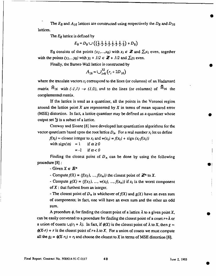
5.1.4 Vector Quantization

Following the calculation of the'wavelet coefficients we employed a vector quantization procedure

based on a regular lattice. The remainder of this section is quoted from Antonini, et al [1].

An n-dimensional lattice A, is defined as a set of vectors

4 = (XIX = uial + ... + uan)

where al,..., an are linearly independent vectors in m-dimensional real Euclidian

space Rm with m Ži n, and ul,..., un are integers.

Some important n-dimensional lattices are the root lattices An (nŽ1), Dn

(n>2), and En (n=6,7,8), and the Barnes-Wall lattice A16 . These lattices give the

best sphere packings and coverings [9]. For our application, we have used the A16

lattice.

For nŽ2 the D, lattice is defined as follows

Dn = ((xl,x2,...,xn) IE Z"/xj + X2 + ... +xn even)

and consists of those points of the Z" rectangular lattice whose coordinate sum is

even.


The E8 and A16 lattices are constructed using respectively the D8 and D16

lattices.The E8 lattice is defined by

Es = DsU((½.U. .04 744 ) + DQ

E8 consists of the points (xj,...,x8) with xi E Z and ,xi even, togetherwith the points (yj,...yS) with yi + 1/2 e Z + 1/2 and ,jyi even.

Finally, the Barnes-Wall lattice is constructed by

A 16 U=' - (ri + 2D16)

where the translate vectors ri correspond to the lines (or columns) of an Hadamard

matrix 116 with (-1,1) -- (1,0), and to the lines (or columns) of •16 the

complemented matrix.If the lattice is used as a quantizer, all the points in the Voronoi region

around the lattice point X are represented by X in terms of mean squared error(MSE) distortion. In fact, a lattice quantizer may be defined as a quantizer whose

output set 2J is a subset of a lattice.

Conway and Sloane [8] have developed last quantization algorithms for thevector quantizers based upon the root lattice Dn. For a real number xi let us define

f(xi) = closest integer to xi and w(xi) = f&x,) + sign (x-if(xi))with sign(a) =1 if a_0

=-I ifa<0

Finding the closest point of Dn can be done by using the following

procedure [8] : 0

- Given Xe Rn

- Computef(X) = (fxj), ..., f(xn)) the closest point of Zn to X.

- Compute g(X) = (f(x]), ..., w(x), .... ,f(xn)) if xi is the worst component

ofX : that furthest from an integer.

- The closest point of Dn is whichever of f(X) and g(X) have an even sumof components; in fact, one will have an even sum and the other an odd

sum.

A procedure 4, for finding the closest point of a lattice X to a given point X,

can be easily converted to a procedure for finding the closest point of a coset r+A ora union of cosets •i(ri + A). In fact, if O(X) is the closest point of A to X, then g =O(X-r) + r is the closest point of r+2 to X. For a union of cosets we must computeall the gi = •(X-ri) + ri and choose the closest to X in terms of MSE distortion [8].


Since E8 is the union of two cosets of D8 , and AM6 is the union of 32 cosets

of D16 , then we can use the previous encoding procedure to find the closest point of

E8 or A 6 to X.

5.1.5 Huffman Encoding

We implemented a Huffman coding algorithm to compress the quantized coefficients of the wavelet

decomposition. This well-known scheme assigns short code words to the most probable input

symbols and longer code words to the least probable ones to obtain an encoding with a small

average code length.

The input symbols to the Huffman encoder are quantized wavelet coefficients within 4 x 4 blocks,i.e. vectors of 16 elements, in the coefficient domain. The procedure below converts a list of the

frequencies for each unique input symbol into a binary tree which provides the code for each of the

input symbols. Each element in the frequencies list represents either a unique symbol or the sum of

the frequencies of a subset of the unique symbols.

1: Search the list of frequencies for the two elements with the lowest frequencies.

2: Replace these two elements with their sum. The updated list has one less element.

Both of the replaced elements will have Huffman codes one bit longer than their sum will

have.

3: Go back to step 1 and repeat the procedure until the list contains only one element.

The external nodes of the tree represent the different vectors V1, V2, V3, ... We interpret a '0' as

a left branch and a T as a right branch and get the Huffman codes for the vectors V 1, V2, V3,

respectively.

A concise description of the Huffman coding algorithm can be found in [15] and (23].

In our system, we limit the length of any Huffman code to 15 bits since:

a) This is long enough for most images.

b) For any image requiring longer Huffman codes the compression ratio is not good.


5.1.5.1 Adaptive Huffman-Coding For Code Book Generation

An arbitrary set of images, the training set, is processed as above to generate a standard code book.

The input symbols occurring with higher frequency in these images are assigned shorter codes. A

number of longer codes are fixed in advance for new symbols which will occur in other images,

the testing set. Here, we assume that most symbols in the testing images can be found in the

standard code book and only a few symbols need to be treated as new.

The compression ratios resulting from this code book approach are dependent on the symbols

selected from the training set. Any uncommon symbols in the code book will lengthen the codes

for all the new codes. The number of symbols in a training set of ten images ranges from 1100 to

3100 depending on the system scale factor (factorK) and the particular images. The number of

new symbols may range from 2500 to 8000 depending on the referent code book. This system

only handles those images which present fewer new symbols than the number of codes available in

the code book.

5.2 Approach

Figure 5-1 is a block diagram of the system. In addition to the provision for sending vectors not in

the codebook we have included the capability of sending error bits which give additional significant

bits to correct the output of the vector quantization.

The wavelet transform step may use either separable or non separable filters. As in Antonini's S

report, we have implemented a version of the quincunx pyramid for the non separable case. Thesefilters produce a decomposition with a multi-resolution scale factor of •42. Other non-separable

filters are also possible, as reported by Lawton and Resnikov [19] and Gr6chenig and Madych

[14] but have not yet been investigated. One curious aspect of some of these filters is that the

domain of support of the associated wavelet is a set with a fractal boundary, which can be used to

give a periodic tiling of the plane.

In our present system we perform levels of transform in the quincunx pyramid. This replaces the S

original image by a set of "super blocks" of wavelet coefficients of different types. Because six

levels are performed this gives 256 types of coefficients each type corresponding to a different

series H to G operations (as identified in the background section). For example, one set of

coefficients would correspond to HHHHHHHH and a second to HHHHHHHG a third to

HHHHHHGH and so forth.


This has the effect of replacing an original 512 x 512 image by 4096 blocks of 64 coefficients

each. I.E. there are 4096 coefficients of a given type. Statistical analysis of the various types of

coefficients indicates that most of the original image intensity will be concentrated in a few types of

coefficients, one of which is the coefficient arising from the HHHHHHHH operation. The

statistical variation is correspondingly greater of the coefficients which concentrates the image

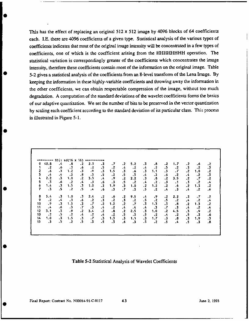
intensity, therefore these coefficients contain most of the information on the original image. Table

5-2 gives a statistical analysis of the coefficients from an 8-level transform of the Lena Image. By

keeping the information in these highly-variable coefficients and throwing away the information in

the other coefficients, we can obtain respectable compression of the image, without too much

degradation. A computation of the standard deviations of the wavelet coefficients forms the basics

of our adaptive quantization. We set the number of bits to be preserved in the vector quantization

by scaling each coefficient according to the standard deviation of its particular class. This process

is illustrated in Figure 5-1.

SOj: sd(16 x 16)0 40.8 .4 .8 .2 2.3 .3 .7 .2 5.2 .3 .8 .2 1.7 .2 .6 .21 .2 .6 .3 .6 .2 .5 .2 .4 .2 .4 .2 .5 .2 .3 .2 .32 .6 .3 1.2 .3 .9 .3 1.5 .3 .6 .3 1.1 .3 .7 .2 1.0 .23 .4 .4 .3 .8 .3 .5 .2 .5 .3 .4 .3 .6 .2 .4 .2 .34 2.2 .3 1.0 .2 3.3 .4 .9 .2 2.2 .3 .8 .2 3.5 .2 .7 .25 .3 .6 .2 .4 .3 .6 .3 .5 .2 .4 .2 .3 .1 .3 .2 .46 1.4 .3 1.5 .3 1.0 .3 1.9 .3 1.0 .2 1.2 .2 .6 .2 1.3 .27 .3 .5 .2 .5 .4 .6 .3 .7 .3 .5 .2 .4 .3 .4 .2 .6

8 5.4 .3 1.0 .3 2.4 .2 .6 .2 9.5 .4 .9 .2 2.2 .3 .7 .29 .2 .4 .3 .6 .2 .3 .2 .3 .2 .5 .2 .5 .2 .4 .2 .4.

10 .9 .3 1.5 .3 .7 .2 1.2 .2 .7 .3 1.3 .3 .8 .2 1.3 .211 .4 .6 .3 .7 .3 .4 .2 .4 .4 .4 .3 .7 .3 .4 .2 .412 3.1 .3 .9 .2 3.4 .Z .8 .2 2.5 .3 1.0 .2 4.5 .3 .9 .213 .2 .5 .2 .4 .2 .4 .2 .5 .3 .5 .2 .4 .2 .5 .3 .614 1.0 .3 1.5 .3 .7 .3 1.3 .3 1.1 .3 1.7 .3 .8 .3 1.9 .315 .3 .5 .2 .5 .3 .5 .3 .6 .3 .5 .2 .5 .4 .5 .3 .8

Table 5-2 Statistical Analysis of Wavelet Coefficients


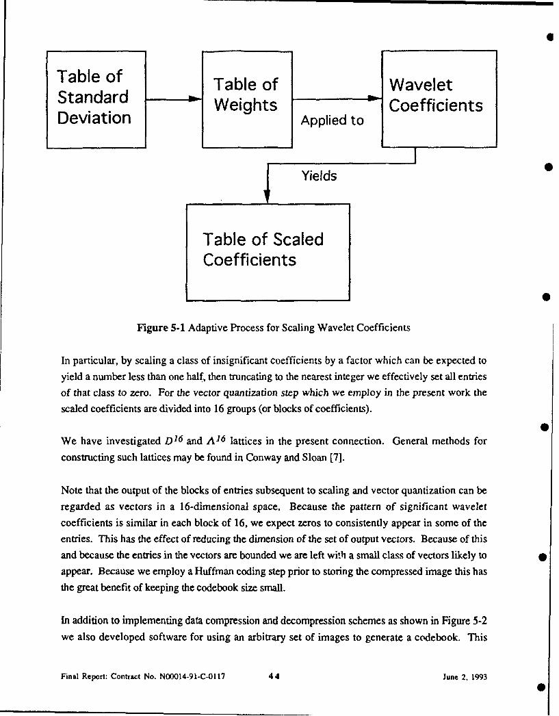
Table of Table of WaveletStandard T of W e

Deviation Weights Applied to Coefficients

SYields

Table of ScaledCoefficients

Figure 5-1 Adaptive Process for Scaling Wavelet Coefficients

In particular, by scaling a class of insignificant coefficients by a factor which can be expected to

yield a number less than one half, then truncating to the nearest integer we effectively set all entries

of that class to zero. For the vector quantization step which we employ in the present work the

scaled coefficients are divided into 16 groups (or blocks of coefficients).

We have investigated D 16 and A 16 lattices in the present connection. General methods for

constructing such lattices may be found in Conway and Sloan [7].

Note that the output of the blocks of entries subsequent to scaling and vector quantization can be

regarded as vectors in a 16-dimensional space. Because the pattern of significant wavelet

coefficients is similar in each block of 16, we expect zeros to consistently appear in some of the

entries. This has the effect of reducing the dimension of the set of output vectors. Because of this

and because the entries in the vectors are bounded we are left with a small class of vectors likely to

appear. Because we employ a Huffman coding step prior to storing the compressed image this has

the great benefit of keeping the codebook size small.

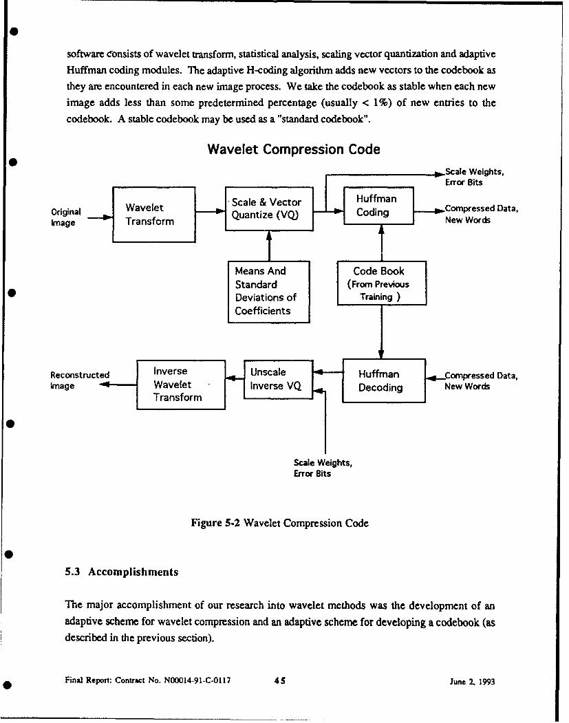
In addition to implementing data compression and decompression schemes as shown in Figure 5-2

we also developed software for using an arbitrary set of images to generate a codebook. This


0i

software consists of wavelet transform, statistical analysis, scaling vector quantization and adaptive

Huffman coding modules. The adaptive H-coding algorithm adds new vectors to the codebook asthey are encountered in each new image process. We take the codebook as stable when each new

image adds less than some predetermined percentage (usually < 1%) of new entries to the

codebook. A stable codebook may be used as a "standard codebook".

Wavelet Compression Code0

--Scale Weights,Scale & VectorBits

Original Wavelet Scale (Vor Hodin Compressed Data,Image Transform Quantize (VQ)Words

Means And Code BookStandard (From PreviousDeviations of Training)Coefficients

Reconstructed Inverse Unscale - Huffman .. Compressed Data,Image Wavelet Inverse VQ Decoding New Words

Transform

Scale Weights,Error Bits

Figure 5.2 Wavelet Compression Code

05.3 Accomplishments

The major accomplishment of our research into wavelet methods was the development of an

adaptive scheme for wavelet compression and an adaptive scheme for developing a codebook (asdescribed in the previous section).


Up to the present, our investigations have been limited to a selection of 128 x 128 and 512 x 512

greyscale images, but the results are promising. A typical compression run on both sizes of

images produces a 12:1 compression ratio or better at a 30 dB peak signal-to-noise ratio. Thevisual quality of some types of reconstructed images is very good; in fact the error image must be

scaled up to be visible on our computer screen under ambient light. Good image quality waspreserved for both faces and fingerprints at the 12:1 compression ratio. Typical times for encoding

a 128 x 128 image are about 5 minutes and decoding about 3 minutes on a 486 processor. We 0have not yet attempted to optimize Lhe code.

Figures 8 and 9 in Appendix 2 show images of a fingerprint compressed and decompressed by

means of our wavelet code. Note that the artifacts in the decompressed images are much less

apparent than the artifacts in images reconstructed from the fractal code. These figures also showfingerprints coded and reconstructed by means of fractal techniques. Note that the artifacts in thefractal reconstruction appear to be "blocky", while the artifacts in the wavelet reconstruction appear

to be induced by edge effects. 0

6.0 Conclusions

NETROLOGIC's work in image compression resulted into two complete software programs for

the PC environment where both fractals and wavelets were successfully employed. Each approachhas subsets of images where advantages accrue. In general wavelets can provide better quality athigh compression ratios, but fractals enable fast and simple decompression. S

6.1 Potential Dual-Use Follow On

NETROLOGIC has entered a joint venture with CST Images to implement the wavelet code

developed in this program with an 1860 accelerator board. In addition, we received a request to

use our techniques to compress a movie segment and are setting up a CRDA with NRD in San

Diego. We entered discussions with a major oil company to apply our compression methods to

compression seismic logs which currently occupy 100,000 magnetic tapes. 0


0

Referen-ces

[1] M. Antonini, M. Barlaud and P. Mathieu, "Image Coding Using Vector Quantization ofWavelet Coefficients", Proc. IEEE Int Conf. ASSP, Toronto Canada, 2273, May (1991).

[2] M. Barnsley and A. D. Sloan, "A Better Way to Compress Images", Byte, January (1988).

[3] M. Barnsley, Fractals Everywhere, Academic Press, San Diego, (1989).

[4] G. Beylkin, R. Coifman and V. Rokhlin, "Fast Wavelet Transforms and Numerical

Algorithms", Comm. Pure Appl. Math, 44:141-183 (1991)

[5] R.D. Boss and E.W. Jacobs, "Fractal-Based Image Compression", NOSC Technical Report1315, September 1989. Naval Ocean Systems Center, San Diego, CA 92152-5000.

[6] R.D. Boss and E.W. Jacobs, "Fractal-Based Image Compression II", NOSC Technical Report

1362, June 1990. Naval Ocean Systems Center, San Diego, CA 92152-5000.

[7] J. H. Conway and N. J. A. Sloane, "Voroni Regions of Lattices, Second Moments ofPolytopes and Quantization", IEEE Transactions on Information Theory, 28:211, (1982)

[8] J. H. Conway and N. J. A. Sloane, "Fast Quantizing and Decoding Algorithms for LatticeQuantizers and Codes", IEEE Transactions on Information Theory, IT-28(No. 2):227,

(1982).

[9] J.H. Conway and N.J.A. Sloane, Sphere Packings, Lattices and Groups, Springer-Verlag,

New York (1988)

[10] S. Demko, L. Hodges and B. Naylor, "Construction of Fractal Objects with Iterated Function

Systems", Computer Graphics, 19:271, (1988).

[11] Y. Fisher, E.W. Jacobs and R.D. Boss, "Fractal Image Compression Using Iterated

Transforms", to appear in Data Compression, J. Storer, Editor, Kluwer Academic

Publishers, Norwall, MA.


[12] Y. Fisher, E.W. Jacobs and R.D. Boss, "Fractal Image Compression Using Iterated

Transforms", NOSC Technical Report, Naval Ocean Systems Center, San Diego, CA92152-5000.

[13] Y. Fisher and A. Lawrence, "Fractal Image Compression for Mass Storage Applications",

SPIE Proceedings (Image Storage and Retrieval Systems), 1662:244, (1992).

[14] K. Gr'6chenig and W. R. Madych, "Multiresolution Analysis, Haar Bases, and Self-SimilarTilings of Rne, IEEE Transactions on Information Theory, 38:556, (1992).

[15] E.L. Hall, Computer Image Processing and Recognition , Academic Press, New York

(1979).

[161 J. E. Hutchinson, "Fractals and Self Similarity", Indiana University Mathematics Journal,Vol.35, No.5, (1981).

[17] A. Jacquin, "A Fractal Theory of Iterated Markov Operators with Applications to DigitalImage Coding", Doctoral Thesis, Georgia Institute of Technology, (1989).

[18] E. W. Jacobs, Y. Fisher and R.D. Boss, "Image Compression: A Study of the IteratedTransform Method", to appear in Signal Processing.

[19] W. M. Lawton and H. L. Resnikoff, "Multidimensional Wavelet Bases", Preprint, Aware,Inc., Cambridge, Mass, (1991). S

[20] S. Mallat, "Multiresolution Approximation and Wavelets", Trans. Amer. Math. Soc.,

315:69-88 (1989)

[21] H. 0. Pietgen and D. Saupe, Editors, The Science of Fractals, Springer Verlag, New York

(1989).

[22] H. 0. Pietgen, D. Saupe and H. Jurgens, Editors, Fractalsfor Class Room, Springer Verlag, 0New York (1991).

[23] A. Rosenfeld and A. C. Kak, Digital Picture Processing, Second Edition, Volume 1,

Academic Press, Florida (1982).


S

[24] W. Rudin, Real and Complex Analysis, McGraw Hill, New York. (1974).

[25] E. Walach and E. Karnin, "A Fractal Based Approach to Image Compression", Proceedings

of ICASSP, Tokyo (1986)

[26] L. Domash, "Optical Computer for Fractal Image Analysis", Navy Report No. NAV-0238-FM-9179-444, March (1991).

[27] V. Ryan, "Preliminary Results for Image Compression via Fractal Analysis", Foster-Miller(Preprint), June (1992).


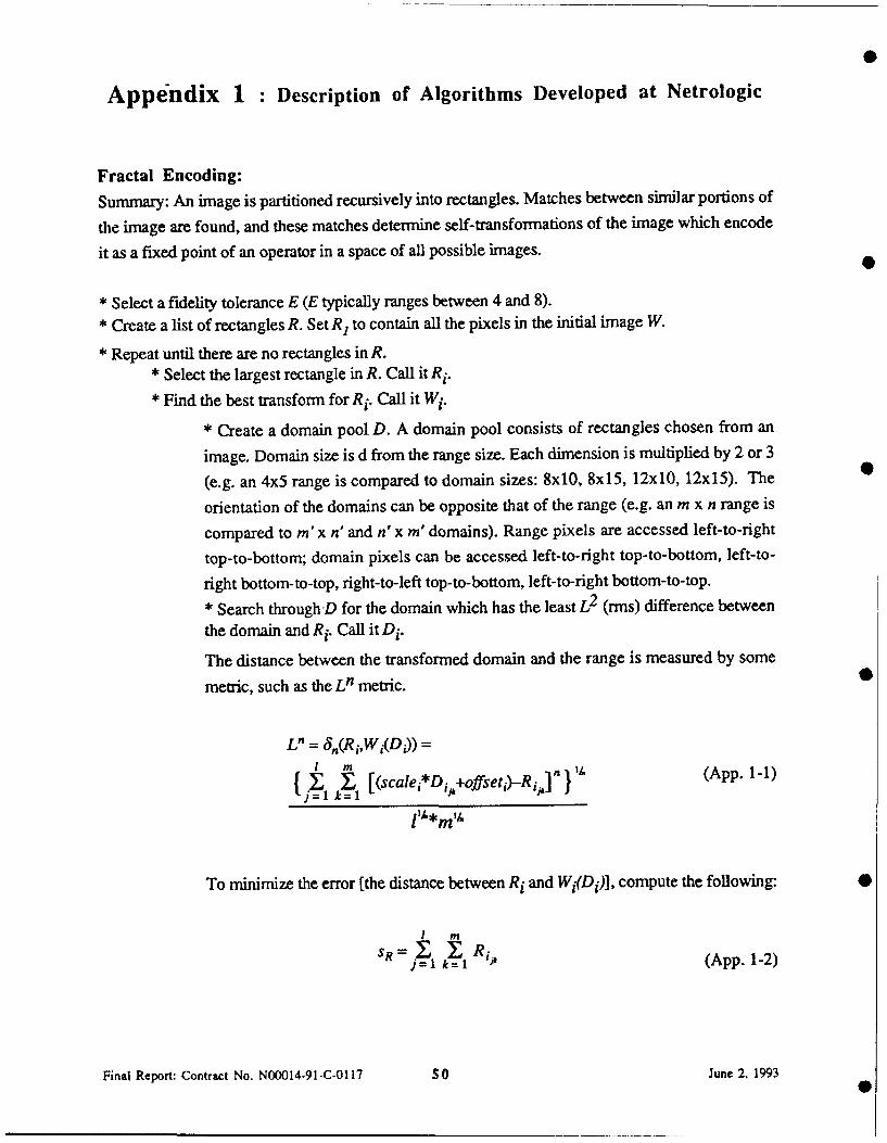
Appendix 1 : Description of Algorithms Developed at Netrologic

Fractal Encoding:

Summary: An image is partitioned recursively into rectangles. Matches between similar portions of

the image are found, and these matches determine self-transformations of the image which encode

it as a fixed point of an operator in a space of all possible images.

"* Select a fidelity tolerance E (E typically ranges between 4 and 8).

"* Create a list of rectangles R. Set R1 to contain all the pixels in the initial image W.

"* Repeat until there are no rectangles in R."* Select the largest rectangle in R. Call it Ri.

"* Find the best transform for Ri. Call it Wi.

* Create a domain pool D. A domain pool consists of rectangles chosen from an

image. Domain size is d from the range size. Each dimension is multiplied by 2 or 3

(e.g. an 4x5 range is compared to domain sizes: 8x10, 8x15, 12x10, 12x15). The -

orientation of the domains can be opposite that of the range (e.g. an m x n range is

compared to m' x n' and n' x m' domains). Range pixels are accessed left-to-right

top-to-bottom; domain pixels can be accessed left-to-right top-to-bottom, left-to-

right bottom-to-top, right-to-left top-to-bottom, left-to-right bottom-to-top.

* Search through-D for the domain which has the least L2 (rms) difference between

the domain and Ri. Call it Di.

The distance between the transformed domain and the range is measured by some

metric, such as the Ln metric.

L"= 3(RjWX(D)) =

{ n I [(scale*D- i (App. 1-1)

To minimize the error [the distance between Ri and Wi(Di)], compute the following: 0

1 M

SRj=1 k='R1 (App. 1-2)

Final Report: Contract No. N00014-91-C-0117 so June 2, 1993 0

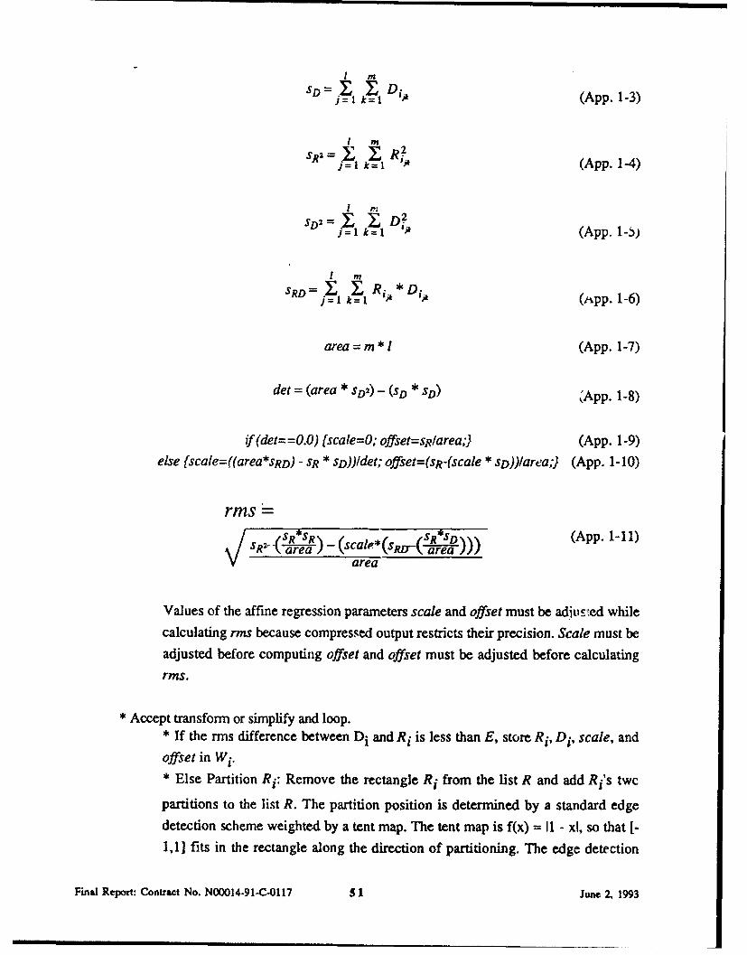
SD I D I

I m

J= 1 k 1 DA (App. 1-3)

j= I _ =1 (App. 1-4)

1 ft

SD=l T~l Dj (App. 1-a)

SRD --I Ri * Di1k= 1 ARi• (,,pp. 1-6)

area = m * I (App. 1-7)

det = (area * SD2) - (SD * SD) (App. 1-8)

if (det= =0.0) (scale=O; offset=su/area;) (App. 1-9)else (scale=((area*sRD) - SR * sD))Idet; offset=(sR-(scale * sD))/area;} (App. 1-10)

rms =

•a -re s al sR *S) (App. 1-11)• -• -S) t,•(- -)area

Values of the affine regression parameters scale and offset must be adjus ed whilecalculating rms because compressed output restricts their precision. Scale must beadjusted before computing offset and offset must be adjusted before calculating

rms.

• Accept transform or simplify and loop.* If the rms difference between Di and Ri is less than E, store Ri, Di, scale, and

offset in Wi.* Else Partition Ri: Remove the rectangle Ri from the list R and add Ri's twc

partitions to the list R. The partition position is determined by a standard edgedetection scheme weighted by a tent map. The tent map is f(x) = I1 - xl, so that [-1,1] fits in the rectangle along the direction of partitioning. The edge detection


scheme consists of finding the biggest absolute difference between successive row

or column sums.

* Output the list W with as much compression as possible.

Decoding:Summary: Decoding operates by iterating in the space of all images. Each transform Wi

determines how pixels in an image should map to other pixels in the image. Iterating these maps

converges to the fixed point image F.

* Read the list of transforms called W.

* Select a number of decoding steps N. N is image dependent. We have found that after 3

iterations there is no perceived improvement, thought the fixed point F rms continues 0o improve.

"* Create the fixed point image F. Its initial contents do not matter.

"* Repeat N times:

* Apply each transform Wi to F. The domain pixels are read from F, the range pixels are

written to F.

"* Output the image F.

References:

Y. Fisher, E.W. Jacobs, R.D. Boss, Iterated Transform Image Compression, NOSC Technical

Report 148, NOSC, San Diego, April (1991).

Y.F3her, -ractal Image Compression, Fractals and Chaos, H.O. Peitgen, D. Saupe, H.

Jurgens, Appendix A, Springer Verlag, New York, (1992).

F


Color Im ages

Our fractal compression system (rc, rcdec, ...) can compress color images by converting them togray-scale images and converting the reconstituted gray-scale images into a reconstructed color

image.

Colors displayed on our computers are defined by their Red, Green, and Blue (RGB) components.

Our systems display 64 different levels (shades, gray-scales) of Red, Green, and Blue

independently. This means we have 6 bits for each color gun, for a total of 18 bits.

Colors are saved in files in many formats. We use mostly two types: a 24-bit RGB, and an 8-bitRGB color map. A 24-bit RGB file contains 24 bits of color information per pixel. Each color isspecified by 8 bits. Since we can only display 6 bits of color resolution, these images are a slight

loss of information however imperceptible. An 8-bit RGB color map, contains both a list of

colors, specified by 24 bits, and an index into this list for each pixel in the image. The index islimited to 8 bits, so there can be a maximum of 256 different colors in the image.

Color images of the following formats, among others, can be used:

- Suffix - - Description -

.RAS or .SUN 8-bit RGB color map or 24-bit RGB .SUN.R, .G, .B 8-bit gray-scale Red, Green, and Blue components

Color images are converted to three gray-scale images representing the Y (Luminance), I (In-phase), and Q (Quadrature) components. For improved compression ratios the I and Q images are

created at 1/2 of the original dimensions (1/4 of the area). Each of these images is compressed

independently.

When regenerating the color images, each YIQ component image is decompressed, then they are

combined into a single color image by an inverse of the process which dissected the color original.

Slight errors in any one of the YIQ components can lead to drastic color changes, so it is necessary

to fine-tune the decompression color output. A 24-bit RGB color map file (.map) can be used torestrict which RGB values can be output by the color-reconstruction algorithm.


Appendix 2 : Images

Table of Contents

Image 1A Lena 512 x 512 Original .................................................................... 55

Image 1B Lena 512 x 512 Decompressed - HV Fractal Method .................................. 55

Image 2A Map 512 x 512 Original .................................................................... 56

Image 2B Map 512 x 512 Decompressed - HV Fractal Method ...................................... 56

Image 3A Ship 512 x 512 Original ....................................................................... 57

Image 3B Ship 512 x 512 Decompressed - HV Fractal Method .................................... 57

Image 4A Airfield 512 x 512 Original ................................................................... 58

Image 4B Airfield 512 x 512 Decompressed - HV Fractal Method .................................. 58

Image 5A Grandfather & Granddaughter 512 x 512 Original ..................................... 59Image 5B Grandfather & Granddaughter 512 x 512 Decompressed - HV Fractal Method ........ 59

Image 6A Building 512 x 512 Original ................................................................ 60

Image 6B Building 512 x 512 Decompressed - HV Fractal Method ................................. 60

Image 7 Fingerprint 512 x 512 Original ............................................................. 61Image 8A Fingerprint 512 x 512 Decompressed - HV Fractal Method ........................... 62

Image 8B Fingerprint 512 x 512 Decompressed - Wavelet Method .............................. 62

Image 9A Fingerprint 512 x 512 Decompressed - -V Fractal Method ........................... 63

Image 9B Fingerprint 512 x 512 Decompressed - Wavelet Method .............................. 63

Note: 0All images in this report are 8-bit gray-scales. Each pixel represents one of 256

gray levels. RMS calculations are also based on 256 possible levels.


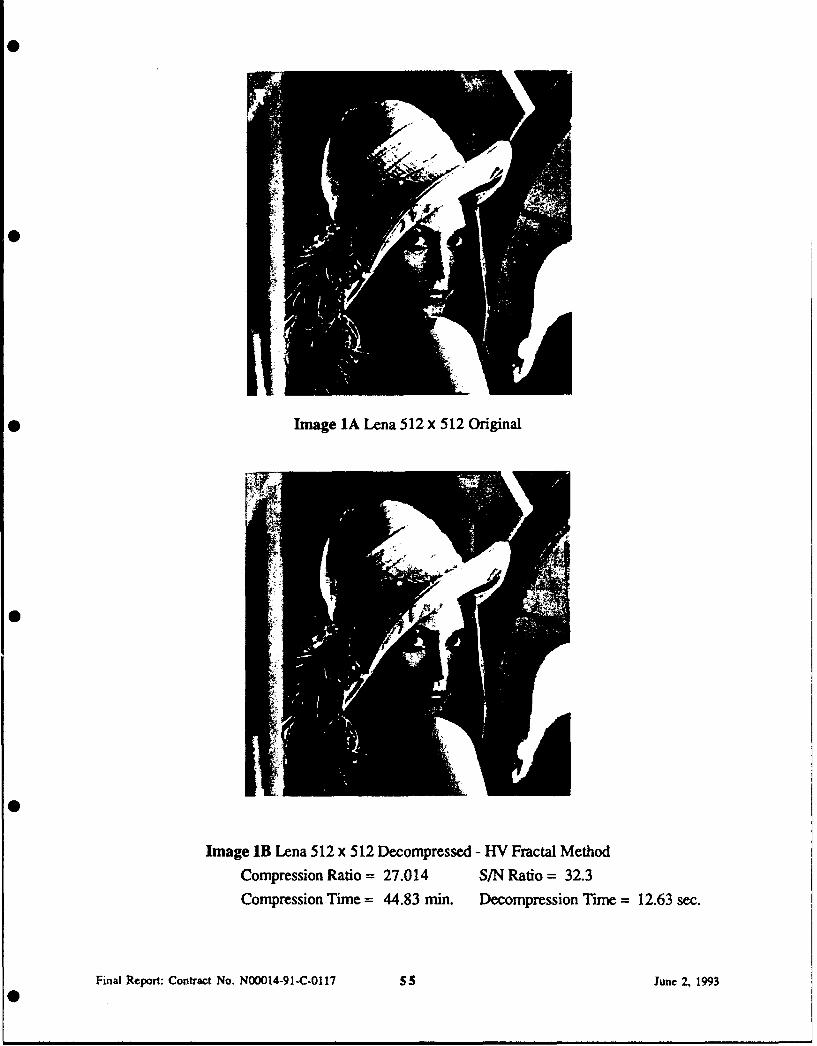
0i

Image 1A Lena 512 x 512 Original

S1

Image 1B Lena 512 x 512 Decompressed - HV Fractal Method

Compression Ratio = 27.014 S/N Ratio = 32.3Compression Time = 44.83 min. Decompression Time = 12.63 sec.


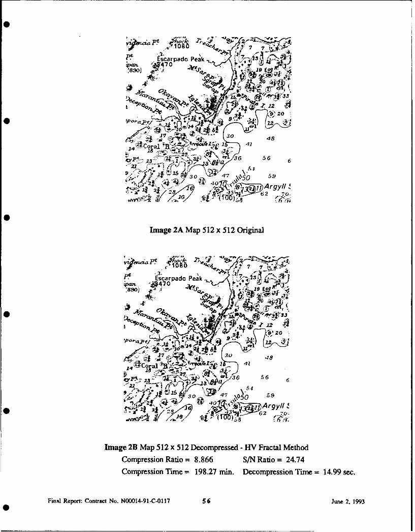
St

' f% 7A

P. tscarpado Peak-, 1 " s

-. 70 !z U. * '4•

24"" 08 ... '.

? rv•, .

&. Ecrpd Peak 48•

~ 'Cral a ~41

.14. •9 , ,..

9 ~ 49

~, /.,,.,~4 5

,: l'37; 1-

...- •- .• .• ., , •

23 ~*:f>JKr ~/36 56 64ý' 546

47' '50 59

* 4O~( W.,11 ~Argyll21d7 47 -8 ~ 62

Image 2B Map 512 x 512 Decompressed - ii Fractal Method

Compression Ratio = 8.866 S/N Ratio = 24.74

Compression Time = 198.27 min. De~compression Time = 14.99 sec.

Final Report: Contract No. N00014-91-C-0117 $56 June 2, 1993

Sz

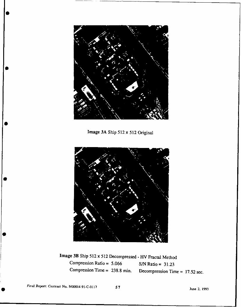
0

Image 3A Ship 512 x 512 Original

0!

0I

Image 3B Ship 512 x 512 Decompressed - HV Fractal MethodCompression Ratio = 5.066 S/N Ratio = 31.23Compression Time = 238.8 min. Decompression Time = 17.52 sec.

Final Report: Contract No. N00014-91-C-0117 57 June 2, 19930 ,,

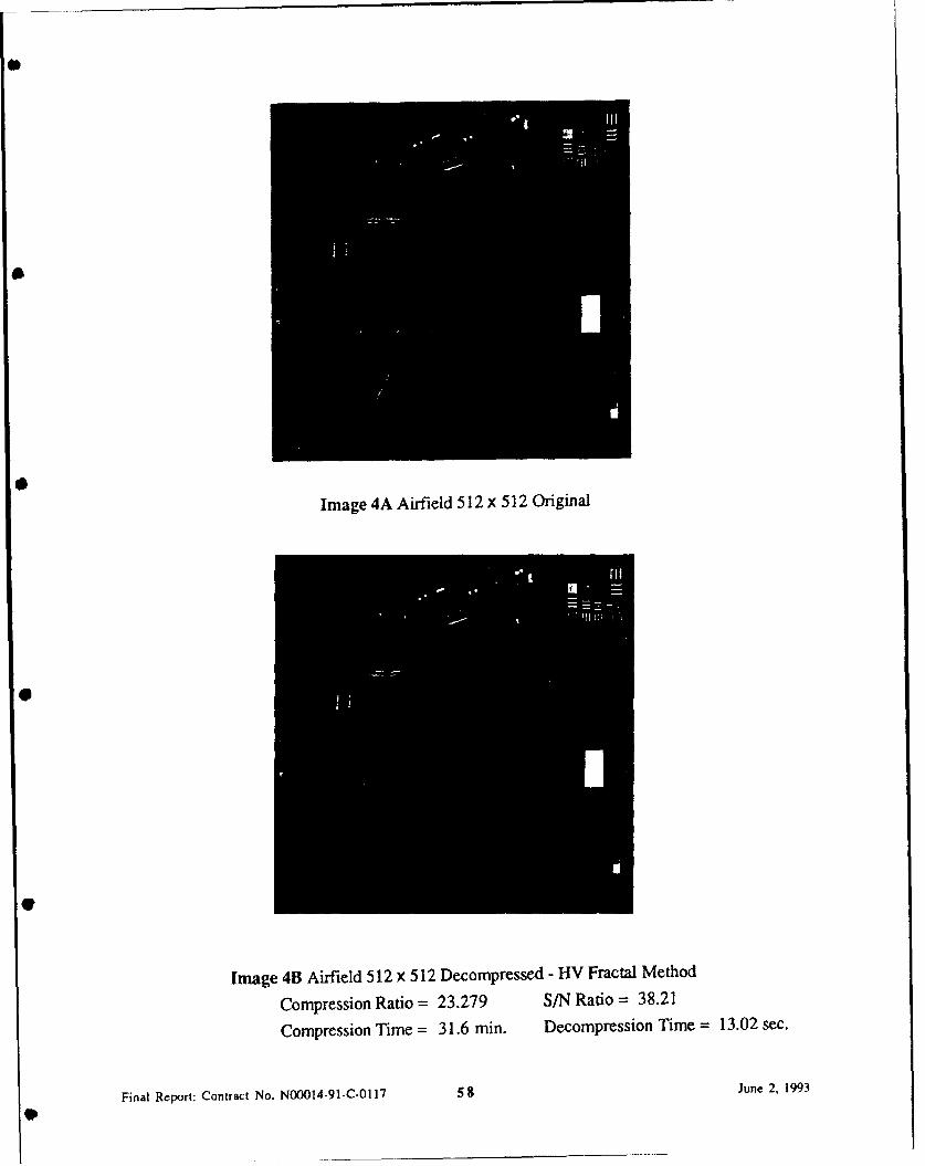
0

Image 4A Airfield 512 x 512 Original

Image 4B Airfield 512 x 512 Decompressed - HV Fractal Method


Compression Time = 31.6 min. Decompression Time = 13.02 sec.


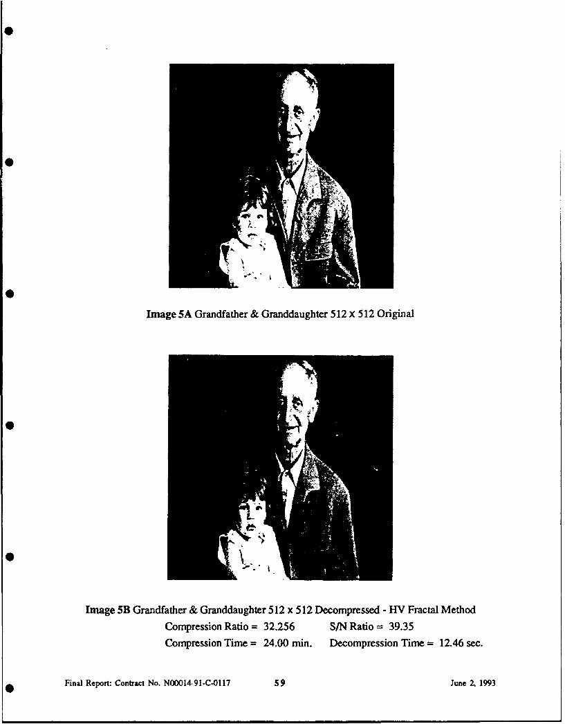
Image 5A Grandfather & Granddaughter 512 x 512 Original

Image 5B Grandfather & Granddaughter 512 x 512 Decompressed - HV Fractal Method


Compression Time = 24.00 min. Decompression Time = 12.46 sec.


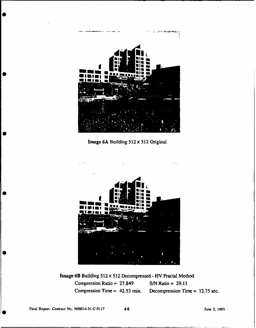
Image 6A Building 512 x 512 Original

Iinwin

Image 6B Building 512 x 512 Decompressed - RV Fractal, MethodCompression Ratio = 27.849 S/N Ratio = 29.11Compression Time = 42.53 min. Decompression Time = 12.75 sec.

Final Report: Contrac~t No. N00014-91-C-0117 60 June 2, 1993

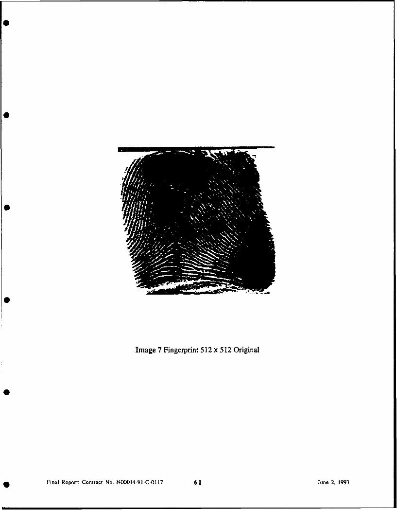
Image 7 Fingerprint 512 x 512 Original

*Final Report: Contract No. N00014-91-C-0117 61 June 2, 1993

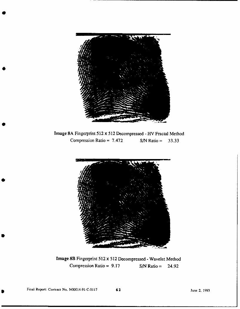
Image 8A Fingerprint 512 x 512 Decompressed - HV Fractal Method

Compression Ratio 7.472 S/N Ratio = 33.33

Image 8B Fingerprint 512 x 512 Decompressed - Wavelet Method



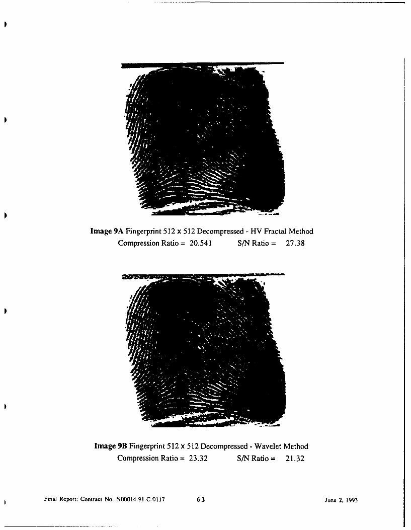
IA

IJ

Image 9A Fingerprint 512 x 512 Decompressed - HV Fractal Method


II

II

Image 9B Fingerprint 512 x 512 Decompressed - Wavelet Method



Documents

Image Compression Using Fractals and Wavelets · Image Compression Using Fractals and Wavelets ... A002 Final Report titled "Image Compression Using Fractals and Wavelets" ... 5.0