Induction Acceleration for Beam-Orbit Control

誘導加速による電子ビーム軌道の位置制御誘導加速による電子ビーム軌道の位置制御誘導加速による電子ビーム軌道の位置制御誘導加速による電子ビーム軌道の位置制御

広島大学理学研究科

物理科学専攻

M1179029

松野松野松野松野 聖史聖史聖史聖史

Department of Physics, Faculty of Science, Hiroshima University

Seiji Matsuno

2000-2001

2

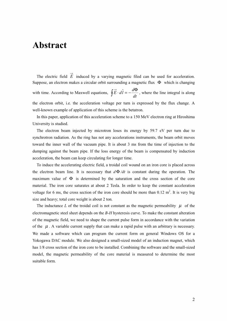
Abstract

The electric field E induced by a varying magnetic filed can be used for acceleration.

Suppose, an electron makes a circular orbit surrounding a magnetic flux Φ which is changing

with time. According to Maxwell equations, ∫Φ−=⋅

dt

dldE , where the line integral is along

the electron orbit, i.e. the acceleration voltage per turn is expressed by the flux change. A

well-known example of application of this scheme is the betatron.

In this paper, application of this acceleration scheme to a 150 MeV electron ring at Hiroshima

University is studied.

The electron beam injected by microtron loses its energy by 59.7 eV per turn due to

synchrotron radiation. As the ring has not any accelerations instruments, the beam orbit moves

toward the inner wall of the vacuum pipe. It is about 3 ms from the time of injection to the

dumping against the beam pipe. If the loss energy of the beam is compensated by induction

acceleration, the beam can keep circulating for longer time.

To induce the accelerating electric field, a troidal coil wound on an iron core is placed across

the electron beam line. It is necessary that d Φ /dt is constant during the operation. The

maximum value of Φ is determined by the saturation and the cross section of the core

material. The iron core saturates at about 2 Tesla. In order to keep the constant acceleration

voltage for 6 ms, the cross section of the iron core should be more than 0.12 m2. It is very big

size and heavy; total core weight is about 2 ton.

The inductance L of the troidal coil is not constant as the magnetic permeability µ of the

electromagnetic steel sheet depends on the B-H hysteresis curve. To make the constant alteration

of the magnetic field, we need to shape the current pulse form in accordance with the variation

of the µ . A variable current supply that can make a rapid pulse with an arbitrary is necessary.

We made a software which can program the current form on general Windows OS for a

Yokogawa DAC module. We also designed a small-sized model of an induction magnet, which

has 1/8 cross section of the iron core to be installed. Combining the software and the small-sized

model, the magnetic permeability of the core material is measured to determine the most

suitable form.

3

Contents

Abstract 2

Chapter 1 Introduction 4

Chapter 2 Possible application of induction acceleration to REFER 5

2.1 The 150 MeV electron ring REFER 5 2.2 The present situation of REFER 6 2.3 The improvement plan 8

Chapter 3 The application of induction acceleration

scheme to REFER 9 3.1 The principle of induction acceleration 9 3.2 Saturation of the core material 9 3.3 The B-H curve 11 3.4 Determination of magnetic permeability 12 3.5 The energy conservation 14 3.6 A current form generator 17

Chapter 4 Experiments, Results, and Discussions 18

4.1 The magnet cores 18 4.2 Setup of the experiments 19 4.3 Results and Discussions 20

Chapter 5 Conclusion 27

Acknowledgements 28

References 29

Appendix 30 A Software for Yokogawa DAC module 30

4

Chapter 1 Introduction

New types of induction accelerators are recently attracting interest: A novel induction

acceleration in a fixed-field alternating-gradient magnet was proposed by T. Ohkawa et

al. It was the first application of this scheme to a circular accelerator [1][2]. Another

example is a 3.6 MeV induction LINAC constructed in collaboration of High Energy

Accelerator Research Institute (KEK) and Japan Atomic Energy Research Institute

(JAERI). Now, the induction synchrotron for KEK 12 GeV Proton Synchrotron is being

constructed [3][4][5]. To accelerate protons up to 12 GeV is a hard task and we need to

develop many big induction magnets and switching systems for high frequency current.

On the other hand, with this scheme we can easily give a small amount of energy

enough to compensate the synchrotron radiation loss at a small-scale circular storage

ring. We can also control the position of the beam orbit by adjusting the accelerating

voltage.

We examine the applicability of such an acceleration scheme to a 150 MeV

small-scale electron ring at Hiroshima University which is called REFER, Relativistic

Electron Facility for Education and Research.

In Chapter 2, we discuss about the actual situation of the REFER ring and the

significance of application of induction acceleration. In Chapter 3, we discuss about the

possible difficulties to be overcome. In Chapter 4, we discuss about the measurement

using the small-sized model of an induction magnet.

5

Chapter 2 Possible application of induction acceleration to

REFER

2.1 The 150MeV electron ring REFER

REFER is an electron beam ring at Hiroshima University in which an electron beam

goes along the circular orbit of circumference of 13.5 m. This ring has neither an

acceleration structure nor an electron gun. It accepts a 150 MeV electron beam from a

microtron that belongs to Hiroshima Synchrotron Radiation Center, Hiroshima

University (HiSOR).

The injection beam parameters depend on those of microtron as shown Table1-1 [6],

while Table1-2 shows the REFER basic parameters [7].

Output Beam Energy 150 MeV Input Beam Energy 80 keV Peak Beam Current 2-10 mA Beam Pulse Width 0.2-2 μsec Repetition 0.2-100Hz Beam Emmitance 0.5πmm-mr ( 1σ) Energy Dispersion ±0.1％ ( 1σ) Mag. Field of Bending Mag. 1.23 T Magnetic Field Gradient 0.14 T/m Pole Gap of Bending Mag. 10 mm Number of Turns 25 Energy Gain per Turn 6 MeV Accelerator Structure 8 Cell Side-Coupled Cavity Accelerator Bore 10 mm RF Frequency 2856 MHz RF Field Gradient 15 MV/m RF Wall Loss 1.5 MW ( Max. ) Beam Loading 2.0 MW ( Max. )

Table1-1 The microtron parameters

6

Electron Energy 150 MeV Length of Beam Orbit 13.5 m Long Straight Section 2.5 m Short Straight Section 0.7 m Field of Bending Mag. 0.67 T Radius of Curvature 0.75 m Frequency 10-100 Hz Horizontal Tune 1.39 Vertical Tune 1.65 Number of Bending Mag. 8 Value n of Bending Mag. 0.55

Table1-2 The REFER basic parameters

This ring is used to study parametric x-rays, laser compton scattering, and the

development of a x-ray source based on new mechanism. The ring has an inner target

set in a vacuum chamber placed on the beam orbit.

2.2 The present situation of REFER

The electron beam injected by the microtron loses its energy by 59.7 eV per turn due

to synchrotron radiation. As the ring has not any acceleration instruments, the beam

orbit moves toward the inner wall of the vacuum pipe.

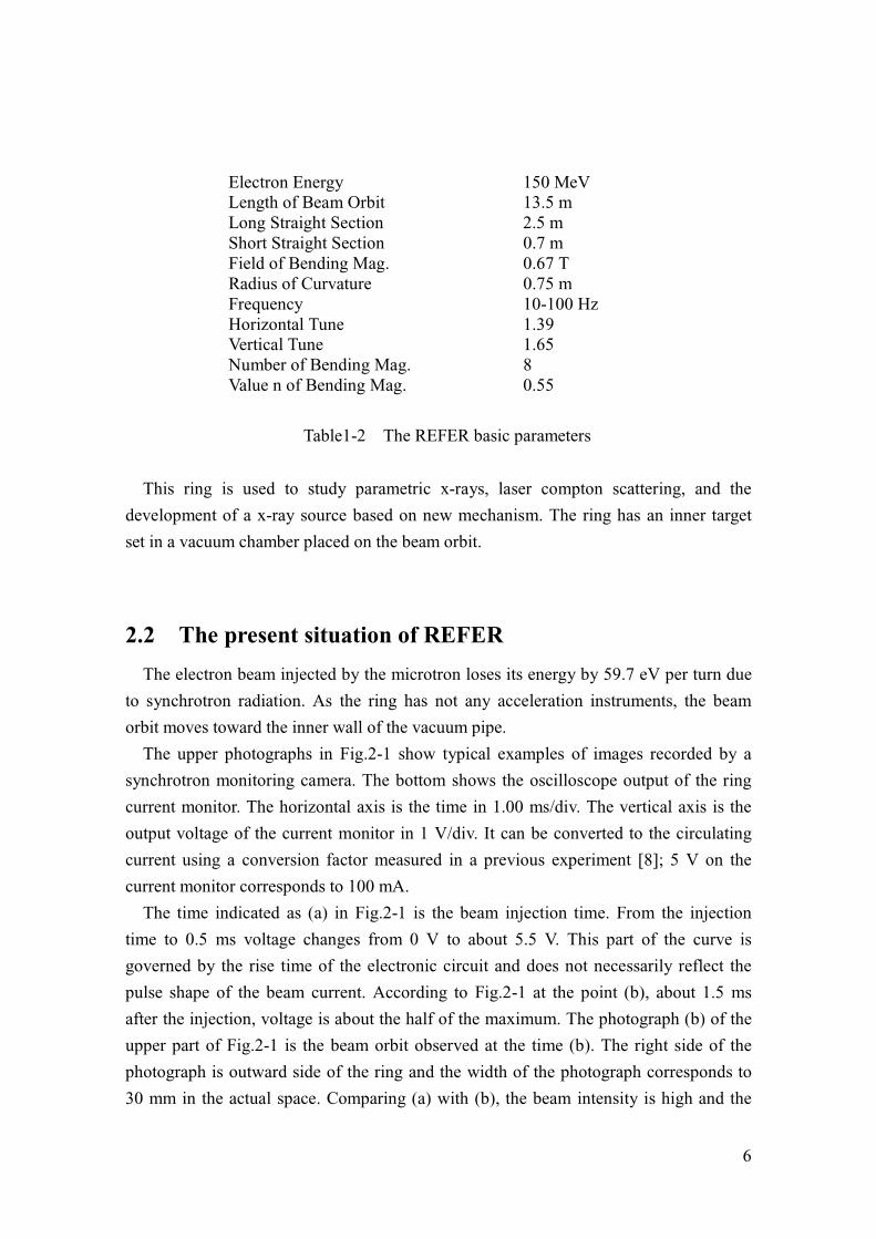
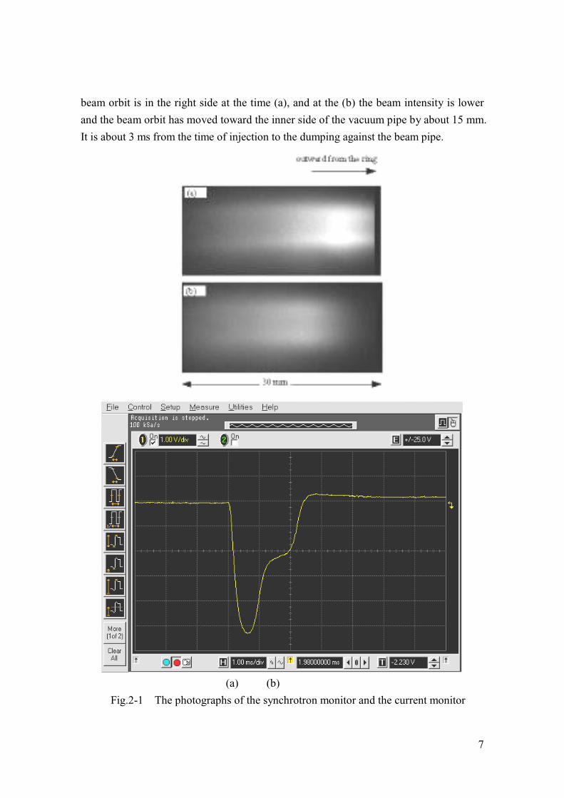
The upper photographs in Fig.2-1 show typical examples of images recorded by a

synchrotron monitoring camera. The bottom shows the oscilloscope output of the ring

current monitor. The horizontal axis is the time in 1.00 ms/div. The vertical axis is the

output voltage of the current monitor in 1 V/div. It can be converted to the circulating

current using a conversion factor measured in a previous experiment [8]; 5 V on the

current monitor corresponds to 100 mA.

The time indicated as (a) in Fig.2-1 is the beam injection time. From the injection

time to 0.5 ms voltage changes from 0 V to about 5.5 V. This part of the curve is

governed by the rise time of the electronic circuit and does not necessarily reflect the

pulse shape of the beam current. According to Fig.2-1 at the point (b), about 1.5 ms

after the injection, voltage is about the half of the maximum. The photograph (b) of the

upper part of Fig.2-1 is the beam orbit observed at the time (b). The right side of the

photograph is outward side of the ring and the width of the photograph corresponds to

30 mm in the actual space. Comparing (a) with (b), the beam intensity is high and the

7

beam orbit is in the right side at the time (a), and at the (b) the beam intensity is lower

and the beam orbit has moved toward the inner side of the vacuum pipe by about 15 mm.

It is about 3 ms from the time of injection to the dumping against the beam pipe.

(a) (b)

Fig.2-1 The photographs of the synchrotron monitor and the current monitor

8

2.3 The improvement plan

We want to improve the REFER ring, at least in the following 2 points.

(1) To increase the beam life time

(2) To make the orbit radius constant without depending on time

In our plan the loss energy 59.7 eV per turn due to synchrotron radiation of the beam

is compensated using the scheme of the induction acceleration. If the loss energy of the

beam is properly compensated by induction acceleration, the beam can keep circulating

for longer time. Furthermore, we will be able to control the beam orbit by adjusting the

rate of the flux change in the induction coil.

Another point is that we may possibly reduce the unwanted radiation caused by the

collision of the low energy electrons with the vacuum pipe by properly controlling the

beam dumping time.

9

Chapter 3 The application of induction acceleration

scheme to REFER

3.1 The principle of induction acceleration

The principle of induction acceleration is derived from the Maxwell equations. The

electric field E induced by a varying magnetic filed flux is related to the electromotive force V0 in the following way;

0)( Vdt

dldE =Φ−=⋅∫ . (3-1)

This means that an electron is accelerated by eV0, if it makes a circular orbit, following

the integration path in (3-1), surrounding a magnetic flux Φ that is changing with time.

For applying to REFER we require the voltage V0 to be 59.7 V.

3.2 Saturation of the core material

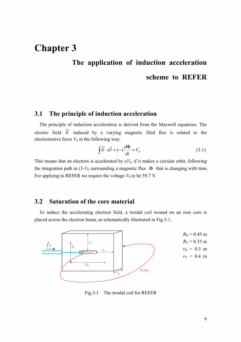
To induce the accelerating electron field, a troidal coil wound on an iron core is

placed across the electron beam, as schematically illustrated in Fig.3-1.

RH = 0.45 m

RV = 0.35 m

rH = 0.3 m

rV = 0.4 m

Fig.3-1 The troidal coil for REFER

I R V

R H

rH

rH

rV

10

The iron core size is determined the maximum value of the magnetic flux density B.

As described in Chapter 2 it is necessary that dt

dΦ is constant during at least 3 ms. The

maximum value of Φ is determined by the saturation and the cross section S of the

core material.

According to Φ = BS , S = rHrV = 0.12 m2 ,

497

7.590

≈

==Φ=

dt

dBdt

SdB

dt

dV

. (3-2)

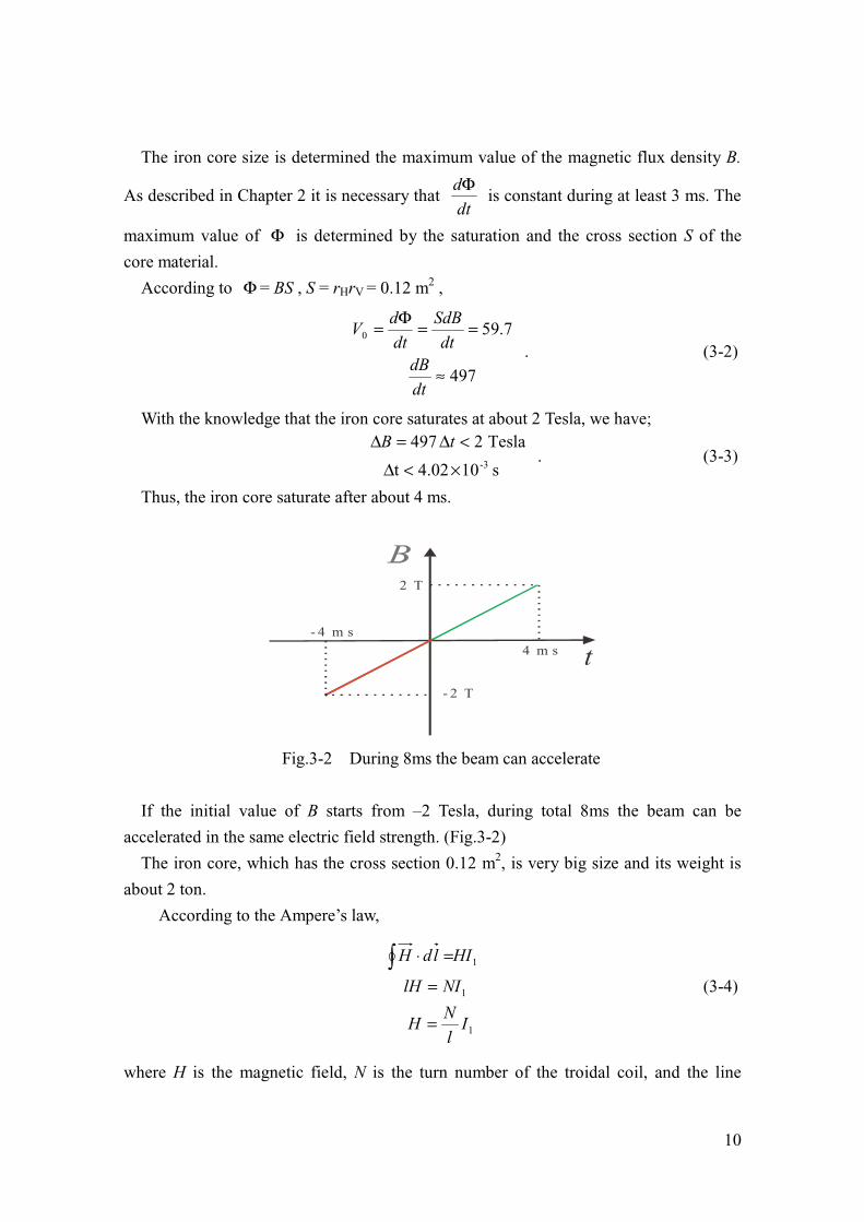
With the knowledge that the iron core saturates at about 2 Tesla, we have;

s104.02t

Tesla24973-×<∆

<∆=∆ tB . (3-3)

Thus, the iron core saturate after about 4 ms.

t- 4 m s

2 T

- 2 T

4 m s

Fig.3-2 During 8ms the beam can accelerate

If the initial value of B starts from –2 Tesla, during total 8ms the beam can be

accelerated in the same electric field strength. (Fig.3-2)

The iron core, which has the cross section 0.12 m2, is very big size and its weight is

about 2 ton.

According to the Ampere’s law,

1

1

1

Il

NH

NIlH

HIldH

=

=

=⋅∫ (3-4)

where H is the magnetic field, N is the turn number of the troidal coil, and the line

11

integral is along the magnetic flux i.e. l is the average length of the core.

The magnetic flux Φ that goes through the coil is expressed by

1Il

NSHSBS µµ ===Φ (3-5)

where µ is the magnetic permeability of the core material.

The inductance L of the coil is

.2Nl

SL µ= (3-6)

If L does not depend on time, a constant electron field 59.7 V to accelerate the

electron beam per turn might be achieved by satisfying the relations

A/s7.59

7.591

)(

1

10

L

N

dt

dIdt

dI

NL

dt

dV

×=∴

==Φ−= . (3-7)

Obviously, the above considerations are not enough to determine the rate of change of

the magnet current I1 because the inductance is time dependent due to the nonlinear B-H

relation as discussed in the next section.

3.3 The B-H curve

In this section, we study the dependence of the B-H hysteresis of the core material.

The inductance L of the troidal coil is not constant as the magnetic permeability µ

of the electromagnetic steel sheet depends on H. In the induction acceleration we must

supply a rapidly varying current pulse to the troidal magnet. Ordinary iron cores suffer

from the effect of the eddy current. We need the iron core that has a less effect of the

eddy current and we chose the electromagnetic steel sheet of silicon steel is

KAWATETSU 30RG120. We make a core by stacking the 0.3 mm thick sheets with

varnished insulator on the surface.

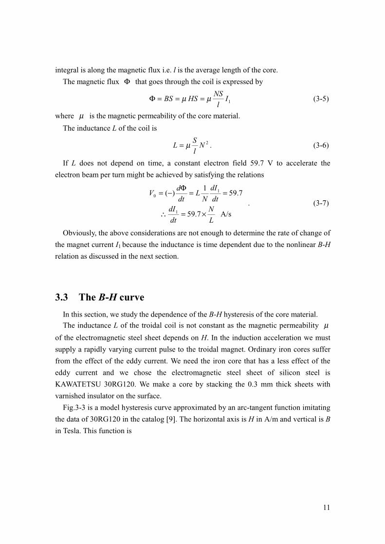
Fig.3-3 is a model hysteresis curve approximated by an arc-tangent function imitating

the data of 30RG120 in the catalog [9]. The horizontal axis is H in A/m and vertical is B

in Tesla. This function is

12

===

−= −

232.2

2.6

114.1

.tan 1

c

b

a

c

bHaB

(3-8)

In this consideration the current goes up only and the value of the core saturation is

1.75 Tesla. When the current goes down the B-H curve is different from (3-8).

-40 -30 -20 -10 0 10 20 30 40-2

-1

0

1

2

B [Tesla]

H [A/m]

Fig.3-3 A model hysteresis curve of 30RG120 when the current goes up only

3.4 Determination of magnetic permeability

The coil turn number to be installed beam line is 2. (N = 2) From Ampere law the

relationship between H and I1 is

.25.1 11 IIl

NH == (3-9)

As the magnetic permeability µ is the inclination of the B-H curve,

.

12

−+

=∂∂=

c

bH

a

H

Bµ (3-10)

According to Fig.3-3, we see that µ is almost constant at the neighborhood of the

point of B = 0. Thus, 114.10

0==

∂∂=

==

aH

B

BB

µ , we regard as the inclination is

13

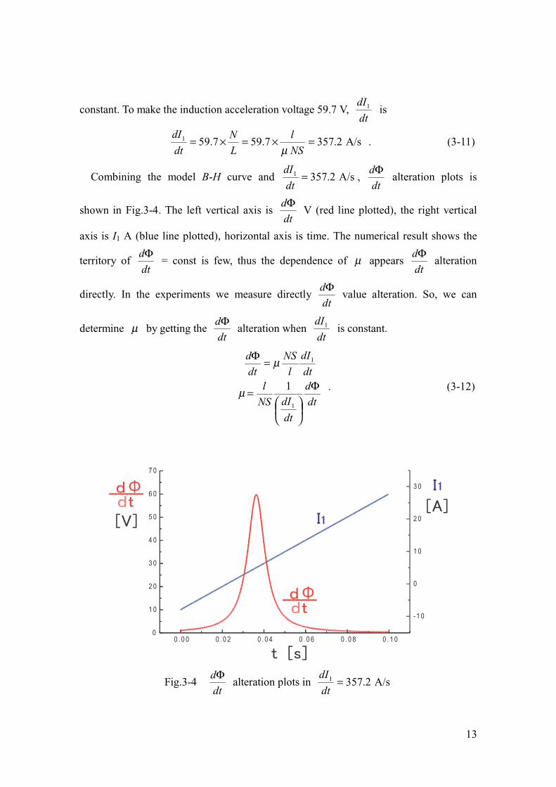
constant. To make the induction acceleration voltage 59.7 V, dt

dI1 is

A/s2.3577.597.591 =×=×=NS

l

L

N

dt

dI

µ . (3-11)

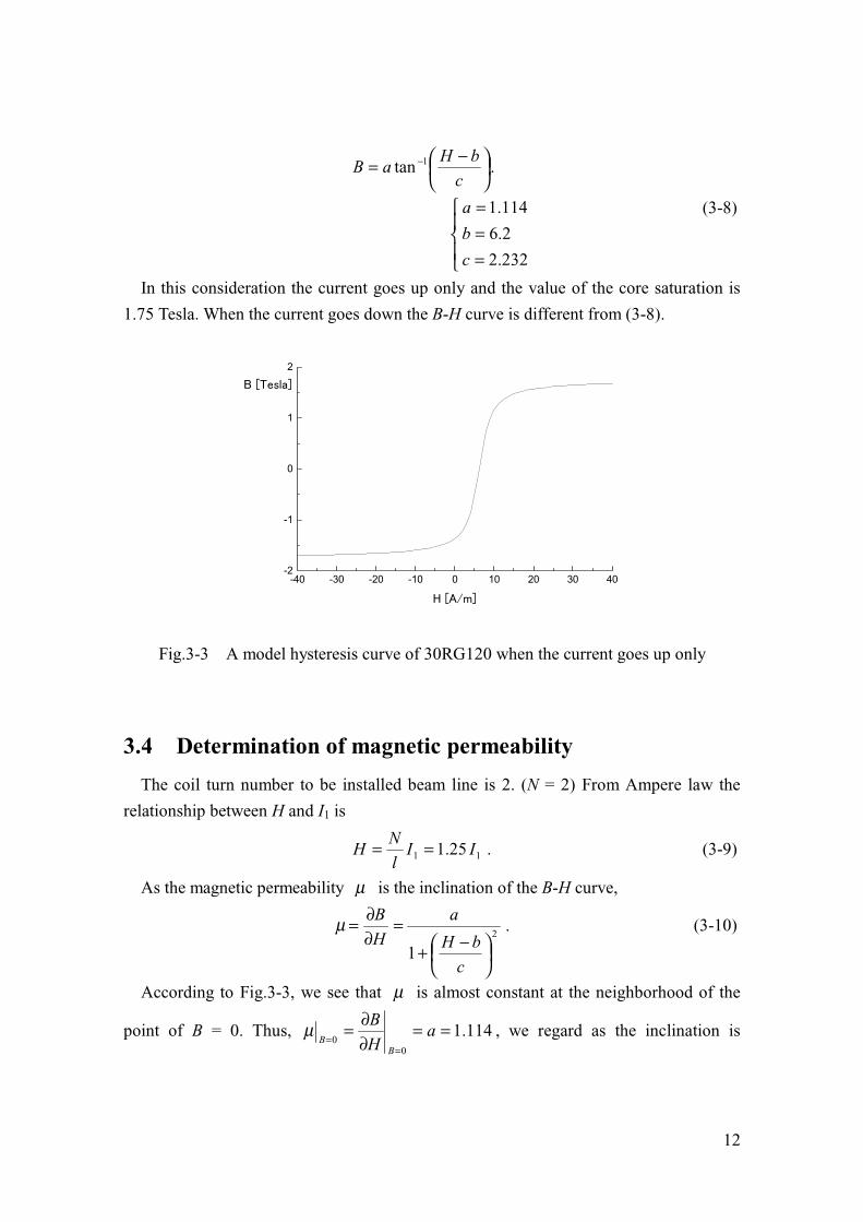
Combining the model B-H curve and A/s2.3571 =dt

dI,

dt

dΦ alteration plots is

shown in Fig.3-4. The left vertical axis is dt

dΦ V (red line plotted), the right vertical

axis is I1 A (blue line plotted), horizontal axis is time. The numerical result shows the

territory of dt

dΦ = const is few, thus the dependence of µ appears

dt

dΦ alteration

directly. In the experiments we measure directly dt

dΦ value alteration. So, we can

determine µ by getting the dt

dΦ alteration when

dt

dI1 is constant.

dt

d

dt

dINS

ldt

dI

l

NS

dt

d

Φ

=

=Φ

1

1

1µ

µ

. (3-12)

0 . 0 0 0 . 0 2 0 . 0 4 0 . 0 6 0 . 0 8 0 . 1 00

1 0

2 0

3 0

4 0

5 0

6 0

7 0

-1 0

0

1 0

2 0

3 0ｄΦ

[V][A]

I

ｄΦ

I

Fig.3-4 dt

dΦ alteration plots in A/s2.3571 =

dt

dI

14

3.5 The energy conservation

In section 3.4, dt

dI1 and V1 are determined independently from the beam current I2 to

accelerate. The beam-energy loss by the synchrotron radiation is directly proportional to

the value of the beam current, on the other hand the providing power V1I1 is not

concerned with I2 at all. We wonder about the energy relationship between revenue and

expenditure. In this section we discuss about the energy conservation. We use a

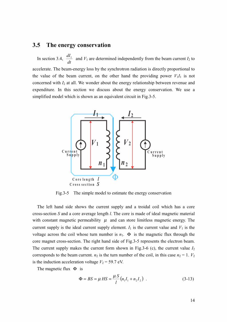
simplified model which is shown as an equivalent circuit in Fig.3-5.

V 1 V 2

n 2n 1

C u r r e n tS u p p ly

I2I1

C o r e l e n g t h lC r o s s s e c t i o n S

C u r r e n tS u p p ly

Fig.3-5 The simple model to estimate the energy conservation

The left hand side shows the current supply and a troidal coil which has a core

cross-section S and a core average length l. The core is made of ideal magnetic material

with constant magnetic permeability µ and can store limitless magnetic energy. The

current supply is the ideal current supply element. I1 is the current value and V1 is the

voltage across the coil whose turn number is n1. Φ is the magnetic flux through the

core magnet cross-section. The right hand side of Fig.3-5 represents the electron beam.

The current supply makes the current form shown in Fig.3-6 (c), the current value I2

corresponds to the beam current. n2 is the turn number of the coil, in this case n2 = 1. V2

is the induction acceleration voltage V2 = 59.7 eV.

The magnetic flux Φ is

( )2211 InInl

SHSBS +===Φ µµ . (3-13)

15

The voltage produced by the time variation of Φ is

+=Φ=

dt

dIn

dt

dIn

l

Sn

dt

dnV 2

21

11

11

µ . (3-14)

+=Φ=

dt

dIn

dt

dIn

l

Sn

dt

dnV 2

21

12

22

µ . (3-15)

From V1 and V2,

11

22 V

n

nV = . (3-16)

Suppose we give the one period triangle current form I1,

≤≤+−

≤≤−

=

a

bt

a

bbat

a

btbat

I42

3

20

1 . (3-17)

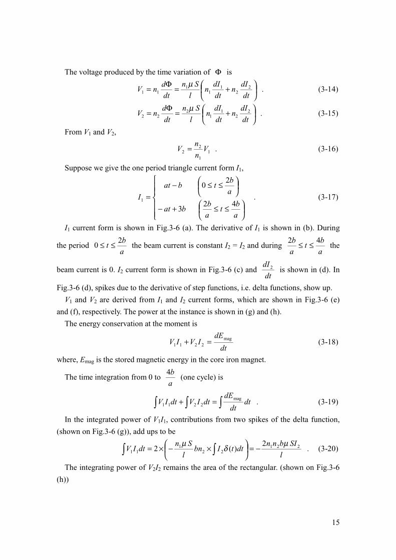
I1 current form is shown in Fig.3-6 (a). The derivative of I1 is shown in (b). During

the period a

bt

20 ≤≤ the beam current is constant I2 = I2 and during

a

bt

a

b 42 ≤≤ the

beam current is 0. I2 current form is shown in Fig.3-6 (c) and dt

dI 2 is shown in (d). In

Fig.3-6 (d), spikes due to the derivative of step functions, i.e. delta functions, show up.

V1 and V2 are derived from I1 and I2 current forms, which are shown in Fig.3-6 (e)

and (f), respectively. The power at the instance is shown in (g) and (h).

The energy conservation at the moment is

dt

dEIVIV mag

2211 =+ (3-18)

where, Emag is the stored magnetic energy in the core iron magnet.

The time integration from 0 to a

b4 (one cycle) is

∫∫∫ =+ dtdt

dEdtIVdtIV mag

2211 . (3-19)

In the integrated power of V1I1, contributions from two spikes of the delta function,

(shown on Fig.3-6 (g)), add ups to be

l

SIbnndttIbn

l

SndtIV 221

221

11

2)(2

µδµ −=

×−×= ∫∫ . (3-20)

The integrating power of V2I2 remains the area of the rectangular. (shown on Fig.3-6

(h))

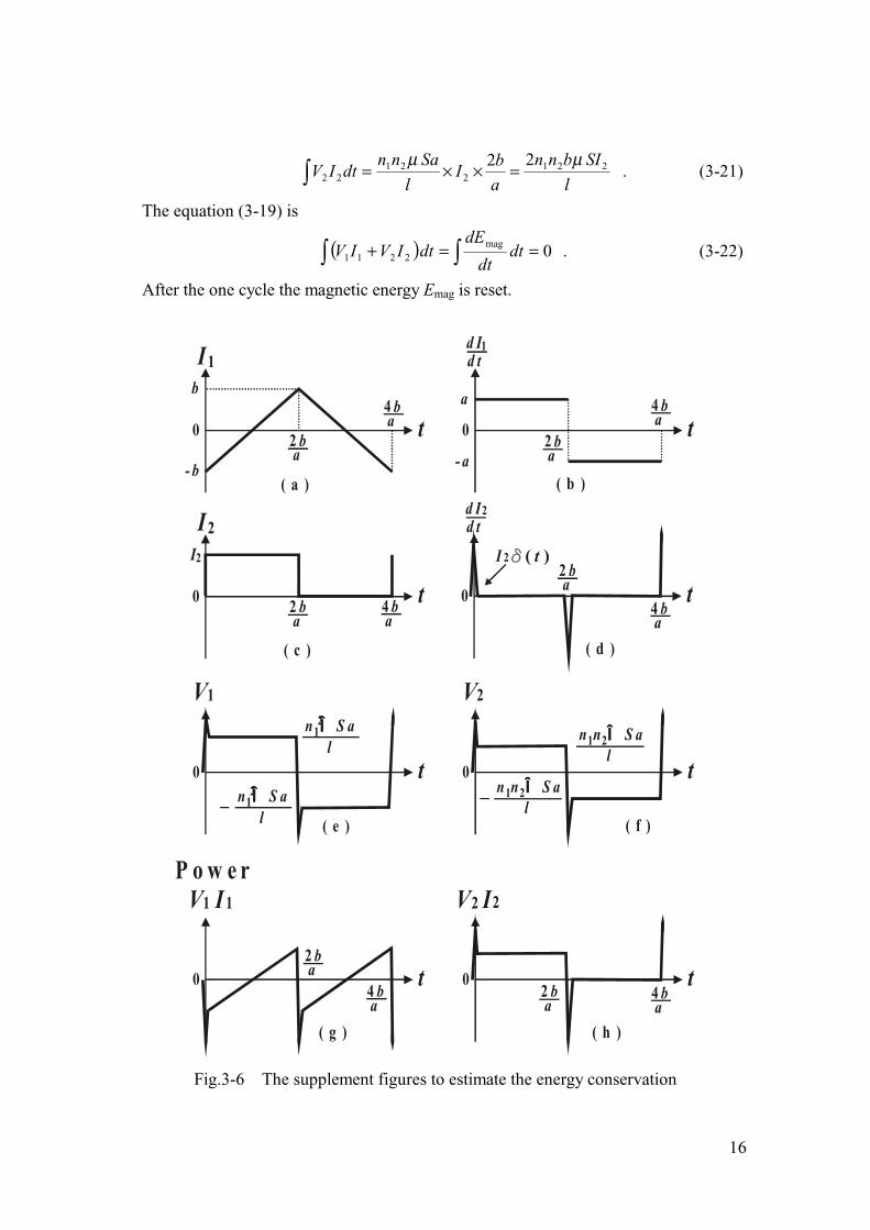
16

l

SIbnn

a

bI

l

SanndtIV 221

221

22

22 µµ=××=∫ . (3-21)

The equation (3-19) is

( ) 0mag2211 ==+ ∫∫ dt

dt

dEdtIVIV . (3-22)

After the one cycle the magnetic energy Emag is reset.

I1

t04 ba

b

- b

2 ba

I2

t04 ba

2 ba

I2

t0

d Id t

a

- a

1

t0

d Id t

2

t0

V1

n S aμμμμl

21

n S aμμμμl

21

( a ) ( b )

( c ) ( d )

( e )

t0

V2

n n S aμμμμl

21

n n S aμμμμl

21

( f )

P o w e r

t0

V1

( g )

t0

2

( h )

I 1 V I2

2 ba

4 ba

2 ba

4 ba

4 ba

2 ba

2 ba

4 ba

I 2

Fig.3-6 The supplement figures to estimate the energy conservation

17

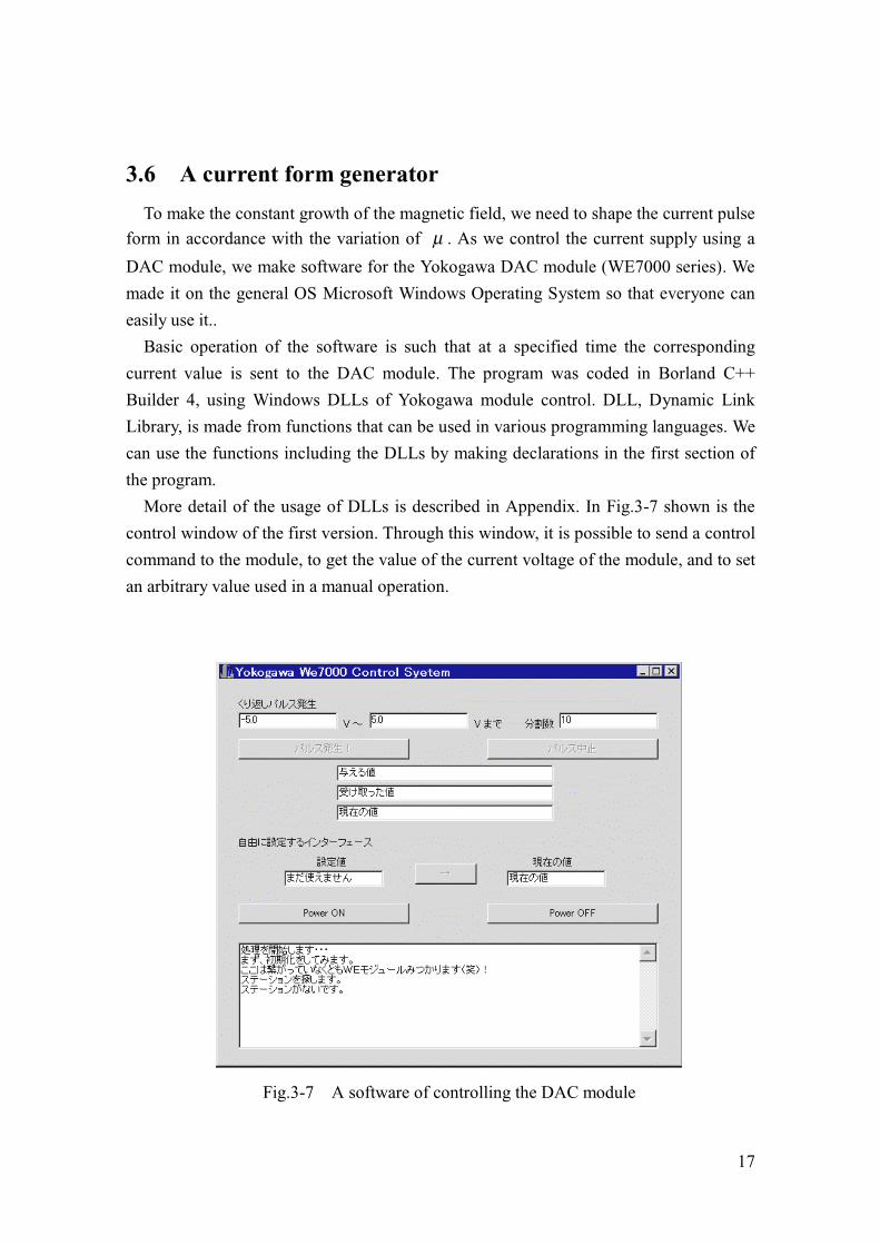
3.6 A current form generator

To make the constant growth of the magnetic field, we need to shape the current pulse

form in accordance with the variation of µ . As we control the current supply using a

DAC module, we make software for the Yokogawa DAC module (WE7000 series). We

made it on the general OS Microsoft Windows Operating System so that everyone can

easily use it..

Basic operation of the software is such that at a specified time the corresponding

current value is sent to the DAC module. The program was coded in Borland C++

Builder 4, using Windows DLLs of Yokogawa module control. DLL, Dynamic Link

Library, is made from functions that can be used in various programming languages. We

can use the functions including the DLLs by making declarations in the first section of

the program.

More detail of the usage of DLLs is described in Appendix. In Fig.3-7 shown is the

control window of the first version. Through this window, it is possible to send a control

command to the module, to get the value of the current voltage of the module, and to set

an arbitrary value used in a manual operation.

Fig.3-7 A software of controlling the DAC module

18

Chapter 4 Experiments, Results, and Discussions

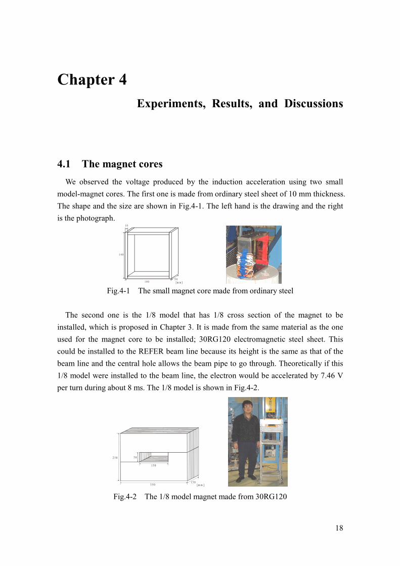
4.1 The magnet cores

We observed the voltage produced by the induction acceleration using two small

model-magnet cores. The first one is made from ordinary steel sheet of 10 mm thickness.

The shape and the size are shown in Fig.4-1. The left hand is the drawing and the right

is the photograph.

1 4 05 0

1 4 0

1 0

[ m m ] Fig.4-1 The small magnet core made from ordinary steel

The second one is the 1/8 model that has 1/8 cross section of the magnet to be

installed, which is proposed in Chapter 3. It is made from the same material as the one

used for the magnet core to be installed; 30RG120 electromagnetic steel sheet. This

could be installed to the REFER beam line because its height is the same as that of the

beam line and the central hole allows the beam pipe to go through. Theoretically if this

1/8 model were installed to the beam line, the electron would be accelerated by 7.46 V

per turn during about 8 ms. The 1/8 model is shown in Fig.4-2.

2 5 0

3 5 0

5 0

1 5 0

1 5 0[ m m ]

Fig.4-2 The 1/8 model magnet made from 30RG120

19

The right hand is the photograph of the 1/8 model. The author of this work, who is

170 cm tall, is standing near by.

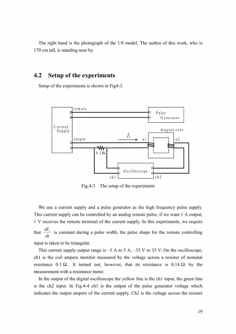
4.2 Setup of the experiments

Setup of the experiments is shown in Fig4-3.

C u r r e n tS u p p l y

0 . 1Ω

c h 1 c h 2

n 1 n 2

O s c i l l o s c o p e

m a g n e t c o r e

P u l s eG e n e r a t o r

r e m o t e

o u t p u tI1

Fig.4-3 The setup of the experiments

We use a current supply and a pulse generator as the high frequency pulse supply.

This current supply can be controlled by an analog remote pulse, if we want 1 A output,

1 V receives the remote terminal of the current supply. In this experiments, we require

that dt

dI1 is constant during a pulse width, the pulse shape for the remote controlling

input is taken to be triangular.

This current supply output range is –5 A to 5 A, –35 V to 35 V. On the oscilloscope,

ch1 is the coil ampere monitor measured by the voltage across a resister of nominal

resistance 0.1 Ω . It turned out, however, that its resistance is 0.14 Ω by the

measurement with a resistance meter.

In the output of the digital oscilloscope the yellow line is the ch1 input, the green line

is the ch2 input. In Fig.4-4 ch1 is the output of the pulse generator voltage which

indicates the output ampere of the current supply. Ch2 is the voltage across the resister

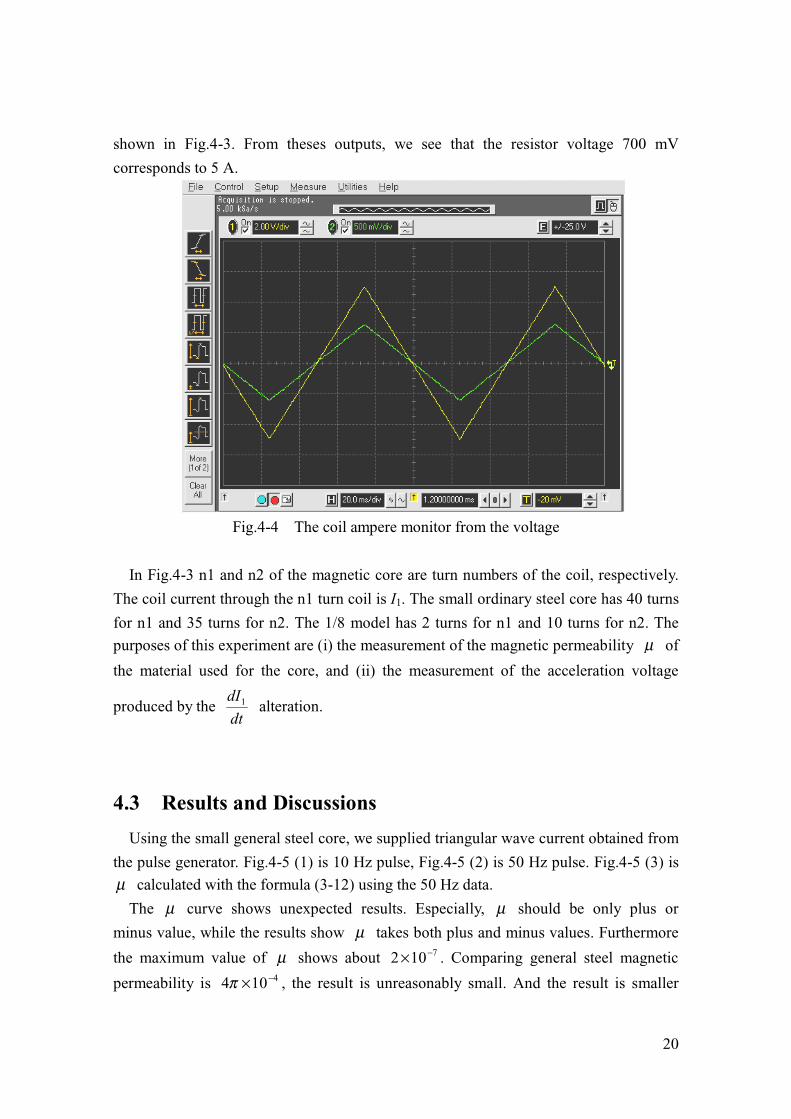
20

shown in Fig.4-3. From theses outputs, we see that the resistor voltage 700 mV

corresponds to 5 A.

Fig.4-4 The coil ampere monitor from the voltage

In Fig.4-3 n1 and n2 of the magnetic core are turn numbers of the coil, respectively.

The coil current through the n1 turn coil is I1. The small ordinary steel core has 40 turns

for n1 and 35 turns for n2. The 1/8 model has 2 turns for n1 and 10 turns for n2. The

purposes of this experiment are (i) the measurement of the magnetic permeability µ of

the material used for the core, and (ii) the measurement of the acceleration voltage

produced by the dt

dI1 alteration.

4.3 Results and Discussions

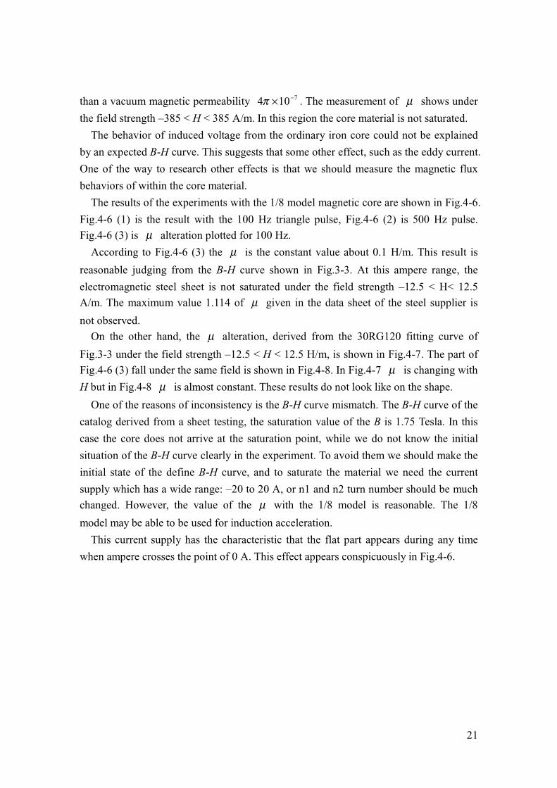
Using the small general steel core, we supplied triangular wave current obtained from

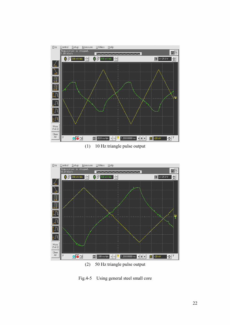
the pulse generator. Fig.4-5 (1) is 10 Hz pulse, Fig.4-5 (2) is 50 Hz pulse. Fig.4-5 (3) is

µ calculated with the formula (3-12) using the 50 Hz data.

The µ curve shows unexpected results. Especially, µ should be only plus or

minus value, while the results show µ takes both plus and minus values. Furthermore

the maximum value of µ shows about 7102 −× . Comparing general steel magnetic

permeability is 4104 −×π , the result is unreasonably small. And the result is smaller

21

than a vacuum magnetic permeability 7104 −×π . The measurement of µ shows under

the field strength –385 < H < 385 A/m. In this region the core material is not saturated.

The behavior of induced voltage from the ordinary iron core could not be explained

by an expected B-H curve. This suggests that some other effect, such as the eddy current.

One of the way to research other effects is that we should measure the magnetic flux

behaviors of within the core material.

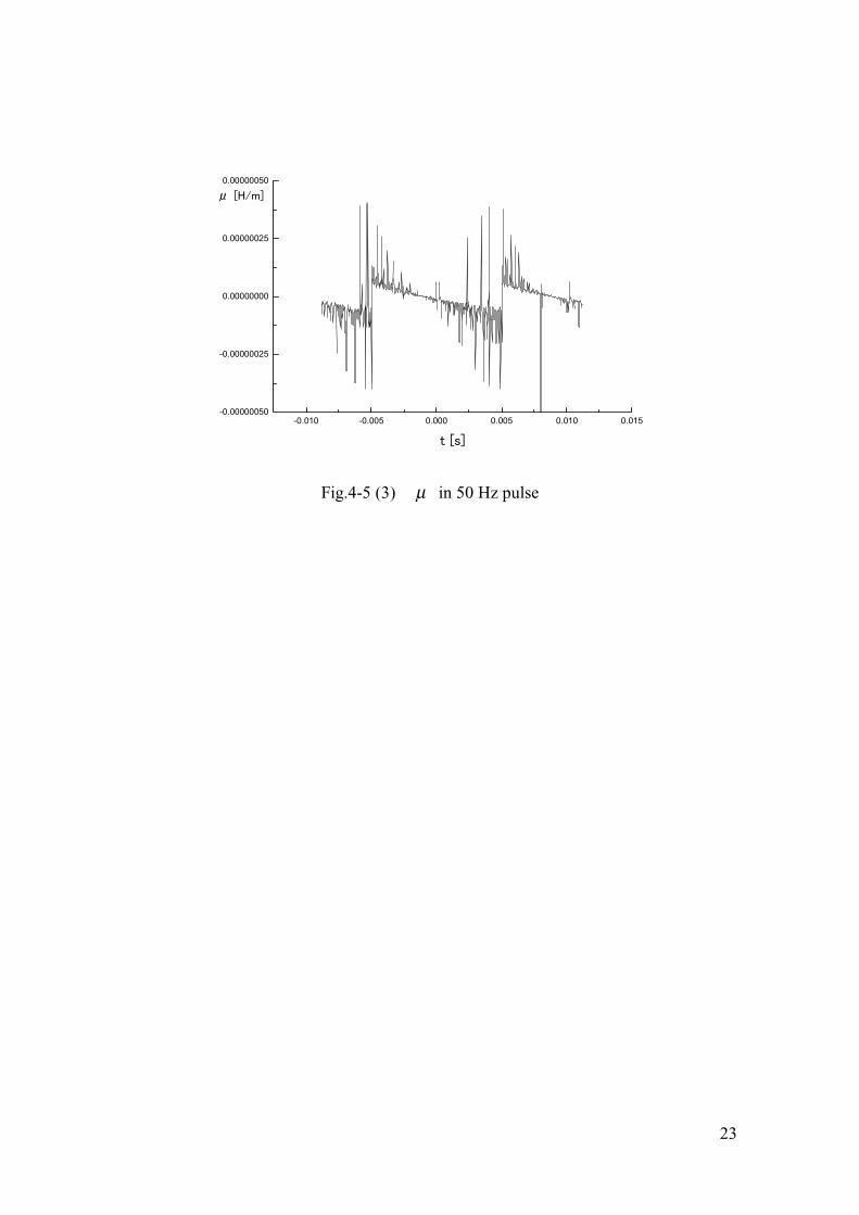
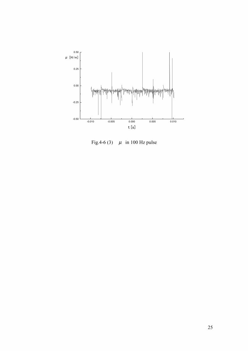
The results of the experiments with the 1/8 model magnetic core are shown in Fig.4-6.

Fig.4-6 (1) is the result with the 100 Hz triangle pulse, Fig.4-6 (2) is 500 Hz pulse.

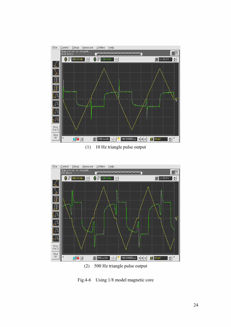
Fig.4-6 (3) is µ alteration plotted for 100 Hz.

According to Fig.4-6 (3) the µ is the constant value about 0.1 H/m. This result is

reasonable judging from the B-H curve shown in Fig.3-3. At this ampere range, the

electromagnetic steel sheet is not saturated under the field strength –12.5 < H< 12.5

A/m. The maximum value 1.114 of µ given in the data sheet of the steel supplier is

not observed.

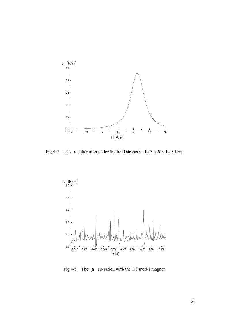
On the other hand, the µ alteration, derived from the 30RG120 fitting curve of

Fig.3-3 under the field strength –12.5 < H < 12.5 H/m, is shown in Fig.4-7. The part of

Fig.4-6 (3) fall under the same field is shown in Fig.4-8. In Fig.4-7 µ is changing with

H but in Fig.4-8 µ is almost constant. These results do not look like on the shape.

One of the reasons of inconsistency is the B-H curve mismatch. The B-H curve of the

catalog derived from a sheet testing, the saturation value of the B is 1.75 Tesla. In this

case the core does not arrive at the saturation point, while we do not know the initial

situation of the B-H curve clearly in the experiment. To avoid them we should make the

initial state of the define B-H curve, and to saturate the material we need the current

supply which has a wide range: –20 to 20 A, or n1 and n2 turn number should be much

changed. However, the value of the µ with the 1/8 model is reasonable. The 1/8

model may be able to be used for induction acceleration.

This current supply has the characteristic that the flat part appears during any time

when ampere crosses the point of 0 A. This effect appears conspicuously in Fig.4-6.

22

(1) 10 Hz triangle pulse output

(2) 50 Hz triangle pulse output

Fig.4-5 Using general steel small core

23

-0.010 -0.005 0.000 0.005 0.010 0.015-0.00000050

-0.00000025

0.00000000

0.00000025

0.00000050

μ [H/m]

t [s]

Fig.4-5 (3) µ in 50 Hz pulse

24

(1) 10 Hz triangle pulse output

(2) 500 Hz triangle pulse output

Fig.4-6 Using 1/8 model magnetic core

25

-0.010 -0.005 0.000 0.005 0.010-0.50

-0.25

0.00

0.25

0.50

μ [H/m]

t [s]

Fig.4-6 (3) µ in 100 Hz pulse

26

-15 -10 -5 0 5 10 150.0

0.1

0.2

0.3

0.4

0.5

μ [H/m]

H [A/m]

Fig.4-7 The µ alteration under the field strength –12.5 < H < 12.5 H/m

-0.007 -0.006 -0.005 -0.004 -0.003 -0.002 -0.001 0.000 0.001 0.0020.0

0.1

0.2

0.3

0.4

0.5

t [s]

μ [H/m]

Fig.4-8 The µ alteration with the 1/8 model magnet

27

Chapter 5 Conclusion

We discussed the scheme of induction acceleration to improve the characteristics of

REFER at Hiroshima University. We found that the loss energy 59.7 eV per turn due to

synchrotron radiation of the electron beam can be compensated by a troidal coil. We

estimated the magnetic core size and material together with the effect of the B-H

hysteresis curve.

We made 2 model magnets. The first one is made from ordinary steel that is 10 mm

thick. The second one is a 1/8 model that has 1/8 cross section of the magnet to be

installed. It is made from a stack of 30RG120 electromagnetic steel sheets of 0.3 mm

thickness.

The experiment with the 1/8 model magnet showed that the magnetic permeability

can be regarded as a constant H/m1.0≈µ under the field strength –12.5 < H < 12.5

A/m. It is a reasonable value for electromagnetic steel sheets.

On the other hand, the behavior of induced voltage from the ordinary iron core could

not be explained by an expected B-H curve. This suggests that some other effect, such

as the eddy current, should be taken into account.

28

Acknowledgements

First of all, the author expresses his special thanks to his supervisor Professor Osamu

Miyamura for his encouragement. A lot of help and continuous guidance by Professor

Ichita Endo, Dr Gennady L. Chakhalov, and Dr. Shinich Masuda are much appreciated.

We are grateful to the members of the Hadron Laboratory and the Photon Laboratory.

Special thanks are due to Dr. Junich Kishiro and Dr. Ken Takayama for their hospitality

and useful discussions at KEK. This work is financially supported by the

Venture-Business Laboratory of Hiroshima University.

29

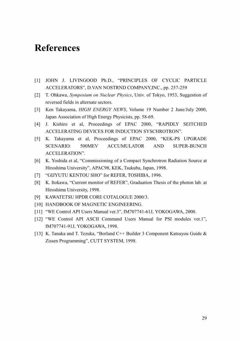
References

[1] JOHN J. LIVINGOOD Ph.D., “PRINCIPLES OF CYCLIC PARTICLE

ACCELERATORS”, D.VAN NOSTRND COMPANY,INC., pp. 257-259

[2] T. Ohkawa, Symposium on Nuclear Physics, Univ. of Tokyo, 1953, Suggestion of

reversed fields in alternate sectors.

[3] Ken Takayama, HIGH ENERGY NEWS, Volume 19 Number 2 June/July 2000,

Japan Association of High Energy Physicists, pp. 58-69.

[4] J. Kishiro et al, Proceedings of EPAC 2000, “RAPIDLY SEITCHED

ACCELERATING DEVICES FOR INDUCTION SYSCHROTRON”.

[5] K. Takayama et al, Proceedings of EPAC 2000, “KEK-PS UPGRADE

SCENARIO: 500MEV ACCUMULATOR AND SUPER-BUNCH

ACCELERATION”.

[6] K. Yoshida et al, “Commissioning of a Compact Synchrotron Radiation Source at

Hiroshima University”, APAC98, KEK, Tsukuba, Japan, 1998.

[7] “GIJYUTU KENTOU SHO” for REFER, TOSHIBA, 1996.

[8] K. Itokawa, “Current monitor of REFER”, Graduation Thesis of the photon lab. at

Hiroshima University, 1998.

[9] KAWATETSU HPDR CORE COTALOGUE 2000/3.

[10] HANDBOOK OF MAGNETIC ENGINEERING.

[11] “WE Control API Users Manual ver.3”, IM707741-61J, YOKOGAWA, 2000.

[12] “WE Control API ASCII Command Users Manual for PSI modules ver.1”,

IM707741-91J, YOKOGAWA, 1998.

[13] K. Tanaka and T. Tezuka, “Borland C++ Builder 3 Component Katsuyou Guide &

Zissen Programming”, CUTT SYSTEM, 1998.

30

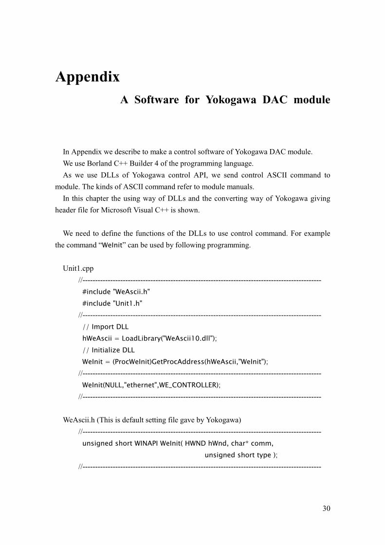
Appendix A Software for Yokogawa DAC module

In Appendix we describe to make a control software of Yokogawa DAC module.

We use Borland C++ Builder 4 of the programming language.

As we use DLLs of Yokogawa control API, we send control ASCII command to

module. The kinds of ASCII command refer to module manuals.

In this chapter the using way of DLLs and the converting way of Yokogawa giving

header file for Microsoft Visual C++ is shown.

We need to define the functions of the DLLs to use control command. For example

the command “WeInit” can be used by following programming.

Unit1.cpp

//-----------------------------------------------------------------------------------------------

#include "WeAscii.h" #include "Unit1.h"

//-----------------------------------------------------------------------------------------------

// Import DLL hWeAscii = LoadLibrary("WeAscii10.dll"); // Initialize DLL WeInit = (ProcWeInit)GetProcAddress(hWeAscii,"WeInit");

//-----------------------------------------------------------------------------------------------

WeInit(NULL,"ethernet",WE_CONTROLLER); //-----------------------------------------------------------------------------------------------

WeAscii.h (This is default setting file gave by Yokogawa) //-----------------------------------------------------------------------------------------------

unsigned short WINAPI WeInit( HWND hWnd, char* comm, unsigned short type );

//-----------------------------------------------------------------------------------------------

31

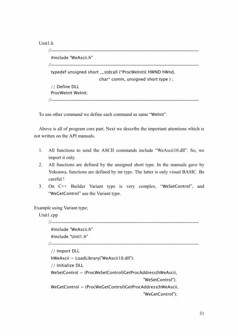
Unit1.h

//-----------------------------------------------------------------------------------------------

#include "WeAscii.h" //-----------------------------------------------------------------------------------------------

typedef unsigned short __stdcall (*ProcWeInit)( HWND hWnd, char* comm, unsigned short type ) ;

// Define DLL ProcWeInit WeInit;

//-----------------------------------------------------------------------------------------------

To use other command we define each command as same “WeInit”.

Above is all of program core part. Next we describe the important attentions which is

not written on the API manuals.

1. All functions to send the ASCII commands include “WeAscii10.dll”. So, we

import it only.

2. All functions are defined by the unsigned short type. In the manuals gave by

Yokoawa, functions are defined by int type. The latter is only visual BASIC. Be

careful !

3. On C++ Builder Variant type is very complex. “WeSetControl”, and

“WeGetControl” use the Variant type.

Example using Variant type;

Unit1.cpp

//-----------------------------------------------------------------------------------------------

#include "WeAscii.h" #include "Unit1.h"

//-----------------------------------------------------------------------------------------------

// Import DLL hWeAscii = LoadLibrary("WeAscii10.dll"); // Initialize DLL WeSetControl = (ProcWeSetControl)GetProcAddress(hWeAscii,

"WeSetControl"); WeGetControl = (ProcWeGetControl)GetProcAddress(hWeAscii,

"WeGetControl");

32

//-----------------------------------------------------------------------------------------------

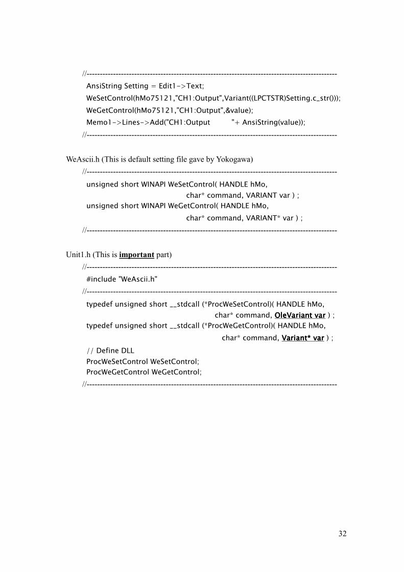
AnsiString Setting = Edit1->Text; WeSetControl(hMo75121,"CH1:Output",Variant((LPCTSTR)Setting.c_str())); WeGetControl(hMo75121,"CH1:Output",&value); Memo1->Lines->Add("CH1:Output の値 "+ AnsiString(value));

//-----------------------------------------------------------------------------------------------

WeAscii.h (This is default setting file gave by Yokogawa)

//-----------------------------------------------------------------------------------------------

unsigned short WINAPI WeSetControl( HANDLE hMo, char* command, VARIANT var ) ;

unsigned short WINAPI WeGetControl( HANDLE hMo, char* command, VARIANT* var ) ;

//-----------------------------------------------------------------------------------------------

Unit1.h (This is important part)

//-----------------------------------------------------------------------------------------------

#include "WeAscii.h" //-----------------------------------------------------------------------------------------------

typedef unsigned short __stdcall (*ProcWeSetControl)( HANDLE hMo, char* command, OleVariant varOleVariant varOleVariant varOleVariant var ) ;

typedef unsigned short __stdcall (*ProcWeGetControl)( HANDLE hMo, char* command, Variant* varVariant* varVariant* varVariant* var ) ;

// Define DLL ProcWeSetControl WeSetControl; ProcWeGetControl WeGetControl;

//-----------------------------------------------------------------------------------------------

Induction Acceleration for Beam-Orbit Control Seiji Matsuno

Department of Physics, Faculty of Science, Hiroshima University

Copyright © 2000-2001 by Seiji Matsuno

Serial Number Online PDF version / 15