INDUCTIVE AND UNSUPERVISED REPRESENTATION …

Published as a conference paper at ICLR 2020

INDUCTIVE AND UNSUPERVISED REPRESENTATIONLEARNING ON GRAPH STRUCTURED OBJECTS

Lichen Wang1, Bo Zong2, Qianqian Ma3, Wei Cheng2, Jingchao Ni2, Wenchao Yu2,Yanchi Liu2, Dongjin Song2, Haifeng Chen2, and Yun Fu1

1Northeastern University, Boston, USA2NEC Laboratories America, Princeton, USA3Boston University, Boston, [email protected], [email protected], [email protected],{bzong,weicheng,jni,wyu,yanchi,dsong,heifeng}@nec-labels.com

ABSTRACT

Inductive and unsupervised graph learning is a critical technique for predictiveor information retrieval tasks where label information is difficult to obtain. It isalso challenging to make graph learning inductive and unsupervised at the sametime, as learning processes guided by reconstruction error based loss functionsinevitably demand graph similarity evaluation that is usually computationally in-tractable. In this paper, we propose a general framework SEED (Sampling, Encod-ing, and Embedding Distributions) for inductive and unsupervised representationlearning on graph structured objects. Instead of directly dealing with the com-putational challenges raised by graph similarity evaluation, given an input graph,the SEED framework samples a number of subgraphs whose reconstruction errorscould be efficiently evaluated, encodes the subgraph samples into a collection ofsubgraph vectors, and employs the embedding of the subgraph vector distributionas the output vector representation for the input graph. By theoretical analysis,we demonstrate the close connection between SEED and graph isomorphism. Us-ing public benchmark datasets, our empirical study suggests the proposed SEEDframework is able to achieve up to 10% improvement, compared with competitivebaseline methods.

1 INTRODUCTION

Representation learning has been the core problem of machine learning tasks on graphs. Given agraph structured object, the goal is to represent the input graph as a dense low-dimensional vec-tor so that we are able to feed this vector into off-the-shelf machine learning or data manage-ment techniques for a wide spectrum of downstream tasks, such as classification (Niepert et al.,2016), anomaly detection (Akoglu et al., 2015), information retrieval (Li et al., 2019), and manyothers (Santoro et al., 2017b; Nickel et al., 2015).

In this paper, our work focuses on learning graph representations in an inductive and unsupervisedmanner. As inductive methods provide high efficiency and generalization for making inferenceover unseen data, they are desired in critical applications. For example, we could train a modelthat encodes graphs generated from computer program execution traces into vectors so that we canperform malware detection in a vector space. During real-time inference, efficient encoding and thecapability of processing unseen programs are expected for practical usage. Meanwhile, for real-lifeapplications where labels are expensive or difficult to obtain, such as anomaly detection (Zong et al.,2018) and information retrieval (Yan et al., 2005), unsupervised methods could provide effectivefeature representations shared among different tasks.

Inductive and unsupervised graph learning is challenging, even compared with its transductive orsupervised counterparts. First, when inductive capability is required, it is inevitable to deal with theproblem of node alignment such that we can discover common patterns across graphs. Second, inthe case of unsupervised learning, we have limited options to design objectives that guide learningprocesses. To evaluate the quality of the learned latent representations, reconstruction errors are

1


1 © NEC Corporation 2016 NEC Group Internal Use Only

Input GraphOutput Vector

RepresentationEmbedding Distribution Sampling Encoding

……

Encoding

space

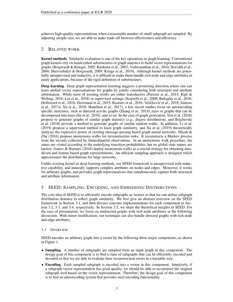
Figure 1: SEED consists of three components: sampling, encoding, and embedding distribution.Given an input graph, its vector representation can be obtained by going through the components.

commonly adopted. When node alignment meets reconstruction error, we have to answer a basicquestion: Given two graphs G1 and G2, are they identical or isomorphic (Chartrand, 1977)? To thisend, it could be computationally intractable to compute reconstruction errors (e.g., using graph editdistance (Zeng et al., 2009) as the metric) in order to capture detailed structural information.

Previous deep graph learning techniques mainly focus on transductive (Perozzi et al., 2014) or su-pervised settings (Li et al., 2019). A few recent studies focus on autoencoding specific structures,such as directed acyclic graphs (Zhang et al., 2019), trees or graphs that can be decomposed intotrees (Jin et al., 2018), and so on. From the perspective of graph generation, You et al. (2018) pro-pose to generate graphs of similar graph statistics (e.g., degree distribution), and Bojchevski et al.(2018) provide a GAN based method to generate graphs of similar random walks.

In this paper, we propose a general framework SEED (Sampling, Encoding, and Embedding Dis-tributions) for inductive and unsupervised representation learning on graph structured objects. Asshown in Figure 1, SEED consists of three major components: subgraph sampling, subgraph encod-ing, and embedding subgraph distributions. SEED takes arbitrary graphs as input, where nodes andedges could have rich features, or have no features at all. By sequentially going through the threecomponents, SEED outputs a vector representation for an input graph. One can further feed suchvector representations to off-the-shelf machine learning or data management tools for downstreamlearning or retrieval tasks.

Instead of directly addressing the computational challenge raised by evaluation of graph reconstruc-tion errors, SEED decomposes the reconstruction problem into the following two sub-problems.

Q1: How to efficiently autoencode and compare structural data in an unsupervised fashion? SEEDfocuses on a class of subgraphs whose encoding, decoding, and reconstruction errors can be eval-uated in polynomial time. In particular, we propose random walks with earliest visiting time(WEAVE) serving as the subgraph class, and utilize deep architectures to efficiently autoencodeWEAVEs. Note that reconstruction errors with respect to WEAVEs are evaluated in linear time.

Q2: How to measure the difference of two graphs in a tractable way? As one subgraph only coverspartial information of an input graph, SEED samples a number of subgraphs to enhance informationcoverage. With each subgraph encoded as a vector, an input graph is represented by a collectionof vectors. If two graphs are similar, their subgraph distribution will also be similar. Based on thisintuition, we evaluate graph similarity by computing distribution distance between two collectionsof vectors. By embedding distribution of subgraph representations, SEED outputs a vector repre-sentation for an input graph, where distance between two graphs’ vector representations reflects thedistance between their subgraph distributions.

Unlike existing message-passing based graph learning techniques whose expressive power is upperbounded by Weisfeiler-Lehman graph kernels (Xu et al., 2019; Shervashidze et al., 2011), we showthe direct relationship between SEED and graph isomorphism in Section 3.5.

We empirically evaluate the effectiveness of the SEED framework via classification and clusteringtasks on public benchmark datasets. We observe that graph representations generated by SEEDare able to effectively capture structural information, and maintain stable performance even whenthe node attributes are not available. Compared with competitive baseline methods, the proposedSEED framework could achieve up to 10% improvement in prediction accuracy. In addition, SEED

2


achieves high-quality representations when a reasonable number of small subgraph are sampled. Byadjusting sample size, we are able to make trade-off between effectiveness and efficiency.

2 RELATED WORK

Kernel methods. Similarity evaluation is one of the key operations in graph learning. Conventionalgraph kernels rely on handcrafted substructures or graph statistics to build vector representations forgraphs (Borgwardt & Kriegel, 2005; Kashima et al., 2003; Vishwanathan et al., 2010; Horvath et al.,2004; Shervashidze & Borgwardt, 2009; Kriege et al., 2019). Although kernel methods are poten-tially unsupervised and inductive, it is difficult to make them handle rich node and edge attributes inmany applications, because of the rigid definition of substructures.

Deep learning. Deep graph representation learning suggests a promising direction where one canlearn unified vector representations for graphs by jointly considering both structural and attributeinformation. While most of existing works are either transductive (Perozzi et al., 2014; Kipf &Welling, 2016; Liu et al., 2018) or supervised settings (Scarselli et al., 2008; Battaglia et al., 2016;Defferrard et al., 2016; Duvenaud et al., 2015; Kearnes et al., 2016; Velickovic et al., 2018; Santoroet al., 2017a; Xu et al., 2018; Hamilton et al., 2017), a few recent studies focus on autoencodingspecific structures, such as directed acyclic graphs (Zhang et al., 2019), trees or graphs that can bedecomposed into trees (Jin et al., 2018), and so on. In the case of graph generation, You et al. (2018)propose to generate graphs of similar graph statistics (e.g., degree distribution), and Bojchevskiet al. (2018) provide a method to generate graphs of similar random walks. In addition, Li et al.(2019) propose a supervised method to learn graph similarity, and Xu et al. (2019) theoreticallyanalyses the expressive power of existing message-passing based graph neural networks. Micali &Zhu (2016) propose anonymous walks for reconstruction tasks. It reconstructs a Markov processfrom the records collected by limited/partial observations. In an anonymous walk procedure, thestates are visited according to the underlying transition probabilities, but no global state names areknown. Ivanov & Burnaev (2018) deploy anonymous walks as a crucial strategy for obtaining data-driven and feature-based graph representations. An efficient sampling approach is designed whichapproximates the distributions for large networks.

Unlike existing kernel or deep learning methods, our SEED framework is unsupervised with induc-tive capability, and naturally supports complex attributes on nodes and edges. Moreover, it worksfor arbitrary graphs, and provides graph representations that simultaneously capture both structuraland attribute information.

3 SEED: SAMPLING, ENCODING, AND EMBEDDING DISTRIBUTIONS

The core idea of SEED is to efficiently encode subgraphs as vectors so that we can utilize subgraphdistribution distance to reflect graph similarity. We first give an abstract overview on the SEEDframework in Section 3.1, and then discuss concrete implementations for each component in Sec-tion 3.2, 3.3, and 3.4, respectively. In Section 3.5, we share the theoretical insights in SEED. Forthe ease of presentation, we focus on undirected graphs with rich node attributes in the followingdiscussion. With minor modification, our technique can also handle directed graphs with rich nodeand edge attributes.

3.1 OVERVIEW

SEED encodes an arbitrary graph into a vector by the following three major components, as shownin Figure 1.

• Sampling. A number of subgraphs are sampled from an input graph in this component. Thedesign goal of this component is to find a class of subgraphs that can be efficiently encoded anddecoded so that we are able to evaluate their reconstruction errors in a tractable way.

• Encoding. Each sampled subgraph is encoded into a vector in this component. Intuitively, ifa subgraph vector representation has good quality, we should be able to reconstruct the originalsubgraph well based on the vector representation. Therefore, the design goal of this componentis to find an autoencoding system that provides such encoding functionality.

3


• Embedding distribution. A collection of subgraph vector representations are aggregated intoone vector serving as the input graph’s representation. For two graphs, their distance in theoutput vector space approximates their subgraph distribution distance. The design goal of thiscomponent is to find such a aggregation function that preserves a pre-defined distribution distance.

Although there could be many possible implementations for the above three components, we proposea competitive implementation in this paper, and discuss them in details in the rest of this section.

3.2 SAMPLING


a

b b

aa

𝒢2

3 4

0 b-a-b-a-a-b

𝒃𝟎

-𝒂𝟏

-𝒃𝟎

-𝒂𝟑

-𝒂𝟒

-𝒃𝟎

1

ℋ

aa

b

a

0

13

4𝒃𝟎

-𝒂𝟏

-𝒃𝟐

-𝒂𝟑

-𝒂𝟒

-𝒃𝟎

b-a-b-a-a-b

WEAVE:

Vanilla

random walk:

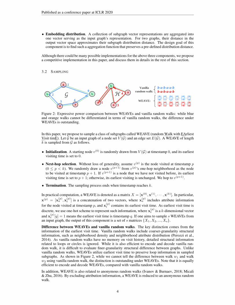
Figure 2: Expressive power comparison between WEAVEs and vanilla random walks: while blueand orange walks cannot be differentiated in terms of vanilla random walks, the difference underWEAVEs is outstanding.

In this paper, we propose to sample a class of subgraphs called WEAVE (random Walk with EArliestVisit timE). Let G be an input graph of a node set V (G) and an edge set E(G). A WEAVE of lengthk is sampled from G as follows.

• Initialization. A starting node v(0) is randomly drawn from V (G) at timestamp 0, and its earliestvisiting time is set to 0.

• Next-hop selection. Without loss of generality, assume v(p) is the node visited at timestamp p(0 ≤ p < k). We randomly draw a node v(p+1) from v(p)’s one-hop neighborhood as the nodeto be visited at timestamp p + 1. If v(p+1) is a node that we have not visited before, its earliestvisiting time is set to p+ 1; otherwise, its earliest visiting is unchanged. We hop to v(p+1).

• Termination. The sampling process ends when timestamp reaches k.

In practical computation, a WEAVE is denoted as a matrixX = [x(0),x(1), · · · ,x(k)]. In particular,x(p) = [x

(p)a ,x

(p)t ] is a concatenation of two vectors, where x

(p)a includes attribute information

for the node visited at timestamp p, and x(p)t contains its earliest visit time. As earliest visit time is

discrete, we use one-hot scheme to represent such information, where x(p)t is a k-dimensional vector

and x(p)t [q] = 1 means the earliest visit time is timestamp q. If one aims to sample s WEAVEs from

an input graph, the output of this component is a set of s matrices {X1, X2, ..., Xs}.Difference between WEAVEs and vanilla random walks. The key distinction comes from theinformation of the earliest visit time. Vanilla random walks include coarser-granularity structuralinformation, such as neighborhood density and neighborhood attribute distribution (Perozzi et al.,2014). As vanilla random walks have no memory on visit history, detailed structural informationrelated to loops or circles is ignored. While it is also efficient to encode and decode vanilla ran-dom walk, it is difficult to evaluate finer-granularity structural difference between graphs. Unlikevanilla random walks, WEAVEs utilize earliest visit time to preserve loop information in sampledsubgraphs. As shown in Figure 2, while we cannot tell the difference between walk w1 and walkw2 using vanilla random walk, the distinction is outstanding under WEAVEs. Note that it is equallyefficient to encode and decode WEAVEs, compared with vanilla random walks.

In addition, WEAVE is also related to anonymous random walks (Ivanov & Burnaev, 2018; Micali& Zhu, 2016). By excluding attribution information, a WEAVE is reduced to an anonymous randomwalk.

4


3.3 ENCODING

Given a set of sampled WEAVEs of length k {X1, X2, ..., Xs}, the goal is to encode each sam-pled WEAVE into a dense low-dimensional vector. As sampled WEAVEs share same length, theirmatrix representations also have identical shapes. Given a WEAVE X , one could encode it by anautoencoder (Hinton & Salakhutdinov, 2006) as follows.

z = f(X; θe), X = g(z; θd), (1)

where z is the dense low-dimensional representation for the input WEAVE, f(·) is the encodingfunction implemented by an MLP with parameters θe, and g(·) is the decoding function implementedby another MLP with parameters θd. The quality of z is evaluated through reconstruction errors asfollows,

L = ‖X − X‖22. (2)By conventional gradient descent based backpropagation (Kingma & Ba, 2014), one could optimizeθe and θd via minimizing reconstruction errorL. After such an autoencoder is well trained, the latentrepresentation z includes both node attribute information and finer-granularity structural informationsimultaneously. Given s sampled WEAVEs of an input graph, the output of this component is s denselow-dimensional vectors {z1, z2, · · · , zs}.

3.4 EMBEDDING DISTRIBUTION

Let G and H be two arbitrary graphs. Suppose subgraph (e.g., WEAVE) distributions for G andH are PG and PH, respectively. In this component, we are interested in evaluating the distancebetween PG and PH. In this work, we investigate the feasibility of employing empirical estimateof the maximum mean discrepancy (MMD) (Gretton et al., 2012) to evaluate subgraph distributiondistances, without assumptions on prior distributions, while there are multiple candidate metrics fordistribution distance evaluation, such as KL-divergence (Kullback & Leibler, 1951) and Wassersteindistance (Arjovsky et al., 2017). We leave the detailed comparison among different choices ofdistance metrics in our future work.

Given s subgraphs sampled from G as {z1, · · · , zs} and s subgraphs sampled from H as{h1, · · · ,hs}, we can estimate the distance between PG and PH under the MMD framework:

MMD(PG , PH) =1

s(s− 1)

s∑i=1

s∑j 6=i

k(zi, zj) +1

s(s− 1)

s∑i=1

s∑j 6=i

k(hi,hj)

− 2

s2

s∑i=1

s∑j=1

k(zi,hj)

=‖µG − µH‖22. (3)

µG and µH are empirical kernel embeddings of PG and PH, respectively, and are defined as follows,

µG =1

s

s∑i=1

φ(zi), µH =1

s

s∑i=1

φ(hi), (4)

where φ(·) is the implicit feature mapping function with respect to the kernel function k(·, ·). Tothis end, µG and µH are the output vector representation for G andH, respectively.

In terms of kernel selection, we find the following options are effective in practice.

Identity kernel. Under this kernel, pairwise similarity evaluation is performed in the original inputspace. Its implementation is simple, but surprisingly effective in real-life datasets,

µG =1

s

s∑i=1

zi, µH =1

s

s∑i=1

hi. (5)

where output representations are obtained by average aggregation over subgraph representations.

Commonly adopted kernels. For popular kernels (e.g., RBF kernel, inverse multi-quadratics ker-nel, and so on), it could be difficult to find and adopt their feature mapping functions. While approx-imation methods could be developed for individual kernels (Ring & Eskofier, 2016), we could train

5


a deep neural network that approximates such feature mapping functions. In particular,

µ′G =1

s

s∑i=1

φ(zi; θm), µ′H =1

s

s∑i=1

φ(hi; θm), D(PG , PH) = ‖µ′G − µ′H‖22, (6)

where φ(·; θm) is an MLP with parameters θm, and D(·, ·) is the approximation to the empiricalestimate of MMD. Note that µ′G and µ′H are output representations for G and H, respectively. Totrain the function φ(·; θm), we evaluate the approximation error by

J(θm) = ‖D(PG , PH)− MMD(PG , PH)‖22, (7)

where θm is optimized by minimizing J(θm).

3.5 THEORETICAL INSIGHTS

In this section, we sketch the theoretical connection between SEED and well-known graph isomor-phism (Chartrand, 1977), and show how walk length in WEAVE impacts the effectiveness in graphisomorphism tests. The full proof of theorems and lemmas is detailed in Appendix.

To make the discussion self-contained, we define graph isomorphism and its variant with node at-tributes as follows.

Graph isomorphism. G = (V (G), E(G)) and H = (V (H), E(H))) are isomorphic if there is abijection function f : V (G)⇔ V (H) such that ∀(u, v) ∈ E(G)⇔ (f(u), f(v)) ∈ E(H).Graph isomorphism with node attributes. Let G = (V (G), E(G), l1), H = (V (H), E(H), l2) betwo attributed graphs, where l1, l2 are attribute mapping functions l1 : V (G)→ Rd, l2 : V (H)→Rd, and node attributes are denoted as d-dimensional vectors. Then G and H are isomorphic withnode attributes if there is a bijection f : V (G) ⇔ V (H), s.t., ∀(u, v) ∈ E(G) ⇔ (f(u), f(v)) ∈E(H), and ∀u ∈ V (G), l1(u) = l2(f(u)).

Identical distributions. Two distributions P and Q are identical if and only if their 1st orderWasserstein distance (Ruschendorf, 1985) W1(P,Q) = 0.

The following theory suggests the minimum walk length for WEAVEs, if every edge in a graph isexpected to be visited.

Lemma 1. Let G = (V (G), E(G)) be a connected graph, then there exists a walk of length k whichcan visit all the edges of G, where k ≥ 2|E(G)| − 1.

Now, we are ready to present the connection between SEED and graph isomorphism.

Theorem 1. Let G = (V (G), E(G)) and H = (V (H), E(H)) be two connected graphs.Suppose we can enumerate all possible WEAVEs from G and H with a fixed-length k ≥2max{|E(G)|, |E(H)|}−1, where each WEAVE has a unique vector representation generated froma well-trained autoencoder. The Wasserstein distance between G’s and H’s WEAVE distributions is0 if and only if G andH are isomorphic.

The following theory shows the connection in the case of graphs with nodes attributes.

Theorem 2. Let G = (V (G), E(G)) and H = (V (H), E(H)) be two connected graphs with nodeattributes. Suppose we can enumerate all possible WEAVEs on G and H with a fixed-length k ≥2max{|E(G)|, |E(H)|}−1, where each WEAVE has a unique vector representation generated froma well-trained autoencoder. The Wasserstein distance between G’s and H’s WEAVE distributions is0 if and only if G andH are isomorphic with node attributes.

Note that similar results can be easily extended to the cases with both node and edge attributes, thecorresponding details can be found in Appendix E.

The theoretical results suggest the potential power of the SEED framework in capturing structuraldifference of graph data. As shown above, in order to achieve the same expressive power of graphisomorphism, we need to sample a large number of WEAVEs with a long walk length so that all pos-sible WEAVEs can be enumerated. The resource demand is impractical. However, in the empiricalstudy in Section 4, we show that SEED can achieve state-of-the-art performance, when we sample asmall number of WEAVEs with a reasonably short walk length.

6


4 EXPERIMENTS

4.1 DATASETS

We employ seven public benchmark datasets to evaluate the effectiveness of SEED. The brief intro-ductions of the datasets are listed below.

• Deezer User-User Friendship Networks (Deezer) (Rozemberczki et al., 2018) is a social net-work dataset which is collected from the music streaming service Deezer. It represents friendshipnetwork of users from three European countries (i.e., Romania, Croatia and Hungary). Thereare three graphs which corresponds to the three countries. Nodes represent the users and edgesare the mutual friendships. For the three graphs, the numbers of nodes are 41, 773, 54, 573, and47, 538, respectively, and the number of edges are 125, 826, 498, 202, and 222, 887, respectively.There exist 84 distinct genres, and genre notations are considered as node features. Thus, nodefeatures are represented as a 84-dimensional multi-hot vectors.

• Mutagenic Aromatic and Heteroaromatic Nitro Compounds (MUTAG) (Debnath et al., 1991)is a chemical bioinformatics dataset, which contains 188 chemical compounds. The compoundscan be divided into two classes according to their mutagenic effect on a bacterium. The chemicaldata can be converted to graph structures, where each node represents an atom. Explicit hydrogenatoms have been removed. In the obtained graph, the node attributes represent the atom types(i.e., C, N, O, F, I, Cl and Br) while the edge attributes represent bond types (i.e., single, double,triple or aromatic).

• NCI1 (Wale et al., 2008) represents a balanced subsets of datasets of chemical compoundsscreened for activity against non-small cell lung cancer and ovarian cancer cell lines, respec-tively. The label is assigned based on this characteristic. Each compound is converted to a graph.There are 4, 110 graphs in total with 122, 747 edges.

• PROTEINS (Borgwardt et al., 2005) is a bioinformatics dataset. The proteins in the datasetare converted to graphs based on the sub-structures and physical connections of the proteins.Specifically, nodes are secondary structure elements (SSEs), and edges represent the amino-acidsequence between the two neighbors. PROTEINS has 3 discrete labels (i.e., helix, sheet, andturn). There are 1, 113 graphs in total with 43, 471 edges.

• COLLAB (Leskovec et al., 2005) is a scientific collaboration dataset. It belongs to a socialconnection network in general. COLLAB is collected from 3 public collaboration datasets (i.e.,Astro Physics, Condensed Matter Physics, and High Energy Physics). The ego-networks aregenerated for individual researchers. The label of each graph represents the field which thisresearcher belongs to. There are 5, 000 graphs with 24, 574, 995 edges.

• IMDB-BINARY (Yanardag & Vishwanathan, 2015) is a collaboration dataset of film industry.The ego-network of each actor/actress is converted to a graph data. Each node represents anactor/actress and each edge is the indication if two actors/actresses if they appear in the samemovie. IMDB-BINARY has 1, 000 graphs associated with 19, 773 edges in total.

• IMDB-MULTI extends the IMDB-BINARY dataset to a multi-class version. It contains a bal-anced set of ego-networks derived from Sci-Fi, Romance, and Comedy genres. Specifically, thereare 1, 500 graphs with 19, 502 edges in total.

4.2 BASELINES

Three state-of-the-art representative techniques are implemented as baselines in the experiments.

• Graph Sample and Aggregate (GraphSAGE) (Hamilton et al., 2017) is an inductive graph rep-resentation learning approach in either supervised or unsupervised manner. GraphSAGE exploresnode and structure information by sampling and aggregating features from the local neighborhoodof each node. A forward propagation algorithm is specifically designed to aggregates the infor-mation together. We evaluate GraphSAGE in its unsupervised setting.

• Graph Matching Network (GMN) (Li et al., 2019) utilizes graph neural networks to obtaingraph representations for graph matching applications. A novel Graph Embedding Network isdesigned for better preserving node features and graph structures. In particular, Graph Matching

7


Network is proposed to directly obtain the similarity score of each pair of graphs. In our imple-mentation, we utilize the Graph Embedding Networks and deploy the graph-based loss functionproposed in (Hamilton et al., 2017) for unsupervised learning fashion.

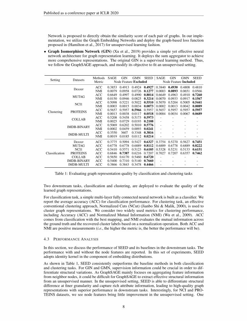
• Graph Isomorphism Network (GIN) (Xu et al., 2019) provides a simple yet effective neuralnetwork architecture for graph representation learning. It deploys the sum aggregator to achievemore comprehensive representations. The original GIN is a supervised learning method. Thus,we follow the GraphSAGE approach, and modify its objective to fit an unsupervised setting.

Setting Datasets Methods SAGE GIN GMN SEED SAGE GIN GMN SEEDMetric Node Feature Excluded Node Feature Included

Clustering

Dezzer ACC 0.3853 0.4913 0.4924 0.4927 0.3840 0.4930 0.4808 0.4810NMI 0.0079 0.0958 0.0726 0.1277 0.0003 0.0893 0.0651 0.0566

MUTAG ACC 0.6649 0.4997 0.4990 0.8014 0.6649 0.4963 0.4910 0.7260NMI 0.0150 0.0946 0.0825 0.3214 0.0070 0.0933 0.0917 0.1567

NCI1 ACC 0.5098 0.5221 0.5022 0.5510 0.5070 0.5204 0.5005 0.5441NMI 0.0003 0.0015 0.0034 0.0073 0.0002 0.0013 0.0042 0.0089

PROTEINS ACC 0.5657 0.5957 0.5966 0.5957 0.5657 0.5957 0.5957 0.5957NMI 0.0013 0.0038 0.0117 0.0518 0.0004 0.0034 0.0067 0.0689

COLLAB ACC 0.5208 0.5458 0.5173 0.5973 - - - -NMI 0.0025 0.0729 0.0193 0.2108 - - - -

IMDB-BINARY ACC 0.5069 0.6202 0.5010 0.5776 - - - -NMI 0.0002 0.0459 0.0093 0.0241 - - - -

IMDB-MULTI ACC 0.3550 3607 0.3348 0.3816 - - - -NMI 0.0019 0.0185 0.0112 0.0214 - - - -

Classification

Dezzer ACC 0.3775 0.5094 0.5427 0.6327 0.3754 0.5270 0.5627 0.7451MUTAG ACC 0.6778 0.6778 0.6889 0.8112 0.6889 0.6778 0.6889 0.8222

NCI1 ACC 0.5410 0.5571 0.5123 0.6105 0.5328 0.5231 0.5133 0.6151PROTEINS ACC 0.6846 0.7387 0.6216 0.7207 0.7027 0.7207 0.6357 0.7462COLLAB ACC 0.5650 0.6170 0.5460 0.6720 - - - -

IMDB-BINARY ACC 0.5400 0.7310 0.5140 0.7660 - - - -IMDB-MULTI ACC 0.3866 0.3843 0.3478 0.4466 - - - -

Table 1: Evaluating graph representation quality by classification and clustering tasks

Two downstream tasks, classification and clustering, are deployed to evaluate the quality of thelearned graph representations.

For classification task, a simple multi-layer fully connected neural network is built as a classifier. Wereport the average accuracy (ACC) for classification performance. For clustering task, an effectiveconventional clustering approach, Normalized Cuts (NCut) (Jianbo Shi & Malik, 2000), is used tocluster graph representations. We consider two widely used metrics for clustering performance,including Accuracy (ACC) and Normalized Mutual Information (NMI) (Wu et al., 2009). ACCcomes from classification with the best mapping, and NMI evaluates the mutual information acrossthe ground truth and the recovered cluster labels based on a normalization operation. Both ACC andNMI are positive measurements (i.e., the higher the metric is, the better the performance will be).

4.3 PERFORMANCE ANALYSIS

In this section, we discuss the performance of SEED and its baselines in the downstream tasks. Theperformance with and without the node features are reported. In this set of experiments, SEEDadopts identity kernel in the component of embedding distributions.

As shown in Table 1, SEED consistently outperforms the baseline methods in both classificationand clustering tasks. For GIN and GMN, supervision information could be crucial in order to dif-ferentiate structural variations. As GraphSAGE mainly focuses on aggregating feature informationfrom neighbor nodes, it could be difficult for GraphSAGE to extract effective structural informationfrom an unsupervised manner. In the unsupervised setting, SEED is able to differentiate structuraldifference at finer granularity and capture rich attribute information, leading to high-quality graphrepresentations with superior performance in downstream tasks. Interestingly, for NCI and PRO-TEINS datasets, we see node features bring little improvement in the unsupervised setting. One

8


possible reason could be node feature information has high correlation with structural informationin these cases.

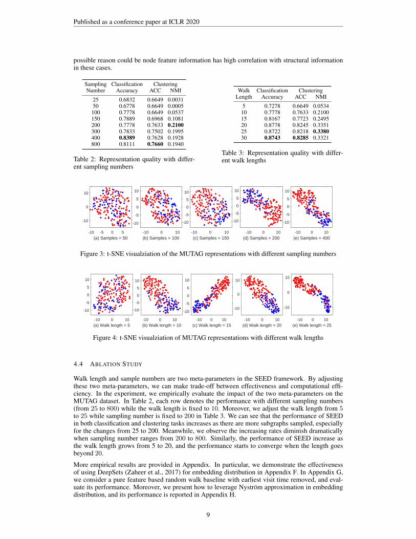
Sampling Classification ClusteringNumber Accuracy ACC NMI

25 0.6832 0.6649 0.003150 0.6778 0.6649 0.0005

100 0.7778 0.6649 0.0537150 0.7889 0.6968 0.1081200 0.7778 0.7633 0.2100300 0.7833 0.7502 0.1995400 0.8389 0.7628 0.1928800 0.8111 0.7660 0.1940

Table 2: Representation quality with differ-ent sampling numbers

Walk Classification ClusteringLength Accuracy ACC NMI

5 0.7278 0.6649 0.053410 0.7778 0.7633 0.210015 0.8167 0.7723 0.249520 0.8778 0.8245 0.335125 0.8722 0.8218 0.338030 0.8743 0.8285 0.3321

Table 3: Representation quality with differ-ent walk lengths

-10 -5 0 5

(a) Samples = 50

-10

0

10

-10 0 10

(b) Samples = 100

-10

-5

0

5

10

-10 0 10

(c) Samples = 150

-10

-5

0

5

10

-10 0 10

(d) Samples = 200

-10

-5

0

5

10

-10 0 10

(e) Samples = 400

-10

-5

0

5

10

Figure 3: t-SNE visualziation of the MUTAG representations with different sampling numbers

-10 0 10

(a) Walk length = 5

-10

-5

0

5

10

-10 0 10

(b) Walk length = 10

-10

-5

0

5

10

-10 0 10

(c) Walk length = 15

-10

-5

0

5

10

-10 0 10

(d) Walk length = 20

-10

0

10

-10 0 10

(e) Walk length = 25

-10

0

10

Figure 4: t-SNE visualziation of MUTAG representations with different walk lengths

4.4 ABLATION STUDY

Walk length and sample numbers are two meta-parameters in the SEED framework. By adjustingthese two meta-parameters, we can make trade-off between effectiveness and computational effi-ciency. In the experiment, we empirically evaluate the impact of the two meta-parameters on theMUTAG dataset. In Table 2, each row denotes the performance with different sampling numbers(from 25 to 800) while the walk length is fixed to 10. Moreover, we adjust the walk length from 5to 25 while sampling number is fixed to 200 in Table 3. We can see that the performance of SEEDin both classification and clustering tasks increases as there are more subgraphs sampled, especiallyfor the changes from 25 to 200. Meanwhile, we observe the increasing rates diminish dramaticallywhen sampling number ranges from 200 to 800. Similarly, the performance of SEED increase asthe walk length grows from 5 to 20, and the performance starts to converge when the length goesbeyond 20.

More empirical results are provided in Appendix. In particular, we demonstrate the effectivenessof using DeepSets (Zaheer et al., 2017) for embedding distribution in Appendix F. In Appendix G,we consider a pure feature based random walk baseline with earliest visit time removed, and eval-uate its performance. Moreover, we present how to leverage Nystrom approximation in embeddingdistribution, and its performance is reported in Appendix H.

9


-10 -5 0 5 10(a) Identity Kernel

-10

-5

0

5

10

-10 -5 0 5 10

-10

-5

0

5

10

(b) RBF Kernel

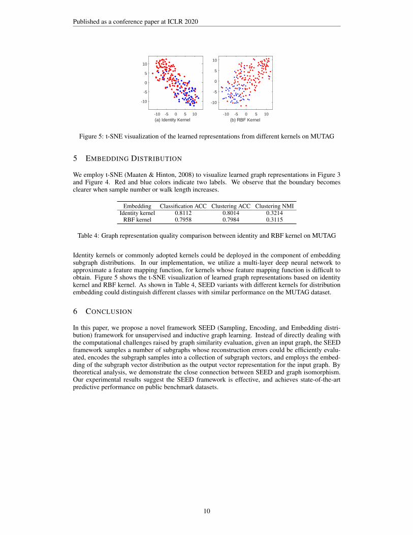
Figure 5: t-SNE visualization of the learned representations from different kernels on MUTAG

5 EMBEDDING DISTRIBUTION

We employ t-SNE (Maaten & Hinton, 2008) to visualize learned graph representations in Figure 3and Figure 4. Red and blue colors indicate two labels. We observe that the boundary becomesclearer when sample number or walk length increases.

Embedding Classification ACC Clustering ACC Clustering NMIIdentity kernel 0.8112 0.8014 0.3214

RBF kernel 0.7958 0.7984 0.3115

Table 4: Graph representation quality comparison between identity and RBF kernel on MUTAG

Identity kernels or commonly adopted kernels could be deployed in the component of embeddingsubgraph distributions. In our implementation, we utilize a multi-layer deep neural network toapproximate a feature mapping function, for kernels whose feature mapping function is difficult toobtain. Figure 5 shows the t-SNE visualization of learned graph representations based on identitykernel and RBF kernel. As shown in Table 4, SEED variants with different kernels for distributionembedding could distinguish different classes with similar performance on the MUTAG dataset.

6 CONCLUSION

In this paper, we propose a novel framework SEED (Sampling, Encoding, and Embedding distri-bution) framework for unsupervised and inductive graph learning. Instead of directly dealing withthe computational challenges raised by graph similarity evaluation, given an input graph, the SEEDframework samples a number of subgraphs whose reconstruction errors could be efficiently evalu-ated, encodes the subgraph samples into a collection of subgraph vectors, and employs the embed-ding of the subgraph vector distribution as the output vector representation for the input graph. Bytheoretical analysis, we demonstrate the close connection between SEED and graph isomorphism.Our experimental results suggest the SEED framework is effective, and achieves state-of-the-artpredictive performance on public benchmark datasets.

10


REFERENCES

Leman Akoglu, Hanghang Tong, and Danai Koutra. Graph based anomaly detection and description:a survey. Data mining and knowledge discovery, 29(3):626–688, 2015.

Martin Arjovsky, Soumith Chintala, and Leon Bottou. Wasserstein gan. arXiv preprintarXiv:1701.07875, 2017.

Peter Battaglia, Razvan Pascanu, Matthew Lai, Danilo Jimenez Rezende, et al. Interaction net-works for learning about objects, relations and physics. In Proceedings of Advances in neuralinformation processing systems, pp. 4502–4510, 2016.

Aleksandar Bojchevski, Oleksandr Shchur, Daniel Zugner, and Stephan Gunnemann. Netgan: Gen-erating graphs via random walks. In Proceedings of International Conference on Machine Learn-ing, 2018.

Karsten M Borgwardt and Hans-Peter Kriegel. Shortest-path kernels on graphs. In Proceedings ofIEEE International conference on data mining, pp. 8–pp, 2005.

Karsten M Borgwardt, Cheng Soon Ong, Stefan Schonauer, SVN Vishwanathan, Alex J Smola, andHans-Peter Kriegel. Protein function prediction via graph kernels. Bioinformatics, 21(suppl 1):i47–i56, 2005.

Gary Chartrand. Introductory graph theory. Courier Corporation, 1977.

Asim Kumar Debnath, Rosa L Lopez de Compadre, Gargi Debnath, Alan J Shusterman, and Cor-win Hansch. Structure-activity relationship of mutagenic aromatic and heteroaromatic nitro com-pounds. correlation with molecular orbital energies and hydrophobicity. Journal of medicinalchemistry, 34(2):786–797, 1991.

Michael Defferrard, Xavier Bresson, and Pierre Vandergheynst. Convolutional neural networks ongraphs with fast localized spectral filtering. In Proceedings of Advances in neural informationprocessing systems, pp. 3844–3852, 2016.

David K Duvenaud, Dougal Maclaurin, Jorge Iparraguirre, Rafael Bombarell, Timothy Hirzel, AlanAspuru-Guzik, and Ryan P Adams. Convolutional networks on graphs for learning molecularfingerprints. In Proceedings of Advances in neural information processing systems, pp. 2224–2232, 2015.

Arthur Gretton, Karsten M Borgwardt, Malte J Rasch, Bernhard Scholkopf, and Alexander Smola.A kernel two-sample test. Journal of Machine Learning Research, 13(Mar):723–773, 2012.

Will Hamilton, Zhitao Ying, and Jure Leskovec. Inductive representation learning on large graphs.In Proceedings of Advances in Neural Information Processing Systems, pp. 1024–1034, 2017.

Geoffrey E Hinton and Ruslan R Salakhutdinov. Reducing the dimensionality of data with neuralnetworks. science, 313(5786):504–507, 2006.

Tamas Horvath, Thomas Gartner, and Stefan Wrobel. Cyclic pattern kernels for predictive graphmining. In Proceedings of ACM SIGKDD international conference on Knowledge discovery anddata mining, pp. 158–167, 2004.

Sergey Ivanov and Evgeny Burnaev. Anonymous walk embeddings. In Jennifer Dy and AndreasKrause (eds.), Proceedings of International Conference on Machine Learning, volume 80 of Pro-ceedings of Machine Learning Research, pp. 2186–2195, Stockholmsmassan, Stockholm Swe-den, 10–15 Jul 2018. PMLR.

Jianbo Shi and J. Malik. Normalized cuts and image segmentation. IEEE Transactions on PatternAnalysis and Machine Intelligence, 22(8):888–905, Aug 2000.

Wengong Jin, Regina Barzilay, and Tommi Jaakkola. Junction tree variational autoencoder formolecular graph generation. In Proceedings of International Conference on Machine Learning,2018.

11


Hisashi Kashima, Koji Tsuda, and Akihiro Inokuchi. Marginalized kernels between labeled graphs.In Proceedings of International conference on machine learning (ICML-03), pp. 321–328, 2003.

Steven Kearnes, Kevin McCloskey, Marc Berndl, Vijay Pande, and Patrick Riley. Molecular graphconvolutions: moving beyond fingerprints. Journal of computer-aided molecular design, 30(8):595–608, 2016.

Diederik P Kingma and Jimmy Ba. Adam: A method for stochastic optimization. arXiv preprintarXiv:1412.6980, 2014.

Thomas N Kipf and Max Welling. Variational graph auto-encoders. arXiv preprintarXiv:1611.07308, 2016.

Nils M. Kriege, Fredrik D. Johansson, and Christopher Morris. A survey on graph kernels. CoRR,abs/1903.11835, 2019. URL http://arxiv.org/abs/1903.11835.

Solomon Kullback and Richard A Leibler. On information and sufficiency. The annals of mathe-matical statistics, 22(1):79–86, 1951.

Jure Leskovec, Jon Kleinberg, and Christos Faloutsos. Graphs over time: densification laws, shrink-ing diameters and possible explanations. In Proceedings of the eleventh ACM SIGKDD interna-tional conference on Knowledge discovery in data mining, pp. 177–187. ACM, 2005.

Yujia Li, Chenjie Gu, Thomas Dullien, Oriol Vinyals, and Pushmeet Kohli. Graph matching net-works for learning the similarity of graph structured objects. In Kamalika Chaudhuri and RuslanSalakhutdinov (eds.), Proceedings of International Conference on Machine Learning, volume 97,pp. 3835–3845, 09–15 Jun 2019.

Qi Liu, Miltiadis Allamanis, Marc Brockschmidt, and Alexander Gaunt. Constrained graph vari-ational autoencoders for molecule design. In Proceedings of Advances in Neural InformationProcessing Systems, pp. 7795–7804, 2018.

Laurens van der Maaten and Geoffrey Hinton. Visualizing data using t-SNE. Journal of machinelearning research, 9(Nov):2579–2605, 2008.

Silvio Micali and Zeyuan Allen Zhu. Reconstructing markov processes from independent andanonymous experiments. Discrete Applied Mathematics, 200:108–122, 2016.

Maximilian Nickel, Kevin Murphy, Volker Tresp, and Evgeniy Gabrilovich. A review of relationalmachine learning for knowledge graphs. Proceedings of IEEE, 104(1):11–33, 2015.

Mathias Niepert, Mohamed Ahmed, and Konstantin Kutzkov. Learning convolutional neural net-works for graphs. In Proceedings of International Conference on Machine Learning, pp. 2014–2023, 2016.

Bryan Perozzi, Rami Al-Rfou, and Steven Skiena. Deepwalk: Online learning of social representa-tions. In Proceedings of ACM SIGKDD International Conference on Knowledge Discovery andData Mining, pp. 701–710. ACM, 2014.

Matthias Ring and Bjoern M Eskofier. An approximation of the gaussian rbf kernel for efficientclassification with svms. Pattern Recognition Letters, 84:107–113, 2016.

Benedek Rozemberczki, Ryan Davies, Rik Sarkar, and Charles Sutton. Gemsec: Graph embeddingwith self clustering. arXiv preprint arXiv:1802.03997, 2018.

Ludger Ruschendorf. The wasserstein distance and approximation theorems. Probability Theoryand Related Fields, 70(1):117–129, 1985.

Adam Santoro, David Raposo, David G Barrett, Mateusz Malinowski, Razvan Pascanu, PeterBattaglia, and Timothy Lillicrap. A simple neural network module for relational reasoning. InProceedings of Advances in neural information processing systems, pp. 4967–4976, 2017a.

Adam Santoro, David Raposo, David G Barrett, Mateusz Malinowski, Razvan Pascanu, PeterBattaglia, and Timothy Lillicrap. A simple neural network module for relational reasoning. InProceedings of Advances in neural information processing systems, pp. 4967–4976, 2017b.

12

http://arxiv.org/abs/1903.11835


Franco Scarselli, Marco Gori, Ah Chung Tsoi, Markus Hagenbuchner, and Gabriele Monfardini.The graph neural network model. IEEE Transactions on Neural Networks, 20(1):61–80, 2008.

Nino Shervashidze and Karsten Borgwardt. Fast subtree kernels on graphs. In Proceedings ofAdvances in neural information processing systems, pp. 1660–1668, 2009.

Nino Shervashidze, Pascal Schweitzer, Erik Jan van Leeuwen, Kurt Mehlhorn, and Karsten M Borg-wardt. Weisfeiler-lehman graph kernels. Journal of Machine Learning Research, 12(Sep):2539–2561, 2011.

Petar Velickovic, Guillem Cucurull, Arantxa Casanova, Adriana Romero, Pietro Lio, and YoshuaBengio. Graph attention networks. In Proceedings of International Conference on LearningRepresentations, 2018.

S Vichy N Vishwanathan, Nicol N Schraudolph, Risi Kondor, and Karsten M Borgwardt. Graphkernels. Journal of Machine Learning Research, 11(Apr):1201–1242, 2010.

Nikil Wale, Ian A Watson, and George Karypis. Comparison of descriptor spaces for chemical com-pound retrieval and classification. Knowledge and Information Systems, 14(3):347–375, 2008.

Christopher KI Williams and Matthias Seeger. Using the nystrom method to speed up kernel ma-chines. In Advances in neural information processing systems, pp. 682–688, 2001.

Junjie Wu, Hui Xiong, and Jian Chen. Adapting the right measures for k-means clustering. InProceedings of the ACM SIGKDD international conference on Knowledge discovery and datamining, pp. 877–886, 2009.

Keyulu Xu, Chengtao Li, Yonglong Tian, Tomohiro Sonobe, Ken ichi Kawarabayashi, and StefanieJegelka. Representation learning on graphs with jumping knowledge networks. In Proceedingsof International Conference on Machine Learning, 2018.

Keyulu Xu, Weihua Hu, Jure Leskovec, and Stefanie Jegelka. How powerful are graph neuralnetworks? In Proceedings of International Conference on Learning Representations, 2019.

Xifeng Yan, Philip S Yu, and Jiawei Han. Substructure similarity search in graph databases. InProceedings of ACM SIGMOD international conference on Management of data, pp. 766–777.ACM, 2005.

Pinar Yanardag and SVN Vishwanathan. Deep graph kernels. In Proceedings of the ACM SIGKDDInternational Conference on Knowledge Discovery and Data Mining, pp. 1365–1374. ACM,2015.

Jiaxuan You, Rex Ying, Xiang Ren, William L Hamilton, and Jure Leskovec. Graphrnn: Generatingrealistic graphs with deep auto-regressive models. In Proceedings of International Conference onMachine Learning, 2018.

Manzil Zaheer, Satwik Kottur, Siamak Ravanbakhsh, Barnabas Poczos, Ruslan R Salakhutdinov,and Alexander J Smola. Deep sets. In Advances in neural information processing systems, pp.3391–3401, 2017.

Zhiping Zeng, Anthony KH Tung, Jianyong Wang, Jianhua Feng, and Lizhu Zhou. Comparing stars:On approximating graph edit distance. Proceedings of VLDB Endowment, 2(1):25–36, 2009.

Muhan Zhang, Shali Jiang, Zhicheng Cui, Roman Garnett, and Yixin Chen. D-vae: A variationalautoencoder for directed acyclic graphs. arXiv preprint arXiv:1904.11088, 2019.

Bo Zong, Qi Song, Martin Renqiang Min, Wei Cheng, Cristian Lumezanu, Daeki Cho, and HaifengChen. Deep autoencoding gaussian mixture model for unsupervised anomaly detection. In Pro-ceedings of International Conference on Learning Representations, 2018.

13


A PROOF FOR LEMMA 1

Proof. We will use induction on |E(G)| to complete the proof.

Basic case: Let |E(G)| = 1, the only possible graph is a line graph of length 1. For such a graph, thewalk from one node to another can cover the only edge on the graph, which has length 1 = 2 · 1− 1.

Induction: We assume for all the connected graphs on less than m edges (i.e., |E(G)| ≤ m − 1),there exist a walk of length k which can visit all the edges if k ≥ 2|E(G)| − 1. Then we will showfor any connected graph with m edges, there also exists a walk which can cover all the edges on thegraph with length k ≥ 2|E(G)| − 1.

Let G = (V (G), E(G)) be a connected graph with |E(G)| = m. Firstly, we assume G is not a tree,which means there exist a cycle on G. By removing an edge e = (vi, vj) from the cycle, we canget a graph G′ on m − 1 edges which is still connected. This is because any edge on a cycle is notbridge. Then according to the induction hypothesis, there exists a walk w′ = v1v2 . . . vi . . . vj . . . vtof length k′ ≥ 2(m− 1)+ 1 which can visit all the edges on G′ (The walk does not necessarily startfrom node 1, v1 just represents the first node appears in this walk). Next, we will go back to ourgraph G, as G′ is a subgraph of G, w′ is also a walk on G. By replacing the first appeared node vi onwalk w′ with a walk vivjvi, we can obtain a new walk w = v1v2 . . . vivjvi . . . vj . . . vt on G. As wcan cover all the edges on G′ and the edge e with length k = k′+2 ≥ 2(m− 1)− 1+ 2 = 2m− 1,which means it can cover all the edges on G with length k ≥ 2|E(G)| − 1.

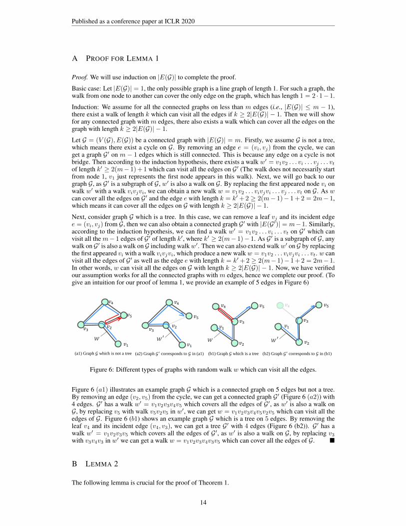
Next, consider graph G which is a tree. In this case, we can remove a leaf vj and its incident edgee = (vi, vj) from G, then we can also obtain a connected graph G′ with |E(G′)| = m−1. Similarly,according to the induction hypothesis, we can find a walk w′ = v1v2 . . . vi . . . vt on G′ which canvisit all the m− 1 edges of G′ of length k′, where k′ ≥ 2(m− 1)− 1. As G′ is a subgraph of G, anywalk on G′ is also a walk on G including walkw′. Then we can also extend walkw′ on G by replacingthe first appeared vi with a walk vivjvi, which produce a new walkw = v1v2 . . . vivjvi . . . vt. w canvisit all the edges of G′ as well as the edge e with length k = k′+2 ≥ 2(m− 1)− 1+2 = 2m− 1.In other words, w can visit all the edges on G with length k ≥ 2|E(G)| − 1. Now, we have verifiedour assumption works for all the connected graphs with m edges, hence we complete our proof. (Togive an intuition for our proof of lemma 1, we provide an example of 5 edges in Figure 6)


Walk length analysis

(a2) Graph 𝒢′ corresponds to 𝒢 in (a1)

𝑣3

(b1) Graph 𝒢 which is a tree

𝑣1

(a1) Graph 𝒢 which is not a tree

𝑣1

𝑣4

𝑣5

𝑣2

(b2) Graph 𝒢′ corresponds to 𝒢 in (b1)

𝑣2

𝑣5

𝑣3

𝑣4

𝑣3

𝑣1

𝑣4

𝑣5

𝑣2 𝑣1

𝑣2

𝑣5

𝑣3

𝑣4

𝑤′𝑤 𝑤′𝑤

Figure 6: Different types of graphs with random walk w which can visit all the edges.

Figure 6 (a1) illustrates an example graph G which is a connected graph on 5 edges but not a tree.By removing an edge (v2, v5) from the cycle, we can get a connected graph G′ (Figure 6 (a2)) with4 edges. G′ has a walk w′ = v1v2v3v4v5 which covers all the edges of G′, as w′ is also a walk onG, by replacing v5 with walk v5v2v5 in w′, we can get w = v1v2v3v4v5v2v5 which can visit all theedges of G. Figure 6 (b1) shows an example graph G which is a tree on 5 edges. By removing theleaf v4 and its incident edge (v4, v3), we can get a tree G′ with 4 edges (Figure 6 (b2)). G′ has awalk w′ = v1v2v3v5 which covers all the edges of G′, as w′ is also a walk on G, by replacing v3with v3v4v3 in w′ we can get a walk w = v1v2v3v4v3v5 which can cover all the edges of G. �

B LEMMA 2

The following lemma is crucial for the proof of Theorem 1.

14


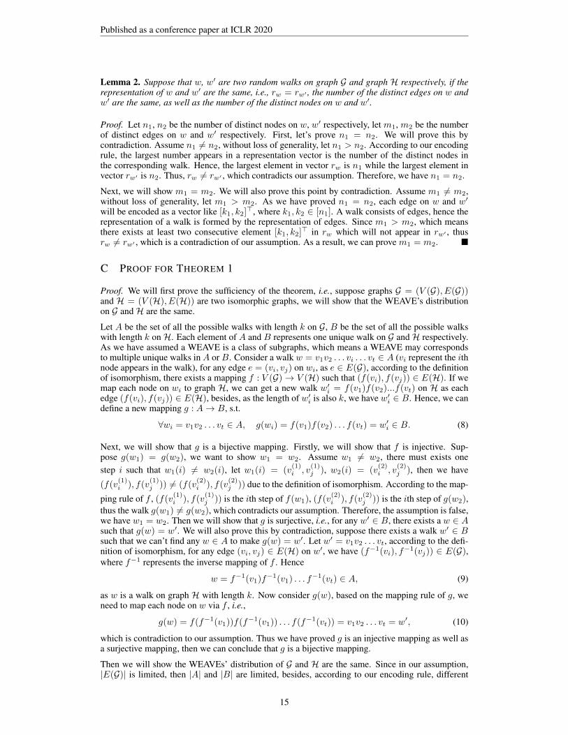
Lemma 2. Suppose that w, w′ are two random walks on graph G and graph H respectively, if therepresentation of w and w′ are the same, i.e., rw = rw′ , the number of the distinct edges on w andw′ are the same, as well as the number of the distinct nodes on w and w′.

Proof. Let n1, n2 be the number of distinct nodes on w, w′ respectively, let m1, m2 be the numberof distinct edges on w and w′ respectively. First, let’s prove n1 = n2. We will prove this bycontradiction. Assume n1 6= n2, without loss of generality, let n1 > n2. According to our encodingrule, the largest number appears in a representation vector is the number of the distinct nodes inthe corresponding walk. Hence, the largest element in vector rw is n1 while the largest element invector rw′ is n2. Thus, rw 6= rw′ , which contradicts our assumption. Therefore, we have n1 = n2.

Next, we will show m1 = m2. We will also prove this point by contradiction. Assume m1 6= m2,without loss of generality, let m1 > m2. As we have proved n1 = n2, each edge on w and w′will be encoded as a vector like [k1, k2]

>, where k1, k2 ∈ [n1]. A walk consists of edges, hence therepresentation of a walk is formed by the representation of edges. Since m1 > m2, which meansthere exists at least two consecutive element [k1, k2]> in rw which will not appear in rw′ , thusrw 6= rw′ , which is a contradiction of our assumption. As a result, we can prove m1 = m2. �

C PROOF FOR THEOREM 1

Proof. We will first prove the sufficiency of the theorem, i.e., suppose graphs G = (V (G), E(G))and H = (V (H), E(H)) are two isomorphic graphs, we will show that the WEAVE’s distributionon G andH are the same.

Let A be the set of all the possible walks with length k on G, B be the set of all the possible walkswith length k onH. Each element of A and B represents one unique walk on G andH respectively.As we have assumed a WEAVE is a class of subgraphs, which means a WEAVE may correspondsto multiple unique walks in A orB. Consider a walk w = v1v2 . . . vi . . . vt ∈ A (vi represent the ithnode appears in the walk), for any edge e = (vi, vj) on wi, as e ∈ E(G), according to the definitionof isomorphism, there exists a mapping f : V (G)→ V (H) such that (f(vi), f(vj)) ∈ E(H). If wemap each node on wi to graph H, we can get a new walk w′i = f(v1)f(v2)...f(vt) on H as eachedge (f(vi), f(vj)) ∈ E(H), besides, as the length of w′i is also k, we have w′i ∈ B. Hence, we candefine a new mapping g : A→ B, s.t.

∀wi = v1v2 . . . vt ∈ A, g(wi) = f(v1)f(v2) . . . f(vt) = w′i ∈ B. (8)

Next, we will show that g is a bijective mapping. Firstly, we will show that f is injective. Sup-pose g(w1) = g(w2), we want to show w1 = w2. Assume w1 6= w2, there must exists onestep i such that w1(i) 6= w2(i), let w1(i) = (v

(1)i , v

(1)j ), w2(i) = (v

(2)i , v

(2)j ), then we have

(f(v(1)i ), f(v

(1)j )) 6= (f(v

(2)i ), f(v

(2)j )) due to the definition of isomorphism. According to the map-

ping rule of f , (f(v(1)i ), f(v(1)j )) is the ith step of f(w1), (f(v

(2)i ), f(v

(2)j )) is the ith step of g(w2),

thus the walk g(w1) 6= g(w2), which contradicts our assumption. Therefore, the assumption is false,we have w1 = w2. Then we will show that g is surjective, i.e., for any w′ ∈ B, there exists a w ∈ Asuch that g(w) = w′. We will also prove this by contradiction, suppose there exists a walk w′ ∈ Bsuch that we can’t find any w ∈ A to make g(w) = w′. Let w′ = v1v2 . . . vt, according to the defi-nition of isomorphism, for any edge (vi, vj) ∈ E(H) on w′, we have (f−1(vi), f

−1(vj)) ∈ E(G),where f−1 represents the inverse mapping of f . Hence

w = f−1(v1)f−1(v1) . . . f

−1(vt) ∈ A, (9)

as w is a walk on graph H with length k. Now consider g(w), based on the mapping rule of g, weneed to map each node on w via f , i.e.,

g(w) = f(f−1(v1))f(f−1(v1)) . . . f(f

−1(vt)) = v1v2 . . . vt = w′, (10)

which is contradiction to our assumption. Thus we have proved g is an injective mapping as well asa surjective mapping, then we can conclude that g is a bijective mapping.

Then we will show the WEAVEs’ distribution of G and H are the same. Since in our assumption,|E(G)| is limited, then |A| and |B| are limited, besides, according to our encoding rule, different

15


walks may correspond to one specific WEAVE while each WEAVE corresponds a unique represen-tation vector, thus the number of all the possible representation vectors is limited for both G and H.Thus, the representation vector’s distributions PG for graph G and representation’s distributions PHfor graph H are both discrete distributions. To compare the similarity of two discrete probabilitydistributions, we can adopt the following equation to compute the Wasserstein distance and check ifit is 0.

W1(P,Q) =minπ

m∑i=1

n∑j=1

π(i, j)s(i, j),

s.t.m∑i=1

π(i, j) = wqj ,∀j,

n∑j=1

π(i, j) = wpi ,∀i,

π(i, j) ≥ 0,∀i, j,

(11)

where W1(P,Q) is the Wasserstein distance of probability distribution P and Q, π(i, j) is the costfunction and s(i, j) is a distance function,wqj andwpj are the probabilities of qj and pj respectively.

Since we have proved g : A → B is a bijection, besides, according to our encoding rule, g(w) andw will corresponds to the same WEAVE, hence they will share the same representation vector. Asa consequence, for each point (gi, wgi) (gi corresponds to a representation vector, wgi representsthe probability of gi) in the distribution PG , we can find a point (hi, whi

) in PH such that gi =hi, and wgi = whi . Then consider (11), for PG and PH, if we let π be a diagonal matrix with[wp1 , wp2 , . . . , wpm ] on the diagonal and all the other elements be 0, we can make each element inthe sum

∑mi=1

∑nj=1 π(i, j)s(i, j) be 0, as this sum is supposed to be nonnegative, its minimum

is 0, hence W1(PG , PH) = 0, which means for two isomorphic graphs G and H, their WEAVE’sdistributions PG and PH are the same.

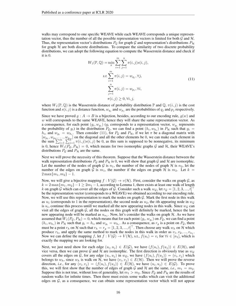
Next we will prove the necessity of this theorem. Suppose that the Wasserstein distance between thewalk representation distributions PG and PH is 0, we will show that graph G andH are isomorphic.Let the number of the nodes of graph G is n1, the number of the nodes of graph H is n2, let thenumber of the edges on graph G is m1, the number if the edges on graph H is m2. Let k =2max{m1,m2} − 1.

Now, we will give a bijective mapping f : V (G) → v(H). First, consider the walks on graph G, ask = 2max{m1,m2}−1 ≥ 2m1−1, according to Lemma 1, there exists at least one walk of lengthk on graph G which can cover all the edges of G. Consider such a walk wG , let rG = [1, 2, 3, ..., t]>

be the representation vector (corresponds to a WEAVE) we obtained according to our encoding rule.Now, we will use this representation to mark the nodes on graph G. Mark the first node in this walkas u1 (corresponds to 1 in the representation), the second node as u2, the ith appearing node in wGis ui, continue this process untill we marked all the new appearing nodes in this walk. Since wG canvisit all the edges of graph G, all the nodes on this graph will definitely be marked, hence the lastnew appearing node will be marked as un1

. Now, let’s consider the walks on graph H. As we haveassumed thatW1(PG , PH) = 0, which means that for each point (gi, wgi) on PG , we can find a point(hi, whi

) in PH such that gi = hi, and wgi = whi. As a consequence, as rg is a point on PG , there

must be a point rh onH such that rh = rg = [1, 2, 3, ..., t]>. Then choose any walk wh onH whichproduce rh, and apply the same method to mark the nodes in this walk in order as v1, v2, ..., vn1

.Now we can define the mapping f , let f : V (G) → V (H), s.t., f(ui) = vi for ∀i ∈ [n1], which isexactly the mapping we are looking for.

Next, we just need show for each edge (ui, uj) ∈ E(G), we have (f(ui), f(uj)) ∈ E(H), andvice versa, then we can prove G and H are isomorphic. The first direction is obviously true as wGcovers all the edges on G, for any edge (ui, uj) in wG , we have (f(ui), f(uj)) = (vi, vj) whichbelongs to wh, since wh is walk on H, we have (vi, vj) ∈ E(H). Then we will prove the reversedirection, i.e., for any (vi, vj) = (f(ui), f(uj)) ∈ E(H), we have (ui, uj) ∈ E(G). To provethis, we will first show that the number of edges of graph G and H are the same, i.e., m1 = m2.Suppose this is not true, without loss of generality, let m1 > m2. Since PG and PH are the results ofrandom walks for infinite times. Then there must exists some walks which can visit the additionaledges on G, as a consequence, we can obtain some representation vector which will not appear

16



(a) Graph without node attributes

𝐴 𝐵

𝐶 𝐷

Pro

bab

ilit

y

Encoding

Representations

8

16

123

121

(b) Graph with discrete node attributes

𝐴𝑟𝑒𝑑

Pro

bab

ilit

y

Encoding

Representations

4

16

1𝑅2𝐺3𝑅

𝐵𝑔𝑟𝑒𝑒𝑛

𝐶𝑟𝑒𝑑𝐷𝑔𝑟𝑒𝑒𝑛

1𝐺2𝑅3𝐺

1𝑅2𝐺1𝑅

1𝐺2𝑅1𝐺

(c) Graph with continuous node attributes

𝐴1.0

Pro

bab

ilit

y

Encoding

Representations

1

16

1 − 1.02 − 1.13 − 1.2

𝐵1.1

𝐶1.2𝐷1.3

1 − 1.12 − 1.23 − 1.3

……

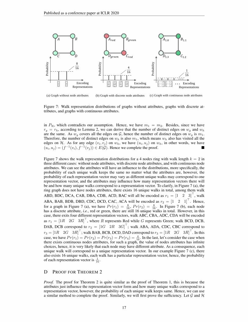
Figure 7: Walk representation distributions of graphs without attributes, graphs with discrete at-tributes, and graphs with continuous attributes.

in PH, which contradicts our assumption. Hence, we have m1 = m2. Besides, since we haverg = rh, according to Lemma 2, we can derive that the number of distinct edges on wg and whare the same. As wg covers all the edges on G, hence the number of distinct edges on wg is m1.Therefore, the number of distinct edges on wh is also m1, which means wh also has visited all theedges on H. As for any edge (vi, vj) on wh, we have (ui, uj) on wh, in other words, we have(ui, uj) = (f−1(vi), f

−1(vj)) ∈ E(G). Hence we complete the proof. �

Figure 7 shows the walk representation distributions for a 4 nodes ring with walk length k = 2 inthree different cases: without node attributes, with discrete node attributes, and with continuous nodeattributes. We can see the attributes will have an influence to the distributions, more specifically, theprobability of each unique walk keeps the same no matter what the attributes are, however, theprobability of each representation vector may vary as different unique walks may correspond to onerepresentation vector, and the attributes may influence how many representation vectors there willbe and how many unique walks correspond to a representation vector. To clarify, in Figure 7 (a), thering graph does not have nodes attributes, there exists 16 unique walks in total, among them walkABD, BDC, DCA, CAB, DBA, CDB, ACD, BAC will all be encoded as r1 = [1 2 3]

>, walkABA, BAB, BDB, DBD, CDC, DCD, CAC, ACA will be encoded as r2 = [1 2 1]

>. Hence,for a graph in Figure 7 (a), we have Pr(r1) = 8

16 , Pr(r2) = 816 . In Figure 7 (b), each node

has a discrete attribute, i.e., red or green, there are still 16 unique walks in total. However, in thiscase, there exits four different representation vectors, walk ABC, CBA, ADC, CDA will be encodedas r1 = [1R 2G 3R]

>, where R represents Red while G represents Green; walk BCD, DCB,DAB, DCB correspond to r2 = [1G 2R 3G]

>; walk ABA, ADA, CDC, CBC correspond tor3 = [1R 2G 3R]

>; walk BAB, BCB, DCD, DAD correspond to r3 = [1R 2G 3R]>. In this

case, we have Pr(r1) = Pr(r2) = Pr(r3) = Pr(r4) =416 . In the last, let’s consider the case when

there exists continuous nodes attributes, for such a graph, the value of nodes attributes has infinitechoices, hence, it is very likely that each node may have different attribute. As a consequence, eachunique walk will correspond to a unique representation vector. In our example Figure 7 (c), therealso exists 16 unique walks, each walk has a particular representation vector, hence, the probabilityof each representation vector is 1

16 .

D PROOF FOR THEOREM 2

Proof. The proof for Theorem 2 is quite similar as the proof of Theorem 1, this is because theattributes just influence the representation vector form and how many unique walks correspond to arepresentation vector, however, the probability of each unique walk keeps same. Hence, we can usea similar method to complete the proof. Similarly, we will first prove the sufficiency. Let G and H

17


be two isomorphic graphs with attributes, we will prove that the walk representations distribution ofG and H are the same. Suppose that A and B are the sets of possible walks of length k on G and Hrespectively. By applying the same analysis method as in the proof of Theorem 1, we can show thatthere exists a bijective mapping g : A→ B such that for ∀wi = v1v2v3 . . . vt ∈ A, we have

g(wi) = f(v1)f(v2) . . . f(vt) ∈ B, (12)

where f : V (G)→ V (H) satisfies ∀(vi, vj) ∈ E(G), we have (f(vi), f(vj)) ∈ E(H) and for ∀vi ∈V (G), the attribute of vi and f(vi) are the same. Hence, according to our encoding rule, wi andf(wi) will be encoded as the same representation vector, which means for each point (rgi , P r(rgi))in the representation distribution of G, we can find a point (rhi

, P r(rhi)) in the distribution of

H such that rgi = rhi, Pr(rgi) = Pr(rhi

). Thus, we can obtain the Wasserstein distance ofdistribution PG and the distribution PH is W1(PG , PH) = 0 via a similar approach as in Theorem1. In other words, we have PG = PH. In addition, the necessity proof of Theorem 2 is the same asTheorem 1. �

E GRAPHS WITH NODE ATTRIBUTES AND EDGE ATTRIBUTES

If both the nodes and edges in a graph have attributes, the graph is an attributed graph denoted byG = (V,E, α, β), where α : V → LN and β : E → LE are nodes and edges labeling functions,LN , LE are sets of labels for nodes and edges. In this case, the graph isomorphism are defined as:

Definition . Given two graphs G = (V (G), E(G), αG , βg) and H = (V (H), E(H), αH, βH), thenG and H are isomorphic with node attributes as well as edge attributes if there is a bijection f :V (G)⇔ V (H)

∀uv ∈ E(G)⇔ f(u)f(v) ∈ E(H), (13)αG(u) = αH(f(u)),∀u ∈ V (G), (14)

βG(u, v) = βH(f(u), f(v)). (15)

Corollary 1. Let G = (V (G), E(G)) and H = (V (H), E(H)) be two connected graphs with nodeattributes. Suppose we can enumerate all possible WEAVEs on G and H with a fixed-length k ≥2max{|E(G)|, |E(H)|}−1, where each WEAVE has a unique vector representation generated froma well-trained autoencoder. The Wasserstein distance between G’s and H’s WEAVE distributions is0 if and only if G andH are isomorphic with both node attributes and edge attributes.

Proof. When both nodes and edges of a graph are given attributes, the representation vectors of ran-dom walks will be different. However, just like the cases with only nodes attributes, the probabilityof each unique walk on the graph keeps same. Hence, we can follow a similar analysis method asTheorem 2 to complete this proof. �

DatasetIdentity Kernel DeepSet-MMD

Classification Clustering Classification ClusteringACC ACC NMI ACC ACC NMI

NCI1 0.6105 0.5510 0.0073 0.6382 0.5630 0.0095PROTEINS 0.7207 0.5957 0.0518 0.7103 0.5965 0.0438COLLAB 0.6720 0.5973 0.2108 0.6572 0.5668 0.2015

IMDB-BINARY 0.7660 0.5776 0.0241 0.7210 0.5219 0.0225IMDB-MULTI 0.4466 0.3816 0.0214 0.4258 0.3647 0.0168

Table 5: Representation evaluation based on classification and clustering down-stream tasks

F DEEPSET IN THE COMPONENT OF EMBEDDING DISTRIBUTIONS

In this section, we investigate whether DeepSet (Zaheer et al., 2017) is an effective technique fordistribution embedding. In particular, we employ DeepSet to replace the multi-layer neural net-work for feature mapping function approximation, and similarity values generated by MMD serve

18


as supervision signals to guide DeepSet training. In our experiments, we compare the SEED imple-mentation based on DeepSet with MMD (DeepSet in Table 5) with the SEED implementation basedon the identity kernel (Identity Kernel in Table 5). We also observe that the MMD does not havesignificant performance difference. The result confirms that DeepSet could be a strong candidate forthe component of Embedding subgraph distributions.

G ABLATION STUDY ON WEAVE

Feature utilized Classification ACC Clustering ACC Clustering NMI

Only node feature 0.6444 0.6744 0.0625Only earliest visit time 0.8112 0.8014 0.3214Node feature + Earliest visit time 0.8222 0.7260 0.1567

Table 6: The impact of node feature and earliest visit time in WEAVE based on MUTAG dataset

In this section, we investigate the impact of node features and earliest visit time in WEAVE. InTable 6, Only node feature means only node features in WEAVE are utilized for subgraph encoding(which is equivalent to vanilla random walks), only earliest visit time means only earliest visit timeinformation in WEAVE is used for subgraph encoding, and Node feature + earliest visit time meansboth information is employed. We evaluate the impact on the MUTAG dataset. As shown above,it is crucial to use both node feature and earliest visit time information in order to achieve the bestperformance. Interestingly, on the MUTAG dataset, we observe that clustering could be easier ifwe only consider earliest visit time information. On the MUTAG dataset, node features seem tobe noisy for the clustering task. As the clustering task is unsupervised, noisy node features couldnegatively impact its performance when both node features and earliest visit time information areconsidered.

H NYSTROM APPROXIMATION IN THE SEED FRAMEWORK

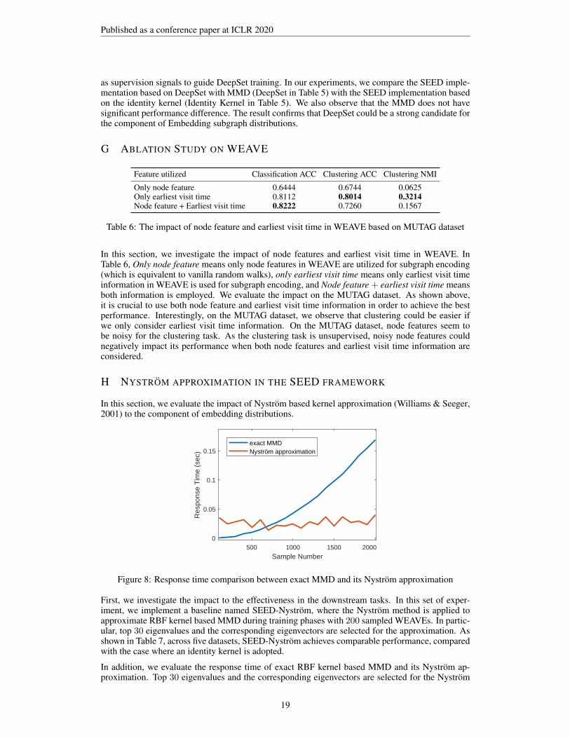
In this section, we evaluate the impact of Nystrom based kernel approximation (Williams & Seeger,2001) to the component of embedding distributions.

500 1000 1500 2000

Sample Number

0

0.05

0.1

0.15

Res

pons

e T

ime

(sec

)

exact MMDNyström approximation

Figure 8: Response time comparison between exact MMD and its Nystrom approximation

First, we investigate the impact to the effectiveness in the downstream tasks. In this set of exper-iment, we implement a baseline named SEED-Nystrom, where the Nystrom method is applied toapproximate RBF kernel based MMD during training phases with 200 sampled WEAVEs. In partic-ular, top 30 eigenvalues and the corresponding eigenvectors are selected for the approximation. Asshown in Table 7, across five datasets, SEED-Nystrom achieves comparable performance, comparedwith the case where an identity kernel is adopted.

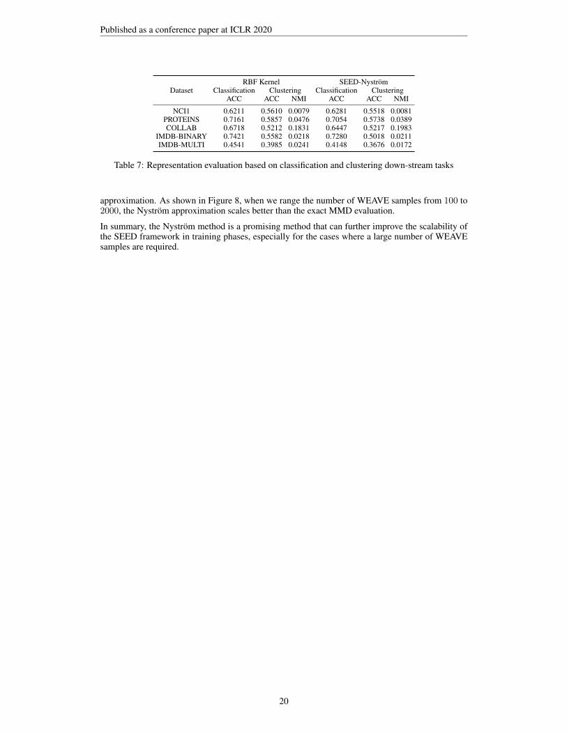
In addition, we evaluate the response time of exact RBF kernel based MMD and its Nystrom ap-proximation. Top 30 eigenvalues and the corresponding eigenvectors are selected for the Nystrom

19


DatasetRBF Kernel SEED-Nystrom

Classification Clustering Classification ClusteringACC ACC NMI ACC ACC NMI

NCI1 0.6211 0.5610 0.0079 0.6281 0.5518 0.0081PROTEINS 0.7161 0.5857 0.0476 0.7054 0.5738 0.0389COLLAB 0.6718 0.5212 0.1831 0.6447 0.5217 0.1983

IMDB-BINARY 0.7421 0.5582 0.0218 0.7280 0.5018 0.0211IMDB-MULTI 0.4541 0.3985 0.0241 0.4148 0.3676 0.0172

Table 7: Representation evaluation based on classification and clustering down-stream tasks

approximation. As shown in Figure 8, when we range the number of WEAVE samples from 100 to2000, the Nystrom approximation scales better than the exact MMD evaluation.

In summary, the Nystrom method is a promising method that can further improve the scalability ofthe SEED framework in training phases, especially for the cases where a large number of WEAVEsamples are required.

20

Documents

INDUCTIVE AND UNSUPERVISED REPRESENTATION …