IIIInnnnvvvveeeessssttttiiiiggggaaaattttiiiinnnngggg aaaannnn aaaassssssssoooocccciiiiaaaattttiiiioooonnnn bbbbeeeettttwwwweeeeeeeennnn

sunspot numbers and summersunspot numbers and summersunspot numbers and summersunspot numbers and summer

rainfall in Indiarainfall in Indiarainfall in Indiarainfall in India

September 15

IIIInnnnvvvveeeessssttttiiiiggggaaaattttiiiinnnngggg aaaannnn aaaassssssssoooocccciiiiaaaattttiiiioooonnnn bbbbeeeettttwwwweeeeeeeennnn

sunspot numbers and summersunspot numbers and summersunspot numbers and summersunspot numbers and summer----mmmmoooonnnnssssoooooooonnnn

3rd International Conference on

Hydrology & Meteorology

September 15-16, 2014, HICC, Hyderabad, India

ISMR-an overviewhe summer monsoon during the months of June to Sdia. Hence, the prediction of Indian summer monso

high variability has significant impact on economy of the country.

During ISM the Western Ghats and the northeast region receives precipitation due to terplay and eastern India i.e. Orissa, Chhattisgarh a

monsoon trough.

ost of the statistical forecasting techniques available

10/13/2014 Hydrology 2014

ost of the statistical forecasting techniques availabledeterministic prediction without any measure of its inherent uncertainty.

s probabilistic predictions have the ability to quantimakers than deterministic forecasts

Recently some studies have raised the issues of making probabilistic forecast using GCMs.

an overviewo September (JJAS) is the major rainfall season for nsoon rainfall (ISMR) is always in high demand as it

high variability has significant impact on economy of the country.

During ISM the Western Ghats and the northeast region receives precipitation due to orographich and West Bengal receives precipitation due to

ble till dates have concentrated only in generating a

Hydrology 2014

ble till dates have concentrated only in generating adeterministic prediction without any measure of its inherent uncertainty.

ntify the uncertainty, it has more potential to decisio

Recently some studies have raised the issues of making probabilistic forecast using GCMs.

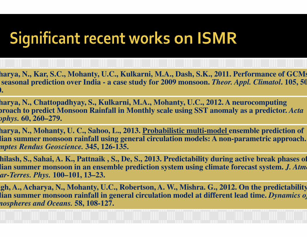
Acharya, N., Kar, S.C., Mohanty, U.C., Kulkarni, Mfor seasonal prediction over India - a case study for 2009 monsoon. 520.

Acharya, N., Chattopadhyay, S., Kulkarni, M.A., Mohantyapproach to predict Monsoon Rainfall in Monthly scale using SST anomaly as a predictor. Geophys. 60, 260–279.Geophys. 60, 260–279.

Acharya, N., Mohanty, U. C., Sahoo, L., 2013. Probabilistic multiIndian summer monsoon rainfall using general circulation models: A nonComptes Rendus Geoscience. 345, 126-135.

Abhilash, S., Sahai, A. K., Pattnaik , S., De, S., 201Indian summer monsoon in an ensemble prediction system using climate forecast system. Solar-Terres. Phys. 100–101, 13–23.

Singh, A., Acharya, N., Mohanty, U.C., Robertson, A. W., Indian summer monsoon rainfall in general circulation model at different lead time. Atmospheres and Oceans. 58, 108-127.

, M.A., Dash, S.K., 2011. Performance of GCMsa case study for 2009 monsoon. Theor. Appl. Climatol. 105, 505

Mohanty, U.C., 2012. A neurocomputingapproach to predict Monsoon Rainfall in Monthly scale using SST anomaly as a predictor. Acta

Probabilistic multi-model ensemble prediction of Indian summer monsoon rainfall using general circulation models: A non-parametric approach.

013. Predictability during active break phases of Indian summer monsoon in an ensemble prediction system using climate forecast system. J. Atmo

, U.C., Robertson, A. W., Mishra. G., 2012. On the predictability Indian summer monsoon rainfall in general circulation model at different lead time. Dynamics of

The Effects of Solar Variability on the Earth's Climate

Author(s): Joanna D. Haigh

“The extent to which changes in solar activity affect climate has been tover many years and has often been the cause of speculation and controversy

As observational and improve, and our understanding of the natural internal variability of the cmore feasible both to detect solar signals in climate Haigh

Source: Philosophical Transactions: Mathematical, Physical and Engineering Sciences, Vol. 361, No. 1802, (Jan. 15, 2003), pp. 95-111

more feasible both to detect solar signals in climate records and to investigate the mechanisms whereby the solar influence acts.

This subject is an interesting and complex scientific area to spractical importanceand anthropogenireliable estimates can be made of the potential future impacts of human activities on climate

10/13/2014 Hydrology 2014

The extent to which changes in solar activity affect n the subject of considerable investigation

over many years and has often been the cause of speculation and controversy.

As observational and modelling techniques improve, and our understanding of the natural internal

e climate system advances, it is becoming more feasible both to detect solar signals in climate more feasible both to detect solar signals in climate records and to investigate the mechanisms whereby the solar influence acts.

This subject is an interesting and complex o study, but it is now also of considerable

practical importance in terms of differentiating natural enic causes of climate change so that more

reliable estimates can be made of the potential future impacts of human activities on climate.”

A brief overview of SunspotA brief overview of Sunspot

10/13/2014 Hydrology 2014

A brief overview of SunspotA brief overview of Sunspot

Although the details of sunresearch, it appears that sumagnetic flux tubes in theup" by differential rotation.

If the stress on the tubes rerubber band and punctureat the puncture points; the

10/13/2014 Hydrology 2014

at the puncture points; thedecreases; and with it surface temperature.

Due to its link to other kindcan be used to help predict space weather, the state of the ionosphere, and hence the conditions of shortpropagation or satellite cosunspot cycle) are frequenwarming.

f sunspot generation are still a matter of at sunspots are the visible counterparts of the Sun's convective zone that get "wound

up" by differential rotation.

es reaches a certain limit, they curl up like ure the Sun's surface. Convection is inhibit

; the energy flux from the Sun's interior ; the energy flux from the Sun's interior decreases; and with it surface temperature.

kinds of solar activity, sunspot occurrencecan be used to help predict space weather, the state of the ionosphere, and hence the conditions of short-wave radio

e communications. Solar activity (and the uently discussed in the context of global

10/13/2014 Hydrology 2014

Bhattacharyya, S., and R.

associa

activity”,

doi:10.1029/2004GL021044.

10/13/2014 Hydrology 2014

It is found that the average rainfall is higher iseven rainfall indices during periods of greater

activity, at confidence levels varying from 75%99%, being 95% or greater in three of them. U

wavelet techniques it is also found that the powthe 8–16 y band during the period of higher s

activity is higher in 6 of the 7 rainfall time serieconfidence levels exceeding 99.99%.

These results support existenceconnections between Indian rain

Bhattacharyya, S., and R. Narasimha (2005), “Possibl

ciation between Indian monsoon rainfall and sola

activity”, Geophys. Res. Lett., 32, L05813,

doi:10.1029/2004GL021044.

These results support existenceconnections between Indian rain

and solar activity

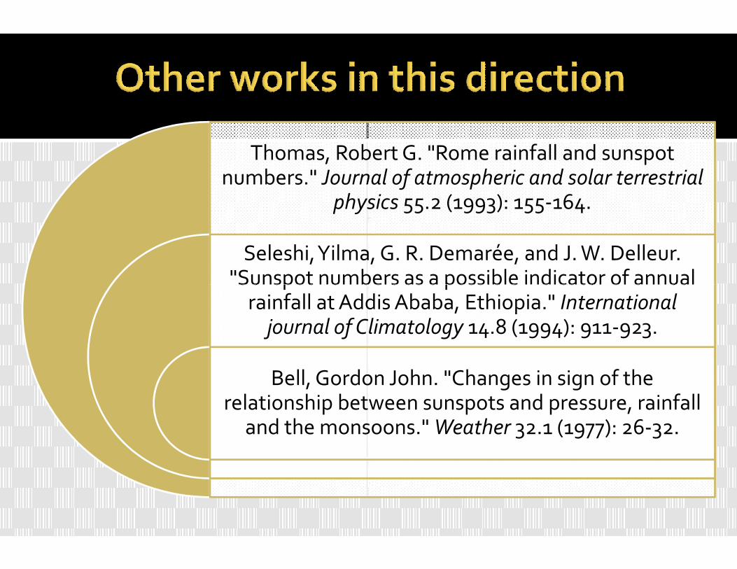
Thomas, Robert G. "Rome rainfall and sunspot numbers." Journal of atmospheric and solar terrestrial

physics

Seleshi, Yilma"Sunspot numbers as a possible indicator of annual "Sunspot numbers as a possible indicator of annual

rainfall at Addis Ababa, Ethiopia." journal of Climatology

Bell, Gordon John. "Changes in sign of the relationship between sunspots and pressure, rainfall

and the monsoons."

Thomas, Robert G. "Rome rainfall and sunspot Journal of atmospheric and solar terrestrial

physics 55.2 (1993): 155-164.

Yilma, G. R. Demarée, and J. W. Delleur. "Sunspot numbers as a possible indicator of annual "Sunspot numbers as a possible indicator of annual

rainfall at Addis Ababa, Ethiopia." International journal of Climatology 14.8 (1994): 911-923.

Bell, Gordon John. "Changes in sign of the relationship between sunspots and pressure, rainfall

and the monsoons." Weather 32.1 (1977): 26-32.

In the present work we shall investigate whether there is any association between the S(June–September; abbreviated as JJASIndia.

We shall analyze the autocunder consideration and safter Box–Cox transformation of both of the time series.

We shall also examine thethe summer monsoon rainfall over India.

10/13/2014 Hydrology 2014

In the present work we shall investigate whether there is any e SN time series and the summer monsoon

September; abbreviated as JJAS) rainfall time series over

tocorrelation structure of the time series d subsequently execute a spectral analysis

Cox transformation of both of the time series.

the possibility of using SN as a predictor forthe summer monsoon rainfall over India.

We consider the summer monsoon (JJAS) rainfall time series over

India

collected from the website of the

10/13/2014 Hydrology 2014

collected from the website of the Indian Institute of Tropical

Meteorology, Pune, and the mean annual SN time series

collected by the National Oceanic and Atmospheric Administration

(NOAA), Boulder, Colorado during the period from 1935 to 1998.

No persistence

we find a clea

year cycle in

ACF

Skewness (Pearson) for ISMR=0.049 , for SN=0.477

It is found that both of the time series under consideration are positively skewed.

Thus, we apply a Box–Cox transformation to the time series to stabilize the variance as follows

where Xt is the original series, G is the sample geometric mean, λ is the transformation parameter, and Zt is the transformed series.

10/13/2014 Hydrology 2014

1

1−

−=

λ

λ

λG

XZ t

t

For the rainfall time series, λ = 0.716 and G =203.81

and for the SN time series λ = 0.366, and G =52.839

After transforming the time series by Box–Cox, we carry out a spectral analysis of the time series. Detailed theory of the spectral analysis is available in Wilks (2006, pp. 83–86).Any data series consisting of n points can be represented by adding together a series of represented by adding together a series of n/2 harmonic functions as:

Ak and Bk are Fourier coefficients, yt is the entry to the time series at time t. Spectral density is

10/13/2014 Hydrology 2014

22

kkk BAC +=

The advantage of this new perspective is thatit allows us to see separately the contributions to a time series that are made by processes varying at different speeds, thatis by processes operating at a spectrum of different frequenciesdifferent frequencies

The horizontal axis of a spectrum can also bescaled according to the reciprocal of the frequency, or the period of the kth harmonicas:

τk=n/k, where k=1, 2, ..., n/2=32.

Most important variations in the data series are represented byharmonics τ4 =64/4=16 and τ 31 =64/31=2.06, τ 32 =2.

Rainfall

10/13/2014 Hydrology 2014

Most important variations in the data series are represented bthe harmonics τ6 = 64/6 = 10.67. Other important harmonics aτ 5 and τ 7.

Sunspot

We revealed that τ5 is a prseries. Thus, we can consider

From this, we attempt to establish a predictorFrom this, we attempt to establish a predictorrelationship between SN and monsoon rainfall.

As the common harmonicspectra, it is not logical to go for a linear regression.

Furthermore, the correlationindicates the absence of any series.

10/13/2014 Hydrology 2014

a prominent harmonic in both of the time we can consider τ5 as a common harmonic.

From this, we attempt to establish a predictor–predictandFrom this, we attempt to establish a predictor–predictandrelationship between SN and monsoon rainfall.

onic contributes very little to the entire spectra, it is not logical to go for a linear regression.

tion between the two time series is 0.037, whichany linear association between the two time

Cross Correlation

present the cross-correlation between SNs

rainfall amounts.observed that the

correlation

Hydrology 2014

Cross-correlation is

a function of a time

correlationamounts always lie in

range [−0.2,0.2].further indicates

absence of any linearassociation between the

time series underconsideration.

xyρ

n is a measure of similarity of two waveforms as

a function of a time-lag applied to one of them.

( )( )[ ] ( )YXYmnXn YXE σσµµ /−−= +

As τ5 has been revealed as common to both of the time

series, we can try to determine some relationships within a period of 64/5=12.8 years.

Taking all these into account, we decided to test a model

based on 5-year averages of the observations.

10/13/2014 Hydrology 2014

In cross-correlation between SN and rainfall, we find that there are significant positive and negative spikes at lags

separated by approximately 5.

This means that, in five time steps, the correlation is

changing from extremely negative to extremely positive.

Hydrology 2014

Moving Average

We find that moving the average to 5 years gives more smoothness to the time series. Thus, we try to estimate the 5-year average monsoon rainfall amount over India using the corresponding 5-India using the corresponding 5-year average SNs as predictor.

We present the actual time series and those after taking the 5-year average. It can be seen that the time series are becoming smoother after taking the 5-year averages.

ANN model generation

� 1. A priori knowledge of the underlying process is not required.

� 2. Existing cvarious aspects of the process under

We consider a time series

pertaining to the study period

1998. Thus, we have 64

data in each time series. We

denote this series by x1, x2, x3,

, x64.

(see: SILVERMAN, D. a

precipitation prediction in California.

various aspects of the process under investigation need not be recognized.

� 3. Solution cby standardare not preset.

� 4. Constrainare neither assumed nor enforced

, x64.

From the original time series,

we derive a new time series

whose entries are

10/13/2014 Hydrology 2014

5

...

5

...

,5

...

64616060

632

521

yyy

xxx

xxx

+++=

+++

+++

1. A priori knowledge of the underlying process is not required.

ng complex relationships among thevarious aspects of the process under

Advantages of ANN D. and DRACUP, J.A., 2000, Artificial neural networks and long-

precipitation prediction in California. Journal of Applied Meteorology, 39, pp. 57–66.

various aspects of the process under investigation need not be recognized.

ion conditions, such as those requireard optimization or statistical mode

are not preset.raints and a priori solution structure

are neither assumed nor enforced.

Outline of an ANN

Details of the theory of ANNs are available in Bishop (1995), Rojas (1996) and in many other books.Geophysical systems are generally characterized by various degrees of chaos and non-linearity .

Outline of a Multilayer

(MLP)

Numerous examples are available where the ANN has been implemented in forecasting atmospheric phenomena. Some significant examples include Gardner and Dorling (1998), Hsieh and Tang (1998).

Gardner MW, Dorling SR. 1998. Multilayer Perceptron- a review of applications in atmospheric sciences. Atmospheric Environment

2627–2636.

Hsieh,W.W. and Tang, B., 1998, Applying neural network models to prediction and data analysis in meteorology and oceanography. Bulletin of the American Meteorological Society, 79, pp. 1855–1870.

10/13/2014 Hydrology 2014

( )e

xf+

=1

1

Outline of a Multilayer Perceptron

MLP learning

This equation reprweight vector b

the advent of the

backpropagation algorithm a vast

of improvements has been

the technique for supervised

of MLP. The backpropagation

algorithm looks for minimum error

in weight space using the

of gradient descent.

Rojas R. 1996. Neural Networks: A Systematic Introduction. Springer

Verlag New York, Inc.: New York.

Medsker LR, Jain LC. 2000.

Applications. CRC Press: Boca Raton, FL.

weight vector badaptation is pea set of pairs of input and target vectors.

of gradient descent.

10/13/2014 Hydrology 2014

kk dw η+=

( )kwE−∇=

) ( )1−∆+∂

∂−= lw

w

Ek

k

αγ

The positive constant

the negative gradient of the output error function

the i-th correction for weight w

γ and α are the le

denotes the error

represents an iteration process that finds the optimor by adapting the initial weight vector w0. This

Neural Networks: A Systematic Introduction. Springer-

New York, Inc.: New York.

LR, Jain LC. 2000. Recurrent Neural Networks: Design and

Applications. CRC Press: Boca Raton, FL.

or by adapting the initial weight vector w0. This is performed by presenting to the network sequen

a set of pairs of input and target vectors.

The positive constant η is called the learning rate. The direction vector d

gradient of the output error function E.

correction for weight wk

he learning and momentum rate respectively, and E

denotes the error.

The input matrix for the generation of the ANN

(60 × 2), where the first column pertains to the

pertains to the predictand

From the data series,

70% of the data are

chosen as the training

set and the remaining

30% of the data are

chosen as the test set.

An adaptive gradient

learning in the

cascade mode is used

with a maximum

allowable hidden layer

size of 60.

The sigmoid function

(f (x) = (1 + e

taken as the activation

function.

10/13/2014 Hydrology 2014

The input matrix for the generation of the ANN-based prediction model is of the order of

the predictor (i.e. the SN) and the second column

(i.e. the monsoon rainfall).

After training and

The sigmoid function

(f (x) = (1 + e−x)−1) is

taken as the activation

function.

Minimization of the

mean squared error is

chosen as the

stopping criterion.

After training and

testing the networ

and validating ove

the entire set of 60

data, the optimum

network architectur

is available with sev

hidden nodes.

Hydrology 2014

Willmott’s Index

We find that d =0.795 in the present model. This indicates, in general, a good model.The model outputs are

presented here, where all the validation cases are the validation cases are presented.In this figure, it is found

that in various validation cases, the actual and predicted values have almost coincided. In many cases, although

they are not coincident, a close association is visible.

Confusion matrix

A confusion matrix was generated to view the prediction capacity of the ANN model.

A confusion matrix is a square matrix whose rows and columns represent the subranges for the real-world target and model outputs, respectively.

The value in the (i,j) position of the matrix is the number of records for which the real-world target output is

ith subrange and whose real-world model output is within the jthsubrange.

10/13/2014 Hydrology 2014

This table shows that for the

observations and 16 p

subrange. For the subrange

10 predictions, which means that there is 71% accuracy for this

Thus, it can be interpr

possibility of an accur

amounts.

This table shows that for the subrange 25.61–51.98 mm there are 20

16 predictions. Thus, there is 80% accuracy for this

subrange 51.975–78.34 mm, there are 14 observations

10 predictions, which means that there is 71% accuracy for this subrange

erpreted that for lower rainfall amounts there is more

ccurate forecast by ANN than in the case of higher rainf

We analysed the autocorrelation structures, which showed a wave pattern in the case of SN. However, in the case of the monsoon rainfall, no such pattern was discerned.

Considering previous studies on the association between solar activities and climate, we tried to find some association despite the apparent non-linearity implied by the very low cross-correlation.

Implementing spectral analysis we obtained a common prominent harmonic between the two time series under consideration. The common harmonic was the fifth harmonic, which implies a common common harmonic was the fifth harmonic, which implies a common cycle of 12.8 years.

We decided to implement an ANN in the form of multilayer perceptrons with sigmoid non-linearity.

We derived new time series by averaging the observations for 5 years. Finally, it was revealed that by the implementation of the ANN, an average of 5-year SNs can give some estimate for the 5summer monsoon rainfall over India.

10/13/2014 Hydrology 2014

Concluding

remarksthe autocorrelation structures, which showed a wave

pattern in the case of SN. However, in the case of the monsoon rainfall,

Considering previous studies on the association between solar activities and climate, we tried to find some association despite the apparent

correlation.

Implementing spectral analysis we obtained a common prominent harmonic between the two time series under consideration. The common harmonic was the fifth harmonic, which implies a common common harmonic was the fifth harmonic, which implies a common

We decided to implement an ANN in the form of multilayer linearity.

We derived new time series by averaging the observations for 5 years. Finally, it was revealed that by the implementation of the ANN, an

year SNs can give some estimate for the 5-year averaged summer monsoon rainfall over India.

Hydrology 2014

Thank YouThank YouThank YouThank You