Instructions for use

Title Effects of acorn abundance on density dependence in a Japanese wood mouse (Apodemus speciosus) population

Author(s) Saitoh, Takashi; Vik, Jon Olav; Stenseth, Nils Chr.; Takanishi, Toshikazu; Hayakashi, Shintaro; Ishida, Nobuo;Ohmori, Masaaki; Morita, Toshio; Uemura, Shigeru; Kadomatsu, Masahiko; Osawa, Jun; Maekawa, Koji

Citation Population Ecology, 50(2): 159-167

Issue Date 2008-04

Doc URL http://hdl.handle.net/2115/33873

Rights The original publication is available at www.springerlink.com

Type article (author version)

File Information Saitoh_et_al_2008.pdf

Hokkaido University Collection of Scholarly and Academic Papers : HUSCAP

- 1 -

Effects of acorn abundance on density dependence in a Japanese wood

mouse (Apodemus speciosus) population2

Takashi Saitoh · Jon Olav Vik · Nils Chr. Stenseth · Toshikazu Takanishi · Shintaro Hayakashi4

· Nobuo Ishida · Masaaki Ohmori · Toshio Morita · Shigeru Uemura · Masahiko Kadomatsu ·

Jun Osawa · Koji Maekawa6

T. Saitoh · K. Maekawa8

Field Science Center, Hokkaido University, North 11, West 10, Sapporo 060-0811, Japan

10

J. O. Vik · N. C. Stenseth

Centre for Ecological and Evolutionary Synthesis (C.E.E.S.), Department of Biology,12

University of Oslo, P.O. Box 1066 Blindern, N-0316 Oslo, Norway

14

T. Takanishi · S. Hayakashi · N. Ishida · M. Ohmori

Uryu Experimental Forest, Field Science Center, Hokkaido University, Moshiri, Horokanai16

074-0741, Japan

18

S. Uemura

Northern Forestry Research and Development Office, Field Science Center, Hokkaido20

University, Tokuda 250, Nayoro 096-0071, Japan

22

M. Kadomatsu

Nakagawa Experimental Forest, Field Science Center, Hokkaido University, Otoineppu 098-24

2501, Japan

26

J. Osawa

Graduate School of Agriculture, Hokkaido University, North 9, West 9, Sapporo 060-0811,28

Japan

30

Corresponding author: Takashi Saitoh

- 2 -

Field Science Center, Hokkaido University32

North 11, West 10, Sapporo 060-0811, Japan

Tel: +81-11-706-2590; E-mail: tsaitoh@fsc.hokudai.ac.jp34

Running head: Density dependence in wood mouse36

The revised version consists of38

26 pages of text,

1 table,40

1 page of figure legends,

3 figures, and42

2 pages for Electronic Supplementary Material.

- 3 -

Abstract We analysed the effects of Quercus crispula acorn abundance on the density44

dependence of the large Japanese wood mouse Apodemus speciosus using time series data

(1992–2007). The data were obtained in a forest in northern Hokkaido, Japan, by live-46

trapping rodents and directly counting acorns on the ground. Acorn abundance in one year

clearly influenced the abundance of wood mice in the following year in all models examined48

based on the Gompertz and Ricker model; in addition, the abundance of wood mice had

effects on the population. Acorn abundance influenced the strength of density dependence50

(intraspecific competition) of the wood mouse population. When the abundance of acorns was

high, density dependence was relaxed and as a result the equilibrium density at which the52

population growth rate decreased to zero became higher. Those effects of acorn abundance

were regarded as a nonlinear perturbation effect (sensu Royama 1992). The nonlinearity of54

density dependence was also detected; higher densities had stronger effects on population

growth rates.56

Keywords Dynamics · Intraspecific competition · Lateral perturbation effect · Masting ·58

Nonlinear density dependence · Nonlinear perturbation effect

60

- 4 -

Introduction

Rodent population dynamics are a synergetic phenomenon, including effects of intraspecific62

competition, trophic interactions, weather, and disease (Batzli 1992), as well as other animal

species (Royama 1992; Turchin 2003). Despite their complexity, some consensus has been64

reached among population ecologists regarding population cycles (periodic large-scale

fluctuations with high amplitude) which have been reported for vole and lemming populations66

of northern Eurasia and North America. Trophic interactions may generate population cycles

through delayed density dependence (Stenseth 1999; Klemola et al. 2003; Korpimäki et al.68

2004), which may be due to interactions with food supply or natural enemies such as

predators, parasites, and diseases. However, in populations that exhibit irregular outbreaks,70

density-independent factors may have more profound effects than in cyclic populations, and

direct, rather than delayed, density dependence is predominant (Royama 1992; Saitoh et al.72

1999; Lima et al. 2006).

74

Wood mice (genus Apodemus) appear to have dynamics dominated by irregular outbreaks

related to years of abundant seed production (Flowerdew 1985; see also Montgomery 1989a,76

b). Masting of seeds (synchronous intermittent production of large seed crops) improves

reproduction and survival of Apodemus (Montgomery et al. 1991: see Wilson et al. 1993 and78

Shimada and Saitoh 2006 for reviews) and often causes a high density of Apodemus

populations (Jensen 1982; Miguchi 1988; Mallorie and Flowerdew 1994). Therefore,80

populations of Apodemus are likely to be influenced by seed production, in addition to direct

density dependence (Saitoh et al. 1999).82

- 5 -

Intraspecific competition for food or space is generally considered a mechanism of direct84

density dependence (Stenseth et al. 1996; Saitoh et al. 1997, 1999; Prévot-Julliard et al. 1999;

Lima et al. 2001, 2002a, 2002b; Murúa et al. 2003), although generalist predators are86

considered a main agent for direct density dependence in Fennoscandia (Hansson and

Henttonen 1988; Hanski et al. 2001; Turchin and Hanski 2001; Korpimäki et al. 2004). If88

intraspecific competition is a principle cause of direct density dependence, then density

dependence could be influenced by the abundance of resources.90

Royama (1992) suggests that resources which can be measured by a simple per-capita share92

of the resource (e.g., nests holes for birds) have linear effects on density dependence (“lateral

perturbation effect”), while resources that are gradually depleted (e.g., crops for birds) have94

nonlinear effects on density dependence (“nonlinear perturbation effect”). A “lateral

perturbation effect” shifts the equilibrium density at which population growth rate takes zero,96

but does not influence the strength of density dependence. In contrast, a “nonlinear

perturbation effect”, by altering the strength of density dependence, influences the equilibrium98

density. Yoccoz et al. (2001) examined the density-dependent structure of bank vole

(Clethrionomys glareolus) populations, assuming that density dependence would be relaxed100

under conditions of abundant food resources; however, the effects of food addition on density-

dependent structure were negligible. Food habits of the bank vole are intermediate between102

herbivorous and granivorous, and they consume a large variety of food items (Hanson 1985).

Since they do not depend on a specific food resource, the interactions between food and104

rodents may be complex. Thus, the relationship is expected to be clearer in other rodent

species that rely on a specific food resource.106

- 6 -

The relationship between masting of the oak (Quercus crispula Blume) and population108

dynamics of the large Japanese wood mouse (Apodemus speciosus (Temmink, 1844)) is a

suitable system with which to answer the question about the interaction between food and110

rodents. Acorns of Q. crispula are nutritionally rich (Shimada 2001), and A. speciosus, which

is a small (40–60 g) mouse endemic to Japan, caches acorns (Miyaki and Kikuzawa 1988;112

Soné and Kohno 1996). The Field Science Centre of Hokkaido University has monitored the

abundance of rodents and acorns from 1992 to the present, and Saitoh et al. (2007) have114

detected clear effects of acorn abundance on the population dynamics of A. speciosus.

116

Here, we analysed effects of acorn abundance on density dependence of a wood mouse

population using time series data spanning the period from 1992 to 2007. We conclude that118

the strength of density dependence is altered by acorn abundance and that the nature of

density dependence is essentially related to the interaction with resources.120

Materials and methods122

Study area

The study was conducted in the Uryu Experimental Forest (44°03’–29' N, 142°1’–20' E) of124

Hokkaido University in Horokanai, Hokkaido, Japan, located in the cool temperate wet

climate zone. The yearly average temperature is 4.2°C (3.4 - 4.8°C between 1994 and 2006),126

annual precipitation is 1224.1 mm raging from 961.5 to 1540.5 mm in the same period, and

the maximum depth of accumulated snow exceeds 200 cm every year.128

- 7 -

Rodent abundance was investigated in two plots (see the map in Saitoh et al. 2007): one (A)130

was located in a forest plantation and the other (B) in a typical natural forest. The plantation

was a 6.78-ha forest, where 4800 seedlings of Japanese ash (Fraxinus mandshurica var.132

japonica), 900 seedlings of Ezo spruce (Picea glehnii), and 350 seedlings of todo fir (Abies

sachalinensis) were planted in 1985. Since that time, however, this forest has become a134

secondary forest with birch (Betula ermani) as a dominant species. The natural forest

consisted of broad-leaved trees and conifers. Dominant species were Acer mono, Q. crispula,136

Betula ermani, Sorbus commixta, Abies sachalinensis, and Picea glehnii. The undergrowth of

the natural forest was dominated by dwarf bamboo, Sasa senanensis and S. kurilensis. The138

distance between the two plots was 970 m.

140

Acorn abundance was investigated at two other study sites in natural forests located 6300 m

apart. The distance between the rodent plots and acorn count plots was approximately 5 km.142

Large Japanese wood mouse144

Although seven rodent species (Apodemus speciosus, A. argenteus, A. peninsulae,

Clethrionomys rufocanus, C. rutilus, Tamias sibiricus, and Rattus norvegicus) were recorded in146

the study plots, we focused on the large Japanese wood mouse A. speciosus because this

species is dominant in the study area, and a clear effect of acorn abundance on the mouse148

population has already been demonstrated (Saitoh et al. 2007).

150

Apodemus speciosus is a wood mouse that weighs 40–60 g and is endemic to Japan. The main

reproductive season is from April/May to September/October in Hokkaido (Fujimaki 1969;152

- 8 -

Murakami 1974; Kondo and Abe 1978). The main dietary items are seeds and invertebrates,

mainly insects. There are no reports that green plants dominate over other food items in their154

diets in Hokkaido. The diet of wood mice is thus predominantly granivorous and

subdominantly insectivorous. Caching behaviour is well developed (Miyaki and Kikuzawa156

1988; Soné and Kohno 1996). Among the sympatric species that we recorded, there is no

evidence of inter-generic competition (e.g., Abe 1986), although congeneric interactions are158

thought to occur (Ota 1968; Abe 1986). Apodemus speciosus is dominant over A. argenteus

(Sekijima and Soné 1994).160

Rodent abundance162

Rodent abundance was recorded in the two study plots from 1992 to 2007. Trapping was

carried out for 3 days each autumn (September or early October) at each plot using 50164

Sherman-type live traps baited with oats and placed at 10-m intervals in a grid pattern. All

rodents were identified by toe clipping upon first capture. Species, location, identity, sex,166

body weight (once or more per trapping session), and reproductive status were recorded upon

capture. The methods of animal handling conformed to the guidelines of the American168

Society of Mammalogists (Animal Care and Use Committee 1998).

170

Acorn count

Acorn abundance was recorded from 1991 to 2006 in the two study sites (see the map in172

Saitoh et al. 2007). In total, 15 and 17 oak trees (Q. crispula) were selected for investigation in

Forest 408 and Forest 422, respectively. All acorns found on the ground within a 10-m radius174

of a selected tree were counted. This direct count was carried out three or four times at 2- to

- 9 -

20-day intervals every autumn (September–November). The frequency and interval of the176

direct counts were adjusted to acorn abundance in a year; i.e., trees were more frequently

investigated at shorter intervals in a high-abundance year. Although the selected trees were178

investigated continuously during the study period, four trees in Forest 422 were excluded in

2004 because they were heavily damaged by a typhoon in 2004.180

In addition to the direct acorn counts, 50 seed traps with 0.5-m2 aperture were set at 10-m182

intervals in a grid pattern in the rodent plot B in the natural forest. The seed traps were

examined monthly from June to October between 1993 and 2005, and the number of collected184

seeds was counted for each tree species. Although data from the seed traps are preferable

because the investigation was performed in the rodent plot using standardised methods, the186

study period was shorter than that for the direct counts in Forest 408 and Forest 422. Because

the acorn abundance data from the two methods were highly correlated (Pearson’s correlation188

coefficient rs = 0.825), we used the data from Forest 408 and Forest 422 for the following

analyses because of the longer study period.190

Models192

Although small rodent populations generally exhibit a second-order autoregressive structure

on an annual basis (e.g., Bjørnstad et al. 1995; Stenseth 1999), in populations of the wood194

mouse A. speciosus, direct density dependence dominates over delayed density dependence,

and there is no evidence for the effect of delayed density dependence (Saitoh et al. 1999).196

Thus, we considered only direct density dependence in a model to predict mouse abundance.

The breeding season of the wood mouse is from spring to autumn. Because Q. crispula acorns198

- 10 -

become available to rodents from late September, acorn abundance has little influence on

mouse reproduction in the current year and may have a minor effect on mouse populations in200

the current year. Acorn effects on mouse populations may appear in the next year through the

following process: in a mast year, mice may gain weight in autumn and cache acorns for the202

winter, which results in higher overwintering survival; more mice reproduce during the next

spring, and the population increases. Thus, letting xt correspond to the log-transformed ‘true’204

abundance of mice in year t, ignoring higher-order terms, the mouse abundance in year t may

be expressed using the density dependence parameter α1 (the direct density dependence)206

together with effects of acorn abundance, α2:

xt = (1 + α1)xt-1 + α2At-1 + εt (Model 1),208

where At is the log-transformed ‘true’ abundance of acorns in year t, and the process

stochasticity, εt, is assumed to be normally distributed with mean zero and a constant variance210

(σ2). Since the term of α2At-1 influences the equilibrium density, not altering the strength of

density dependence, this effect is conceptualised as “lateral perturbation effect” by Royama212

(1992).

214

By including the interaction term between mice and acorns (α3; Model 2a) and modifying

Model 2a, we can analyse the relationship between direct density dependence and acorn216

abundance (Model 2b) :

xt = (1 + α1)xt-1 + α2At-1 + α3xt-1At-1 + εt (Model 2a),218

xt = (1 + α1+ α3At-1)xt-1 + α2At-1 + εt (Model 2b).

Since Model 2a is identical to Model 2b, we focused on Model 2b. The term of α3At-1 can alter220

the strength of density dependence and this effect is conceptualised as “nonlinear perturbation

- 11 -

effect” by Royama (1992).222

In addition to the above models based on the Gompertz model, the following non-linear224

model based on the Ricker model was also examined:

xt = xt-1 + α0 – exp(α1xt-1 + α2At-1) + εt (Model 3).226

The discrete-time logistic model is a particular case of Model 3 (Royama 1992). Parameter-

by-parameter comparison indicates that α0and α2At-1 are equivalent to intrinsic rate of natural228

increase (γ) and log(γ/K), where K is the carrying capacity (Royama 1992).

230

Stenseth et al. (2003) explicitly accounted for sampling error by incorporating both an

ecological process model and an observation model (i.e., a state-space model; see de Valpine232

and Hastings 2002; Viljugrein et al. 2005). Using the WinBUGS 1.4.3 software package

(Spiegelhalter et al. 2003), a Bayesian approach was taken to estimate coefficients for density234

dependence and effects of acorn abundance (for detailed methodology, see Stenseth et al.

2003; a program for WinBUGS 1.4.3 used in this study is available as Electronic236

Supplementary Material S1). Here, we used the minimum number alive (Krebs 1999) to

represent mouse abundance and the number of trap-nights to represent trapping effort. Some238

of traps set in the field were sometimes disturbed by carnivores (e.g., red foxes). The number

of disturbed traps were omitted from the trapping effort. Mouse abundance from the two240

study plots was pooled for each year. The total number of counted acorns and the number of

investigated trees were used to represent acorn abundance and measurement effort,242

respectively. We used the mean of the posterior distributions as representatives of the

coefficients.244

- 12 -

Results246

Acorn abundance (number per tree) fluctuated widely from 31.4 in 1994 to 3848.0 in 2006

(Fig. 1); the average for the study period was 1655.1, with a large standard deviation (1540.4).248

It was rare for the abundance to be high in two successive years, except for 2003 and 2004,

although low abundance was observed for several successive years.250

Wood mouse abundance was represented by the minimum number alive in the two study plots.252

The average abundance was 30.2 (SD = 20.3; Fig. 1). Although there were some exceptions,

the wood mouse population increased following acorn masting. After the peak years of acorn254

abundance (1994, 1996, 1998, 2000, and 2003), the mouse population showed peaks in 1995,

1997, 1999–2000, and 2004.256

Strong evidence for density dependence was found using Model 1 (Table 1). The mean258

coefficient (α1) was around -1, which is consistent with the results of Saitoh et al. (1999). A

clear effect of acorn abundance was also found; the mean coefficient (α2) was 0.366, and the260

lower limit of the 95% credible interval (CI) was positive (0.109).

262

An effect of the interaction between wood mice and acorn abundance was detected by Model

2b (Table 1). The mean α3 was 0.287, and the lower limit of the 95% CI was positive (0.051).264

Density dependence (α1 = -1.747) was considerably stronger than that in Model 1. The mean

of α2 was similar to that obtained using Model 1, while the range of the 95% CI became266

narrower because of the smaller standard deviation. Model 2a provided results consistent with

- 13 -

those of Model 2b (Table 1).268

The facts that α3 was clearly positive and DIC indicates superiority of Model 2b over Model 1270

(Table 1) indicate that acorn abundance had an effect which altered the strength of density

dependence (i.e., a nonlinear perturbation effect).272

Observed population growth rates [xt – xt-1] were plotted against wood mouse abundance [xt-1]274

in relation to acorn abundance [At-1] (Fig. 2). Population growth rates appeared to be inversely

related to wood mouse abundance, although there was some variation. Growth rates in poor276

years of acorn abundance (lighter circles) were scattered in lower positions of Fig. 2, whereas

growth rates in rich years of acorn abundance (darker circles) were scattered in upper278

positions.

280

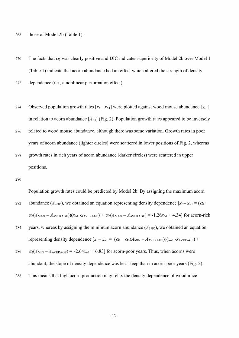
Population growth rates could be predicted by Model 2b. By assigning the maximum acorn

abundance (A2006), we obtained an equation representing density dependence [xt – xt-1 = (α1+282

α3(AMAX – AAVERAGE))(xt-1 -xAVERAGE) + α2(AMAX – AAVERAGE) = -1.26xt-1 + 4.34] for acorn-rich

years, whereas by assigning the minimum acorn abundance (A1996), we obtained an equation284

representing density dependence [xt – xt-1 = (α1+ α3(AMIN – AAVERAGE))(xt-1 -xAVERAGE) +

α2(AMIN – AAVERAGE) = -2.64xt-1 + 6.83] for acorn-poor years. Thus, when acorns were286

abundant, the slope of density dependence was less steep than in acorn-poor years (Fig. 2).

This means that high acorn production may relax the density dependence of wood mice.288

- 14 -

The region contained by the two lines in Fig. 2 represents the variation in density dependence290

generated by acorn abundance. If the variation in density dependence is completely explained

by acorn abundance, observed growth rates should be included in this region contained by the292

two lines. Indeed, most observed growth rates were located in the region (Fig. 2), indicating

that these predictions of Model 2b are valid.294

However, some unexpected predictions in this model were observed in the region to the left of296

the crossing point (Fig. 2). Assuming that acorn production was at its maximum and wood

mouse density (xt-1) was extremely low (e.g., x1996 = 0.003), the model predicts the population298

growth rate to be 4.34. On the other hand, assuming minimum acorn production with an

extreme low density of wood mouse, the population growth rate was predicted to be 6.82.300

Higher population growth rates should be predicted when acorns are abundant, if the mouse

density is the same. However, because the two lines cross at the point (

€

x − α2

α3

,

€

−α1α2

α3

),302

where

€

x is the mean abundance of wood mice, Model 2b yields unrealistically high

population growth rates when acorn production is poor and mouse density is low.304

To resolve these contradictory predictions, the nonlinear Ricker model (Model 3) was306

examined. Density dependence of wood mice and effects of acorn abundance were clearly

detected (Table 1). The mean α1 was 0.890, and the lower limit of the 95% CI was positive308

(0.430). The mean α2 was -0.199, and the higher limit of the 95% CI was negative (-0.041).

DIC indicates that Model 3 was the best model to represent wood mouse dynamics taking310

acorn effects in consideration.

312

- 15 -

Population growth rates predicted by Model 3 were plotted in Fig. 3. By assigning the

maximum and the minimum acorn abundance, we obtained an equation representing density314

dependence [xt - xt-1 = α0 - exp(α1(xt-1 -xAVERAGE) + α2(AMAX – AAVERAGE)) = 1.94 - exp(0.89xt-

1 - 3.00)] for acorn-rich years and [xt - xt-1 = α0 - exp(α1(xt-1 -xAVERAGE) + α2(AMIN – AAVERAGE))316

= 1.94 - exp(0.89xt-1 + 0.62)] for acorn-poor years, respectively.

318

Both curves gradually sloped down until around xt-1 = 2, which was close to the crossing point

of Model 2b, and when wood mouse density exceeded that density, the slopes of the curves320

became steeper. The curve for acorn-rich years was less steep than the curve for acorn-poor

years and was always located above. This also indicates that high acorn production may relax322

the density dependence of wood mice and then enhance the equilibrium density: i.e., acorn

abundance showed both “lateral” and “nonlinear perturbation” effects. In relation to the324

logistic model high acorn production enhances the carrying capacity (K).

326

In addition, these curves indicate that density effects are subtle at lower densities, while the

effects are emphasised at higher densities. This non-linearity means that higher densities have328

stronger effects on population growth rates.

330

Discussion332

A clear effect of acorn abundance was found consistently in all models that we examined

(Table 1). Comparing Model 1 with Model 2b, it is noteworthy that the interaction term (α3)334

between mice and acorns in Model 2b was clearly positive and that DIC indicated the

- 16 -

superiority of Model 2b over Model 1. These observations indicate that the interaction term is336

essential to describe the relationship between wood mice and acorn abundance. Moreover, the

fact that density dependence (α1) was emphasised in Model 2b means that acorn abundance338

influences the strength of density dependence. This is also shown by the fact that α3 can be

included in the term for xt-1 together with α1 in Model 2b.340

Royama (1992) conceptualised a density independent effect which shifts the equilibrium342

density to right or left, like the acorn effect in Model 1, as a “lateral perturbation effect” and a

different type of density independent effect which alters strength of density dependence, like344

the acorn effect in Model 2b as a “nonlinear perturbation effect”. He adduces nest holes for

birds as an example of a “lateral perturbation effect” and crops for birds as a “nonlinear346

perturbation effect”. Competition for nest holes can be characterised by a simple nest-to-bird

ratio, but consumption of crops cannot be measured by a simple crop-to-bird ratio, because348

the food is gradually depleted. Competition for crops may be more intense for the small

production of crops than for the large production. As a result the negative slope of population350

growth rates against density would become steeper for the small production than for the large

production. The present results based on Model 2b clearly demonstrate that acorn abundance352

acts as a “nonlinear perturbation effect” for density dependence of the wood mouse

population.354

Direct density dependence (α1) may be generated from intraspecific interactions for food or356

space in rodents. Although generalist predators are regarded as the main agents for direct

density dependence in Fennoscandia (Hansson and Henttonen 1988; Hanski et al. 2001;358

- 17 -

Turchin and Hanski 2001; Korpimäki et al. 2004), this is not the case for the Japanese wood

mouse because they are not preferred by predators in Hokkaido (Saitoh et al. 1999). There is360

some evidence suggesting intraspecific interactions in this species; density-dependent

reduction in reproduction related to territoriality has been observed (Kondo and Abe 1978).362

We therefore suggest that self-regulation through competition for space or food is the most

likely explanation of direct density dependence in the wood mouse in Hokkaido.364

Density dependence (α1) in Model 1 should be equivalent to [α1 + α3At-1] in Model 2b. When366

acorn abundance is at maximum, [α1 + α3At-1] is -1.26 in Model 2b. This value is very close to

α1 (-1.207) in Model 1. Thus, α1 in Model 1 may show the strength of density dependence in368

a condition without constraints of acorn abundance. In other words, although wood mice may

potentially be subject to very severe density dependence, density dependence is relaxed by an370

increase in acorn abundance.

372

Yoccoz et al. (2001) suggested that interactions between food and density may alter the

density-dependent structure. Although they expected that food availability would modify the374

slope of the regression between population growth rate and rodent density, they failed to find

such an effect of food availability on density dependence in bank vole (Clethrionomys376

glareolus) populations. Since bank voles are intermediate between herbivorous and

granivorous, and they consume a large variety of food items (Hanson 1985), the interactions378

between food and their abundance may be more complex.

380

- 18 -

Though our time series was rather short (16 years), it clearly showed that the strength of

density dependence of the wood mouse was altered by acorn abundance (Figs. 2 and 3). The382

diet of the wood mouse (genus Apodemus) is predominantly seeds and their abundance is

affected by seed availability (Flowerdew 1985; see also Montgomery 1989a, b; Montgomery384

and Montgomery 1990). Masting seeding improves reproduction and survival of Apodemus

(Montgomery et al. 1991; see Wilson et al. 1993 and Shimada and Saitoh 2006 for reviews).386

The two lines in Fig. 2 represent the range of variation in population growth rates, which is388

generated by variation in acorn abundance. The region contained by the two lines covers the

variation in the observed growth rates well when wood mouse density exceeds

€

x − α2

α3

. Model390

2b, however, yields unrealistic predictions under that density; population growth rates

predicted under acorn-poor conditions exceed those under acorn-rich conditions (Fig. 2).392

The nonlinear model (Model 3) resolves this problem (Fig. 3). The curve for acorn-rich years394

is always located above the curve for acorn-poor years and the fact that the curve for acorn-

rich years is less steep also demonstrates that acorn abundance has a “nonlinear perturbation396

effect” on density dependence of the wood mouse population. In addition, both curves

indicate that higher densities have stronger effects on population growth rates. This nonlinear398

nature of density dependence is also noteworthy.

400

Strong (1986) argued for the true existence of the nonlinearity of density dependence, and

Stenseth (1999) encouraged the investigation of questions “relating to the extent of402

nonlinearity and where in the interacting system such nonlinearity is located” to understand

- 19 -

the rodent cycle. Stenseth (1999) showed that the density-dependent structure during the404

increase phase differs from that during the decrease phase in the grey-sided vole in Finland

(see also Framstad et al. 1997; Stenseth et al. 1998). Lima et al. (2002a) found that density406

effects could be negligible below a threshold density in a shrew population.

408

The density of wood mice at for xt-1 = 2, from which density effects were emphasised, is

equivalent to 7-8 individuals per hectare in the study population. Home ranges of adult410

females of the wood mouse are spaced apart, and the home range size is 604–962 m2 during

the breeding season; in contrast, those of adult males overlap with each other and with those412

of females, and are 858–1853 m2 during the breeding season (Oka 1992). Since 1 ha (10,000

m2) is sufficiently large for 7-8 females to establish exclusive home ranges, intraspecific414

competition may be minor below this density level.

416

We have found that the strength of density dependence was altered by acorn abundance, and

we have demonstrated the nonlinearity of density dependence of the wood mouse population.418

We make the following suggestions for further studies on density dependence in rodent

populations, dynamics of wood mouse populations, and rodent-seed interactions:420

1. In contrast to our results, Yoccoz et al. (2001) concluded that the effects of food on

density dependence are negligible in the bank vole (Clethrionomys glareolus). Our422

results suggest that wood mice compete for acorns, whereas direct density dependence

of bank vole populations may not be generated by competition for food, but for other424

resources. Generalist predators may be agents for direct density dependence of the

- 20 -

bank vole. Comparative studies on density-dependent mechanisms between Apodemus426

and Clethrionomys would therefore be of interest.

2. We have demonstrated nonlinearity in density dependence. Density effects are minor428

at low-density levels. We recommend comparing space use and dispersal patterns of

wood mice between low- and high-density conditions.430

3. The nonlinear model in Fig. 3 does not perfectly represent the observed variation in

population growth rates. Since the model consists of variables in the previous year (t -432

1), the variation that derives from effects in the current year (t) is not covered. Studies

on food resources or other factors in the current year that influence the reproduction of434

the wood mouse should be conducted. In addition information under low density

conditions which is scarce in this study should be accumulated. The model would be436

revised using such information.

438

Acknowledgements440

We are indebted to the staff of the Uryu Experimental Forest, Field Science Centre, Hokkaido

University, for providing support for the investigation. Takuya Shimada and Gaku Takimoto442

critically read the manuscript and provided helpful comments. Takuya Kubo and Kohji

Yamamura also gave us helpful comments on statistical analyses. Sandy Liebhold and444

anonymous reviewers greatly contributed to improving the manuscript. Ed Dyson assisted in

editing the manuscript. This research was partially supported by a Ministry of Education,446

Science, Sports, Culture and Technology Grant-in-Aid for Scientific Research (B), No.

19370006 and No. 1938009117 to TS.448

- 21 -

References450

Abe H (1986) Vertical space use of voles and mice in woods of Hokkaido, Japan. J Mammal

Soc Japan 11: 93-106452

Animal Care and Use Committee (1998) Guidelines for the capture, handling, and care of

mammals as approved by the American Society of Mammalogists. J Mammal 79: 1416-454

1431

Batzli G (1992) Dynamics of small mammal populations: a review. In: DR McCullough, RD456

Barrett (eds.), Wildlife 2001: Populations. Elsevier, London, pp. 831-850

Bjørnstad ON, Falck W, Stenseth NC (1995) A geographic gradient in small rodent density458

fluctuations: a statistical modelling approach. Proc R Soc Lond B 262:127-133

de Valpine P, Hastings A (2002) Fitting population models incorporating process noise and460

observation error. Ecol Monogr 72:57-76

Flowerdew JR (1985) The population dynamics of wood mice and yellow-necked mice. Symp462

Zool Soc Lond 55: 315-338

Framstad E, Stenseth NC, Bjørnstad ON, Falck W (1997) Limit cycles in Norwegian464

lemmings: tensions between phase-dependence and density-dependence. Proc R Soc

Lond B 264: 127-133466

Fujimaki Y (1969) The fluctuations in the number of small rodents. Bull Hokkaido For Exp

Stn 7:62-77 (in Japanese with English summary)468

Jensen TS (1982) Seed production and outbreaks of non-cyclic rodent populations in

deciduous forests. Oecologia 54:184-192470

Hanski I, Henttonen H, Korpimäki E, Oksanen L, Turchin P (2001) Small-rodent dynamics

- 22 -

and predation. Ecology 82:1505–1520472

Hansson L (1985) Clethrionomys food: generic, specific and regional characteristics. Ann

Zool Fenn 22:315-318474

Hansson L, Henttonen H (1988) Rodent dynamics as community processes. Trends Ecol Evol

3:195-200476

Klemola T, Pettersen T, Stenseth NC (2003) Trophic interactions in population cycles of voles

and lemmings: a modelling study and a review-synthesis. Adv Ecol Res 33:75-160478

Kondo N, Abe H (1978) Reproductive activity of Apodemus speciosus ainu. Memoirs Fac Agr

Hokkaido Univ 11:159-165 (in Japanese with English summary)480

Korpimäki E, Brown PR, Jacob J, Pech R (2004) The puzzles of population cycles and

outbreaks of small mammals solved? BioScience 54:1071-1079482

Krebs CJ (1999) Ecological methodology. Benjamin/Cummings, Menlo Park. 620pp

Lima M, Julliard R, Stenseth NC, Jaksic FM (2001) Demographic dynamics of a neotropical small484

rodent (Phyllotis darwini): feedback structure, predation and climatic factors. J Anim

Ecol 70:761-775486

Lima M, Merritt JF, Bozinovic F (2002a) Numerical fluctuations in the northern short-tailed

shrew: evidence of non-linear feedback signature on population dynamics and488

demography. J Anim Ecol 71:159-172

Lima M, Stenseth NC, Jaksic FM (2002b) Food web structure and climate effects on the490

dynamics of small mammals and owls in semi-arid Chile. Ecol Lett 5:273-284

Lima M, Berryman AA, Stenseth NC (2006) Feedback structures of northern small rodent492

populations. Oikos 112:555-564

Mallorie HC, Flowerdew JR (1994) Woodland small mammal population ecology in Britain:494

- 23 -

a preliminary review of the Mammal Society survey of wood mice Apodemus sylvaticus

and bank voles Clethrionomys glareolus, 1982-87. Mammal Rev 24:1-15496

Miguchi H (1988) Two years of community dynamics of murid rodents after a beechnut

mastyear. J Jpn For Soc 70:472-480 (in Japanese with English summary)498

Miyaki M, Kikuzawa K (1988) Dispersal of Quercus mongolica acorns in a broadleaved

deciduous forest. 2. Scatterhoarding by mice. For Ecol and Manage 25:9-16500

Montgomery WI (1989a) Population regulation in the wood mouse Apodemus sylvaticus I.

Density dependence in the annual cycle of abundance. J Anim Ecol 58:465-476502

Montgomery WI (1989b) Population regulation in the wood mouse Apodemus sylvaticus II.

Density dependence in spatial distribution and reproduction. J Anim Ecol 58:477-494.504

Montgomery SSJ, Montgomery WI (1990) Intrapopulation variation in the diet of the wood

mouse Apodemus sylvaticus. J Zool 222:641-651506

Montgomery WI, Wilson WL, Hamilton R, McCartney P (1991) Dispersion in the wood

mouse, Apodemus sylvaticus: variable resources in time and space. J Anim Ecol 60:179-508

192

Murakami O (1974) Growth and development of the Japanese wood mouse (Apodemus510

speciosus). I. The breeding season in the field. Jpn J Ecol 24:194-206 (in Japanese with

English summary)512

Murúa R, González LA, Lima M (2003) Population dynamics of rice rats (a Hantavirus

reservoir) in southern Chile: feedback structure and no-linear effects of climatic514

oscillations. Oikos 102:137-145

Oka T (1992) Home range and mating system of two sympatric field mouse species,516

Apodemus speciosus and Apodemus argenteus. Ecol Res 7:163-169

- 24 -

Ota K (1968) Studies on the ecological distribution of the murid rodents in Hokkaido. Res518

Bull Coll Exp For (Fac Agr Hokkaido Univ) 26:223-295 (in Japanese with English

summary)520

Prévot-Julliard A-C, Henttonem H, Yoccoz NG, Stenseth NC (1999) Delayed maturation in

female bank voles: optimal decision or social constraints? J Anim Ecol 68:684-697522

Royama T (1992) Analytical population dynamics. Chapman and Hall, London.

Saitoh T, Stenseth NC, Bjørnstad ON (1997) Density dependence in fluctuating grey-sided524

vole populations. J Anim Ecol 66:14-24

Saitoh T, Bjørnstad ON, Stenseth NC (1999) Density-dependence in voles and mice: a526

comparative study. Ecology 80:638-650

Saitoh T, Osawa J, Takanishi T, Hayakashi S, Ohmori M, Uemura S, Vik JO, Stenseth NC,528

Maekawa K (2007) Effects of acorn masting on population dynamics of three forest-

dwelling rodent species in Hokkaido, Japan. Popul Ecol 49:249-256530

Sekijima T, Soné K (1994) Role of interspecific competition in the coexistence of Apodemus

argenteus and A. speciosus (Rodentia: Muridae). Ecol Res 9:237-244532

Shimada T (2001) Nutrient compositions of acorns and horse chestnuts in relation to seed-

hoarding. Ecol Res 16:803-808534

Shimada T, Saitoh T (2006) Re-evaluation of the relationship between rodent populations and

acorn masting: a review from the aspect of nutrients and defensive chemicals in536

acorns. Popul Ecol 48:341-352

Soné K, Kohno A (1996) Application of radiotelemetry to the survey of acorn dispersal by538

Apodemus mice. Ecol Res 11:187-192

Spiegelhalter DJ, Thomas A, Best NG, Lunn D (2003) WinBUGS user manual (version 1.4).540

- 25 -

MRC Biostatistics Unit, Institute of Public Health, Cambridge

Stenseth NC (1999) Population cycles in voles and lemmings: density dependence and phase542

dependence in a stochastic world. Oikos 87:427-461

Stenseth NC, Bjørnstad ON, Falck W (1996). Is spacing behaviour coupled with predation544

causing the microtine density cycle? A synthesis of process-oriented and pattern-

oriented studies. Proc R Soc Lond B 263:1423-1435546

Stenseth NC, Chan K-S, Framstad E, Tong H (1998) Phase- and density-dependent

population dynamics in Norwegian lemmings: interaction between deterministic and548

stochastic processes. Proc R Soc Lond B 265:1957-1968

Stenseth NC, Viljugrein H, Saitoh T, Hansen TF, Kittilsen MO, Bølviken E, Glöckner F550

(2003) Seasonality, density dependence and population cycles in Hokkaido voles. Proc

Natl Acad Sci USA 100:11478-11483552

Strong DR (1986) Density-vague population change. Trends Ecol Evol 1:39-42

Turchin P (2003) Complex population dynamics: A theoretical/empirical synthesis. Princeton554

University Press, Princeton.

Turchin P, Hanski I (2001) Contrasting alternative hypotheses about cycles by translating556

them into parameterised models. Ecol Lett 4:267–276

Viljugrein H, Stenseth NC, Smith GW, Steinbakk GH (2005) Density dependence in North558

American ducks. Ecology 86:245-254

Wilson WL, Montgomery WI, Elwood RW (1993) Population regulation in the wood mouse560

Apodemus sylvaticus (L.). Mammal Rev 23:73-92

Yoccoz NG, Stenseth NC, Henttonen H, Prévot-Julliard A-C (2001) Effects of food addition562

on the seasonal density-dependent structure of bank vole Clethrionomys glareolus

- 26 -

populations. J Anim Ecol 70:703-720564

566

568

- 27 -

Table 1. Estimated coefficients of each model. Density effects of wood mice (α1), direct effect of acorn abundance (α2), interaction between570

wood mice and acorns (α3), and a constant (α0) are shown. SD and 95% CI indicate standard deviation and 95% credible interval, respectively.

DIC (Deviance Information Criterion) is a Bayesian method for model comparison.572

α0 α1 α2 α3

mean SD 95% CI mean SD 95% CI mean SD 95% CI mean SD 95% CI DICModel 1 -1.207 0.233 [-1.662,

-0.738]0.366 0.132 [0.109,

0.635]339.4

Model 2a -1.739 0.335 [-2.466,-1.127]

0.342 0.099 [0.150,0.544]

0.288 0.124 [0.050,0.546]

337.8

Model 2b -1.747 0.359 [-2.543,-1.119]

0.342 0.103 [0.148,0.555]

0.287 0.124 [0.051,0.544]

334.7

Model 3 1.944 0.741 [0.355,3.343]

0.890 1.130 [0.430,2.954]

-0.199 0.232 [-0.644,-0.041]

321.3

574

- 28 -

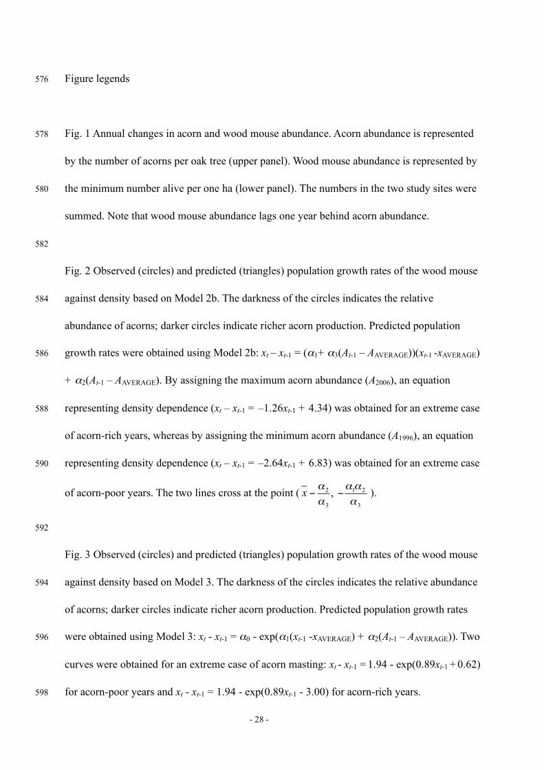
Figure legends576

Fig. 1 Annual changes in acorn and wood mouse abundance. Acorn abundance is represented578

by the number of acorns per oak tree (upper panel). Wood mouse abundance is represented by

the minimum number alive per one ha (lower panel). The numbers in the two study sites were580

summed. Note that wood mouse abundance lags one year behind acorn abundance.

582

Fig. 2 Observed (circles) and predicted (triangles) population growth rates of the wood mouse

against density based on Model 2b. The darkness of the circles indicates the relative584

abundance of acorns; darker circles indicate richer acorn production. Predicted population

growth rates were obtained using Model 2b: xt – xt-1 = (α1+ α3(At-1 – AAVERAGE))(xt-1 -xAVERAGE)586

+ α2(At-1 – AAVERAGE). By assigning the maximum acorn abundance (A2006), an equation

representing density dependence (xt – xt-1 = –1.26xt-1 + 4.34) was obtained for an extreme case588

of acorn-rich years, whereas by assigning the minimum acorn abundance (A1996), an equation

representing density dependence (xt – xt-1 = –2.64xt-1 + 6.83) was obtained for an extreme case590

of acorn-poor years. The two lines cross at the point (

€

x − α2

α3

,

€

−α1α2

α3

).

592

Fig. 3 Observed (circles) and predicted (triangles) population growth rates of the wood mouse

against density based on Model 3. The darkness of the circles indicates the relative abundance594

of acorns; darker circles indicate richer acorn production. Predicted population growth rates

were obtained using Model 3: xt - xt-1 = α0 - exp(α1(xt-1 -xAVERAGE) + α2(At-1 – AAVERAGE)). Two596

curves were obtained for an extreme case of acorn masting: xt - xt-1 = 1.94 - exp(0.89xt-1 + 0.62)

for acorn-poor years and xt - xt-1 = 1.94 - exp(0.89xt-1 - 3.00) for acorn-rich years.598

Figure 1

1992 1994 1996 1998 2000 2002 2004 2006

0

20

40

60

80

Woo

d m

ouse

abu

ndan

ce

1991 1993 1995 1997 1999 2001 2003 20050

1000

2000

3000

4000A

corn

abu

ndan

ce

Figure 2

-6

-4

-2

0

2

4

6

8

1 2 3 4 5

t t-1 1 3 t-1 t-1 2 t-1x - x = (α + α (A - A ))(x - x ) + α (A - A )

t-1Abundance (x )

Popu

latio

n G

row

th R

ate

(x -

x

)t

t-1

Figure 3

-6

-4

-2

0

2

4

6

8

0 1 2 3 4 5

Popu

latio

n G

row

th R

ate

(x -

x

)t

t-1 t t-1 0 1 t-1 2 t-1x - x = α - exp(α (x - x ) + α (A - A ))

t-1Abundance (x )