Introduction(2007/09/04) - 筑波大学rhodia.ph.tsukuba.ac.jp/~hatsugai/modules/pico/PDF/lectures/... · Introduction(2007/09/04) Geometric phase Quantum liquid ... No symmetry breaking

Condensed matter physics lecture notes

JiYoung Kang

Dept. Physics, Tsukuba University(Dated: Nov/29/2007)

Part I

Introduction(2007/09/04)Geometric phase

Quantum liquid

� Quantum Hall system

� Quantum Super conductor

� Kondo insulator

� 1-dimension integer spin chain

� Materials with strong correlationSpin systems with frustrationdimers

� No symmetry breaking ( Symmetry breaking is no more important )

What is the Phase ?Ans) State of matters. In physics, we need quantitative analysis to describe system. To describe phase transition, weuse order parameter.

(Ex) FerromagnetsLet us de�ne local magnetization ~m(~r) as a direction of magnetization at ~r. In ferromagnets, ~m(~r) independent ~r.Then, the correlation length is in�nity. It represents that ferromagnet has long range order. Changing of local orderparameter to long range order parameter, one can see the phase change.

Spontaneous Symmetry breakingLocally, the system has no directional property. But, many particles (size of system!1) makes directional properties.(i.e.) Micro system which has symmetry. But sum of micro system, macro system has no more this symmetry.[Spontaneous(it need not existence of external magnetic �eld) symmetry breaking]First, let us assume one �nite system which has external magnetic �eld ~B 6= 0(There are some special direction.). Ifone reduce the external magnetic �elds, then symmetry will be recover. Let us think two ways of limit,(a) ~B ! 0 =) N !1 [it is not ferromagnets](b) N !1 =) ~B ! 0 [it is a ferromagnet](a) and (b) are not equivalent.

Examples of spontaneous symmetry breaking : Ferromagnets, super conductorSpontaneous symmetry breaking(order phase)

Existence of long distance order is not always same to Spontaneous symmetry breaking.[Existence of long distance order�Spontaneous symmetry breaking]

Order parameter gives the phase. Phase transition = phenomena of changing phase.

Lecture given by Y. Hatsugai at U. Tsukuba 2007 ( Note taken by J. Kang)

Classical phase transition : In low temperature, system has order, temperately �uctuation is down. It relatedcompetition of entropy and stabilization energy.Quantum phase transition (QPT): Transition as changing of physical parameter near the zero temperature.

(example of QPT)

Mott transition (Metal-insulator) : In low temperature, changing of electron correlation or doping, metal becomeinsulator! In this case, order parameter is not clear. (Naively electricity conduction)Transition of plate in the Quantum Hall system :

Hall conduction

�xy = (integer)�e2

h

In this transition, integer change.Change of Intensity of disorder , magnetic �eld (�lling)

Quantum liquidsNo symmetry breakingNo classical order parameter(ex) Transition in Quantum Hall systemNon-isotopic superconducts ( Breaking of U(1) symmetry ) - there are some classes of superconductor.

Geometrical phase(Important part of Quantum e¤ect ) ! Distinguish Quantum liquids

(example of quantum liquids)Kondo insulator (strong-correlation matter)

Kondo e¤ect : loss of spin by quantum e¤ect.1-dimension : polyacetylene - strength of bonding is changing [If 1 lattice point has 1 electron, the it become insulator]2-dimension : graphen - e¤ective mass approximation is no more established. When conduction band and valence

band meet one point, energy E � c��~k��, and it become Dirac fermions (it follows Dirac equation).

Part II

Quantum Hall e¤ects (2007/09/11)(picture) Two dimension electron gas. Ix = �xyVy; �xy:quantize.

�xy = integer ! integer Q.H.E.(Quantum Hall E¤ect)

= p=q ! fractional Q.H.E.

(p:q) = 1 mutually prime integers. Mostly q is odd. q is even in denominator state.

I. CLASSICAL DESCRIPTION

Charged particles in an electromagnetic �ledEquation of motion ?Lorentz force is given by

m::

~r = e( ~E + ~v � ~B);

where, m : mass

e : charge~B : magnetic �eld~E : Electric �eld

~r (t) : position of particle

2


Time t change ti ! tf . f~r (t)g is world line. In classical electromagnetism, we introduce potentials ~A; �.

~E = �@~A

@t�r�

~B = r� ~A

In component representation,

Ei = �@~A

@t� @i�;

Bi = "ijk@jAk;

where i = x; y; z:Rewriting motion of equation,

m::ri = e (�@0Ai � @i�+ "ijkvj"klm@lAm)= e (�@0Ai � @i�+ "kijvj"klm@lAm)= e (�@0Ai � @i�+ (�il�jm � �im�jl) vj@lAm)= e (�@0Ai � @i�+ vj@iAj � vj@jAi) :

To smoothly quantization, let think principle of least action. Action is given by

S [~r] =

Z t2

t1

dtL�~r (t) ;

:

~r (t)�;

where L indicate Lagrangian. Following principle of least action,

�S = 0 , Newton equation of motion.

One suggestion of Lagrangian is

L =1

2m:

~r2� e� (r (t) ; t) +

:

~r � ~A (~r (t) ; t) :

Let us check this Lagrangian. �S = 0 give us Euler-Lagrange equation,

d

dt

@L

@ _ri� @L

@ri= 0:

Substituting this Lagrangian,

@L

@ri= �e@i�+ e _rj � @iAj ;

@L

@ _ri= m _ri + eAi (~r (t) ; t) ;

d

dt

@

@ _ri= m

::ri + e ( _rj@jAi + @0Ai) :

Then, Euler-Lagrange equation is given by

d

dt

@L

@ _ri� @L

@ri= m

::ri + e ( _rj@jAi + @0Ai)� f�e@i�+ e _rj � @iAjg

= 0;

m::ri = e (�@0Ai � @i�+ e _rj � @iAj � _rj@jAi) :

This result is agreement with Newton equation.

3


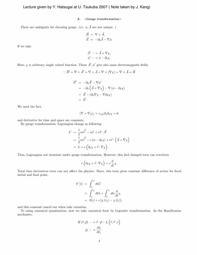
A. <Gauge transformation>

There are ambiguity for choosing gauge. (i.e. �; ~A are not unique. )

~B = r� ~A;

~E = �@0 ~A�r�:

If we take

~A0 : = ~A+r�;�0 : = �� @0�:

Here, � is arbitrary single valued function. These ~A0; �0 give also same electromagnetic �elds.

* ~B0 = r� ~A0 = r� ~A+r� (r�) = r� ~A = ~B

~E0 = �@0 ~A0 �r�0

= �@0�~A+r�

��r (�� @0�)

= ~E � (@0r��r@0�)= ~E:

We used the fact,

(r�r�)i = "ijk@j@k� = 0;

and derivative for time and space are commute.By gauge transformation, Lagrangian change as following

L0 =1

2m:

~r2� e�0 + e

:

~r � ~A0

=1

2m:

~r2� e (�� @0�) + e

:

~r ��~A+r�

�= L+ e

�@0�+

:

~r � r��:

Thus, Lagrangian not invariant under gauge transformation. However, this 2nd changed term can rewritten

e�@0�+

:

~r � r��= e

d

dt�:

Total time derivatives term can not a¤ect the physics. Since, this term gives constant di¤erence of action for �xedinitial and �nal point,

S0 [r] =

Z tf

ti

dtL0

=

Z tf

ti

dtL+

Z tf

ti

dted

dt�

= S[r] + e [� (tf )� � (ti)] ;

and this constant cancel out when take variation.To using canonical quantization, now we take canonical form by Legendre transformation. In the Hamiltonian

mechanics,

H (~r; ~p) : =:

~r � ~p� L�~r;

:

~r ; t�

~pi : =@L

@ _ri

4


(cf.) H (~r; ~p) is independent for:

~r ? ANS. yes!

* �H = �:

~r � ~p+:

~r�~p� �r � @L@~r

� �:

~r@L

@:

~r

= �:

~r ��~p� @L

@:

~r

�+

:

~r�~p� �r � @L@~r

=:

~r�~p� �r � @L@~r:�H is independent of

:

~r�

The Hamiltonian equation is given by

@H

@p=

:

~r

@H

@~r= �

:

~p:

Because,

@H

@~p=

:

~r;

@H

@~r= �@L

@~r= � d

dt

@L

@:

~r= �

:

~p:

In electromagnetic system,

L�~r;

:

~r ; t�=1

2m:

~r2� e�+ e

:

~r � ~A

~p =@L

@:

~r= m

:

~r + e ~A

:

~r =1

m

�~p� e ~A

�:

Under gauge transformation,

L0 = L+ e�@0�+

:

~rr��

~p0 =@L

@:

~r+ er�

= ~p+ er�: (Not invariant !)

This canonical momentum is not invariant under gauge transformation, but mechanical momentum is invariant ::

~r0 =1

m

�~p0 � e ~A0

�=

1

m

�~p+ er�� e

�~A+r�

��=

:

~r +1

m(er�� er�)

=:

~r:

The Hamiltonian is

H =:

~r � ~p� L�~r;

:

~r ; t�

=:

~r ��m:

~r + e ~A��1

2m:

~r2� e�+ e

:

~r � ~A�

=1

2m

:

~r2 + e�

=1

2m

�~p� e ~A

�2+ e�:

5


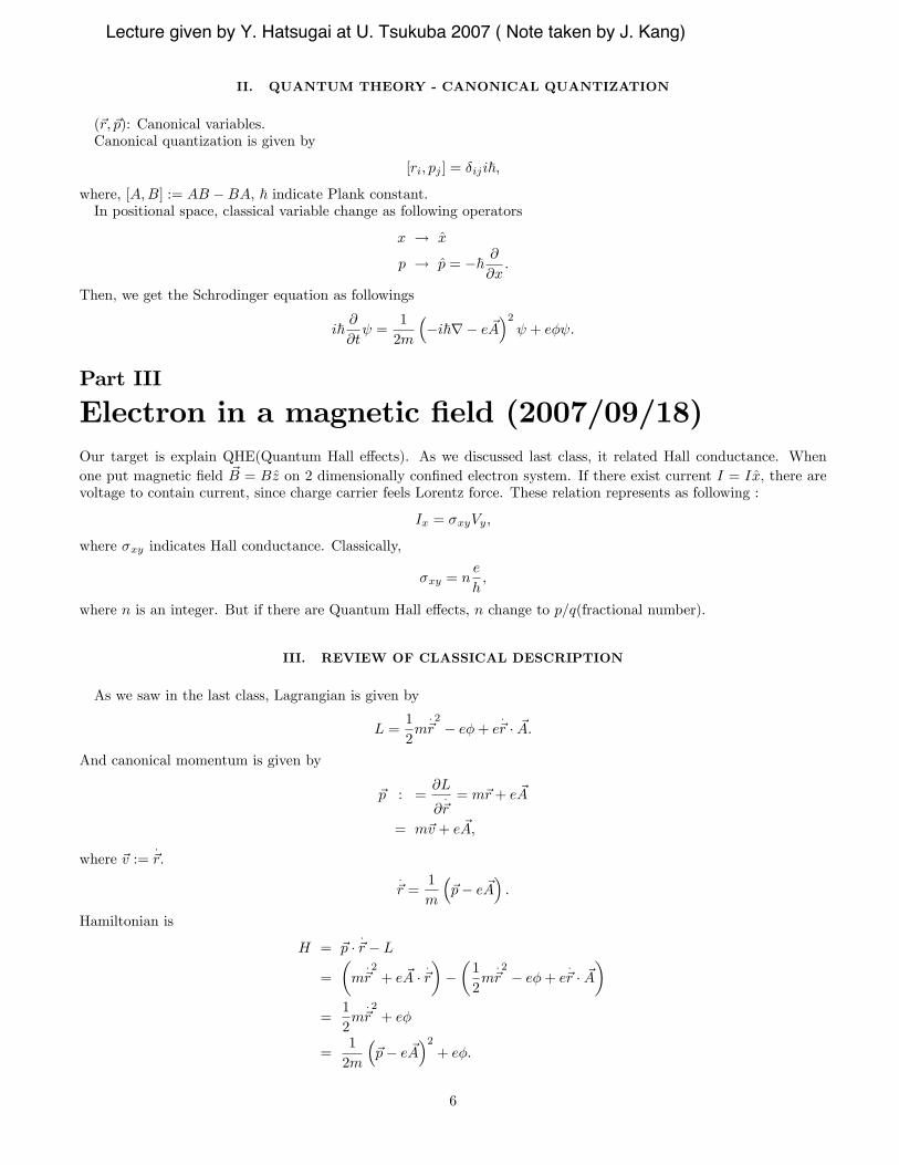
II. QUANTUM THEORY - CANONICAL QUANTIZATION

(~r; ~p): Canonical variables.Canonical quantization is given by

[ri; pj ] = �iji~;

where, [A;B] := AB �BA, ~ indicate Plank constant.In positional space, classical variable change as following operators

x ! x

p ! p = �~ @@x:

Then, we get the Schrodinger equation as followings

i~@

@t =

1

2m

��i~r� e ~A

�2 + e� :

Part III

Electron in a magnetic �eld (2007/09/18)Our target is explain QHE(Quantum Hall e¤ects). As we discussed last class, it related Hall conductance. Whenone put magnetic �eld ~B = Bz on 2 dimensionally con�ned electron system. If there exist current I = Ix, there arevoltage to contain current, since charge carrier feels Lorentz force. These relation represents as following :

Ix = �xyVy;

where �xy indicates Hall conductance. Classically,

�xy = ne

h;

where n is an integer. But if there are Quantum Hall e¤ects, n change to p=q(fractional number).

III. REVIEW OF CLASSICAL DESCRIPTION

As we saw in the last class, Lagrangian is given by

L =1

2m:

~r2� e�+ e

:

~r � ~A:

And canonical momentum is given by

~p : =@L

@:

~r= m~r + e ~A

= m~v + e ~A;

where ~v :=:

~r.:

~r =1

m

�~p� e ~A

�:

Hamiltonian is

H = ~p �:

~r � L

=

�m:

~r2+ e ~A �

:

~r

��1

2m:

~r2� e�+ e

:

~r � ~A�

=1

2m:

~r2+ e�

=1

2m

�~p� e ~A

�2+ e�:

6


(comment)

~j = e:

~r

=@L

@ ~A

= �@H@ ~A

= � 1m

�~p� e ~A

�(�e) :

IV. REVIEW OF QUANTUM DESCRIPTION

Using canonical quantization,

[r�; p� ] = i~�� ;

and in position space, momentum operator is given by

~p =~ir;

we can write Schrodinger equation

i~@

@t= H (~r; ~p)

= H

�~r;~ir� ;

where (~r; t) is a wave function.

V. GAUGE TRANSFORMATION & CONSERVED CURRENT(SPIN HALL EFFECT)

(Comment) Laughlim argument : essence of the QHE.As well known Nother theory, symmetry gives conserved property.We will see that the probability of density is conserved as in the level of quantum mechanics.First, similarly to classical mechanics, we de�ne current density as

~j0 : = �e~v

=e

m ��~p� e ~A

�

=e

m ��~ir� e ~A

� :

Integrate for all space, Zd~r ~j0 =

Zd~r

e

m ��~ir� e ~A

�

=

Zd~r

e

m �~ir �

Zd~re2

m~A j j2

=

Zd~re~mi

[r ( � )� (r �) ]�Zd~re2

m~A j j2

=

�e~mi

( � )

�surface

�Zd~re~mi

(r �) �Zd~re2

m~A j j2

= �Zd~re~mi

(r �) �Zd~re2

m~A j j2 :

Also we can take

~j00 := e~v �:

7


And, to make well de�ned current we now de�ne current density as following :

~j : =1

2

�~j0 +~j00

�=

~e2mi

((r ) � � (r �) )� e2 ~A

mj j2 : (1)

Charge density is given by

� (~r) = e j (~r)j2 = e � ;

where j (~r)j2 is a probability density of the particle at ~r. Di¤erentiating � (~r) by time t, we get@�

@t= e

�@ �

@t + �

@

@t

�: (2)

Using the Schrodinger equation,

@

@t=

1

i~

"1

2m

�~ir� e ~A

�2 + e�

#

=1

i~

�1

2m

�~ir� e ~A

��~ir� e ~A

� + e�

�=

1

i~

"1

2m

�~ir�2� ~i

nr ��e ~A�o� 2~

ie ~Ar+ e2 ~A2

! + e�

#;

and its complex conjugate

@ �

@t=�1i~

"1

2m

��~ir� e ~A

�2 � + e� �

#

=�1i~

"1

2m

�~ir�2+~i

nr ��e ~A�o+2~ie ~Ar+ e2 ~A2

! � + e� �

#;

we can rewrite (Eq. 2) as

@�

@t=

e

i~ �

"1

2m

�~ir�2� ~i

nr ��e ~A�o� 2~

ie ~Ar+ e2 ~A2

! + e�

#

� e

i~

"1

2m

�~ir�2+~i

nr ��e ~A�o+2~ie ~Ar+ e2 ~A2

! � + e� �

#

=e

i~ �

"1

2m

�~ir�2� ~i

nr ��e ~A�o� 2~

ie ~Ar

!

#

� e

i~

"1

2m

�~ir�2+~i

nr ��e ~A�o+2~ie ~Ar

! �

#

=e

i~1

2m

" ��~ir�2

� �~ir�2

� � 2~ie ~A ( �r + r �)� 2~

i

nr ��e ~A�oj j2

#

=�ei~

1

2m

�~2� � (r)2 � (r)2 �

�+2~ie ~A ( �r + r �) + 2~

i


�=�ei~

1

2m

�~2r � ( � (r )� (r �)) + 2~

ie ~Ar � ( � ) + 2~

i


�=�ei~

1

2m

�~2r � ( � (r )� (r �)) + 2~

ie ~Ar � ( � ) + 2~

i


�=�ei~

1

2m

�~2r � ( � (r )� (r �)) + 2~

ier �

�~A �

��= �r �

�~e2mi

( � (r )� (r �))� e

m

�~A �

��:

8


From the de�nition of current density (Eq. 1),

~j =~e2mi

((r ) � � (r �) )� e2 ~A

mj j2 ;

we �nally get equation of continuity,

@�

@t= �r �~j:

It represents conservation of probability.

Part IV

(2007/09/25)VI. REVIEW

i~@

@t = H;

where,

H =1

2m

�~p� e ~A

�2+ e�;

~p =~ir:

Density � = e j j2

Density current ~j = eh~2m (

�r � (r �) )� em~A j j2

iConservation law @0�+r �~j = 0:

VII. GAUGE TRANSFORMATION

Let us see gauge transformation in quantum mechanical system.Gauge transformation

~A ! ~A0 = ~A+r�

� ! �0 = �� @�

@t

where � is a single valued function. In gauge transformation, Hamiltonian and wave function will be changed.Assume local gauge transformation form,

0 (~r; t) = ei�(~r;t) (~r; t) ;

this condition represents the phase is arbitrary at each point of space-time. (Gauge symmetry) Then,

(~r; t) = e�i�(~r;t) 0 (~r; t) ;

and we see that �~p� e ~A

� =

��i~r� e ~A

�e�i� 0

= (�i~) (�ir�) e�i� 0 + (�i~) e�i�r 0 � e ~A e�i� 0

= e�i�h�~r� � i~r� e ~A

i 0

= e�i��i~r� e

�~A+

~er��

0

= e�i�h~p� e ~A0

i 0;

9


last line I de�ned ~A0 := ~A+ ~er�; (� :=

e~�):

Since �~p� e ~A

�2 =

�~p� e ~A

��~p� e ~A

�

=�~p� e ~A

�ne�i�

h~p� e ~A0

i 0o

= e�i��~p� e ~A0

�2 0:

Recalling 0 = ei� ,

i~@

@t = i~

@

@t

�e�i� 0

�= i~ (�i)

�@�

@t

� 0 + i~e�i�

@

@t 0

= ~@�

@t 0 + i~e�i�

@

@t 0:

Then, the Schrodinger equation,

i~@

@t =

�1

2m

�~p� e ~A

�2+ e�

� ;

= e�i� 0;

~@�

@t 0e�i� + i~e�i�

@

@t 0 =

e�i�

2m

�~p� e ~A0

�2 0 + e�e�i� 0;

multiplying ei�,

i~@ 0

@t=

�1

2m

�~p� e ~A0

�2 0 + e� 0 � ~@�

@t 0�

=

�1

2m

�~p� e ~A0

�2+ e

�� ~

e

@�

@t

�� 0

=

�1

2m

�~p� e ~A0

�2+ e

�� @�

@t

�� 0

=

�1

2m

�~p� e ~A0

�2+ e�0

� 0

= H 0 0:

Summarizing these,

~A ! ~A0 = ~A+r�

� ! �0 = �� @�

@t

! 0 = ei�

H ! H 0 =1

2m

�~p� e ~A0

�2+ e�0

i~@

@t= H

i~@ 0

@t= H 0 0

we see that Schrodinger equation is covariant. Observables like density of probability or density current need toinvariant. Let us con�rm these, density of probability is clearly,

�! �0 =�� 0��2 = j j2 :10


~j ! ~j0 = e

�~2mi

� 0�r 0 �

�r 0�

� 0�� e

m~A0�� 0��2�

~j0 = e

�~2mi

� �r � (r �) + 2ir� j j2

�� e

m

�~A+r�

�j j2

�= ~j + e�

�~2mi

2ir� � e

mr��

= ~j:

Thus, conservation law is conserved

@�0

@t+r0 �~j = 0:

! 0 = eie~�

= ei2�e~�

: = ei2��0 ;

where �0 := he is called �ux quantum.

Dimensional analysis of ~A : From

~A! ~A0 = ~A+r�;

~B = r� ~A; :

we see magnetic �eld and � has following dimensional relation:

[B] � [�]

[L2];

� � B�L2�� ux

� � �0 [mod �0] :

<Example> Let us assume that there exist uniform magnetic �eld ~B = r� ~A = (0; 0; B)(time independent) with~E = 0.Gauge choice 1.Landau gauge � = 0; ~AL = (0; xB; 0)Gauge choice 2.Symmetric gauge � = 0; ~AS = 1

2 (yB;�xB; 0)Both gauges give us

~B = r� ~A = (0; 0; B) :

In steady state, we can separate variables,

(r; t) = e�i!t (~r) ;

and we have

i~@

@t= H ;

de�ning E := ~!; we see that

~! = E:

Using Landau gauge,

1

2m

�~p� e ~AL

�2 =

1

2m

"�~2 @

2

@x2+

��i~ @

@y+ eBx

�2� ~2 @

@z2

# = E :

11


Inserting

= eikyyeikzz� (x) ;

we have

1

2m

�~p� e ~AL

�2 =

1

2m

h�~2�00 + (~ky + eBx)2 �+ ~2k2z�

ieikyyeikzz:

De�ning

E2D = E � ~2k2z2m

;

we can compare harmonics oscillator

~2

2m

�� d2

dx2+�ky +

e

~Bx�2�

� = E2D�; (3)

� ~2

2m

d2

dx2+1

2m!2x2: cf. Harmonic oscillator.

Putting

X = x+~eB

ky;

d

dX=

d

dx;

(Eq. 3) is given by "� ~

2

2m

d2

dx2+~2

2m

e2B2

~2

�x+

~eB

ky

�2#� = E2D�;�

� ~2

2m

d2

dx2+m

2

e2B2

m2X2

�� = E2D�:

So,

! =

�eB

m

�is called as cycrotron frequency. And E2D is quantize, it called Landau levels,

E2D =1

2~!�n+

1

2

�;

n = 0; 1; 2; ::::

X = x+~kyeB

=: x+ l kyl;

note that kyl is dimensionless.

l2 =~eB

;

l =

r~eB

: magnetic length.

note that magnetic length has a unique length scale, ~! energy scale.If there exists O 6= 0 Hermit operator which satis�ed

12


[H;O] = 0;

then there exist conserved quantity. (Landau degeneracy)

Part V

(2007/10/02)VIII. 2 DIMENSIONAL ELECTRON PROBLEM IN A UNIFORM MAGNETIC FIELD

Hamiltonian is given by

H =1

2m

�~p� e ~A

�2=

1

2m

h(px � eAx)2 + (py � eAy)2

i=

1

2m~�2;

where, ~� = (�x;�y) ;�i = (pi � eAi) : We will think uniform magnetic �eld,

~B = r� ~A

= (0; 0; B) ;�r� ~A

�z= @xAy � @yAx = B:

There are some commutation relations.

[�x;�y] = [px � eAx; py � eAy]= [px;�eAy]� [eAx; py]= �e f[px; Ay] + [Ax; py]g= �e f�i~@xAy � i~@yAxg= i~eB:

) [�x;�y] = i~eB: (4)

The last line I used

[pi; G (~x)] = �i~@G

@xi:

Let

l �r~eB

;

l2 =~eB

; eB =~l2

then, (Eq.4) is rewritten as �l

~�x;

l

~�y

�= i: (5)

De�ning

a � 1p2

l

~(�x + i�y) ;

13


then, thinking �i = �yi ; we get

ay =1p2

l

~(�x � i�y) ;

and

�x =1p2

~l

�a+ ay

�;

�y =1

ip2

~l

�a� ay

�:

(Eq.5) is written as

1

2i

��a+ ay

�;�a� ay

��= i

(L.H.S) =1

2i

��a;�ay

�+�ay; a

�=1

i

�ay; a

�= i�a; ay

�)�a; ay

�= 1:

It represents a; ay operators are bosonic operators. Using these operators, Hamiltonian is

H =1

2m~�2 =

1

2m

��2x +�

2y

�=

1

2m

�1

2

~2

l2�a+ ay

�2 � 12

~2

l2�a� ay

�2�=

1

4m

~2

l2�aay + aya

� 2

=1

m

~2

l2

�aya+

1

2

�:

At the last line, I used�a; ay

�= 1. From the de�nition of l =

q~eB ,

H =1

m

~2

l2

�aya+

1

2

�=~2

m

eB

~

�aya+

1

2

�= ~!

�aya+

1

2

�;

where ! � eBm . It is Harmonic oscillator�s Hamiltonian.

H = ~!�n+

1

2

�;

n = aya : number operator

Eigenvalue n = 0; 1; 2; 3; � � � ; En = ~!�n+ 1

2

�:

Eigenstate

jni = 1pn!

�ay�n j0i;

aj0i = 0:

14


A. Guiding center operators

Rx : = x+l2

~�y;

Ry : = y � l2

~�x

(cf.) Dimension analysis

� � p � ~k;

[�] _ [~]�1

L

�l2

~� � l2

~[~]�1

L

�� [L]

There are some commutation relations

[x;�x] = [x; (px � eAx)]= [x; px] = i~:

[y;�y] = i~:

[x;�y] = [y;�x] = 0:

[�x;�y] = i~eB

We can easily see that hH; ~R

i= 0:

To see this, �rst we consider

[H;Rx] =

�1

2m

��2x +�

2y

�; x+

l2

~�y

�=

1

2m

��2x; x

�+l2

~��2x;�y

��=

1

2m

��x [�x; x]� [x;�x] �x +

l2

~(�x [�x;�y]� [�y;�x] �x)

�=

1

2m

��x (�i~)� (i~)�x +

l2

~(�xi~eB)� 2

�=

1

2m

��x (�2i~) +

l2

~

��xi~

~l2

�� 2�= 0:

Similarly

[H;Ry] = 0:

Thus we see hH; ~R

i= 0:

This means H and ~R operator has simultaneous ket.

15


(cf1) Review of quantum mechanics.In general,

O : Hermitian operator.�O = Oy

�Then

Oj�i = �j�i �:real

h�jOy = h�jO = �h�j:

Assume

[H;O] = 0:

For � 6= �,

h�j [H;O] j�i = 0;

h�j [H;O] j�i = h�j (HO �OH) j�i= (�� ) h�jHj�i = 0:

) h�jHj�i = 0:

This means eigenkets of operator O are also eigenkets of H; since these eigenkets diagonalize H.

9jn; �i s.t.Hjn; �i = Enjn; �iOjn; �i = �jn; �i:

(cf2.) In our system, hH; ~R

i= 0;

[H;Rx] = 0;

[H;Ry] = 0:

Here one should note that

[Rx; Ry] 6= 0

[Rx; Ry] =

�x+

l2

~�y; y �

l2

~�x

�= � l

2

~[x;�x] +

l2

~[�y; y]�

l4

~2[�y;�x]

= � l2

~(i~) +

l2

~(�i~)� l4

~2(�i~eB)

= � l4

~2

��i~ ~

l2

�= il2:

)�Rxl;Ryl

�= i:

(cf3) �l

~�x;

l

~�y

�= i

16


a : =1p2

�l

~�x + i

l

~�y

�;

�a; ay

�= 0

b : =1p2

�Ryl+ i

Rxl

�;

�b; by

�= 0:

Hjn;mi = Enjn;mi

jn;mi = 1pn!

1pm!

�ay�n(a)

m j0i;

En = ~!�n+

1

2

�: m independent

H = ~!�aya+

1

2

�; m = 0; 1; 2; � � � ) Landau degeneracy

IX. 2 DIMENSIONAL BLOACH ELECTRONS IN AN UNIFORM MAGNETIC FIELD(PREVIEW OFNEXT CLASS)

Thinking 2 dimensional lattice with lattice constant a. At a! 0, we get continuum limit. Gauge transformation,

~A ! ~A0 = ~A+r�; ! 0 = ei2�

1�0� :

If one think gauge

~A0 = 0 (local)

then,

~A+r� = 0;

� = �Z r

r0

d~r � ~A;

0 = e�i2� 1

�0

R rr0d~r� ~A

:

Hamiltonian

H = Tx + Ty + h.c.

Tx =Xm;n

tei�xmnCym+1 nCm n;

where m;n represent lattice point.

Ty =Xm;n

tei�ymnCym n+1Cmn;�

Cymn; Cm0n0= �mm0�nn0 :

One particle state

j i =Xm n

mnCymnj0i

Hj i = Ej i:

f mng has linear equation

nm = (~rmn) ;

~rmn = m (a; 0) + n (0; a)

17


(~r) satisfy

1

2m~�2 (r) = E (r)

in continuum limit.

Part VI

(2007/10/16)X. QUANTUM HALL EFFECTS

Square lattice, lattice point (m;n).x-directional Translation operator

Tx =Xm;n

tei�xmnCym=1;nCm;n:

y-directional Translation operator

Ty =Xm;n

tei�ymnCym+1;nCm;n:

One particle state

j i =Xm;n

m nCm nj0i:

Schrodinger equation

Hj i = Ej i:

T yx =�X

tei�xmnCym+1 nCm n

�y=X

te�i�xmnCym nCm+1 n

letting m+ 1 = m0;

T yx =X

te�i�xm0�1 nCym0�1 nCm0 n:

HXm n

m nCym nj0i

=Xm n

m n

�tei�

xm nCym+1 n + tei�

ym nCm n+1 + te

�i�xm�1 nCm�1 n + te�i�ym n�1Cym n�1

�j0i

=Xm n

t�ei�

xm nCym+1 n + ei�

ym nCm n+1 + e

�i�xm�1 nCm�1 n + e�i�ym n�1Cym n�1

�Cym nj0i

= EXm n

m nCym nj0i:

) t�ei�

xm nCym+1 n + ei�

ym nCm n+1 + e

�i�xm�1 nCm�1 n + e�i�ym n�1Cym n�1

�= E m n:

Rotating one plaquette gives Xloop

�m n := �xm n � �xm n+1 + �ym+1 n � �

ym n = 2��a

2;

18


where a is a lattice constant.

�xm n :=2�

�0

Z (m+1;n)a

(m;n)a

d~r � ~A;

where ~A is a vector potential, r� ~A = ~B. For small a,

�xm n '2�

�0aAx;

so, Xloop

� ' �a@y�x + a@x�y

=2�a2

�0(@xAy � @yAx) :h

*cf:�y ' 2��0aAy

iXloop

� =2�a2

�0r� ~A

=2�a2

�0B = 2��;

where � = p=q; (p; q) mutually prime integers.

� :=Ba2

�0Flux per plaquette in unit �0:

m n : = ((m;n) a) ; (m;n) = ~rmn

m+1 n = (~rmn + a (1; 0))

' (~rmn) + a@x +1

2a2@2x

m�1 n = (~rmn � a (1; 0))

' (~rmn)� a@x +1

2a2@2x

t�ei�

xm�1 n m�1 n + e

�i�xm n m n + ei�ym n�1 m n�1 + e

�i�ym n m n

�= E m n:

Putting Taylor expanded ,� into this equation, we have

1

2m

�~ir� e ~A

�2 = " ;

where

" =~2

2mta2(E � 4t) :

Hamiltonian is

H =Xhi;ji

tei�ijCyiCj + h.c.,

19


we introduce new operator c0i := ei�iCi,nci; c

yj

o= �ij ;

nc0i; c

0yj

o= �ij ;

H =Xhi;ji

tei�ij�e�i�iC 0i

�y �e�i�jCj

�=Xhi;ji

tei�iei�ije�i�jC 0yi C0j = ei�

0ij ;

�0ij := �ij + �i � �j :

H =Xhi;ji

tei�0ijC 0yi C

0j + h.c.

�C 0i; �

0ij

�:gauge symmetry.

*(cf.) Landau gauge and Symmetric gauge.Take Landau gauge on a lattice

2�� (m+ 1)� 2��m = 2��:

Uniform ~B on a lattice

� =p

q;

where p; q are integer.

Cm n : real space

We take Fourier transformation to momentum space C�~k�.

m = qm0 +m00

Cm n =1pLx

1pLy

Xkx ky

eikxm0+ikynCm00 (kx; ky)

H = tXm n

�Cym+1Cm n + h.c.+ ei2��mC

ym n+1Cm n + h.c.

�:

Part VII

(2007/10/23)XI. FOURIER TRANSFORM OF FERMION OPERATORS

Cj ; j = 1; 2; 3; � � �

fCi; Cjg = 0;nCyi ; C

yj

o= 0;

nCi; C

yj

o= �ij :

fA;Bg : = AB +BA:

Linear transformation

Cj ! ~Ck; k = 1; 2; � � � ; N:

20


~C =

264C1...CN

375 ; !~C =

264C1...CN

375 :

~C = U!~C;

IN = UUy = UyU; U : n� n unitary matrix

For convenient we de�ne Ujk := (U)jk.

Cj = UjkCk;

here we used Einstein convention.

Uy ~C = UyU!~C =

!~C :

!~Ck =

�Uy�

kj~Cj

= U�jkCj :

Let us check the commutation relation. It is trivial to show thatn~Ck; ~Ck0

o=n~Cyk;

~Cyk0o= 0:

n~Ck; ~C

yk0

o=nU�jkCj ;

�U�j0k0Cj0

�yo=nU�jkCj ; Uj0k0C

yj0

o= Uj0k0U

�jk

nCj ; C

yj0

o= Uj0k0U

�jk�j;j0

=�Uy�

kj(U)jk0 = �kk0 :

When we take Fourier transformation as a linear transformation,

(U)jk =1pNei

2�N kj ;

where U is an unitary matrix.(*cf) Let us check fact that U is an unitary matrix.�

UyU�kk0

=�Uy�

kj(U)jk0

= U�jkUjk0

=1

Ne�i

2�N kje�i

2�N k0j

=1

N

NXj=1

ei2�N (k

0�k)j

=1

N

�N for k = k0

0 for k 6= k0

�: (Q.E.D.)

Discrete Fourier transformation

K =2�

Nk;

will go continuum limit when N !1;�K = 2�N ! 0.

21


Let us consider 1-dimension lattice. N-site problem. (Let N=even number). Let q is a periodic of x-axis. TakingLandau gauge, � = p=q; (p; q) = 1:

Cm;n =1pLy

Xky

eikyn1pLx=q

Xkx

eikxm0Cm00 (kx; ky) ;

where m = qm0 +m00; m00 = 1; 2; � � � ; q (m0; n) : label of the cell.

H = Tx + Ty + h.c.

Tx =X

tCym+1Cm n

= tXm n

Xkxky

1

Lx Ly=qe�ikyneik

0yne�ikxm

0e�ik

0xm

0Cym00+1 (kx; ky)Cm00

�k0x; k

0y

�= t

Xm00

Cym00+1 (kx; ky)Cm00 (kx; ky) :

m00 = 1 to q:

qm0 + (q + 1) = q (m0 + 1) + 1

Cq+1 (kx; ky) = e�ikxC1 (kx; ky) :

Tx =hCy1

�~k�Cy2

�~k�� Cyq

�~k�i�

266640 e�iqkx

1 0. . .

. . .1 0

37775�26664C1C2...Cq

37775 :

Ty =Xm n

tCym n+1Cm n

=Xm n

Xkx kyk0x;k

0y

1

LxLye�iky(n+1)eik

0yneik

0xm

0eik

0xm

0Cym00Cm00

=Xm00

e�ikyCym00

�~k�Cm00

�~k�:

Ty =hCy1

�~k�Cy2

�~k�� Cyq

�~k�i�

26664e�iky+2�� 0

e�iky2+2��2

. . .0 e�ikyq+2��q

37775�26664C1C2...Cq

37775 :

H = Tx + Ty + h.c.

=X~k

~Cy�~k�H~C

�~k�:

Ty =X

Cym n+1Cm nei2��m

=X

Cym n+1Cm nei2� pq (qm

0+m00)

=X

Cym n+1Cm nei2� pqm

00

=X

Cym n+1Cm nei2��m00

:

22


H =

26664cos (ky � 2�� 1) e�iqkx

cos (ky � 2�� 2). . .

eiqkx cos (ky � 2�� q)

37775 :

~k = (kx; ky) : Brillouin zone

kx 2 [0; 2�] ; ky 2 [0; 2�]Lx; Ly ! 1:

C�~k + (2�; 0)

�= C

�~k + (0; 2�)

�= C

�~k�:

Energy eigenvalue ?

H =X~k

�y�~k�H�~k��~k�;

where H is an hermite matrix. It diagonalized by unitary matrix.

H�1 = E1�1;

...

H�q = Eq�q;

here, we put Ei � Ej (i < j) ; �yj�j0 = �jj0 (orthonormalized �:) :

HU = DU;

where

U =h~�1

~�2 � � � ~�q

i;

D =

26664E1 0

E2. . .

0 Eq

37775 :Ej?

Ej

�~k�: one particle energy.

Hj�ji = Ej j�ji;

H =X~k

~Cy�~k�H�~k�C�~k�:

j~�ji = ~Cy~�j0i

j~�ji = j�j�~k�i =

hCy1

�~k�Cy2

�~k�� Cyq

�~k�i�

26664��j�1�

�j�2

...��j�q

37775 j0i= Cyl

�~k��lj0i:

Hj~�j�~k�i =

Xk0

~Cy (k0)H (k0) ~C (k0)

!~Cy�~k�~�j0i:

23


nCj (k) ; C

yj0 (k

0)o= �jj0�~k~k0 :

Hj�ji =Xk0

Cy�~k�H (k0)

26664C1 (k

0)C2 (k

0)...

Cq (k0)

37775hCy1 �~k� Cy2

�~k�� Cyq

�~k�i~�j0i

= Cy (k)H (k0)

266641 01. . .

0 1

37775 j0i ~�j= Cy (k)H (k0)~�j j0i= Ej C

y (k)~�j j0i:

For many particle state (Fermi sea.)

jGi =Yk;j

h~Cyj (k)

~�j

ij0i;

Ej (k) � EF ; Ej (k) j = 1; 2; � � � ; q: � = p=q; � 2 [0; 1] : We can �nd Hofstater�s Butter�y.Adiabatic approximation (T !1)Linear response ! Hall current.�xy !topological integers.

Part VIII

(2007/11/06)XII. QHE

For 2-dimensional metal plane with z-directional magnetic �eld and x directional electric potential, we have seen

Iy = �@H

@Ay:

For an in�nitesimal translation, �y = 2��m+ 2� 1�0aAy:The Hamiltonian is

H =X

Cym n+1ei 2��m+i2� 1

�0aAyCm n + � � � ;

Cm;n =1pLy

Xky

eikyn1pLx=q

Xkx

eikxm0Cm00 (kx; ky) :

For

�iky + i2�1

�0aAy = �i

�ky � 2�

aAy�0

�= 0;

we have ��2� a

�0

�@

@ky=

@

@Ay;

Iy = � @H

@Ay= 2�

a

�0

@H

@ky:

Iy = hG0jIyjG0i;

24


here, we use the linear response theory, jG0i = jGi+ Vx:

Iy = �yxEx;

~E = �r�� @ ~A

@t;

let � = 0; and ~A change slowly, then we see

Ax = �Ext:

kx ! kx + 2�a

�0Ext:

For jG0i;

H

�kx + 2�

aExt

�0; ky � 2�

aAy�0

�:

For jGi;

H

�kx; ky � 2�

aAy�0

�:

i~jG0 (t)i = H (t) jG0 (t)i : time-dependent Schrodinger equation.

H (t) j� (t)i = E� (t) j� (t)i; � = 1; 2; 3; � � �

let g is the � = 1 state(ground state).

jG0i = e1i~R t0dt0Eg(t0)

X�

_a� (t) j� (t)i;

then,

i~@tjG0i = EgjG0i+ e1i~R t0dt0Eg(t0)

X�

( _a� (t) j� (t)i+ a� (t) j _� (t)i)

= He1i~R t0dt0Eg(t0)

X�

(a� (t) j� (t)i)

= e1i~R t0dt0Eg(t0)

X�

(a� (t)E�j� (t)i) : (6)

Taking hgj to (Eq. 6),

agEg = Egag + _ag +X�

a�hgj _�i;

_ag = �X�

a�hgj _�i:

For small t; jG0i � jgi;

_ag ' �aghgj _gi;ag ' e�

R thgj _gidt; Berry phase.

For � 6= g; taking h�j to (Eq. 6),

a�E� = Egag + _ag +X�0

a�0h�j _�0i;

25


for small t;

(E� � Eg) a� ' _a� + agh�j _gi

if we neglect _a�;

a� =h�j _gi

E� � Egag:

(Adiabatic approximation.)

Part IX

(2007/11/13)

jGi =X�

C�j� (t)i

j� (t)i : eigen state of the snap shot Hamiltonian

i~@

@tjGi = HjGi

H (t) j� (t)i = E� (t) j� (t)i

Cg � ei ;

where = �Z t

0

dthgj _gi Berry phase

C� � i~Cgh�j _gi

Eg � E�jC�j � jCgj (� 6= g)

hIyi = hGjIyjGi � hgjIyjgi

=

0@C�g hgj+X�6=g

C��h�j

1A Iy

0@Cgjgi+X�6=g

C�j�i

1A� hgjIyjgi

26


Using C�gCg = 1; jC�j � jCgj (� 6= g) ;

hIyi =X�6=g

�C�g hgjIyj�iC� + C��h�jIyjgiCg

��X�6=g

�i~hgjIyj�ih�j _giEg � E�

� i~ h _gj�ih�jIyjgiEg � E�

�;

using�Iy = 2�

a

�0

@H

@ky

�;

= i~2�a

�0

X�6=g

i~hgj @H@ky j�ih�j _giEg � E�

� i~h _gj�ih�j @H@ky jgiEg � E�

!;

using�@

@t= 2�

aEx�0

@

@ky

�; let

�@

@ky=: @y

�= i~2�

a

�02�aEx�0

X�6=g

i~hgj @H@ky j�ih�j@xgi

Eg � E�� i~

h@xgj�ih�j @H@ky jgiEg � E�

!;

using�~ =

h

2�;�0 =

h

e

�;

=e2

hia2Ex2�

X�6=g

i~hgj @H@ky j�ih�j@xgi

Eg � E�� i~

h@xgj�ih�j @H@ky jgiEg � E�

!: (7)

Using

Hj�i = E�j�i@y (Hjgi) = @y (Egjgi)

(@yH) jgi+Hj@ygi = (@yEg) jgi+ E�j@ygi

) h�j@yHjgi+ E�h�j@ygi = h�jgi@yEg + Egh�j@ygi) h�j@yHjgi = (Eg � E�) h�j@ygi;

(Eq. 7) become

e2

hia2Ex2�

X�6=g

(h@xgj�ih�j@ygi � h@ygj�ih�j@xgi) ;

using

8<:X�

j�ih�j �X�6=g

j�ih�j = 1

9=; ;

=e2

hia2Ex2� (h@xgj@ygi � h@ygj@xgi) : (8)

Using

jgi =Yl

El(~k)<EF

Cy l (k) j0i;

j@xgi =Xkx

� � � j0i;

h@xgj@ygi =X

"l(~k)<EF

�@x

yl @y l � @y

yl @x l

�;

27


(Eq. 8) becomes

e2

hiEx2�LxLy

Zd2k

(2�)2

Xi

�@x

yl @y � @y

yl @x l

�=

e2

hiEx2�LxLy

Zd2k

(2�)2

Xi

�r� ~A

�z

=e2

hiVxLxLy

�12�i

Zd2k

Xi

�r� ~A

�z

= jyLy:

jy = �yxVx

�xy = �e2

h

1

2�i

Zdk2

�r� ~A

�z:

Part X

(2007/11/20)

�xy =e2

hC

C =1

2�i

Xj

Z"j(k)<EF (k)

d2k�@x~

yj@y

~ j � @y~ yj@x

~ j

�=

Xj=1~NF

Cj

: one particle wave function

NF : number of bands blow EF :

H�~k�~ j

�~k�= Ej

�~k�~ j

�~k�

H : q � q matrix

i =

264 1j... qj

375Hj ji = Ej j ji

Cj =1

2�i

Z"j(k)<EF (k)

d2k (h@x j@y i � h@y j@x i)

~Aj = h ijr jiAx = h jr i = h j@x i (j is omitted)

Ay = h jr i = h j@y i

�r� ~A

�z= @xAy � @yAx= @x (h j@y i)� @y (h j@x i)= h@x j@y i+ h j@x@y i � h@y j@x i � h j@y@x i= h@x j@y i � h@y j@x i:

28


Charm number of the j-th state is given by

Cj =1

2�i

ZBZ

d2k (r�A)z =1

2�i

I@T 2=0

d~l �A:

Is this value zero ?

~A = h jrk i

H�~k�j (k)iei� = E (k) j (k)iei�

each k is independent

Hj i = Ej i:

Let ei� = !,

Hj i! = Ej i!Hj 0i = Ej 0i

where j 0i = j i!h j i = 1

h 0j 0i = j!j2

) j!j2 = 1

! is smooth in ~k.

rj 0i = r (j i!)= jr i! + j i (r!)

A0 = !�A! + !�r!

! = ei�

A0 = A j!j2 + e�i� (ir�) ei�

= A+ ir� : gauge transformation in k space.

r� ~A0 = r� ~A0

= r��~A+ ir�

�= r� ~A:

C is gauge invariant.

choice of ! = ei� , choice of gauge

P = j ih jP 2 = P

P 0 = j 0ih 0j= j ih j j!j2

= P:

P is also gauge invariant.

29


9 j�i �xed statej U i = P j�i : gauge �xing

Hj U i = HP j�i= Hj ih j�i= Ej ih j�i= Ej U i:

j U i is normalized ? Generically net normalized

N = h U j U i= h�jP � P j�i= h�jP j�i= h�j ih j�i= jh j�ij2 :

N 0 =��h 0j�i��2

=��!�h 0j�i��2

= jh j�ij2 = N : gauge invariant N 6= 0

j N i = 1pNj N i:

h N j N i = 1:

When N 6= 0 for 8~k, Cj = 0:

T 2 = D< [D>

D< inside of T 2 torus

D> outside of T 2 torus

Cj =1

2�i

ZD<[D>

d2k�r� ~A

�=

1

2�i

ZD<

d2k�r� ~A0

�+

1

2�i

ZD>

d2k�r� ~A

�=

1

2�i

I@D<

d~k � ~A0 � 1

2�i

I@D<

d~k � ~A

=1

2�i

I@D<

d~k ��~A0 � ~A

�A$ A0

j N i = 1pNP j�i = 1p

Nj ih j�i

j N i = 1pNP j�0i = 1p

Nj ih j�0i = j N i!;

30


! =

pNh j�0ipN 0h j�i

=jh j�ij jh j�ij eiArgh j�0ijh j�ij jh j�ij eiArgh j�i

= eiArgh j�0ih j�i = ei�;

� = Argh j�0ih j�i :

A0 = !�h N jr N i! + !�h N j N ir!= A+ !�r!= A+ e�i� (ir�) ei�

= A+ ir�:

Cj =1

2�i

I@D<

d~k ��~A0 � ~A

�=

1

2�i

I@D<

d~k � (ir�)

=1

2�

I@D<

d~k � (r�)

Assumption h j�0ih j�i single valued on @D

Cj =1

2�2�n = n 2 Z

�xy =e2

~C

C =Xj

Cj =Xj

nj

�xy : intrinsically integer

~A = h jr i

Berry�s connection

H (R) j (R)i = E (R) j (R)iR : any parameter R =

�R1; R2; � � � ; RD

�A� = h j@� i � = 1; 2; � � �D; D: # of parameter

@� =@

@R�

i�c =

IdR�A� : Berry phase

=

Ic

dR�h j@� i

31


Documents

Introduction(2007/09/04) - 筑波大学rhodia.ph.tsukuba.ac.jp/~hatsugai/modules/pico/PDF/lectures/... · Introduction(2007/09/04) Geometric phase Quantum liquid ... No symmetry breaking