ISO/IEC JTC 1/SC 29 N - 情報処理学会 · Web view... .doc STD Version 1.0. Élément introductif ... describing a word that is not in the vocabulary of ... find the greatest

ISO/IEC JTC 1/SC 29 N 4159

Date: 2001-03-16

ISO/IEC FCD 15936-4

ISO/IEC JTC 1/SC 29/WG 11

Secretariat: ANSI

Information Technology — Multimedia Content Description Interface — Part 4: Audio

Élément introductif — Élément central — Partie 4 : Titre de la partie

Error! AutoText entry not defined.

© ISO/IEC 2000 – All rights reserved

Document type: International StandardDocument subtype: Document stage: (30) CommiteeDocument language: E

/tt/file_convert/5b6593707f8b9a6e1f8c0841/document.doc STD Version 1.0

Copyright notice

This ISO document is a working draft or committee draft and is copyright-protected by ISO. While the reproduction of working drafts or committee drafts in any form for use by participants in the ISO standards development process is permitted without prior permission from ISO, neither this document nor any extract from it may be reproduced, stored or transmitted in any form for any other purpose without prior written permission from ISO.

Requests for permission to reproduce this document for the purpose of selling it should be addressed as shown below or to ISO’s member body in the country of the requester:

[Indicate :the full addresstelephone numberfax numbertelex numberand electronic mail address

as appropriate, of the Copyright Manager of the ISO member body responsible for the secretariat of the TC or SC within the framework of which the draft has been prepared]

Reproduction for sales purposes may be subject to royalty payments or a licensing agreement.

Violators may be prosecuted.

II

Contents

Foreword........................................................................................................................................................... vIntroduction..................................................................................................................................................... vi1 Scope................................................................................................................................................... 11.1 Definition of Scope............................................................................................................................. 11.2 Fields of application........................................................................................................................... 22 Symbols (and abbreviated terms)......................................................................................................33 Description Definition Language Conventions................................................................................44 Audio Framework................................................................................................................................ 54.1 Introduction......................................................................................................................................... 54.2 Scalable Series.................................................................................................................................... 54.2.1 Introduction......................................................................................................................................... 54.2.2 ScalableSeriesType............................................................................................................................ 54.2.3 SeriesOfScalarType............................................................................................................................ 64.2.4 SeriesOfScalarBinaryType...............................................................................................................104.2.5 SeriesOfVectorType.......................................................................................................................... 124.2.6 SeriesOfVectorBinaryType...............................................................................................................164.2.7 Examples of Applications of Scalable Series (informative)..........................................................164.2.8 Examples of search algorithms based on scalable series............................................................174.3 Low level Audio Descriptors............................................................................................................214.3.1 Introduction....................................................................................................................................... 214.3.2 AudioLLDScalarType........................................................................................................................ 214.3.3 AudioLLDVectorType....................................................................................................................... 224.3.4 AudioWaveformType........................................................................................................................ 234.3.5 AudioSpectrumEnvelopeType.........................................................................................................244.3.6 AudioPowerType............................................................................................................................... 274.3.7 AudioSpectrumCentroidType..........................................................................................................284.3.8 AudioSpectrumSpreadType.............................................................................................................294.3.9 AudioSpectrumFlatnessType...........................................................................................................304.3.10 AudioFundamentalFrequencyType.................................................................................................314.3.11 AudioHarmonicityType..................................................................................................................... 334.3.12 TimbreDescriptorType...................................................................................................................... 354.3.13 LogAttackTimeType.......................................................................................................................... 384.3.14 HarmonicSpectralCentroidType......................................................................................................394.3.15 HarmonicSpectralDeviationType.....................................................................................................404.3.16 HarmonicSpectralSpreadType.........................................................................................................424.3.17 HarmonicSpectralVariationType......................................................................................................434.3.18 SpectralCentroidType....................................................................................................................... 444.3.19 TemporalCentroidType..................................................................................................................... 454.3.20 AudioSpectrumBasisType................................................................................................................464.3.21 AudioSpectrumProjectionType........................................................................................................494.4 Silence............................................................................................................................................... 544.4.1 Introduction....................................................................................................................................... 544.4.2 SilenceHeaderType........................................................................................................................... 544.4.3 SilenceType....................................................................................................................................... 544.4.4 Usage, examples and extraction (informative)...............................................................................565 High Level Tools............................................................................................................................... 585.1 Introduction....................................................................................................................................... 585.2 Timbre................................................................................................................................................ 585.2.1 Introduction....................................................................................................................................... 58

III

ISO/IEC FCD 15938-4

5.2.2 Definitions of Terms......................................................................................................................... 595.2.3 InstrumentTimbreType..................................................................................................................... 595.2.4 HarmonicInstrumentTimbreType.....................................................................................................615.2.5 PercussiveInstrumentTimbreType..................................................................................................635.2.6 Usage, extraction and examples (informative)...............................................................................645.3 Sound Recognition Descriptors and Description Schemes..........................................................665.3.1 Introduction....................................................................................................................................... 665.3.2 SoundRecognitionFeatures.............................................................................................................665.3.3 SoundRecognitionModelType..........................................................................................................685.3.4 SoundRecognitionStatePathType...................................................................................................695.3.5 SoundModelStateHistogramType....................................................................................................705.3.6 SoundClassifierType........................................................................................................................ 715.3.7 Usage, extraction and examples......................................................................................................715.3.8 SoundCategoryType.........................................................................................................................735.4 Spoken Content................................................................................................................................. 785.4.1 Introduction....................................................................................................................................... 785.4.2 SpokenContentHeaderType.............................................................................................................785.4.3 SpeakerInfoType............................................................................................................................... 795.4.4 SpokenContentIndexEntryType.......................................................................................................825.4.5 ConfusionStatisticsType..................................................................................................................825.4.6 SpokenContentBlockCountType and SpokenContentNodeCountType.......................................845.4.7 WordType and PhoneType...............................................................................................................855.4.8 LexiconType...................................................................................................................................... 855.4.9 WordLexiconType............................................................................................................................. 865.4.10 phoneticAlphabetType...................................................................................................................... 865.4.11 PhoneLexiconType........................................................................................................................... 875.4.12 SpokenContentLatticeType..............................................................................................................885.4.13 SpokenContentLinkType.................................................................................................................. 905.4.14 Usage, extraction and examples (Informative)...............................................................................915.5 MelodyContour.................................................................................................................................. 975.5.1 Introduction....................................................................................................................................... 975.5.2 MelodyContourType......................................................................................................................... 975.5.3 ContourType...................................................................................................................................... 975.5.4 MeterType.......................................................................................................................................... 985.5.5 BeatType............................................................................................................................................ 995.5.6 Usage and examples (Informative)................................................................................................1005.6 Melody.............................................................................................................................................. 1035.6.1 Introduction..................................................................................................................................... 1035.6.2 MelodyType..................................................................................................................................... 1035.6.3 MelodyMeter.................................................................................................................................... 1045.6.4 MelodyScale.................................................................................................................................... 1045.6.5 MelodyKey....................................................................................................................................... 1045.6.6 MelodySequence............................................................................................................................. 1065.6.7 Usage, extraction, and examples (informative)............................................................................108

IV ©ISO/IEC 2001 – All rights reserved

ISO/IEC FCD 15938-4

Foreword

ISO (the International Organization for Standardization) and IEC (the International Electrotechnical Commission) form the specialized system for worldwide standardization. National bodies that are members of ISO or IEC participate in the development of International Standards through technical committees established by the respective organization to deal with particular fields of technical activity. ISO and IEC technical committees collaborate in fields of mutual interest. Other international organizations, governmental and non-governmental, in liaison with ISO and IEC, also take part in the work.

International Standards are drafted in accordance with the rules given in the ISO/IEC Directives, Part 3.

In the field of information technology, ISO and IEC have established a joint technical committee, ISO/IEC JTC 1. Draft International Standards adopted by the joint technical committee are circulated to national bodies for voting. Publication as an International Standard requires approval by at least 75 % of the national bodies casting a vote.

Attention is drawn to the possibility that some of the elements of this part of ISO/IEC 15938 may be the subject of patent rights. ISO and IEC shall not be held responsible for identifying any or all such patent rights.

International Standard ISO/IEC 15938-4 was prepared by Joint Technical Committee ISO/IEC JTC 1, Information Technology, Subcommittee SC 29, Coding of Audio, Picture, Multimedia and Hypermedia Information.

This second/third/... edition cancels and replaces the first/second/... edition (), [clause(s) / subclause(s) / table(s) / figure(s) / annex(es)] of which [has / have] been technically revised.

ISO/IEC 15938 consists of the following parts, under the general title Information Technology — Multimedia Content Description Interface:

Part 1: Systems

Part 2: Description definition language

Part 3: Visual

Part 4: Audio

Part 5: Multimedia description schemes

Part 6: Reference software

Part 7: Conformance testing

©ISO/IEC 2001 – All rights reserved V

ISO/IEC FCD 15938-4

Introduction

This document constitutes the audio part of MPEG-7. It consists of the following parts:

a) Audio Framework. A collection of tools and low level descriptors intended as a framework for contruction of larger application oriented tasks.

1) Scalable Series. An efficient representation for series of feature values. This is a core part of MPEG-7 audio.

2) Low level audio descriptors. A collection of mainly low-level audio descriptors, many built upon the Scalable Series.

3) Silence. A descriptor identifying silence.

b) High Level Tools. A set of distinct tools which are more geared towards specific applications. These tools make use of the Audio Framework.

1) Timbre Description. A collection of description schemes describing the perceptual features of instrument sounds.

2) Sound Recognition. A collection of descriptors and description schemes defining a general mechanism suitable for handling sound effects.

3) Spoken Content. A set of description schemes representing the output of Automatic Speech Recognition (ASR).

4) Melody Contour. A description scheme allowing retrieval of musical data.

5) Melody. A more general description framework for melody.

VI ©ISO/IEC 2001 – All rights reserved

ISO/IEC FCD 15938-4

Information technology — Multimedia content description interface — Part 4: Audio

1 Scope

1.1 Definition of Scope

This International Standard defines a Multimedia Content Description Interface, specifying a series of interfaces from system to application level to allow disparate systems to interchange information about multimedia content. It describes the architecture for systems, a language for extensions and specific applications, description tools in the audio and visual domains, as well as tools that are not specific to audio-visual domains. As a whole, this International Standard encompassing all of the aforementioned components is known as “MPEG-7.” MPEG-7 is divided into seven parts (as defined in the Foreword).

This part of the MPEG-7 Standard (Part 4: Audio) specifies description tools that pertain to multimedia in the audio domain. See below for further details of application.

This part of the MPEG-7 Standard is intended to be implemented in conjunction with other parts of the standard. In particular, MPEG-7 Part 4: Audio assumes knowledge of Part 2: Description Definition Language (DDL) in its normative syntactic definitions of Descriptors and Description Schemes. This part of the standard also has dependencies upon clauses in Part 5: Multimedia Description Schemes, namely many of the fundamental Description Schemes that extend the basic type capabilities of the DDL.

MPEG-7 is an extensible standard. The method to extend the standard beyond the Description Schemes provided in the standard is to define new ones in the DDL, and to make those DSs available with the instantiated descriptions. Further details are available in Part 2. To avoid duplicate functionality with other parts of the standard, the DDL is the only extension facility provided.

1.2 Fields of application

MPEG-7 Part 4: Audio is applicable to all forms of audio content. The encoding format or medium of the said audio is not limited in any way, and may include audio held in an analogue medium such as magnetic tape or optical film. The content of the audio is not limited within or without music, speech, sound effects, soundtracks, or any mixtures thereof.

The tools listed in this part of the International Standard are applicable to both audio in isolation and to audio associated with video.

The specific tools provided within the Audio portion of the standard are designed to work in conjunction with the Multimedia Description Schemes that apply to both audio and video. Because of the “toolbox” nature of the standard, the most appropriate tools from the different parts of the standard may be mixed, within the constraints of the DDL.

The MPEG-7 Audio tools are applicable to two general areas: low-level audio description and application-driven description.

The Audio Framework tools are applicable to general audio, without regard to the specific content carried by the encoded signal. The Scalable Series provides general capabilities for multi-level sampled data. The Audio Description Framework defines specific descriptors for use with the Scalable Series or with Audio Segments, which

©ISO/IEC 2001 – All rights reserved 1

ISO/IEC FCD 15938-4

has properties inherited from the general Segment described in the Multimedia Description Schemes part of the standard. The Silence Descriptor works with the Segment descriptor, and is applicable across all possible audio signals.

The Application-driven description tools are applicable to specific types of content within audio. The specific domains are well documented within the introduction to each clause. The audio domains encompassed by the various MPEG-7 Audio tools are speech, sound effects, musical instruments, and melodies within music. These specialised tools may be employed in conjunction with the other tools within the standard.


ISO/IEC FCD 15938-4

2 Symbols (and abbreviated terms)

ASR Automatic Speech Recognition

CPU Central Processing Unit

D Descriptor

DC Direct Current

DDL Description Definition Language

DFT Discrete Fourier Transform

DS Description Scheme

FFT Fast Fourier Transform

HMM Hidden Markov Model

Hz Hertz, frequency in cycles per second

log Logarithm (unspecified base)

LPC Linear Predictive Coding

OOV Out of Vocabulary, describing a word that is not in the vocabulary of an automatic speech recogniser

RMS Root Mean Square

XML eXtensible Markup Language


ISO/IEC FCD 15938-4

3 Description Definition Language Conventions

All DDL in this document is defined in a single namespace. The schema wrapper is assumed to begin

<schema targetNamespace="http://www.mpeg7.org/2001/MPEG-7_Schema" xmlns:xml="http://www.w3.org/XML/1998/namespace" xmlns="http://www.w3.org/2000/10/XMLSchema" xmlns:mpeg7="http://www.mpeg7.org/2001/MPEG-7_Schema" elementFormDefault="qualified" attributeFormDefault="unqualified">

and end

</schema>

Under this definition, the default namespace in a schema definition document is specified as XML Schema and thus a prefix xsd: is not needed. Instead, references to the element and types defined in the MPEG-7 schema must be qualified with mpeg7: prefix. For example,

<complexType name="MyElementType"> <sequence> <element name="MyVector" type="mpeg7:MyVectorType"/> </sequence> <attribute name="myAttribute" type="mpeg7:unsigned8"/> </complexType>

4 ©ISO/IEC 2001 – All rights reserved

ISO/IEC FCD 15938-4

4 Audio Framework

4.1 Introduction

The Audio Framework contains low level tools designed to provide a basis for contruction of higher level audio applications.

There are essentially two ways of describing low-level audio features. One may sample values at regular intervals or one may use AudioSegments to demark regions of similarity and dissimilarity within the sound. Both of these possibilities are embodied in the low-level descriptor types, AudioLLDScalarType and AudioLLDVectorType. A descriptor of either of these types may be instantiated as sampled values in a ScalableSeries, or as a summary descriptor within an AudioSegment. AudioSegment, which is a concept that permeates the MPEG-7 Audio standard, is specified in ISO/IEC 15938 Part 5, Multimedia Description Schemes, but we also give a brief overview here.

An AudioSegment is a temporal interval of audio material, which may range from arbitrarily short intervals to the entire audio portion of a media document. A required element of an AudioSegment is a MediaTime descriptor that denotes the beginning and end of the segment. The TemporalMask DS is a construct that allows one to specify a temporally non-contiguous AudioSegment. An AudioSegment (as with any SegmentType) may be decomposed hierarchically to describe a tree of Segments.

Another key concept is in the abstract datatypes: AudioDType and AudioDSType. In order for an audio descriptor or description scheme to be attached to a segment, it must inherit from one of these two types.

4.2 Scalable Series

4.2.1 Introduction

Scalable series are datatypes for series of values (scalars or vectors). They allow the series to be scaled (downsampled) in a well-defined fashion. Two types are available: SeriesOfScalarType and SeriesOfVectorType. They are useful in particular to build descriptors that contain time series of values.

4.2.2 ScalableSeriesType

This is an abstract type inherited by SeriesOfScalar and SeriesOfVector. Its attributes define the dimensions and scaling ratio of the series.

4.2.2.1 Syntax

   <complexType name="ScalableSeriesType" abstract="true"> <sequence> <element name="Scaling" minOccurs="0" maxOccurs="unbounded"> <complexType> <attribute name="ratio" type="positiveInteger" use="required"/> <attribute name="elementNum" type="positiveInteger" use="required"/> </complexType> </element> </sequence> <attribute name="totalSampleNum" type="positiveInteger" use="required"/> </complexType>


ISO/IEC FCD 15938-4

4.2.2.2 Semantics

Name Definition

ScalableSeriesType An abstract type representing series of values, at full resolution or after scaling (downsampling) by a scaling operation. In the latter case the series contains sequences that have been concatenated together. Within each sequence, the elements share the same scale ratio.

Scaling To specify how the original samples are scaled. If absent, the original samples are described without scaling.

ratio Scale ratio (number of original samples represented by each scaled sample) common to all elements in a sequence. The value to be used when Scaling is absent is 1.

elementNum Number of scaled elements in a sequence. The value to be used when Scaling is absent is equal to the value of totalSampleNum.

totalSampleNum Total number of samples of the original series (before scaling).

Note: The last sample of the series may summarize fewer than ratio samples. This happens if totalSampleNum is smaller than the sum over runs of the product of elementNum by ratio.

4.2.3 SeriesOfScalarType

This descriptor represents a series of scalars, at full resolution or scaled. Use this type within descriptor definitions to represent a series of feature values.

4.2.3.1 Syntax

   <complexType name="SeriesOfScalarType"> <complexContent> <extension base="mpeg7:ScalableSeriesType"> <sequence> <element name="Raw" type="mpeg7:floatVector" minOccurs="0"/> <element name="Min" type="mpeg7:floatVector" minOccurs="0"/> <element name="Max" type="mpeg7:floatVector" minOccurs="0"/> <element name="Mean" type="mpeg7:floatVector" minOccurs="0"/> <element name="Random" type="mpeg7:floatVector" minOccurs="0"/> <element name="First" type="mpeg7:floatVector" minOccurs="0"/> <element name="Last" type="mpeg7:floatVector" minOccurs="0"/> <element name="Variance" type="mpeg7:floatVector" minOccurs="0"/> <element name="Weight" type="mpeg7:floatVector" minOccurs="0"/> </sequence> </extension> </complexContent> </complexType>

4.2.3.2 Semantics

Name Definition


ISO/IEC FCD 15938-4

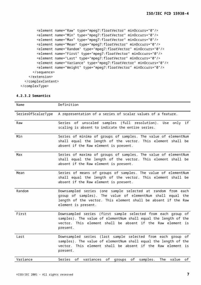
SeriesOfScalarType A representation of a series of scalar values of a feature.

Raw Series of unscaled samples (full resolution). Use only if scaling is absent to indicate the entire series.

Min Series of minima of groups of samples. The value of elementNum shall equal the length of the vector. This element shall be absent if the Raw element is present.

Max Series of maxima of groups of samples. The value of elementNum shall equal the length of the vector. This element shall be absent if the Raw element is present.

Mean Series of means of groups of samples. The value of elementNum shall equal the length of the vector. This element shall be absent if the Raw element is present.

Random Downsampled series (one sample selected at random from each group of samples). The value of elementNum shall equal the length of the vector. This element shall be absent if the Raw element is present.

First Downsampled series (first sample selected from each group of samples). The value of elementNum shall equal the length of the vector. This element shall be absent if the Raw element is present.

Last Downsampled series (last sample selected from each group of samples). The value of elementNum shall equal the length of the vector. This element shall be absent if the Raw element is present.

Variance Series of variances of groups of samples. The value of elementNum shall equal the length of the vector. This element shall be absent if the Raw element is present. Mean must be present in order for Variance to be present.

Weight Optional series of weights. Contrary to other fields, these do not represent values of the descriptor itself, but rather auxiliary weights to control scaling (see below). The value of elementNum shall equal the length of the vector.

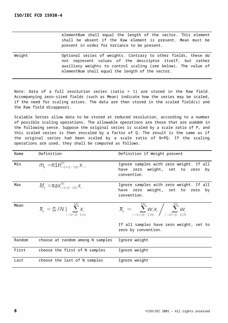
Note: Data of a full resolution series (ratio = 1) are stored in the Raw field. Accompanying zero-sized fields (such as Mean) indicate how the series may be scaled, if the need for scaling arises. The data are then stored in the scaled field(s) and the Raw field disappears.

Scalable Series allow data to be stored at reduced resolution, according to a number of possible scaling operations. The allowable operations are those that are scalable in the following sense. Suppose the original series is scaled by a scale ratio of P, and this scaled series is then rescaled by a factor of Q. The result is the same as if the original series had been scaled by a scale ratio of N=PQ. If the scaling operations are used, they shall be computed as follows.

Name Definition Definition if Weight present

Min Ignore samples with zero weight. If all have zero weight, set to zero by convention.

Max Ignore samples with zero weight. If all have zero weight, set to zero by convention.


ISO/IEC FCD 15938-4

Mean

If all samples have zero weight, set to zero by convention.

Random choose at random among N samples Ignore weight

First choose the first of N samples Ignore weight

Last choose the last of N samples Ignore weight

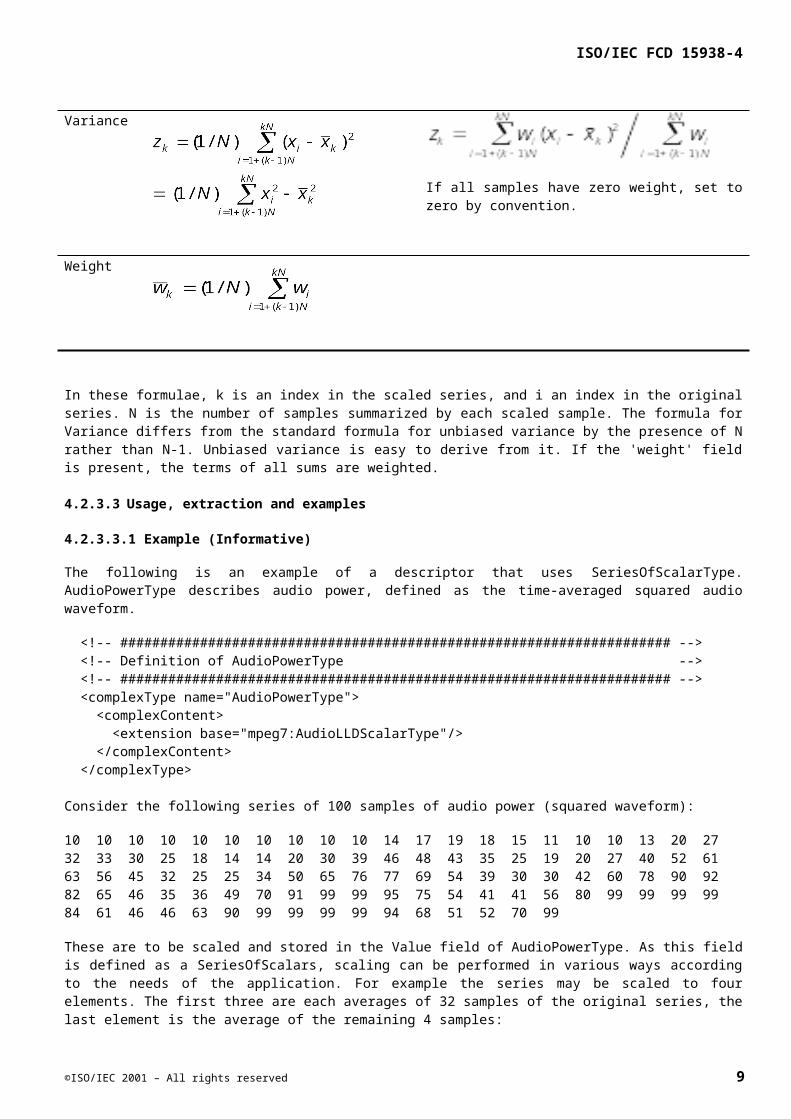
Variance


Weight

In these formulae, k is an index in the scaled series, and i an index in the original series. N is the number of samples summarized by each scaled sample. The formula for Variance differs from the standard formula for unbiased variance by the presence of N rather than N-1. Unbiased variance is easy to derive from it. If the 'weight' field is present, the terms of all sums are weighted.

4.2.3.3 Usage, extraction and examples

4.2.3.3.1 Example (Informative)

The following is an example of a descriptor that uses SeriesOfScalarType. AudioPowerType describes audio power, defined as the time-averaged squared audio waveform.

   <complexType name="AudioPowerType"> <complexContent> <extension base="mpeg7:AudioLLDScalarType"/> </complexContent> </complexType>

Consider the following series of 100 samples of audio power (squared waveform):

10 10 10 10 10 10 10 10 10 10 14 17 19 18 15 11 10 10 13 20 27 32 33 30 25 18 14 14 20 30 39 46 48 43 35 25 19 20 27 40 52 61 63 56 45 32 25 25 34 50 65 76 77 69 54 39 30 30 42 60 78 90 92 82 65 46 35 36 49 70 91 99 99 95 75 54 41 41 56 80 99 99 99 99 84 61 46 46 63 90 99 99 99 99 94 68 51 52 70 99


ISO/IEC FCD 15938-4

These are to be scaled and stored in the Value field of AudioPowerType. As this field is defined as a SeriesOfScalars, scaling can be performed in various ways according to the needs of the application. For example the series may be scaled to four elements. The first three are each averages of 32 samples of the original series, the last element is the average of the remaining 4 samples:

<Value totalSampleNum="100"> <Scaling ratio="32" elementNum="4"/> <Mean> 17.96 49.50 74.25 68 </Mean> </Value>

The data may also be stored at full resolution, with empty Mean and Variance fields that indicate how they may be scaled (if the need arises):

<Value totalSampleNum="100"> <Raw> 10 10 10 10 10 10 10 10 10 10 14 17 19 18 15 11 10 10 13 20 27 32 33 30 25 18 14 14 20 30 39 46 48 43 35 25 19 20 27 40 52 61 63 56 45 32 25 25 34 50 65 76 77 69 54 39 30 30 42 60 78 90 92 82 65 46 35 36 49 70 91 99 99 95 75 54 41 41 56 80 99 99 99 99 84 61 46 46 63 90 99 99 99 99 94 68 51 52 70 99 </Raw> <Mean/> <Variance/> </Value>

In the following example the same series is scaled to seven elements. The first and last are means of 50 and 45 samples respectively. The other 5 are individual samples that describe a restricted portion of the series at full resolution:

<Value totalSampleNum="100"> <Scaling ratio="50" elementNum="1"/> <Scaling ratio="1" elementNum="5"/> <Scaling ratio="45" elementNum="1"/> <Mean> 25.50 65 76 77 69 54 70.91 </Mean> </Value>

The same series may be summarized by four minima and maxima (the first three over 32 samples, the last over the remaining 4 samples):

<Value totalSampleNum="100"> <Scaling ratio="32" elementNum="4"/> <Min> 10 19 35 51 </Min> <Max> 46 92 99 99 </Max> </Value>

Suppose that associated with the above series is a series of "weights" that indicate which values are reliable and which are not. This makes sense if the values are fundamental frequencies produced by a pitch extractor:

0 0 0 0 0 0 0 0 0 0 1 1 1 1 1 1 0 0 1 1 1 1 1 1 1 1 1 1 1 1 1 1 1 1 1 1 1 1 1 1 1 1 1 1 1 1 1 1 1 1 1 1 1 1 1 1 1 1 1 1 1 1 1 1 1 1 1 1 1 1 1 0 0 1 1 1 1 1 1 1 0 0 0 0 1 1 1 1 1 1 0 0 0 0 1 1 1 1 1 0

Zero-weight values are de-emphasized in mean or variance calculations, and ignored in min and max calculations. The weights themselves are also stored to allow further scaling. Note that values of Mean, Min and Max, are not the same as in the previous unweighted examples:

<Value totalSampleNum="100"> <Scaling ratio="32" elementNum="4"/> <Min> 11 19 35 51 </Min> <Max> 46 92 95 70 </Max> <Mean> 22.75 49.50 63.00 57.67 </Mean>


ISO/IEC FCD 15938-4

<Variance> 87.7 432.3 369.5 76.22 </Variance> <Weight> 0.63 1.00 0.69 0.75 </Weight> </Value>

The following example illustrates a descriptor of type AudioPowerType attached to an audio segment. Note that the power descriptor contains data at two different resolutions:

<AudioSegment idref="111">  <AudioPower> <HopSize timeunit="PT1N44000F">1</HopSize>  <Value totalSampleNum="896"> <Scaling ratio="128" elementNum="6"/> <Mean> 0.96 1.2 0.43 0.7 0.2 0.97 0.15 </Mean> </Value> <Value totalSampleNum="896"> <Scaling ratio="896" elementNum="1"/> <Min>0.1</Min> <Max>1.3</Max> </Value> </AudioPower> </AudioSegment>

Note: AudioPower contains a field (HopSize, inherited from AudioSampledType) that specifies the period at which the descriptor was calculated. In the case of AudioPower this period is one sample at the waveform sampling rate. For other descriptors (for example FundamentalFrequency or SpectrumCentroid) the period is likely to be larger. Together, HopSize and Scaling define the periodicity of the scaled series.

4.2.4 SeriesOfScalarBinaryType

Use this type to instantiate a series of scalars with a uniform power-of-two Ratio. The restriction to a power-of-two ratio eases the comparison of series with different Ratios. It also allows an additional scaling operation to be defined (scalewise variance), and allows the data to be coded in "rootFirst" format, described below. Considering these computational properties of power-of-two scale ratios, the SeriesOfScalarBinaryType is the most useful of the ScalableSeries family.

4.2.4.1 Syntax

   <complexType name="SeriesOfScalarBinaryType"> <complexContent> <extension base="mpeg7:SeriesOfScalarType"> <sequence> <element name="VarianceScalewise" type="mpeg7:FloatMatrixType" minOccurs="0"/> </sequence> <attribute name="rootFirst" type="boolean" use="default" value="false"/> </extension> </complexContent> </complexType>

4.2.4.2 Semantics

Name Definition


ISO/IEC FCD 15938-4

SeriesOfScalarBinaryType A representation of a series of scalar values scaled by a power of two factor.

VarianceScalewise Optional array of arrays of scalewise variance coefficients. Scalewise variance is a decomposition of the variance into a series of coefficients, each of which describes the variability at a particular scale. There are log2(ratio) such coefficients. See definition below. Number of rows must equal 'NumElements', number of columns must equal the number of coefficients of the scalewise variance.

rootFirst Optional flag. If true, the series are recorded in "root-first" format. This format is defined below. In brief: the recorded series starts with the grand mean of the original series, and the subsequent values provide a progressively refined description from which the entire series can be reconstructed.


4.2.4.3.1 Root First format

Root first format is defined only for SeriesOfScalarBinaryType (uniform sampling with power-of-two ratio). Root first format is a way of rearranging the coefficients so that they represent the original series in a "coarse-first, fine-last" fashion. Based on the previous binary mean tree, the coefficients of yk the root first series are calculated as:

where is the mean (see the formula in section 4.2.3.2) of the tth group of 2s elements of the vector, and

m is log2 of the number of elements in the vector (rounded up).

The binary mean tree (and therefore the original series) can be reconstructed from this series:

The first coefficient is the grand mean. The second is the difference between the means of the first and second half of the series, from which these two means can be calculated, etc. rootFirst format may be useful to transmit a description over a slow network, for example to display a progressively-refined image of the descriptor.

Root First format is defined only for the 'mean' field. If 'rootFirst' is true, only the 'mean' field is allowed.

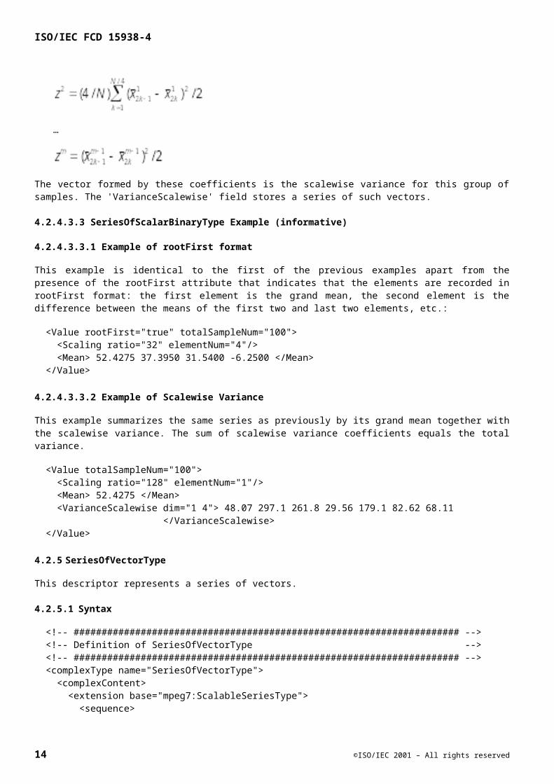
4.2.4.3.2 Scalewise Variance

Scalewise variance is a decomposition of the variance into a vector of coefficients that describe variability at different scales. The sum of these coefficients equals the variance. To calculate the scalewise variance of a set of N=2^m samples, first recursively form a binary tree of means:


ISO/IEC FCD 15938-4

…

Then calculate the coefficients:

…

The vector formed by these coefficients is the scalewise variance for this group of samples. The 'VarianceScalewise' field stores a series of such vectors.

4.2.4.3.3 SeriesOfScalarBinaryType Example (informative)

4.2.4.3.3.1 Example of rootFirst format

This example is identical to the first of the previous examples apart from the presence of the rootFirst attribute that indicates that the elements are recorded in rootFirst format: the first element is the grand mean, the second element is the difference between the means of the first two and last two elements, etc.:

<Value rootFirst="true" totalSampleNum="100"> <Scaling ratio="32" elementNum="4"/> <Mean> 52.4275 37.3950 31.5400 -6.2500 </Mean> </Value>

4.2.4.3.3.2 Example of Scalewise Variance

This example summarizes the same series as previously by its grand mean together with the scalewise variance. The sum of scalewise variance coefficients equals the total variance.

<Value totalSampleNum="100"> <Scaling ratio="128" elementNum="1"/> <Mean> 52.4275 </Mean> <VarianceScalewise dim="1 4"> 48.07 297.1 261.8 29.56 179.1 82.62 68.11 </VarianceScalewise> </Value>

4.2.5 SeriesOfVectorType

This descriptor represents a series of vectors.

4.2.5.1 Syntax

   <complexType name="SeriesOfVectorType"> <complexContent>


ISO/IEC FCD 15938-4

<extension base="mpeg7:ScalableSeriesType"> <sequence> <element name="Raw" type="mpeg7:FloatMatrixType" minOccurs="0"/> <element name="Min" type="mpeg7:FloatMatrixType" minOccurs="0"/> <element name="Max" type="mpeg7:FloatMatrixType" minOccurs="0"/> <element name="Mean" type="mpeg7:FloatMatrixType" minOccurs="0"/> <element name="Random" type="mpeg7:FloatMatrixType" minOccurs="0"/> <element name="First" type="mpeg7:FloatMatrixType" minOccurs="0"/> <element name="Last" type="mpeg7:FloatMatrixType" minOccurs="0"/> <element name="Variance" type="mpeg7:FloatMatrixType" minOccurs="0"/> <element name="Covariance" type="mpeg7:FloatMatrixType" minOccurs="0"/> <element name="VarianceSummed" type="mpeg7:floatVector" minOccurs="0"/> <element name="MaxSqDist" type="mpeg7:floatVector" minOccurs="0"/> <element name="Weight" type="mpeg7:floatVector" minOccurs="0"/> </sequence> <attribute name="vectorSize" type="positiveInteger" use="default" value="1"/> </extension> </complexContent> </complexType>

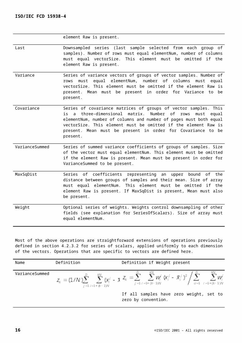
4.2.5.2 Semantics

Name Definition

SeriesOfVectorType An abstract type for scaled series of vectors.

Raw Series of unscaled samples (full resolution). Use only if Ratio=1 for the entire series.

Min Series of minima of groups of samples. Number of rows must equal elementNum, number of columns must equal vectorSize. This element must be omitted if the element Raw is present.

Max Series of maxima of groups of samples. Number of rows must equal elementNum,, number of columns must equal vectorSize. This element must be omitted if the element Raw is present.

Mean Series of means of groups of samples. Number of rows must equal elementNum, number of columns must equal vectorSize. This element must be omitted if the element Raw is present.

Random Downsampled series (one sample selected at random from each group of samples). Number of rows must equal elementNum, number of columns must equal vectorSize. This element must be omitted if the element Raw is present.

First Downsampled series (first sample selected from each group of samples). Number of rows must equal elementNum, number of columns must equal vectorSize. This element must be omitted if the element Raw is present.

Last Downsampled series (last sample selected from each group of samples). Number of rows must equal elementNum, number of columns must equal vectorSize. This element must be omitted if the element Raw is present.

Variance Series of variance vectors of groups of vector samples. Number of rows must equal elementNum, number of columns must equal vectorSize. This element must be


ISO/IEC FCD 15938-4

omitted if the element Raw is present. Mean must be present in order for Variance to be present.

Covariance Series of covariance matrices of groups of vector samples. This is a three-dimensional matrix. Number of rows must equal elementNum, number of columns and number of pages must both equal vectorSize. This element must be omitted if the element Raw is present. Mean must be present in order for Covariance to be present.

VarianceSummed Series of summed variance coefficients of groups of samples. Size of the vector must equal elementNum. This element must be omitted if the element Raw is present. Mean must be present in order for VarianceSummed to be present.

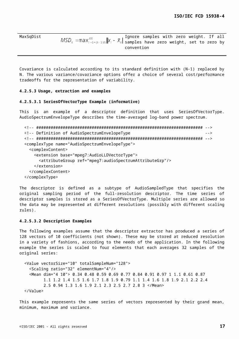
MaxSqDist Series of coefficients representing an upper bound of the distance between groups of samples and their mean. Size of array must equal elementNum. This element must be omitted if the element Raw is present. If MaxSqDist is present, Mean must also be present.

Weight Optional series of weights. Weights control downsampling of other fields (see explanation for SeriesOfScalars). Size of array must equal elementNum.

Most of the above operations are straightforward extensions of operations previously defined in section 4.2.3.2 for series of scalars, applied uniformly to each dimension of the vectors. Operations that are specific to vectors are defined here.

Name Definition Definition if Weight present

VarianceSummed


MaxSqDist Ignore samples with zero weight. If all samples have zero weight, set to zero by convention

Covariance is calculated according to its standard definition with (N-1) replaced by N. The various variance/covariance options offer a choice of several cost/performance tradeoffs for the representation of variability.


4.2.5.3.1 SeriesOfVectorType Example (informative)

This is an example of a descriptor definition that uses SeriesOfVectorType. AudioSpectrumEnvelopeType describes the time-averaged log-band power spectrum.

   <complexType name="AudioSpectrumEnvelopeType"> <complexContent>


ISO/IEC FCD 15938-4

<extension base="mpeg7:AudioLLDVectorType"> <attributeGroup ref="mpeg7:audioSpectrumAttributeGrp"/> </extension> </complexContent> </complexType>

The descriptor is defined as a subtype of AudioSampledType that specifies the original sampling period of the full-resolution descriptor. The time series of descriptor samples is stored as a SeriesOfVectorType. Multiple series are allowed so the data may be represented at different resolutions (possibly with different scaling rules).

4.2.5.3.2 Description Examples

The following examples assume that the descriptor extractor has produced a series of 128 vectors of 10 coefficients (not shown). These may be stored at reduced resolution in a variety of fashions, according to the needs of the application. In the following example the series is scaled to four elements that each averages 32 samples of the original series:

<Value vectorSize="10" totalSampleNum="128"> <Scaling ratio="32" elementNum="4"/> <Mean dim="4 10"> 0.34 0.48 0.59 0.69 0.77 0.84 0.91 0.97 1 1.1 0.61 0.87 1.1 1.2 1.4 1.5 1.6 1.7 1.8 1.9 0.79 1.1 1.4 1.6 1.8 1.9 2.1 2.2 2.4 2.5 0.94 1.3 1.6 1.9 2.1 2.3 2.5 2.7 2.8 3 </Mean> </Value>

This example represents the same series of vectors represented by their grand mean, minimum, maximum and variance.

<Value vectorSize="10" totalSampleNum="128"> <Scaling ratio="128" elementNum="1"/> <Min dim="1 10"> 0.1 0.14 0.17 0.2 0.22 0.2 0.26 0.2 0.3 0.32 </Min> <Max dim="1 10"> 1 1.4 1.7 2 2.2 2.4 2.6 2.8 3 3.2 </Max> <Mean dim="1 10"> 0.67 0.95 1.2 1.3 1.5 1.6 1.8 1.9 2 2.1 </Mean> <Variance dim="1 10"> 0.05 0.11 0.16 0.2 0.27 0.3 0.3 0.4 0.4 0.54 </Variance> </Value>

This example summarizes the same series vectors represented by their covariance matrix.

<Value vectorSize="10" totalSampleNum="128"> <Scaling ratio="128" elementNum="1"/> <Mean dim="1 10"> 0.67 0.95 1.2 1.3 1.5 1.6 1.8 1.9 2 2.1 </Mean> <Covariance dim="1 10 10"> 0.054 0.077 0.094 0.11 0.12 0.13 0.14 0.15 0.16 0.17 0.077 0.11 0.13 0.15 0.17 0.19 0.2 0.22 0.23 0.24 0.094 0.13 0.16 0.19 0.21 0.23 0.25 0.27 0.28 0.3 0.11 0.15 0.19 0.22 0.24 0.27 0.29 0.31 0.32 0.34 0.12 0.17 0.21 0.24 0.27 0.3 0.32 0.34 0.36 0.38 0.13 0.19 0.23 0.27 0.3 0.32 0.35 0.38 0.4 0.42 0.14 0.2 0.25 0.29 0.32 0.35 0.38 0.41 0.43 0.45 0.15 0.22 0.27 0.31 0.34 0.38 0.41 0.43 0.46 0.48 0.16 0.23 0.28 0.32 0.36 0.4 0.43 0.46 0.49 0.51 0.17 0.24 0.3 0.34 0.38 0.42 0.45 0.48 0.51 0.54 </Covariance> </Value>

This example represents the same series vectors represented by a series of 4 VarianceSummed coefficients, each of which represents the variance (summed over vector coefficients) calculated separately over groups of 32 samples.

<Value vectorSize="10" totalSampleNum="128"> <Scaling ratio="32" elementNum="4"/> <VarianceSummed> 0.70 0.19 0.11 0.082 </VarianceSummed> </Value>


ISO/IEC FCD 15938-4

4.2.6 SeriesOfVectorBinaryType

Use this type to instantiate a series of vectors with a uniform power-of-two Ratio. The restriction to a power-of-two ratio eases the comparison of series with different Ratios. It also allows an additional scaling operation to be defined (scalewise variance), and allows the data to be coded in "rootFirst" format, described above in section 4.2.4.3.1. The use of power-of-two scale ratios is recommended.

4.2.6.1 Syntax

   <complexType name="SeriesOfVectorBinaryType"> <complexContent> <extension base="mpeg7:SeriesOfVectorType"> <sequence> <element name="VarianceScalewise" type="mpeg7:FloatMatrixType" minOccurs="0"/> </sequence> <attribute name="rootFirst" type="boolean" use="default" value="false"/> </extension> </complexContent> </complexType>

4.2.6.2 Semantics

Name Definition

SeriesOfVectorBinaryType A representation of a reduced-resolution series of vector samples with a power-of-two Ratio.

VarianceScalewise Array of arrays of scalewise summed-variance coefficients. Scalewise variance is a decomposition of the variance into a series of coefficients, each of which describes the variability at a particular scale. Number of rows must equal elementNum, number of columns must equal the number of coefficients of the scalewise variance.

rootFirst If true, the series are recorded in “root-first” format. Each row is reordered in the same way elements are reordered in SeriesOfScalarBinaryType, and individual elements in each row are mean-difference encoded in the way outlined in SeriesOfScalarBinaryType.

4.2.7 Examples of Applications of Scalable Series (informative)

4.2.7.1 Example of continual rescaling of series

The application is remote monitoring of parameters (weather, seismic, plant process, etc.). Data from the sensors are recorded at full resolution and stored in a circular buffer, and simultaneously a low-resolution scaled version is sent over the network (as an MPEG-7 stream). At regular intervals the circular buffer is transferred to disk (as an MPEG-7 file). To avoid running out of disk space, the full-resolution files are regularly processed to obtain scaled files (also in MPEG-7 format). The oldest scaled files are themselves rescaled according to a schedule that ensures that disc space never runs out. This record contains a complete history of the parameter, with temporal resolution that is reduced for older data. A set of statistics such as extrema (min, max), mean, variance, etc. give useful information about the data that were discarded in the scaling process.


ISO/IEC FCD 15938-4

The Scalable Series support:

a) the low-resolution representation for streaming over a low-bandwidth network

b) the storage at full- or reduced-resolution

c) the arbitrary scaling and rescaling to fit within a finite storage volume

d) statistics to characterize aspects of the data that may have been lost due to scaling: extrema, mean, variability.

4.2.8 Examples of search algorithms based on scalable series

These examples illustrate how scalable series may be used for efficient search. The purpose is not to define algorithms rigorously, but rather to give ideas on how search applications might be addressed. ScalableSeries allow storage of useful statistics to support search, comparison and clustering. The reduced-resolution data serve either as a surrogate of the original data if it is unavailable, or as a short-cut to the original data if it is available but expensive to access. They make search possible in the first case, and fast in the second.

As an example, consider a large database of audio. The task is to determine whether a given snippet of audio belongs to the database based on spectral similarity. A straightforward procedure is to scan the database, calculate spectra for each frame and compare them to spectra of the snippet. For an even moderately-sized database this is likely to be too expensive for two reasons: the high cost of data access/spectrum calculation, and the inefficiency of linear search. To reduce the former cost, the spectra may be precomputed, but this requires large amounts of storage to keep the spectra. Also it does not address the second cost, that of linear search through the spectra. ScalableSeries address both costs: they allow storage in a cheap low-resolution format that supports efficient search. Typically a feature may be extracted as a series of 'N' samples. This is scaled to 'm' elements that each summarizes a group of 'n' samples ( ). Search occurs in two steps: first among the 'm' elements for the 'q' best candidates, and then among the 'n' samples of each candidate. The ( )-step search is thus replaced by a (

)-step search. This is fast if q<<m, that is, if groups are labeled with information that allows the algorithm to decide whether they are good candidates. That is the purpose of the statistics afforded by ScalableSeries.

For the following section, it is useful to think of the scaled series as being one layer of a tree. The leaves are the samples of the original full-resolution series, the root is a single summary value obtained by scaling the series by a scale ratio equal to its number of samples. To be specific we can suppose that it is a binary tree (n-ary trees may be more effective in practice). Starting from the series of 'N' samples, a (2N-1)-node balanced binary tree is formed by repeatedly applying the scaling operation. Search then proceeds from the root, with a cost that may be as small as O(log2(N)). In practice, the search algorithms may use only part of this tree, but to keep things simple they are described as using the full tree. The following algorithms refer to this tree.

4.2.8.1 Search and comparison using Min and Max

The 'Min' and 'Max' fields of a SeriesOfScalars store series of 'min' and 'max' of groups of samples. 'Min' and 'Max' fields of SeriesOfVector store similar information for groups of vectors in a series.

Suppose that a binary tree has been constructed based on samples of a series of scalars, each node containing a min-max pair summarizing the group of samples that it spans. The task is to determine whether a sample 'x' appears within the series.

Algorithm: Starting from the root, at each node test whether 'x' is between 'min' and 'max'. If it is, recurse on both child nodes. If it is not, prune the subtree (ignore all child nodes).

Search is fast if a large proportion of the tree is pruned. In the case that a single layer of 'm' nodes is available, the test is performed on each, and those for which it fails are discarded. The search then proceeds by accessing (or recalculating) the data spanned by the successful nodes. Search is fast if these are few.


ISO/IEC FCD 15938-4

Suppose that min-max binary trees have been constructed for two series (segments) of scalars 'A' and 'B'. The task is to determine whether segment A is included within segment B. The algorithm is based on the fact that the min and max of an interval are intermediate between the min and max of any interval that includes it.

Algorithm: In a first step, tree B is processed by merging adjacent nodes of each layer. For layer j, node k is merged with node k+1:

This step is necessary because intervals of groups of samples subsumed by nodes of trees A and B might not be aligned. The second step is to compare the min-max pair of the root of A to nodes of B, starting at the root. This process stops at the depth where each node of B spans an interval just large enough to contain the interval spanned by A. Nodes for which this test fails are pruned. The third step consists of comparing A and B layer by layer. For each layer of A, take the first node of and compare it to successive nodes of the corresponding layer of B, pruning those for which this test fails. If the test succeeds for a certain node of B, compare the next nodes of A to the next nodes of B. If this test succeeds, the comparison may then proceed to the next layer. If it fails, and if all nodes of B have been tested, the algorithm declares that A is not included in B.

Search is fast if the trees can be pruned rapidly. It is much faster than with other approaches such as sample-to-sample comparison or cross-correlation. The algorithm may be made yet faster (but more complex) by checking that candidate nodes of B are in included in A. It may be extended to test whether files A and B have a common intersection. The algorithm may be usefully applied to find duplicates among files, or in an editing application to identify common waveform segments.

4.2.8.2 Search and comparison using Mean and Variance

As a rough approximation, the distribution of scalar samples within a group may be modeled by a Gaussian distribution characterized by its mean and variance. For multidimensional data the covariance matrix is used in place of variance, but it may be approximated by its diagonal terms (vector of per-dimension variance terms) which can themselves be summarized by their sum. The covariance matrix characterizes an ellipsoidal approximation to the distribution, the variance vector characterizes the same with axes aligned to the dimensions, and their sum characterizes a spherical approximation. Whatever the quality of the approximation, it may be used to infer the probability that a particular search token belongs to the distribution. This allows effective search.

As for search based on extrema (min-max, or maximum squared distance from mean), efficiency results from pruning the search tree (or ordering it to start the search in the most likely place). Pruning was deterministic for extrema, it is probabilistic in the case of mean and variance. For example, the search may decide to prune nodes that are distant by more than two or three standard deviations from the search token.

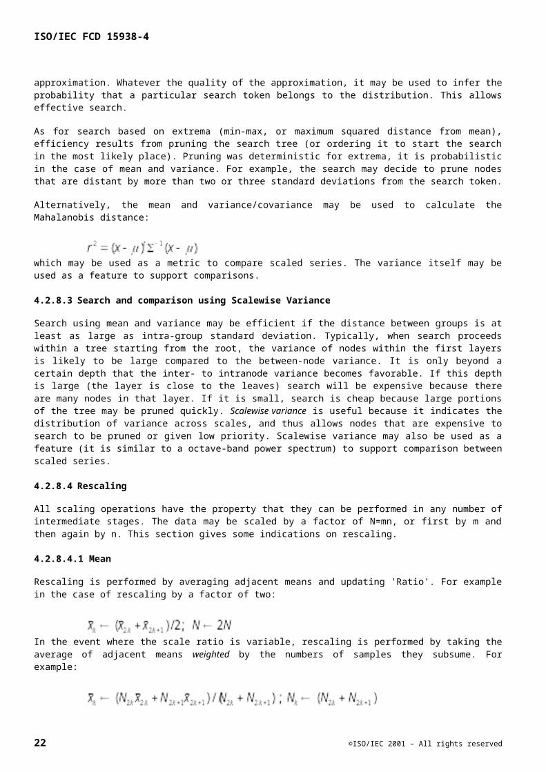
Alternatively, the mean and variance/covariance may be used to calculate the Mahalanobis distance:

which may be used as a metric to compare scaled series. The variance itself may be used as a feature to support comparisons.

4.2.8.3 Search and comparison using Scalewise Variance

Search using mean and variance may be efficient if the distance between groups is at least as large as intra-group standard deviation. Typically, when search proceeds within a tree starting from the root, the variance of nodes within the first layers is likely to be large compared to the between-node variance. It is only beyond a certain depth that the inter- to intranode variance becomes favorable. If this depth is large (the layer is close to the leaves) search will be expensive because there are many nodes in that layer. If it is small, search is cheap because large portions of the tree may be pruned quickly. Scalewise variance is useful because it indicates the distribution of variance across scales, and thus allows nodes that are expensive to search to be pruned or given low priority. Scalewise variance may also be used as a feature (it is similar to a octave-band power spectrum) to support comparison between scaled series.


ISO/IEC FCD 15938-4

4.2.8.4 Rescaling

All scaling operations have the property that they can be performed in any number of intermediate stages. The data may be scaled by a factor of N=mn, or first by m and then again by n. This section gives some indications on rescaling.

4.2.8.4.1 Mean

Rescaling is performed by averaging adjacent means and updating 'Ratio'. For example in the case of rescaling by a factor of two:

In the event where the scale ratio is variable, rescaling is performed by taking the average of adjacent means weighted by the numbers of samples they subsume. For example:

In the event where a Weight field is present, operations are weighted by this factor also.

4.2.8.4.2 Min, max

Rescaling is performed by taking the min (resp. max) of adjacent samples. For example in the case of rescaling by a factor of two:

In the event where a Weight field is present, samples with zero weight are ignored in the min (resp. max) operation. If all samples involved have zero weight, the result also has zero weight (it is set to zero by convention).

4.2.8.4.3 Variance

Rescaling is performed by taking the average of variances of adjacent samples, and adding the biased variance of the corresponding means. For example in the case of downsampling by a factor of two:

In the case that scale ratios are present, or a weight field is present, appropriate weights are used within these calculations. Scaling of variance requires the presence of the mean (if a SeriesOfScalars contains a 'Variance' field it must also contain a 'Mean' field).

4.2.8.4.4 Scalewise variance

Scaling involves two operations. First, adjacent scalewise variance coefficients are averaged:

Then, a new coefficient is derived from the means of layer m:

Scaling of scalewise variance requires the presence of the mean (if a SeriesOfScalars contains a VarianceScalewise field it must also contain a Mean field).


ISO/IEC FCD 15938-4

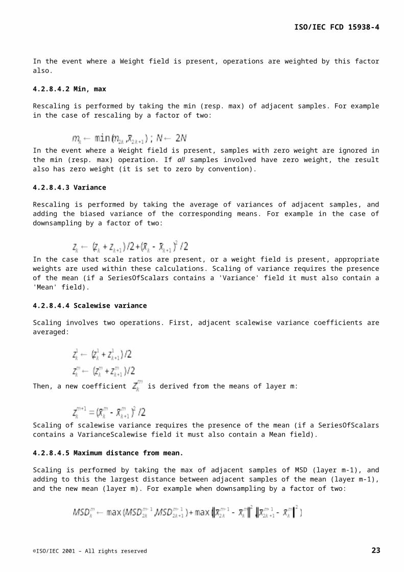
4.2.8.4.5 Maximum distance from mean.

Scaling is performed by taking the max of adjacent samples of MSD (layer m-1), and adding to this the largest distance between adjacent samples of the mean (layer m-1), and the new mean (layer m). For example when downsampling by a factor of two:


ISO/IEC FCD 15938-4

4.3 Low level Audio Descriptors

4.3.1 Introduction

Low-level Audio Descriptors (LLDs) consist of a collection of simple, low complexity descriptors that are designed to be used within the AudioSegment framework, see ISO-IEC 15938-5 (E). Whilst being useful in themselves, they also provide examples of a design framework for future extension of the audio descriptors and description schemes.

All low-level audio descriptors are defined as subtypes of either AudioLLDScalarType or AudioLLDVectorType. There are two description strategies using these data types; single-valued summary and sampled series segment description. These two description strategies are made available for the two data types, scalar/SeriesOfScalarType and vectorType/SeriesOfVectorType, and are implemented as a choice in DDL.

When using summary descriptions (containing a single scalar or vector) there are no normative methods for calculating the single-valued summarization. However, when using series-based descriptions, the summarization values shall be calculated using the scaling methods provided by the SeriesOfScalarType and SeriesOfVectorType descriptors, such as the min, max and mean operators.

4.3.2 AudioLLDScalarType

4.3.2.1 Syntax

   <complexType name="AudioLLDScalarType" abstract="true"> <complexContent> <extension base="mpeg7:AudioDType"> <choice> <element name="Scalar" type="float"/> <element name="SeriesOfScalar"> <complexType> <complexContent> <extension base="mpeg7:SeriesOfScalarType"> <attribute name="hopSize" type="mpeg7:mediaDurationType" use="default" value="10F1000"/> </extension> </complexContent> </complexType> </element> </choice> </extension> </complexContent> </complexType>

4.3.2.2 Semantics

Name Definition

AudioLLDScalarType Abstract definition inherited by all scalar datatype audio descriptors.

Scalar Value of the descriptor

SeriesOfScalar Scalar values for sampled-series description of an audio segment. Use of this scalable


ISO/IEC FCD 15938-4

Name Definition

series datatype promotes compatibility between sampled descriptions.

hopSize Time interval between data samples for series description. The default value is “10F1000” which is 10 milliseconds.

Values other than the default shall be integer multiples of 10 milliseconds. This will ensure compatibility of descriptors sampled at different rates.

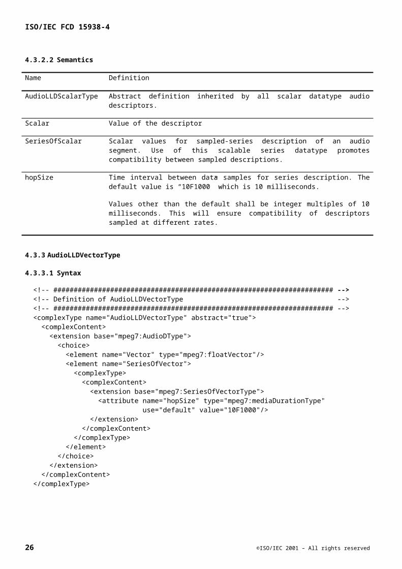
4.3.3 AudioLLDVectorType

4.3.3.1 Syntax

   <complexType name="AudioLLDVectorType" abstract="true"> <complexContent> <extension base="mpeg7:AudioDType"> <choice> <element name="Vector" type="mpeg7:floatVector"/> <element name="SeriesOfVector"> <complexType> <complexContent> <extension base="mpeg7:SeriesOfVectorType"> <attribute name="hopSize" type="mpeg7:mediaDurationType" use="default" value="10F1000"/> </extension> </complexContent> </complexType> </element> </choice> </extension> </complexContent> </complexType>

4.3.3.2 Semantics

Name Definition

AudioLLDVectorType Abstract definition inherited by all vector datatype audio descriptors.

Vector Vector value of descriptor

SeriesOfVector Vector values for sampled-series description of an audio segment. Use of this scalable series datatype promotes compatibility between sampled descriptions.

hopSize Time interval between data samples for series description. The default value is “10F1000” which is 10 milliseconds.

Values other than the default shall be integer multiples of 10 milliseconds. This will ensure compatibility of descriptors sampled at different rates.


ISO/IEC FCD 15938-4

4.3.3.3 Usage and Extraction

Audio descriptors that calculated at regular intervals (sample period or frame period) shall use the hopSize field to specify the extraction period. In all cases, the hopSize shall be a positive integer multiple of the default 10 millisecond sampling period. Note that downsampling by means of the scalable series does not change the specified hopSize but instead specifies the downsampling scale ratio to be used together with the hopSize.

AudioLLDScalarType and AudioLLDVectorType are both abstract and therefore never instantiated.

4.3.4 AudioWaveformType

AudioWaveFormType describes the audio waveform envelope, typically for display purposes.

4.3.4.1 Syntax

   <complexType name="AudioWaveformType"> <complexContent> <extension base="mpeg7:AudioLLDScalarType"> <attribute name="minRange" type="float"/> <attribute name="maxRange" type="float"/> </extension> </complexContent> </complexType>

4.3.4.2 Semantics

Name Definition

AudioWaveformType Description of the waveform of the audio signal.

minRange Lower limit of audio signal amplitude

maxRange Upper limit of audio signal amplitude

4.3.4.3 Usage and extraction

4.3.4.3.1 Purpose

AudioWaveformType allows economical display of an audio waveform. For example, a sound editing application program can display a summary of an entire audio file immediately without processing the audio data and data may be displayed and edited over a network, etc. Whatever the number of samples, the waveform may be displayed using a small set of values that represent extrema (min and max) of frames of samples. Min and max are stored as scalable time series within the AudioWaveformType. They may also used for fast comparison between waveforms.

4.3.4.3.2 To create a description

a) Instantiate an AudioWaveformType with hopSize set to 10ms.

b) Determine the appropriate ScaleRatio based on the required resolution.


ISO/IEC FCD 15938-4

c) If the scale ratio is equal to 1, instantiate a SeriesOfScalarType with a Raw field and store waveform samples directly. Instantiate also empty Min and Max fields to allow rescaling. If the scale ratio differs from 1, instantiate Min and Max fields and fill them with scaled samples. The scale ratio may be variable over the series.

4.3.4.3.3 To use a description for display

d) Read the arrays of min and max values from the AudioWaveformType.

e) For each min/max pair, draw a vertical line from min to max.

f) Label axes using the scaling information.

4.3.5 AudioSpectrumEnvelopeType

AudioSpectrumEnvelopeType describes the spectrum of the audio according to a logarithmic frequency scale. The attributes are defined as an attributeGroup as they are also used for the sound recognition tools.

4.3.5.1 Syntax

   <attributeGroup name="audioSpectrumAttributeGrp"> <annotation> <documentation>Edge values are in Hertz</documentation> </annotation> <attribute name="loEdge" type="float" use="default" value="62.5"/> <attribute name="hiEdge" type="float" use="default" value="16000"/> <attribute name="resolution"> <simpleType> <restriction base="string"> <enumeration value="1/16 octave"/> <enumeration value="1/8 octave"/> <enumeration value="1/4 octave"/> <enumeration value="1/2 octave"/> <enumeration value="1 octave"/> <enumeration value="2 octave"/> <enumeration value="4 octave"/> <enumeration value="8 octave"/> </restriction> </simpleType> </attribute> </attributeGroup>

   <complexType name="AudioSpectrumEnvelopeType"> <complexContent> <extension base="mpeg7:AudioLLDVectorType"> <attributeGroup ref="mpeg7:audioSpectrumAttributeGrp"/> </extension> </complexContent> </complexType>


ISO/IEC FCD 15938-4

4.3.5.2 Semantics

Name Definition

AudioSpectrumEnvelopeType Description of the power spectrum of the audio signal. The spectrum consists of one coefficient representing power between 0Hz and loEdge, a series of coefficients representing power in logarithmically spaced bands between loEdge and hiEdge, and a coefficient representing power beyond hiEdge, in this order.

loEdge Lower edge of logarithmically-spaced frequency bands.

hiEdge Higher edge of logarithmically-spaced frequency bands.

resolution Frequency resolution of logarithmic spectrum (width of each spectrum band between loEdge and hiEdge).


4.3.5.3.1 Purpose

The AudioSpectrumEnvelopeType describes the short-term power spectrum of the audio waveform as a time series of spectra with a logarithmic frequency axis. It may be used to display a spectrogram, to synthesize a crude "auralization" of the data, or as a general-purpose descriptor for search and comparison.

4.3.5.3.2 Specification of the descriptor

In the interests of interoperability, the AudioSpectrumEnvelopeType is specified in detail. These specifications are normative and ensure that descriptions produced by different programs are either directly comparable, or else can easily be converted to comparable descriptions.

A logarithmic frequency axis is used to conciliate requirements of concision and descriptive power. Peripheral frequency analysis in the ear roughly follows a logarithmic axis

The power spectrum is used because of its scaling properties (the power spectrum over an interval is equal to the sum of power spectra over subintervals).

The AudioSpectrumEnvelopeType describes a frequency range between loEdge and hiEdge, which must be chosen in octave relation to 1kHz as described in the following equation, except for when the resolution is "8 octave": If is the resolution in octaves,

,

where (i.e., an integer).

For the case when resolution is "8 octave" the spectrum delivers a single coefficient representing within-band power, and two extra coefficients for below-band and above-band power. In this case the default values for loEdge and hiEdge should be used.

Default hiEdge is 16000Hz (corresponding to the upper limit of hearing). Default loEdge is 62.5 Hz (8 octaves below hiEdge). The range between loEdge and hiEdge is divided according to power-of-two ratios. The resolution is specified by resolution. In every case the spectrum contains two extra values, one representing the energy between 0Hz and loEdge, and the other energy between hiEdge and half the sampling rate (See


ISO/IEC FCD 15938-4

Figure 1). These values measure the "out-of-band" energy. Importantly, a high-resolution description is readily convertible to a low-resolution description.

62.5 1K 16000

1 coeff 8 coeffs 1 coeff

total power

within-bandbelow-band above-band

Figure 1 - Illustration of Audio Spectrum Envelope Bands

The analysis frame period shall be 10 ms, which is within the range of estimates for temporal acuity of the ear (8 to 13 ms) and is also the default analysis frame period for sampled audio descriptors.

4.3.5.3.3 Extraction

To extract the AudioSpectrumEnvelope the following method is recommended. The method involves a sliding window FFT analysis, with a resampling to logarithmic spaced bands.

The analysis frame period has been specified as 10ms however a sliding extraction window, 30ms in duration, is used with a Hamming window. 30ms is chosen to provide enough spectral resolution to roughly resolve the 62.5 Hz-wide first channel of an octave-band spectrum. The size of the FFT analysis window is the next-larger power-of-two number of samples. 30ms at 32kHz is 960 samples but the FFT would be performed on 1024 samples, 30ms at 44.1 KHz is 1323 samples but the FFT would be performed on 2048 samples with out-of-window samples set to 0.

Figure 2 - Weighting Method for linear - log conversionThe mapping between log scale and linear scale power spectrum coefficients is straightforward. If DF is the frequency spacing of the FFT (DF = sampling rate/FFT size), a coefficient more than DF/2 from a band edge is assigned to the band. A coefficient less than DF/2 from the edge is proportionally shared between bands, as illustrated in Figure 2. The sum of coefficients (total power) remains the same.

Due to the weighting method illustrated in Figure 2 it is important to select an appropriate loEdge at fine frequency resolutions. To be able to resolve the logarithmic bands there needs to be at least one FFT coefficient in each band. In some cases this means that the default loEdge is unsuitable. Table 1 indicates the minimum value that loEdge should be set to for some popular sampling frequencies.

The sum of all spectral coefficients is equal to the total power in the analysis window


ISO/IEC FCD 15938-4

Resolution Minimum loEdge(using DF = 31.25,FFT size 1024, SR = 32kHzFFT size 512, SR = 16kHz)

Minimum loEdge(using DF = 21.53,FFT size 2048, SR = 44.1kHz)

Minimum loEdge(using DF = 23.44,FFT size 2048, SR = 48kHz)

¼ 88.388 (62.5*20.5) 62.5 105.1 (62.5*23/4)1/8 324.21 (62.5*219/8) 162.1 (62.5*211/8) 192.78 (62.5*213/8)1/16 545.25 (62.5*225/8) 420.45 (62.5*211/4) 478.8 (62.5*247/16)

Table 1 Minimum loEdge for particular resolutions (exceeding default 62.5Hz)

The sum of all spectral coefficients is equal to the total power in the analysis window

4.3.5.4 To create a description

Instantiate AudioSpectrumEnvelopeType with hopSize set to the 10 ms frame period. Decide the requisite frequency resolution.

For each frame: window the audio data, calculate the FFT, calculate the power of each coefficient (squared magnitude), resample to a log scale using the above mapping.

4.3.6 AudioPowerType

AudioPowerType describes the temporally-smoothed instantaneous power (square of waveform values).

4.3.6.1 Syntax

   <complexType name="AudioPowerType"> <complexContent> <extension base="mpeg7:AudioLLDScalarType"/> </complexContent> </complexType>

4.3.6.2 Semantics

Name Definition

AudioPowerType Description of the power of the audio signal.



Instantaneous power is calculated by taking the square of waveform samples. These are averaged over groups of samples and stored in the 'Mean' field of a SeriesOfScalarType. Time interval between data samples shall be an integer multiple of 10 milliseconds. This will ensure compatibility of descriptors sampled at different rates.

4.3.6.3.2 Purpose

Instantaneous power is useful to measure of the amplitude of a signal as a function of time. In association with spectral centroid and spectral spread, it provides an economical description of the power spectrum, that can be compared for example with a log-frequency spectrum. Another possibility is to store instantaneous power at high


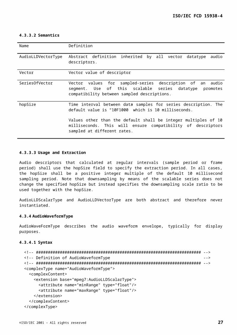
ISO/IEC FCD 15938-4

temporal resolution, in association with a high-resolution power spectrum at low resolution, to obtain a cheap representation of the power spectrum that combines both spectral and temporal resolution.

4.3.6.3.3 Motivation for the design

Instantaneous power is coherent with the power spectrum. A signal labeled with the former can meaningfully be compared to a signal labeled with the latter. Note however that temporal smoothing operations are not quite the same, so values may differ slightly for identical signals.

4.3.7 AudioSpectrumCentroidType

AudioSpectrumCentroidType describes the center of gravity of the log-frequency power spectrum. The SpectrumCentroid is defined as the power weighted log-frequency centroid.

4.3.7.1 Syntax

    <complexType name="AudioSpectrumCentroidType"> <complexContent> <extension base="mpeg7:AudioLLDScalarType"/> </complexContent> </complexType>

4.3.7.2 Semantics

Name Definition

AudioSpectrumCentroidType Description of the center of gravity of the log-frequency power spectrum.



To be coherent with other descriptors, in particular AudioSpectrumEnvelopeType, the spectrum centroid is defined as the center-of-gravity of a log-frequency power spectrum. This definition is adjusted to take into account the fact that a non-zero DC component creates a singularity, and eventual very-low frequency components (possibly spurious) have a disproportionate weight.

To extract the spectrum centroid:

a) Calculate the DFT of the waveform as for AudioSpectrumEnvelopeType: 30-ms segments of signal are excised at 10-ms intervals, a raised cosine window is applied, the window is zero-padded to the next power of two number of samples, and an FFT performed.

b) The power is calculated as the square magnitude of FFT coefficients.

c) Samples below 62.5 Hz are replaced by a single sample, with power equal to their sum and a nominal frequency of 31.25 Hz.

d) Frequencies of all samples are scaled to an octave scale anchored at 1 kHz, and the spectrum centroid is

calculated as: where is the power associated with frequency .


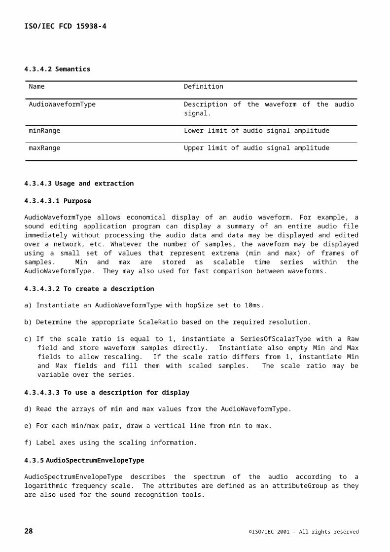
ISO/IEC FCD 15938-4

4.3.7.3.2 Purpose

Spectrum centroid is an economical description of the shape of the power spectrum. It indicates whether the power spectrum is dominated by low or high frequencies and, additionally, it is correlated with a major perceptual dimension of timbre; i.e.sharpness.


There are many different ways to design a spectrum centroid, according to the scale used for the values (amplitude, power, log power, cubic root power, etc.) and frequencies (linear or logarithmic scale) of spectrum coefficients. Perceptual weighting and masking can also be taken into account in more sophisticated measures. This particular design of AudioSpectrumCentroidType was chosen to be coherent with other descriptors, in particular AudioSpectrumEnvelopeType, so that a signal labeled with the former can reasonably be compared to a signal labeled with the latter.

The logarithmic frequency scale provides a reasonably close match to the distribution of auditory filters across the spectrum. It is likely that more sophisticated measures would be better predictors of psychophysical sharpness, at the expense of greater complexity and reduced coherence with other descriptors.

4.3.8 AudioSpectrumSpreadType

AudioSpectrumSpreadType describes the second moment of the log-frequency power spectrum.

4.3.8.1 Syntax

    <complexType name="AudioSpectrumSpreadType"> <complexContent> <extension base="mpeg7:AudioLLDScalarType"/> </complexContent> </complexType>

4.3.8.2 Semantics

Name Definition

AudioSpectrumSpreadType Description of the spread of the log-frequency power spectrum.



To be coherent with other descriptors, in particular AudioSpectrumEnvelopeType, the spectrum centroid is defined as the RMS deviation of the log-frequency power spectrum with respect to its center of gravity. Details are similar to AudioSpectrumCentroidType.

To extract the spectrum spread:

a) Calculate the power spectrum of the waveform and scale it to a log frequency scale, as for AudioSpectrumCentroidType. Samples below 62.5 Hz are grouped as before.

b) Calculate the spectrum centroid as defined previously.


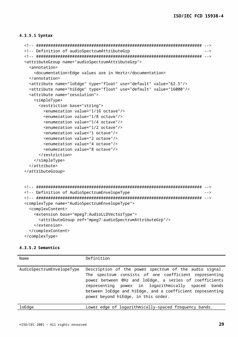
ISO/IEC FCD 15938-4

c) Calculate the spectrum spread as the RMS deviation with respect to the centroid, on an octave scale:

4.3.8.3.2 Purpose

Spectrum spread is an economical descriptor of the shape of the power spectrum that indicates whether it is concentrated in the vicinity of its centroid, or else spread out over the spectrum. It allows differentiating between tone-like and noise-like sounds.


As for the spectrum centroid, there are many different ways to design a spectrum spread measure. This definition follows the same criteria as AudioSpectrumCentroidType, with which it is coherent.

4.3.9 AudioSpectrumFlatnessType

AudioSpectrumFlatnessType describes the flatness properties of the spectrum of an audio signal within a given number of frequency bands.

4.3.9.1 Syntax

   <complexType name="AudioSpectrumFlatnessType"> <complexContent> <extension base="mpeg7:AudioLLDVectorType"> <attribute name="numBands" use="default" value="8"> <simpleType> <restriction base="string"> <enumeration value="4"/> <enumeration value="8"/> <enumeration value="16"/> </restriction> </simpleType> </attribute> </extension> </complexContent> </complexType>

4.3.9.2 Semantics

Name Definition

AudioSpectrumFlatnessType Description of the audio spectral flatness of the audio signal.

numBands Subdivision in number of bands (a default resolution of 8 bands is assumed)

4.3.9.3 Usage, extraction and examples (informative)

4.3.9.3.1 Purpose

The AudioSpectrumFlatnessType describes the flatness properties of the short-term power spectrum of an audio signal. This descriptor expresses the deviation of the signal’s power spectrum over frequency from a flat


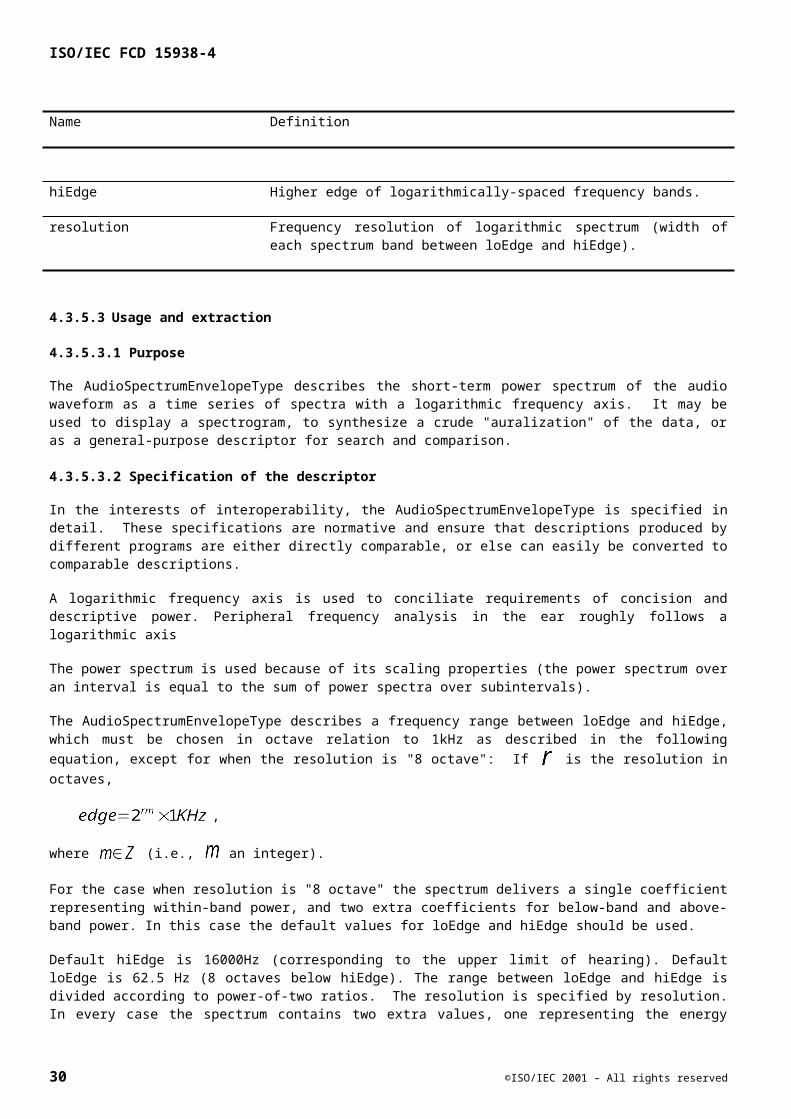
ISO/IEC FCD 15938-4

shape (corresponding to a noise-like or an impulse-like signal). A high deviation from a flat shape may indicate the presence of tonal components. The spectral flatness analysis is calculated for a number of frequency bands. It may be used as a feature vector for robust matching between pairs of audio signals.


The extraction of the AudioSpectrumFlatnessType can be efficiently combined with the extraction of the AudioSpectrumEnvelopeType and is done in several steps:

d) A spectral analysis of the input signal is performed using the procedure and parameters specified for the extraction of the AudioSpectrumEnvelopeType, but with a hop size corresponding to one full window length (i.e. no overlap between subsequent calculations).

e) The flatness measure is calculated (see next step) for a number of bands, as described by the attribute numBands. These bands are defined by a partitioning of the frequency range from 300 Hz to 6300 Hz into bands of equal width. The spectral coefficients (bins) corresponding to each transition frequency are determined as described for the extraction of the AudioSpectrumEnvelopeType.

f) For each band, the flatness measure is defined as the ratio of the maximum power spectrum coefficient (i.e. squared absolute value) and the mean of the power spectrum coefficients within the band. If no audio signal is present (i.e. the mean power is zero), a flatness measure value of 1 is returned.

4.3.9.4 Example

The following is an example instantiation of AudioSpectrumFlatnessType. Consider a series of calculated flatness measurements of 32 consecutive analysis frames. The following instantiation shows how to summarize these values by using the Min, Max, Mean and Variance fields of the SeriesOfVector datatype for a 4-band flatness descriptor:

<AudioD xsi:type="AudioSpectrumFlatnessType"> <SeriesOfVector> <Value vectorSize="4" totalSampleNum="128"> <Scaling ratio="64" elementNum="2"/> <Min dim="2 4"> 1.3 1.1 1.4 1.8 1.5 1.6 1.3 1.9 </Min> <Max dim="2 4"> 1.8 1.4 1.7 2.6 2.2 2.4 2.6 2.8 </Max> <Mean dim="2 4"> 1.6 1.35 1.5 2.3 1.8 2.1 1.8 2.4 </Mean> <Variance dim="2 4"> 0.5 0.11 0.76 0.42 0.87 0.32 0.31 0.43 </Variance> </Value> </SeriesOfVector> </AudioD>

4.3.10 AudioFundamentalFrequencyType

AudioFundamentalFrequencyType describes the fundamental frequency of the audio signal.

4.3.10.1 Syntax

   <complexType name="AudioFundamentalFrequencyType"> <complexContent>


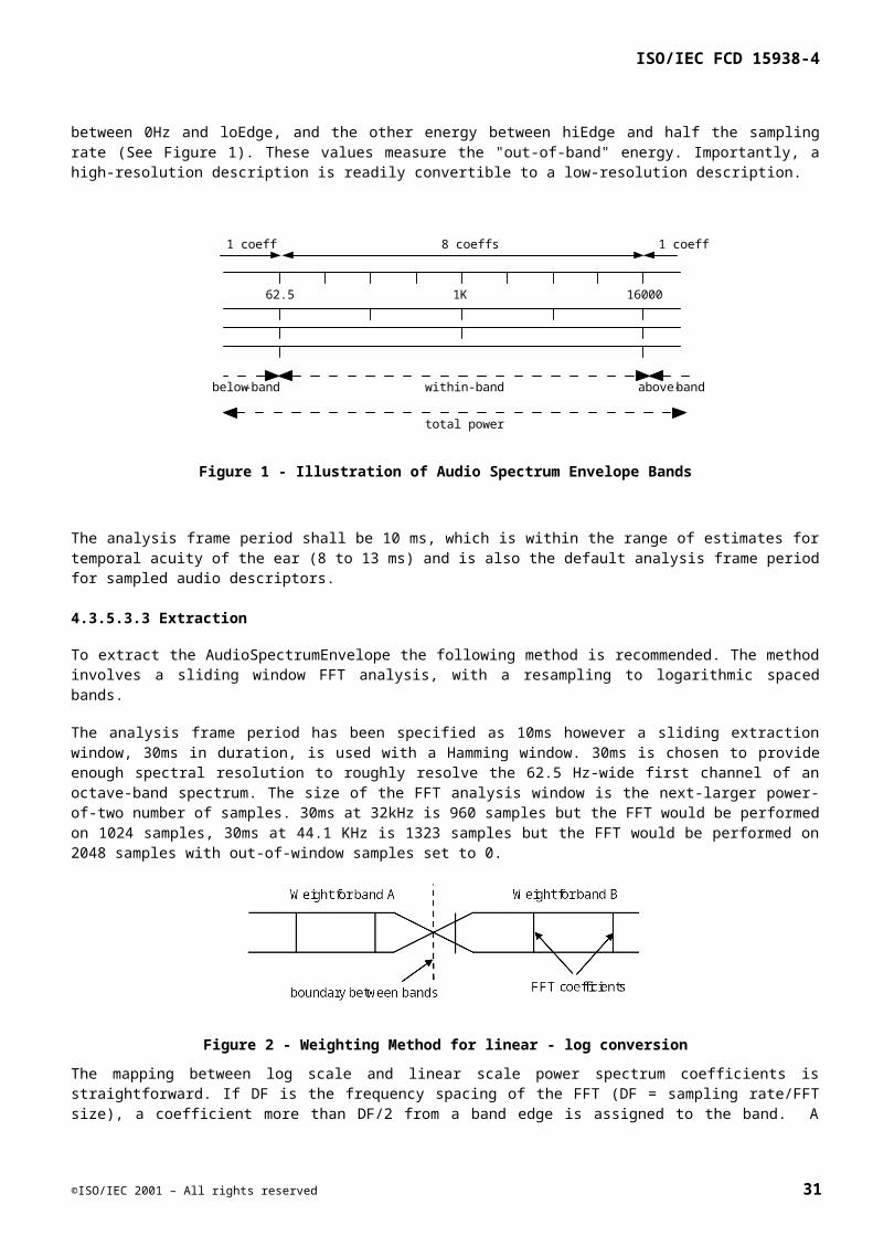
ISO/IEC FCD 15938-4

<extension base="mpeg7:AudioLLDScalarType"> <attribute name="loLimit" type="float" use="default" value="25"/> <attribute name="hiLimit" type="float" use="optional"/> </extension> </complexContent> </complexType>

4.3.10.2 Semantics

Name Definition

AudioFundamentalFrequencyType Description of the fundamental frequency of the audio signal.

loLimit Lower limit of search space, in Hz.

hiLimit Upper limit of search space, in Hz.



The extraction method is not specified in complete detail in order to promote choice of strategy. However the following shall be present in call cases.

The limits of the search range shall be specified using loLimit and hiLimit. The extraction method shall report a fundamental frequency for any signal that is periodic over the analysis interval with a fundamental within the search range.

The extraction method shall provide a confidence measure, between 0 and 1, to be used as a weight in scaling operations. Values of the estimate for which the weight is zero shall be considered non-periodic and ignored in similarity and scaling operations. The handling of non-zero values, that allow periodic values to be differentially weighted, is left up to the specific application.

One extraction method is detailed in Section . This is not the best method available but it gives reasonable estimates of the fundamental frequency in stationary signals.

4.3.10.3.2 Purpose

Fundamental frequency is a good predictor of musical pitch and speech intonation. As such it is an important descriptor of an audio signal. This descriptor is not designed to be a descriptor of melody, but it may nevertheless be possible to make meaningful comparisons between data labeled with a melody descriptor, and data labeled with fundamental frequency.


Fundamental frequency is complementary to the log-frequency logarithmic spectrum, in that, together with AudioHarmonicityType, it specifies aspects of the detailed harmonic structure of periodic sounds that the logarithmic spectrum cannot represent for lack of resolution. The inclusion of a confidence measure, using the 'Weight' field of the SeriesOfScalars is an important part of the design, that allows proper handling and scaling of portions of signal that lack clear periodicity.

4.3.11 AudioHarmonicityType

Check the min/maxOccurs of the elementsAudioHarmonicityType describes the degree of harmonicity of an audio signal.


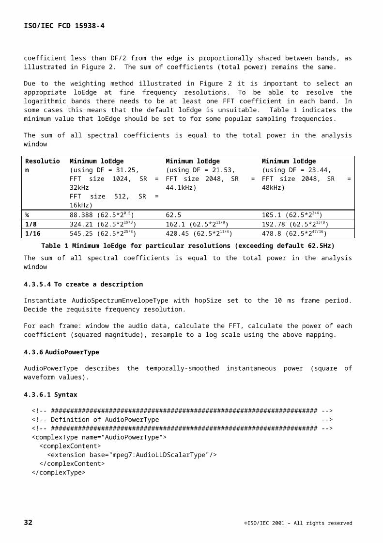
ISO/IEC FCD 15938-4

4.3.11.1 Syntax

    <complexType name="AudioHarmonicityType"> <complexContent> <extension base="mpeg7:AudioDType"> <sequence> <element name="HarmonicRatio"> <complexType> <complexContent> <extension base="mpeg7:AudioLLDScalarType"/> </complexContent> </complexType> </element> <element name="UpperLimitOfHarmonicity"> <complexType> <complexContent> <extension base="mpeg7:AudioLLDScalarType"/> </complexContent> </complexType> </element> </sequence> </extension> </complexContent> </complexType>

4.3.11.2 Semantics

Name Definition

AudioHarmonicityType Description of the spread of the log-frequency power spectrum.

HarmonicRatio Description of the ratio of harmonic power to total power.

UpperLimitOfHarmonicity The frequency beyond which the spectrum cannot be considered harmonic.



AudioHarmonicityType contains two measures: HarmonicRatio, and UpperLimitOfHarmonicity.

HarmonicRatio is loosely defined as the proportion of harmonic components within the power spectrum. It is derived from the output/input power ratio of a time domain comb filter tuned to the period 1/F0 of the signal. In order to avoid dependency on the actual F0 estimate, the algorithm produces its own estimate by searching for the minimum output of such a comb filter. The algorithm is:

a) Calculate:

Where


ISO/IEC FCD 15938-4

i) s is the audio signal

ii) m =I*n; i = 0,M-1

iii) M = number of frames

iv) k = 1,K

v) fs = sampling frequency

vi) w = maximum expected fundamental period (by default: 40ms)

vii) t = analysis window size (by default: 10ms)

viii) K = w*fs

ix) n = t*fs

b) Choose the maximum in each frame

This value is 1 for a purely periodic signal, and it will be close to 0 for white noise. The estimate can be refined by replacing each local maximum of by the maximum of a 3-point parabolic fit centered upon it.

UpperLimitOfHarmonicity is loosely defined as the frequency beyond which the spectrum cannot be considered harmonic. It is calculated based on the power spectra of the original and comb-filtered signals. The algorithm is:

c) Determine the combed signal

where

… is the optimal gain

K is the lag corresponding to the maximum cross correlation ( ), and the fundamental period estimate.

d) Calculate the DFTs of the signal s(j) and the comb-filtered signal c(j), using a 30 ms window shaped as a raised cosine. If K is fractionary, s(j-K) is calculated by linear interpolation. Calculate power spectra, and group the components below 62.5 Hz as explained for AudioSpectrumEnvelopeType.

e) For each frequency f calculate the sum of power beyond that frequency, for both the original and comb-filtered signal, and take their ratio.

where p(f) and p'(f) are the power spectra of the unfiltered and filtered signal respectively, and is the maximum frequency of the DFT.

f) Starting from and moving down in frequency, find the greatest frequency for which this ratio is smaller than a threshold (0.5). If that frequency is 0, replace it by 31.25 Hz.


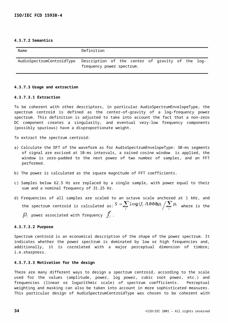
ISO/IEC FCD 15938-4

g) Convert this value to an octave scale based on 1 kHz.

4.3.11.3.2 Purpose

A harmonicity measure allows distinguishing between sounds that have a harmonic spectrum (musical sounds, voiced speech, etc.) and those that have a non-harmonic spectrum (noise, unvoiced speech, dense mixtures of instruments, etc.).


Together with AudioFundamentalFrequencyType, AudioHarmonicityType describes the harmonic structure of sound. These features are orthogonal and complementary with a descriptor such as AudioSpectrumEnvelopeType. The exact definitions of the measures (HarmonicRatio and UpperLimitOfHarmonicity) are designed to be easy to extract, and coherent with the definitions of other descriptors (most of which are based on power).

4.3.12 TimbreDescriptorType

4.3.12.1 Introduction

The TimbreDescriptorType, and all of the following descriptors that inherit from it, are distinct from the preceeding low-level descriptors. In the context of the high-level Timbre description tools (section 5.2), they are intended to be descriptors that apply to an entire audio segment, rather than being primarily sampled types.

All timbre descriptors are defined as subtypes of TimbreDescriptorType.

4.3.12.2 Syntax

   <complexType name="TimbreDescriptorType" abstract="true"> <complexContent> <extension base="mpeg7:AudioLLDScalarType"> <attribute name="confidence" type="mpeg7:zeroToOneType"/> </extension> </complexContent> </complexType>

4.3.12.3 Semantics

Name Definition

confidence The confidence gives a measure of the quality of the estimation of each of the descriptors, and therefore also of the reliability of the results one can have by using the descriptors.

Range: [0,1]


As many of the timbre descriptors rely on a previous estimation of the fundamental frequency and the harmonic peaks of the spectrum or on the temporal signal envelope (Figure 3), the extraction of these is explained first rather than repeating it for each the timbre descriptors.


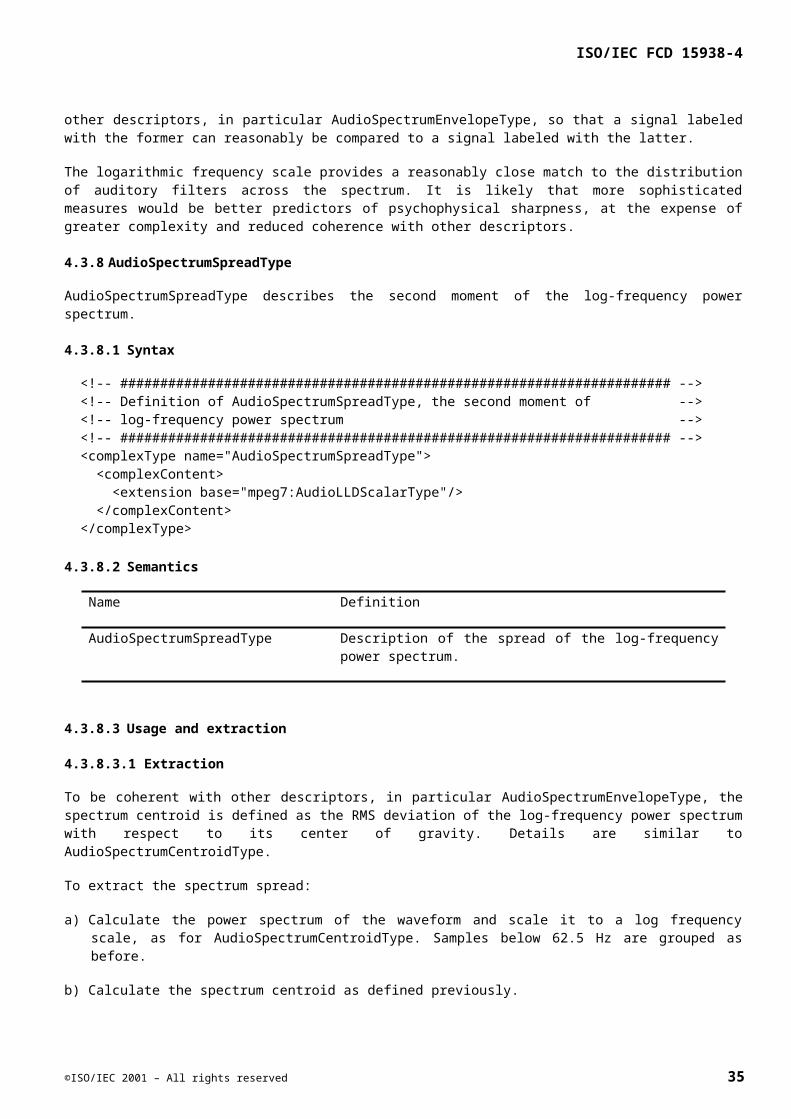
ISO/IEC FCD 15938-4

Figure 3 — Space 1 Timbre Descriptors Estimation

4.3.12.5 Estimation of spectral parameters

The calculation of the fundamental frequency and the harmonic peaks is required before the calculation of each of the instantaneous harmonic spectral features, including centroid, deviation, spread and variation. The timbre descriptors have been designed for specific use upon harmonic signals, such as a monophonic musical signal. Each descriptor describes a sound segment. An example of a sound segment would be a single note played on a clarinet.

4.3.12.5.1 Estimation of the fundamental frequency f0 (informative)

The fundamental frequency is the frequency that best explains the periodicity of a signal. While numerous methods have been proposed in order to estimate it, one can simply compute the local normalized auto-correlation function of the signal and take its first maximum in order to estimate the local fundamental period. The local fundamental frequency is then estimated by the inverse of the time corresponding to the position of this maximum. An alternate method is that which is described in Section .

4.3.12.5.2 Harmonic Peaks Detection (informative)

The harmonic peaks are the peaks of the spectrum located “around” the multiple of the fundamental frequency of the signal. The term “around” is used in order to take into account the slight variations of harmonicity of some sounds (piano for example). While numerous methods have been proposed in order to estimate the harmonic peaks, one can simply look for the maxima of the amplitude of the Short Time Fourier Transform (STFT) close to the multiples of the fundamental frequency. The frequencies of the harmonic peaks are then estimated by the positions of these maxima while the amplitudes of these maxima determine their amplitudes.


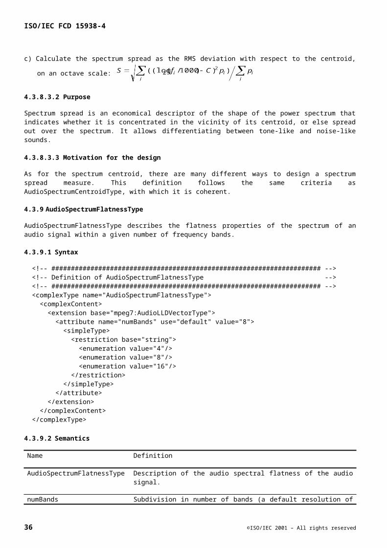
ISO/IEC FCD 15938-4

Figure 4 Harmonic Peaks Detection (informative)

Suggested algorithm for harmonic peaks detection (informative) If X(k), k in [1,N] denotes the values of the bins of the STFT of size N

If f0 (units = Hz) denotes the estimated fundamental frequency,

If sr denotes the sampling rate

If floor(x) = k, where k≤x , k an integer

If ceil(x) = m, where m≥x, m an integer

If abs(x) denotes the mapping function of complex value x to its polar amplitude valueThe hth harmonic peaks of the signal can be estimated by looking at the maximum of the spectrum X(K) in the region K, where K is defined as [floor(h*f0-c*f0),ceil(h*f0+c*f0)].

The parameter c in [0, 0.5], determines the tolerated non-harmonicity. A value of c=0.15 is recommended.

4.3.12.5.3 Suggested Analysis Parameters for the spectral parameters: (informative)

type of the analysis window: hamming

size of the analysis window: 8 fundamental period

hop size: 4 fundamental period

OR

type of the analysis window: hamming

size of the analysis window: 30ms

hop size: 10ms


ISO/IEC FCD 15938-4

4.3.12.5.4 Term definitions

The following definitions are also given in the high-level Timbre section (5.2). These clearly need to be harmonised and placed in the front section of the document, but consideration must also be given to how these definitions interact throughout the document.Frame: A Frame is defined as a short period of time of the signal on which the instantaneous analysis if perform. For a signal, noted s(t) (in continuous time noted t), and for an analysis window of type hamming, noted h(t) and of temporal length L, the fth signal frame is defined as

where S is the hop size

Hop size: The hop size defines the temporal distance between two successive analyses.

Running window analysis: A running window analysis is an analysis obtained by mutliplying the signal by a window function which is shifted along time by integer multiple of a parameter called the hop size. For a window function h(t), and a hop size S, the fth shifting of the window is equal to h(t-fS).

Instantaneous values: For the instantaneous values of the Timbre descriptors based on harmonic peaks estimation (IHSC, IHSD, IHSS, IHSV), corresponds to the analysis on a frame level. The values of the global values of the Timbre descriptors based on harmonic peaks estimation (HSC, HSD, HSS, HSV) corresponds to the average over all frames of the segment of the instantaneous values

4.3.12.6 Estimation of temporal parameters

4.3.12.6.1 Log-Attack-Time and Temporal Centroid: Signal envelope

While numerous methods have been proposed in order to compute the signal envelope, one can simply use a signal’s power function over time. This function can be estimated by computing the local mean square value of the signal amplitude within a running window.

4.3.13 LogAttackTimeType

4.3.13.1 Syntax

   <complexType name="LogAttackTimeType"> <complexContent> <extension base="mpeg7:TimbreDescriptorType"/> </complexContent> </complexType>

4.3.13.2 Semantics

Name Definition

LogAttackTime The LogAttackTime (LAT) is defined as the logarithm (decimal base) of the time the signal starts to the time it reaches its stable part.

Unit: [log10 sec]

Range: [log10(1/sr),determined by the length of the signal]


ISO/IEC FCD 15938-4

Where sr stands for sampling rate



a) Estimate the temporal signal envelope over the time of the segment

b) Compute the LAT as following

where

T0 is the time the signal starts;

T1 is the time the signal reaches its sustained part (harmonic space) or maximum part (percussive space).

T0t

Signal envelope(t)

T1

Figure 5 — Illustration of log-attack time

T0 can be estimated as the time the signal envelope exceeds 2% of its maximum value. T1 can be estimated, simply, as the time the signal envelope reaches its maximum value.


The ‘attack’ of a sound is the first part of a sound, before a real note develops.

4.3.14 HarmonicSpectralCentroidType

4.3.14.1 Syntax

   <complexType name="HarmonicSpectralCentroidType"> <complexContent> <extension base="mpeg7:TimbreDescriptorType"/> </complexContent> </complexType>


ISO/IEC FCD 15938-4

4.3.14.2 Semantics

Name Definition

HarmonicSpectralCentroid The HarmonicSpectralCentroid (HSC) is computed as the average over the sound segment duration of the instantaneous harmonic spectral centroid (IHSC) within a running window. The IHSC is computed as the amplitude (linear scale) weighted mean of the harmonic peaks of the spectrum.

Unit: [Hz]

Range: [0,sr/2]


The HSC may be extracted using the following algorithm

a) Estimate the harmonic peaks over the sound segment

b) Calculate the IHSC for each frame as follows:

where

A(frame,harmo) is the amplitude (linear scale) of the harmonic peak number “harmo” at the frame number “frame”

f(frame,harmo) is the frequency (linear scale) of the harmonic peak number “harmo” at the frame number “frame”

nb_harmo is the number of harmonics taken into account

c) Calculate the HSC for the sound segment as follows:

where

nb_frames is the number of frames in the sound segment

4.3.15 HarmonicSpectralDeviationType

4.3.15.1 Syntax

 


ISO/IEC FCD 15938-4

 <complexType name="HarmonicSpectralDeviationType"> <complexContent> <extension base="mpeg7:TimbreDescriptorType"/> </complexContent> </complexType>

4.3.15.2 Semantics

Name Definition

HarmonicSpectralDeviation The HarmonicSpectralDeviation (HSD) is computed as the average over the sound segment duration of the instantaneous HSD (IHSD) within a running window. The IHSD is computed as the spectral deviation of amplitude (logarithmic scale) components from a global spectral envelope.

Unit: [-]

Range: [0,1]


The HSD may be extracted using the following algorithm


b) Estimate the spectral envelope (SE)

(Informative) The local Spectral Envelope (linear scale) can be approximated by taking the mean of the amplitude (linear scale) of the three adjacent harmonic peaks. To evaluate the ends of the envelope simply use the mean of the amplitude of two adjacent harmonic peaks.

For harmo = 1

For harmo = 2 to nb_harmo-1

For harmo = nb_harmo

where



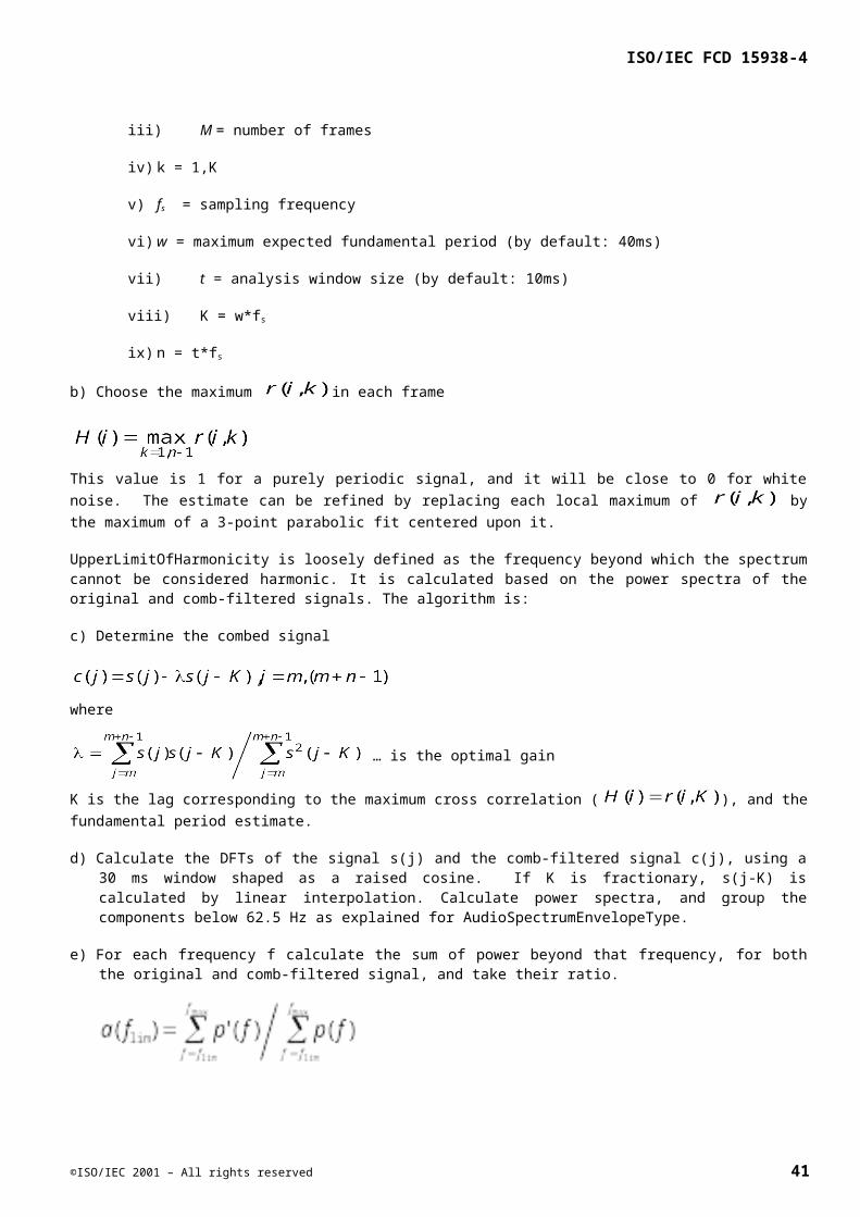
ISO/IEC FCD 15938-4

d) Calculate the IHSD for each frame as follows:

where

A(frame,harmo) is the amplitude (logarithmic scale) of the harmonic peak number “harmo” at the frame number “frame”

SE(frame,harmo) is the local Spectral Envelope (amplitude in logarithmic scale) around the harmonic peak number harmo


e) Calculate the HSD for the sound segment as follows:

where


4.3.16 HarmonicSpectralSpreadType

4.3.16.1 Syntax

   <complexType name="HarmonicSpectralSpreadType"> <complexContent> <extension base="mpeg7:TimbreDescriptorType"/> </complexContent> </complexType>

4.3.16.2 Semantics

Name Definition

HarmonicSpectralSpread The HarmonicSpectralSpread (HSS) is computed as the average over the sound segment duration of the instantaneous HSS (IHSS) within a running window.

The IHSS is computed as the amplitude (linear scale) weighted standard deviation of the harmonic peaks of the spectrum, normalized by the IHSC.


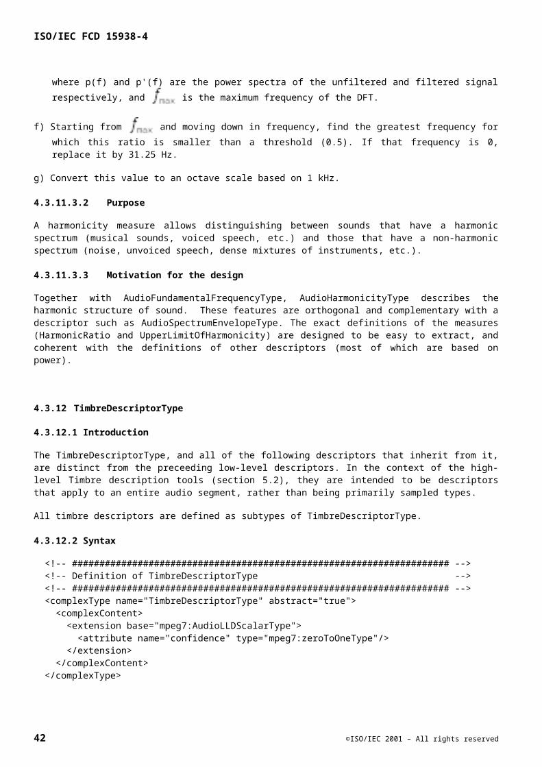
ISO/IEC FCD 15938-4

Units: [-]

Range: [0,1]


The HSS may be extracted using the following algorithm


b) Estimate the IHSC of each frame

c) Calculate the IHSS for each frame as follows:

where


f(frame,harmo) is the frequency (linear scale) of the harmonic peak number “harmo” at the frame number “frame”


d) Calculate the HSS for each sound segment as follows:

where


4.3.17 HarmonicSpectralVariationType

4.3.17.1 Syntax

   <complexType name="HarmonicSpectralVariationType"> <complexContent> <extension base="mpeg7:TimbreDescriptorType"/> </complexContent> </complexType>


ISO/IEC FCD 15938-4

4.3.17.2 Semantics

Name Definition

HarmonicSpectralVariation The HarmonicSpectralVariation (HSV) is defined as the mean over the sound segment duration of the instantaneous HSV (IHSV).

The IHSV is defined as the normalized correlation between the amplitude (linear scale) of the harmonic peaks of two adjacent frames.

Units: [-]

Range: [0,1]


The HSV may be extracted using the following algorithm


b) Calculate the IHSV for each frame as follows:

where



c) Calculate the HSV for the sound segment as follows:

where


4.3.18 SpectralCentroidType

4.3.18.1 Syntax

  


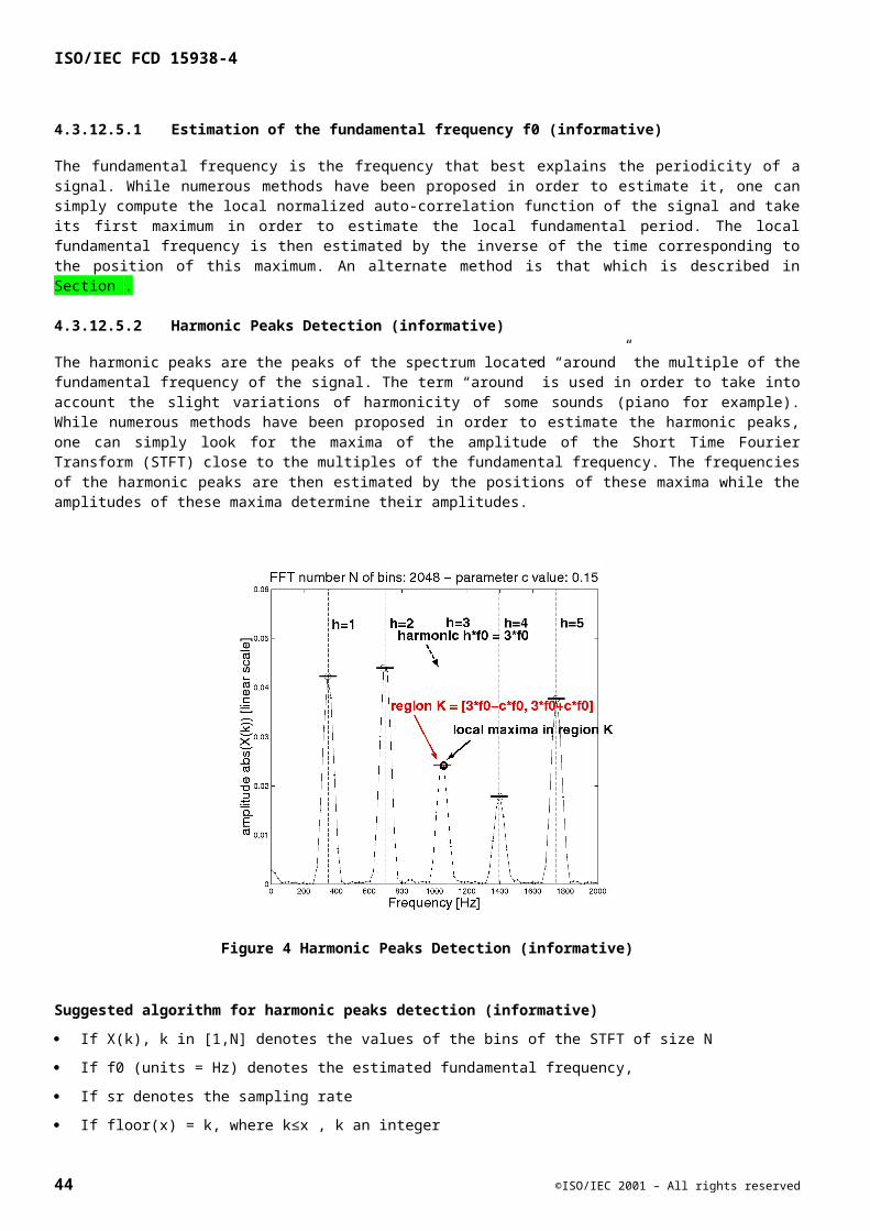
ISO/IEC FCD 15938-4

<complexType name="SpectralCentroidType"> <complexContent> <extension base="mpeg7:TimbreDescriptorType"/> </complexContent> </complexType>

4.3.18.2 Semantics

Name Definition

SpectralCentroid The SpectralCentroid (SC) is computed as the power weighted average of the frequency of the bins in the power spectrum.

Unit: [Hz]

Range: [0,sr/2]



The SC may be extracted using the following algorithm

a) Determine the power spectrum over the sound segment

(Informative) While numerous methods have been proposed in order to compute the power spectrum, one can simply use the Welch method (averaged periodogram) both for harmonic and percussive sounds.

f) Calculate the ISC for each frame as follows:

where:

f(k) stands for the frequency of the kth spectrum coefficient

S(k) corresponds to its associated power

g) Calculate the SC for the sound segment as follows:

where



ISO/IEC FCD 15938-4

4.3.19 TemporalCentroidType

4.3.19.1 Syntax

   <complexType name="TemporalCentroidType"> <complexContent> <extension base="mpeg7:TimbreDescriptorType"/> </complexContent> </complexType>

4.3.19.2 Semantics

Name Definition

TemporalCentroid The TemporalCentroid (TC) is defined as the time averaged over the energy envelope.

Unit: [sec]

Range: [0,determined by the length of the signal]


The TC may be extracted using the following algorithm

a) Calculate the Signal Envelope (as described in 4.3.12.6.1)

b) Calculate the TC for as follows:

where

envINST means the Instantaneous Energy Envelope.

Sr is the Sampling Rate.

4.3.20 AudioSpectrumBasisType

The AudioSpectrumBasis descriptor contains basis functions that are used to project high-dimensional spectrum descriptions into a low-dimensional representation contained by the AudioSpectrumProjection descriptor. This reduced representation is suitable, for example, for use with probability model classifiers that


ISO/IEC FCD 15938-4

require input features to be of fewer than 10 dimensions for successful performance or it may also be used for describing independent component spectrograms that constitute a spectrum.

In the sections below normative methods are given for reducing the dimensions of AudioSpectrumEnvelope descriptions. There are many uses for dimensionality reduction, and these tools play a substantial role in the SoundRecognition tools. Spectrogram summarization applications are described in the Usage section for AudioSpectrumProjection.

4.3.20.1 Syntax

   <complexType name="AudioSpectrumBasisType"> <complexContent> <extension base="mpeg7:AudioDType"> <sequence> <element name="BasisFunctions" type="mpeg7:DoubleMatrixType"/> </sequence> <attributeGroup ref="mpeg7:audioSpectrumAttributeGrp"/> </extension> </complexContent> </complexType>

4.3.20.2 Semantics

Name Definition

AudioSpectrumBasisType Spectral basis vectors contained in the columns of a matrix

AudioSpectrumAttrGroup AudioSpectrumEnvelope parameters used in obtaining the spectral basis vectors.

4.3.20.3 Example Instantiation

<AudioD xsi:type="AudioSpectrumBasisType" loEdge="62.5" hiEdge="8000" resolution="1/4 octave"> <BasisFunctions> <Matrix dim="31 5"> 0.26 -0.05 0.01 -0.70 0.44 0.34 0.09 0.21 -0.42 -0.05 0.33 0.15 0.24 -0.05 -0.39 0.33 0.15 0.24 -0.05 -0.39 0.27 0.13 0.16 0.24 -0.04 0.27 0.13 0.16 0.24 -0.04 0.23 0.13 0.09 0.27 0.24 0.20 0.13 0.04 0.22 0.40 0.17 0.11 0.01 0.14 0.37 . . . </Matrix> </BasisFunctions> </AudioD>


ISO/IEC FCD 15938-4

4.3.20.4 Extraction

The following section outlines the normative methods for extracting basis functions from a spectrum. Some details of extraction are indicated to be optional with no loss of compatibility between implementations.

To extract a reduced-dimension basis for AudioSpectrumEnvelope perform the following steps:

a) Instantiate an AudioSpectrumEnvelope descriptor with spectral data using the extraction method defined in AudioSpectrumEnvelopeType. The resulting data will be a SeriesOfVectors with M frames and N frequency bins.

b) For each spectral frame, represented by a vector in the SeriesOfVectors, normalize the frame by the total power of the frame (i.e. the sum of the vector elements):

This is a normative extraction step if the reduced-dimension features are to be used with a probability classifier.

c) Place each vector row-wise into a matrix. The size of the resulting matrix is M x N where M is the number of time frames and N is the number of frequency bins. The matrix will have the following structure:

d) Extract a basis using a singular value decomposition (SVD) such as is commonly implemented as a built-in functions in many software packages using the command [U,S,V] = SVD(X,0). Use the economy SVD when available since the row-basis functions are not required and this will increase extraction efficiency. The SVD factors the matrix from step 3 in the following way:

where X is factored into the matrix product of three matrices; the row basis U, the diagonal singular value matrix S and the transposed column basis functions V. AudioSpectrumBasisType describes the basis functions contained in U. Reduce the basis by retaining only the first K basis functions, i.e. the first K columns of V:

K is typically in the range of 3-10 basis functions for feature-based applications. To calculate the proportion of information retained for K basis functions use the singular values contained in matrix S:


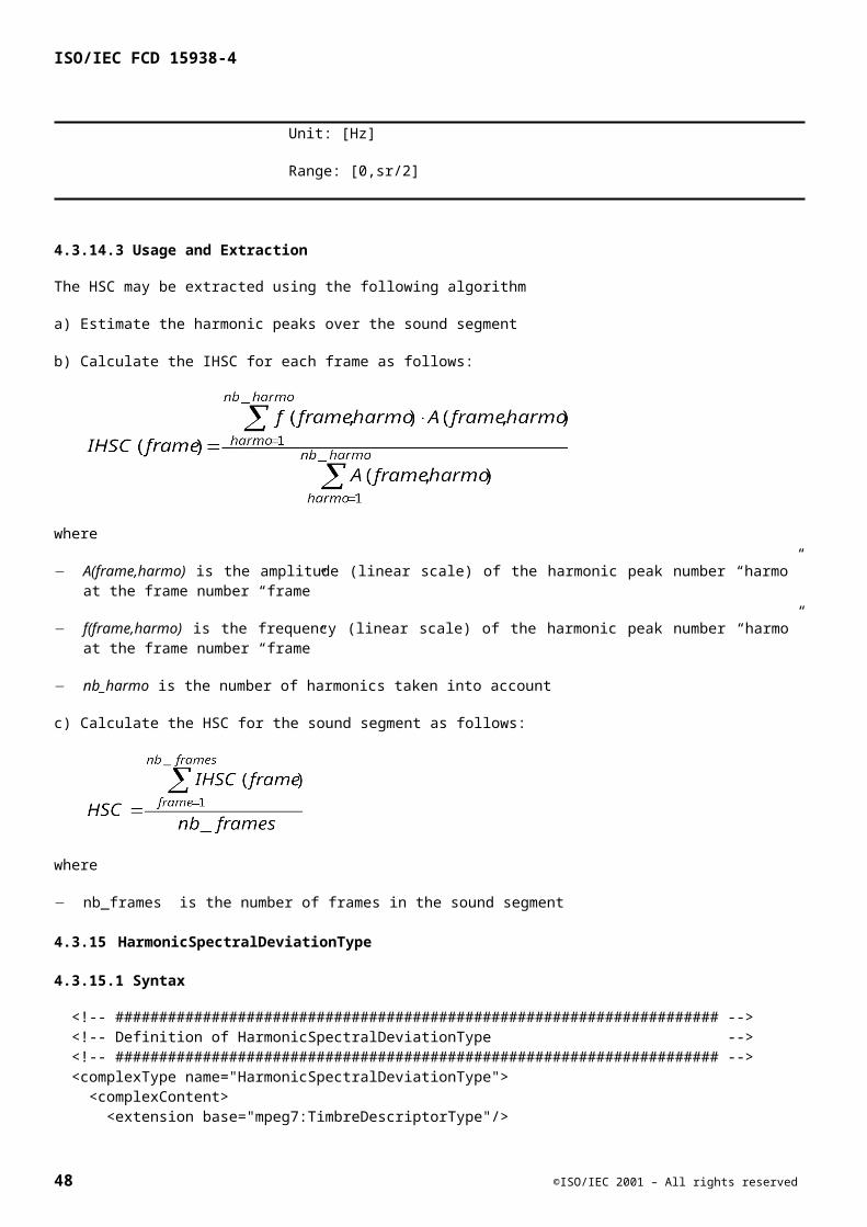
ISO/IEC FCD 15938-4

where I(K) is the proportion of information retained for K basis functions and N is the total number of basis functions which is also equal to the number of spectral bins. The SVD basis functions are stored in the columns of the matrix contained in the AudioSpectrumBasisType descriptor.

e) (Optional). After extracting the reduced SVD basis, V, a further step consisting of basis rotation to directions of maximal statistical independence is often desirable. This is necessary for displaying independent components of a spectrogram and for any application requiring maximum separation of features.

To find a statistically independent basis using the basis functions obtained in step 4, use one of the well-known, widely published independent component (ICA) algorithms such as JADE or FastICA; see Cardoso, J.F. and Laheld, B.H. (1996), Equivariant adaptive source separation, IEEE Trans. On Signal Processing, 4:112-114 or Hyvarinen, A. (1999), Fast and robust fixed-point algorithms for independent component analysis, IEEE Trans. On Neural Networks, 10(3):626-634.

The following use of ICA will factor a set of vectors into statistically independent vectors:

where the new basis is obtained as the product of the SVD input vectors and the psuedo-inverse of the estimated mixing matrix A given by most ICA algorithms, e.g.:

The ICA basis is the same size as the SVD basis and is stored in the columns of the matrix contained in the AudioSpectrumBasisType descriptor. The retained information ratio, I(K), is equivalent to the SVD when using the given extraction method.

Figure 6 Extraction method for AudioSpectrumBasisType and AudioSpectrumProjectionType

4.3.20.5 AudioSpectrumBasisType Usage (informative)

See informative usage section for AudioSpectrumProjectionType below.

4.3.21 AudioSpectrumProjectionType

This descriptor is the compliment to AudioSpectrumBasisType and is used to represent low-dimensional features of a spectrum after projection against a reduced basis. These two types are always used together. Informative applications for both descriptors are given in the usage section below.


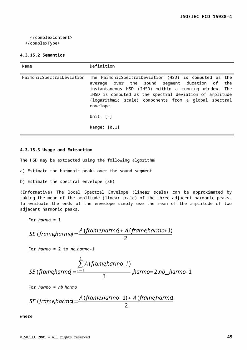
ISO/IEC FCD 15938-4

4.3.21.1 Syntax

   <complexType name="AudioSpectrumProjectionType"> <complexContent> <extension base="mpeg7:AudioLLDVectorType"/> </complexContent> </complexType>

4.3.21.2 Semantics

Name Definition

SpectrumBasisProjectionType Basis projected spectrum represented as a series of vectors

4.3.21.3 Extraction

Figure 6 shows the extraction system diagram for both AudioSpectrumBasis and AudioSpectrumProjection. To perform extraction for SpectrumBasisProjectionType follow steps 1-3 described above for AudioSpectrumBasis extraction, this produces a spectrum matrix. The only further requirement is to multiply the spectrum matrix with the basis vectors obtained in step 4 or, optionally, step 5. The method is the same for both SVD and ICA basis functions:

where Y is a matrix consisting of the reduced dimension features after projection of the spectrum against the basis V.

For independent spectrogram reconstruction and viewing extract the non-normalized spectrum projection by skipping the normalization step (2) in AudioSpectrumBasis extraction. Thus:

Now, to reconstruct an indpendent spectrogram component use the individual vector pairs, corresponding to the Kth vector in AudioSpectrumBasis and AudioSpectrumProjection, and apply the reconstruction equation:

where the + operator indicates the transpose for SVD basis functions (which are orthonormal) or the pseudo-inverse for ICA basis functions (non-orthogonal).

4.3.21.4 Usage (informative)

4.3.21.4.1 Application: Spectrogram summarization by independent components.

One of the uses for these descriptors is to efficiently represent a spectrogram with much less data than a full spectrogram. Using an independent component basis, individual spectrogram reconstructions generally correspond to source objects in the spectrogram. The following examples are taken from a recording of a song featuring guitar, drums, hi-hat, bass guitar, and organ. Figure 7 shows the original full-bandwidth spectrogram. shows a single independent component reconstruction. Figure 9 shows reconstruction using 4 independent components, and


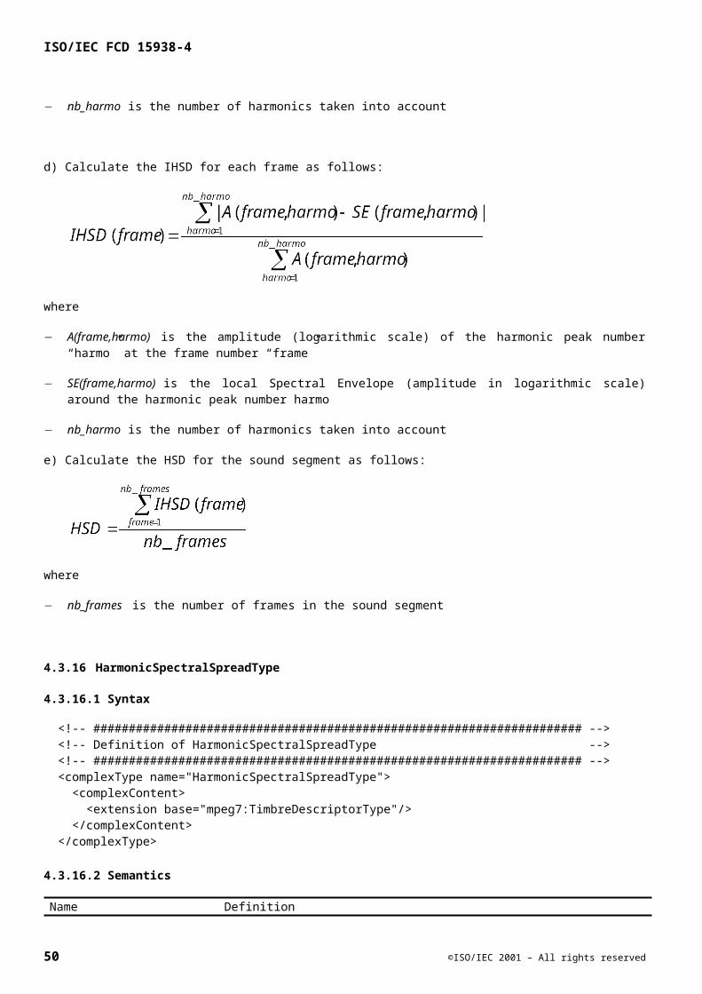
ISO/IEC FCD 15938-4

Figure 10 shows a 10-component reconstruction. The data ratio, R, between the reduced-dimension spectrum and the full-bandwidth spectrum is:

where K is the number of basis components, M is the number of frames in the spectrogram and N is the number of frequency bins. For example, a 5-component reconstruction of 500 frames of a 64-bin spectrogram leads to a data reduction of ~11:1.

Figure 7 AudioSpectrumEnvelope description of a pop song. The required data storage is NM values where N is the number of spectrum bins and M is the number of time points.


ISO/IEC FCD 15938-4

Figure 8 One basis component reconstruction showing repeating individual guitar notes. The leftmost vector is the first AudioSpectrumBasis vector and the topmost vector is the first AudioSpectrumProjectionVector. The two are combined using the reconstruction equation given above. The required data storage is (M+N) values.

Figure 9 Four basis component reconstruction showing more guitar notes. The required data storage is 4 (M+N) values.


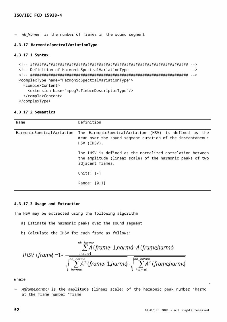
ISO/IEC FCD 15938-4

Figure 10 10-basis component reconstruction showing most of the detail of the original spectrogram including guitar, bass guitar, hi-hat and organ notes. The required data storage is 10(M+N) values.

4.3.21.4.2 Application: Uncorrelated Features for Sound Recognition

This application is covered in detail in the Sound Recognition tools section below. The reader is refered to the informative section of Sound Recognition tools for information on how to use AudioSpectrumBasisType and AudioSpectrumProjectionType as uncorrelated features for automatic classification of sound.


ISO/IEC FCD 15938-4

4.4 Silence

4.4.1 Introduction

The Silence Descriptor describes a perceptual feature of a sound track capturing the fact that no significant sound is occurring in this segment. It is useful for the segmentation of audio material into subparts, giving access to its physical structure.

The basic information of the description of a silent segment is the start time and the duration, which is given by times in the audio segment to which the silence descriptor is attached. The silence segments themselves are either given for the whole segment or as a TimeMask for the segment.

4.4.2 SilenceHeaderType

4.4.2.1 Syntax

   <complexType name="SilenceHeaderType"> <complexContent> <extension base="mpeg7:HeaderType"> <sequence> <element name="minDuration" type="mpeg7:mediaDurationType"/> </sequence> <attribute name="id" type="ID"/> </extension> </complexContent> </complexType>

4.4.2.2 Semantics

Name Definition

SilenceHeaderType Information shared by many silence descriptors

minDuration The minDuration attribute is used to communicate a minimum temporal threshold determining whether a signal portion is identified as a silent segment (see information on extraction process). The minDuration element is usually applied uniformly to a complete segmentDecomposition as a parameter for the extraction algorithm.

id Unique identifier to reference the header

4.4.3 SilenceType

4.4.3.1 Syntax

   <complexType name="SilenceType"> <complexContent> <extension base="mpeg7:AudioDType"> <attribute name="confidence" type="mpeg7:zeroToOneType" use="default" value="1.0"/>


ISO/IEC FCD 15938-4

<attribute name="minDurationRef" type="uriReference" use="optional"/> </extension> </complexContent> </complexType>

4.4.3.2 Semantics

Name Definition

confidence The confidence attribute measures how confident the detection process is that the segment is containing silence. Unit: None

Range: [0,1]minDurationRef Reference to minDuration information in a SilenceHeader


ISO/IEC FCD 15938-4

4.4.4 Usage, examples and extraction (informative)

Silence can be regarded as a semantic concept. For example, a long silent period in a movie may signify that something important is about to happen, such as falling in love or increasing tension for an expected event. Together with speech, music and ambient sound descriptors, the silence descriptors captures the basic semantic events occurring in audio material.

Silence can be used to segment audio materials at varying levels of detail depending on the parameters used during the detection phase. For example, a high threshold may be used to detect long pauses between sentences as silence while tolerating shorter breaks between phrases. A lower threshold may be used to identify phrasal pauses or even pauses between words. Similarly, pauses in music pieces of varying length may be determined. In this way, audio material may be split up into parts that reflect its physical structure. Segmentation is an important prerequisite for further classification of the identified segments.

Target applications are:

Direct access to semantic segmentations/events of audio material.

Segmentation tools for annotation and retrieval, e.g. news story segmentation, captioning software.

The silence extractor can be implemented in various ways. One possible implementation of a confidence measure is to investigate the calculated (loudness) function over time with respect to an assumed (loudness) threshold, see informative description of an example silence detection algorithm. The confidence measure can e.g. be calculated from the ratio of the area under the (loudness) threshold and the area under the (loudness) curve, clipped to the range [0 ... 1].

4.4.4.1 Description of a silence detection algorithm

This section describes how a silence detector may be implemented by using an FFT-based algorithm to calculate the sliding loudness of the signal. An implementation of a simple silence detection algorithm is described.

Figure 11 — Loudness based Silence Detector

The signal processing is carried out in several steps:

a) Sliding short Time Fourier Transform (STFT)

b) Filtering with outer ear transfer function

c) Summing the energy into 1 bark wide bands

d) Calculating masking threshold, considering threshold in quiet and temporal masking

e) Calculating partial loudness and overall loudness

f) Detecting silence segments by a suitable thresholding process

Descriptions for steps (a) – (d) can be found in ISO/IEC 11172-3, Annex D or ISO/IEC 13818-7, Annex B.


ISO/IEC FCD 15938-4

A thresholding process could employ several parameters, such as silence level thresholds and a minimum duration for which those thresholds are to be exceeded for a change in detector output. Such a scheme is illustrated by the following figure:

Figure 12 — Silence thresholds

Depending on the type and complexity of the audio signals, it may be necessary to automatically adapt the thresholding process to the characteristics of the background noise. An “intelligent” silence detector could additionally support perceptually-based concepts for silence, such as voice activity measures etc..

4.4.4.2 Example

<AudioSegment> <Header xsi:type="SilenceHeaderType" id="shOne"> <minDuration>PT3N10F</minDuration> </Header> <MediaTime> <MediaRelTimePoint timeBase="MediaLocator[1]">P0S</MediaRelTimePoint> <MediaDuration>PT28S3N10F</MediaDuration> </MediaTime> <AudioD xsi:type="SilenceType" minDurationRef="shOne" confidence="0.5"/> </AudioSegment>


ISO/IEC FCD 15938-4

5 High Level Tools

5.1 Introduction

Introduction needs expandingThis section contains descriptors and description schemes which are broadly classed as “high level”; that is, they are either structural or application oriented. In some cases, they use tools defined in the audio framework section of this document. Much use is made of tools defined in the multimedia description schemes part of the standard.

5.2 Timbre

5.2.1 Introduction

Timbre Descriptors aim to describe perceptual features of instrument sounds. Timbre is currently defined in the literature as the perceptual features that make two sounds having the same pitch and loudness sound different. The aim of the Timbre DS is to describe these perceptual features with a reduced set of descriptors. The descriptors relate to notions such as “attack”, “brightness” or “richness” of a sound. The Timbre DS use the low-level audio Descriptors of TimbreDescriptorType described above.

Families of sounds and the three TimbreType:

“Timbre similarity” refers to the way human listeners consider two sounds as close whatever classes they belong to and whatever pitch and loudness. Human perception of similarity between sounds is a rather complex mechanism, which involves taking into account several parameters that determine several perceptual dimensions in a possibly complex way. Human listeners will use different perceptual dimensions depending on the family of sounds being heard. For example, the harmonicity feature may be used to distinguish harmonic and non-harmonic sounds, but is unlikely to be important to distinguish sounds within each of these families.

For this reason we distinguish four different families of sounds for the monophonic, non-mixed, non-layered instrument sounds. These families correspond to the main perceptual categories of musical sounds distinguished by the following factors (see Table 1):

Harmonic: relates to the property of periodicity of a signal (the harmonicity relations between the components of the spectrum a signal; distinguishes harmonic from inharmonic and noisy signals).

Sustained: relates to the duration of excitation of the sound source (distinguishes sustained from impulsive signals).

Coherent: relate to the temporal behaviour of the spectral component of a signal (distinguishes frequency spectra with prominent components from noisy spectra).

Sound families Harmonic Sounds 2 Percussive Sounds 4

Sounds characteristics Sustained

Harmonic

Coherent

Sustained

Non-Harmonic

Coherent

Non-Sustained Sustained

Non-Coherent

Examples of sounds belonging to the family

violin, flute, … bell, triangle snare, claves, … cymbals, white noise, …

TimbreType HarmonicInstrument

PercussiveInstument


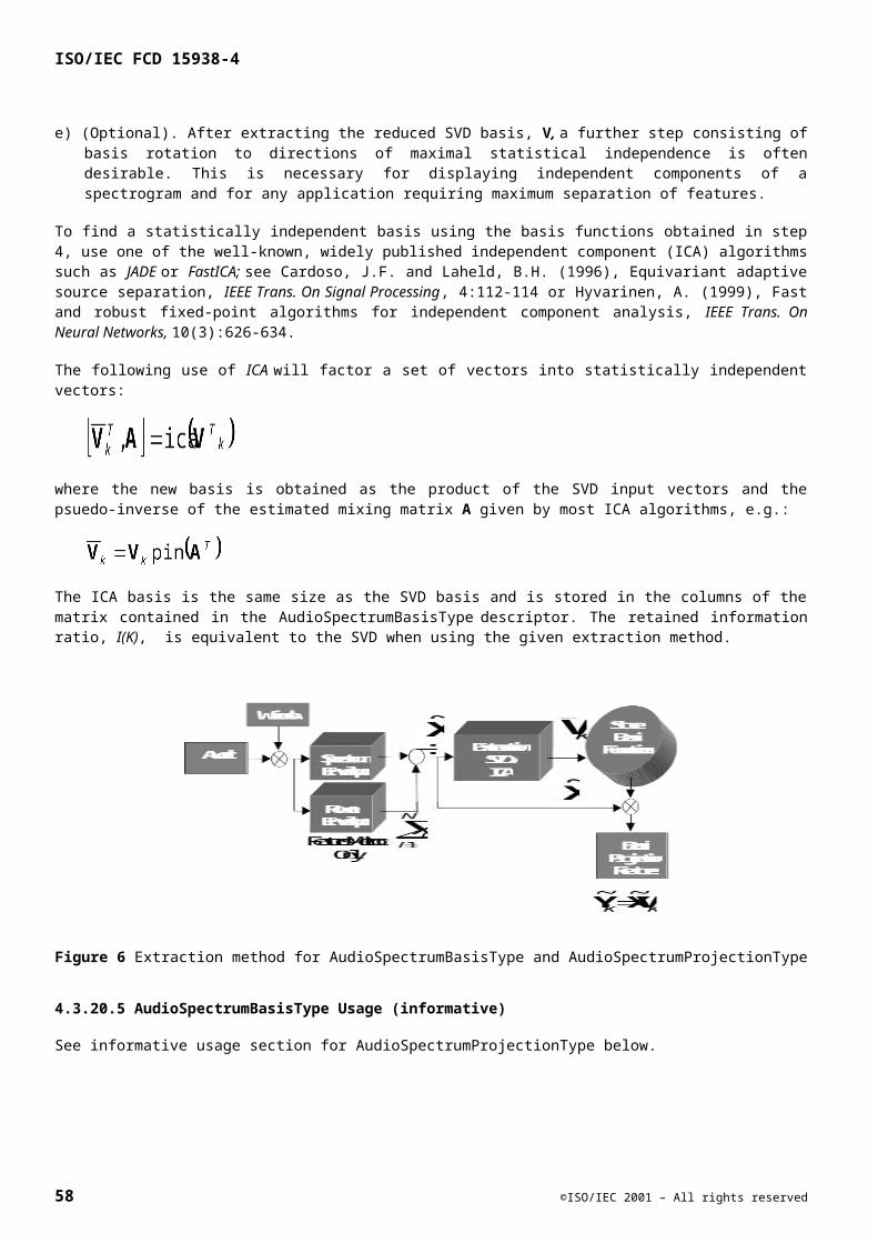
ISO/IEC FCD 15938-4

TimbreType TimbreType

Table 1 Sounds family

A reduced set of descriptors is established in order to describe the timbre perception within each family of sounds. So far, only two families are considered: the sustained, harmonic coherent sounds, and the non-sustained sounds.

For each of these families, a set of TimbreDescriptors is established in order to describe the timbre perception between sounds belonging to the same family. These sets are called the HarmonicInstrumentTimbreType and PercussiveInstrumentTimbreType.

Because some sounds may belong to other Timbre Families, a generic set of Timbre Descriptors is included with all of the TimbreDescriptors of the HarmonicInstrumentTimbreType and PercussiveInstrumentTimbreType.

Target applications are:

Authoring Tools for sound designers or musicians (Music Sample database management) and

Retrieval Tools for producers (“Query by example search” based on perceptual features).

5.2.2 Definitions of Terms

Frame: A Frame is defined as a short period of time of the signal on which the instantaneous analysis if perform. For a signal, noted s(t) (in continuous time noted t), and for an analysis window of type hamming, noted h(t) and of temporal length L, the fth signal frame is defined as

where S is the hop size

Hop size: The hop size defines the temporal distance between two successive analysis.

Running window analysis: A running window analysis is an analysis obtained by mutliplying the signal by a window function which is shifted along time by integer multiple of a parameter called the hop size. For a window function h(t), and a hop size S, the fth shifting of the window is equal to h(t-fS).

Instantaneous values: For the instantaneous values of the Timbre descriptors based on harmonic peaks estimation (IHSC, IHSD, IHSS, IHSV), it corresponds to the results of analysis on a frame level. The values of the global values of the Timbre descriptors based on harmonic peak estimation (HSC, HSD, HSS, HSV) correspond to the average over all frames of the segment of the instantaneous values.

5.2.3 InstrumentTimbreType


The InstrumentTimbreType is a set of TimbreDescriptors established in order to describe the timbre perception among sounds belonging simultaneously to the Harmonic and Percussive sound families.

5.2.3.2 Syntax

   <complexType name="InstrumentTimbreType">


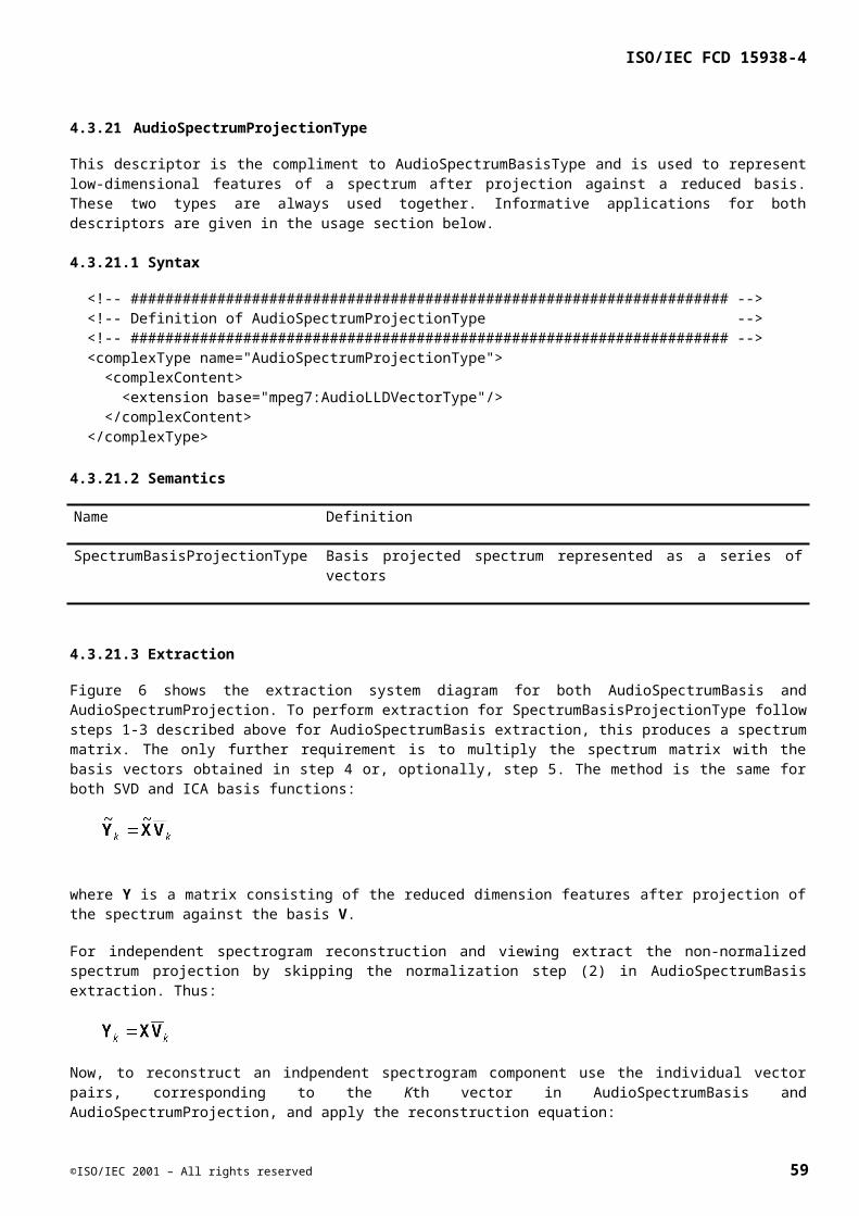
ISO/IEC FCD 15938-4

<complexContent> <extension base="mpeg7:AudioDSType"> <sequence> <element name="LogAttackTime" type="mpeg7:LogAttackTimeType" minOccurs="0"/> <element name="HarmonicSpectralCentroid" type="mpeg7:HarmonicSpectralCentroidType" minOccurs="0"/> <element name="HarmonicSpectralDeviation" type="mpeg7:HarmonicSpectralDeviationType" minOccurs="0"/> <element name="HarmonicSpectralSpread" type="mpeg7:HarmonicSpectralSpreadType" minOccurs="0"/> <element name="HarmonicSpectralVariation" type="mpeg7:HarmonicSpectralVariationType" minOccurs="0"/> <element name="SpectralCentroid" type="mpeg7:SpectralCentroidType" minOccurs="0"/> <element name="TemporalCentroid" type="mpeg7:TemporalCentroidType" minOccurs="0"/> </sequence> </extension> </complexContent> </complexType>

5.2.3.3 Semantics

Name Definition

LogAttackTime (LAT) The LAT is defined as the logarithm (decimal base) of the time the signal starts to the time it reaches its stable part.

Unit: [log sec]

Range: [log(1/sr), determined by the length of the signal]


HarmonicSpectralCentroid (HSC)

The HSC is computed as the average over the sound segment duration of the instantaneous HSC (IHSC) within a running window. The IHSC is computed as the amplitude (linear scale) weighted average of the harmonic peaks of the spectrum.

Unit: [Hz]

Range: [0,sr/2]


HarmonicSpectralDeviation (HSD)

The HSD is computed as the average over the sound segment duration of the instantaneous HSD (IHSD) within a running window. The IHSD is computed as the spectral deviation of amplitude (logarithmic scale) components from a global spectral envelope.

Unit: [-]

Range: [0,1]

HarmonicSpectralSpread (HSS)

The HSS is computed as the average over the sound segment duration of the instantaneous HSS (IHSS) within a running window. The IHSS is computed as the amplitude (linear scale) weighted standard deviation of the


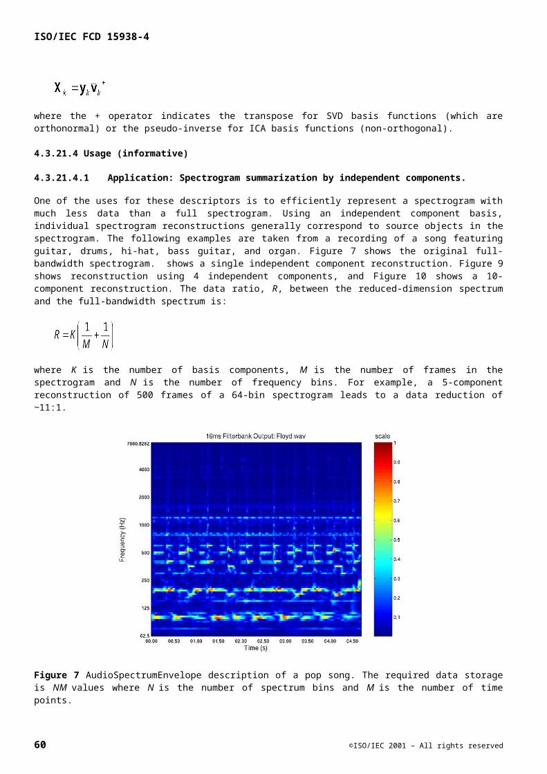
ISO/IEC FCD 15938-4

harmonic peaks of the spectrum, normalized by the IHSC.

Units: [-]

Range: [0,1]

HarmonicSpectralVariation (HSV)

The HSV is defined as the average over the sound segment duration of the instantaneous HSV (IHSV). The IHSV is defined as the normalized correlation between the amplitude (linear scale) of the harmonic peaks of two adjacent frames.

Units: [-]

Range: [0,1]

SpectralCentroid (SC) The SC is computed as the power weighted average of the frequency of the bins in the power spectrum.

Unit: [Hz]

Range: [0,sr/2]


TemporalCentroid (TC) The TC is defined as the time averaged over the energy envelope.

Unit: [sec]


5.2.4 HarmonicInstrumentTimbreType


The HarmonicInstrumentTimbreType is a set of TimbreDescriptors established in order to describe the timbre perception among sounds belonging to Harmonic sound family.

5.2.4.2 Syntax

   <complexType name="HarmonicInstrumentTimbreType"> <complexContent> <extension base="mpeg7:AudioDSType"> <sequence> <element name="LogAttackTime" type="mpeg7:LogAttackTimeType"/> <element name="HarmonicSpectralCentroid" type="mpeg7:HarmonicSpectralCentroidType"/> <element name="HarmonicSpectralDeviation" type="mpeg7:HarmonicSpectralDeviationType"/> <element name="HarmonicSpectralSpread" type="mpeg7:HarmonicSpectralSpreadType"/> <element name="HarmonicSpectralVariation" type="mpeg7:HarmonicSpectralVariationType"/>


ISO/IEC FCD 15938-4

</sequence> </extension> </complexContent> </complexType>

5.2.4.3 Semantics

Name Definition

LogAttackTime (LAT) The LAT is defined as the logarithm (decimal base) of the time the signal starts to the time it reaches its stable part.

Unit: [log sec]

Range: [log(1/sr),determined by the length of the signal]


HarmonicSpectralCentroid (HSC)

The HSC is computed as the average over the sound segment duration of the instantaneous HSC (IHSC) within a running window. The IHSC is computed as the amplitude (linear scale) weighted average of the harmonic peaks of the spectrum.

Unit: [Hz]

Range: [0,sr/2]


HarmonicSpectralDeviation (HSD)

The HSD is computed as the average over the sound segment duration of the instantaneous HSD (IHSD) within a running window. The IHSD is computed as the spectral deviation of amplitude (logarithmic scale) components from a global spectral envelope.

Unit: [-]

Range: [0,1]

HarmonicSpectralSpread (HSS)

The HSS is computed as the average over the sound segment duration of the instantaneous HSS (IHSS) within a running window. The IHSS is computed as the amplitude (linear scale) weighted standard deviation of the harmonic peaks of the spectrum, normalized by the IHSC.

Units: [-]

Range: [0,1]

HarmonicSpectralVariation (HSV)

The HSV is defined as the average over the sound segment duration of the instantaneous HSV (IHSV). The IHSV is defined as the normalized correlation between the amplitude (linear scale) of the harmonic peaks of two adjacent frames.

Units: [-]

Range: [0,1]


ISO/IEC FCD 15938-4

5.2.5 PercussiveInstrumentTimbreType


The PercussiveInstrumentTimbreType is a set of TimbreDescriptors established in order to describe the timbre perception among sounds belonging to Percussive sound family.

5.2.5.2 Syntax

   <complexType name="PercussiveInstrumentTimbreType"> <complexContent> <extension base="mpeg7:AudioDSType"> <sequence> <element name="LogAttackTime" type="mpeg7:LogAttackTimeType"/> <element name="SpectralCentroid" type="mpeg7:SpectralCentroidType"/> <element name="TemporalCentroid" type="mpeg7:TemporalCentroidType"/> </sequence> </extension> </complexContent> </complexType>

5.2.5.3 Semantics

Name Definition

LogAttackTime (LAT)

The LAT is defined as the logarithm (decimal base) of the time the signal starts to the time it reaches its stable part.

Unit: [log sec]

Range: [log(1/sr),determined by the length of the signal]


SpectralCentroid (SC)

The SC is computed as the power weighted average of the frequency of the bins in the power spectrum.

Unit: [Hz]

Range: [0,sr/2]


TemporalCentroid (TC)

The TC is defined as the time averaged over the energy envelope.

Unit: [sec]



ISO/IEC FCD 15938-4

5.2.6 Usage, extraction and examples (informative)

5.2.6.1 Distance measures

Timbre descriptors can be combined in the following suggested way in order to allow a comparison of sounds according to perceptual features:

For sound family 1 one obtains the following expression for the distance:

For sound family 3 one obtains the following expression for the distance:

In both cases, is the difference between the values of the same acoustical parameter for the two sounds considered.

It should be noted that the exact coefficients may be different from one database to another depending on the set of sounds included. The above coefficients are approximations to values derived from a specific database used for experimental verification of the descriptors; they are provided only as an example for informative purposes, and may not be appropriate for arbitrary data sets.

5.2.6.2 Example of InstrumentTimbre

<AudioDS xsi:type="InstrumentTimbreType"> <LogAttackTime> <Scalar>-0.801455</Scalar> </LogAttackTime> <HarmonicSpectralCentroid> <Scalar>1704.46</Scalar> </HarmonicSpectralCentroid> <HarmonicSpectralDeviation> <Scalar>0.00623285</Scalar> </HarmonicSpectralDeviation> <HarmonicSpectralSpread> <Scalar>0.482463</Scalar> </HarmonicSpectralSpread> <HarmonicSpectralVariation> <Scalar>0.950002</Scalar> </HarmonicSpectralVariation> <SpectralCentroid> <Scalar>1781.83</Scalar> </SpectralCentroid> <TemporalCentroid> <Scalar>0.698057</Scalar> </TemporalCentroid> </AudioDS>

5.2.6.3 Example of HarmonicInstrumentTimbre

<AudioDS xsi:type="HarmonicInstrumentTimbreType"> <LogAttackTime> <Scalar>-0.287534</Scalar> </LogAttackTime> <HarmonicSpectralCentroid> <Scalar>1283.934897</Scalar> </HarmonicSpectralCentroid>


ISO/IEC FCD 15938-4

<HarmonicSpectralDeviation> <Scalar>0.004985</Scalar> </HarmonicSpectralDeviation> <HarmonicSpectralSpread> <Scalar>0.509329</Scalar> </HarmonicSpectralSpread> <HarmonicSpectralVariation> <Scalar>0.999198</Scalar> </HarmonicSpectralVariation> </AudioDS>

5.2.6.4 Example of PercussiveInstrumentTimbre

<AudioDS xsi:type="PercussiveInstrumentTimbreType"> <LogAttackTime> <Scalar>-2.060107</Scalar> </LogAttackTime> <SpectralCentroid> <Scalar>2582.49</Scalar> </SpectralCentroid> <TemporalCentroid> <Scalar>0.066983</Scalar> </TemporalCentroid> </AudioDS>


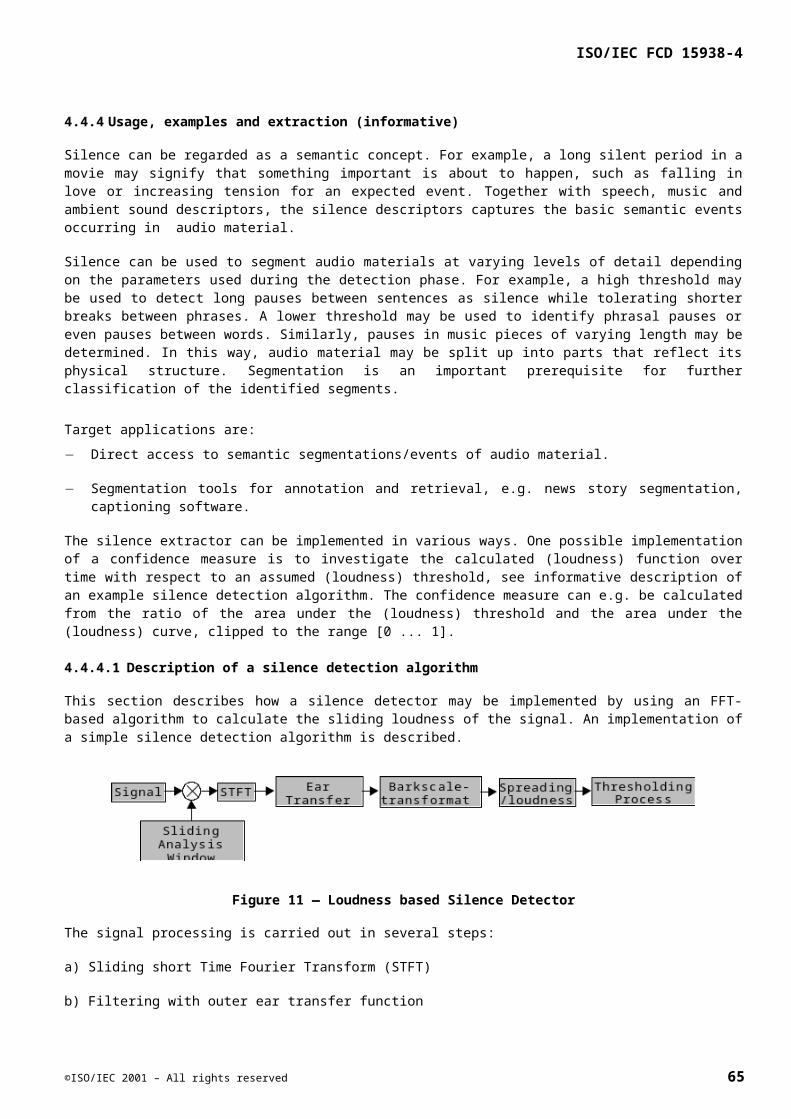
ISO/IEC FCD 15938-4

5.3 Sound Recognition Descriptors and Description Schemes

Note: The Sound Recognition section is not formatted correctly5.3.1 Introduction

The sound recognition descriptors and description schemes consist of tools for indexing audio using probabilistic sound models. The descriptors provide containers for features, probabilistic models and category labels. As such, the descriptors contain both qualitative and quantitative information about sound content.

5.3.2 SoundRecognitionFeatures

This descriptor contains a list of MPEG-7 descriptor elements that are used with probabilistic models for sound recognition. The default descriptors required for sound recognition are AudioPowerType and AudioBasisProjectionType. These descriptors have been shown to perform well for general sound effect recognition. However, for musical instrument recognition the use of harmonic spectral descriptors from the low-level descriptor framework is also required.

Use SoundRecogitionFeaturesType to indicate to a search/retrieval application which low-level descriptors are needed in order to compare a description against a pre-trained model or collection of models. For example, a client-side search and retrieval application must extract a compatible description from client-side sound query data to match against a pre-trained sound model or model collection that resides on a server.

5.3.2.1 Syntax

 

<complexType name="SoundRecognitionFeaturesType"><complexContent>

<extension base="packageType"></extension>

</complexContent></complexType>

5.3.2.2 Semantics

Semantics of the SoundRecognitionFeaturesType:

Name Definition

SoundRecognitionFeaturesType Describes the required low-level tools for matching against a trained model.

ScaleFactors A scaling factor for each element in the SoundRecogntionFeatures package. The scale factors are computed column-wise and each column is divided by its scale factor in order to restrict the range of inputs in each column to –1:1.

Multiply each column by its stored scale factor to invert this mapping and recover the full-range description.


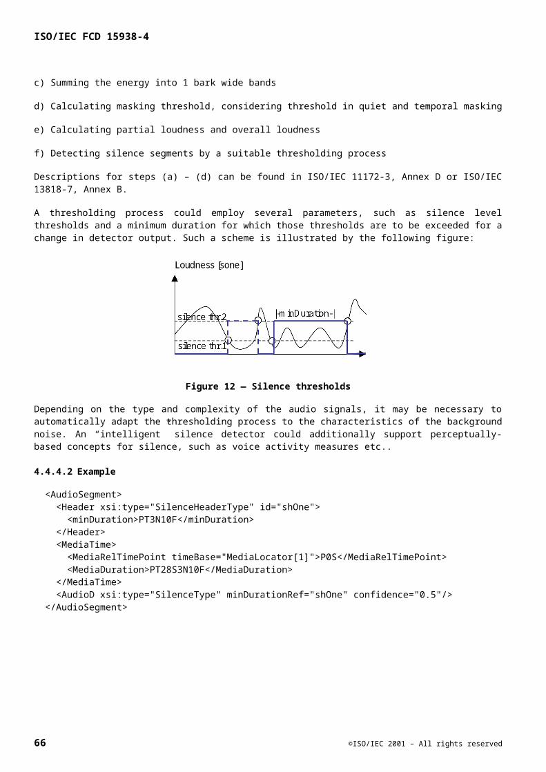
ISO/IEC FCD 15938-4


<SoundRecognitionFeatures name=”DefaultFeatures”><Scheme = “AudioSpectrumProjectionType”><Scheme = “AudioPowerType>

</SoundRecognitionFeatures>

5.3.2.4 Extraction

To ensure that a description is compatible with those stored in a database use the SoundRecognitionFeatures description scheme as follows:

1. Traverse the schemes in the order that they occur in the SoundRecognitionFeatures description. For each scheme, perform the normative or default extraction method as outlined in the Audio Framework section. Schemes are referenced by their MPEG-7 schema names and are typed to avoid conflicts.

In all cases, a series-based extraction shall be used with equivalent sampling periods between descriptors. Compatible sampling shall be performed by uniform use of the hopSize attribute across descriptors, or equivalently, by utilizing a scale-tree scaling ratio that performs re-sampling of descriptors to a uniform frame-rate across descriptors. Frame-rates shall be a positive integer multiple of the default 10ms frame rate.

2. For each feature calculate the scale factors as the maximum absolute value of the series. Scale factors are used to restrict the values to the range –1:1 which corresponds to a sphering of input data:

If the scheme uses a SeriesOfScalars calculate the scale factor for the series and divide each value in the series by that value:

If a SeriesOfVectors, then orient with row-wise time frames, calculate the individual column scale factors and divide

each column by that value:

Store the scale factors each vector of each descriptor (column-wise for Vector descriptors).

3. Concatenate each descriptor column-wise, with frames in the rows, thus forming a combined normalized observation matrix for all descriptors in the SoundRecognitionFeatures package.

For example given a SeriesOfScalars description:

and two SeriesOfVectors descriptions:

then the combined SoundRecognitionFeatures package observation matrix is:


ISO/IEC FCD 15938-4

5.3.3 SoundRecognitionModelType

The following description scheme is used for specifying a probability model of a sound effect class, such as a hidden Markov model or Gaussian mixture model. These models possess states that are used to partition a sound into statistically-significant patterns. The temporal evolution of such states is an important feature for sound recognition and sound matching and may be represented using a matrix of transition probabilities between states. A hidden Markov model describes transitions between states in this manner.

5.3.3.1 Syntax

   <complexType name="SoundModelType">

<complexContent><extension base="mpeg7:AudioDSType">

<element name="ExtractionInformation" type="mpeg7:ExtractionInfoType"/><element name="SoundRecognitionFeatures"

type="mpeg7:SoundRecognitionFeaturesType" use="required"> <element name="ProbabilityModel" type="mpeg7:ProbabilityModelType" use="required"/> <element name="SpectrumBasis" type="mpeg7:AudioSpectrumBasisType" use="required"/> <attribute name="SoundEffectCategoryRef" type="mpeg7:IDREF" use="required"/></complexType>

5.3.3.2 Semantics

Name Definition

SoundRecognitionModelID Unique identifier for the sound effect model

SoundRecognitionCategoryRef Reference to sound category unique identifier

ExtractionInformation Controlled term containing extraction ID and version.

ProbabilityModel A probability model of the sound category, e.g. a HMM

SpectrumBasis Data-derived basis functions for the sound class


<SoundEffectModel id="sfx1.1" SoundEffectCategoryRef="Bark"><ExtractionInformation term="Parameters" scheme="ExtractionParameters"><Label>NumStates=7, NumBasisComponents=5</Label></ExtractionInformation>

<ProbabilityModel xsi:type="ContinuousMarkovModelType" numberStates="7"><Initial dim="7"> 0.04 0.34 0.12 0.04 0.34 0.12 0.00 </Initial><Transitions dim="7 7">0.91 0.02 0.00 0.00 0.05 0.01 0.01 0.01 0.99 0.00 0.00 0.00 0.00 0.00 0.01 0.00 0.92 0.01 0.01 0.06 0.00 0.00 0.00 0.00 0.99 0.01 0.00 0.00


ISO/IEC FCD 15938-4

0.02 0.00 0.00 0.00 0.97 0.00 0.00 0.00 0.00 0.01 0.00 0.00 0.98 0.01 0.02 0.00 0.00 0.00 0.00 0.02 0.96 </Transitions><State><Label>1</Label></State><!—State 1 Observation Distribution -- ><ObservationDistribution xsi:type="GaussianDistributionType"><Mean dim="6">5.11 -9.28 -0.69 -0.79 0.38 0.47 </Mean><Covariance dim="6 6">1.40 -0.12 -1.53 -0.72 0.09 -1.26 -0.12 0.19 0.02 -0.21 0.23 0.17 -1.53 0.02 2.44 1.41 -0.30 1.69 -0.72 -0.21 1.41 2.27 -0.15 1.05 0.09 0.23 -0.30 -0.15 0.80 0.29 -1.26 0.17 1.69 1.05 0.29 2.24 </Covariance><State><Label>2</Label></State><!—Remaining states use same structures-- ><\PobabilityModel>

<AudioSpectrumBasis loEdge="62.5" hiEdge="8000" resolution="1/4 octave"> <Matrix dim="31 5">

0.26 -0.05 0.01 -0.70 0.44 0.34 0.09 0.21 -0.42 -0.05 0.33 0.15 0.24 -0.05 -0.39 0.33 0.15 0.24 -0.05 -0.39 0.27 0.13 0.16 0.24 -0.04 0.27 0.13 0.16 0.24 -0.04 0.23 0.13 0.09 0.27 0.24 0.20 0.13 0.04 0.22 0.40 0.17 0.11 0.01 0.14 0.37

. . .  </Matrix>

</AudioSpectrumBasis>

</SoundEffectModel>

5.3.4 SoundRecognitionStatePathType

This descriptor refers to a finite-state probability model, such as a hidden Markov model (HMM), and describes the dynamic state path of a sound through the model. Sounds may be described by segmenting into model states or by sampling of the state path at regular intervals. In the first case, each segment contains a reference to a state, and the duration of the segment indicates the duration of activation for the state. In the second approach the sound is described by a sampled series of indices that reference the model states. Sound categories with long state durations are efficiently described using the one-segment, one-state approach. Sounds with short state durations are more efficiently described using the sampled series of state indices.

5.3.4.1 Syntax



<complexType name="SoundModelStatePathType"> <complexContent> <extension base="mpeg7:AudioSampledType">


ISO/IEC FCD 15938-4

<element name="SoundEffectModelRef" type="mpeg7:IDREF" use="required"/> <sequence minOccurs="0">

<element name="StateRef" type="mpeg7:IDREF" use="required"/> </sequence> <element name="StatePath" type="mpeg7:SeriesOfScalarType" minOccurs="0"/> </extension> </complexContent> </complexType>

5.3.4.2 Semantics

Name Definition

SoundRecognitionModelRef Reference to a sound effect probability model

StateRef Reference to a unique state identifier

StatePath Regularly sampled series of ordinal state indices

5.3.5 SoundModelStateHistogramType

This descriptor provides a method for describing a sound in terms of a state occupancy histogram derived from a finite-state model. The purpose of the descriptor is to provide a means to compare sounds by the distribution of model states from a SoundModelType description.

5.3.5.1 Syntax



<complexType name="SoundModelStateHistogramType"> <complexContent> <extension base="mpeg7:AudioDType">

<element name="SoundEffectModelRef" type="mpeg7:IDREF" use="required"/> <sequence minOccurs="1"> <element name="StateRef" type="mpeg7:IDREF" use="required"/> <element name="Frequency" type="mpeg7:float" use=required" /> </sequence> </extension> </complexContent> </complexType>

5.3.5.2 Semantics

Name Definition

SoundRecognitionModelRef Reference to a SoundModelType description scheme

StateRef Reference to a unique state identifier

Frequency Relative frequency of state compared to all other states


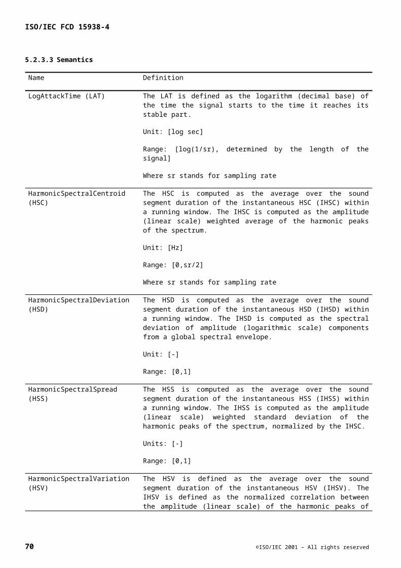
ISO/IEC FCD 15938-4

Name Definition

in the referenced SoundModelType.

The similarity metric for this descriptor is the sum of squared errors between state frequencies.

5.3.6 SoundClassifierType

This description scheme is used for grouping a number of probability models into a sound classifier. For example, a hierarchical classifier can be built using SoundModelType description schemes that recognizes broad sound classes, such as animals:noises, at the root nodes and finer classes, such as dogs:barks and birds:cukoos, at the leaf nodes.

5.3.6.1 Syntax

   <complexType name="SoundClassifierType">

<complexContent><extension base="mpeg7:AudioDSType">

<sequence maxOccurs="unbounded"> <element name="SoundModelRef" type="mpeg7:IDREF"/> </sequence>

</extension></complexContent>

</complexType>

5.3.6.2 Semantics

Name Definition

SoundModelRef Unique identifier for SoundModelType schemes

5.3.7 Usage, extraction and examples

5.3.7.1 Extraction

The figure below illustrates an automatic extraction system for describing sound effects. A statistical basis for each class of sound is extracted and is used to project each sound into a classification space. The sounds are first converted to a spectrum representation and then projected against the extracted basis to yield reduced dimension features.

The second stage is to train a probability model, such as a hidden Markov model (HMM), using basis-derived features from a corpus of sound examples. The HMM is trained using the well-known Baum-Welch algorithm. The resulting HMM model and the statistical basis functions are stored on disk in DDL format. Finally, each sound is passed through the Viterbi algorithm giving both a best-fit model and the state path through the model during the course of the sound. This completes the sound description.


ISO/IEC FCD 15938-4

Figure 13 — Hidden Markov model extraction and SoundRecognitionStatePath description

5.3.7.2 Application Example 1: Description-based Query by Example

A query-by-example system is shown in the figure below. A sound query is presented to the system using the SoundRecognitionStatePath description scheme format. The system reads the query and populates data structures with the description information. This sound description information is then compared to descriptions taken from a sound database stored on disk. A matching algorithm is applied, and a sorted result list consisting of N closest matches is returned.

Figure 14 — Query-by-example from a pre-computed description

5.3.7.3 Application Example 2: Media-based query by example

The system shown below implements a more sophisticated version of the query-by-example application using an audio query. In this case, the first stage of extraction must be applied, namely spectrogram and envelope computation followed by projection against a stored set of basis functions for each model in the classifier. The resulting dimension-reduced features are passed to the classifier and the HMM with the maximum likelihood score for the given features is selected. A model reference and a state path are recorded and the results are matched against a pre-computed database as in the first example.


ISO/IEC FCD 15938-4

Figure 15 — Media-based query-by-example

5.3.8 SoundCategoryType

This descriptor provides a mechanism for constructing taxonomies of sound categories. Categories can be used to index an audio signal with a suitable semantic label, for example violin, gun shot or applause.

5.3.8.1 Syntax

<complexType name="SoundCategoryType"> <complexContent> <extension base="mpeg7:ControlledTermType"> </extension> </complexContent></complexType>

5.3.8.2 Semantics

Name Definition

SoundID Unique identifier for sound category


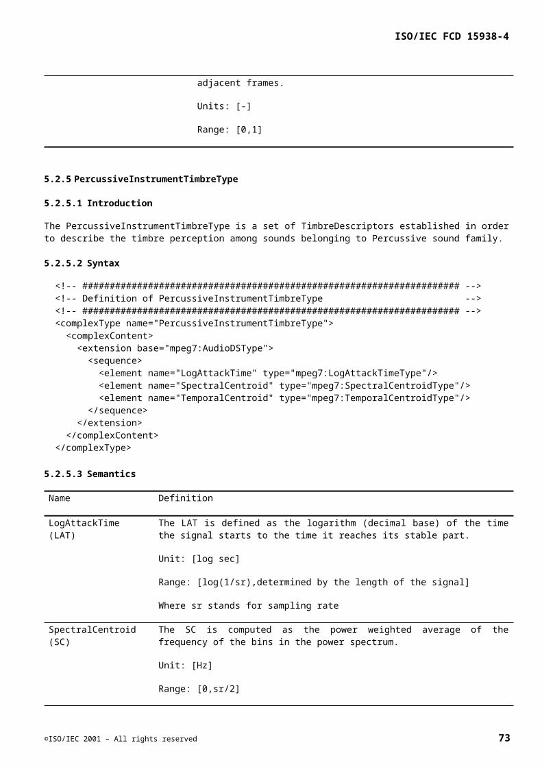
ISO/IEC FCD 15938-4


Sound categories extend the controlled term description scheme defined in the MDS part of the standard. The following example code shows how to instantiate the SoundCategory description scheme for the category “Dogs” using the MPEG-7 description definition language (DDL):

<SoundCategory term=”1” scheme=”DOGS”> <Label>Dogs</Label> <TermRelation term=”1.1” scheme=”DOGS”> <Label>Bark</Label> <TermRelation term=”1.2” scheme=”DOGS” type=”UF”> <Label>Woof</Label> </TermRelation> </TermRelation> <TermRelation term=”1.3” scheme=”DOGS”> <Label>Howl</Label> </TermRelation></SoundCategory>

The term and scheme attributes together provide unique identifiers that are used for referencing categories and taxonomies from other description schemes such as probabilistic models. The Label descriptor gives a meaningful semantic label for each category and the TermRelation descriptor describes relationships amongst terms in the taxonomy.

Categories may be combined into classification schemes to make a richer taxonomy; for example, “Barks” is a sub-category of “Dogs” which is a sub-category of “Pets”; as is the category “Cats”. The following is an example of a simple classification scheme for “Pets” containing two categories: “Dogs” and “Cats”.

Figure 2. Combining categories into a larger taxonomy.

To implement this classification scheme by extending the previously defined scheme, a second scheme, named “CATS”, is instantiated as follows:

<SoundCategory term=”2” scheme=”CATS”> <Label>Cats</Label> <TermRelation term=”2.1 scheme=”CATS”> <Label>Meow</Label> </TermRelation> <TermRelation term=”2.2” scheme=”CATS”> <Label>Purr</Label> </TermRelation></SoundCategory>

Now to combine these categories, a ClassificationScheme, called “PETS”, is instantiated that references the previously defined schemes:


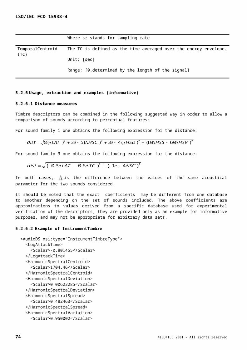
ISO/IEC FCD 15938-4

<ClassificationScheme term=”0” scheme=”PETS”> <Label>Pets</Label> <ClassificationSchemeRef scheme=”DOGS”/> <ClassificationSchemeRef scheme=”CATS”/></ClassificationScheme>

Now, the classifications scheme called “PETS” consists of all the category components of “DOGS” and “CATS” with the additional category “Pets” as the root. Whilst building a taxonomy may be sufficient for some indexing applications, it is just the first step toward the goal of automatic sound effects classification. The following sections outline quantitative descriptors for classification and indexing. A non-normative list of common-usage sound effect categories is shown in the table below; these examples consist of two hierarchical levels.

The following table needs to be instantiated using the ControlledTerm DS.

Table 2 — Sound effect category examples

AIRPLANES:AIRPORT AIRPLANES:FIGHTERS AIRPLANES:HELICOPTERS

AIRPLANES:JETS ANIMALS:APES ANIMALS:BATS

ANIMALS:CAMELS ANIMALS:CATS ANIMALS:CRICKETS

ANIMALS:DOGS ANIMALS:FARM ANIMALS:HORSES

ANIMALS:INSECTS ANIMALS:REPTILES ANIMALS:WILD

AUTOMOBILES:BRAKES AUTOMOBILES:CAR AUTOMOBILES:CARWASH

AUTOMOBILES:CRASH AUTOMOBILES:DOORS AUTOMOBILES:DRIVING

AUTOMOBILES:EXT AUTOMOBILES:GENERAL AUTOMOBILES:HORNS

AUTOMOBILES:IDLE AUTOMOBILES:INT AUTOMOBILES:SEATBELTS

AUTOMOBILES:SKIDS AUTOMOBILES:WINDOWS BALLS:BOUNCE:

BELLS: BIRDS: BIRDS:CROWS

BIRDS:EXT BIRDS:FARM BIRDS:FINCHES

BIRDS:FLYCATCHERS BIRDS:GAME BIRDS:PETS

BIRDS:PIGEONS BIRDS:PREDATORS BIRDS:SEAGULLS

BIRDS:SONGBIRDS BIRDS:TROPICAL BIRDS:WATER

BIRDS:WOODPECKERS BOATS:BOW BOATS:FERRYBOATS

BOATS:HORNS BOATS:MILITARY BOATS:MOTORBOATS

BOATS:ONBOARD BOATS:SAILBOATS BOATS:SUBMARINES

CARTOONS:BUBBLES CARTOONS:EXPLOSIONS CARTOONS:TWANGS

CARTOONS:WHISTLES COMMUNICATIONS:COMPUTER

COMMUNICATIONS:RADIO

COMMUNICATION:TELEPHONE

CRASHES:GLASS CRASHES:METAL

CRASHES:WOOD ELEMENTS:AIR ELEMENTS:EARTH

ELEMENTS:ELECTRICITY ELEMENTS:FIRE ELEMENTS:GAS

ELEMENTS:ICE ELEMENTS:STORMS ELEMENTS:WATER

ELEMENTS:WIND EMERGENCY:SIRENS FANTASY:HORROR

FANTASY:MAGIC FANTASY:SCI FANTASY:SYNTH


ISO/IEC FCD 15938-4

FOLEY:CLOTH FOLEY:CONCRETE FOLEY:DROPPING

FOLEY:FOLIAGE FOLEY:GLASS FOLEY:GRABBING

FOLEY:HARD FOLEY:HITTING FOLEY:KEYS

FOLEY:LEATHER FOLEY:LINOLEUM FOLEY:LOCKS

FOLEY:METAL FOLEY:PAPER FOLEY:POPPING

FOLEY:PUNCHING FOLEY:RATTLING FOLEY:RATTLING/SHAKING

FOLEY:SLAPPING FOLEY:SQUEAKING FOLEY:WALKING

FOLEY:WARFARE FOLEY:WOOD HOUSEHOLD:AIR

HOUSEHOLD:APPLIANCES HOUSEHOLD:BATHROOM HOUSEHOLD:CLOCKS

HOUSEHOLD:FIXING HOUSEHOLD:GARDENING HOUSEHOLD:HOUSECLEANING

HOUSEHOLD:KITCHEN HOUSEHOLD:TOYS HUMAN:APPLAUSE

HUMAN:AUDIENCE HUMAN:BABIES HUMAN:BODY

HUMAN:CHILDREN HUMAN:CROWDS HUMAN:FEMALE

HUMAN:FOOTSTEPS HUMAN:MALE HUMAN:TEENS

HUMAN:VOCALS INDUSTRY:CONSTRUCTION INDUSTRY:FACTORY

INDUSTRY:HAND INDUSTRY:LOGGING INDUSTRY:MACHINE

INDUSTRY:OFFICE INDUSTRY:POWER INDUSTRY:PRINTING

INDUSTRY:PUMPS SIGNALS:ALARMS SIGNALS:BELLS

SPORTS:BOXING SPORTS:CRICKET SPORTS:FENCING

SPORTS:RACING SPORTS:SOCCER SPORTS:SWIMMING

TRAINS:COMMUTER TRAINS:DIESEL TRAINS:ELECTRIC

TRAINS:FREIGHT TRAINS:HORNS TRAINS:INT

TRAINS:STATION TRAINS:STEAM TRAINS:SUBWAY

TRAINS:VARIOUS TRAINS:WHISTLES VEHICLES:BICYCLES

VEHICLES:BUSES VEHICLES:MILITARY VEHICLES:MOTORCYCLES

VEHICLES:STREET VEHICLES:TRUCKS WARFARE:AUTOMATIC

WARFARE:BATTLE WARFARE:BOMBS WARFARE:EXPLOSIONS

WARFARE:FUTURISTIC WARFARE:GUN WARFARE:MILITARY

WARFARE:RICOCHETS WARFARE:RIFLES WARFARE:SMALL

WHISTLES: WIND: WOODWINDS:

WRESTLING: WRESTLING:ANNOUNCERS: WRITING:

WRITING:CHALK: WRITING:FELT:TIPS:PENS: WRITING:PENCILS:

WRITING:PENS: XMAS: XYLOPHONE:

XYLOPHONE:GLISS:DOWN: XYLOPHONES: XYLOPHONES:UP&DOWN:

XYLOPHONES:UP: YAWNS: YEEHAA:

YELLING: YELLOWHAMMER: YELLS:

YELPING: YODELLING: YODELLING:MALE:

YUKS: ZAPS: ZIMMER:FRAMES:


ISO/IEC FCD 15938-4

ZIPPOS: ZIPS: ZIPS:DOWN:

ZIPS:UP: ZIPS:UP:DOWN: ZOOS:


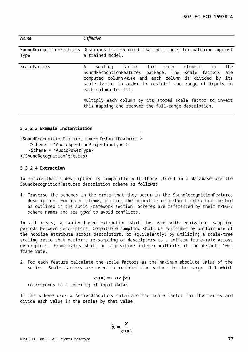
ISO/IEC FCD 15938-4

5.4 Spoken Content

5.4.1 Introduction

The Spoken Content DSs are a representation of the output of Automatic Speech Recognition (ASR). The SpokenContentLatticeType represents the actual decoding produced by an ASR engine, whereas the SpokenContentHeaderType contains information about the recogniser itself and the people (or "Speakers") being recognised.

The Spoken Content DSs consist of combined word and phone lattices for each speaker in an audio stream. By combining the lattices, the problem of out-of-vocabulary (OOV) words is greatly alleviated and retrieval may still be carried out when the original decoding was in error. The DSs can be used for two broad classes of retrieval scenario: indexing into and retrieval of an audio stream, and indexing of multimedia objects annotated with speech. The DSs attempt to be memory efficient while also retaining the flexibility to accommodate currently unforeseen uses.

In the context of the Spoken Content DSs, the word “phone” is used to refer to the sub-word units used in automatic speech recognition.

Example applications include

a) Recall of audio/video data by memorable spoken events. An example would be a film or video recording where a character or person spoke a particular word or sequence of words. The source media would be known, and the query would return a position in the media.

b) Spoken Document Retrieval. In this case, there is a database consisting of separate spoken documents. The result of the query is the relevant documents, and optionally the position in those documents of the matched speech.

c) Annotated Media Retrieval. This is similar to spoken document retrieval, but the spoken part of the media would generally be quite short (a few seconds). The result of the query is the media which is annotated with speech, and not the speech itself. An example is a photograph retrieved using a spoken annotation.

5.4.2 SpokenContentHeaderType

5.4.2.1 Syntax

   <complexType name="SpokenContentHeaderType"> <complexContent> <extension base="mpeg7:HeaderType"> <sequence> <choice maxOccurs="unbounded">   <element name="WordLexicon" type="mpeg7:WordLexiconType"/> <element name="PhoneLexicon" type="mpeg7:PhoneLexiconType"/> </choice> <element name="ConfusionStatistics" type="mpeg7:ConfusionStatisticsType" minOccurs="0" maxOccurs="unbounded"/> <element name="DescriptionMetadata" type="mpeg7:DescriptionMetadataType" minOccurs="0"/>  <element name="SpeakerInfo" type="mpeg7:SpeakerInfoType" maxOccurs="unbounded"/>


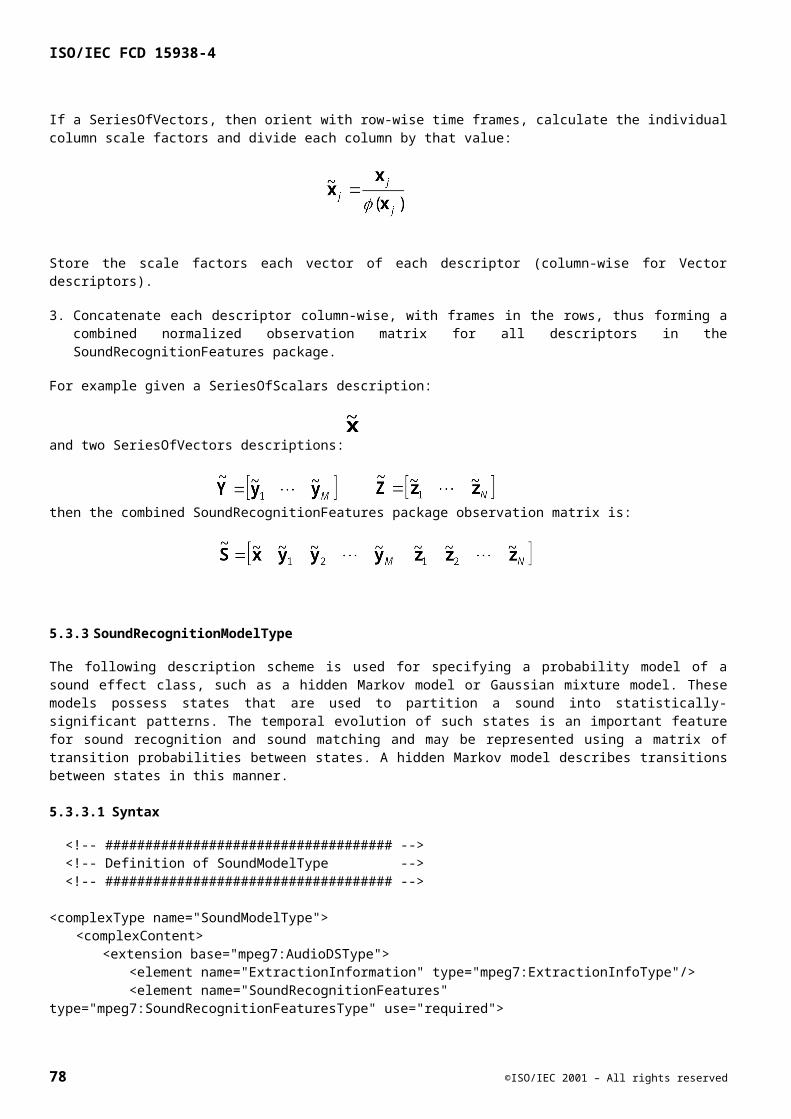
ISO/IEC FCD 15938-4

</sequence> </extension> </complexContent> </complexType>

5.4.2.2 Semantics

Name Definition

SpokenContentHeaderType Header information for Spoken Content in a description.

SpeakerInfo Information about the speakers, ie. the people speaking in the audio.

WordLexicon A list of words. For a complete description, see the definition of WordLexiconType.

PhoneLexicon A list of phones. For a complete description, see the definition of PhoneLexiconType.

ConfusionInfo A data structure of phone confusion information. Although separate, the confusion information must map onto the phone lexicon with which it is associated via the SpeakerInfo.

5.4.3 SpeakerInfoType

5.4.3.1 Syntax

   <complexType name="SpeakerInfoType"> <complexContent> <extension base="mpeg7:HeaderType"> <sequence> <element name="SpokenLanguage" type="language"/> <element name="Person" type="mpeg7:PersonType" minOccurs="0"/> <element name="WordIndex" minOccurs="0"> <complexType> <sequence> <element name="WordIndexEntry" maxOccurs="unbounded"> <complexType> <sequence> <element name="IndexEntry" type="mpeg7:SpokenContentIndexEntryType" maxOccurs="unbounded"/> </sequence> <attribute name="key" use="required"> <simpleType> <list itemType="mpeg7:WordType"/> </simpleType> </attribute> </complexType> </element> </sequence> <attribute name="defaultLattice" type="uriReference" use="required"/>


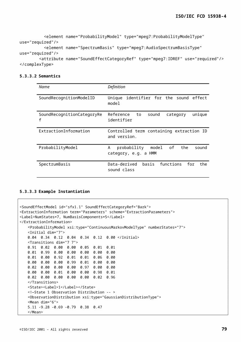
ISO/IEC FCD 15938-4

</complexType> </element> <element name="PhoneIndex" minOccurs="0"> <complexType> <sequence> <element name="PhoneIndexEntry" maxOccurs="unbounded"> <complexType> <sequence> <element name="IndexEntry" type="mpeg7:SpokenContentIndexEntryType" maxOccurs="unbounded"/> </sequence> <attribute name="key" use="required"> <simpleType> <list itemType="mpeg7:PhoneType"/> </simpleType> </attribute> </complexType> </element> </sequence> <attribute name="defaultLattice" type="uriReference" use="required"/> </complexType> </element> </sequence> <attribute name="phoneLexiconRef" type="uriReference"/> <attribute name="wordLexiconRef" type="uriReference"/> <attribute name="confusionStatisticsRef" type="uriReference"/> <attribute name="descriptionMetadataRef" type="uriReference"/> <attribute name="provenance" use="required"> <simpleType> <restriction base="NMTOKEN"> <enumeration value="unknown"/> <enumeration value="ASR"/> <enumeration value="manual"/> <enumeration value="keyword"/> <enumeration value="parsing"/> </restriction> </simpleType> </attribute> </extension> </complexContent> </complexType>

5.4.3.2 Semantics

Name Definition

SpeakerInfoType Speaker information for a speaker in a Spoken Content description scheme.

This is actually more of a collection point for information about a lattice. It contains a "Person DS" element representing the person who is speaking, but also contains indexes and references to confusion information and lexicons.

SpokenLanguage The language which the speaker is speaking. This is distinct from the language in which the description is written. It is implicitly assumed that the word and phone lexicons are applicable for the spoken language.

DescriptionMetadata Information about the extraction process, and any settings that may be pertinent to


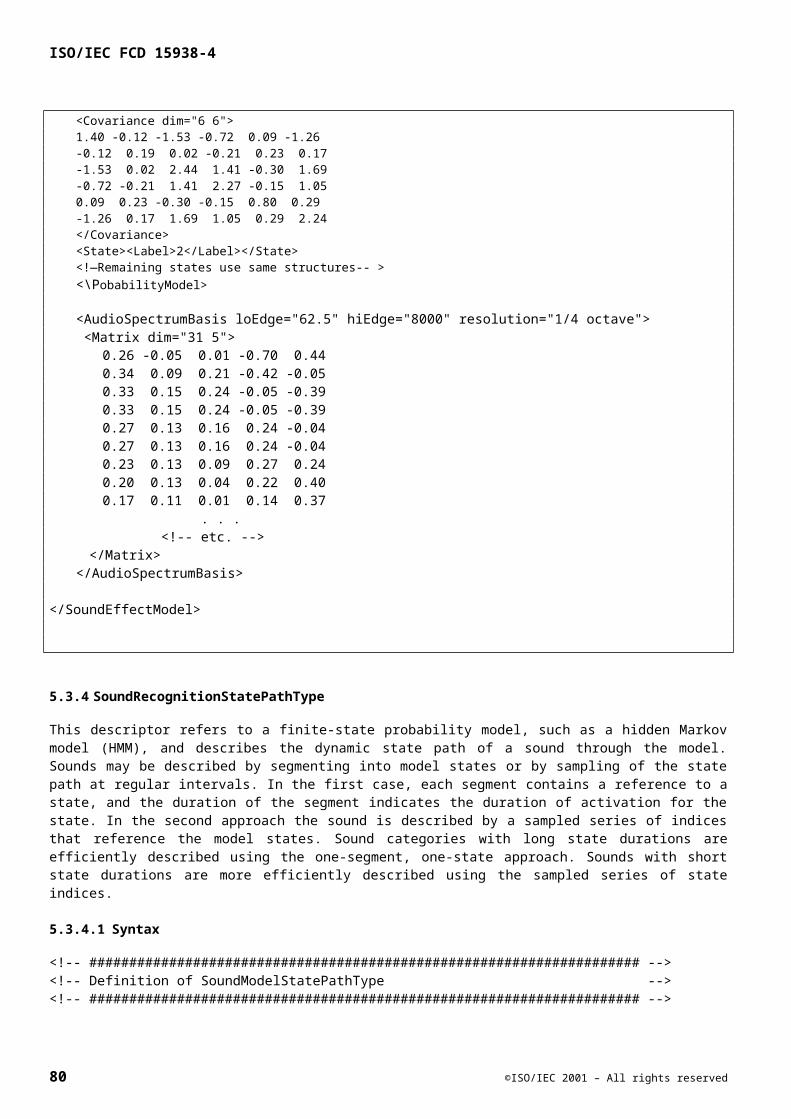
ISO/IEC FCD 15938-4

Name Definition

the retrieval process. For more information, see part 5.

Person An individual person who is speaking. This field is optional in that the Person may be unknown, but can be used to store the name of the speaker.

WordIndex An Index for the words in the lattice. The index consists of a list of words or word “n-grams” (sequences of consecutive words), together with pointers to where each word or word n-gram occurs in the lattices. The design is such that each speaker has a single word index.

WordIndexEntry An entry in the word index

IndexEntry A lattice/block/node triple determining a point in a lattice where the key occurs. This has the same meaning in both the word and phone indexes

key The index key, which is an n-gram of words (in the word index) or phones (in the phone index). A single word corresponds to a basic keyword index. In the phone index, a phone triple (3-gram) is likely to be the most useful form, but any size n-gram is allowed

PhoneIndex An Index for the phones in the lattice. The index consists of a list of phones or phone “n-grams” (sequences of consecutive phones), together with pointers to where each phone or phone n-gram occurs in the lattices. The design is such that each speaker has a single phone index.

PhoneIndexEntry An entry in the phone index

defaultLattice The default lattice for the lattice entries in the index. This has the same meaning in both the word and phone indexes.

phoneLexiconRef A reference to the phone lexicon used by this speaker. Many speakers are likely to share the same phone lexicon

wordLexiconRef A reference to the word lexicon used by this speaker. Many speakers are likely to share the same word lexicon

confusionStatisticsRef A reference to the confusion statistics for the phone lexicon. This attribute is not required, but if used must tally with the phone lexicon, that is, the lexicon provides the labels for the confusion information

descriptionMetadataRef A reference to a DescriptionMetadataType for this speaker. It could be the same as that used for other speakers, or may be different

provenance The provenance of this decoding.

Unknown: The provenance is unknown

ASR: The decoding came from an Automatic Speech Recognition system. This is the most likely value.

Manual: The lattice is manually derived rather than automatic

Keyword: The lattice consists only of keywords rather than full text. This means that either the ASR was used in word spotting mode (treating the majority of the speech as garbage), or that a manual annotation only chose selected words. Each word should appear as it was spoken in the data,


ISO/IEC FCD 15938-4

Name Definition

subject only to ASR errors.

Parsing: The lattice is the result of a higher level parse, perhaps to discern topic or a summary. In this case, a word in the lattice might not correspond directly to words spoken in the data.

5.4.4 SpokenContentIndexEntryType

5.4.4.1 Syntax

   <complexType name="SpokenContentIndexEntryType"> <attribute name="node" type="mpeg7:SpokenContentNodeCountType" use="required"/> <attribute name="block" type="mpeg7:SpokenContentBlockCountType" use="required"/> <attribute name="lattice" type="uriReference" use="optional"/> </complexType>

5.4.4.2 Semantics

Name Definition

SpokenContentIndexEntryType The format of an entry in the word or phone index. This is a node/block/lattice triple

node The number of the node at which the index key begins in a particular block

block The number of the block containing the above node

lattice The ID of the lattice containing the above node and block. If omitted, the defaultLattice attribute is used from the index

5.4.5 ConfusionStatisticsType

5.4.5.1 Syntax

   <complexType name="ConfusionStatisticsType"> <complexContent> <extension base="mpeg7:HeaderType"> <sequence> <element name="InsertionCount" type="mpeg7:integerVector"/> <element name="DeletionCount" type="mpeg7:integerVector"/> <element name="SubstitutionCount" type="mpeg7:IntegerMatrixType"/> </sequence> <attribute name="numDimensions" type="positiveInteger" use="required"/>


ISO/IEC FCD 15938-4

</extension> </complexContent> </complexType>

5.4.5.2 Semantics

Confusion statistics characterise a particular ASR engine, possibly in the context of a particular speaker, and are calculated using a sequence of speech for which two "decodings" are available:

a) A canonical "decoding" reflecting the actual pronunciations of the words spoken. This is referred to as sequence A.

b) A real decoding from the ASR engine, of the same form as sequence A, but incorporating corruption characterised as insertion, deletion and substitution of phones. This is referred to as sequence B.

A (dynamic programming) string alignment between the two sequences yields the confusion statistics.

If confusion statistics are provided in a description, then a corresponding PhoneLexicon must also be provided.The correspondence between indices of the confusion is determined by assigning each phone in the phone lexicon a number based on the order of appearance in the phone lexicon. The first phone appearing in the phone lexicon is assigned an index value of one, the second phone an index of two, and so on, continuing to assign increasing sequential numbers to phones in the order that they appear in the phone lexicon.

Name Definition

numDimensions The dimensionality of the vectors and matrix in the ConfusionStatisticsType. This number must correspond to the size of the PhoneLexiconType to which the data applies.

InsertionCount A vector (of length numDimensions) of counts, being the number of times each phone was inserted in sequence B.

DeletionCount A vector (of length numDimensions) of counts, being the number of times each phone was deleted in sequence B.

SubstitutionCount A square matrix (dimension numDimensions) of counts, being the number of times each phone in sequence B was substituted in place of each phone in sequence A. The leading diagonal represents a phone being substituted for itself, i.e., a correct decoding.

Each row corresponds to a and each column to a , that is, each column represents a canonical phone and each row represents a decoded phone.

5.4.5.3 Usage of ConfusionStatistics (Informative)

Although the confusion statistics are stored as pure counts, their use is more likely to be as probabilities. There are many different ways to calculate such probabilities using Bayesian or maximum entropy techniques. A simple example is presented which is based upon maximum likelihood.

Represent the counts in the ConfusionStatisticsType as follows:

Substitutions: is the number of times that phone in sequence B was substituted for phone in sequence A.


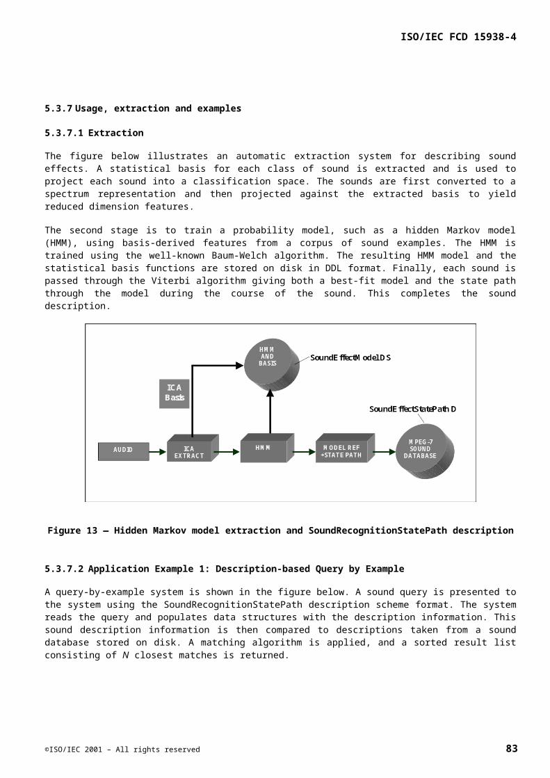
ISO/IEC FCD 15938-4

Insertions: is the number of times that phone was inserted in sequence B when there was nothing in sequence A at that point.

Deletions: is the number of times that phone in sequence A was deleted in sequence B.

The following numbers can easily be calculated:

is the number of times that phone occurs in sequence A.

is the total number of insertions, that is, the number of times any phone appeared in sequence B where there was nothing in sequence A at that point.

Assume also that sequence A is phones in length, and sequence B is phones in length.

The following probabilities can now be calculated:

The unconditional probability of a phone, , being inserted: .

The probability of a phone, , being inserted, given an insertion took place:

The probability of phone, , being inserted: .

The probability of confusing phone as phone : .

5.4.6 SpokenContentBlockCountType and SpokenContentNodeCountType

5.4.6.1 Syntax

     <simpleType name="SpokenContentBlockCountType"> <restriction base="mpeg7:unsigned16"/> </simpleType> <simpleType name="SpokenContentNodeCountType"> <restriction base="mpeg7:unsigned16"/> </simpleType>

5.4.6.2 Semantics

Name Definition

SpokenContentBlockCountType A type definition defining the number of blocks that can exist in a lattice. This is a 16 bit field giving 65536 blocks

SpokenContentNodeCountType As above, but for the number of nodes in a block. Again, 65536.


ISO/IEC FCD 15938-4

5.4.7 WordType and PhoneType

5.4.7.1 Syntax

    <simpleType name="WordType"> <restriction base="string"/> </simpleType> <simpleType name="PhoneType"> <restriction base="string"/> </simpleType>

5.4.7.2 Semantics

Name Definition

WordType A type definition defining what a word is. In XML, this is a string. The WordType must not contain whitespace characters as this precludes the use of word N-Grams as index keys.

PhoneType As above, but for phones. Again, just a string The PhoneType must not contain whitespace characters as this precludes the use of phone N-Grams as index keys.

5.4.8 LexiconType

5.4.8.1 Syntax

   <complexType name="LexiconType" abstract="true"> <complexContent> <extension base="mpeg7:HeaderType"> <attribute name="numOriginalEntries" type="positiveInteger"/> </extension> </complexContent> </complexType>

5.4.8.2 Semantics

Name Definition

LexiconType An abstract base type representing a lexicon. A lexicon is a list of tokens. The tokens should be added by extension of this type.

numOriginalEntries The original size of the lexicon. In the case of a word lexicon, this should be the number of words originally known to the ASR system, whereas the actual size of the lexicon need only consist of those words decoded in the lattice


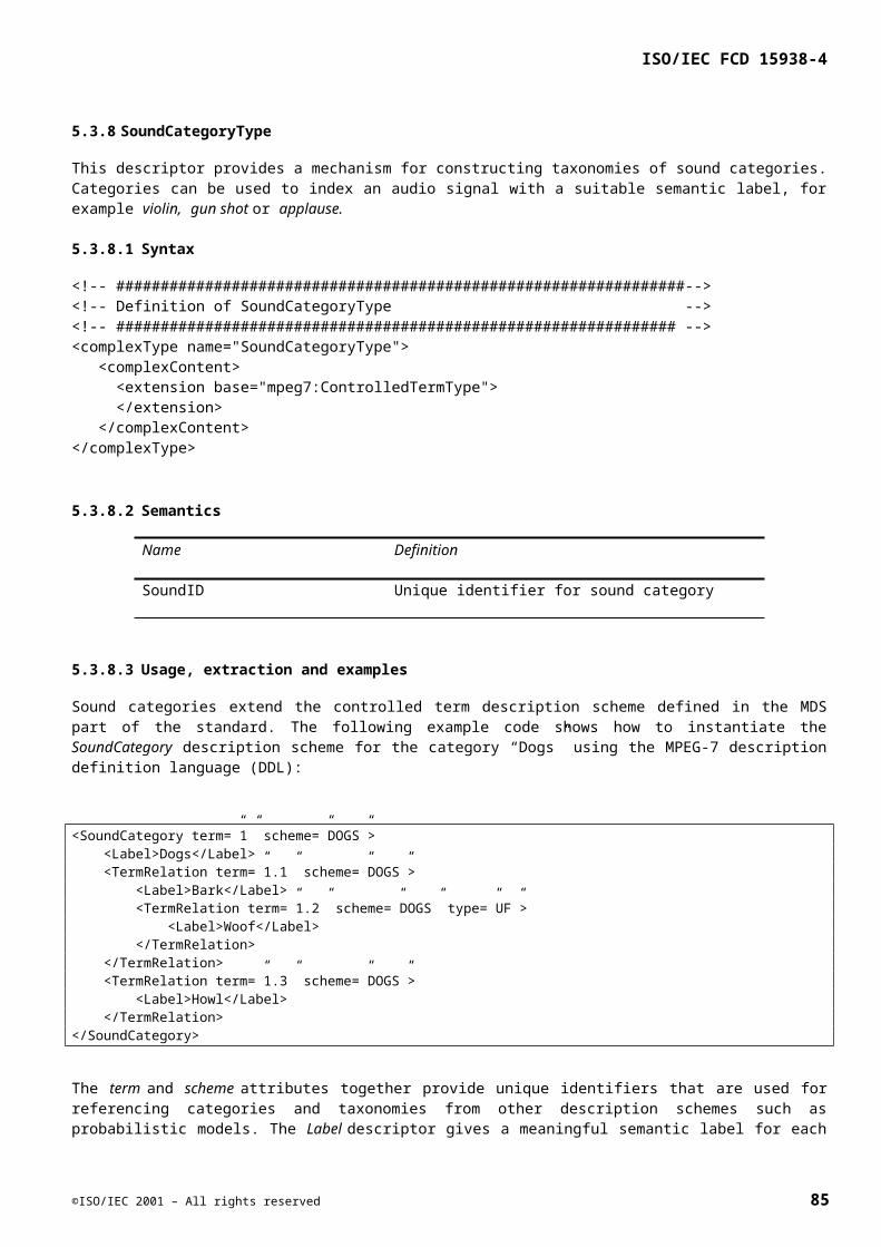
ISO/IEC FCD 15938-4

5.4.9 WordLexiconType

5.4.9.1 Syntax

   <complexType name="WordLexiconType"> <complexContent> <extension base="mpeg7:LexiconType"> <sequence> <element name="Token" type="mpeg7:WordType" maxOccurs="unbounded"/> </sequence> </extension> </complexContent> </complexType>

5.4.9.2 Semantics

Name Definition

WordLexiconType A lexicon of words. Each entry represents one orthographic transcription – i.e. a spelling — of a word. Therefore, the lexicon is not a phonetic (pronunciation) dictionary.

Token An entry in the lexicon

5.4.10 phoneticAlphabetType

5.4.10.1 Syntax

   <simpleType name="phoneticAlphabetType">    <restriction base="NMTOKEN"> <enumeration value="SAMPA"/> <enumeration value="IPASymbol"/> <enumeration value="IPANumber"/> <enumeration value="other"/> </restriction> </simpleType>

5.4.10.2 Semantics

Name Definition

phoneticAlphabetType The name of the phonetic alphabet:

SAMPA. The speech assessment methods phonetic alphabet. This class also


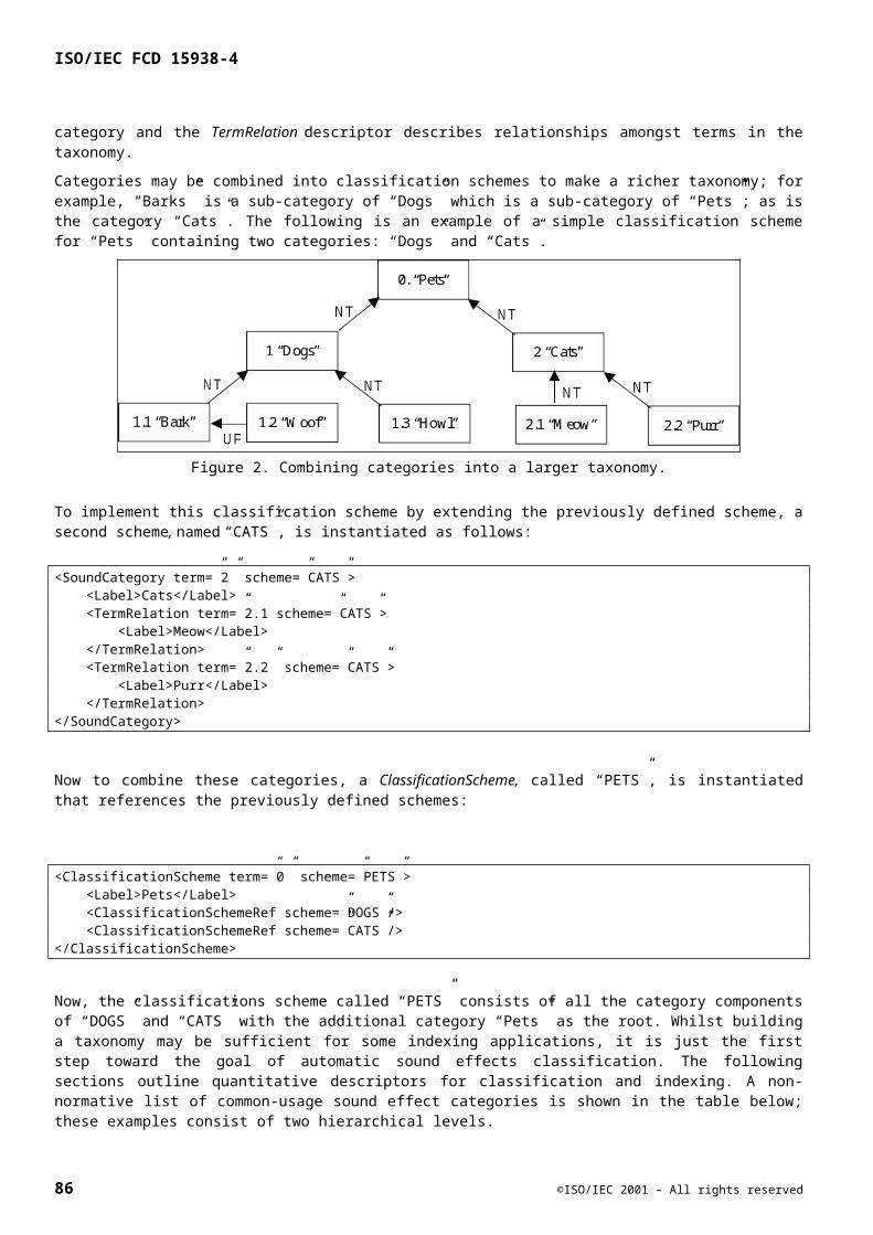
ISO/IEC FCD 15938-4

subsumes derivations of SAMPA such as XSAMPA, SAMPROSA and SAMPA-C. The SAMPROSA use of "..." as silence is encouraged.

IPASymbol. Symbol strings from the international phonetic association alphabet (IPA). This is encoded as unicode

IPANumber. Numbers from the IPA of the form "XXX", where XXX is the 3 digit IPA index. A phone made up from two or more such numbers should concatenate the numbers thus: XXXYYY...

Other. A (possibly proprietary) encoding that does not map onto any of the above

5.4.11 PhoneLexiconType

5.4.11.1 Syntax

   <complexType name="PhoneLexiconType"> <complexContent> <extension base="mpeg7:LexiconType"> <sequence> <element name="Token" type="mpeg7:PhoneType" maxOccurs="unbounded"/> </sequence> <attribute name="phoneticAlphabet" type="mpeg7:phoneticAlphabetType" use="default" value="SAMPA"/> </extension> </complexContent> </complexType>

5.4.11.2 Semantics

Name Definition

PhoneLexiconType A lexicon of phones

Token An entry in the lexicon of type PhoneType

phoneticAlphabet The name of the encoding scheme of the phone lexicon

5.4.12 SpokenContentLatticeType

5.4.12.1 Syntax

   <complexType name="SpokenContentLatticeType"> <complexContent> <extension base="mpeg7:AudioDSType">


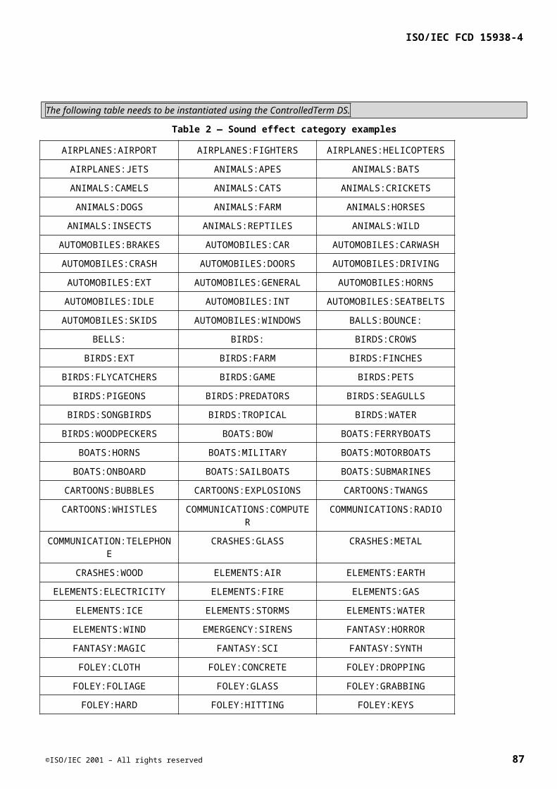
ISO/IEC FCD 15938-4

<sequence> <element name="Block" maxOccurs="65536"> <complexType> <sequence> <element name="MediaTime" type="mpeg7:MediaTimeType"/> <element name="Node" maxOccurs="65536"> <complexType> <sequence> <element name="WordLink" minOccurs="0" maxOccurs="127"> <complexType> <complexContent> <extension base="mpeg7:SpokenContentLinkType"> <attribute name="word" type="mpeg7:WordType" use="required"/> </extension> </complexContent> </complexType> </element> <element name="PhoneLink" minOccurs="0" maxOccurs="127"> <complexType> <complexContent> <extension base="mpeg7:SpokenContentLinkType"> <attribute name="phone" type="mpeg7:PhoneType" use="required"/> </extension> </complexContent> </complexType> </element> </sequence> <attribute name="num" type="mpeg7:SpokenContentNodeCountType" use="required"/> <attribute name="timeOffset" type="mpeg7:unsigned16" use="required"/> <attribute name="speakerInfo" type="uriReference" use="optional"/> </complexType> </element> </sequence> <attribute name="defaultSpeakerInfo" type="uriReference" use="required"/> <attribute name="num" type="mpeg7:SpokenContentBlockCountType" use="required"/> <attribute name="audio" use="default" value="speech"> <simpleType>   <restriction base="NMTOKEN"> <enumeration value="unknown"/> <enumeration value="speech"/> <enumeration value="noise"/> <enumeration value="noisySpeech"/> </restriction> </simpleType> </attribute> </complexType> </element> </sequence> </extension> </complexContent> </complexType>


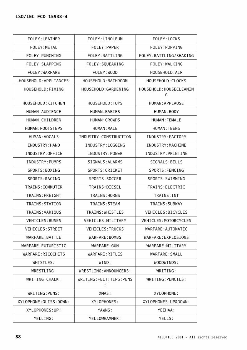
ISO/IEC FCD 15938-4

5.4.12.2 Semantics

Name Definition

SpokenContentLatticeType The main container for the ASR information. The lattice core is a series of nodes and links. Each node contains timing information and each link contains a word or phone. The nodes are partitioned into blocks to speed access.

Block A SpokenContentLatticeType consists of blocks, each block consisting of nodes. A block is defined as a lattice with an upper limit on the number of nodes that it can contain. The upper limit is to enable a compact representation for the data types which administrate the block. For instance, restricting the number of nodes in a block to 65536 enables the use of a 16 bit data type for the node number. In addition, the block represents a suitable granularity at which to represent audio quality.

MediaTime The start time and, optionally, the duration of the block. For a description of the MediaTimeType, see part 5.

Node A node within the block

WordLink A link between two nodes representing word information

word The word represented by the link

PhoneLink As a WordLink, but representing phone information

phone The phone represented by the link

num The number of this node. Node numbers range from 0 to an upper limit defined by the size of SpokenContentNodeCountType

timeOffset The time offset of this node, measured in one-hundredths of a second, from the beginning of the containing block. The absolute time is obtained by combining the block time with the node offset

speakerInfo A reference to the SpeakerInfo corresponding to this node.

defaultSpeakerInfo A reference to a SpeakerInfoType describing the default speaker. This reference is used where the speaker entry on a node in this lattice is blank. A typical use would be where there is only one speaker represented in the lattice, in which case it would be wasteful to put the same information on each node. In the extreme case that every node has a speaker reference, the defaultSpeaker is not used, but must contain a valid reference. Note that a reference outside the current description placed on every node may lead to a very large description.

num The number of this block. Block numbers range from 0 to an upper limit defined by the size of SpokenContentBlockCountType.

audio A measure of the audio quality pertinent to this block, which facilitates a crude segmentation:

unknown: No information is available.

speech: The signal is known to be clean speech, suggesting a high


ISO/IEC FCD 15938-4

Name Definition

likelihood of a good transcription.

noise: The signal is known to be non-speech. This may arise when segmentation would have been appropriate but inconvenient.

noisySpeech: The signal is known to be speech, but with facets making recognition difficult. For instance, there could be music in the background.

5.4.13 SpokenContentLinkType

5.4.13.1 Syntax

   <complexType name="SpokenContentLinkType" abstract="true"> <attribute name="probability" type="mpeg7:zeroToOneType" use="default" value="1.0"/> <attribute name="nodeOffset" type="mpeg7:SpokenContentNodeCountType" use="default" value="1"/> </complexType>

5.4.13.2 Semantics

Name Definition

SpokenContentLinkType The structure of a word or phone link in the lattice

probability The probability of this link. In a crude sense, this is to indicate which links are more likely than others, with larger numbers indicating higher likelihood. More correctly, the sum of the probabilites of each word link leaving a particular node must be less than or equal to unity. The same constraint applies to the phone links.

nodeOffset The node to which this link leads, specified as a relative offset and defaulting to 1. A node offset leading out of the current block implicitly refers to the next block. A node offset cannot span a whole block, ie., a link from a node in block 3 must lead to a node in block 3 or block 4.

5.4.14 Usage, extraction and examples (Informative)

5.4.14.1 Extraction

The Spoken Content set of DSs is designed to be a superset of the output capabilities of most ASR systems on the market at the time of publication. In this sense, the extraction method is highly non-normative; distinct from the Low Level Descriptors in this document.

Commercial large vocabulary speech recognition tends to be aimed at the dictation application area. The ideal output from a user’s point of view for this area is a “best pass” – a single hypothesis about what was spoken. This can be stored trivially as a lattice containing a single path. Some commercial recognisers also provide “word alternatives”; these can be represented as a lattice by assuming that each word alternative begins and ends at the


ISO/IEC FCD 15938-4

same time node. ASR systems used in research organisations tend to be capable of producing lattices as a basic output format.

The structure of the Spoken Content is designed to accommodate some of the errors inherent in ASR. Such errors fall into three different categories:

a) Basic decoding errors. State of the art ASR is currently limited by the underlying (usually Hidden Markov Model) technology. Even though the technology improves each year, ASR systems still make basic mistakes in recognition. It is usually difficult to determine the reason for an individual mistake, but it is generally accepted that factors such as background noise, non-canonical pronunciation, strong intonation, dialects and accents all influence recognition performance negatively. The fundamental problem, however, is that ASR systems can not yet utilise all the semantic and pragmatic knowledge that humans use to disambiguate between the many different ways in which a speech signal can be interpreted. A lattice can be used to efficiently represent multiple hypotheses about the correct transcription and their relative likelihoods.

b) Multiple hypotheses. Without sufficient contextual knowledge, the recogniser is unable to distinguish some phrases with either the same or similar phonetic content (see, e.g., Figure 1). The phrase “Recognise speech” is often cited as being misrecognised as “wreck a nice beach”. To work around this problem, state of the art ASR systems often use a word lattice representation to allow all hypothesised word sequences within the context about which they are confident. The MPEG-7 representation caters for such a lattice.

c) Unknown words. A typical state of the art ASR system has a dictionary of perhaps 20,000 to 50,000 words, and cannot produce words outside that vocabulary. Unfortunately, many discriminative (in the sense of information retrieval) words are very uncommon, and will be out of vocabulary (OOV). Typically, names of people and places fit into this category. In general, the ASR system will either omit or replace an OOV word with a phonetically similar within vocabulary word, often corrupting nearby decodings. To prevent OOV words being simply replaced by within vocabulary words, a phonetic representation is available as a lower level semantic representation (see, e.g., Figure 2).

Figure 16 — A hypothetical decoding of the phrase “Please be quite sure”. The phrases “be quite” and “beak white” have identical phonetic representations and so may only be distinguished by higher level

semantic knowledge

The underlying assumption is that ASR will not provide perfect decodings within the foreseeable future.

The Spoken Content DSs allow representation of various types of valuable information:


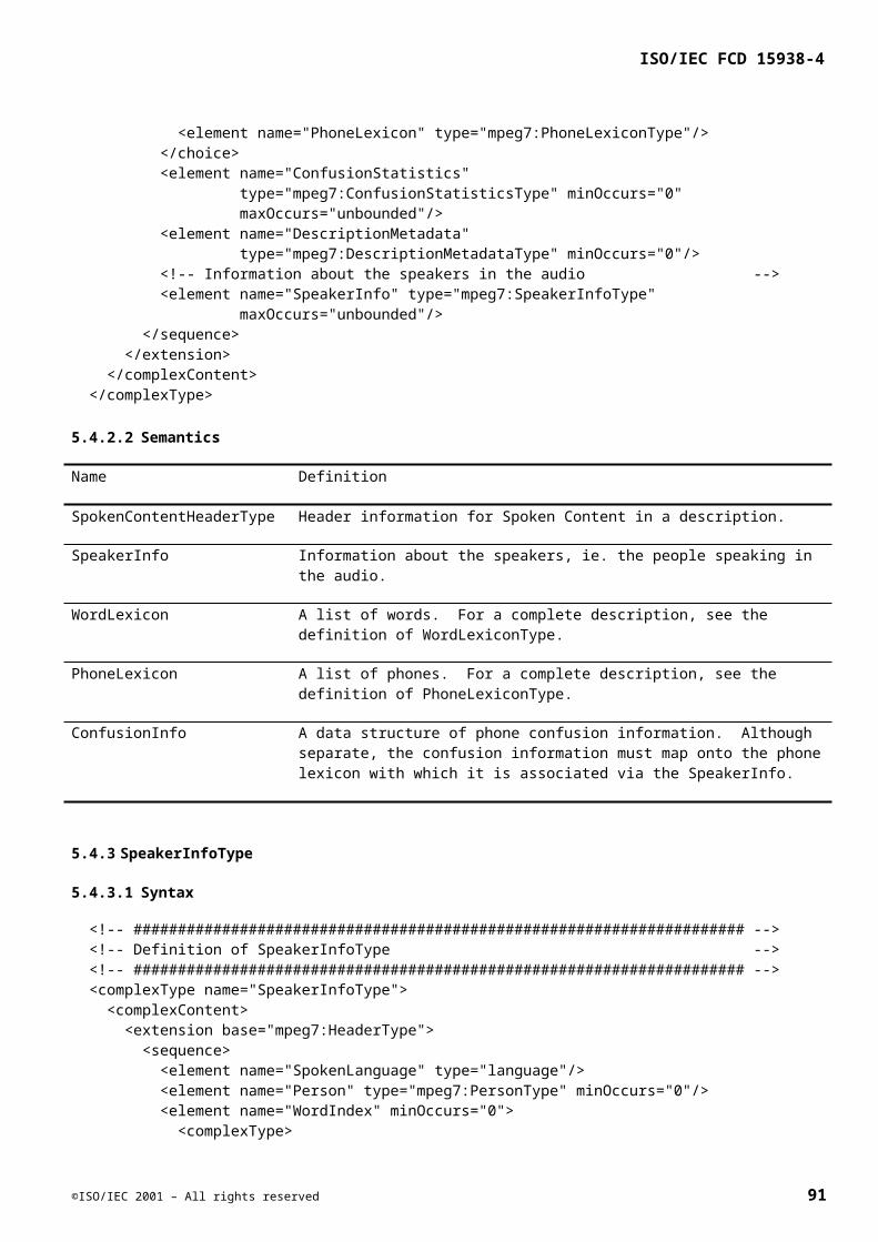
ISO/IEC FCD 15938-4

a) Linguistic: Multiple speakers are supported. In addition, the DS is capable of supporting different languages as well as people mixing languages during dialogue.

b) Semantic: The combination of words and phones allows retrieval at different semantic levels. Simple keyword searching over any annotation is unlikely to handle complexities such as anaphoric pronouns or deixis. However, it is possible to perform, e.g., anaphoric resolution on the output of an ASR to produce an annotation stream that may be more readily searched. Although storable in any scheme defined for the ASR output, it is essential that it be marked as coming from a different source. Likewise, were hand-annotated metadata available, this too can be stored in the same scheme as the ASR output. A provenance indicator is provided to distinguish between these data sources.

5.4.14.2 Structure of Spoken Content

The DS structure consists of a number of combined word and phone lattices. A lattice is an acyclic directed graph. It represents different parses of a stream of (audio) data. It is not simply a sequence of words with alternatives. One phone can be substituted for one or more phones, one word can be substituted for one or more words or phones, and that whole structure can form a substitution for one or more words or phones. The lattice structure is designed to handle certain common scenarios:

Single best path word decoding, e.g., a film annotation derived from the script.

N-Best word list, e.g., the output of some ASRs

N-Best utterance list1), the output of most ASRs

Single best path phone decoding, e.g., a phonetic representation of a word

Word lattice

A pure phone lattice, e.g., this may be produced by annotation performed on low CPU devices where full ASR is not possible.

Combined word and phone lattice to support later retrieval of OOV words.

Topic labels/predefined taxonomy/or textual summaries of the speech stream, e.g., obtained from parsing methods or textual précis.

The particular level of detail retained in the lattice is up to the annotator. For cases where most words have a high confidence but a few have low confidence (possibly indicating OOV words) we could imagine a relatively thin word lattice with occasional phone additions. For cases of decoding performed on low CPU mobile devices, a purely phone lattice may be appropriate.

Figure 2 shows a simple lattice structure for a single speaker. Each textual entry represents a word or phone, and the small circles represent nodes. Each link between nodes has associated with it a probability, or score, which represents the confidence in that particular decoding (not shown). The lattice is parsed from left to right.

1) The only difference between an N-Best utterance list and a lattice is the density of the data. The former grows exponentially with the number of hypotheses at any stage, whereas the latter is linear. For long utterances, and especially continuous annotation, the N-Best list is prohibitively large.


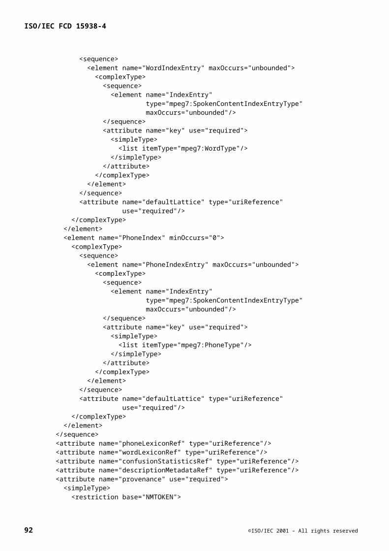
ISO/IEC FCD 15938-4

Figure 17 — A lattice structure for an hypothetical (combined phone and word) decoding of the expression “Taj Mahal drawing …”. It is assumed that the name ‘Taj Mahal’ is out of the vocabulary of the ASR system.

5.4.14.3 Example

<Header xsi:type="SpokenContentHeaderType">  <WordLexicon id="wlZero" numOriginalEntries="1000"> <Token>draw</Token> <Token>drawing</Token> <Token>hal</Token> <Token>in</Token> <Token>ma</Token> <Token>mar</Token> <Token>tar</Token> <Token>touch</Token> </WordLexicon>   <PhoneLexicon id="plZero" numOriginalEntries="10" phoneticAlphabet="other"> <Token>ae</Token> <Token>ah</Token> <Token>ax</Token> <Token>ch</Token> <Token>d</Token> <Token>hh</Token> <Token>jh</Token> <Token>l</Token> <Token>m</Token> <Token>t</Token> </PhoneLexicon> <ConfusionStatistics id="ciZero" numDimensions="10"> <InsertionCount> 10 10 10 2 50 5 5 105 10 10 </InsertionCount> <DeletionCount> 1 9 21 2 9 2 1 5 1 10 </DeletionCount> <SubstitutionCount dim="10 10"> 10 10 10 10 10 10 10 10 10 10 10 10 10 10 10 10 10 10 10 10 10 10 10 10 10 10 10 10 10 10 10 10 10 10 10 10 10 10 10 10 10 10 10 10 10 10 10 10 10 10 10 10 10 10 10 10 10 10 10 10 10 10 10 10 10 10 10 10 10 10 10 10 10 10 10 10 10 10 10 10 10 10 10 10 10 10 10 10 10 10


ISO/IEC FCD 15938-4

10 10 10 10 10 10 10 10 10 10 </SubstitutionCount> </ConfusionStatistics> <DescriptionMetadata id="infoZero"> <Instrument> <Tool> <FreeTerm>Some speech recognition engine</FreeTerm> </Tool> <Setting name="matchFactor" value="0.5"/> </Instrument> </DescriptionMetadata>  <SpeakerInfo id="sZero" phoneLexiconRef="plZero" confusionStatisticsRef="ciZero" wordLexiconRef="wlZero" descriptionMetadataRef="infoZero" provenance="ASR"> <SpokenLanguage>en-UK</SpokenLanguage> <Person> <Name> <GivenName initial="J">Jason</GivenName> <GivenName initial="P">Peter</GivenName> <FamilyName>Charlesworth</FamilyName> <Title>Dr</Title> </Name> </Person>  <WordIndex defaultLattice="lZero"> <WordIndexEntry key="drawing"> <IndexEntry node="0" block="1" lattice="lZero"/> </WordIndexEntry> </WordIndex>  <PhoneIndex defaultLattice="lZero"> <PhoneIndexEntry key="d ae ch"> <IndexEntry node="0" block="0"/> </PhoneIndexEntry> <PhoneIndexEntry key="ax jh m"> <IndexEntry node="2" block="0"/> </PhoneIndexEntry> </PhoneIndex> </SpeakerInfo> </Header> <AudioDS xsi:type="SpokenContentLatticeType" id="lZero">  <Block num="0" audio="noisySpeech" defaultSpeaker="sZero"> <MediaTime> <MediaTimePoint>2000-02-21T15:02:35</MediaTimePoint> </MediaTime> <Node num="0" timeOffset="0"> <WordLink nodeOffset="5" probability="0.5" word="touch"/> <WordLink nodeOffset="4" probability="0.5" word="tar"/> <PhoneLink nodeOffset="2" probability="0.45" phone="t"/> <PhoneLink probability="0.45" phone="d"/> </Node> <Node num="1" timeOffset="21"> <PhoneLink nodeOffset="2" probability="0.45" phone="ae"/> </Node> <Node num="2" timeOffset="25"> <PhoneLink nodeOffset="2" probability="0.45" phone="ax"/> </Node> <Node num="3" timeOffset="32"> <PhoneLink nodeOffset="2" probability="0.45" phone="ch"/>


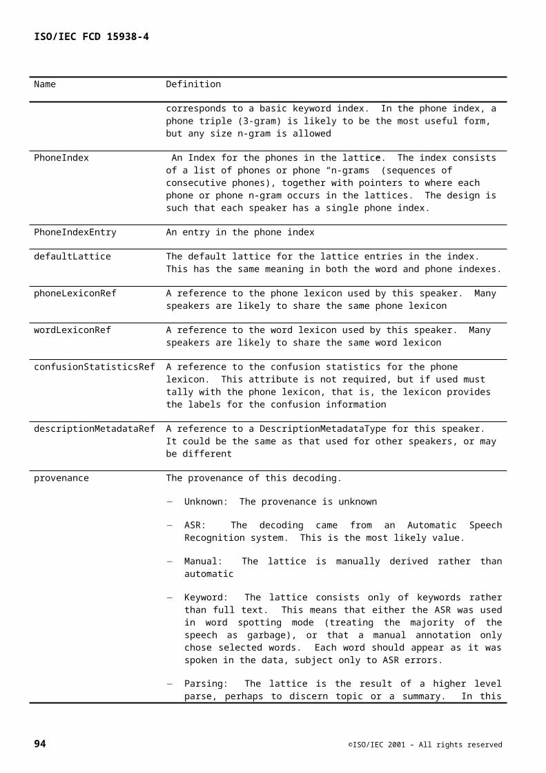
ISO/IEC FCD 15938-4

</Node> <Node num="4" timeOffset="40"> <PhoneLink probability="0.45" phone="jh"/> </Node> <Node num="5" timeOffset="50"> <WordLink nodeOffset="2" probability="0.5" word="ma"/> <WordLink nodeOffset="2" probability="0.5" word="mar"/> <PhoneLink probability="0.45" phone="m"/> </Node> <Node num="6" timeOffset="60"> <PhoneLink probability="0.45" phone="ax"/> </Node> <Node num="7" timeOffset="70"> <WordLink nodeOffset="3" probability="0.5" word="hal"/> <PhoneLink probability="0.45" phone="hh"/> <PhoneLink nodeOffset="2" probability="0.45" phone="ah"/> </Node> <Node num="8" timeOffset="80"> <PhoneLink probability="0.45" phone="ah"/> </Node> <Node num="9" timeOffset="90"> <PhoneLink probability="0.45" phone="l"/> </Node> </Block>  <Block num="1" audio="speech" defaultSpeaker="sZero"> <MediaTime> <MediaTimePoint>2000-02-21T15:02:36</MediaTimePoint> </MediaTime> <Node num="0" timeOffset="0" speaker="sZero"> <WordLink nodeOffset="2" probability="0.5" word="drawing"/> <WordLink probability="0.5" word="draw"/> </Node> <Node num="1" timeOffset="20" speaker="sZero"> <WordLink probability="0.5" word="in"/> </Node> <Node num="2" timeOffset="40" speaker="sZero"/> </Block> </AudioDS>


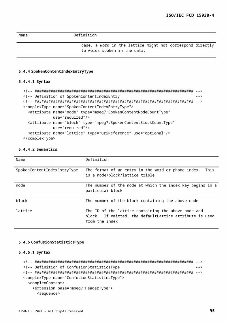
ISO/IEC FCD 15938-4

5.5 MelodyContour

5.5.1 Introduction

The MelodyContourDS is a compact representation for monophonic melodic information, which facilitates efficient and robust melodic similarity matching. The MelodyContourDS uses a 5-level contour (representing the interval difference between adjacent notes). Basic rhythmic information is also represented by storing the nearest whole-beat of each note of the melody, which can dramatically increase the accuracy of matches to a query.

5.5.2 MelodyContourType

5.5.2.1 Syntax

   <complexType name="MelodyContourType"> <complexContent> <extension base="mpeg7:AudioDSType"> <sequence> <element name="Contour" type="mpeg7:ContourType"/> <element name="Meter" type="mpeg7:MeterType" maxOccurs="unbounded"/> <element name="Beat" type="mpeg7:BeatType"/> </sequence> </extension> </complexContent> </complexType>

5.5.2.2 Semantics

Name Definition

MelodyContourType A structure containing a compact representation of the melody of the referenced segment (inherited from AudioSegment) with interval contour, meter, and beat information.

Contour The pitch contour of the melody of ContourType.

Meter The time signature(s) of the melody of MeterType.

Beat Beat information of notes in the melody of BeatType.

5.5.3 ContourType

The ContourType descriptor contains the 5-level pitch contour representation of a melody.

5.5.3.1 Syntax

    <complexType name="ContourType"> <complexContent>


ISO/IEC FCD 15938-4

<restriction base="mpeg7:AudioDType"> <sequence> <element name="ContourData" type="mpeg7:pitchContourDataType"/> </sequence> </restriction> </complexContent> </complexType>    <simpleType name="pitchContourDataType">  <list> <simpleType> <restriction base="integer"> <minInclusive value="-2"/> <maxInclusive value="+2"/> </restriction> </simpleType> </list> </simpleType>

5.5.3.2 Semantics

Name Definition

ContourType A structure containing 5-level contour information

ContourData A series of integers ranging from -2 to +2, of ContourDataType, derived from list.

The ContourData values, restricted from –2 to +2, are quantized by examining the change in the original interval value in cents. A deviation of one cent is defined as a frequency shift of 2±1/1200. One octave corresponds to 1200 cents and in equal temperament (spaced logarithmically) each semitone is 100 cents distant from the adjacent semitone below or above. The contour interval values are to be quantized according to the following table:

Table 3 — Melodic contour intervals

Contour value Change in interval

-2 Descent of at least 250 cents

-1 Descent of between 50 and 249 cents

0 No change or change of < 50 cents

1 Ascent of between 50 and 249 cents

2 Ascent of at least 250 cents

In terms of standard Western-tuning intervals, a change of a semitone or a whole-tone is represented by a value of ±1 and changes of a minor-third or greater are represented by ±2. A repeated note is represented by a value of 0.

5.5.4 MeterType

The Meter defines the time signature(s) of an audio segment, which is necessary for determining rhythmic information (strong vs. weak beats) of MelodyContourType data. A time signature is indicated by two values.


ISO/IEC FCD 15938-4

The numerator defines the number of beats per measure. The denominator defines the chosen unit of measurement of beats (whole note=1, half-note=2, quarter-note=4, etc.). Examples of common time signatures are 4/4, 2/4, and 3/4. A few examples of less common time signatures are 11/8 and 19/16.

5.5.4.1 Syntax

   <complexType name="MeterType"> <complexContent> <extension base="mpeg7:AudioDType"> <sequence> <element name="Numerator"> <simpleType>  <restriction base="integer"> <minInclusive value="1"/> <maxInclusive value="128"/> </restriction> </simpleType> </element> <element name="Denominator"> <simpleType>  <restriction base="integer"> <enumeration value="1"/> <enumeration value="2"/> <enumeration value="4"/> <enumeration value="8"/> <enumeration value="16"/> <enumeration value="32"/> <enumeration value="64"/> <enumeration value="128"/> </restriction> </simpleType> </element> </sequence> </extension> </complexContent> </complexType>

5.5.4.2 Semantics

Name Definition

MeterType The time signature(s) of the melody.

Numerator Includes integer values (from 1 to 128) for the numerator of the time signature.

Denominator Includes integer powers of two (1, 2, 4,…, 128) for the denominator of the time signature.

5.5.5 BeatType

The BeatType descriptor contains a basic rhythmic representation of a melody.


ISO/IEC FCD 15938-4

5.5.5.1 Syntax

   <complexType name="BeatType"> <complexContent> <extension base="mpeg7:AudioDType"> <sequence> <element name="BeatData"> <simpleType> <list itemType="integer"/> </simpleType> </element> </sequence> </extension> </complexContent> </complexType>

5.5.5.2 Semantics

Name Definition

BeatType A structure containing beat information. The first note of a melody is labeled with its beat number within a measure (truncated to a whole beat). Successive notes increment the beat number according to their position relative to the first note, again truncating to a whole beat. Changes in meter are indicated when the beat number reverts to a value of 1.

BeatData The beat information is stored simply as a series of integers. The data structure is of BeatDataType, derived from list. When used in conjunction with melodic ContourData, the number of elements in the list should be one more than the number of contour intervals in ContourData.

The nearest whole beat is determined by truncation. If a melody has an initial meter of n/d, the nearest whole beat must be an integer ranging from 1 to n. For example, if a melody starts on beat 2.5, 2.75, or 2.99999, the BeatData would begin with a value of 2 (as long as n?≥?2). The next BeatData value would be the difference in whole beat numbers from the first value.

5.5.6 Usage and examples (Informative)

There are many examples of applications for the MelodyContour description scheme. The most obvious is the “query-by-humming” problem, in which a song is automatically identified from an audio input (such as a person humming). When identifying a melody, the listener perceives not only the pitches of the melody, but how those pitches correspond to particular moments in time (i.e. rhythm). The following simple example illustrates the importance of rhythm in melodic description.

Figure 18 — First four notes of the Bridal Chorus from Lohengrin (Wagner), a.k.a. Here Comes the Bride.


ISO/IEC FCD 15938-4

Figure 19 — First four notes of O Tannenbaum.

It is apparent that these are two very distinct melodies, yet the sounding pitches are identical. The difference lies not only in the respective meters (time signatures) of the songs, but in the position of the notes relative to the metric structure of each piece. The time signature of the first example is 4/4, and the strong beats occur on the first and third beats of a measure, which correspond to the first and third notes of the piece. The second example has a time signature of 3/4, and the strong beat is on the first beat of the measure, corresponding to the second note. The MelodyContourDS was designed to unambiguously resolve these two melodies.

  <AudioDS xsi:type="MelodyContourType"> <Contour> <ContourData>2 0 0</ContourData> </Contour>  <Meter> <Numerator>4</Numerator> <Denominator>4</Denominator> </Meter>  <Beat> <BeatData>1 2 2 3</BeatData> </Beat> </AudioDS>

  <AudioDS xsi:type="MelodyContourType"> <Contour> <ContourData>2 0 0</ContourData> </Contour>  <Meter> <Numerator>3</Numerator> <Denominator>4</Denominator> </Meter>   <Beat> <BeatData>3 4 4 5</BeatData> </Beat> </AudioDS>

The following example is an excerpt from the song “Moon River” by Henry Mancini:


ISO/IEC FCD 15938-4

Figure 3 — “Moon River”

  <AudioDS xsi:type="MelodyContourType"> <Contour> <ContourData>2 -1 -1 -1 -1 -1 1</ContourData> </Contour>  <Meter> <Numerator>3</Numerator> <Denominator>4</Denominator> </Meter>  <Beat> <BeatData>1 4 5 7 8 9 9 10</BeatData> </Beat> </AudioDS>


ISO/IEC FCD 15938-4

5.6 Melody

5.6.1 Introduction

Although useful in a wide number of situations, the MelodyContour DS in the preceding section does not capture all possible applications for a melody representation. One may wish to restore the precise notes of a melody for the purpose of auditory display. One may already know certain aspects of the piece such as key, and want to search on that criterion. The five-level quantisation undergone for the MelodyContour is inherently lossy, and may cause ambiguities among similar melodies. The Melody DS fills the above expanded needs as a representation that retains maximal information about a melody—allowing for reconstruction of the melody, as well as keeping other features—while still allowing for compact, efficient queries. The crux of this Description Scheme is a transform into “interval space,” or encoding the successive differences between the notes of a melodic fragment into a feature vector of high precision. The feature vector is made up of the transitions between notes, i.e. pitch intervals and differences in duration. Arrayed about this core description are various support functions that describe other aspects of melody that may be of potential interest. They may be considered additional, optional tags that offer alternative means of constraining a MelodySequence search.

5.6.2 MelodyType

5.6.2.1 Syntax

   <complexType name="MelodyType"> <complexContent> <extension base="mpeg7:AudioDSType"> <sequence> <element name="MelodyMeter" type="mpeg7:MeterType" minOccurs="0"/> <element name="MelodyScale" type="mpeg7:MelodyScaleType" minOccurs="0"/> <element name="MelodyKey" type="mpeg7:MelodyKeyType" minOccurs="0"/> <element name="MelodySequence" type="mpeg7:MelodySequenceType" minOccurs="0" maxOccurs="unbounded"/> </sequence> </extension> </complexContent> </complexType>

5.6.2.2 Semantics

Name Definition

MelodySequence The body of the MelodyDS


MelodyMeter See the MelodyContour definition of MeterType

MelodyScale An array of intervals representing the (chromatic) scale steps to the point at which the scale repeats

MelodyKey A container type containing degree, alteration, and mode, with an optional keySignificance attribute. This reflects the section to which the melodic fragment is taken. The keySignificance attribute denotes how intrinsic the sense of key is to the piece (e.g. Bach's "B minor Mass").

ISO/IEC FCD 15938-4

5.6.3 MelodyMeter

The MelodyMeter descriptor uses the same datatype as the Meter descriptor in the MelodyContour DS. Please refer to that section for details.

5.6.4 MelodyScale

The MelodyScale descriptor contains a list of intervals that are typical of the tuning system used. The scale is not directly used in operations on the melody, so it is an optional descriptor, but MelodyScale may be helpful for reference purposes.

5.6.4.1 Syntax

     <complexType name="MelodyScaleType"> <simpleContent> <restriction base="mpeg7:floatVector"/> </simpleContent> </complexType>

5.6.4.2 Semantics

Name Definition

MelodyScale Array of a repeatable span of notes, in semitones from the base pitch (which is assumed, and elided). The default value is taken to be [1.0 2.0 3.0 4.0 5.0 6.0 7.0 8.0 9.0 10.0 11.0 12.0], or the equal-tempered chromatic scale. If semitones are not applicable, one may use a computational equivalent in the formula:

where F0[0] is the base pitch of the scale.

An example of a non-traditional scale is the Pierce scale, which contains 13 equally spaced notes that repeats after an octave and a fifth (a perfect twelfth, or a frequency ratio of 1:3). This scale would then be:

[1.4615 2.9231 4.346 5.8462 … 17.538 19.000]

A more appropriate scale is sought as an example.

5.6.5 MelodyKey

The MelodyKey descriptor contains the base note, with any accidental, and mode of the key. As with MelodyScale, it is not directly used in operations on the MelodySequence, and additionally is restricted to traditional western music where such a feature makes sense. MelodyKey may be modified with a flag in whether this information is integral to identification of the piece (e.g. a B minor Mass may be found in a database by using this feature in conjunction with, or in place of, a MelodySequence).


ISO/IEC FCD 15938-4

5.6.5.1 Syntax

    <complexType name="MelodyKeyType"> <complexContent> <extension base="mpeg7:AudioDSType"> <sequence> <element name="KeyNote"> <complexType> <simpleContent> <extension base="mpeg7:degreeNoteType"> <attribute name="display" type="string"/> </extension> </simpleContent> </complexType> </element> </sequence> <attribute name="accidental" type="mpeg7:degreeAccidentalType" use="default" value="natural"/> <attribute name="mode" use="default" value="major"> <simpleType> <restriction base="string"> <enumeration value="major"/> <enumeration value="minor"/> <enumeration value="otherMode"/> </restriction> </simpleType> </attribute> <attribute name="keySignificance" type="boolean" use="optional"/> </extension> </complexContent> </complexType> <simpleType name="degreeNoteType"> <restriction base="string"> <enumeration value="C"/> <enumeration value="D"/> <enumeration value="E"/> <enumeration value="F"/> <enumeration value="G"/> <enumeration value="A"/> <enumeration value="B"/> </restriction> </simpleType> <simpleType name="degreeAccidentalType"> <restriction base="string"> <enumeration value="flat"/> <enumeration value="natural"/> <enumeration value="sharp"/> <enumeration value="doubleSharp"/> <enumeration value="doubleFlat"/> </restriction> </simpleType>

5.6.5.2 Semantics

Name Definition


ISO/IEC FCD 15938-4

KeyNote The basic pitch chroma, from the Anglo-American tradition of using the alphabet from A to G. This is less an assertion of one tradition than one system being chosen as an internal representation for its brief, well-understood labels. Note again that if a Western note label is not appropriate to the application or the content, then it may be omitted.

Display An optional string to be used as an alternate display for the KeyNote. For example, "sol" for the internal "G" representation, assuming an fixed "do" system.

accidental An alteration to the basic alphabetic pitch chroma. It may be natural (default), flat, sharp, double-flat, double-sharp.

mode The mode (major, minor, or "other mode") of the piece.

5.6.6 MelodySequence

The MelodySequence is the core of the Melody DS, in its typical use. At its core, it lists an array of intervals from the first note to the subsequent note. The units used are based on logarithmic frequency, but are conveniently estimators to semi-tones. These units are applicable to nearly any musical system, however. In addition to the notes, optional lyrics, phonemes, starting notes, and alternative analyses may be included.

5.6.6.1 Syntax

   <complexType name="MelodySequenceType"> <complexContent> <extension base="mpeg7:AudioDSType"> <sequence> <element name="StartingNote" minOccurs="0"> <complexType> <sequence> <element name="StartingFrequency" type="float" minOccurs="0"/> <element name="StartingPitch" minOccurs="0"> <complexType> <sequence> <element name="PitchNote"> <complexType> <simpleContent> <extension base="mpeg7:degreeNoteType"> <attribute name="display" type="string"/> </extension> </simpleContent> </complexType> </element> </sequence> <attribute name="accidental" type="mpeg7:degreeAccidentalType" use="default" value="natural"/> <attribute name="height" type="integer"/> </complexType> </element>   </sequence> </complexType> </element>


ISO/IEC FCD 15938-4

<element name="NoteArray"> <complexType name="NoteArrayType"> <complexContent> <extension base="mpeg7:AudioDSType"> <sequence> <element name="Note" maxOccurs="unbounded"> <complexType> <sequence> <element name="Interval" type="float"/> <element name="NoteRelDuration" type="float"/> <element name="Lyric" type="mpeg7:WordType" minOccurs="0"/> <element name="PhoneNGram" minOccurs="0"> <simpleType> <list itemType="mpeg7:PhoneType"/> </simpleType> </element>  </sequence> </complexType> </element> </sequence> </extension> </complexContent> </complexType> </element> </sequence> </extension> </complexContent> </complexType>

5.6.6.2 Semantics

Name Definition

StartingNote A container for the absolute pitch in the first note in a sequence, in case of desire for reconstruction, or if absolute pitch is needed for comparison purposes.

StartingFrequency The fundamental frequency of the first note in the represented sequence in units of Hz.

StartingPitch A pitch marker using chroma (note plus accidental, as above) and pitch height

height The number of the octave of the StartingPitch, counting octaves upwards from a standard piano's lowest A as 0.

NoteArray The array of intervals, durations, and optional lyrics. In the case of multiple NoteArrays, all of the NoteArrays following the first one listed are to be interpreted as secondary, alternate choices to the primary hypothesis. Use of the alternatives is application-specific, and they are included here in simple recognition that neither segmentation nor pitch tracking are infallible in every case.

Interval The number of semitones between the previous note and the current note. Alternately, when semitones are not applicable (as in non-western scales), or when using a fundamental frequency-based estimator, one may use the following algorithm:


ISO/IEC FCD 15938-4

Note that for m notes in a sequence, there are m–1 intervals

This is a logarithmic "interval space" which has direct applicability to the western musical tradition, but which also applies to any tuning system. It lies in contrast to the MelodyContour DS in that rather than quantising the intervals, it retains all of the potential errors (in frequency estimates and humming by imperfect musicians), and lets the data set itself act as the ideal quantiser. An L2 norm between a query interval vector and the other melody vectors in the interval space is an appropriate distance metric (informative).

NoteRelDuration The log ratio of the differential onsets for the notes in the series. This is a logarithmic "rhythm space" that is resilient to gradual changes in tempo.

An extraction algorithm for extracting this is:

for , and

Where Onset[n] is the time of onset of note n in seconds (measured from the onset of the first note).

The first note duration is in relation to a quarter note at 120 beats per minute (0.5 seconds), which gives an absolute reference point for the first note.

Lyric A word or syllable associated with the note (first of the notes represented by the interval). This need not be perfectly aligned.

Phoneme An n-gram (i.e. list) of phonemes associated (i.e. sung) with the note (first of the notes represented by the interval). Syllabic breaks are not normatively specified, but are understood to follow the traditions of their language.

5.6.7 Usage, extraction, and examples (informative)

The section on MelodyContour motivated the query-by-humming applications, and covers a wide range of them with a very compact representation. However, there is the need for a melody descriptor that can cover a wider range of melody representation, for example being able to reconstruct a melodic line and lyrics from its MPEG-7 description. There are additional descriptive tags such as key that may aid in musical search. The Melody DS is a more verbose construct than the MelodyContour DS that encompasses these enhanced functionalities.

The basic theory behind the core melodic interval NoteArray is that any quantisation scheme such as that used with the MelodyContour descriptor will be imperfect in some cases. The NoteArray goes in the opposite direction and keeps all of the errors in an imperfect rendition of a melody (i.e. a query), and uses the space of target melodies as a natural vector quantisation scheme. That is, the errors fall out when the actual match takes place.

A typical matching metric among NoteArrays, for both Intervals and Durations, is an L2 norm. This would work best when matching arrays of identical lengths, but can accommodate differing dimensions by truncating or zero-padding non-conforming arrays.


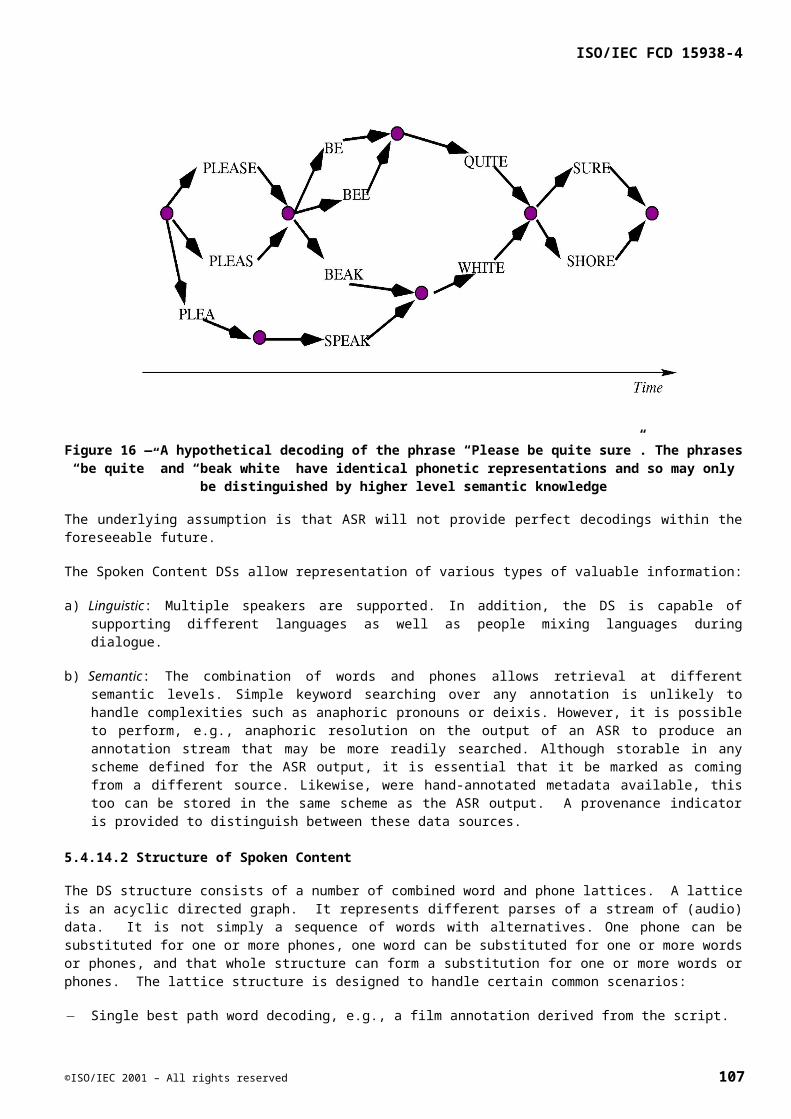
ISO/IEC FCD 15938-4

The semantics of the intervals used here are slightly biased towards an equal-tempered scale, but older tunings may use arbitrary precision, according to needs; if desired, the integral chromatic scale steps may safely be used as estimators to just-tempered scale steps as appropriate to the application.

An example instantiation for "Moon River," as shown in the MelodyContour section, is shown below:

First, the melody array is [+7 –2 –1 –2 –2 –2 +2],

And the relative duration array is [2.3219 –1.5850 1 –0.4150 –1.5650 0 0 (2)].

<AudioDS xsi:type="MelodyType"> <MelodyMeter> <Numerator>4</Numerator> <Denominator>4</Denominator> </MelodyMeter> <MelodyScale>1 2 3 4 5 6 7 8 9 10 11 12</MelodyScale> <MelodyKey mode="otherMode"> <KeyNote display="sol">G</KeyNote> </MelodyKey> <MelodySequence> <StartingNote> <StartingFrequency>391.995</StartingFrequency> <StartingPitch height="4"> <PitchNote display="sol">G</PitchNote> </StartingPitch> </StartingNote> <NoteArray>   <Note> <Interval>7</Interval> <NoteRelDuration>2.3219</NoteRelDuration> <Lyric>Moon</Lyric> <PhoneNGram>m u: n</PhoneNGram> </Note> <Note> <Interval>-2</Interval> <NoteRelDuration>-1.5850</NoteRelDuration> <Lyric>Ri-</Lyric> </Note> <Note> <Interval>-1</Interval> <NoteRelDuration>1</NoteRelDuration> <Lyric>ver</Lyric> </Note>  </NoteArray> </MelodySequence> </AudioDS>

Documents

ISO/IEC JTC 1/SC 29 N - 情報処理学会 · Web view... .doc STD Version 1.0. Élément introductif ... describing a word that is not in the vocabulary of ... find the greatest