Embed Size (px)
Citation preview
Job Search Behavior over the Business Cycle∗
Toshihiko Mukoyama
Federal Reserve Board
and
University of Virginia
Christina Patterson
Federal Reserve Bank of New York
Aysegul Sahin
Federal Reserve Bank of New York
May 2013Preliminary and incomplete
Abstract
In this paper, we study nonemployed workers’ job search behavior. In particular,
we analyze how search behavior changes over the business cycle. Theoretically, we show
that job search intensity can either be procyclical or countercyclical depending on various
factors. Empirically, we first examine how aggregate job search intensity changes over
the business cycle. Second, we examine job search behavior at the individual level and
analyze how various factors affect individuals’ job search behavior.
Keywords: job search, time use, business cycles
JEL Classifications: E24, E32, J22, J64
∗We thank Mark Aguiar, Andreas Mueller, and seminar participants at the Board of Governors, Census Bu-
reau, Concordia University, Minneapolis Fed, New York Fed, University of Calgary, and Vanderbilt University
for their comments and suggestions. We also thank Jesse Rothstein for providing us with the unemployment
insurance data, and Andriy Blokhin and Xiaohui Huang for excellent research assistance. The views expressed
in this paper are solely the responsibility of the authors’ and should not be interpreted as reflecting views of
the Board of Governors of the Federal Reserve System, the Federal Reserve Bank of New York, or any other
person associated with the Federal Reserve System.
1

1 Introduction
Search effort of firms and workers is one of the most important determinants of aggregate
employment. In a frictional labor market, a higher number of matches are formed when both
firms and workers make more effort to find a suitable counterpart. Understanding the factors
that influence search effort on both the firm and the worker sides, therefore, is essential in
analyzing the behavior of aggregate employment.
Firms’ recruiting effort decision over the business cycle has been studied extensively in the
past. For example, studies of Beveridge curves find that firms make higher recruiting effort by
posting more vacancies during booms.1 A recent paper by Davis, Faberman, and Haltiwanger
(2010) argues that firms’ recruiting effort in addition to posting vacancies also contributes to
the cyclical pattern of how firms match with workers. Relatedly, Davis, Faberman, and Halti-
wanger criticize the standard Diamond-Mortensen-Pissarides (DMP) framework for limiting
the firm’s recruiting effort just to the number of vacancies—they emphasize the importance
of other inputs in accounting for the microeconomic patterns of hiring.
In this paper, we focus on the worker side of the labor market to analyze how workers’
job search effort varies over the business cycle. We show that just counting the number
of nonemployed workers (or unemployed workers) is not sufficient to measure workers’ job
search effort. In that sense, our paper complements Davis, Faberman and Haltiwager’s (2010)
argument and extends their critique to the measurement of search effort on the worker side.
Workers’ search effort has not been studied much in the macroeconomic literature both
theoretically and empirically. In the basic DMP model (as in Pissarides (1985) and Shimer
(2005)), a firm makes an explicit recruiting effort choice by deciding how many vacancies to
post, while a nonemployed worker waits passively until a job offer arrives. In other words, the
basic DMP search and matching models abstract from workers’ intentional choice of search
effort and workers’ search decisions play no role in facilitating match formation.
There are a few recent theoretical papers that analyzes the worker’s search effort explicitly.
1See, for example, Blanchard and Diamond (1990) and Shimer (2005).
2

In the model of Christiano, Trabandt, and Walentin (2012), search effort by nonemployed
households moves procyclically, and this generates procyclical employment. In Veracierto
(2008) and Shimer (2011), a nonemployed worker can choose whether being “unemployed”
or “inactive,” and only unemployed workers have a positive probability of finding a job (while
they have to incur a cost of search). This discrete choice between “unemployed” or “inactive”
can be considered as a discrete choice of search effort.
In some of these models, such as Veracierto (2008) and Christiano, Trabandt, and Walentin
(2012), the fluctuations of employment and unemployment are driven solely by the worker’s
search effort. In other words, in these models, the employment fluctuations are entirely
supply driven, while in the basic DMP model, employment fluctuations are entirely demand
driven. These are completely opposite views on the aggregate labor market fluctuations, and
the procyclical search effort by workers is an essential part of the cyclical dynamics in the
former class of models. Thus, examining the cyclical behavior of workers’ search effort can
provide valuable information on the source of the fluctuations in the labor market.
Despite its importance, there is even less work done on the empirical analysis of the
worker’s search effort that goes beyond the measurement of unemployment.2 The main
reason for this oversight is the lack of high quality data on job search behavior. We overcome
this obstacle by combining two datasets as we describe later.
Beyond the determination of aggregate employment, workers’ search effort also has im-
portant implications for policy design. For example, in the recent studies of optimal un-
employment insurance over the business cycle, such as Kroft and Notowidigdo (2011) and
Landais, Michaillat, and Saez (2011), moral hazard in worker’s search effort (and how it
varies over the business cycle) is the central focus in determining the optimal policy.
The paper consists of three parts. We first construct a simple model in order to obtain
theoretical predictions on how economic environment influences the worker’s job search effort.
One insight we learn from the model is that there is no ex ante reason to believe that the
2There are a few important exceptions, which we discuss below.
3

job search effort is procyclical or countercyclical. There are many effects at work, and it is
an empirical question whether some effects dominate others.
Second, we document the macroeconomic time series properties of job search effort. We
use the American Time Use Survey (ATUS) and the Current Population Survey (CPS) in
order to measure job search effort at the aggregate and individual level. Both datasets have
their own shortcomings, and our innovation is to combine the information from both surveys
in order to obtain a nationally-representative and monthly time series of job search effort.
In an analogy to the labor supply literature, we distinguish two different margins of search
effort: the “extensive margin” and the “intensive margin.” The “extensive margin” refers to
“how many nonemployed workers engage in search activities, ” while the “intensive margin”
refers to “how intensely each searcher is searching.” Aggregate search effort in the economy
then can be calculated as the product of the extensive and intensive margins.
Third, we explore the determinants of the job search effort, by looking at the individual
level. In particular,we run regressions of individual search effort on worker characteristics and
measures of their economic environment. We are particularly interested in the relationship
of search effort with with labor-market tightness and wealth level.
There are existing papers that utilize the ATUS and the CPS to measure the search effort.
Shimer (2004) is an early critic of the way search effort is modeled in typical search-matching
models. Shimer uses the CPS measure of job search intensity and shows that the procyclical-
ity of search effort, which is the implication of existing models of job search, is not supported
by the data. Krueger and Mueller (2010) and Aguiar, Hurst, and Karabarbounis (2012) are
two more recent papers which make use of the ATUS to analyze job search behavior. De-
Loach and Kurt (2012) look at ATUS and analyze the determinants of the search time at the
micro level. Compared to these studies, our analysis has the advantage of a better measure
of job search effort that utilizes information from both the ATUS and the CPS.
This paper is organized as follows. Section 2 presents a simple model in order to uncover
the elements that affect the cyclicality of search behavior at the macro and micro level.
4

Section 3 describes the data and explains how we combine the information from two datasets.
Section 4 analyzes the cyclicality of search effort at the macro level. Section 5 investigates
why we observe the countercyclical search effort from the micro level. Section 6 concludes.
2 Model
In this section, we formulate a simple static model of individual search decision. The model
serves two purposes. First, it shows that whether nonemployed workers’ search effort is
procyclical or countercyclical is an empirical question—within reasonable settings of the
model, search effort can be procyclical or countercyclical. The models of Appendix A confirm
this finding in a more elaborate, dynamic setting. Second, it clarifies the intuition regarding
the channels that contribute to the cyclicality of search effort. In particular, the model
focuses on the effect of labor-market tightness (how many vacancies there are compared to
the number of unemployed workers), wages, unemployment compensations, and wealth.
2.1 Setting
Consider a worker who is currently nonemployed. In the beginning of the period, she decides
the intensity of job search effort, s ∈ R+. Search effort is costly, and we assume that the cost
(in utility term) is c(s) where c′(·) > 0 and c′′(·) > 0. The job-finding probability is assumed
to take the form f(s, s, θ) where f is increasing and concave in s. The variable s is the search
effort of other workers. s affects the job-finding probability of a given worker when there is
an externality: for example, it may be the case that when some workers search harder, it
reduces the odds of other workers finding a job. θ is a parameter that represents the labor
market condition surrounding the worker. Later, θ is represented by vacancy-unemployment
ratio. We assume that f is increasing in θ.
A special case is the standard DMP model, which postulates a constant-returns-to-scale
matching function M(u, v). There, the number of matches, M(u, v), is increasing in both the
number of unemployed workers u and the number of vacancies posted v. Given the constant
5
returns, the probability of a worker matching with a job is M(u, v)/u = M(1, θ), where θ
is defined as the vacancy-unemployment ratio v/u. This formulation is a special case in the
sense that f(s, s, θ) = M(1, θ) and it does not depend on s and s.
A less trivial special case is the one analyzed by Pissarides (2000, Chapter 5) where job
search effort is explicitly modeled. The matching function at the aggregate level (assuming
that the individuals are atomistic) is assumed to take the form M(su, v) where M(su, v)
is constant-returns-to-scale (and increasing) in these two terms. For each individual, the
probability of finding a job is sM(su, v)/(su) which can be rewritten as3
f(s, s, θ) = sM
(1,
1
sθ
). (1)
where θ is defined as v/u.
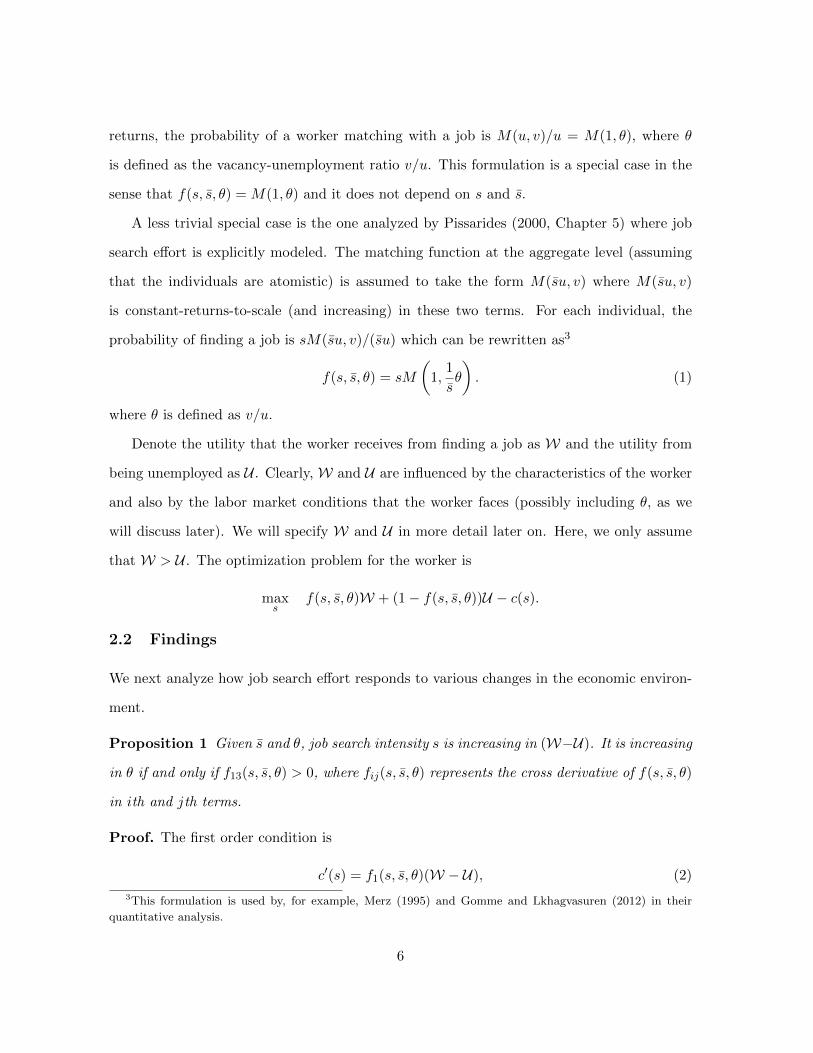
Denote the utility that the worker receives from finding a job as W and the utility from
being unemployed as U . Clearly, W and U are influenced by the characteristics of the worker
and also by the labor market conditions that the worker faces (possibly including θ, as we
will discuss later). We will specify W and U in more detail later on. Here, we only assume
that W > U . The optimization problem for the worker is
maxs
f(s, s, θ)W + (1− f(s, s, θ))U − c(s).
2.2 Findings
We next analyze how job search effort responds to various changes in the economic environ-
ment.
Proposition 1 Given s and θ, job search intensity s is increasing in (W−U). It is increasing
in θ if and only if f13(s, s, θ) > 0, where fij(s, s, θ) represents the cross derivative of f(s, s, θ)
in ith and jth terms.
Proof. The first order condition is
c′(s) = f1(s, s, θ)(W −U), (2)
3This formulation is used by, for example, Merz (1995) and Gomme and Lkhagvasuren (2012) in their
quantitative analysis.
6

where fi(s, s, θ) is the partial derivative of f(s, s, θ) with respect to ith term. From the
Implicit Function Theorem,
ds
d(W −U)=
f1(s, s, θ)
c′′(s)− f11(s, s, θ)(W −U)
Since c′′(s) > 0, f11(s, s, θ) ≤ 0, and f1(s, s, θ) ≥ 0, ds/d(W −U) ≥ 0. Similarly,
ds
dθ=
f13(s, s, θ)(W −U)
c′′(s)− f11(s, s, θ)(W −U)
and since c′′(s) > 0 and f11(s, s, θ) ≤ 0, andW−U > 0, ds/dθ has the same sign as f13(s, s, θ).
In words, f13(s, s, θ) > 0 means that the individual’s search effort s and the labor mar-
ket condition θ are complementary—when θ increases, the “marginal product” of s increases.
This is the situation where it is productive to search harder when the firms are posting many
vacancies. The opposite case, f13(s, s, θ) < 0, can be considered as the case where s and
θ are substitutive in the job matching process. This happens, for example, in a situation
where matches are formed no matter what individual workers do because firms are sending
out many offers to everyone.
Note that in the standard DMP model, (W − U) also has a direct link to θ in general
equilibrium, which we ignore here.4 Appendix A shows that even in a fully dynamic and
general equilibrium model, an equation similar to (2) determines s and the main message of
this section (the cyclicality of s depends on the setting of the model) carries through.
Proposition 1 provides an analysis of individual search effort decisions. When we look at
the data, we need to take into account that s is also determined (by the choice of s of other
4There, both θ and (W − U) are endogenous, and it is difficult to think of an experiment of “moving θ
exogenously” as we do here. In that case, if, for example, the outcome of the match is expected to be good,
the high surplus from the match is divided between firms and workers through Nash bargaining (therefore a
high (W −U)), while a high surplus for firms leads to more vacancy posting today (therefore a high θ). This
effect increases both (W −U) and θ at the same time. Perhaps a more straightforward “partial equilibrium”
intuition is that θ at time t would affect the unemployment at time t+ 1, and this affects (W−U) in the next
period. This intuition is correct only in a partial-equilibrium model. In the general equilibrium of Pissarides
(1985) model, (W−U) is not affected by u at time t+1 and thus there is no effect going through this channel.
7

people) in the economy and influenced by the economic environment. For simplicity, suppose
that the economy consists of homogeneous workers. Then, in a symmetric equilibrium,
s = s has to hold. Under this assumption, we can show prove the “equilibrium version” of
Proposition 1. First, we need an additional assumption.
Assumption 1 c′′(s)− (f11(s, s, θ) + f12(s, s, θ))(W −U) > 0 for all s and θ.
This is satisfied when f12(s, s, θ) is sufficiently small. It is, for example, satisfied under (1)
since there f12(s, s, θ) is negative. Under Assumption 1, it is straightforward to show the
following.
Proposition 2 Given θ, job search intensity, s, is increasing in (W − U). It is increasing
in θ if and only if f13(s, s, θ) > 0.
The proof is omitted since it is similar to the proof of Proposition 1. Thus the result of this
“equilibrium outcome” is similar to the outcome of the decision problem in Proposition 1.
Note that this result is still not “general equilibrium” in the sense of Pissarides (2000), since
variables such as θ, W, and U are assumed to be exogenous. We take the current approach
because we are interested in the workers’ search effort decision in a given environment.
To characterize the determinants of W and U , we make the following additional assump-
tions. First, the utility from consumption is represented by a strictly increasing and strictly
concave utility function u(c), where c is consumption. The worker has an asset level a. If
he works, he receives the wage w, and if he is unemployed, he receives the unemployment
compensation b. Thus, c = w + a if he works and c = b + a if he is unemployed. Then,
W = u(w + a) and U = u(b + a). (In a dynamic model, c also depends on the expectations
on future income.) Assume that w > b. Then it is straightforward to show the following.
Corollary 1 The job search intensity, s, is increasing in w, decreasing in b, and decreasing
in a in the context of both Propositions 1 and 2.
Proof. We only need to establish how W − U responds to these parameters since we can
then apply Propositions 1 and 2, we Since W − U = u(w + a) − u(b + a), the first two are
8

straightforward. For a,
d(W −U)
da= u′(w + a)− u′(b+ a) < 0
since w + a > b+ a.
During expansions, θ, w, and a are typically higher. The first can have positive or negative
effect in s, depending on the f(s, s, θ) function. The second has a positive effect and the
third has a negative effect.5 Therefore, whether s is procyclical or countercyclical for a
nonemployed worker is an empirical issue. This in particular raises two distinct empirical
questions: (i) the relative strengths of the effect of w and a, and (ii) the shape of the f(s, s, θ)
function. At the macroeconomic level, the number of nonemployed worker also fluctuates,
adding one more factor in the fluctuations of the aggregate search effort.
2.3 Generalizing the matching function
Before discussing our empirical analysis, one issue is worth exploring: when is f13(s, s, θ)
negative? This is not a trivial question—for example, when we start from the aggregate
matching function, a natural formulation such as (1) cannot generate a negative f13(s, s, θ):
f13(s, s, θ) is always positive as long as M(su, v) is increasing in v. As we discussed earlier,
intuitively, it is quite natural to think of a situation where f13(s, s, θ) is negative—that is, the
“marginal product” of individuals’ search is smaller when the labor market conditions are
better. For example, when there are so many jobs (the firm searches very heavily), that it is
almost certain that every worker has a good job offer, additional effort by the worker does
not add much to the matching outcome. Based on a similar intuition, Shimer (2004) builds a
concrete micro-founded matching model which does not necessarily result in complementarity
between worker search effort and the labor market conditions.
As an example of “generalized” version of (1), we can consider
f(s, s, θ) = χ
(αsψ + (1− α)
(ss
)ξθψ)η
. (3)
5If the utility function is linear, the third effect is absent.
9
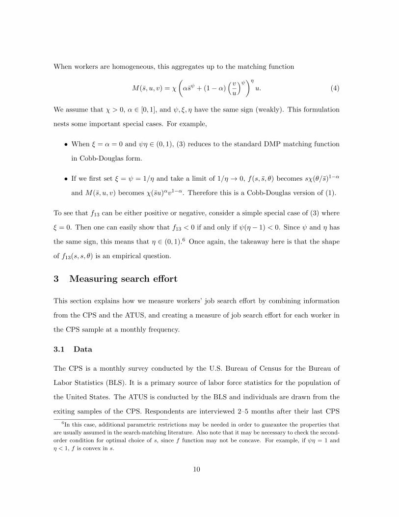
When workers are homogeneous, this aggregates up to the matching function
M(s, u, v) = χ
(αsψ + (1− α)
(vu
)ψ)ηu. (4)
We assume that χ > 0, α ∈ [0, 1], and ψ, ξ, η have the same sign (weakly). This formulation
nests some important special cases. For example,
• When ξ = α = 0 and ψη ∈ (0, 1), (3) reduces to the standard DMP matching function
in Cobb-Douglas form.
• If we first set ξ = ψ = 1/η and take a limit of 1/η → 0, f(s, s, θ) becomes sχ(θ/s)1−α
and M(s, u, v) becomes χ(su)αv1−α. Therefore this is a Cobb-Douglas version of (1).
To see that f13 can be either positive or negative, consider a simple special case of (3) where
ξ = 0. Then one can easily show that f13 < 0 if and only if ψ(η − 1) < 0. Since ψ and η has
the same sign, this means that η ∈ (0, 1).6 Once again, the takeaway here is that the shape
of f13(s, s, θ) is an empirical question.
3 Measuring search effort
This section explains how we measure workers’ job search effort by combining information
from the CPS and the ATUS, and creating a measure of job search effort for each worker in
the CPS sample at a monthly frequency.
3.1 Data
The CPS is a monthly survey conducted by the U.S. Bureau of Census for the Bureau of
Labor Statistics (BLS). It is a primary source of labor force statistics for the population of
the United States. The ATUS is conducted by the BLS and individuals are drawn from the
exiting samples of the CPS. Respondents are interviewed 2–5 months after their last CPS
6In this case, additional parametric restrictions may be needed in order to guarantee the properties that
are usually assumed in the search-matching literature. Also note that it may be necessary to check the second-
order condition for optimal choice of s, since f function may not be concave. For example, if ψη = 1 and
η < 1, f is convex in s.
10

Job search activities (050401)
Interviewing (050403)
Waiting associated with job search interview (050404)
Security procedures related to job search/interviewing (050405)
Job search activities, not elsewhere specified (050499)
Table 1: Definitions of job search activities in ATUS
interview. Through a daily diary, the ATUS collects detailed information on the amount of
time respondents devote to various activities during the day preceding their interview. Our
sample from the ATUS spans 2003-2011 and our sample for the CPS goes from 1994 through
2011. Following Shimer (2004), we restrict the sample of workers to those between 25 and
70 year old.
Recently, the ATUS has been used to measure job search effort by some researchers, such
as Krueger and Mueller (2010), Aguiar, Hurst, and Karabarbounis (2011), and DeLoach and
Kurt (2012). The ATUS has the advantage of having a qualifiable measure of job search
effort at the “intensive margin,” that is, how many minutes each nonemployed worker spends
for job search. This is a very natural measure of job search effort, corresponding to the
hours worked in measuring the labor input for production. We follow Krueger and Mueller
(2010) and identify job search activities as the ones in Table 1. The first category (job search
activities) includes contacting employer, sending out resumes, and filling out job application,
among others.7
The ATUS has two major shortcomings for our purposes—it has small sample size
(12,000–21,000 per year) and a short sample period (available only from 2003). The small
sample size problem is more severe than it appears—considering that it only contains infor-
mation about the day before the interview, there are less than 100 observations per day. The
short sample is a problem because the U.S. economy has experienced only one recession after
7See Krueger and Mueller (2010) Table 1 in Appendix A for details. In the analysis below, we exclude the
samples who report more than eight hours of job search activities. The results in this and the next section
are not affected by this treatment except for a small change in the average level.
11
2003 and it may be difficult to detect a recurring cyclical pattern from only one experience.
In order to overcome these shortcomings, we make use of information on job search
behavior in the CPS. The CPS has both a larger sample size (150,000 per month) and a
longer sample period (we use the surveys after 1994 redesign). Moreover, the question we
utilize contains information about the job search behavior over the past month, rather than
just one day. In addition to the time diaries, the ATUS includes a follow-up interview in
which they ask many of the basic CPS questions.
The question we utilize is regarding the search methods the worker has used: the CPS
monthly basic survey and the ATUS follow-up survey both contain a question on the par-
ticular search methods used in the previous month. Conditional on the worker being a
nonemployed searcher (that is, an unemployed worker who is not on temporary layoff), the
interviewer asks what kind of search methods the worker has used in the past month.8 In
the question, respondents are allowed to select from nine active search methods and three
passive search methods. Table 2 lists all methods. Shimer (2004) employed the number of
methods used by the worker as a proxy of the search intensity. The idea is that if a worker
uses six methods in one month, she is likely to be searching more intensely than a worker
who uses only one method. The shortcomings of this proxy are that this is not as natural as
the “time” measure (once again, the time measure has a natural analogy to the hours worked
in the study of labor supply), it is not readily quantifiable, and it is not necessarily obvious
whether each method is equally as important.
3.2 Linking the ATUS and the CPS
Table 2 shows that many activities overlap with the job search activities recorded in the
ATUS time diaries and therefore it is likely that similar information is contained in the
answers to the “methods” question and the ATUS “time” records. To see how closely these
two measures are related, we categorize unemployed workers (limited to searchers) by the
8There is a small group of nonemployed workers other than searchers who report using a strictly positive
number of search methods. Since the CPS documentation states that only searchers are asked about their
search methods, we interpret these responses as miscoding and replace them with zeros.
12

Contacting an employer directly of having a job interview
Contacting a public employment agency
Contacting a private employment agency
Contacting friends or relatives
Contacting a school or university employment center
Checking union or professional registers
Sending out resumes or filling out applications
Placing or answering advertisements
Other means of active job search
Reading about job openings that are posted in newspapers or on the internet
Attending job training program or course
Other means of passive job search
Table 2: Definitions of job search methods in CPS and ATUS (the first nine are active, the
last three are passive)
number of methods they report using and we plot the average minutes per day that each
group spends on job search activities. This, in effect, is a validation exercise for Shimer’s
(2004) proxy.
Figure 1 indicates that recorded search time and the number of methods used exhibit a
strong positive correlation. This implies that the information contained in the “methods”
question indeed can be used as a measure of search intensity.
However, as we noted earlier, the number of methods is not necessarily an ideal mea-
sure of the search effort. It does not convey any information on the relative importance of
each method in workers’ job search activities—in reality, it is likely that workers allocate
their search time differently across different methods, considering the effectiveness and time
intensiveness of various methods.
In this paper, we link the information of the two datasets in order to overcome their
shortcomings. In particular, we generate the “imputed search time” spent for job search
for each CPS respondent, using the relationship between the “time” question and “methods”
question for the ATUS sample. The simplest approach would be to run an OLS regression for
the ATUS sample with the “time” on the left-hand side and dummy variables for each method
13

20
40
60
80
100
avera
ge s
earc
h tim
e (
min
ute
s p
er
day)
1 2 3 4 5 6number of search methods used
Figure 1: The average minutes (per day) spent for job search activities for the workers with
each number of search methods used. Sample of searchers.
used (and various worker characteristics) on the right-hand side, and use this equation for
the imputation of the CPS sample, for which we can only see the methods and other worker
characteristics. One shortcoming with this approach is that there are many incidences of
negative imputed minutes. Another shortcoming of this approach is that we cannot fully
utilize the information contained in “zero” reported search time—since the time measure
only contains the information about the day before the survey (while the method measure
contains the methods used in the last four weeks), there are a lot of incidences of “zeros” in
the left-hand side.
To overcome this, the approach we take here involves two steps. In the first step, we
estimate the probability of observing positive search time in ATUS—if the worker spent
many days during the last four weeks actively searching, it is more likely that the ATUS
survey day falls onto a day of active search. This is done by running a probit model with
dummy variables for each method and the worker characteristics on the right-hand side. In
the second step, we restrict the ATUS samples to the ones who reported strictly positive
search time and run a regression with the log of search time on the left-hand side and
14

2003 2004 2005 2006 2007 2008 2009 2010 2011
2
4
6
8
10
imputed
actual
(a) all nonemployed
2003 2004 2005 2006 2007 2008 2009 2010 2011
20
30
40
50
imputed
actual
(b) unemployed
Figure 2: Average search minutes per day for all nonemployed workers and unemployed
workers, actual and imputed. ATUS sample.
dummy variables for each method and the worker characteristics on the right-hand side. We
can conduct the imputation for the CPS sample by using the estimated coefficients for both
steps and multiplying the outcome. The details of the imputation is described in Appendix
B. Figure 2 provides a comparison of the time series of the actual reported minutes and the
imputed minutes within the ATUS sample. The imputed minutes track the actual minutes
closely, with the exception of 2004 and 2005.
In the remainder of the paper, we use our imputed minutes (denoted sit for individual
i at time t) as the search effort measure for the CPS sample. This measure is a nontrivial
extension of Shimer’s measure since it exploits information on job search from the ATUS.9
3.3 Determining the extensive margin
As a first step in analyzing the ATUS and the CPS data on job search, it is useful to
identify the type of workers who engage in search activity. This information is used when we
separate the search intensity into two margins: extensive margin (the number of people who
are actively searching) and intensive margin (how much time each active searcher spends
9We have repeated all exercises in Section 4 using Shimer’s (2004) measures and also the imputed minutes
based on a simple OLS regression described above. All results remain the same qualitatively.
15
All workers
1.6
Employed Nonemployed
0.5 4.6
Unemployed Not in the labor force
27.6 0.5
Temp layoff Searchers Non-searchers Other NILF
10.2 30.6 2.3 0.5
Attached workers
25.0
Table 3: Average search time (minutes per day) from the ATUS
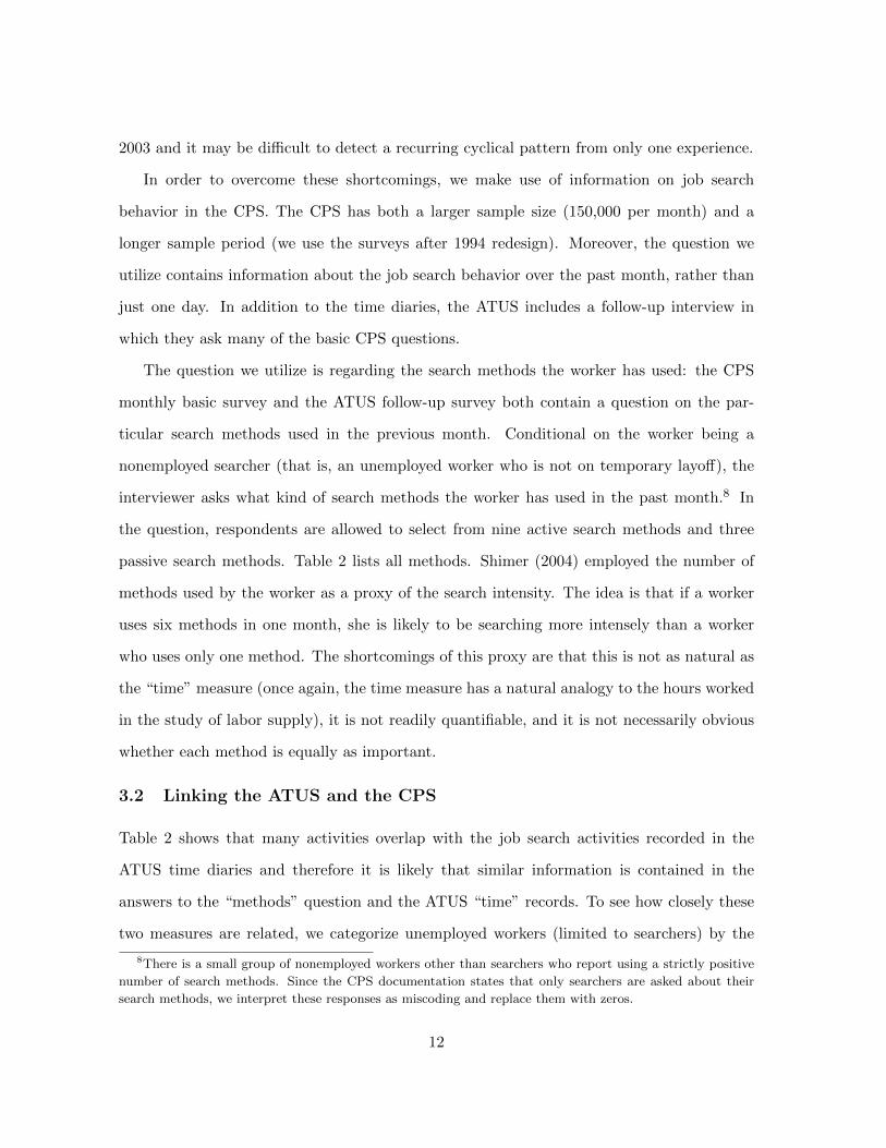
searching for a job). Here, we aim at determining the extensive margin by examining which
category of workers can be considered as active searchers. Table 3 reports the average time
(in minutes per day) spent on job search activities reported in the time diaries of the ATUS
for workers in each category of labor market state.
In addition to standard categorizations (employed and nonemployed; employed, unem-
ployed, and not in the labor force [NILF]), we divide unemployed workers into two cate-
gories (“temporary layoffs” and “searchers”) and non-participants into two categories (“non-
searchers” and “other NILF”).10 Searchers are defined to be the unemployed workers who
are not on temporary layoff, and non-searchers are the workers who are not in the labor
force but who report that they “want a job.”11 The sum of searchers and non-searchers are
categorized as “attached workers.”
Table 3 reveals large differences in search time among different categories. Not so sur-
prisingly, unemployed workers spend much more time searching for a job compared to either
employed workers or those not in the labor force. There is also some difference in search
time between workers on temporary layoff and searchers, but workers on temporary layoff do
10This classification, as well as the terminology of “searchers,” “non-searchers,” and “attached workers,”
follows Shimer (2004).11This is a larger category than “marginally attached workers”—a marginally attached worker has to be
available for working and have searched during the past 12 months (but not past four weeks), in addition to
reporting that she wants a job.
16
1994 1996 1998 2000 2002 2004 2006 2008 2010 2012
0.6
0.7
0.8
1994 1996 1998 2000 2002 2004 2006 2008 2010 2012
0.6
0.7
0.8
1994 1996 1998 2000 2002 2004 2006 2008 2010 20120.05
0.1
0.15
0.2
0.25
U
U + NS(left scale)
U
U + N(right scale)
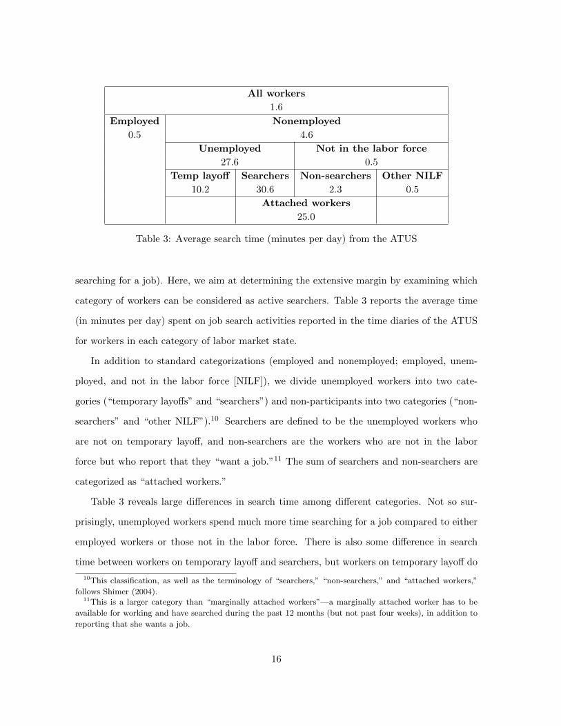
Figure 3: The time series of extensive margins: U/(U +N) and U/(U +NS)
spend significant time searching. Therefore, it is clear from Table 3 that the answer to “who
are actively searching?” is “the unemployed workers.” Thus in the next section we identify
the extensive margin of search by the unemployed workers.
4 Cyclicality of search effort
In this section, we describe how nonemployed workers’ search behavior has changed over
time. As we described above, we divide the search intensity into two margins: the extensive
margin and the intensive margin. Given that we will use the unemployed workers as the
extensive margin, our main departure from the DMP literature is the measurement of the
intensive margin.
4.1 The extensive margin
As we discussed in the previous section, the most reasonable answer to “who is search-
ing?” is “the unemployed workers.” Figure 3 plots the ratio of unemployed worker (U) to all
17

1994 1996 1998 2000 2002 2004 2006 2008 2010 2012
−0.05
0
0.05
0.1
0.15
0.2
U
U + N
U
U + NS
Figure 4: The time series of the time dummies µs. The sample population is U +N for the
dotted line and U +NS for the solid line.
nonemployed workers (N) and the ratio of unemployed workers to the sum of the number
of unemployed workers and the number of nonsearchers (NS).12 Here, the denominator is
meant to represent the “entire population of potential workers.” In the most general context,
it corresponds to the “entire population who are in the appropriate age range.”13 In that
case, the appropriate denominator is all nonemployed workers. Another reasonable choice is
to exclude workers who do not want to work, in which case the sum of unemployed workers
and the nonsearchers is the appropriate denominator.
Figure 3 clearly shows that the extensive margin is countercyclical. This is not a surpris-
ing observation given that the strong countercyclicality of unemployment has been widely
documented. In order to control for the changes in composition of the nonemployed pool over
the business cycle, we estimate a linear probability model that is similar to that in Shimer’s
12This sum corresponds to “generalized unemployment” in the language of Krusell et al. (2010).13In this paper, the age range is from 25 to 70.
18

(2004). We run the regression (using the U +N and U +NS sample)
yit = x′itδ +∑s
µsms + εit, (5)
where yit is 1 if i ∈ U and 0 if i /∈ U , xit is the same set of controls as in (4) with the
coefficient vector δ, and ms is the month dummy that takes 1 if s = t and 0 otherwise. Figure
3 plots the coefficients on the month dummy, µs, for each s. These coefficients provide an
estimate of how much being in a particular month raises the probability of being in U given
that you are not employed. Like Figure 3, this time series is also countercyclical.
Although the results on the extensive margin provide some useful information about
search effort decision, this is a rough measure of each worker’s search effort. In addition,
in the context of many search models, the extensive margin is effectively irrelevant, since
typically the “entire population of workers” is considered as employment plus unemployment.
Thus we examine the “intensive margin” in the next subsection.
4.2 The intensive margin
We use the imputed minutes, sit, calculated in Section 3.2, as our measure of search effort
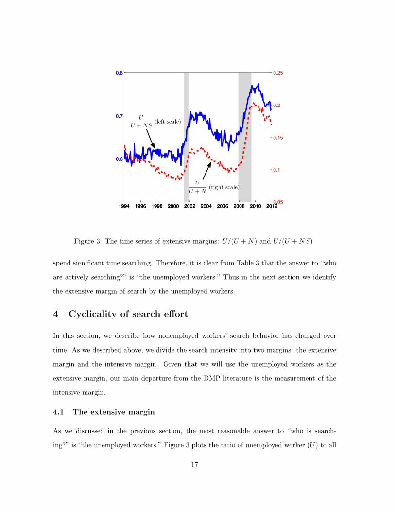
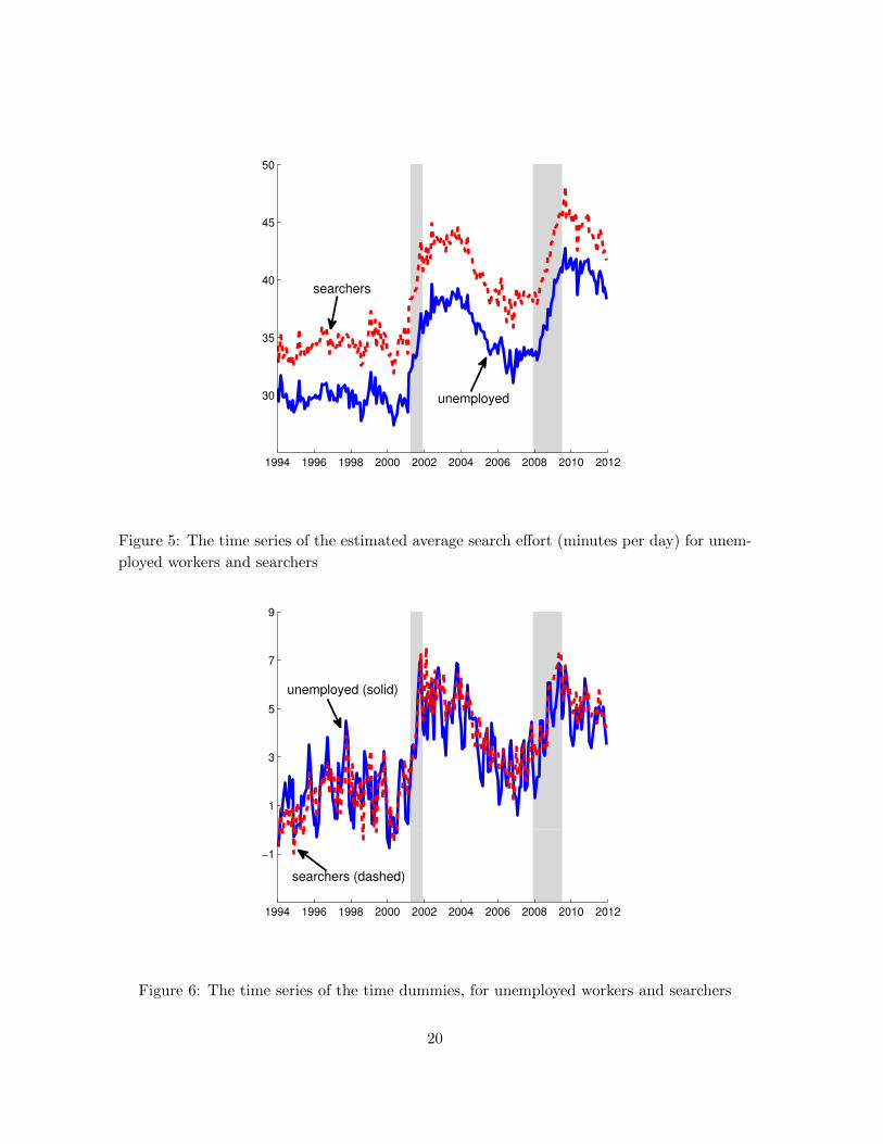
at the intensive margin. Figure 5 plots the time series of the average sit in minutes per day.
The solid line is the average minutes per day that an unemployed worker spends on search
activities and the dotted line is the corresponding number for searchers. They clearly also
exhibit a countercyclical pattern.
In order to see if the same pattern holds after controlling for the composition of unem-
ployed workers, we run a similar regression as (5) with sit for the unemployed worker on the
left-hand side. Figure 6 plots the coefficients on the month dummies and shows that the
countercyclical pattern remains even after controlling for observed changes in composition.
4.3 Total
The total search effort by nonemployed workers in the economy can be calculated as [the
fraction of unemployed in the population]×[intensive margin]. This is the counterpart of s
19
1994 1996 1998 2000 2002 2004 2006 2008 2010 2012
30
35
40
45
50
searchers
unemployed
Figure 5: The time series of the estimated average search effort (minutes per day) for unem-
ployed workers and searchers
1994 1996 1998 2000 2002 2004 2006 2008 2010 2012
−1
1
3
5
7
9
searchers (dashed)
unemployed (solid)
Figure 6: The time series of the time dummies, for unemployed workers and searchers
20
1994 1996 1998 2000 2002 2004 2006 2008 2010 2012
2
3
4
5
6
7
8
9
10
searchers only(dashed)
all nonemployed(dotted)
unemployed only (solid)
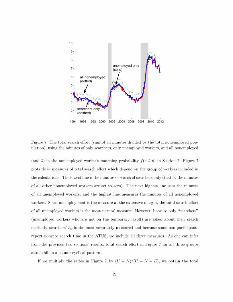
Figure 7: The total search effort (sum of all minutes divided by the total nonemployed pop-
ulation), using the minutes of only searchers, only unemployed workers, and all nonemployed
(and s) in the nonemployed worker’s matching probability f(s, s, θ) in Section 2. Figure 7
plots three measures of total search effort which depend on the group of workers included in
the calculations. The lowest line is the minutes of search of searchers only (that is, the minutes
of all other nonemployed workers are set to zero). The next highest line uses the minutes
of all unemployed workers, and the highest line measures the minutes of all nonemployed
workers. Since unemployment is the measure at the extensive margin, the total search effort
of all unemployed workers is the most natural measure. However, because only “searchers”
(unemployed workers who are not on the temporary layoff) are asked about their search
methods, searchers’ sit is the most accurately measured and because some non-participants
report nonzero search time in the ATUS, we include all three measures. As one can infer
from the previous two sections’ results, total search effort in Figure 7 for all three groups
also exhibits a countercyclical pattern.
If we multiply the series in Figure 7 by (U + N)/(U + N + E), we obtain the total
21

1994 1996 1998 2000 2002 2004 2006 2008 2010 2012
0.5
1
1.5
2
2.5
3
all nonemployed(dotted)
unemployed only (solid)
searchers only(dashed)
Figure 8: The total search effort (sum of all minutes divided by the total population), using
the minutes of only searchers, only unemployed workers, and all nonemployed
search effort in the economy. This is the natural counterpart of the input su in the matching
function M(su, v) in Section 2. These series are plotted in Figure 8 and again exhibit a
countercycical pattern.
4.4 Implications
Our result that the aggregate search effort by nonemployed workers is countercyclical has
several important implications for macroeconomic analysis of the labor market. Below we
discuss two of these.
4.4.1 Implications: driver of the aggregate labor market fluctuations
What does our result tell us about the source of cyclical fluctuation of the labor market?
The fact that workers are making more effort in searching for a job in recessions rules out the
possibility that labor supply is the sole determinant of the cyclical movement of employment
22
and unemployment—the employment decline in recessions is not because workers are not
looking for a job as hard as in booms.
Here, one has to be careful in making distinction between the cyclicality of aggregate effort
and individual effort. When workers are heterogeneous, it is possible that the aggregate
search effort is countercyclical while the individual effort is not. We have controlled for
the observable characteristics of the workers in the previous section, but the unobservable
characteristics may remain, as we will discuss further in Section 5.1.
However, for analyzing aggregate dynamics of the labor market, aggregate effort still pro-
vides useful information. In fact, Appendix C shows that, in the context of the DMP-style
model, the aggregate search effort has to be procyclical if aggregate employment and unem-
ployment are entirely supply-driven. This result casts doubts on the empirical plausibility of
a class of models whose employment dynamics is entirely supply-driven, such as Veracierto
(2008) and Christiano, Trabandt, and Walentin (2012).
4.4.2 Implications: matching function
Our observation that the intensive margin of search effort exhibit strong cyclicality has
important implications on the theoretical models that relies on the matching function. If we
consider only the number of unemployed workers as the input to the matching function as
in the standard DMP model, we are implicitly measuring the search effort only using the
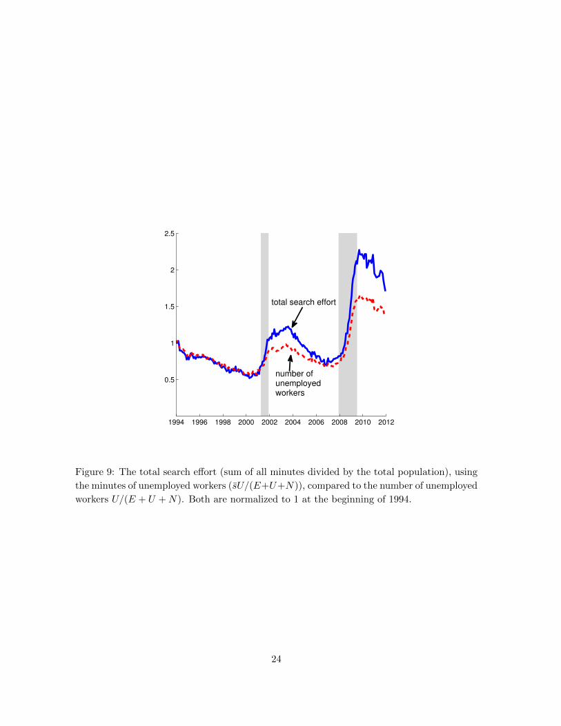
extensive margin. Figure 9 plots total search effort measures using only the extensive margin
(U/(E+U+N) against a measure that uses the intensive margin as well (sU/(E+U+N)),14
normalizing the initial levels to one. We see that, especially in recent years, the two lines
diverge significantly, illuminating the importance of appropriately taking the intensive margin
into account.
We can further measure the importance of the intensive margin by estimating the match-
ing function. Here, we consider simple linear regressions under the constant returns to scale
14Note that this is an appropriate input of the matching function in the context of (1) but may not be
appropriate in the context of (3).
23
1994 1996 1998 2000 2002 2004 2006 2008 2010 2012
0.5
1
1.5
2
2.5
total search effort
number ofunemployedworkers
Figure 9: The total search effort (sum of all minutes divided by the total population), using
the minutes of unemployed workers (sU/(E+U+N)), compared to the number of unemployed
workers U/(E + U +N). Both are normalized to 1 at the beginning of 1994.
24

assumption.15 There is a large literature on estimating matching functions (earlier literature
was surveyed by Petrongolo and Pissarides, 2001) but none have considered the worker’s
search intensity, except for Yashiv (2000).
We use the data from JOLTS and CPS from December 2000 to December 2011. The job
finding probability ft is obtained by dividing the “hires” variable in JOLTS by the number
of unemployed in CPS. The variable θt is obtained by dividing the “vacancy” variable in
JOLTS by the number of unemployed in CPS. We consider the formulation
ln(ft) = δ0 + δθ ln(θt) + δs ln(st) + δddt + τt + εt, (6)
where ft is the job-finding probability, θt ≡ vt/ut where vt is vacancy and ut is unemployment,
τt is the month dummy, and εt is the error term. st is the aggregate value for intensive margin
of search effort (for each unemployed worker), measured in Section 4.2. dt is a dummy variable
that takes one for t before July 2009—this is to control for a recent large decline in matching
efficiency.
Table 4 shows the results of a simple OLS regression of the form (6), with and without
ln(st). The first column is the conventional matching function estimation, and the result is
within the range of the OLS results in the literature—see, for example, Borowczyk-Martins,
Jolivet, and Postel-Vinay (2013). The second column adds our search intensity variable
estimated from CPS, s. As is expected by the theory, the coefficient of ln(s) is positive and
significant at 1% level. The inclusion of this variable also changes the estimated coefficient
of ln(θt) upwards.
As is argued by Borowczyk-Martins, Jolivet, and Postel-Vinay (2013), however, the OLS
estimate is likely biased. In particular, they argue that θt is endogenous in the conventional
matching function estimation when there are shocks to the matching efficiency. In our for-
mulation, their argument also can be applied to st. They devised a GMM estimation method
that is immune from this endogeneity bias. In particular, they assume that εt in (6) has an
ARMA structure and estimate the AR parameters εt together with the coefficients βi using
15See Appendix D for the interpretation in the context of the exact matching function in the form of (4).
25

Without ln(st) With ln(st)
ln(θt) 0.731∗∗∗ 0.831∗∗∗
(0.019) (0.036)
ln(st) − 0.522∗∗
− (0.164)
Table 4: Matching function estimation: OLS. Standard errors are in the parenthesis. ∗∗∗
indicates being significant at 0.1% level. ∗∗ indicates being significant at 1% level.
the lagged values of ln(θt) as instrumental variables. We extend their method to incorpo-
rate another endogenous variable ln(st). Following their method, we assume that εt follows
ARMA(3,3). We use ln(θt−i) and ln(st−i) where i = 4, 5, 6, 7, 8, 9 as the instrumental vari-
ables. (Note that here the system is over-identified.) Following Borowczyk-Martins, Jolivet,
and Postel-Vinay (2013), we repeat the estimation also with ln(ft−4) included in the list of
instrumental variables.
Lags of ln(θt) and ln(st) used as IV ln(ft) lag also included as IV
ln(θt) 0.793∗∗∗ 0.658∗∗∗
(0.143) (0.091)
ln(st) 0.055 −0.094
(0.436) (0.392)
Table 5: Matching function estimation: GMM method based on Borowczyk-Martins, Jo-
livet, and Postel-Vinay (2013). Standard errors are in the parenthesis. ∗∗∗ indicates being
significant at 0.1% level.
Table 5 shows the result. In both cases, the coefficient of ln(θt) is significant at 0.1%
significance level and also in line with the estimates in the previous studies (in Borowczyk-
Martins, Jolivet, and Postel-Vinay (2013), the corresponding numbers are 0.706 and 0.692).
The point estimates of both coefficients are lower than the OLS estimates, as the theory
would predict. Unfortunately, the coefficients of ln(s) have large standard errors and thus
cannot provide a conclusive evidence on the effect of st. We also experimented with adding
more instruments, including S&P-500 index and nation-wide house price index, but they did
not improve the estimates. This is because (i) the measurement of st is not as precise as θt
26
and (ii) the instruments are not very strong for st, and (iii) the negative externality among
workers may wash out the individual effect at the aggregate level. Further exploring this
issue and precisely identifying the sign and the magnitude of st coefficient is left for future
research.
In principle, the estimation of the matching function would also shed light on how the
worker’s effort and the firm’s effort are related technologically. In particular, as Appendix
D shows, (under the assumption of no externality in s) if the coefficient on the cross-term
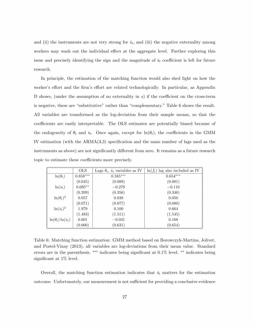
is negative, these are “substitutive” rather than “complementary.” Table 6 shows the result.
All variables are transformed as the log-deviation from their sample means, so that the
coefficients are easily interpretable. The OLS estimates are potentially biased because of
the endogeneity of θt and st. Once again, except for ln(θt), the coefficients in the GMM
IV estimation (with the ARMA(3,3) specification and the same number of lags used as the
instruments as above) are not significantly different from zero. It remains as a future research
topic to estimate these coefficients more precisely.
OLS Lags θt, st variables as IV ln(ft) lag also included as IV
ln(θt) 0.858∗∗∗ 0.585∗∗∗ 0.654∗∗∗
(0.045) (0.089) (0.081)
ln(st) 0.695∗∗ −0.279 −0.110
(0.209) (0.356) (0.346)
ln(θt)2 0.057 0.038 0.050
(0.071) (0.077) (0.080)
ln(st)2 1.979 0.100 0.664
(1.483) (1.511) (1.545)
ln(θt) ln(st) 0.601 −0.031 0.168
(0.660) (0.631) (0.654)
Table 6: Matching function estimation: GMM method based on Borowczyk-Martins, Jolivet,
and Postel-Vinay (2013), all variables are log-deviations from their mean value. Standard
errors are in the parenthesis. ∗∗∗ indicates being significant at 0.1% level. ∗∗ indicates being
significant at 1% level.
Overall, the matching function estimation indicates that st matters for the estimation
outcome. Unfortunately, our measurement is not sufficient for providing a conclusive evidence
27

on how it matters in the IV estimation, and a further examination is left for the future
research.
5 Why is the search effort countercyclical?
Our results in Section 4 indicate that the search effort is countercyclical, both at the in-
tensive and the extensive margins. This section makes several attempts to account for this
countercyclicality, especially in the intensive margin.
Note that, as is mentioned in the previous section and we will discuss further below,
unobserved heterogeneity is an important issue in the measurement of the cyclicality of the
intensive margin in the aggregate, since the pool of searchers change over time. We have
shown that aggregate search effort is countercyclical, and this holds for the intensive margin
as well. This observation is true even after controlling for observed heterogeneity. However,
in addition to changes in observed characteristics of searchers, there is a countercyclical bias
stemming from unobserved heterogeneity when we consider individual-level effort. We deal
with this issue of unobserved heterogeneity by exploiting the panel aspect of the CPS and find
that unobserved heterogeneity indeed has some effect on analyzing the response of individual
search effort to external environment.
5.1 The individual decision rules
In the context of our simple model in Section 2, job search behavior is strongly influenced
by either labor market conditions, θ, and present value of wealth, a.
Below, we run various individual-level regressions to uncover the factors that influence
individuals’ decision for s. The regression equation is
sit = θitδθ + witδw + x′itδx + εit, (7)
where θit is a measure of labor market conditions with δθ as the associated coefficient, wit
is the wealth variable with the associated coefficient δw, and xit is the vector of controls
and δx is the associated coefficient vector. εit is the error term. The controls include the
28

usual demographic controls (a quartic in age, marital status, race, sex, and education), four
occupation dummies,16 a quartic function of unemployment duration, and month dummies.
5.2 Individual response to aggregate condition
First, we run the individual-level regression (7), with the individual sit on the left-hand side,
and using the aggregate-level θt (we use the vacancy-unemployment ratio) and the aggregate-
level measure of wealth on the right-hand side. We restrict the sample to the searchers,
whose imputed time is based on the search methods used in addition to the individual
characteristics. Table 7 shows the regression results for equation (7) using two alternative
measures of aggregate labor market conditions and two alternative measures of wealth. The
two measures of labor market conditions come from the vacancy series in the JOLTS and
HWOL datasets, which we use to compute the aggregate labor market tightness (vacancy-
unemployment ratio) v/u. The JOLTS survey starts in 2001 and gives us a longer time
series while the HWOL series start in 2005. For wealth, we use S&P 500 and the aggregate
Core-Logic house price index. Full results of the regression are reported in Appendix E.
JOLTS HWOL
Market tightnesss (θ) −0.930∗∗∗ −1.098∗∗∗ −2.146∗∗∗ −2.857∗∗∗
(0.118) (0.118) (0.248) (0.336)
S&P 500 −0.005∗∗∗ − −0.003∗∗∗ −(0.001) − (0.001) −
House Price Index − −0.025∗∗∗ − -0.004
− (0.002) − (0.006)
Table 7: Regression results using aggregate measures of labor market tightness and wealth.
Standard errors are in the parenthesis. ∗∗∗ indicates being significant at 0.1% level. Full
regression results are reported in Appendix E Table 13.
Table 7 suggests that the searchers tend to reduce their search effort when aggregate
labor market conditions are favorable (that is, when θt is high). These results are consistent
with the matching function being “substitutive” rather than “complementary” between st
16We use the occupation categorization in Acemoglu and Autor (2011), in which occupations are divided
into four categories, cognitive/non-routine, cognitive/routine, manual/non-routine, and manual/routine.
29
and θt. We also find that workers search harder in periods where aggregate wealth measures
are low.
5.3 Individual response to local labor market condition
It is most likely that the labor-market condition θt for a particular individual is not the
aggregate-level θt but is determined within a more narrow labor market. Ideally, we would
like to see the effect of the labor market conditions that an individual faces in her job
search and her current level of wealth. Unfortunately, it is impossible to observe the labor
market conditions that an individual is facing in her job search for two reasons: (i) there
is no good information about the market that a particular individual is searching at in the
currently available data sources and (ii) computing labor market tightness requires knowing
the number of unemployed in very small markets—due to the small sample size of the CPS,
unemployment counts become unreliable for small labor markets making it impossible to
compute the corresponding labor market tightness. In addition, available data sources do
not provide us any information on individuals’ wealth.
What we do here is to run the regression (7) using several different measures of labor
market conditions and wealth. In particular, we use market tightness at the census region
and state level in order to capture more individual-specific labor markets and a state-level
house price index to get closer to personal wealth. In addition, we also try the interaction
of occupations and locations as the definition of the individuals’s labor market—specifically,
we define 4× 4 = 16 labor markets which are the interaction of four occupation categories17
and four Census regions.
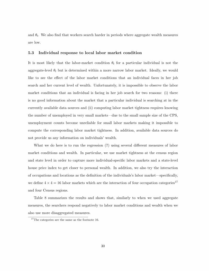
Table 8 summarizes the results and shows that, similarly to when we used aggregate
measures, the searchers respond negatively to labor market conditions and wealth when we
also use more disaggregated measures.
17The categories are the same as the footnote 16.
30
Census Region State Occupation×Region
Market tightnesss (θ) −1.121∗∗∗ −1.500∗∗∗ −0.339∗∗ −0.454∗∗ −1.122∗∗∗ −1.862∗∗
(0.113) (0.103) (0.124) (0.140) (0.181) (0.142)
S&P 500 −0.004∗∗∗ − −0.006∗∗∗ − −0.004∗∗∗ −(0.001) − (0.001) − (0.001) −
House Price Index − −0.017∗∗∗ − −0.018∗∗∗ − −0.015∗∗∗
− (0.002) − (0.002) − (0.002)
Table 8: Regression results using market-specific measures of labor market tightness and
wealth. The Census Region regressions use the JOLTS and the others are based on the
HWOL. Full regression results are reported in Appendix E Table 14.
5.4 The issue of unobserved heterogeneity
As we discussed earlier, an important issue is unobserved heterogeneity that could potentially
create a cyclical composition bias. For example, suppose that searchers are heterogeneous
in their desire to work and that a worker with a strong preference to work tends to make
higher search effort and tends to transit to employment more quickly than other workers.
In booms, workers tend to transit to employment more quickly, and “high search effort”
workers may disappear from the unemployment pool faster. As a result, during booms, the
unemployment pool would be dominated by workers with less desire to work. This channel
could create a countercyclical bias in the observed average effort per nonemployed through
composition changes.
To address this issue, we attempt to control for the desire to work in various ways. One
component of the unobserved heterogeneity that can affect the cyclicality of job search effort
is the individual’s labor market attachment, which is typically hard to observe and effects the
individual’s desire to work. We attempt to control for labor force attachment by following
Elsby, Hobijn, and Sahin (2012) who show that the composition of the unemployment pool
gets skewed towards workers who are more attached to the labor force during recessions. We
follow their analysis and use prior labor market status of unemployed workers as a proxy
for labor force attachment. To do this, we use the CPS microdata matched across all eight
survey months and only include people who were unemployed at some point in the 5th to
31
the 8th month in the survey and who we are able to match to their survey exactly one year
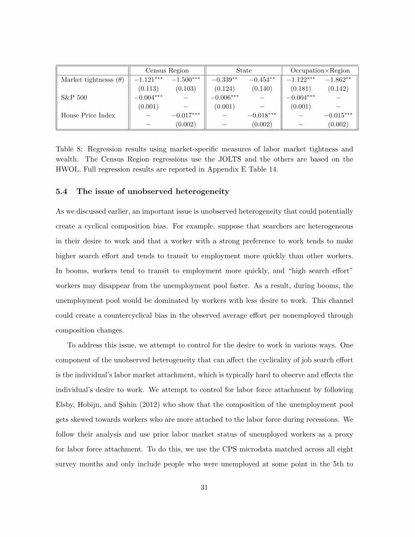
ago. We define their prior status as their labor market status 12 months ago. We find that
workers who were nonparticipants a year ago, and thus had the lowest degree of attachment,
have the lowest job search effort. Workers who were in the labor force a year ago search
harder, with those who were employed a year ago searching more intensity than those who
were unemployed. Table 9 shows that while job search effort still responds negatively to
better labor market conditions, prior employment status is an important determinant of job
search effort and that those with a stronger desire to work search more intensely.
JOLTS HWOL
Market Tightness −0.577∗∗∗ −0.924∗∗∗ −1.476∗∗∗ −3.574∗∗∗
(0.213) (0.214) (0.451) (0.607)
S & P 500 −0.005∗∗∗ − −0.004∗∗∗ −(0.001) − (0.001) −
House Price Index − −0.023∗∗∗ − 0.011
− (0.004) − (0.010)
Employed 1 year ago 6.015∗∗∗ 6.029∗∗∗ 5.975∗∗∗ 5.981∗∗∗
(0.216) (0.216) (0.271) (0.271)
Unemployed 1 year ago 4.918∗∗∗ 4.821∗∗∗ 4.910∗∗∗ 4.856∗∗∗
(0.255) (0.254) (0.306) (0.306)
Table 9: Regression results using aggregate measures of labor market tightness and wealth
with eligibility. Full regression results are reported in Appendix E Table 15.
As another attempt to control for the unobserved heterogeneity in desire to work, below
we exploit the full panel structure of the CPS and run regressions with individual fixed effects.
Assuming that an individual’s desire to work does not change over the sample period, this
some directly control for the unobserved compositional bias. When we control for individual
fixed effects, we only use the individuals with at least 2 periods of unemployment in the eight
months in which they are surveyed. In Tables 10 and 11, we report regression results with
fixed effects. Since this sample is smaller than the overall sample we used for the regressions
reported in Tables 7 and 8, we report the results without fixed effects for the same sample in
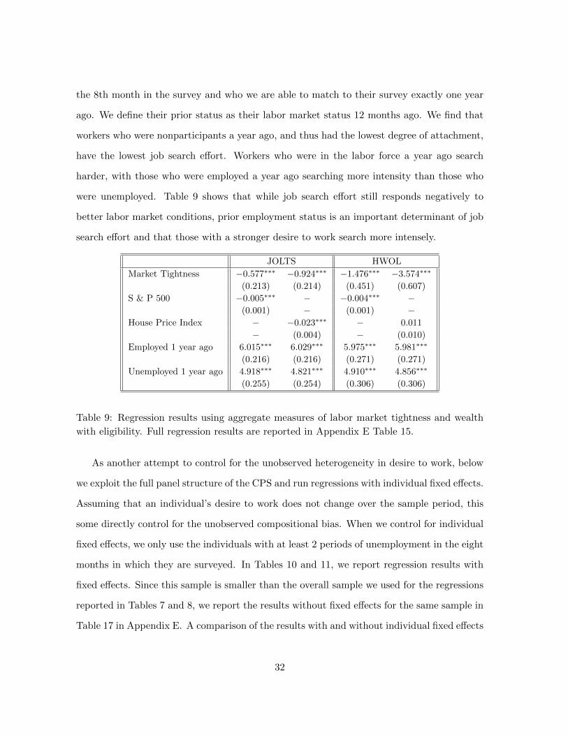
Table 17 in Appendix E. A comparison of the results with and without individual fixed effects
32
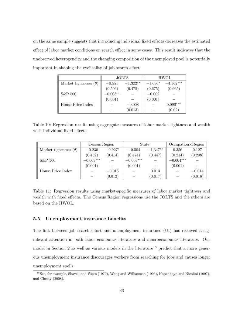
on the same sample suggests that introducing individual fixed effects decreases the estimated
effect of labor market conditions on search effect in some cases. This result indicates that the
unobserved heterogeneity and the changing composition of the unemployed pool is potentially
important in shaping the cyclicality of job search effort.
JOLTS HWOL
Market tightnesss (θ) −0.551 −1.322∗∗ −1.696∗ −4.362∗∗∗
(0.506) (0.475) (0.675) (0.665)
S&P 500 −0.003∗∗ − −0.002 −(0.001) − (0.001) −
House Price Index − −0.008 − 0.096∗∗∗
− (0.013) − (0.02)
Table 10: Regression results using aggregate measures of labor market tightness and wealth
with individual fixed effects.
Census Region State Occupation×Region
Market tightnesss (θ) −0.230 −0.927∗ −0.504 −1.347∗∗ 0.356 0.127
(0.452) (0.414) (0.474) (0.447) (0.214) (0.208)
S&P 500 −0.003∗∗∗ − −0.003∗∗∗ − −0.004∗∗∗ −(0.001) − (0.001) − (0.001) −
House Price Index − −0.015 − 0.013 − −0.014
− (0.012) − (0.017) − (0.016)
Table 11: Regression results using market-specific measures of labor market tightness and
wealth with fixed effects. The Census Region regressions use the JOLTS and the others are
based on the HWOL.
5.5 Unemployment insurance benefits
The link between job search effort and unemployment insurance (UI) has received a sig-
nificant attention in both labor economics literature and macroeconomics literature. Our
model in Section 2 as well as various models in the literature18 predict that a more gener-
ous unemployment insurance discourages workers from searching for jobs and causes longer
unemployment spells.
18See, for example, Shavell and Weiss (1979), Wang and Williamson (1996), Hopenhayn and Nicolini (1997),
and Chetty (2008).
33
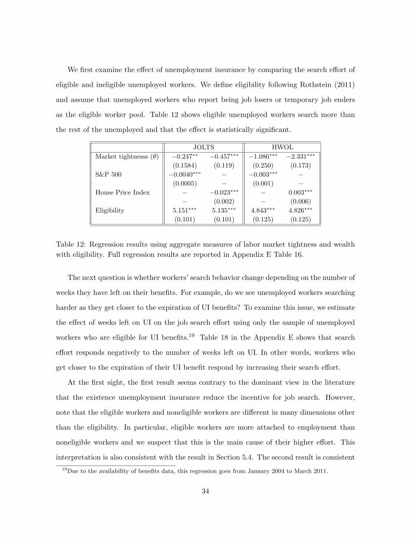
We first examine the effect of unemployment insurance by comparing the search effort of
eligible and ineligible unemployed workers. We define eligibility following Rothstein (2011)
and assume that unemployed workers who report being job losers or temporary job enders
as the eligible worker pool. Table 12 shows eligible unemployed workers search more than
the rest of the unemployed and that the effect is statistically significant.
JOLTS HWOL
Market tightnesss (θ) −0.247∗∗ −0.457∗∗∗ −1.086∗∗∗ −2.331∗∗∗
(0.1584) (0.119) (0.250) (0.173)
S&P 500 −0.0040∗∗∗ − −0.003∗∗∗ −(0.0005) − (0.001) −
House Price Index − −0.023∗∗∗ − 0.003∗∗∗
− (0.002) − (0.006)
Eligibility 5.151∗∗∗ 5.135∗∗∗ 4.843∗∗∗ 4.826∗∗∗
(0.101) (0.101) (0.125) (0.125)
Table 12: Regression results using aggregate measures of labor market tightness and wealth
with eligibility. Full regression results are reported in Appendix E Table 16.
The next question is whether workers’ search behavior change depending on the number of
weeks they have left on their benefits. For example, do we see unemployed workers searching
harder as they get closer to the expiration of UI benefits? To examine this issue, we estimate
the effect of weeks left on UI on the job search effort using only the sample of unemployed
workers who are eligible for UI benefits.19 Table 18 in the Appendix E shows that search
effort responds negatively to the number of weeks left on UI. In other words, workers who
get closer to the expiration of their UI benefit respond by increasing their search effort.
At the first sight, the first result seems contrary to the dominant view in the literature
that the existence unemployment insurance reduce the incentive for job search. However,
note that the eligible workers and noneligible workers are different in many dimensions other
than the eligibility. In particular, eligible workers are more attached to employment than
noneligible workers and we suspect that this is the main cause of their higher effort. This
interpretation is also consistent with the result in Section 5.4. The second result is consistent
19Due to the availability of benefits data, this regression goes from January 2004 to March 2011.
34
with the standard theory. As the unemployment duration lengthens during the recession,
this effect also contributes to the countercyclical aggregate search effort.
5.6 Taking stock
In this section, we have examined how individual search effort is affected by various factors.
As our model in Section 2 suggests, the wealth level has consistently negative effects in various
regressions. The labor market environment, represented by the vacancy-unemployment ratio,
tend to have negative a effect on search effort. This suggests that the job-finding technology
may be “substitutive” between individual search effort and the labor market condition. Thus
the elements that we highlighted in Section 2 indeed seem to contribute to the countercyclical
pattern of job search effort.
There is also an indication that unobserved heterogeneity is important. Workers who
are eligible for UI benefits incur more efforts than the noneligible workers, and the effort
level increases as the expiration date becomes closer. There are other controls that show
interesting relationship with the search effort—Appendix F highlights two examples, age and
unemployment duration.
6 Conclusion
This paper examined the cyclical pattern of job search effort by nonemployed workers. Our
innovation is to combine the information in ATUS and CPS in order to overcome the short-
comings of each dataset.
We found that the job search effort by nonemployed workers is countercyclical at the
aggregate level, in both extensive and intensive margin. This finding casts a doubt on the
validity of the models that relies entirely on worker’s search effort (the supply side of the labor
market) in explaining procyclical employment. This also implies that ignoring the intensive
margin in the matching function may quantitatively miss the fluctuation of the worker’s side
of the search input.
35

The individual-level regression found that a worker’s search effort negatively responds to
wealth, as is predicted by the model. The labor market condition tends to have a negative
effect on search as well. These results are suggestive in accounting for the countercyclical
aggregate search effort, but far from conclusive, given that we don’t have a good measure of
individual wealth and the information on how labor market is segmented. Further examina-
tion of the potential causes of the countercyclicality, as well as a further analysis on the role
of unobserved heterogeneity, is left for future research.
36
References
[1] Acemoglu, D. and D. Autor (2011). “Skills, Tasks and Technologies: Implications for
Employment and Earnings,” in D. Card and O. Ashenfelter (eds.) H andbook of Labor
Economics 4B, 1043-1171.
[2] Aguiar, M., E. Hurst, and L. Karabarbounis (2012). “Time Use during Recessions,”
forthcoming American Economic Review.
[3] Borowczyk-Martins, D., G. Jolivet, and F. Postel-Binay (2012). “Accounting for Endo-
geneity in Matching Function Estimation,” forthcoming Review of Economic Dynamics.
[4] Blanchard, O. J. and P. Diamond (1990). “The Cyclical Behavior of the Gross Flows of
U.S. Workers,” Brookings Papers on Economic Activity 21, 85-156.
[5] Chetty, R. (2008). “Moral Hazard versus Liquidity and Optimal Unemployment Insur-
ance,” Journal of Political Economy 116, 173–234.
[6] Christiano, L., M. Trabandt, and K. Walentin (2012). “Involuntary Unemployment and
the Business Cycle,” mimeo.
[7] DeLoach, S. B. and M. R. Kurt (2012). “Discouraging Workers: Estimating the Impacts
of Macroeconomic Shocks on the Search Intensity of the Unemployed,” mimeo.
[8] Davis, S. J., Faberman, R. J., and J.C. Haltiwanger (2010). “The Establishment-Level
Behavior of Vacancies and Hiring,” NBER Working Paper 16265.
[9] Elsby, M., B. Hobijn and A. Sahin (2012). “On the Importance of the Participation
Margin for Labor Market Fluctuations,” mimeo.
[10] Gomme, P. and D. Lkhagvasuren (2012). “The Cyclicality of Search Intensity in a Com-
petitive Search Model,” mimeo.
[11] Hopenhayn, H. A. and J. P. Nicolini (1997). “Optimal Unemployment Insurance,” Jour-
nal of Political Economy 105, 412-438.
37
[12] Kroft, K. and M. J. Notowidigdo (2011). “Should Unemployment Insurance Vary With
the Unemployment Rate? Theory and Evidence,” mimeo.
[13] Krueger, A. B., and A. Mueller (2010). “Job Search and Unemployment Insurance: New
Evidence from Time Use Data,” Journal of Public Economics, 94, 298-307.
[14] Krusell, P., T. Mukoyama, R. Rogerson, and A. Sahin (2010). “Aggregate Labor Market
Outcomes: The Roles of Choice and Chance,” Quantitative Economics 1, 97-127.
[15] Landais, C., P. Michaillat, and E. Saez (2011). “Optimal Unemployment Insurance over
the Business Cycle,” mimeo.
[16] Merz, M. (1995). “Search in the Labor Market and the Real Business Cycle,” Journal
of Monetary Economics 36, 269-300.
[17] Petrongolo, B. and C. A. Pissarides (2001). “Looking into the Black Box: A Survey of
the Matching Function,” Journal of Economic Literature 39, 390-431.
[18] Pissarides, C. A. (1985). “Short-Run Equilibrium Dynamics of Unemployment, Vancan-
cies, and Real Wages,” American Economic Review 75, 676-690.
[19] Pissarides, C. A. (2000). Equilibrium Unemployment Theory, Second Edition, MIT
Press, Cambridge.
[20] Rothstein, J. (2011). “Unemployment Insurance and Job Search in the Great Recession,”
Brookings Papers on Economic Activity, Fall 2011,143-210.
[21] Shavell, S. and L. Weiss (1979). “The Optimal Payment of Unemployment Insurance
Benefits over Time,” Journal of Political Economy 87, 1347-1362.
[22] Shimer R. (2004). “Search Intensity,” mimeo.
[23] Shimer, R. (2005). “The Cyclical Behavior of Equilibrium Unemployment and Vacan-
cies,” American Economic Review 95, 25-49.
38

[24] Shimer, R. (2011). “Job Search, Labor Force Participation, and Wage Rigidities,”
mimeo.
[25] Veracierto, M. (2008). “On the Cyclical Behavior of Employment, Unemployment and
Labor Force Participation,” Journal of Monetary Economics, 55, 1143-1157.
[26] Wang, C. and S. Williamson (1996). “Unemployment Insurance with Moral Hazard in
a Dynamic Economy,” Carnegie-Rochester Conference Series on Public Policy 44, 1-41.
[27] Yashiv, E. (2000). “The Determinants of Equilibrium Unemployment,” American Eco-
nomic Review 90, 1297-1322.
39

Appendix
A A general equilibrium search-matching model
This section presents an infinite-horizon general equilibrium model.
A.1 General setup
The aggregate number of matches at each period is dictated by the matching function
M(ut, vt; st), where st is the average search effort in the economy, vt is the aggregate va-
cancy, and ut is the number of unemployed workers at time t. At the individual level,
matching is stochastic, and the probability of worker i finding a job is f(sit, st, θt), where sit
is his search effort and θt ≡ vt/ut. The probability of a firm finding a worker is q(st, θt). The
separation probability of a matched job-worker pair is σ. The job-worker match produces zt
unit of consumption goods, and zt follows a Markov process.
A.1.1 Unemployment dynamics
The total population is 1, and therefore the number of employed workers is 1 − ut. The
dynamics of the unemployment is dictated by
ut+1 = σ(1− ut) + (1− f(sit, st, θt))ut. (8)
A.1.2 Value functions
Let the (aggregate) state variable at time t be St ≡ (ut, zt). From a firm’s perspective, the
value of being matched with a worker, J(St), is:
J(St) = zt − w(St) + βE[(1− σ)J(St+1) + σV (St+1)], (9)
where V (St) is the value of vacancy and w(St) is the wage paid to the worker. The expectation
E[·] is taken with the information of St. The value of vacancy is
V (St) = −κ+ βE[q(st, θt)J(St+1) + (1− q(st, θt))V (St+1)]. (10)
40

For the worker’s side, the value of being employed, W (St), is
W (St) = w(St) + βE[(1− σ)W (St+1) + σU(St+1)], (11)
and the value of being unemployed, U(St), is
U(St) = maxsit{b− c(sit) + βE[f(sit, st, θt)W (St+1) + (1− f(sit, st, θt))U(St+1)]} . (12)
The first-order condition for the right hand side is:
c′(sit) = βf1(sit, st, θt)E[W (St+1)− U(St+1)]. (13)
Denote sit that satisfies (13) by s∗it.
A.1.3 Wage determination
Let
J(w;St) = zt − w + βE[(1− σ)J(St+1) + σV (St+1)|St]
and
W (w;St) = w + βE[(1− σ)W (St+1) + σU(St+1)].
The wage is determined by the generalized Nash bargaining with the worker’s bargaining
power γ ∈ (0, 1). Then w solves
(1− γ)(W (w;St)− U(St)) = γ(J(w;St)− V (St)). (14)
A.1.4 Free entry and equilibrium
We assume free entry to vacancy posting, V (St) = 0. From (10),
κ = βq(st, θt)E[J(St+1)] (15)
holds, and (9) can be rewritten as
J(St) = zt − w(St) + β(1− σ)E[J(St+1)].
41

Therefore,
J(St) = zt − w(St) +(1− σ)κ
q(st, θt).
Using this to the right-hand side of (15) yields
κ = βq(st, θt)E
[zt+1 − w(St+1) +
(1− σ)κ
q(st+1, θt+1)
]. (16)
From (11) and (12),
W (St)− U(St) = w(St)− b+ c(s∗it) + βE[(1− σ − f(s∗it, st, θt))(W (St+1)− U(St+1))].
This can be rewritten as
w(St) = W (St)− U(St) + b− c(s∗it)− βE[(1− σ − f(s∗it, st, θt))(W (St+1)− U(St+1))].
From (14),
W (St)− U(St) =γ
1− γJ(St).
Thus
w(St) =γ
1− γJ(St) + b− c(s∗it)− β(1− σ − f(s∗it, st, θt))
γ
1− γE[J(St+1)].
Once again, from (15),
w(St) =γ
1− γJ(St) + b− c(s∗it)−
γ
1− γ(1− σ − f(s∗it, st, θt))κ
q(st, θt).
Forwarding one period, taking expectation, and using (15) once again,
E[w(St+1)] =γ
1− γκ
βq(st, θt)+ b− E[c(s∗i,t+1)]− γ
1− γE
[(1− σ − f(s∗i,t+1, st+1, θt+1))κ
q(st+1, θt+1)
].
(17)
Let us impose the equilibrium condition and denote st = s∗it = st. Then combining (16)
and (17) we obtain
κ
1− γ= βq(st, θt)E
[zt+1 − b+ c(st+1) +
1− σ − γf(st+1, st+1, θt+1)
1− γκ
q(st+1, θt+1)
]. (18)
42

The equation (13) can be rewritten as
c′(st) = f1(st, st, θt)γ
1− γκ
q(st, θt). (19)
Equations (18) and (19) determine the dynamics of θt and st. Note that the variable u
do not appear in both (18) and (19). This implies that the dynamics of θt and st (both jump
variables) are not influenced by u (only influenced by z). Once we know the dynamics of θt
and st from (18) and (19), we can determine the dynamics of unemployment by (8) and u0.
A.2 Pissarides (1985) model (no effort choice)
A special case is when st is constant, which boils down to the standard Pissarides (1985)
model. This case is easy to analyze. Assume that f(θ) = χθ1−η and q(θ) = χθ−η, where
χ > 0 and η ∈ (0, 1). Then, log-linearizing (18) around the steady-state yields (the “tilde”
(˜) denotes the value at the steady state and the “hat” (ˆ) denotes the log deviation from
the steady state)
Aθt = E[zzt+1 + Bθt+1],
where A ≡ κηθη/(1− γ)βχ and B ≡ [(1− σ)κηθη/(1− γ)χ]− [γκθ/(1− γ)].
Assume that zt+1 = ρzt + εt+1, where ρ ∈ (0, 1) and εt+1 is a mean zero random variable
(thus z = 1). Since the equilibrium θ has to take the form
θt = Czt,
using the method of undetermined coefficients,
C =ρ
A− ρB=
1− γ
κθη([
1
ρβ− (1− σ)
]η
χ+ γθ1−η
) . (20)
This makes it clear that, for example, for given θ the amplification (C) is large when κ is small.
This is the background of Hagedorn and Manovskii’s (2008) main result. (In order to keep θ
and other parameters constant, a small κ requires a large value of b.) This analytical result
43

that C is increasing in ρ appears new in the literature.20 If we normalize C by multiplying√1− ρ2 so that the unconditional variance of the shock is constant, a sufficient condition
for this coefficient being increasing in ρ will become (1− σ)η > γχθ1−η.
A.3 Pissarides (2000, Ch 5) model
Now, let’s go back to the original model, with (18) and (19). Assume that c(s) = φsω/ω,
where ω > 1. As in Pissarides (2000, Ch 5), assume that the matching function takes the
form of M(su, v) and the worker’s job finding rate is f(s, s, θ) = sM(1, θ/s). In particular,
assume a Cobb-Douglas function for the matching function:
M(su, v) = χ(su)ηv1−η,
where χ > 0 and η ∈ (0, 1). The worker’s job finding probability is
f(s, s, θ) = χs
(θ
s
)1−η.
The probability of a vacancy finding a worker is
q(s, θ) = χsηθ−η.
The equation (18) is now
κ
1− γ= βχsηt θ
−ηt E
[zt+1 − b+
φ
ωsωt+1 +
1− σ − γχsηt+1θ1−ηt+1
1− γκ
χsηt+1θ−ηt+1
].
Rearranging, this can be rewritten as
κ
(1− γ)βχs−ηt θηt = E
[zt+1 − b+
φ
ωsωt+1 +
(1− σ)κ
(1− γ)χs−ηt+1θ
ηt+1 −
γκ
1− γθt+1
].
Log-linearizing this yields
κs−η θηη
(1− γ)βχ(θt − st) = E
[zzt+1 + φsω st+1 +
(1− σ)κs−η θηη
(1− γ)χ(θt+1 − st+1)− γκθ
1− γθt+1
].
(21)
20Most of the papers which characterize the analytical properties of the DMP model rely on the steady-state
comparison, which makes it impossible to analyze the effect of ρ. Hornstein, Krusell, and Violante (2005)
analyze a stochastic model, but with the shock taking only two points.
44

The equation (19) can be rewritten as
φsω−1t =
γκ
1− γθtst. (22)
This can be solved as
st =
(γκ
(1− γ)φθt
) 1ω
.
Log-linearizing,
st =1
ωθt. (23)
This makes it clear that st responds positively to θt. This is no surprise given our results in
the simple model. There is no effect of wealth given the linear utility and b stays constant.
The job finding probability is complementary between s and θ, which tends to make s move
in the same direction as θ. The effect of wage enhances it, since the wage also tends to be
procyclical. It responds less when the curvature of the effort cost function (ω) is larger.
Using (23), (21) can be rewritten as
Aθt = E[zzt+1 + Bθt+1],
using the same assumption on z as before and following the same steps (we used the fact
that (22) also holds in the steady state), we obtain
θt = Czt,
where
C =ω
ω − 1
1− γ
κθη([
1
ρβ− (1− σ)
]η
χsη+ γθ1−η
) .This is remarkably similar to (20). The only differences are (i) χ is now replaced by χsη,
since now this is the “effective” match efficiency on average, and (ii) the term ω/(ω − 1) is
multiplied in front, since the movement of s influences the cyclical movement of the prob-
ability of a vacancy finding a worker, changing the incentive for vacancy posting. There is
a “magnification” (when χsη is replaced by χ), since ω/(ω − 1) > 1. This was observed by
Merz (1995) and Gomme and Lkhagvasuren (2011) in related, numericaly-solved models.
45

A.4 A model with “substitutive” matching function
Now assume that
M(s, u, v) = χ
(αsψ + (1− α)
(vu
)ψ)ηu
and
f(s, s, θ) = χ(αsψ + (1− α)θψ)η,
where χ > 0, α ∈ (0, 1),η ∈ (0, 1), ψ > 0, and ψη < 1. Note that this is a special case of (3).
It follows that
q(s, θ) = χ(αsψ + (1− α)θψ)ηθ−1.
Note that f13 < 0 is satisfied in this formulation.
The equation (18) can be rearranged to
κ
(1− γ)βχ(αsψt + (1− α)θψt )−ηθt
= E
[zt+1 − b+
φ
ωsωt+1 +
(1− σ)κ
(1− γ)χ(αsψt+1 + (1− α)θψt+1)−ηθt+1 −
γκ
1− γθt+1
](24)
and the equation (19) is21
φsω−1t =
αηγκψ
1− γsψ−1t θt
αsψt + (1− α)θψt.
Rearranging and log-linearizing, we obtain
st =αsψ − (ψ − 1)(1− α)θψ
ωαsψ + (ω − ψ)(1− α)θψθt. (25)
Denote the right-hand side as Ξθt. Similarly to (23), the absolute value of Ξ is small when
ω is large. In contrast to (23), here s can react negatively to θ (i.e. Ξ > 0) if ψ is sufficiently
large (or α is sufficiently small). Note that f13 < 0 is not sufficient for this because the effect
from wage still exists.
21We also have to check the second-order condition in this case, because the concavity of f in s is not
necessarily guaranteed. It is
φ(ω − 1)sω−2t − γκηψαsψ−2
t θt
(1− γ)(αsψt + (1− α)θψt )
((ψ − 1) +
ψ(η − 1)αsψ
αsψt + (1− α)θψt
)> 0.
46

Log-linearizing (24) and using (25), we obtain the equation
Aθt = E[zzt+1 + Bθt+1],
where
A =κ
(1− γ)βχ(αsψ + (1− α)θψ)−η θ
[1− ηαψs
ψΞ + (1− α)ψθψ
αsψ + (1− α)θψ
]and
B =κ
1− γ
(1− σχ
(αsψ + (1− α)θψ)−η θ
[1− ηαψs
ψΞ + (1− α)ψθψ
αsψ + (1− α)θψ
]− γθ
)+ φsωΞ.
As before, this can be solved as
θt =ρ
A− ρBzt.
Below we solve this numerically. Several parameter values are given upfront: set ω = 4,
α = 0.1, ψ = 2, and η = 0.3. One period is assumed to be one month: thus set β = 0.98713
and ρ = 0.9513 (both from Cooley and Prescott (1995)). Following Shimer (2005), set γ = 0.72
and σ = 0.034. Let θ = 1 and s = 1 in the steady state (later these will pin down κ and φ).
Set χ so that the steady-state job finding rate χ(αsψ + (1− α)θψ)η = χ(0.1 + 0.9)0.3 = 0.45.
We set the value of nonemployment, b − φsω/ω = b − φ/4 = 0.7, along the line of Hall and
Milgrom (2008). κ and φ are set from the steady-state version of (18) and (19).
The resulting parameter values are χ = 0.45, φ = 0.0161, b = 0.708, and κ = 0.104. The
movement of endogenous variables are governed by
st = −0.3636θt
and
θt = 3.3750zt.
Thus in this case st reacts negatively to the change in θt (and therefore zt).
47

B More details on imputation
Let Yit be the search time we observe in ATUS for worker i at time t. What we are interested
in is not Yit per se—Yit contains one day’s sample from the search activities in entire period
t (one month), and we are interested in the entire month’s activity. Denote the “average”
search time over the month as E[Yit]. Let Pit be the probability that i searches strictly
positive minutes at the ATUS survey date in period t. Let Mit be the minutes that i searches
at the survey date of time t, conditional on searching strictly positive minutes. Then the
“average” minutes, E[Yit], is
E[Yit] = Pr[Yit > 0]E[Yit|Yit > 0] + Pr[Yit = 0]E[Yit|Yit = 0] = PitE[Mit]
from the law of iterated expectations.
Our purpose is to obtain E[Yit] for every CPS sample, but unfortunately we do not observe
it, we estimate it from the observed characteristics, including the the search methods she used.
We estimate E[Yit] based on the characteristics Xit (denote the estimate as EX [E[Yit]]). From
the above equation,
EX [E[Yit]] = EX [PitE[Mit]] = EX [Pit]EX [E[Mit]] + covX(Pit, E[Mit]),
holds, where EX [·] denotes the expected value conditional on X and covX(·, ·) denotes the
covariance conditional on X. We assume that covX(Pit, E[Mit]) = 0. Then
EX [E[Yit]] = EX [Pit]EX [E[Mit]].
This provides us the following two-step strategy for estimating EX [E[Yit]]
1. In order to obtain EX [Pit] for the CPS sample,
(a) Generate {0, 1} dummy variable (call yit) based on the minutes value of ATUS
sample (zero if the minutes is zero, one if it is strictly positive).
(b) Run a probit regression with this dummy variable on the left-hand side and the
characteristics of the corresponding ATUS sample on the right-hand side. More
48

specifically, maximize the log-likelihood
ln(L) =∑i,t
(yit ln Φ(x′itβ) + (1− yit) ln(1− Φ(x′itβ))),
where xit is the vector of Xit, to obtain the estimated values of β, β.
(c) Use the estimated coefficients above and the characteristics of the CPS sample to
calculate the predicted value of Pit for the CPS sample. More specifically,
EX [Pit] = Φ(x′itβ).
2. In order to obtain EX [E[Mit]] for the CPS sample,
(a) Use the subset of the ATUS sample who reports strictly positive minutes. Let
minutes be Qit.
(b) Run the regression
ln(Qit) = γ0 + γ1X1,it + ...+ γnXn,it + ε
for the ATUS sample, where ε is assumed to be mean zero normal with variance
σ2.
(c) Then, for the CPS sample, obtain
EX [E[Mit]] = exp
(γ0 + γ1X1,it + ...+ γnXn,it +
σ2
2
)from the property of the lognormal distribution, where σ2 is the estimated value
of σ2.
3. In order to obtain EX [E[Yit]] for the CPS sample, multiply EX [Pit] and EX [E[Mit]]
calculated above.
Through this method, we are able to impute a strictly positive amount of search time
for all non-employed in both the ATUS and CPS given their reported search methods and
observables. Importantly, in addition to including dummies for for each of the twelve search
49

methods, xit contains two sets of observables. The first is a set of worker characteristics which
may affect the intensity of their job search. We mostly follow Shimer (2004) in the choice of
these controls and include a quartic of age (ageit) and dummies for education levels (educ1it
for high school diploma, educ2it for some college, and educ3it for college plus), race (blackit),
gender (femaleit), and marital status (marriedit). We also add the interaction term of
femaleit and marriedit since being married is likely to affect the labor market behavior of
men and women differentially. The second set or controls are for labor market status. These
controls are intended to capture the search time for the respondents who do not answer the
CPS question on job search methods but still report positive search time. Here, we include
a dummy for being out of the labor force but not wanting a job (otherNILFit), being on
temporary layoff (layoffit), and being a out of the labor force but wanting a job (NSit).
C Implications of countercylical search effort
This section shows that our evidence goes against a model where the cyclical movement of
employment and unemployment are entirely supply-driven. We show that the observed total
search effort of such an economy is procyclical.
Consider of an infinite-horizon model with continuum of workers, who are either em-
ployed or nonemployed. Workers are heterogeneous and each selects a search effort s when
nonemployed. Suppose that the job-finding probability is an increasing function of s: f(s).
Employment is purely driven by this search effort, so that s is the only factor that affects the
job-finding probability. The separation probability is the same across workers and constant
over time (as in Pissarides (1985)) at δ.
Below we compare the steady states of a “good state” and “bad state”. In the U.S.
economy, the job-finding probability is sufficiently large so that the cyclical movement is
well-approximated by steady state comparisons (see, for example, Shimer (2005)). Below, we
assume that f ′(s)s/f(s) ≤ 1 (if we consider f(s) = sζ , this means that ζ ≤ 1).
From the above assumptions, the steady-state probability of a worker with search effort s
50

being nonemployed is δ/(f(s)+δ). Suppose that s is distributed across the entire population
with the distribution function G(s). Then the steady-state nonemployment rate in the entire
economy is ∫δ
f(s) + δdG(s) (26)
and the observed total search effort by nonemployed workers is∫s
δ
f(s) + δdG(s). (27)
Suppose that in a boom, G(s) increases in the sense of the first-order stochastic domi-
nance. Then the nonemployment rate (26) falls in the boom and the observed total effort
(27) rises. The first is straightforward from the fact that δ/(f(s) + δ) is decreasing in s.
The second is because sδ/(f(s) + δ) is increasing in s when f ′(s)s/f(s) ≤ 1. The effort per
nonemployed worker is ∫s
δ
f(s) + δdG(s)
/∫δ
f(s) + δdG(s)
and this is even more procyclical. Thus we established that, in this model, both total effort
of the nonemployed and the effort per nonemployed worker have to be procyclical even under
the presence of (unobserved) worker heterogeneity.
D Matching function estimation
This section establishes the link between the matching function estimations in Section 4.4.2
and the shape of the actual matching function. Recall that we consider the matching function
(restating (4))
M(s, u, v) = χ
(αsψ + (1− α)
(vu
)ψ)ηu.
The average job finding probability for each person in u is (slightly abusing the notation)
f(s, θ) = χ(αsψ + (1− α)θψ
)η.
When we run a linear regression
ln(ft) = δ0 + δs ln(st) + δθ ln(θt) + εt,
51
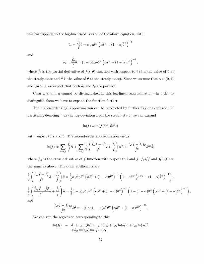
this corresponds to the log-linearized version of the above equation, with
δs =fs
fs = αψηsψ
(αsψ + (1− α)θψ
)−1
and
δθ =fθ
fθ = (1− α)ψηθψ
(αsψ + (1− α)θψ
)−1,
where fi is the partial derivative of f(s, θ) function with respect to i (s is the value of s at
the steady-state and θ is the value of θ at the steady-state). Since we assume that α ∈ (0, 1)
and ψη > 0, we expect that both δs and δθ are positive.
Clearly, ψ and η cannot be distinguished in this log-linear approximation—in order to
distinguish them we have to expand the function further.
The higher-order (log) approximation can be conducted by further Taylor expansion. In
particular, denoting ˆ as the log-deviation from the steady-state, we can expand
ln(f) = ln(f(ses, θeθ))
with respect to s and θ. The second-order approximation yields
ln(f) ≈∑i=s,θ
fi
fii+
∑i=s,θ
1
2
(fiif − f2
i
f2i+
fi
f
)ii2 +
fsθf − fsfθf2
sθsθ,
where fij is the cross derivative of f function with respect to i and j. fss/f and fθθ/f are
the same as above. The other coefficients are:
1
2
(fssf − f2
s
f2s+
fs
f
)s =
1
2αψ2ηsψ
(αsψ + (1− α)θψ
)−1(
1− αsψ(αsψ + (1− α)θψ
)−1),
1
2
(fθθf − f2
θ
F 2θ +
fθ
f
)θ =
1
2(1−α)ψ2ηθψ
(αsψ + (1− α)θψ
)−1(
1− (1− α)θψ(αsψ + (1− α)θψ
)−1),
and
fsθf − fsfθf2
sθ = −ψ2ηα(1− α)sψθψ(αsψ + (1− α)θψ
)−2.
We can run the regression corresponding to this:
ln(ft) = δ0 + δθ ln(θt) + δs ln(st) + δθθ ln(θt)2 + δss ln(st)
2
+δsθ ln(skt) ln(θt) + εt.
52

The most important coefficient is δsθ. In order to have “substitutability” between s and θ in
the job finding rate, η has to be positive, which implies δsθ < 0. Note that the correspondence
between δsθ and f13(s, s, θ) is warranted only when there is no externality coming from other
worker’s effort—that is, ξ = 0 in the context of (3). The variable ξ cannot be estimated from
the aggregate data.
E Additional results for individual regressions
The following tables show the additional results for the individual regressions.
53
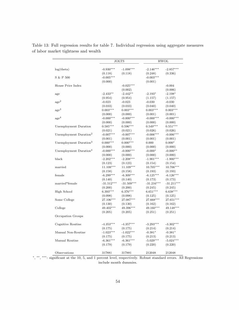
Table 13: Full regression results for table 7. Individual regression using aggregate measures
of labor market tightness and wealth
JOLTS HWOL
log(theta) -0.930∗∗∗ -1.098∗∗∗ -2.146∗∗∗ -2.857∗∗∗
(0.118) (0.118) (0.248) (0.336)
S & P 500 -0.005∗∗∗ -0.003∗∗∗
(0.000) (0.001)
House Price Index -0.025∗∗∗ -0.004
(0.002) (0.006)
age -2.433∗∗ -2.442∗∗ -2.193∗ -2.198∗
(0.954) (0.954) (1.157) (1.157)
age2 -0.023 -0.023 -0.030 -0.030
(0.033) (0.033) (0.040) (0.040)
age3 0.003∗∗∗ 0.003∗∗∗ 0.003∗∗∗ 0.003∗∗∗
(0.000) (0.000) (0.001) (0.001)
age4 -0.000∗∗∗ -0.000∗∗∗ -0.000∗∗∗ -0.000∗∗∗
(0.000) (0.000) (0.000) (0.000)
Unemployment Duration 0.585∗∗∗ 0.596∗∗∗ 0.549∗∗∗ 0.551∗∗∗
(0.021) (0.021) (0.026) (0.026)
Unemployment Duration2 -0.007∗∗∗ -0.007∗∗∗ -0.006∗∗∗ -0.006∗∗∗
(0.001) (0.001) (0.001) (0.001)
Unemployment Duration3 0.000∗∗∗ 0.000∗∗∗ 0.000 0.000∗
(0.000) (0.000) (0.000) (0.000)
Unemployment Duration4 -0.000∗∗∗ -0.000∗∗∗ -0.000∗ -0.000∗∗
(0.000) (0.000) (0.000) (0.000)
black -2.202∗∗∗ -2.208∗∗∗ -1.901∗∗∗ -1.900∗∗∗
(0.123) (0.123) (0.154) (0.154)
married 11.108∗∗∗ 11.109∗∗∗ 10.705∗∗∗ 10.706∗∗∗
(0.158) (0.158) (0.193) (0.193)
female -6.299∗∗∗ -6.309∗∗∗ -6.125∗∗∗ -6.126∗∗∗
(0.140) (0.140) (0.173) (0.173)
married*female -31.512∗∗∗ -31.509∗∗∗ -31.216∗∗∗ -31.211∗∗∗
(0.200) (0.200) (0.245) (0.245)
High School 6.393∗∗∗ 6.376∗∗∗ 6.651∗∗∗ 6.638∗∗∗
(0.098) (0.098) (0.125) (0.125)
Some College 27.106∗∗∗ 27.087∗∗∗ 27.668∗∗∗ 27.651∗∗∗
(0.130) (0.130) (0.162) (0.162)
College 49.402∗∗∗ 49.396∗∗∗ 49.160∗∗∗ 49.148∗∗∗
(0.205) (0.205) (0.251) (0.251)
Occupation Groups
Cognitive Routine -4.353∗∗∗ -4.357∗∗∗ -3.293∗∗∗ -3.302∗∗∗
(0.175) (0.175) (0.214) (0.214)
Manual Non-Routine -1.023∗∗∗ -1.022∗∗∗ -0.381∗ -0.381∗
(0.175) (0.175) (0.213) (0.213)
Manual Routine -6.361∗∗∗ -6.361∗∗∗ -5.029∗∗∗ -5.024∗∗∗
(0.179) (0.179) (0.220) (0.220)
Observations 317881 317881 212048 212048∗, ∗∗, ∗∗∗: significant at the 10, 5, and 1 percent level, respectively. Robust standard errors. All Regressions
include month dummies.
54
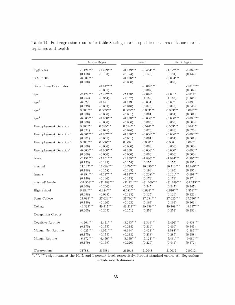
Table 14: Full regression results for table 8 using market-specific measures of labor market
tightness and wealth
Census Region State OccXRegion
log(theta) -1.121∗∗∗ -1.499∗∗∗ -0.339∗∗∗ -0.454∗∗∗ -1.122∗∗∗ -1.862∗∗∗
(0.113) (0.103) (0.124) (0.140) (0.181) (0.142)
S & P 500 -0.004∗∗∗ -0.006∗∗∗ -0.004∗∗∗
(0.000) (0.000) (0.000)
State House Price Index -0.017∗∗∗ -0.018∗∗∗ -0.015∗∗∗
(0.001) (0.002) (0.002)
age -2.474∗∗∗ -2.492∗∗∗ -2.120∗ -2.076∗ -2.001∗ -2.014∗
(0.954) (0.954) (1.157) (1.158) (1.165) (1.165)
age2 -0.022 -0.021 -0.033 -0.034 -0.037 -0.036
(0.033) (0.033) (0.040) (0.040) (0.040) (0.040)
age3 0.003∗∗∗ 0.003∗∗∗ 0.003∗∗∗ 0.003∗∗∗ 0.003∗∗∗ 0.003∗∗∗
(0.000) (0.000) (0.001) (0.001) (0.001) (0.001)
age4 -0.000∗∗∗ -0.000∗∗∗ -0.000∗∗∗ -0.000∗∗∗ -0.000∗∗∗ -0.000∗∗∗
(0.000) (0.000) (0.000) (0.000) (0.000) (0.000)
Unemployment Duration 0.584∗∗∗ 0.595∗∗∗ 0.554∗∗∗ 0.576∗∗∗ 0.553∗∗∗ 0.561∗∗∗
(0.021) (0.021) (0.026) (0.026) (0.026) (0.026)
Unemployment Duration2 -0.007∗∗∗ -0.007∗∗∗ -0.006∗∗∗ -0.006∗∗∗ -0.006∗∗∗ -0.006∗∗∗
(0.001) (0.001) (0.001) (0.001) (0.001) (0.001)
Unemployment Duration3 0.000∗∗∗ 0.000∗∗∗ 0.000 0.000∗∗ 0.000 0.000∗
(0.000) (0.000) (0.000) (0.000) (0.000) (0.000)
Unemployment Duration4 -0.000∗∗∗ -0.000∗∗∗ -0.000 -0.000∗∗ -0.000∗ -0.000∗∗
(0.000) (0.000) (0.000) (0.000) (0.000) (0.000)
black -2.151∗∗∗ -2.101∗∗∗ -1.909∗∗∗ -1.880∗∗∗ -1.994∗∗∗ -1.995∗∗∗
(0.123) (0.123) (0.154) (0.155) (0.155) (0.155)
married 11.107∗∗∗ 11.088∗∗∗ 10.705∗∗∗ 10.690∗∗∗ 10.713∗∗∗ 10.689∗∗∗
(0.158) (0.158) (0.193) (0.193) (0.195) (0.195)
female -6.294∗∗∗ -6.327∗∗∗ -6.147∗∗∗ -6.208∗∗∗ -6.161∗∗∗ -6.197∗∗∗
(0.140) (0.140) (0.173) (0.173) (0.174) (0.174)
married*female -31.509∗∗∗ -31.489∗∗∗ -31.224∗∗∗ -31.200∗∗∗ -31.299∗∗∗ -31.275∗∗∗
(0.200) (0.200) (0.245) (0.245) (0.247) (0.247)
High School 6.384∗∗∗ 6.324∗∗∗ 6.681∗∗∗ 6.624∗∗∗ 6.616∗∗∗ 6.553∗∗∗
(0.098) (0.099) (0.125) (0.125) (0.126) (0.126)
Some College 27.085∗∗∗ 27.024∗∗∗ 27.706∗∗∗ 27.654∗∗∗ 27.625∗∗∗ 27.570∗∗∗
(0.130) (0.130) (0.162) (0.162) (0.163) (0.163)
College 49.392∗∗∗ 49.417∗∗∗ 49.211∗∗∗ 49.258∗∗∗ 49.108∗∗∗ 49.127∗∗∗
(0.205) (0.205) (0.251) (0.252) (0.252) (0.252)
Occupation Groups
Cognitive Routine -4.364∗∗∗ -4.421∗∗∗ -3.293∗∗∗ -3.349∗∗∗ -5.476∗∗∗ -6.938∗∗∗
(0.175) (0.175) (0.214) (0.214) (0.410) (0.345)
Manual Non-Routine -1.025∗∗∗ -1.051∗∗∗ -0.394∗ -0.423∗∗ -1.584∗∗∗ -2.385∗∗∗
(0.175) (0.175) (0.213) (0.213) (0.285) (0.258)
Manual Routine -6.372∗∗∗ -6.450∗∗∗ -5.050∗∗∗ -5.124∗∗∗ -7.431∗∗∗ -9.089∗∗∗
(0.179) (0.179) (0.220) (0.220) (0.444) (0.372)
Observations 317881 317881 212048 212048 210012 210012∗, ∗∗, ∗∗∗: significant at the 10, 5, and 1 percent level, respectively. Robust standard errors. All Regressions
include month dummies.
55

Table 15: Full regression results for table 9. Regression includes aggregate market tightness
and wealth.
JOLTS HWOL
log(theta) -0.577∗∗∗ -0.924∗∗∗ -1.476∗∗∗ -3.574∗∗∗
(0.213) (0.214) (0.451) (0.607)
Employed 1 year ago 6.015∗∗∗ 6.029∗∗∗ 5.975∗∗∗ 5.981∗∗∗
(0.216) (0.216) (0.271) (0.271)
Unemployed 1 year ago 4.918∗∗∗ 4.821∗∗∗ 4.910∗∗∗ 4.856∗∗∗
(0.255) (0.254) (0.306) (0.306)
S & P 500 -0.005∗∗∗ -0.004∗∗∗
(0.001) (0.001)
House Price Index -0.023∗∗∗ 0.011
(0.004) (0.010)
age -7.565∗∗∗ -7.422∗∗∗ -4.388∗∗ -4.375∗∗
(1.736) (1.737) (2.109) (2.109)
age2 0.154∗∗ 0.149∗∗ 0.047 0.047
(0.060) (0.060) (0.073) (0.073)
age3 -0.000 0.000 0.002 0.002
(0.001) (0.001) (0.001) (0.001)
age4 -0.000∗∗∗ -0.000∗∗∗ -0.000∗∗∗ -0.000∗∗∗
(0.000) (0.000) (0.000) (0.000)
Unemployment Duration 0.573∗∗∗ 0.586∗∗∗ 0.530∗∗∗ 0.533∗∗∗
(0.039) (0.039) (0.048) (0.048)
Unemployment Duration2 -0.006∗∗∗ -0.007∗∗∗ -0.005∗∗ -0.005∗∗
(0.002) (0.002) (0.002) (0.002)
Unemployment Duration3 0.000 0.000∗ 0.000 0.000
(0.000) (0.000) (0.000) (0.000)
Unemployment Duration4 -0.000 -0.000∗∗ -0.000 -0.000
(0.000) (0.000) (0.000) (0.000)
black -2.437∗∗∗ -2.453∗∗∗ -1.933∗∗∗ -1.934∗∗∗
(0.231) (0.231) (0.292) (0.292)
married 11.542∗∗∗ 11.541∗∗∗ 11.220∗∗∗ 11.220∗∗∗
(0.282) (0.282) (0.342) (0.342)
female -5.619∗∗∗ -5.637∗∗∗ -5.485∗∗∗ -5.484∗∗∗
(0.263) (0.264) (0.324) (0.324)
married*female -31.902∗∗∗ -31.896∗∗∗ -31.521∗∗∗ -31.509∗∗∗
(0.355) (0.355) (0.435) (0.435)
High School 6.260∗∗∗ 6.234∗∗∗ 6.689∗∗∗ 6.675∗∗∗
(0.183) (0.183) (0.230) (0.230)
Some College 26.696∗∗∗ 26.672∗∗∗ 27.534∗∗∗ 27.520∗∗∗
(0.234) (0.234) (0.290) (0.290)
College 50.040∗∗∗ 50.020∗∗∗ 49.992∗∗∗ 49.981∗∗∗
(0.361) (0.362) (0.443) (0.443)
Occupation Groups
Cognitive Routine -3.693∗∗∗ -3.719∗∗∗ -2.330∗∗∗ -2.332∗∗∗
(0.315) (0.315) (0.385) (0.385)
Manual Non-Routine -1.049∗∗∗ -1.066∗∗∗ -0.143 -0.148
(0.308) (0.309) (0.376) (0.376)
Manual Routine -6.087∗∗∗ -6.101∗∗∗ -4.241∗∗∗ -4.233∗∗∗
(0.318) (0.319) (0.392) (0.392)
Observations 103016 103016 68950 68950∗, ∗∗, ∗∗∗: significant at the 10, 5, and 1 percent level, respectively. Robust standard errors. All Regressions
include month dummies.
56
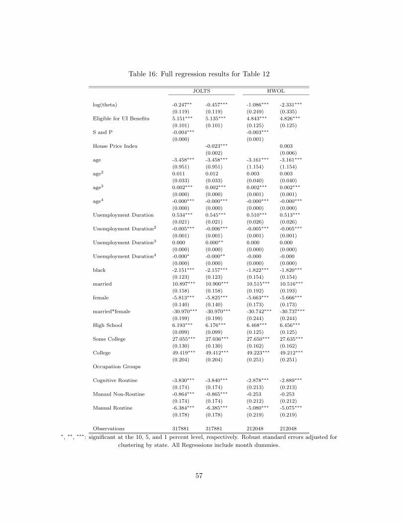
Table 16: Full regression results for Table 12
JOLTS HWOL
log(theta) -0.247∗∗ -0.457∗∗∗ -1.086∗∗∗ -2.331∗∗∗
(0.119) (0.119) (0.249) (0.335)
Eligible for UI Benefits 5.151∗∗∗ 5.135∗∗∗ 4.843∗∗∗ 4.826∗∗∗
(0.101) (0.101) (0.125) (0.125)
S and P -0.004∗∗∗ -0.003∗∗∗
(0.000) (0.001)
House Price Index -0.023∗∗∗ 0.003
(0.002) (0.006)
age -3.458∗∗∗ -3.458∗∗∗ -3.161∗∗∗ -3.161∗∗∗
(0.951) (0.951) (1.154) (1.154)
age2 0.011 0.012 0.003 0.003
(0.033) (0.033) (0.040) (0.040)
age3 0.002∗∗∗ 0.002∗∗∗ 0.002∗∗∗ 0.002∗∗∗
(0.000) (0.000) (0.001) (0.001)
age4 -0.000∗∗∗ -0.000∗∗∗ -0.000∗∗∗ -0.000∗∗∗
(0.000) (0.000) (0.000) (0.000)
Unemployment Duration 0.534∗∗∗ 0.545∗∗∗ 0.510∗∗∗ 0.513∗∗∗
(0.021) (0.021) (0.026) (0.026)
Unemployment Duration2 -0.005∗∗∗ -0.006∗∗∗ -0.005∗∗∗ -0.005∗∗∗
(0.001) (0.001) (0.001) (0.001)
Unemployment Duration3 0.000 0.000∗∗ 0.000 0.000
(0.000) (0.000) (0.000) (0.000)
Unemployment Duration4 -0.000∗ -0.000∗∗ -0.000 -0.000
(0.000) (0.000) (0.000) (0.000)
black -2.151∗∗∗ -2.157∗∗∗ -1.822∗∗∗ -1.820∗∗∗
(0.123) (0.123) (0.154) (0.154)
married 10.897∗∗∗ 10.900∗∗∗ 10.515∗∗∗ 10.516∗∗∗
(0.158) (0.158) (0.192) (0.193)
female -5.813∗∗∗ -5.825∗∗∗ -5.663∗∗∗ -5.666∗∗∗
(0.140) (0.140) (0.173) (0.173)
married*female -30.970∗∗∗ -30.970∗∗∗ -30.742∗∗∗ -30.737∗∗∗
(0.199) (0.199) (0.244) (0.244)
High School 6.193∗∗∗ 6.176∗∗∗ 6.468∗∗∗ 6.456∗∗∗
(0.099) (0.099) (0.125) (0.125)
Some College 27.055∗∗∗ 27.036∗∗∗ 27.650∗∗∗ 27.635∗∗∗
(0.130) (0.130) (0.162) (0.162)
College 49.419∗∗∗ 49.412∗∗∗ 49.223∗∗∗ 49.212∗∗∗
(0.204) (0.204) (0.251) (0.251)
Occupation Groups
Cognitive Routine -3.830∗∗∗ -3.840∗∗∗ -2.878∗∗∗ -2.889∗∗∗
(0.174) (0.174) (0.213) (0.213)
Manaul Non-Routine -0.864∗∗∗ -0.865∗∗∗ -0.253 -0.253
(0.174) (0.174) (0.212) (0.212)
Manual Routine -6.384∗∗∗ -6.385∗∗∗ -5.080∗∗∗ -5.075∗∗∗
(0.178) (0.178) (0.219) (0.219)
Observations 317881 317881 212048 212048∗, ∗∗, ∗∗∗: significant at the 10, 5, and 1 percent level, respectively. Robust standard errors adjusted for
clustering by state. All Regressions include month dummies.
57
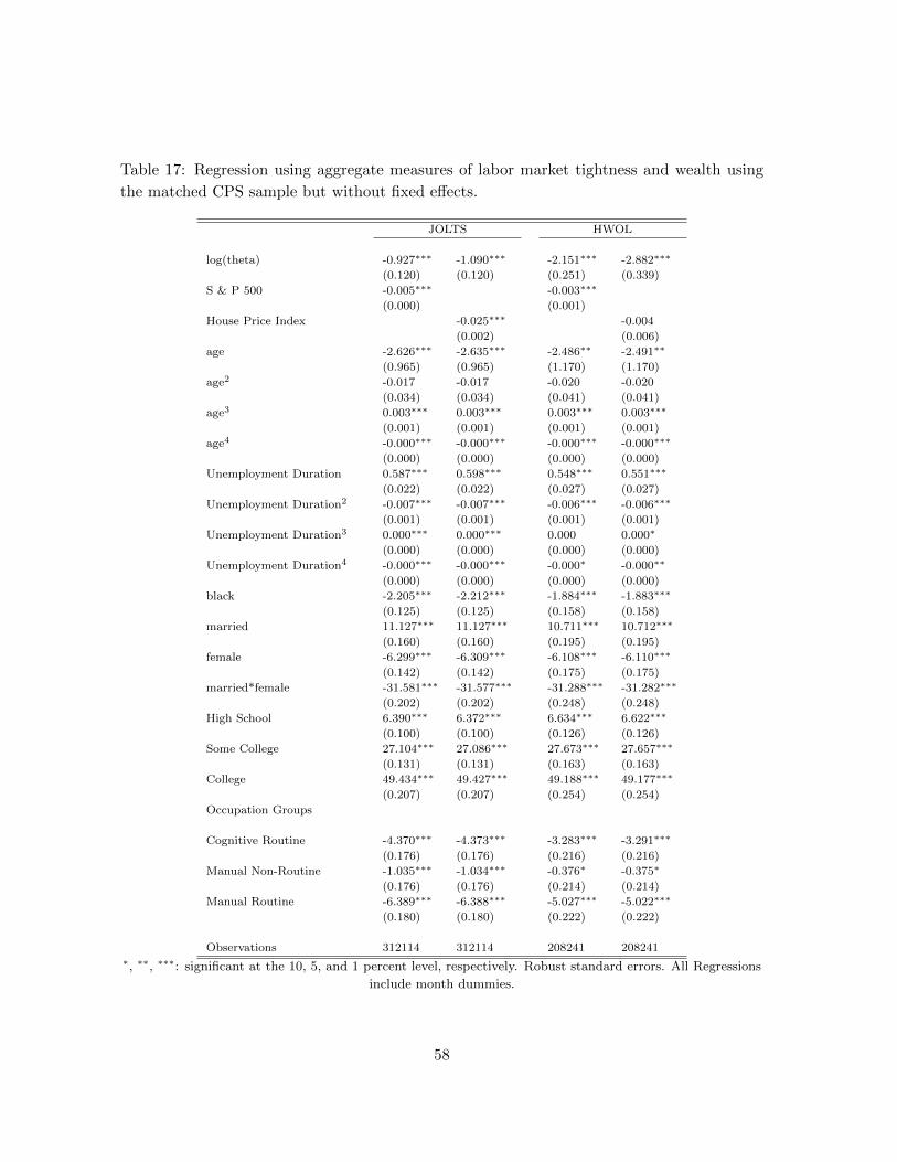
Table 17: Regression using aggregate measures of labor market tightness and wealth using
the matched CPS sample but without fixed effects.
JOLTS HWOL
log(theta) -0.927∗∗∗ -1.090∗∗∗ -2.151∗∗∗ -2.882∗∗∗
(0.120) (0.120) (0.251) (0.339)
S & P 500 -0.005∗∗∗ -0.003∗∗∗
(0.000) (0.001)
House Price Index -0.025∗∗∗ -0.004
(0.002) (0.006)
age -2.626∗∗∗ -2.635∗∗∗ -2.486∗∗ -2.491∗∗
(0.965) (0.965) (1.170) (1.170)
age2 -0.017 -0.017 -0.020 -0.020
(0.034) (0.034) (0.041) (0.041)
age3 0.003∗∗∗ 0.003∗∗∗ 0.003∗∗∗ 0.003∗∗∗
(0.001) (0.001) (0.001) (0.001)
age4 -0.000∗∗∗ -0.000∗∗∗ -0.000∗∗∗ -0.000∗∗∗
(0.000) (0.000) (0.000) (0.000)
Unemployment Duration 0.587∗∗∗ 0.598∗∗∗ 0.548∗∗∗ 0.551∗∗∗
(0.022) (0.022) (0.027) (0.027)
Unemployment Duration2 -0.007∗∗∗ -0.007∗∗∗ -0.006∗∗∗ -0.006∗∗∗
(0.001) (0.001) (0.001) (0.001)
Unemployment Duration3 0.000∗∗∗ 0.000∗∗∗ 0.000 0.000∗
(0.000) (0.000) (0.000) (0.000)
Unemployment Duration4 -0.000∗∗∗ -0.000∗∗∗ -0.000∗ -0.000∗∗
(0.000) (0.000) (0.000) (0.000)
black -2.205∗∗∗ -2.212∗∗∗ -1.884∗∗∗ -1.883∗∗∗
(0.125) (0.125) (0.158) (0.158)
married 11.127∗∗∗ 11.127∗∗∗ 10.711∗∗∗ 10.712∗∗∗
(0.160) (0.160) (0.195) (0.195)
female -6.299∗∗∗ -6.309∗∗∗ -6.108∗∗∗ -6.110∗∗∗
(0.142) (0.142) (0.175) (0.175)
married*female -31.581∗∗∗ -31.577∗∗∗ -31.288∗∗∗ -31.282∗∗∗
(0.202) (0.202) (0.248) (0.248)
High School 6.390∗∗∗ 6.372∗∗∗ 6.634∗∗∗ 6.622∗∗∗
(0.100) (0.100) (0.126) (0.126)
Some College 27.104∗∗∗ 27.086∗∗∗ 27.673∗∗∗ 27.657∗∗∗
(0.131) (0.131) (0.163) (0.163)
College 49.434∗∗∗ 49.427∗∗∗ 49.188∗∗∗ 49.177∗∗∗
(0.207) (0.207) (0.254) (0.254)
Occupation Groups
Cognitive Routine -4.370∗∗∗ -4.373∗∗∗ -3.283∗∗∗ -3.291∗∗∗
(0.176) (0.176) (0.216) (0.216)
Manual Non-Routine -1.035∗∗∗ -1.034∗∗∗ -0.376∗ -0.375∗
(0.176) (0.176) (0.214) (0.214)
Manual Routine -6.389∗∗∗ -6.388∗∗∗ -5.027∗∗∗ -5.022∗∗∗
(0.180) (0.180) (0.222) (0.222)
Observations 312114 312114 208241 208241∗, ∗∗, ∗∗∗: significant at the 10, 5, and 1 percent level, respectively. Robust standard errors. All Regressions
include month dummies.
58

Table 18: Regression controlling for weeks remaining on benefits. Included in the regression
are only eligible workers in the months in which there is benefits information. Aggregate
measures of markets conditions and wealth
JOLTS HWOL
log(theta) -8.978∗∗∗ -6.417∗∗∗
(0.376) (0.232)
Weeks of Benefits Remaining -0.119∗∗∗ -0.148∗∗∗
(0.006) (0.006)
S and P 0.003∗∗∗ 0.001
(0.001) (0.001)
House Price Index
age -0.703 -0.934
(1.750) (1.628)
age2 -0.100 -0.092
(0.061) (0.057)
age3 0.004∗∗∗ 0.004∗∗∗
(0.001) (0.001)
age4 -0.000∗∗∗ -0.000∗∗∗
(0.000) (0.000)
black -2.037∗∗∗ -2.326∗∗∗
(0.227) (0.207)
married 10.935∗∗∗ 11.178∗∗∗
(0.252) (0.235)
female -5.616∗∗∗ -5.566∗∗∗
(0.255) (0.234)
married*female -32.440∗∗∗ -32.698∗∗∗
(0.348) (0.322)
High School 7.615∗∗∗ 7.383∗∗∗
(0.181) (0.166)
Some College 29.977∗∗∗ 29.698∗∗∗
(0.241) (0.222)
College 54.004∗∗∗ 54.024∗∗∗
(0.373) (0.344)
Occupation Groups
Cognitive Routine -4.873∗∗∗ -5.281∗∗∗
(0.322) (0.298)
Manaul Non-Routine -1.330∗∗∗ -1.576∗∗∗
(0.314) (0.292)
Manual Routine -6.664∗∗∗ -7.167∗∗∗
(0.315) (0.291)
Observations 114494 132751∗, ∗∗, ∗∗∗: significant at the 10, 5, and 1 percent level, respectively. Robust standard errors adjusted for
clustering by state. All Regressions include month dummies.
59

F Other Determinants of Individual Job Search Effort
F.1 Demographic Characteristics
In our regressions we control for various demographic characteristics that generally affect
the labor market behavior of individuals. We find that the effects of these characteristics on
search intensity are robust to various specifications.
25 30 35 40 45 50 55 60 65 70
−1.2
−1
−0.8
−0.6
−0.4
−0.2
0
0.2
age
Figure 10: The effect of age on search time. These estimates from the regression in Table 7
column 1 and the first entry is normalized to 0.
F.2 Duration of Unemployment
The duration of unemployment is often considered an important determinant of job search
effort. In many models, agents’ search effort respond to their unemployment duration but
the direction of the change varies from model to model. One possibility is that as the
unemployment spell progresses, an unemployed worker’s savings become depleted, leading
the worker to search harder. However, various other forces can reverse this effect and move
job search time in the opposite direction over the unemployment spell. One example is human
60
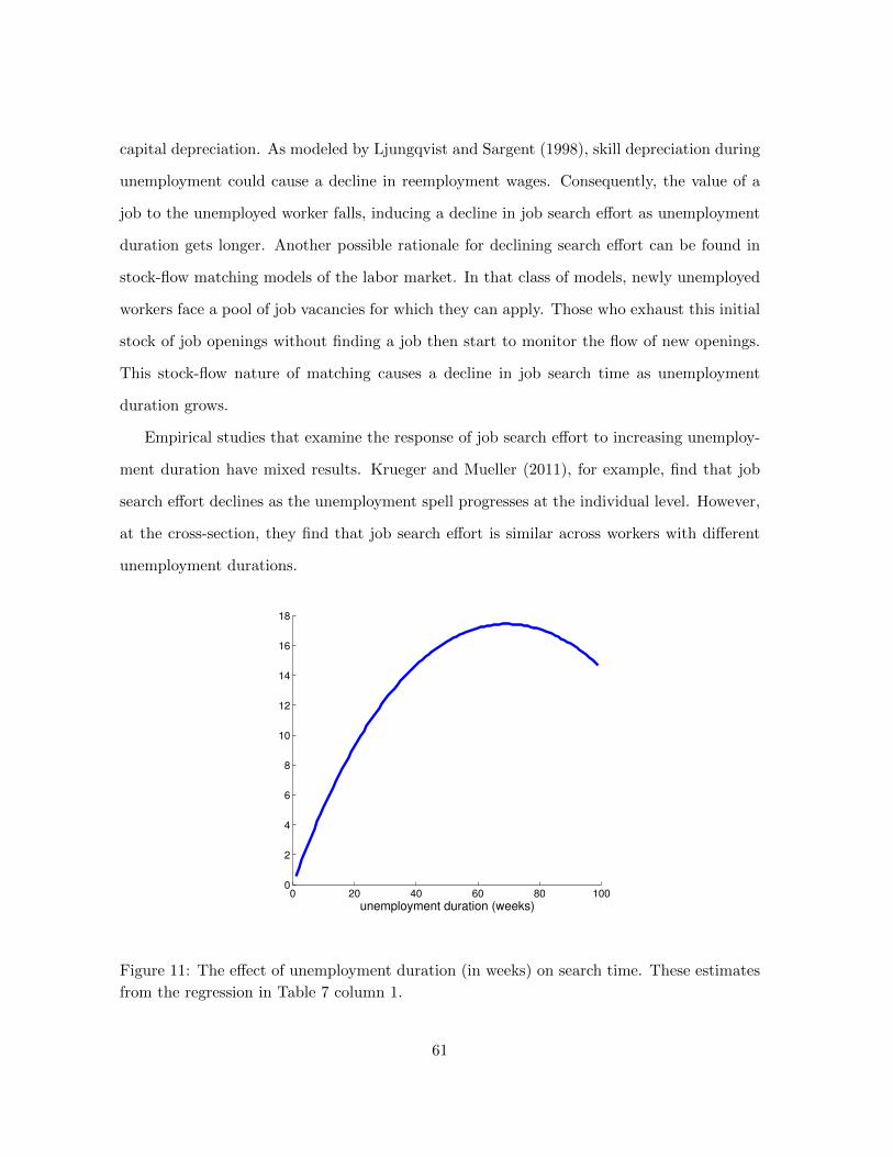
capital depreciation. As modeled by Ljungqvist and Sargent (1998), skill depreciation during
unemployment could cause a decline in reemployment wages. Consequently, the value of a
job to the unemployed worker falls, inducing a decline in job search effort as unemployment
duration gets longer. Another possible rationale for declining search effort can be found in
stock-flow matching models of the labor market. In that class of models, newly unemployed
workers face a pool of job vacancies for which they can apply. Those who exhaust this initial
stock of job openings without finding a job then start to monitor the flow of new openings.
This stock-flow nature of matching causes a decline in job search time as unemployment
duration grows.
Empirical studies that examine the response of job search effort to increasing unemploy-
ment duration have mixed results. Krueger and Mueller (2011), for example, find that job
search effort declines as the unemployment spell progresses at the individual level. However,
at the cross-section, they find that job search effort is similar across workers with different
unemployment durations.
0 20 40 60 80 1000
2
4
6
8
10
12
14
16
18
unemployment duration (weeks)
Figure 11: The effect of unemployment duration (in weeks) on search time. These estimates
from the regression in Table 7 column 1.
61

In our regressions we include a quartic function of unemployment duration following
Shimer (2004). Figure 11 shows that the response of search intensity to unemployment
duration in hump shaped, similar to Shimer’s findings. Search effort initially rises with
unemployment duration and then goes down. With the quartic specification, search effort
peaks after a year. We also try cubic and quintic polynomials and find that, while the other
coefficients of the regressions are robust to the degree of the polynomial in unemployment
duration, the peak of the polynomial changes, consistent with Shimer (2004).
62

Additional References for Appendix
[1] Cooley, T. F. and E. C. Prescott (1995). “Economic Growth and Business Cycles,” in Coo-
ley, T. F. ed. Frontiers of Business Cycle Research, Princeton University Press, Princeton.
[2] Hagedorn, M. and I. Manovskii (2008). “The Cyclical Behavior of Equilibrium Unem-
ployment and Vacancies Revisited,” American Economic Review 98, 1692-1706.
[3] Hall, R. E. and P. R. Milgrom (2008). “The Limited Influence of Unemployment on the
Wage Bargain,” American Economic Review 98, 1653-1674.
[4] Hornstein, A., P. Krusell, and G. L. Violante (2005). “Unemployment and Vacancy Fluc-
tuations in the Matching Model: Inspecting the Mechanism,” Federal Reserve Bank of
Richmond Economic Quarterly, 91, 19-50.
[5] Krueger, A. B. and A. Mueller, “Job Search, Emotional Well-Being and Job Finding in
a Period of Mass Unemployment: Evidence from High-Frequency Longitudinal Data”
Brookings Papers on Economic Activity 42, Spring 2011, 1-81.
[6] Ljungqvist, L. and T. Sargent (1998). “The European Unemployment Dilemma,” Journal
of Political Economy 106, 514-550.
63