Joni VirtaA I 577

ANNALES UNIVERSITATIS TURKUENSIS

Joni Virta

INDEPENDENT COMPONENT ANALYSIS FOR NON-STANDARD

DATA STRUCTURES

TURUN YLIOPISTON JULKAISUJA – ANNALES UNIVERSITATIS TURKUENSISSarja – ser. AI osa – tom. 577 | Astronomica – Chemica – Physica – Mathematica | Turku 2018

ISBN 978-951-29-7148-0 (PRINT)ISBN 978-951-29-7149-7 (PDF)

ISSN 0082-7002 (PRINT) | ISSN 2343-3175 (PDF)

Pain

osala

ma O

y, Tu

rku

, Fin

land

2018

TURUN YLIOPISTON JULKAISUJA – ANNALES UNIVERSITATIS TURKUENSISSarja - ser. A I osa - tom. 577 | Astronomica - Chemica - Physica - Mathematica | Turku 2018

Joni Virta

INDEPENDENT COMPONENT ANALYSIS FOR NON-STANDARD

DATA STRUCTURES

Supervised by

Professor Hannu OjaDepartment of Mathematics and StatisticsUniversity of Turku, Turku, Finland

Assistant Professor Klaus NordhausenCSTAT - Computational StatisticsInstitute of Statistics & Mathematical Methods in EconomicsVienna University of Technology, Vienna, Austria

Professor Bing LiDepartment of StatisticsPennsylvania State University, State College, PA, USA

University of Turku

Faculty of Science and EngineeringDepartment of Mathematics and StatisticsDoctoral Programme in Mathematics and Computer Sciences

Reviewed by

Professor Tõnu KolloInstitute of Mathematics and StatisticsUniversity of Tartu, Tartu, Estonia

Associate Professor Lexin LiDivision of Biostatistics University of California, Berkeley, CA, USA

The originality of this thesis has been checked in accordance with the University of Turku quality assurance system using the Turnitin OriginalityCheck service.

ISBN 978-951-29-7148-0 (PRINT)ISBN 978-951-29-7149-7 (PDF)ISSN 0082-7002 (Print)ISSN 2343-3175 (Online)Painosalama Oy - Turku, Finland 2018

Opponent

Professor Davy PaindaveineSolvay Brussels School of Economics and ManagementUniversité Libre de Bruxelles, Brussels, Belgium

Abstract

Independent component analysis is a classical multivariate tool used for esti-mating independent sources among collections of mixed signals. However, mod-ern forms of data are typically too complex for the basic theory to adequatelyhandle. In this thesis extensions of independent component analysis to threecases of non-standard data structures are developed: noisy multivariate data,tensor-valued data and multivariate functional data.

In each case we define the corresponding independent component modelalong with the related assumptions and implications. The proposed estimatorsare mostly based on the use of kurtosis and its analogues for the consideredstructures, resulting into functionals of rather unified form, regardless of thetype of the data. We prove the Fisher consistencies of the estimators and par-ticular weight is given to their limiting distributions, using which comparisonsbetween the methods are also made.

iii

Tiivistelma

Riippumattomien komponenttien analyysi on moniulotteisen tilastotieteen tyo-kalu, jota kaytetaan estimoimaan riippumattomia lahdesignaaleja sekoitettu-jen signaalien joukosta. Modernit havaintoaineistot ovat kuitenkin tyypillisestirakenteeltaan liian monimutkaisia, jotta niita voitaisiin lahestya alan perin-teisilla menetelmilla. Tassa vaitoskirjassa esitellaan laajennukset riippumat-tomien komponenttien analyysin teoriasta kolmelle epastandardille aineistonmuodolle: kohinaiselle moniulotteiselle datalle, tensoriarvoiselle datalle ja mo-niulotteiselle funktionaaliselle datalle.

Kaikissa tapauksissa maaritellaan vastaava riippumattomien komponent-tien malli oletuksineen ja seurauksineen. Esitellyt estimaattorit pohjautuvatenimmakseen huipukkuuden ja sen laajennuksien kayttoon ja saatavat funk-tionaalit ovat analyyttisesti varsin yhtenaisen muotoisia riippumatta aineistontyypista. Kaikille estimaattoreille naytetaan niiden Fisher-konsistenttisuus japainotettuna on erityisesti estimaattoreiden rajajakaumat, jotka mahdollistavatteoreettiset vertailut eri menetelmien valilla.

iv

Acknowledgements

Although the thesis cover can hold only a single name, a great number of peoplehave shaped the outcome of this work through their actions and words, whetherdeliberate or not. The following list tries to do justice to the indispensablesupport of these people.

First of all, I wish to express my sincere gratitude to my three supervisors:Professor Hannu Oja who showed me that statistics does not lose a single abit in elegance and aesthetics to mathematics and who never backed downfrom an invitation to discuss all matters theoretical; Assistant Professor KlausNordhausen who always knew the right direction to take no matter what Iwas struggling with, and who also acquainted me with the bizarre ways ofthe academia, not once failing to accompany his guidance with the relevantanecdote; and Professor Bing Li, who not only invited me to a semester-longresearch visit to Pennsylvania State University, but without whom the word”non” could be dropped from the title of this thesis.

I am thankful to Professor Tonu Kollo and Associate Professor Lexin Li,pre-examiners of the thesis, for their careful reviews and comments that helpedme make the end result more complete. Similarly, this research would nothave been possible if not for the funding provided by the Academy of Finland,the Universty of Turku Doctoral Programme in Mathematics and ComputerSciences (MATTI), Turku University Foundation, Oskar Oflunds Stiftelse andEmil Aaltonen Foundation.

The majority of the thesis research was done by being surrounded by thestatistics staff members of the University of Turku and I wish to express mygratitude to all of them. There was always someone to ask when things didnot go as planned and a wonderful group of people with whom to apply ourextensive knowledge of probability theory to the noble sport of board gaming.I especially want to thank PhD Markus Matilainen for sharing both a roomand all the joys and sorrows of being a PhD student with me for the last years.Most memorable projects combining statistics with all things imaginable wereundertaken on those lazy Friday afternoons in Quantum 279.

I wish to thank PhD Sara Taskinen and PhD Jari Miettinen for our joint re-search and also for their company during the numerous conference visits duringthe last years. Similarly, I am grateful to Assistant Professor Pauliina Ilmo-nen and MSc Niko Lietzen not only for our current (and future) work togetherbut also for taking great measures to ensure that I feel myself absolutely wel-come and at home in Aalto University. I am also grateful to Professor AnneRuiz-Gazen who hosted me during my research visit to the Toulouse School ofEconomics.

I would like to thank my parents, Marinella and Jari, whose door and sched-ule has always been open for a weekend visit and whose constant encouragementto pursue the things I find interesting has been, and still continues to be, in-valuable in life. Equally irreplaceable have been the countless hours spent withmy two brothers, Miro and Jaro, playing around with projects related to games,art, music, crafts and all things in between.

v

And finally, I wish to thank Eveliina. No part of my life in the last years hasbeen as important to the whole process of writing the thesis and staying sanethroughout as the time spent with her. Every single hour of sitting in cafes,watching movies or just living everyday life has had a role in getting me whereI am now.

February 21, 2018

Joni Virta

vi

Contents

Abstract iii

Tiivistelma iv

Acknowledgements v

Contents vii

List of symbols ix

List of original publications x

I Summary 1

1 Introduction 3

2 Notation and some technicalities 5

3 Independent component analysis for vector-valued data 7

3.1 Location-scatter model and its extensions . . . . . . . . . . . . . 7

Location-scatter model and multivariate normal distribution . . . 7

Elliptical model and principal component analysis . . . . . . . . 8

Independent component model . . . . . . . . . . . . . . . . . . . 10

3.2 IC functionals . . . . . . . . . . . . . . . . . . . . . . . . . . . . . 12

3.3 Standardization . . . . . . . . . . . . . . . . . . . . . . . . . . . . 14

3.4 Cumulants . . . . . . . . . . . . . . . . . . . . . . . . . . . . . . . 15

3.5 IC functionals based on marginal cumulants . . . . . . . . . . . . 18

3.6 IC functionals based on joint cumulants . . . . . . . . . . . . . . 20

4 Independent component analysis for tensor-valued data 24

4.1 Tensor notation . . . . . . . . . . . . . . . . . . . . . . . . . . . . 24

4.2 On tensorial methodology . . . . . . . . . . . . . . . . . . . . . . 26

4.3 Tensorial location-scatter model and its extensions . . . . . . . . 28

Tensorial location-scatter model . . . . . . . . . . . . . . . . . . . 28

Tensorial elliptical model . . . . . . . . . . . . . . . . . . . . . . 29

Tensorial IC model . . . . . . . . . . . . . . . . . . . . . . . . . . 29

4.4 Tensorial IC functionals . . . . . . . . . . . . . . . . . . . . . . . 31

4.5 Tensorial standardization . . . . . . . . . . . . . . . . . . . . . . 32

4.6 Tensorial FOBI and JADE . . . . . . . . . . . . . . . . . . . . . 34

5 Independent component analysis for functional data 38

5.1 Hilbert space theory . . . . . . . . . . . . . . . . . . . . . . . . . 38

5.2 Functional data models . . . . . . . . . . . . . . . . . . . . . . . 40

5.3 Functional ICA . . . . . . . . . . . . . . . . . . . . . . . . . . . . 41

5.4 Multivariate functional ICA . . . . . . . . . . . . . . . . . . . . . 44

Multivariate functional data . . . . . . . . . . . . . . . . . . . . . 44

vii

Multivariate functional IC model . . . . . . . . . . . . . . . . . . 45Multivariate functional FOBI and JADE . . . . . . . . . . . . . . 46

6 Discussion 49

Appendix 50

Summaries of original publications 53

References 54

II Publications 63I Projection pursuit for non-Gaussian independent components . . . . 65

II Independent component analysis for tensor-valued data . . . . . . . 111

III JADE for tensor-valued observations . . . . . . . . . . . . . . . . . 135

IV Applying fully tensorial ICA to fMRI data . . . . . . . . . . . . . 165

V Independent component analysis for multivariate functional data . 173

viii

List of symbols

x, y, z random variablesx,y, z random vectorsX,Y,Z random matricesX,Y,Z random tensorsD a set of distributionsFx the distribution (function) of a random variable x convergence in distributioncm(·) mth marginal cumulanttr(Ψ) the trace of the matrix obtained by replacing the k + (k − 1)p,

k ∈ 1, . . . , p, diagonal elements of the p2 × p2 matrix Ψ by zeroesei a vector with a single one as its ith element and other elements zero

Eij a matrix with a single one as its (i, j)th element and other elements zeroδij the Kronecker delta‖ · ‖F Frobenius normdiag(A) diagonal matrix with the same diagonal elements as Aoff(A) A− diag(A)

Rp×p+ the set of p× p positive semidefinite matrices

Rp×p++ the set of p× p positive-definite matricesSp−1 the unit sphere in RpUp×k the set of p× k matrices with orthonormal rowsPp the set of all p× p permutation matricesJ p the set of all p× p diagonal matrices with diagonal elements ±1Dp the set of all p× p diagonal matrices with positive diagonal elementsCp the set of all p× p matrices with a single non-zero element in each row

and column≡ the equivalence relation: A ≡ B⇔ A = JPB, J ∈ J p, P ∈ Pp∗≡ the equivalence relation: A ≡ B⇔ A = τJPB, τ ∈ R, J ∈ J p, P ∈ Pp⊗ the Kronecker (for matrices) or the tensor product (for functions)vec the vectorization operator×m the m-mode linear transformation×rm=1 the simultaneous m-mode linear transformation from all modesH a Hilbert spaceL(H) the set of bounded linear operators from H to H

ix

List of original publications

The thesis consists of the introductory part and the following five original pub-lications which are reprinted with permission from the copyright holders:

I Virta J., Nordhausen K. and Oja H. (2016), Projection pursuit for non-Gaussian independent components. Submitted, preprint at arXiv:1612.05445.

II Virta J., Li B., Nordhausen K. and Oja H. (2017), Independent componentanalysis for tensor-valued data. Journal of Multivariate Analysis, 162, 172–192.

III Virta J., Li B., Nordhausen K. and Oja H. (2017), JADE for tensor-valuedobservations. Accepted to Journal of Computational and Graphical Statis-tics, preprint at arXiv:1603.05406.

IV Virta J., Taskinen S. and Nordhausen K. (2016), Applying fully tensorialICA to fMRI data. In the proceedings of 2016 IEEE Signal Processing inMedicine and Biology Symposium (SPMB).

V Virta J., Li B., Nordhausen K. and Oja H. (2017), Independent componentanalysis for multivariate functional data. Submitted.

x

Part I

Summary

1

1 Introduction

The continuous technological advancement has brought with it an ever-increasingoutput of data and the researchers today are faced with data sets massive insize and complex in structure.

The increased size manifests in huge numbers of observations and variablesand to draw any conclusions from the data a reliable way of separating infor-mation from the noise is necessary. An attractive option is provided by inde-pendent component analysis (ICA) which aims to linearly separate the datainto mutually independent source components. To this end ICA has two ap-pealing properties: first, its linearity often translates into low computationalcomplexity, and secondly, it generally yields highly interpretable components.

Similarly, the increasing complexity of data has lead into datasets exhibitingmore intricate structures than the basic multivariate methodology taught inuniversities can account for. While generally there is nothing stopping onefrom resorting to the classical methods, such behavior tends to ignore the wealthof information available in the special structure. The aim of this thesis is toextend the main ideas behind the classical independent component analysisinto the realms of these non-standard data structures. More specifically, weformulate methods for dealing with noisy multivariate data, tensor-valued dataand multivariate functional data, all common forms of data encountered inpresent-day applications, and explore their theoretical properties.

The proposed methods are built by naturally extending classical multivariatemethodology to consider the special characteristics of the different structures.The resulting procedures prove powerful tools for the respective forms of dataand at the same time still retain the essential properties of the classical methodsused as their building blocks. In discussing the methods, special attention ispaid to two classical statistical concepts, consistency (showing that the methodworks) and limiting distributions (showing how well the method works). Thesetwo in conjunction with the corresponding algorithms and equivariance proper-ties provide for a statistically comprehensive treatise of the subject.

The summary part is divided into the introduction and four additional sec-tions. Section 2 briefly introduces the notational conventions we adhere to forthe remainder of the summary. Some technical issues regarding measure the-ory and the existence of various probabilistic constructs are also recalled. Thenext three parts discuss the theory and literature of independent componentanalysis in the cases of vector-valued, tensor-valued and functional data, re-spectively. The three treatises have been tried to be kept as unified in contentand organization as possible, and for the most parts of Sections 3 and 4 thishas been successful (in the author’s opinion). However, when we move fromfinite-dimensional spaces to the infinite-dimensional some fundamental statis-tical concepts no longer exist in the form we are used to, and consequently inSection 5 discussing functional data some compromises have been made. Butthe key elements of the theory and most of the familiar intuition gained inspaces of finite dimension still hold.

3

Throughout the summary part of the thesis we will refrain from giving dataanalysis examples as numerous ones can be found both in the thesis papers andin Virta et al. (2016c); Virta and Nordhausen (2017a,b). Implementations of themain methods of Sections 3 and 4 can be found in the R-packages Nordhausenet al. (2017b); Virta et al. (2016a).

4

2 Notation and some technicalities

Throughout the thesis we implicitly assume the existence of some suitable, richenough probability space (Ω,F ,P) where all our random constructs of interestare defined as measurable random variables. As the basic theory of randomvariables taking values in Rp can be found in any measure-theoretic treatiseof probability, see e.g. Billingsley (2008), this construction is given no morethought in the first two parts of the thesis discussing respectively random vec-tors and random tensors (we use the word “tensor” instead of the mathemat-ically more sound “array” as it is the standard practice). Even though thelatter case is in practice quite different from the former, measure-wise it can bereduced to the former by considering random tensors as random vectors withthe added ordering of the elements into a lattice form. However, in the thirdpart discussing functional data we will take some time to briefly go throughconcepts such as random functions and measurability in general Hilbert spaces.This is to ensure that a reader unfamiliar with these concepts can still followthe exposition of the final part of the thesis.

Our notation is mainly standard: The Euclidean spaces are denoted byR,Rp,Rp1×p2 , . . . ,Rp1×···×pr , the convex cones of p × p positive semidefiniteand positive-definite matrices by Rp×p+ and Rp×p++ , and the unit sphere in Rpby Sp−1. Orthonormal sets of vectors also play a major role throughout thethesis and by Up×k we denote the set of all p × k matrices with orthonormalcolumns, k ≤ p. Univariate random variables will be denoted by lower-caseletters, x, y, z ∈ R, random vectors by bold lower-case, x,y, z ∈ Rp, randommatrices by bold upper-case, X,Y,Z ∈ Rp1×p2 and random tensors by the Eulerscript, X,Y,Z ∈ Rp1×···×pr . The components of a random vector/matrix/tensorare denoted in lower-case with suitable indexing such as xi1i2 for the elementsof the random matrix X. We do not distinguish between a random variable andits realization.

The distribution of a random variable x is denoted by Fx and similarly fora random vector x, a random matrix X, etc. As the aim of the thesis is notto do robust statistics (indeed, quite the opposite as most of the methods tocome require fourth moments to operate) we implicitly assume the existence ofall required moments and related quantities for all considered distributions Fx,touching the issues related to robustness only briefly in passing. Let then D besome suitable, rich enough collection of distributions. Many of our constructsand estimators are best defined as statistical functionals S : D → S from Dto some appropriate space, often Rp×p++ and throughout the thesis we abusethe notation by writing S(x) instead of the more proper S(Fx) when x ∼ Fx.Whenever we discuss the finite sample aspects of an estimator S, we use thenotation Fx to denote the empirical distribution of the sample and consequentlythe finite sample estimate of S can be written as S = S(Fx).

Some important vectors and matrices we repeatedly use include the standardbasis vectors ej ∈ Rp, j ∈ 1, . . . , p and the matrices Eij = eie

>j with a single

one as the element (i, j) and other elements zero. The set of all p× p diagonal

5

matrices with positive diagonal elements is denoted by Dp, the set of all p × ppermutation matrices by Pp and the set of all p × p diagonal matrices withdiagonal elements equal to ±1 by J p. These three classes of matrices can beused respectively to scale, reorder and change the signs of the components ofa random vector x ∈ Rp. They also naturally combine into the class Cp of allmatrices representable as DPJ for some D ∈ Dp, P ∈ Pp and J ∈ J p. Theclass Cp consists then of all p × p matrices with a single non-zero element oneach row and column.

When we move to discuss tensor-valued random variables the following no-tions prove useful. The vectorization operator vec : Rp1×···×pr → Rp1···pr takesthe tensor X and stacks its elements into a long vector vec(X) of length p1 · · · prin such a way that the first index goes through its cycle the fastest and the lastindex the slowest. For example, the vectorization of a matrix is obtained bystacking its columns from left to right into a vector. The symbol ⊗ denotes theKronecker product A ⊗B between two matrices A ∈ Rp1×p2 and B ∈ Rq1×q2 ,defined as the p1q1 × p2q2 block matrix with the (k, l) block equal to aklB, fork ∈ 1, . . . , p1, l ∈ 1, . . . , p2. As a binary operation the Kronecker prod-uct has numerous useful properties such as associativity and distributivity, seeVan Loan (2000). If further A,X and B are matrices of conforming sizes wehave the identity vec(AXB>) = (B⊗A)vec(X), providing a useful connectionbetween the two previous concepts. Similar identity holds also for the vector-ization of a linearly transformed tensor, see Section 4.

For both vectors and matrices the notation ‖ · ‖ denotes the standard Eu-clidean (Frobenius) norm unless otherwise stated. For a square matrix A ∈Rp×p the diagonal p × p matrix with the same diagonal elements as A is de-noted by diag(A) and the p× p matrix obtained by replacing the diagonal of Awith zeroes by off(A) = A−diag(A). For a p2×p2 matrix Ψ we also introducethe “partial trace” notation tr(Ψ) to refer to the trace of the matrix obtainedby replacing the k+ (k− 1)p, k ∈ 1, . . . , p, diagonal elements of Ψ by zeroes.If Ψ is a covariance matrix of a vectorized random matrix then tr(Ψ) is thesum of the variances of its off-diagonal elements.

Throughout the thesis we are particularly concerned with asymptotic resultsand for that let xn∞n=1 be an infinite sequence of random variables. We saythat the sequence xn belongs to the class op(an) for some deterministic sequencean if the sequence xn/an converges in probability to 0. The class Op(an) inturn contains all sequences xn for which xn/an is bounded in probability, i.e.,for every ε > 0 there exists Mε such that P(|xn/an| > Mε) < ε for all n. As isstandard, we denote the previous two by the abuse of notation, xn = op(an) andxn = Op(an). Our main tools for showing inclusions to the previous two classesare the law of large numbers and the central limit theorem. Namely, if xn →p xthen xn−x = op(1) and if

√n(xn−µ) N (0, ψ) then

√n(xn−µ) = Op(1). The

algebra of convergent and bounded sequences is particularly straightforward:we have op(1) + op(1) = op(1), op(1) + Op(1) = Op(1), op(1)op(1) = op(1) andop(1)Op(1) = op(1). Despite their seeming simplicity the previous four rules aresufficient to give us almost all of our asymptotical results. Detailed discussionsof the previous concepts can be found in, e.g., Serfling (2009); Van der Vaart(1998).

6

3 Independent component analysis forvector-valued data

3.1 Location-scatter model and its extensions

Location-scatter model and multivariate normal distribution

Before delving into our main theme, independent component analysis (ICA), wefirst briefly consider the location-scatter model, see e.g. Oja (2010), discussingsome classical methodology associated with it and also deriving our future modelof choice in the process. Now, let x ∈ Rp be a random vector coming from thelocation-scatter model,

x = µ+ Ωz, (3.1)

where the location vector µ ∈ Rp and the invertible mixing matrix Ω ∈ Rp×pare the model parameters and z ∈ Rp is an unobserved random vector. Clearly,the parameters are not identifiable without further assumptions on z and thevery least we can do is to fix the location µ and the scales of the columns of Ω.Assuming finite second moments we achieve this by requiring

E (z) = 0p and Cov (z) = E(zz>

)= Ip. (3.2)

As a consequence, Ω is now identifiable up to post-multiplication by an orthog-onal matrix as we can write

Ωz = (ΩU)(U>z

)= Ω∗z∗, (3.3)

where z∗ still satisfies the moment conditions in (3.2). However, despite thisunidentifiability the first two moments of x are still fully identifiable, E (x) =µ, Cov (x) = ΩΩ>. If moment-based assumptions are to be avoided, somerobust alternatives for E and Cov can be used to fix the parameters instead, seeMaronna and Yohai (1976).

Imposing additional assumptions on z in model (3.1), we obtain a variety ofclassical multivariate models. The traditional choice is to assume multivariatenormality, z ∼ Np(0p, Ip), yielding a general multivariate normal (Gaussian)distribution for x ∼ Np(µ,Σ), with the density function

f(x) =1

(2π)p/2|Σ|1/2 exp

−1

2(x− µ)

>Σ−1 (x− µ)

and the covariance matrix Σ = ΩΩ>. Two key properties of a random vectorz ∼ Np(0p, Ip) having the standard multivariate normal distribution are:

i) Spherical symmetry: z ∼ Uz for all U ∈ Up×p.

ii) Independence: the components of z are mutually independent.

7

Normal Elliptical Independent

−3 0 3 −3 0 3 −3 0 3

−2.5

0.0

2.5

5.0

x1

x2

Figure 3.1: From left to right, random samples from the multivariate normal distri-bution, multivariate t-distribution with 5 degrees of freedom and an independent com-ponent model with exponential and logistic components. Each distribution has beenstandardized to have E(z) = 0 and Cov(z) = Ip.

Both of the previous properties provide a starting point for generalizing thenormal model Np(µ,Σ). If we decide to hold onto the spherical symmetry ofthe normal model we obtain the class of elliptical distributions and if we in-stead require that the components of z be kept independent we arrive at theindependent component model, the main topic of this thesis. The multivariatenormal distribution is the unique family of distributions lying in the intersectionof these two models, see Kollo and von Rosen (2006). Figure 3.1 shows bivari-ate scatter plots of random samples from distributions coming from the threemodels, showcasing how different their forms can be. The next two sectionsdiscuss respectively the elliptical and independent component models.

Elliptical model and principal component analysis

Before we formally define the class of elliptical distributions we first consider its“standardized” counterpart, the class of spherical distributions. See Fang et al.(1990); Kollo and von Rosen (2006); Paindaveine (2012) for detailed treatisesof both models. We say that a random vector z ∈ Rp has spherical distributionif it satisfies the first property of the standard multivariate normal distributionhighlighted previously,

z ∼ Uz, for all U ∈ Up×p.

The distribution of a spherical random vector remains unchanged under rota-tions and reflections implying in particular that its equidensity contours arespheres centered at the origin. Alternative characterizations for spherical dis-tributions based on density functions and characteristic functions exist but forour purposes the above definition is sufficient. All odd moments of a sphericallydistributed z are zero and its second moments satisfy E(zz>) = ρIp for someconstant ρ > 0, assuming the moments exist in the first place (Anderson, 1992).

8

Assume now that z ∈ Rp has a spherical distribution and let

x = µ+ Ωz,

where µ and Ω are as in (3.1) and again the latter is identifiable only up topost-multiplication by an orthogonal matrix. Now x obeys an elliptical dis-tribution with the parameters µ and Σ = ΩΩ> and, assuming the requiredmoments exist, has the mean and covariance, E (x) = µ, Cov (x) = ρΣ. Thereason we stress the existence of moments again is that the most common useof the elliptical model is to craft distributions sharing some key properties ofthe normal distribution while at the same time having heavier tails and to usethe resulting distributions to test the efficiencies of various estimators. Thathaving been said, these concepts are largely irrelevant to the main body of ourwork and the interested reader is directed to Kariya and Sinha (2014) for moreinformation.

A method closely related to the elliptical family is the classical principalcomponent analysis (PCA), see Pearson (1901); Hotelling (1933); Jolliffe (2002)and the references therein. To provide a foundation for a future comparisonbetween PCA and ICA we next briefly describe PCA in the context of ellipticaldistributions. Let x ∈ Rp have a centered elliptical distribution, x = Ωz, wherez ∈ Rp has a spherical distribution. Writing Ω = UDV> for the singular valuedecomposition of the mixing matrix, we can further assume that V> = Ip, as the

transformation by the orthogonal V> leaves the distribution of z unchanged.Consequently, the covariance matrix of x has the form Cov (x) = ρUD2U>

and projecting the observations on the eigenvectors U we obtain the principalcomponent scores

U>x = U>UDz = Dz

The covariance matrix of the principal component scores is ρD2, implying thatthe scores are uncorrelated. Of course, this aspect of the result is not a con-sequence of the elliptical model and some simple linear algebra shows that theabove procedure can be used to obtain uncorrelated components regardless ofthe distribution of the random vector x. A standard practitioner of PCA wouldnext discard a suitable amount of components with the lowest variances andcarry out any further analyses with the smaller set of variables. However, weformulated PCA in the context of elliptical distributions for the precise reasonof showing that PCA can be used to “solve” the elliptical model (although theoriginal components get lost in the absorbing of V>). So although generallyICA is seen as superior to PCA (it finds independent components while PCAfinds only uncorrelated), we may also view them in parallel (both solve onegeneralization of the multivariate normal model). As uncorrelatedness impliesindependence for Gaussian variables, under the multivariate normal model PCAactually recovers independent components, further making PCA and ICA, thesignature methods of the elliptical and independent component model, equiva-lent in the intersection of the two models.

The previous derivation on elliptical distributions and PCA actually holdnot just for the covariance matrix but for any orthogonally equivariant scattermatrix. For example, see Marden (1999); Visuri et al. (2000) for the use ofspatial sign covariance matrix in extracting the principal components. A scatter

9

matrix is any functional S : D → Rp×p+ which is affine equivariant in the sensethat

S(Ax) = AS(x)A>,

for all invertible A ∈ Rp×p. For orthogonally equivariant scatter matrices wenaturally require that the above holds merely for all orthogonal A ∈ Up×p. SeeDumbgen et al. (2015) for more information on scatter matrices.

Independent component model

The second extension of the multivariate normal model mimics Np(0p, Ip) byequipping the location-scatter model (3.1) with the additional assumption thatthe components of z are mutually independent. This move from uncorrelated-ness to independence turns out to be strong enough to almost guarantee theidentifiability of the model parameters.

Too see how the assumption of independence affects the confounding in (3.3)we invoke the classical Skitovich-Darmois theorem (Ghurye and Olkin, 1962): ifwe can form independent non-trivial (consisting of more than one summand) lin-ear combinations from a collection of random variables that are themselves mu-tually independent, then all the random variables must be normally distributed.This means that if at most one component of z has normal distribution thenthe confounding matrix U in (3.3) can have only a single non-zero element ineach row (to prevent the formation of non-trivial linear combinations). ThusU = JP for some J ∈ J p and P ∈ Pp and we can identify the independentcomponents up to order and marginal signs. With this we are now ready toformulate the independent component model.

Definition 1. We say that the random vector x ∈ Rp obeys the independentcomponent (IC) model if

x = µ+ Ωz, (3.4)

where µ ∈ Rp and the invertible Ω ∈ Rp×p are unknown parameters and thelatent random vector z ∈ Rp satisfies Assumptions V1, V2 and V3 below.

Assumption V1. The components of z are mutually independent,

Assumption V2. The vector z is standardized, E (z) = 0p and Cov (z) = Ip.

Assumption V3. At most one of the components of z is normally distributed.

Assumption V3 is in a sense backward to the classical multivariate statisticswhere all methods generally assume full multivariate normality. Also, the as-sumption is in practice not as strict as it sounds; if z happens to contain morethan one normal component we simply lose our ability to consistently estimatethe corresponding columns of Ω, but we can still estimate the remaining columns(and independent components). This approach was taken in the context of ICAin Virta et al. (2016b) and in a wider model in Blanchard et al. (2005) wherealso dependence between the non-Gaussian components was allowed. In thisintroduction we however restrict for simplicity to the fully identifiable case, themore general extensions following easily. Finally, Assumptions V2 are V3 are

10

more formally identifiability constraints but we will nevertheless continue torefer to them as assumptions.

ICA has a long history and was before its modern formulation as a statisticalproblem considered mainly as a signal separation problem. Two early contri-butions to ICA include the Fisher consistent fourth cumulant-based methods,fourth order blind identification (FOBI) (Cardoso, 1989) and joint approximatediagonalization of eigen-matrices (JADE) (Cardoso and Souloumiac, 1993),which will later serve as the primary examples for our extensions of ICA tonon-standard data structures. An early version of the IC model was also con-sidered already in Cardoso (1989) for stationary time series. Later approachesbased on the same idea of decomposing cumulant matrices or tensors are found,for example, in Moreau (2001); Kollo (2008); Comon et al. (2015).

Comon (1994) defined contrasts as functionals of random vectors that aremaximized when the vector has independent components and showed that allmarginal cumulants can be used as contrasts to solve the IC problem. The sameideas were later used in conjunction with projection pursuit (Friedman andTukey, 1974; Huber, 1985) to develop the FastICA-estimator (Hyvarinen, 1999)of which several variants have been proposed over the years, see Hyvarinen andKoster (2006); Koldovsky et al. (2006); Nordhausen et al. (2011a); Miettinenet al. (2014a); Virta et al. (2016b); Miettinen et al. (2017).

While the diagonalization of cumulant matrices and tensors along with pro-jection pursuit constitute the two main approaches to ICA in the literature,a diverse array of other perspectives have also been considered: Hastie andTibshirani (2003); Chen and Bickel (2006); Samworth and Yuan (2012) usednon-parametric and semi-parametric marginal density estimation to solve theproblem; Ilmonen and Paindaveine (2011); Hallin and Mehta (2015) developedefficient estimators based on marginal ranks and signed ranks; Oja et al. (2006);Taskinen et al. (2007); Nordhausen et al. (2008) based their estimators on pairsof scatter matrices with the independence property; Karvanen et al. (2002);Karvanen and Koivunen (2002) chose the latent score functions from a set ofdistributions using the method of moments and Matteson and Tsay (2017) min-imize a measure of dependency based on the distance covariance.

A different problem is encountered if we allow an arbitrary number of Gaus-sian components in the IC model and do not fix their number a priori. Nowsolving the independent component problem amounts to estimating both thesignal components and also their true number. Despite the practical implica-tions of this problem inferential treatments of it are rather scarce in the litera-ture. For hypothesis testing of the true dimension using limiting distributionsand bootstrapping in the IC model and a related wider model, see Nordhausenet al. (2016, 2017a). A closely related model is the non-Gaussian componentanalysis (NGCA) model where arbitrary dependencies between the signal com-ponents are allowed, see Blanchard et al. (2005); Kawanabe (2005), but wherethe true dimension of the signal space is usually assumed to be known.

ICA can be seen as a special case of the classical blind source separation(BSS) problem where no assumption on the independence of the observationsneeds to be made. The resulting body of methods covers, for example, timeseries of varying dimensions (Tong et al., 1990; Belouchrani et al., 1997; Miet-tinen et al., 2014b; Matilainen et al., 2015; Virta and Nordhausen, 2017a) andspatial data (Nordhausen et al., 2015). While allowing dependent data would

11

open up the door for a wide range of modern applications, in this thesis we stillstick strictly to the classical case of independent and identically distributed ob-servations (and in any case, the methods we discuss have a long history of beingsuccessfully applied to data mildly violating some of the key assumptions).

3.2 IC functionals

We next formally define our main tool for estimating the parameters of the inde-pendent component model in Definition 1 in the form of statistical functionals.To “solve” the model is equivalent to estimating both µ and Ω. The first taskis trivial as Assumption V2 guarantees that E (x) = µ and we may withoutloss of generality assume throughout the following that µ = 0p. Instead of Ωit is customary to estimate its inverse, which is the purpose of IC functionalsdefined next.

Definition 2. The functional Γ : D → Rp×p is an independent component (IC)functional if we have

i) Γ(z) ≡ Ip for all standardized z ∈ Rp with independent components and

ii) Γ(Ax) ≡ Γ(x)A−1 for all x ∈ Rp and all invertible A ∈ Rp×p,

where two square matrices A,B ∈ Rp×p, satisfy A ≡ B if and only if A = JPBfor some J ∈ J p and P ∈ Pp.

To be considered an IC functional a statistical functional Γ must thussatisfy two conditions. The first condition requires that in the case of triv-ial mixing, Ω = Ip, the transformation by Γ(x) = Γ(z) does not mix upthe already-found independent components. The second condition is a formof affine equivariance and its implications can be seen by observing that forany change of coordinate system, x 7→ Ax, the transformation by Γ satis-fies Γ(x)x 7→ Γ(Ax)Ax ≡ Γ(x)x. That is, the resulting components are notdependent on the used coordinate system making IC functionals share thatproperty with invariant coordinate system (ICS) functionals, see Tyler et al.(2009). Notice also that since the second condition of Definition 2 is requiredto hold for all possible random variables x, it holds particularly for all realizedsamples x1, . . . ,xn. To summarize, ii) is more a general, desirable statisticalproperty of an estimator whereas i) is something specific to the current model,a “stopping condition” which halts the estimation procedure when somethingwith independent components is found.

Combining the two conditions shows that for any x coming from an ICmodel we have Γ(x) ≡ Ω−1, meaning that Γ is Fisher consistent to the inverseof the mixing matrix Ω up to the order and signs of its rows and can be usedto solve the IC model via the linear transformation x 7→ Γ(x)x. The need forthe equivalence ≡ instead of full equality in both of the previous conditions isnaturally a consequence of our identifiability constraints leaving both the signsand the order of the components of z unfixed. However, as this has little bearingon practice we later abuse the language by saying, e.g., that a solution is uniquewhen it is actually unique up to this equivalence class.

After we have later obtained a collection of candidate IC functionals a nat-ural next question is which one should we use. All IC functionals by definition

12

solve the IC problem and we need some further criteria to differentiate betweenthem. Various choices for such a measure include, e.g., robustness propertiesof the estimators or their convergence rates. We choose, however, as our cri-terion the limiting efficiencies of the functionals as the sample estimates of allIC functionals we later encounter can be shown to be root-n consistent withthe limiting normal distributions, i.e.

√nvec(Γ − Γ) Np2(0,Ψ) for some

limiting covariance matrix Ψ ∈ Rp2×p2

+ . The comparison between the IC func-tionals can then be reduced to the comparison between their limiting covariancematrices and numerous tools for computing the “size” of a square matrix exist,such as trace, tr(·), determinant, det(·), or any matrix norm, ‖ · ‖. Our pre-ferred measure is closely related to the first of these but motivated in a slightlydifferent way, namely via a connection to a measure of finite sample accuracyof an IC functional, the minimum distance index. But before we delve furtherinto these concepts we first explore two important implications of Definition 2into the limiting efficiencies.

Using the second property from Definition 2 we have for any invertible matrixA ∈ Rp×p that

√n[vecΓ(FAx)− Γ(FAx)] =

√n[vecΓ(Fx)A−1 − Γ(Fx)A−1]

= (A−> ⊗ Ip)√n[vecΓ(Fx)− Γ(Fx)],

showing that the limiting distribution of Γ(FAx) is for all A reduced to thatof Γ(Fx). Consequently, whenever we derive the limiting distributions of thesample estimates we may without loss of generality assume that the IC modelis equipped with the trivial mixing Ω = Ip, simplifying the calculations greatly.The second effect of Definition 2 on the limiting distributions is caused by thepresence of the equivalence ≡ instead of an equality. Namely, as the order andthe signs of the rows of Γ are not fixed, an arbitrary sequence of estimatorsΓn does not in general converge in probability to any fixed matrix. To obtainthe limiting result we thus have to choose our sequence of estimates carefully,by implicitly changing the signs and reordering the rows of Γn, to result into asequence which does converge in probability to Ip. This fact is addressed in theasymptotic results later on by explicitly saying that we can “choose a sequenceof estimates” with the desired properties.

The matrix Γ(Fx)Ω, where Ω is the true mixing matrix, is often called thegain matrix and Definition 2 implies that it is invariant under transformationsx 7→ Ax for any invertible A ∈ Rp×p. In the case of a perfect separation eachrow of Γ(Fx)Ω must pick a single, unique element of z and a natural measureof the success of an IC functional is thus the distance of the gain matrix fromthe class of matrices Cp.Definition 3. Let x ∈ Rp come from an IC model with the mixing matrix Ωand let Γ = Γ(Fx) be an IC functional. The minimum distance (MD) indexrelated to Γ is

D(Γ) = D(Γ,Ω) =1√p− 1

infC∈Cp

‖CΓΩ− Ip‖F .

The MD index was introduced in Ilmonen et al. (2010b) where it was shownthat 0 ≤ D(Γ) ≤ 1 with D(Γ) = 0 if and only if ΓΩ ∈ Cp. The value zero thusindicates a perfect identification of the independent components. Assuming

13

identity mixing, Ω = Ip, and an IC functional with a limiting normal distribu-

tion,√nvec(Γ− Ip) Np2(0,Ψ), Ilmonen et al. (2010b) further showed that

the sample MD index D(Γ) satisfies

n(p− 1)D(Γ)2 = n‖off(Γ)‖2F + op(1).

One consequence of the above result that is of particular interest to us is thatthe transformed index n(p− 1)D(Γ)2 converges to a limiting distribution withthe expected value tr(Ψ), the sum of the limiting variances of the off-diagonal

elements of Γ. Furthermore, the limiting variances of the diagonal elements ofΓ do not depend on the choice of the IC functional but only on the distributionof z (and the standardization method), see Section 3.3. Thus comparing thepartial traces of the limiting covariance matrices of different IC functionalswithin the same IC model is equivalent to comparing their traces. Becauseof these useful properties we base all our comparisons between different ICfunctionals on the partial trace tr(Ψ). A further advantage of condensing theasymptotic accuracy into a single number is that in simulations we can estimatethis quantity as a mean of n(p−1)D(Γ)2 over several replications and the resultscan be used in checking whether our computations are correct.

Several other performance measures for IC functionals are also based onthe gain matrix, see for example the Amari index (Amari et al., 1996), theinterference to signal ratio (ISR) (Ollila, 2010), the inter-channel interference(ICI) (Douglas, 2007) and the review of different indices in Nordhausen et al.(2011b). These however lack the useful limiting properties possessed by the MDindex.

3.3 Standardization

All the IC functionals discussed in this thesis use the same preprocessing step,multivariate standardization, known also as whitening. Define the inverse squareroot of a square matrix S ∈ Rp×p as any matrix G ∈ Rp×p satisfying GSG> = I.If the matrix S is symmetric positive-definite and has the eigendecompositionS = UDU>, the set of all inverse square roots of S consists precisely of the ma-trices VD−1/2U> where V ∈ Up×p, see Ilmonen et al. (2012). If the diagonal

elements of D are distinct we have the unique symmetric choice UD−1/2U>.Now, given a zero-mean random vector x ∈ Rp, its standardized version is de-fined as xst = Σ(x)−1/2x where Σ(x)−1/2 is a symmetric inverse square rootof Σ(x), the covariance matrix of x. We require, without loss of generality, thesymmetry as it makes some asymptotic calculations simpler later on. NaturallyΣ(xst) = Ip.

The multivariate standardization acts particularly nicely under affine trans-formations: for any invertible A ∈ Rp×p the map x 7→ Ax causes the trans-formation Σ−1/2x 7→ UΣ−1/2x A−1 where U ∈ Up×p is some orthogonal matrixdepending on both x and A (Ilmonen et al., 2012). We next investigate theimplications of standardization to the problem of estimating the independentcomponents.

A basic result in ICA says that if we can assume the existence of secondmoments then under the IC model we have the identity

xst = Uz, (3.5)

14

for some U ∈ Up×p, see Cardoso and Souloumiac (1993). Consequently, all ICAmethods in the following will concentrate solely on estimating the unknownorthogonal matrix U and all IC functionals we consider will accordingly beof the form V(xst)Σ(x)−1/2, where the rotation functional V taking valuesin Up×p is defined only for standardized random vector. Thus choosing thefunctional V is equivalent to choosing the estimation method. While limitingour choice of IC functionals to a smaller class of functionals of a specific formis somewhat restrictive, the members of this class are easier to construct andrather well-behaved as is exemplified by the following two lemmas.

Lemma 1. Let the functional Γ be of the form Γ(x) = V(xst)Σ(x)−1/2 withV ∈ Up×p. Then Γ is an IC functional if and only if

i) V(zst) ≡ Ip for all z ∈ Rp with independent components and

ii) V(Uxst) ≡ V(xst)U> for all x ∈ Rp and all U ∈ Up×p.

The proof of Lemma 1 is given in the Appendix and in order to show thata functional Γ is an IC functional it is thus sufficient to show that the corre-sponding rotation functional V satisfies the conditions of Lemma 1. The nextresult shows that the standardization also fixes the asymptotic variances of thediagonal elements of Γ, regardless of V. For its proof, see for example Virtaet al. (2016b).

Lemma 2. Let x ∈ Rp come from an IC model with Ω = Ip and let Γ(x) =

V(xst)Σ(x)−1/2 be an IC functional with the limiting distribution√nvec(Γ−

Ip) Np2(0,Ψ). Then the diagonal elements ASV(γkk) of Ψ are

ASV(γkk) =κk + 2

4,

where κk = E(zk)4 − 3.

The asymptotic variances of the off-diagonal elements of Γ still depend onthe choice of V and they have to be derived separately in each case. Beforewe get to the main topic of constructing specific IC functionals, the next sec-tion still briefly describes our basic building blocks for formulating the rotationfunctionals V.

3.4 Cumulants

Our main tools for constructing IC functionals are univariate and multivariatemoments, containing information both on the shapes of the marginal distribu-tions and the dependency structure between them. For any m ∈ N the set ofmth moments of a random vector x ∈ Rp is the set

E (xi1 · · ·xim) | i1, . . . im ∈ 1, . . . , p .

The sets of first two moments are captured conveniently by the mean vectorE (x) and the shifted covariance matrix Cov (x) + E (x) E (x)

>.

However, despite the simple form and the familiarity of moments we pre-fer to work with an alternative but analogous concept, cumulants, see e.g.

15

McCullagh (1987). In the same way as moments are defined as the coef-ficients of the Maclaurin series of the moment-generating function Mx (t) =E

exp(t>x

), cumulants are obtained from the coefficients of the Maclaurin

series of the cumulant-generating function log Mx (t). We denote the mth or-der joint cumulant between the components xi1 , . . . , xim , i1, . . . im ∈ 1, . . . , p,by c (xi1 , . . . , xim), reserving the standard notation κ for the more frequentlyappearing excess kurtosis. In case all the indices coincide, we obtain a marginalcumulant of order m and use the shorter notation cm (xi). Assuming that therandom vector x has zero mean, a comparison of the two series expansionsyields the following relationships between marginal cumulants and moments oflow order,

c2 (x) = E(x2), c3 (x) = E

(x3), c4 (x) = E

(x4)− 3

E(x2)

2,

and similarly for joint cumulants and moments,

c (xi1 , xi2) = E (xi1xi2) , (3.6)

c (xi1 , xi2 , xi3) = E (xi1xi2xi3) ,

c (xi1 , xi2 , xi3 , xi4) = E (xi1xi2xi3xi4)− E (xi1xi3) E (xi2xi4)

− E (xi1xi4) E (xi2xi3)− E (xi1xi2) E (xi3xi4) .

The main reason for preferring cumulants over moments is the number of usefulproperties they have when working with independent random variables andaffine transformations. We next list the most important of these in the form ofa lemma, see McCullagh (1987).

Lemma 3. 1. If xi1 , . . . , xis and xj1 , . . . , xjt are two independent collectionsof random variables (the random variables within the same collection maystill be dependent) then any cumulant c(·) involving random variables fromboth collections is zero.

2. Cumulants are homogeneous of first degree in every component, i.e. fora1, . . . , am ∈ R we have c (a1xi1 , . . . , amxim) = (

∏mk=1 ak) c (xi1 , . . . , xim).

As a special case, marginal cumulants of order m are homogeneous oforder m.

3. The marginal cumulants are additive under independence, i.e. if xi1 , . . . , xisare mutually independent then we have for marginal cumulants of any or-der, cm (

∑sk=1 xik) =

∑sk=1 cm (xik).

4. The marginal first cumulant is shift-equivariant, c1 (xi + b) = c1 (xi) + b,and marginal cumulants of higher order are shift-invariant, cm (xi + b) =cm (xi), for all b ∈ R.

5. Marginal cumulants of order three and higher vanish for the normal dis-tribution.

Apart from being computationally useful, the properties listed in Lemma 3lead to some useful interpretations for joint and marginal cumulants. For exam-ple, the first property implies that joint cumulants measure the level of depen-dence between its argument random variables and the final property suggeststhat marginal cumulants in some sense measure departure from normality.

16

The number of marginal cumulants of order m is simply m, but the numberof joint cumulants of order m quickly grows with m. Therefore it is importantto have some more convenient means of handling the collections of cumulants.The simplest one is to arrange the joint cumulants of order m into a tensorKm = Km(x) ∈ Rp×···×p of order m so that (Km)i1,...,im = c (x11 , . . . , xim).Note that Km is symmetric with respect to permutation of its indices meaningthat the majority of its elements repeat and the only unique elements are themarginal cumulants on the super-diagonal (Km)i,...,i. For example, K2 is equalto the ordinary covariance matrix which is naturally symmetric. The tensorialway of thinking has some useful properties, e.g. under the linear transformationx 7→ Ax the mth order cumulant tensor transforms as

Km 7→Km ×mk=1 A,

where ×mk=1 is the tensor-by-matrix multiplication, see the introduction to ten-sors in Section 4. Also, if x has independent components the cumulant tensorsKm, m ≥ 2 are all super-diagonal. However, the methods we later considernever go beyond fourth cumulants and for our purposes it is actually morebeneficial to collect the joint cumulants into matrices.

We start by observing that the last row of (3.6) can be written as

c (xi1 , xi2 , xi3 , xi4) = E (xi1xi2xi3xi4)− E(xi1x

∗i2xi3x

∗i4

)

− E(xi1x

∗i2x∗i3xi4

)− E

(xi1xi2x

∗i3x∗i4

),

where x∗ is an independent copy of the random vector x ∈ Rp. Fixing now thefirst two indices, i1 = i, i2 = j, the obtained p2 fourth cumulants are capturedby the p× p matrix

Cij (x) = E(xixj · xx>

)− E

(xix∗j · xx∗>

)(3.7)

− E(xix∗j · x∗x>

)− E

(xixj · x∗x∗>

),

and the family of matrices Cij(x) | i, j ∈ 1, . . . , p collects (with somerepetition) all fourth joint cumulants of the random vector x ∈ Rp. Assumingthat x is standardized, E (x) = 0p,E

(xx>

)= Ip, we still have the simpler form

Cij (x) = E(xixj · xx>

)−Eij −Eji − δijIp. (3.8)

Property 1 in Lemma 3 further guarantees that if the components of the stan-dardized x are also independent then the only non-zero elements in the wholecollection of matrices Cij (x) are the ith diagonal elements of Cii (x), i ∈1, . . . , p, which equal respectively the marginal kurtoses of the p components,see e.g. Miettinen et al. (2015). This fact will be exploited later in the thesisto craft two classical IC functionals.

However, before using the set of fourth cumulants in its entirety we firstinvestigate two IC functionals that can be constructed by considering only themarginal cumulants in the super-diagonals of the tensors Km. We are againespecially interested in fourth marginal cumulants and introduce the followingshort-hand notation for some specific cumulants and moments of a standardizedrandom vector x = (x1, . . . xp)

>,

βk(x) = E(x4k), κk(x) = βk(x)− 3, ωk(x) = E

(x6k)−

E(x3k)

2.

17

If the random vector x is clear from the context we omit the parenthesis andsimply use βk, κk etc. The fourth moment βk and the fourth cumulant κk areconventionally called the kurtosis and excess kurtosis of the random variablexk, respectively.

3.5 IC functionals based on marginal cumulants

We begin by introducing two lemmas which suggest that specific functions ofmarginal cumulants are maximized if and only if a random vector has indepen-dent components, i.e., in the “solution” of the IC model. Their proofs are givenin the Appendix.

Lemma 4. Let z ∈ Rp have independent components and fix m ∈ N,m ≥ 3.Assume further that cm (z1)2 ≥ · · · ≥ cm (zp)2 and that cm (zk) = 0 for atmost one value of k ∈ 1, . . . , p. Then, for a fixed k ∈ 1, . . . , p− 1, we havefor all vk ∈ Sp−1 with v>k el = 0, l ∈ 1, . . . , k − 1,

cm(v>k z)

2 ≤ cm (zk)2 ,

with equality if and only if vk = ±el for some l ∈ k, . . . , p with cm (zl)2 =

cm (zk)2.

Lemma 5. Let z ∈ Rp have independent components and let m ∈ N,m ≥ 3.Assume further that cm (zk) = 0 for at most one value of k ∈ 1, . . . , p. Thenwe have for all orthogonal matrices V = (v1, . . . , vp) ∈ Up,

p∑

k=1

cm(v>k z

)2 ≤p∑

k=1

cm (zk)2 ,

with equality if and only if V> ≡ Ip.

Lemmas 4 and 5 imply two specific optimization problems for construct-ing a rotation functional V. In the first one we sequentially search for mutu-ally orthogonal projection directions, maximizing the value of the squared mthmarginal cumulant on each step. The components are then found one-by-one indecreasing order corresponding to the values of cm (zk)2. The final conditionsfor reaching an equality in Lemma 4 are required to accommodate for a casewhere two or more components share the same non-zero value of the squaredcumulant and we can find either of them in a particular step. In the secondoptimization problem we find all p mutually orthogonal projections at once,maximizing the sum of the squared mth marginal cumulants of the projections.These ideas are formalized in Definitions 4 and 5 below. The inequalities guar-antee the consistencies of both these approaches in the sense of condition i) inLemma 1: the values of the objective functions decrease for any non-trivial rota-tion of a vector of independent components z, assuming that at most one of theindependent components has value zero for the chosen cumulant cm. Based onthe final part of Lemma 3 this assumption now replaces the weaker AssumptionV3 in the IC model.

In Virta et al. (2016b) equivalent results to those in Lemmas 4 and 5 are givenfor convex combinations of third and fourth cumulants in the case where we

18

allow multiple normally distributed independent components. However, as thestandard case with only a single cumulant and the basic IC model in Definition 1better serves instructive purposes we choose to formulate everything under it.The extensions in Virta et al. (2016b) then follow rather straightforwardly withsome minor tweaks. Similar results to Lemma 5 can be given also when thesecond powers are replaced with any qth absolute power |·|q, q ≤ 1 but as faras we know only the cases q = 1, 2 have been considered in the literature, seeMiettinen et al. (2015) for the former.

Definition 4. Let x ∈ Rp and fix m ≥ 3. Then the deflation-based projectionpursuit (DPP) functional is ΓD = ΓD(x) = VΣ(x)−1/2 ∈ Rp×p where the kthrow of the rotation functional V = (v1, . . . , vp)

> ∈ Up×p is found as

vk = argmaxcm(v>k xst

)2,

subject to v>k vl = δkl for all l ∈ 1, . . . , k.

Definition 5. Let x ∈ Rp and fix m ≥ 3. Then the symmetric projection pursuit(SPP) functional is ΓS = ΓS(x) = VΣ(x)−1/2 ∈ Rp×p where the rotationfunctional V = (v1, . . . , vp)

> ∈ Up×p is found as

V = argmax

p∑

k=1

cm(v>k xst

)2,

subject to V>V = Ip.

The functionals in Definitions 4 and 5 are easily seen to be IC functionals:The first condition of Lemma 1 is satisfied by our earlier discussion and thesecond condition follows by noting that the optimization problems in Definitions4 and 5 are equivariant under transformations xst 7→ Uxst where U ∈ Up×p.

The names deflation-based and symmetric come from the signal process-ing literature where the previous algorithms have the squares replaced withabsolute values and go under the names of deflation-based FastICA and sym-metric FastICA, see Hyvarinen (1999). In FastICA it is common to use alsonon-cumulant-based objective functions G, such as the logarithmic hyperboliccosine, G(x) = logcosh(x), or the Gaussian function, G(x) = exp(−x2/x).However, neither of these functions satisfies inequalities such as those in Lem-mas 4 and 5 and consequently the obtained methods do not provide consistentsolutions to the IC model, see Wei (2014). However, they have other usefulproperties that make them still valuable in practice, see Virta and Nordhausen(2017c).

For solving the two optimization problems in Definitions 4 and 5 the tech-nique of Lagrangian multipliers can be used to obtain sets of fixed-point equa-tions, which in turn lead to corresponding fixed-point algorithms. We refrainfrom listing these results here as equivalent ones can be found in Virta et al.(2016b) and in numerous papers discussing FastICA (Hyvarinen, 1999; Mietti-nen et al., 2017). What is more, the fixed-point equations also give us a wayof finding the limiting distributions and consequently the asymptotic variancesof the two IC functionals. For brevity, we have in the following presented theseonly in the case m = 4, the fourth cumulants. This both simplifies the notationand provides an even ground for comparing the projection pursuit methods to

19

the IC functionals obtained with fourth joint cumulants in the next section.See Virta et al. (2016b); Miettinen et al. (2017) for more general results andKoldovsky et al. (2006); Miettinen et al. (2014a) for using different objectivefunctions for extracting different independent components.

Before the results we still state the assumption on the maximally one van-ishing fourth cumulant for easy future reference.

Assumption V4. At most one of the fourth cumulants κk, k ∈ 1, . . . , p, ofthe independent components is zero.

Theorem 1. Let x1, . . . ,xn be a random sample having finite eighth momentsfrom an IC model satisfying Assumption V4 and let Ω = Ip. Then for m = 4

there exists a sequence of DPP functionals ΓD such that√nvec(ΓD − Ip)

Np2(0,Ψ) where the diagonal elements ASV(γkl), k 6= l, of Ψ are

ASV(γkl) =ωk − β2

k

κ2k, k < l,

ASV(γkl) =ωl − β2

l

κ2l+ 1, k > l.

Interestingly the asymptotic variances of the elements of the DPP functionaldepend on the estimation order of the components and although we have fixedthis order in Lemmas 4 and 5 it can happen that this order is compromisedin practice (due to local maxima or bad initial values etc.). This behavioris exploited in Nordhausen et al. (2011a) where the extraction order of theindependent components is forced to be the one which minimizes the asymptoticvariances.

Theorem 2. Let x1, . . . ,xn be a random sample having finite eighth momentsfrom an IC model satisfying Assumption V4 and let Ω = Ip. Then for m = 4

there exists a sequence of SPP functionals ΓS such that√nvec(ΓS − Ip)

Np2(0,Ψ) where the diagonal elements ASV(γkl), k 6= l, of Ψ are

ASV(γkl) =κ2k(ωk − β2

k) + κ2l (ωl − β2l ) + κ4l

(κ2k + κ2l )2 .

The results of Theorems 1 and 2 can now be used to conduct asymptoticcomparisons between the DPP and SPP functionals. The asymptotic varianceshave such differing forms that no simple analytic results can be given but thevalues of the partial trace tr(Ψ) can still be computed for specific collections ofdistributions for the independent components. This has been done in Miettinenet al. (2015); Virta et al. (2016b); Miettinen et al. (2017) with the observationthat the SPP functional generally outperforms the DPP functional.

3.6 IC functionals based on joint cumulants

We next turn our attention to joint fourth cumulants and two classical IC func-tionals based on them. Recall from Section 3 the matrices Cij(x) collecting allfourth joint cumulants of the standardized random vector x. As p2, the numberof the matrices, grows quite fast with the dimension p it seems reasonable to

20

consider only a subset of them, ranked using some measure of importance. Thematrices Cii(x), i = 1, . . . p, with the repeated index stand out as the foremostones, containing also the marginal fourth cumulants. To even further condensethe information content in these p matrices we take their sum to obtain thematrix used in fourth order blind identification (FOBI) (Cardoso, 1989),

C(x) =

p∑

i=1

Cii(x) = E(‖x‖2Fxx>

)− 3Ip = E

(xx>xx>

)− 3Ip.

FOBI is one of the first methods that can solve the IC problem and usingthe above FOBI-matrix we define in a minute the corresponding FOBI func-tional. The main property of the FOBI-matrix that makes it useful to usis that it is diagonal for any random vector with independent components,C(z) =

∑pk=1(κk + p+ 2)Ekk. This behavior is in the context of scatter matri-

ces called the independence property, see Nordhausen and Tyler (2015); Virta(2016). Replacing C in the following with any other scatter matrix with thesame property would not compromise the method in any way and would leadinto collections of new IC functionals, see Nordhausen et al. (2008).

Definition 6. Let x ∈ Rp. Then the FOBI-functional is ΓF = ΓF (x) =VΣ(x)−1/2 ∈ Rp×p where the rotation functional V = (v1, . . . , vp)

> ∈ Up×pcontains the eigenvectors of the matrix

C (xst) = E(xx>xx>

)− 3Ip.

as its rows in decreasing order according to the corresponding eigenvalues.

To prove that the FOBI-functional is an actual IC functional we again gothrough the two conditions in Lemma 1. The first one clearly holds if and onlyif we can identify the eigenbasis of the diagonal matrix

∑pk=1(κk + p + 2)Ekk

uniquely up to the equivalence class Cp. This is guaranteed under the followingassumption.

Assumption V5. The fourth cumulants κk, k ∈ 1, . . . , p, of the independentcomponents are distinct.

Assumption V5 is stronger than Assumption V4 and thus FOBI makes thestrictest assumptions of all ICA methods we have seen thus far. Curiously, thisdoes not mean that FOBI would perform better than the projection pursuitswhen the assumption is satisfied, and the situation is actually quite the opposite,see the discussion after the limiting variances below. The second condition ofLemma 1 is satisfied by the basic properties of the eigendecomposition afternoticing the orthogonal equivariance, C(Ux) = UC(x)U>, making ΓF an ICfunctional.

The above discussion already hints that compressing the cumulant matricesCij into the single FOBI-matrix might not have been the best idea and we nextseek ways to incorporate all p2 matrices into the estimation of the rotation func-tional. Evaluating a single cumulant matrix on the standardized observationxst = Uz yields

Cij(Uz) = U

(p∑

k=1

ukiukjκkEkk

)U>,

21

showing that each Cij(xst) has U as (one possible set of) its eigenvectors. Theranks of the matrices depend on the unknown U and thus it is difficult to saywhether U can be identified using a single matrix Cij only. Our second classi-cal ICA method, joint diagonalization of eigen-matrices (JADE) (Cardoso andSouloumiac, 1993), bypasses this obstacle by as per its name jointly diagonal-izing the whole set of cumulant matrices Cij(xst), i, j ∈ 1, . . . , p.

To formulate the corresponding IC functional we define the joint diagonalizerof a set of matrices S = Sj | j ∈ 1, . . . ,m as the orthogonal matrix V =(v1, . . . ,vp)

> ∈ Up×p satisfying

V = argmax

m∑

j=1

‖diag(VSjV

>)‖2F , (3.9)

and with the rows vk ordered in decreasing order with respect to the “eigenval-ues”

∑mj=1 v>k Sjvk, k ∈ 1, . . . , p. The Frobenius norm of a matrix is invariant

under orthogonal transformations from both sides and some simple matrix al-gebra shows that the above maximization problem is equivalent to minimizingthe sum of the squared off-diagonal elements of the matrices, justifying callingthe procedure “diagonalization”. If the matrices Sj are diagonal, as is the casewith our population level Cij(z), the joint diagonalizer can be shown to beuniquely determined up to signs and order if, for all pairs (k, l), there existsj ∈ 1, . . . ,m such that the eigenvalues v>k Sjvk and v>l Sjvl are distinct, seeBelouchrani et al. (1997).

Definition 7. Let x ∈ Rp. Then the JADE functional is ΓJ = ΓJ(x) =VΣ(x)−1/2 ∈ Rp×p where the rotation functional V = (v1, . . . , vp)

> ∈ Up×p isthe joint diagonalizer of the set of matrices,

Cij(xst) | i, j ∈ 1, . . . , p

.

That the functional ΓJ is a true IC functional is somewhat tricky to show,see Miettinen et al. (2015) for a proof, and a sufficient condition for this is As-sumption V4. Thus from an assumption point of view, DPP, SPP and JADEstart from an even ground while FOBI alone requires more strict conditions forits Fisher consistency. To estimate the JADE-functional in practice the tech-nique of Lagrangian multipliers can be used on the optimization problem (3.9)to obtain a set of fixed-point equations, from which the limiting distributionsbelow are also derived. However, the resulting algorithm is computationallyslow and a faster choice is, for example, the Jacobi rotation algorithm (Clark-son, 1988; Belouchrani et al., 1997). Miettinen et al. (2015); Illner et al. (2015)remarked that based on empirical testing both algorithms always yield the sameresults, justifying the replacement. However, without formal proof the limitingdistributions of ΓJ given next in Theorem 4 still apply only to the estimatecomputed with the fixed-point algorithm. The proofs of the following asymp-totic results can be found in Ilmonen et al. (2010a); Miettinen et al. (2015), seealso Bonhomme and Robin (2009); Virta et al. (2015) for similar results.

Theorem 3. Let x1, . . . ,xn be a random sample having finite eighth momentsfrom an IC model satisfying Assumption V5 and let Ω = Ip. Then there exists

a sequence of FOBI functionals ΓF such that√nvec(ΓF − Ip) Np2(0,Ψ)

22

where the diagonal elements ASV(γkl), k 6= l, of Ψ are

ASV(γkl) =ωk + ωl − β2

k − 6κl − 9 +∑pt6=k,l(κt + 2)

(κk − κl)2.

Theorem 4. Let x1, . . . ,xn be a random sample having finite eighth momentsfrom an IC model satisfying Assumption V4 and let Ω = Ip. Then there exists

a sequence of JADE functionals ΓJ such that√nvec(ΓJ − Ip) Np2(0,Ψ)

where Ψ is as in Theorem 2.

Again, the results of Theorems 3 and 4 can be used for the asymptotic com-parison of FOBI and JADE (and the two projection pursuit functionals), seeMiettinen et al. (2015); Virta et al. (2015). The main implication of the com-parisons was that regardless of the distributions of the independent componentsFOBI generally underperforms both the projection pursuit methods and JADE,which is based on Theorem 4 actually asymptotically equivalent to SPP. How-ever, JADE is computationally much more intensive than FOBI and apart fromreplacing JADE with SPP another way to speed it up would be to diagonalizeonly a subset of the fourth joint cumulant matrices (Miettinen et al., 2013).

We close the section by giving a heuristic argument for why the limiting dis-tribution of the SPP functional (with fourth cumulants) and JADE-functionalshould be the same. Recall that the fourth kurtosis tensor K4(x) ∈ Rp×p×p×pcollects all p4 fourth joint cumulants of the random vectors x. Both SPP andJADE can now be considered as forms of “diagonalization” of K4(xst): SPPtries to rotate the data so that the marginal cumulants are maximized which isequivalent to maximizing the diagonal of K4(xst). JADE wants to diagonalizethe p2 cumulant matrices which is equivalent to maximizing the diagonal ofK4(xst) AND some additional off-diagonal elements. However, as in the so-lution z the kurtosis tensor K4(z) is diagonal these extra elements contributeasymptotically nothing to the estimation, making the result of Theorem 4 some-what expected.

23

4 Independent component analysis fortensor-valued data

4.1 Tensor notation

We next move to our first generalization of independent component analysiswhere both the observations and the latent random variables are assumed tobe tensor-valued. To prepare for the theoretical derivations and to gain somevisual intuition, this section briefly goes through the main aspects of multilinearalgebra essential to our treatise. The used notation follows the standard onefound, for example, in De Lathauwer et al. (2000); Kolda and Bader (2009),where more detailed discussions of the following concepts can be found. Refer-ences to the theory of tensor-valued random variables will be given in the nextsection when we discuss different models for tensor-valued data.

Let X = (xi1...ir ) ∈ Rp1×···×pr be a tensor of rth order. The r “directions”from which we can look at X are called the modes or ways of X. For example, amatrix X ∈ Rp1×p2 has two modes, 1-mode and 2-mode, corresponding respec-tively to its columns and rows and when the order r > 3 the visualization getsmore difficult. As the number of elements in a tensor of high order is generallyquite large and tracking all the elements via their positions in the tensor getsquickly quite awkward, two alternative ways of splitting a tensor into smallerpieces are commonly used.

The first is equivalent to dividing a matrix X either into a collection ofcolumns or a collection of rows, called in the tensor context the 1-mode vectorsand 2-mode vectors of X, respectively. In Figure 4.1 we have visualized this de-composition in the case of a tensors of third order. More generally, the collectionof m-mode vectors of a tensor X is obtained when we fix the r− 1 other indicesand vary the value of the mth index to produce a total of ρm = p1 · · · pr/pmvectors of length pm. If we further collect these ρm vectors in some pre-definedorder into a matrix X(m) we obtain what is called the m-mode matricizationor m-mode unfolding of X. The actual ordering of the vectors is irrelevant toour causes as long as it stays consistent and one simple option is the cyclicalordering suggested in De Lathauwer et al. (2000). The matricization is a par-ticularly useful concept as it allows us to reduce the derivations of the Fisherconsistencies and limiting distributions of the methods into the simplest, non-vector case of tensor-valued observations, matrices. The second division of atensor X into several smaller components does the opposite to the previous andfixes the value of the mth index and lets the other r− 1 indices vary, producinga total of pm m-mode faces, tensors of size p1 × · · · × pm−1 × pm+1 × · · · × pr.The 1-mode faces and 2-mode faces of a matrix are again its rows and columnsbut for tensor or order larger than two this no longer holds true. Figure 4.2illustrates the situation for a tensor of third order. For simplicity we refrainfrom introducing a notation for the m-mode faces as they will only be usedbriefly in the context of assumptions.

24

Figure 4.1: The 1-mode, 2-mode and 3-mode vectors of a tensor of third order.

To operate our tensor observations we introduce a specific group of lineartransformations of a tensor by matrix. For a tensor X ∈ Rp1×···×pr and a matrixAm ∈ Rqm×pm we define the m-mode multiplication of X by A to be the tensorX×m Am ∈ Rp1×···×pm−1×qm×pm+1×···×pr with the elements,

(X×m Am)i1...ir =

pm∑

jm=1

aimjmxi1...im−1jmim+1...ir .

An equivalent and more accessible definition can be stated using m-mode vec-tors: X×m Am is the tensor obtained by pre-multiplying each m-mode vectorof X by Am. The operation can be understood as a linear transformation fromthe mth direction and is a higher order analogue for the ordinary linear trans-formation of a vector by a matrix, x 7→ A1x. Also the second order cases canbe written using basic linear algebra, X 7→ A1X and X 7→ XA>2 .

The transformation operation ×m is associative regardless of the mode mand for two distinct values of m it is also commutative, X×m Am ×m′ Am′ =X ×m′ Am′ ×m Am, for all m 6= m′. For two multiplications from the samemode we instead have X ×m Am ×m Bm = X ×m (BmAm). We regularlyapply transformations simultaneously from all r modes and introduce the short-hand notation X ×rm=1 Am = X ×1 A1 · · · ×r Ar. The simultaneous lineartransformation acts particularly nicely under vectorization and matricization.The map X 7→ X×rm=1 Am induces the maps X(m) 7→ AmX(m)(Am+1 ⊗ · · · ⊗Ar ⊗A1 ⊗ · · · ⊗Am−1)> and vec(X) 7→ (Ar ⊗ · · · ⊗A1)vec(X).

We also introduce a second type of tensor multiplication which takes two ten-sors, X ∈ Rp1×···×pm−1×pm×pm+1×···×pr and Y ∈ Rp1×···×pm−1×qm×pm+1×···×pr ,with all modes of equal length except possibly the mth one. The m-mode prod-uct of X and Y is defined as the matrix X×−m Y ∈ Rpm×qm with the elements

(X×−m Y)kl =∑

i1,...,im−1,im+1,...,ir

xi1...im−1kim+1...iryi1...im−1lim+1...ir .

This operation too has a less intimidating representation using the m-modevectors: X×−mY is the sum of all outer products between the corresponding m-mode vectors of X and Y. We again turn to examples of low order to gain moreintuition. For vectors x ∈ Rp1 , y ∈ Rq1 the product is simply x⊗1 y = xy> andfor matrices X ∈ Rp1×p2 , Y ∈ Rp1×p2 we have X⊗1 Y = XY> and X⊗2 Y =X>Y. Using the matricization we also have yet another representation for ×−m,namely, X×−m Y = X(m)Y(m).

25

Figure 4.2: The three collections of m-mode faces of a tensor of third order.

The Kronecker product ⊗ plays an important part in the following sec-tions. Apart from its previous uses in matricization and vectorization it is alsonaturally encountered when one considers the covariance matrix of the vector-ized transformation vec(X ×rm=1 Am), where the tensor X has standardizedcomponents. Namely, using the formulas in the previous paragraphs we haveCovvec(X×rm=1 Am) = ArA

>r ⊗ · · · ⊗A1A

>1 .

Finally, we define a couple of moment- and cumulant-based quantities fora random tensor X ∈ Rp1×···×pr . These act as tensorial counterparts to thekurtosis and other related quantities of real-valued random variables and playkey role in the limiting distributions of the tensorial estimators later on. LetB(X) ∈ Rp1×···×pr contain the element-wise fourth moments of the elements ofX. For all m ∈ 1, . . . , r, we define β(m)(X) = (β(m)1, . . . , β(m)pm)> ∈ Rpmas the vector of row means of B(m)(X), the m-mode flattening of B(X). Thus,β(m)(X) contains the average fourth moments of the m-mode faces of X, that

is, e.g. for a matrix X ∈ Rp1×p2 the vector β(1)(X) ∈ Rp1 contains the rowmeans of the fourth moments of X and β(2)(X) ∈ Rp2 the column means of the

fourth moments of X. The vectors κ(m)(X) = β(m)(X)− 3, ω(m)(X) ∈ Rpm aredefined analogously but only with the fourth moments replaced by the element-wise quantities E(x4) − 3 and E(x6) − E(x3)2, respectively. Lastly, we defineρ(m)kl(X) as the sample covariance of the kth and lth rows of B(m)(X). If therandom tensor X is clear from the context we again omit it and use simplyβ(m), κ(m) etc.

The previous list of concepts and their properties shows that it is almostpossible to manipulate tensor-valued data with pure linear algebra alone, andin the following we plan to do so whenever possible. But sometimes we stillneed to resort to the actual tensorial forms, for example, in formulating ourmodels in the next sections.

4.2 On tensorial methodology

Before introducing the tensor independent component model we first brieflydiscuss canonical examples of tensorial data and the accompanying models andmethods commonly used for tensor-valued data in the literature.

To get an idea where tensorial data can be encountered, consider the fol-lowing list of situations: A multivariate time series of the prices of p assets is asample of first order tensors (vectors). A collection of grayscale images of size

26

w × h constitutes a sample of second order tensors (matrices). If the imagesare instead coloured, the colour information (RGB) can be thought of as anadditional dimension of size three, making the set a sample of tensors of orderthree. A collection of instantaneous 3D fMRI-measurements of a group of peoplemakes for a sample of tensors of order three, or four if each person has severalmeasurement taken over time, and five if the experiment is repeated in differentexperimental situations. The list could be continued to even higher dimensionsby adding replications under different conditions to the previous examples.

The majority of the approaches to tensor-valued data can be divided roughlyinto three groups: vectorization-based methods, tensor decompositions andmethods based on tensorial samples. The vectorization-based methods con-stitute the simplest approach to tensor modeling. At their most basic level wesimply vectorize the observed sample of tensors Xi ∈ Rp1×···×pr to obtain asample of vectors xi ∈ Rp1···pr , which can then be subjected to the desired mul-tivariate methods. These kind of procedures are especially common with ICAand functional magnetic resonance imaging (fMRI) data. Temporal ICA andspatial ICA, two staple methods in the previous context, are obtained when onevectorizes the obtained 3D-images and, after dimension reduction with SVD,treats either the rows or columns of the data matrix as observations, respec-tively, see Stone et al. (2002); Calhoun et al. (2003); Calhoun and Adali (2006).Although a seemingly natural way to approach the problem, the simplicity of-fered by vectorization comes at a price. As standard multivariate methods aregenerally invariant to the ordering of the variables in the random vector, thevectorization causes us to lose all spatial structure we had in the original ten-sors. This is well illustrated with covariance estimation: the covariance matrixΣ of a random vector x ∈ Rp1p2 contains in general p1p2(p1p2 + 1)/2 parame-ters. But if x is known to be a vectorized matrix originating from the matrixlocation-scatter model introduced later its covariance matrix has the Kroneckerstructure, Σ = Σ2 ⊗Σ1, and the number of parameters is instead the consid-erably smaller p1(p1 + 1)/2 + p2(p2 + 1)/2 − 1. This approach to vectorizeddata is called structured covariance estimation and it shows that not all meth-ods starting with vectorization are guilty of losing the spatial structure, but itinstead depends largely on what we do after the vectorization. See Srivastavaet al. (2008); Werner et al. (2008) for different approaches to structured covari-ance estimation. Several studies for comparing vectorization and truly tensorialmethods have been made in recent years, see e.g. Li et al. (2010); Virta et al.(2016c); Virta and Nordhausen (2017a); Virta et al. (2017b,c); Virta and Nord-hausen (2017b).

The use of the second category, tensor decompositions, is especially popu-lar among signal processors. The decompositions can be seen as a higher-orderanalogues of eigendecomposition and singular value decomposition with the twoprimary methods being the CP-decomposition and the Tucker decomposition,see Kolda and Bader (2009). Vast literature has since been developed aroundthese two and other related decompositions, see Kolda and Bader (2009); Ci-chocki et al. (2009, 2015); Sidiropoulos et al. (2017) for comprehensive reviews.The biggest difference between the methods of the second category and theother two is that tensorial decompositions rarely incorporate the concept ofa random sample that is so central to all statistics. For example, for a sam-ple of matrix-valued data the CP-decomposition takes the observation tensor

27

X ∈ Rp1×p2×p3 , where one mode represents the individual samples, and de-composes it as X ≈ D ×3

m=1 Am where D is some small diagonal tensor andA1,A2,A3 are suitably sized matrices with unit length columns. The decom-position thus acts also on the observation space causing the individual observedmatrices being mixed. This is critically in odds with the standard statisticalpractice where the observations space is left untouched and we instead focuson understanding the structure of the variable space, the two other modes ofthe data tensor X in our example. A simple “fix” would be to leave the ob-servation mode untransformed in the decomposition. This approach, which isalmost non-existent in the literature, provides fruitful grounds for studying thestatistical properties of the wide collection of decomposition methods proposedover the years.

The third group of methods can be seen as a combining the best featuresof the previous two in a statistical sense. That is, we both retain the conceptof a random sample and treat the tensors naturally as tensors. Most often thismeans generalizing some standard multivariate methodology to tensor-valueddata using the multiplication ×m to operate the observations separately fromeach mode, and this is the approach we also take in the thesis. Previous worksin literature include tensor or matrix versions of, for example, PCA (Ding andCook, 2014), sufficient dimension reduction (Li et al., 2010; Pfeiffer et al., 2012;Ding and Cook, 2015a,b; Zhong et al., 2015) and (generalized) linear modelswhere either the response or the predictor can be tensor-valued (Hung andWang, 2012; Zhou et al., 2013; Zhao and Leng, 2014; Zhou and Li, 2014; Li andZhang, 2017). Tensorial extensions of ICA have also been proposed (Vasilescuand Terzopoulos, 2005; Zhang et al., 2008) but the first model-based treatiseappeared only in Virta et al. (2017b). The next sections now go to introducethis approach on the problem.

4.3 Tensorial location-scatter model and its extensions

Tensorial location-scatter model

We motivate the tensorial IC model in the same manner as its vectorial coun-terpart in Section 3, through the related general location-scatter model. Wesay that the random tensor X ∈ Rp1×···×pr obeys the tensorial location-scattermodel if

X = M + Z×rm=1 Ωm, (4.1)

where the location tensor M ∈ Rp1×···×pr and the invertible mixing matricesΩ1 ∈ Rp1×p1 , . . . ,Ωr ∈ Rpr×pr are unknown parameters and the latent tensorZ satisfies Evec(Z) = 0p1···pr and Covvec(Z) = Ip1···pr . Again all r mixingmatrices are identifiable only up to post-multiplications by orthogonal matrices.Vectorizing the model (4.1) reveals it as a structured submodel of the vector-valued location scatter model (3.1) where the mixing matrix has the Kroneckerstructure Ω = Ωr⊗· · ·⊗Ω1. If one was to proceed with vectorization, this spe-cial form of mixing would need to be addressed in the subsequent analyses withthe risk of otherwise losing structural information, as discussed in the previoussection. The model (4.1) also nicely exhibits the basic paradigm underlying allour tensor constructs: in extending vector-valued methodology to tensor-valued

28

random variables the focus shifts from individual elements to the modes. Thatis, the elements of X are no longer regarded in isolation but in an aggregateway through the corresponding rows, columns and other modes, as exemplifiedthe r simultaneous transformations acting on the individual modes in (4.1).

Additional assumptions on the latent Z again lead into various useful familiesof models. Beginning with the simplest choice, fixing the distribution of thelatent tensor as vec(Z) ∼ Np1···pr (0p1···pr , Ip1···pr ) gives X the tensor normaldistribution discussed in Manceur and Dutilleul (2013); Ohlson et al. (2013),see also Gupta and Nagar (1999); Kollo and von Rosen (2006). While thenormality assumption simplifies the algebra of linear methods considerably itcan be regarded highly unrealistic in practice especially when the tensors are oflarge size. To obtain more versatile models the tensorial location-scatter modelcan analogously to Section 3.1 be extended to obtain the tensorial ellipticalmodel and the tensorial IC model. We next discuss these in order.

Tensorial elliptical model

Beginning again from spherical distributions, two natural, alternative defini-tions for tensorial spherical distributions can be derived. In the first we requirethat the vectorized latent tensor vec(Z) has a spherical distribution, see Arashi(2017), and in the second we require that the distribution of the latent tensoris tensorially spherical, that is

Z ∼ Z×rm=1 Um, for all U1 ∈ Up1×p1 , . . . ,Ur ∈ Upr×pr .Vectorization reveals that the second definition gives a broader class of distri-butions than the first one with the cost of less structure. However, if one sticksstrictly to the natural tensor operations such as ×m this structure is most likelyenough for the majority of methods. The class of tensor elliptical distributionsis now readily defined as the collection of all distributions of the form

X = M + Z×rm=1 Am

where Z has a tensor spherical distribution in one of the previous senses andAm, m ∈ 1, . . . , r, are square matrices of suitable sizes. Although the matrixcase r = 2 has been discussed in the literature (Gupta and Varga, 1995; Guptaand Nagar, 1999; Caro-Lopera et al., 2016), the general tensor case has receivedvery little attention and many of its properties remain still undiscovered. Forexample, it has been conjectured that the tensorial elliptical model and tensorialPCA do not share the same relationship as their vectorial counterparts, seeSection 4.5. Consequently we postpone the discussion of tensorial PCA toSection 4.5 where we generalize the covariance matrix to tensors.

Tensorial IC model

With the previous important but beyond-our-scope models out of the way, weare now ready to define the second natural generalization of the tensor normaldistribution and our model of choice, the tensor independent component model.

Definition 8. We say that the random tensor X ∈ Rp1×···×pr obeys the tensorindependent component (IC) model if

X = M + Z×rm=1 Ωm, (4.2)

29

where M ∈ Rp1×···×pr and the invertible Ω1 ∈ Rp1×p1 , . . . ,Ωr ∈ Rpr×pr areunknown parameters and the latent random tensor Z ∈ Rp1×···×pr satisfies As-sumptions T1, T2, T3 below.

Assumption T1. The components of Z are mutually independent,

Assumption T2. The vector vec(Z) is standardized, Evec(Z) = 0p1···pr andCovvec(Z) = Ip1···pr .

Assumption T3. For each m ∈ 1, . . . , r, at most one of the m-mode facesof Z consists entirely of normally distributed components.

Assumption T1 is again self-evident and Assumptions T2 and T3 serve asidentifiability constraints after which the mixing matrices Ωm are identifiableup to post-multiplications by matrices JmPm, Jm ∈ J pm , Pm ∈ Ppm , form ∈ 1, . . . , r. To see how Assumption T3 rids the tensor IC model of the con-founding by orthogonal matrices found in the general tensor location-scattermodel let, for example, the last two 1-mode faces of Z consist entirely of stan-dard normal components. The 1-mode matricization of the model now reads

X(1) = Ω1Z(m)(Ω2 ⊗ · · · ⊗Ωr)>,

where the last two rows of Z(1) now contain only normally distributed compo-nents. If we let go of Assumption T3 the block matrix

(Ip1−2 0

0 U

)(Ip1−2 0

0 U>

),

where U ∈ U2×2 is any orthogonal matrix, can be fitted between Ω1 and Z(m)

all the while preserving the model assumptions, and Assumption T3 is thereforeincluded to prevent situations such as this from happening. Again the Skitovich-Darmois theorem can be used to show that limiting the amount of normalcomponents is indeed a sufficient condition for identifiability as well. Notice thatAssumption T3 allows much more freedom on the distirbutions of the individualelements of X than we would have by vectorizing (4.2) and resorting to thevector-valued IC model. For example, by having p− 1 non-normal elements onthe super-diagonal of the rth order tensor X ∈ Rp×···×p, the tensorial IC modelfor X allows pr−p+1 normal components whereas the corresponding vectorizedIC model permits only a single one. This again reflects the importance of themodes over the individual elements of the tensors in tensorial models. However,even if Assumption T3 is violated it again only renders us unable to estimatethe corresponding columns of the mixing matrices, meaning that we can stillestimate the non-normal parts of the modes. Strategies similar to Nordhausenet al. (2016, 2017a) could also be developed to estimate the number of normalmodes in such a case.

The objective in tensor ICA is naturally the estimation of the unknownparameters in the tensor IC model and we can again focus solely on the mixingmatrices Ω1, . . . ,Ωr, the location parameter being found simply as E(X) = M.Accordingly, we assume in the following that Evec(X) = 0p1···pr .

30

4.4 Tensorial IC functionals

We follow in our exposition the same structure as we did with the vectorialICA, making our next topic tensorial IC functionals. As we are now faced withthe task of estimating inverses for all r mixing matrices, our definition of an ICfunctional also consists of the r corresponding parts.

Definition 9. Fix m ∈ 1, . . . , r. The functional Γm : D → Rpm×pm is anm-mode independent component functional if we have

i) Γm(X)∗≡ Ω−1m for all X ∈ Rp1×···×pr coming from a tensorial IC model

and

ii) Γm(X×rm=1 Um) ≡ Γm(X)U>m for all X ∈ Rp1×···×pr and all orthogonalU1 ∈ Up1×p1 , . . . ,Ur ∈ Upr×pr ,

where ≡ is as in Definition 2 and two square matrices A,B ∈ Rp×p, satisfy

A∗≡ B if and only if A = τJPB for some τ ∈ R, J ∈ J p and P ∈ Pp.

The definition of an m-mode IC functional is markedly different from thatof an IC functional in Definition 2. First, for condition ii) in Definition 9 werequire only orthogonal equivariance instead of the affine equivariance we hadin the vector case as practice has shown that the latter is simply too strict a re-quirement; the m-mode functional must, in addition to being able to unmix themth mode, also be invariant to transformations from other modes. Moreover,all currently existing m-mode IC functionals fail to be affine equivariant, caus-ing us to “settle” for the orthogonal equivariance. Second, the weaker conditionii) in conjunction with any possible diagonality criteria we had in Definition 2would not be strong enough to guarantee the Fisher consistency of the Γm andwe instead have to directly require it in condition i). As in the vector case, weagain have an equivalence instead of full equalities in both conditions but thistime we also allow arbitrary scale for the quantities. This is necessitated by usnot fixing the mutual scaling of the r mixing matrices, i.e., the model remainsunchanged if we respectively multiply and divide any two mixing matrices bythe same non-zero scalar.

To solve the tensor IC problem it is sufficient to find anm-mode IC functionalfor all modes m ∈ 1, . . . , r. These functionals need not necessarily be obtainedby the same “formula” and it is instead possible to use different methods tounmix the different modes. This naturally begs the question which combinationof functionals is the best one and to answer that we require a measure of thesuccess of an m-mode IC functional. We again resort to the MD index inDefinition 3 and its asymptotics for the comparisons but with one difference; thelack of affine equivariance means that our asymptotical results hold only whenthe mixing matrices Ω1, . . . ,Ωr in the tensorial IC model are all orthogonal.

Assume next that we have a full collection of m-mode IC functionals Γm withlimiting normal distributions under the trivial mixing,

√nvec(Γm − Ipm)

Np2(0,Ψ), m ∈ 1, . . . r. We can show that all the asymptotical results de-rived after Definition 3 still hold within the individual modes, and consequentlythe partial traces tr(Ψm) can be used to compare the efficiencies of differ-ent m-mode IC functionals within the same mode. However, our goal is stillthe unmixing of all r modes and thus we are usually more interested in the

31

joint efficiency of the whole set Γ1, . . . ,Γr. Moreover, we would also like tomake efficiency comparisons between the tensorial IC methods and the naıvevectorization-based methods, again necessitating the combining of the r func-tionals into one to allow comparisons with the single functional used by thevectorial methods.

The first step towards the solution is given by the Kronecker product. If wevectorize the tensorial IC model we see that the unmixing of each mode by therespective Γm is equivalent to unmixing the vectorized model by the productΓ⊗ = Γr ⊗ · · · ⊗ Γ1. Thus to compare tensorial and vectorial ICA methodson an equal level the product Γ⊗ should directly be compared to the vectorialIC functional Γvec. The second step is provided by Theorem 6 in Virta et al.(2017b) which connects the limiting behavior of the MD index of Γ⊗ to thoseof its factors,

n(p− 1)D(Γ⊗)2 =

r∑

m=1

ρmn(pm − 1)D(Γm)2 + op(1).

Based on the results in Section 3.2 the average of the left-hand side converges toψ⊗ =

∑rm=1 ρmtr(Ψm) and if the compared vector-valued IC method has the

limiting covariance matrix Ψvec the efficiency comparisons should be done be-tween ψ⊗ and tr(Ψvec). This approach was taken in Virta et al. (2017b,c) wherethe soon-to-be-introduced tensorial FOBI and tensorial JADE were shown tobe highly superior to their vectorial counterparts.

4.5 Tensorial standardization

The first step towards a solution in vectorial ICA is standardization and thesame holds for its tensorial counterpart. But before we can extend the Maha-lanobis standardization itself we first have to develop a tensorial version of itsbasic building block, the covariance matrix.

Our definition of m-mode IC functionals acting mode-wise makes clear thatalso for the standardization we need a collection of r covariance matrices, onefor each mode. Staying true to the “mode-paradigm” discussed in Section 4.3,the m-mode covariance matrix Σm(X) should then somehow characterize thevariation of the tensor X in the mth direction. As the basic building blocksof the mth mode of X, the individual m-mode vectors and their covariancematrices clearly each capture some aspects of this variability, and to measurethe average variation in the mth direction we average over them to obtain,

Σm(X) =1

ρmE(X(m)X

>(m)

)∈ Rpm×pm , m ∈ 1, . . . , r,

the m-mode covariance matrices of X, see Srivastava et al. (2008). These ma-trices share various properties of their multivariate counterparts: they are sym-metric positive semidefinite, diagonal under independence and, furthermore,they also serve the analogous purpose in tensor independent component analy-sis. Virta et al. (2017b) showed that if X comes from a tensorial IC model wehave,

Xst = X×rm=1 Σm(X)−1/2 = τ ·Z×rm=1 Um, (4.3)

32

for some constant τ > 0 and orthogonal U1 ∈ Up1×p1 , . . . ,Ur ∈ Upr×pr . Thusagain standardization reduces the problem of estimating inverses of full-rankmatrices to that of estimating orthogonal matrices. The unknown factor τmeans that in practice we can estimate Z only up to scaling, which is completelysatisfactory as the scale of our IC model was in any case arbitrarily fixed.

Based on the previous result all our efforts to solve the tensor IC model willstart with standardization and consequently the obtained m-mode IC function-als will again be of the form Vm(Xst)Σm(X)−1/2, where the m-mode rotationfunctional Vm taking values in Up×p is again defined only for standardized ran-dom tensors. This form again both implies simplified criteria for a functional tobe an m-mode IC functional and fixes the limiting variances (and distributions)of the diagonal elements of Γm, as stated in the next two lemmas. The first oneis proven in the Appendix and for the proof of the second one, see Virta et al.(2017b).

Lemma 6. Let the functional Γm be of the form Γm(X) = Vm(Xst)Σm(X)−1/2

with V : D → Upm×pm . Then Γm is an IC functional if and only if

i) Vm(Xst) ≡ Ipm for all X coming from the tensorial IC model with diag-onal mixing, Ωm = Dm, for some diagonal matrix Dm, m ∈ 1, . . . , r.

ii) Vm(Xst ×rm=1 Um) ≡ Vm(Xst)U>m for all X ∈ Rp1×···×pr and all orthog-

onal U1 ∈ Up1×p1 , . . . ,Ur ∈ Upr×pr .

Lemma 7. Fix m ∈ 1, . . . , r. Let X ∈ Rp1×···×pr come from a tensorial ICmodel with Ω1 = Ip1 , . . . ,Ωr = Ipr and let Γm(x) = Vm(Xst)Σm(X)−1/2 be

a m-mode IC functional with the limiting distribution√nvec(Γm − Ipm)

Np2m(0p2m ,Ψm). Then the diagonal elements ASV(γm,kk) of Ψm are

ASV(γm,kk) =κ(m)k + 2

4ρm.

Again the limiting behaviors of the off-diagonal elements of Γm have to bederived separately for each m-mode IC functional and that is one of our mainfocuses with the proposed methods in the next section.

We close this section by discussing a natural derivative of the m-mode co-variance matrices, the tensorial PCA. The main difference between vectorialand tensorial PCA is that in the latter the connection between PCA and el-liptical models is most likely lost. Namely, for it to hold we would need anaffine equivariant m-scatter functional and Virta et al. (2017b) conjecture thatno such functionals exist for general tensors. An affine equivariant m-scatterfunctional is a functional Sm : D → Rpm×pm+ with the property,

Sm(X×rm=1 Am) = AmSm(X)A>m,

for all invertible A1 ∈ Rp1×p1 , . . . ,Ar ∈ Rpr×pr . Again the requirement toannihilate linear transformations in r− 1 modes seems to be too strict for suchconstructs to exist. Orthogonally equivariant m-scatter functionals still exist,the prime examples being the m-mode covariance matrices above. And althoughorthogonal equivariance does not render them capable of solving the tensorialelliptical model, their properties are certainly sufficient for the tensorial ICmodel.

33

However, despite the above hardships we can still do the analogous to regularPCA and project each mode of X onto the first dm ≤ pm eigenvectors of thecorresponding Σm(X), m ∈ 1, . . . , r, in order to reduce the dimension ofX. This approach has been used in Li et al. (2010) and later in Virta et al.(2016c) under the name TPCA. The procedure is also equivalent to applyingthe higher order singular value decomposition (HOSVD) (De Lathauwer et al.,2000) to all non-observation modes of the data tensor. A matrix-valued PCAwas also proposed in Ding and Cook (2014), with an iterative approach to theestimation, and further research is needed to reveal the relationship betweenthe two methods.

4.6 Tensorial FOBI and JADE

We begin by providing tensorial counterparts for the cumulant matrices used byFOBI and JADE. Our extensions are derived in the same manner as the m-modecovariance matrix in the last section, using the plug-in method for the outerproducts xxT . As the first matrix in (3.7) can be written as E(xx>Eijxx>),and equivalently for the remaining three matrices, our m-mode tensor extensionof the cumulant matrix Cij is then simply

Cijm(X) = ρ−1m E

(X(m)X

>(m)E

ijX(m)X>(m)

)− ρ−1m E

(X(m)X

∗>(m)E

ijX(m)X∗>(m)

)

−ρ−1m E(X(m)X

∗>(m)E

ijX∗(m)X>(m)

)− ρ−1m E

(X(m)X

>(m)E

ijX∗(m)X∗>(m)

),

where the division by ρm again represents taking average over the m-modevectors of X. As the above method of constructing Cij

m is heuristic at best,the matrices have both lost their interpretation as cumulants in the traditionalsense and lack any guarantee that they will be useful in tensorial ICA. However,some hope is given when we evaluate the matrix Cij

m for a tensor X whichhas been standardized in the sense of the last section, Σm(X) = τIpm , for allm ∈ 1, . . . r, and obtain

Cijm(X) =

1

ρmE(X(m)X

>(m)E

ijX(m)X>(m)

)(4.4)

− τ4(ρmEij + Eji + δijIpm

),

having a striking resemblance to the corresponding form in (3.8). The relatedFOBI-matrix for a standardized tensor is now simply defined as in the vector-valued case,

Cm(X) =

p∑

i=1

Ciim(X) =

1

ρmE(X(m)X

>(m)X(m)X

>(m)

)− τ4(ρm + 2)Ipm .

Some mildly tedious algebra along with the ruleset for manipulating tensors inSection 4.1 were now used in Virta et al. (2017b) to show that, under Assump-tion T5 below, the eigenvectors of Cm fulfill the conditions of Lemma 6 andthe resulting method of solving the tensorial IC model is called TFOBI. Thecorresponding m-mode IC functionals are given in the next definition.

Assumption T5. For each m ∈ 1, . . . , r, the elements of κ(m)(Z) are dis-tinct.

34

Definition 10. Fix m ∈ 1, . . . , r and let X ∈ Rp1×···×pr . Then the m-

mode FOBI-functional is ΓFm = ΓFm(X) = VmΣ−1/2m (X) ∈ Rpm×pm where therotation functional Vm = (v1, . . . , vpm)> ∈ Upm×pm contains the eigenvectorsof the matrix

Cm (Xst) =1

ρmE(Xst(m)X

>st(m)Xst(m)X

>st(m)

)− τ4(ρm + 2)Ipm ,

as its rows in decreasing order according to the corresponding eigenvalues, whereτ is as in (4.3).

Even though τ4 in Definition 10 is an unknown constant there is no need toestimate it as its value does not affect the obtained eigenvectors or their orderof extraction in any way.

Comparison between the tensorial and vectorial versions of FOBI now in-stantly reveals benefits of the former over the latter. First, assume an rth ordertensor X ∈ Rp×···×p coming from the tensorial IC model. Then, computing ther m-mode IC functionals requires a total of 2r eigendecompositions of p × pmatrices whereas vectorizing and computing the FOBI IC functional requires 2eigendecompositions of pr×pr matrices, making the effect of the order r on thecomputational complexity additive for the tensorial FOBI and multiplicative forthe vectorial FOBI. Second, Assumption T5 is a direct tensorial extension ofAssumption V5 and the two share the same relationship as Assumptions T3 andV3: again the tensorial version of FOBI gives more freedom for the distributionsof the individual components of Z than the regular FOBI.

However, despite its success over vectorial FOBI, we can still do better thantensorial FOBI by again considering all p2m m-mode cumulant matrices (4.4) inall modes. Plugging in the standardized tensors Xst, Virta et al. (2017c) showedthat the unknown orthogonal matrices U1, · · · ,Ur diagonalize all cumulantmatrices of the respective modes,

Cij (Xst) = τ4Um

(pm∑

k=1

u(m)iku(m)jkκ(m)kEkk

)U>m,

where (u(m)kl) are the elements of Um, m ∈ 1, . . . , r. This instantly promptsus to define the tensorial JADE as the joint diagonalization of the cumulantmatrices (4.4) in each mode.

Definition 11. Fix m ∈ 1, . . . , r and let X ∈ Rp1×···×pr . Then the m-

mode JADE-functional is ΓJm = ΓJm(X) = VmΣ−1/2m (X) ∈ Rpm×pm where therotation functional Vm = (v1, . . . , vpm)> ∈ Upm×pm is the joint diagonalizer ofthe set of matrices,

Cijm(Xst) | i, j ∈ 1, . . . , pm

,

where

Cijm(Xst) =

1

ρmE(Xst(m)X

>st(m)E

ijXst(m)X>st(m)

)

−Σm(Xst)(ρmEij + Eji + δijIpm

)Σm(Xst)

>.

35

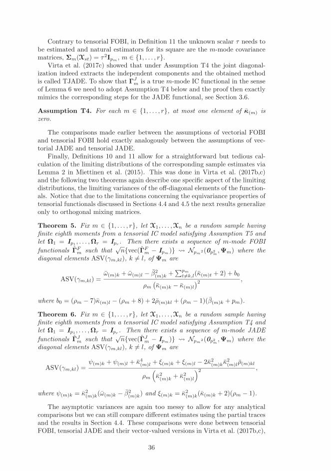
Contrary to tensorial FOBI, in Definition 11 the unknown scalar τ needs tobe estimated and natural estimators for its square are the m-mode covariancematrices, Σm(Xst) = τ2Ipm , m ∈ 1, . . . , r.

Virta et al. (2017c) showed that under Assumption T4 the joint diagonal-ization indeed extracts the independent components and the obtained methodis called TJADE. To show that ΓJm is a true m-mode IC functional in the senseof Lemma 6 we need to adopt Assumption T4 below and the proof then exactlymimics the corresponding steps for the JADE functional, see Section 3.6.

Assumption T4. For each m ∈ 1, . . . , r, at most one element of κ(m) iszero.

The comparisons made earlier between the assumptions of vectorial FOBIand tensorial FOBI hold exactly analogously between the assumptions of vec-torial JADE and tensorial JADE.

Finally, Definitions 10 and 11 allow for a straightforward but tedious cal-culation of the limiting distributions of the corresponding sample estimates viaLemma 2 in Miettinen et al. (2015). This was done in Virta et al. (2017b,c)and the following two theorems again describe one specific aspect of the limitingdistributions, the limiting variances of the off-diagonal elements of the function-als. Notice that due to the limitations concerning the equivariance properties oftensorial functionals discussed in Sections 4.4 and 4.5 the next results generalizeonly to orthogonal mixing matrices.

Theorem 5. Fix m ∈ 1, . . . , r, let X1, . . . ,Xn be a random sample havingfinite eighth moments from a tensorial IC model satisfying Assumption T5 andlet Ω1 = Ip1 , . . . ,Ωr = Ipr . Then there exists a sequence of m-mode FOBI

functionals ΓFm such that√nvec(ΓFm − Ipm) Npm2(0p2m ,Ψm) where the

diagonal elements ASV(γm,kl), k 6= l, of Ψm are

ASV(γm,kl) =ω(m)k + ω(m)l − β2

(m)k +∑pmt6=k,l(κ(m)t + 2) + b0

ρm(κ(m)k − κ(m)l

)2 ,

where b0 = (ρm − 7)κ(m)l − (ρm + 8) + 2ρ(m)kl + (ρm − 1)(β(m)k + pm).

Theorem 6. Fix m ∈ 1, . . . , r, let X1, . . . ,Xn be a random sample havingfinite eighth moments from a tensorial IC model satisfying Assumption T4 andlet Ω1 = Ip1 , . . . ,Ωr = Ipr . Then there exists a sequence of m-mode JADE

functionals ΓJm such that√nvec(ΓJm − Ipm) Npm2(0p2m ,Ψm) where the

diagonal elements ASV(γm,kl), k 6= l, of Ψm are

ASV(γm,kl) =ψ(m)k + ψ(m)l + κ4(m)l + ξ(m)k + ξ(m)l − 2κ2(m)kκ

2(m)lρ(m)kl

ρm

(κ2(m)k + κ2(m)l

)2 ,

where ψ(m)k = κ2(m)k(ω(m)k − β2(m)k) and ξ(m)k = κ2(m)k(κ(m)k + 2)(ρm − 1).

The asymptotic variances are again too messy to allow for any analyticalcomparisons but we can still compare different estimates using the partial tracesand the results in Section 4.4. These comparisons were done between tensorialFOBI, tensorial JADE and their vector-valued versions in Virta et al. (2017b,c),

36

establishing in particular that the tensor methods’ lack of affine equivarianceis negligible when compared to the effects of vectorization. Finally, to validatethe results, plugging in r = 1, ρ1 = 1 and simplifying reverts the asymptoticvariances in Theorems 5 and 6 to those in Theorems 3 and 4.

Remark 1. Virta et al. (2017b,c) defined also a second set of cumulant matri-ces Cij, yielding alternative FOBI and JADE m-mode functionals to the onesin Definitions 10 and 11. However, the former is generally asymptotically infe-rior to ΓFm and the latter is asymptotically equivalent to ΓJm and we have thuswithheld from reviewing them here.

37

5 Independent component analysis forfunctional data

5.1 Hilbert space theory

Our last topic treats the independent component analysis of multivariate func-tional data. While functional data analysis can in a sense be seen as statisticsin an infinite-dimensional Euclidean space, the notations between this and theprevious sections are still anything but compatible. Hence in this section wepresent yet another, final set of notation. See Conway (2013); Hsing and Eubank(2015) for a more comprehensive discussion.

Let T be a closed interval on R and let (H0, 〈·, ·〉0) be a real, separableHilbert space of functions from T to R. The geometry of the space is entirelydetermined by the inner product 〈·, ·〉0, which induces the corresponding norm,

‖f‖0 = 〈f, f〉1/20 , and the metric, d0(f, g) = ‖f − g‖0, for f, g ∈ H0. Theprevious concepts already provide analogies for several central concepts of mul-tivariate statistics but some key ones are still missing, most notably matrices,the generalization of which is given by bounded linear operators. An operatorL : H0 → H0 is said to bounded if the operator norm, ‖L‖OP = infM ≥ 0 |∀f ∈ H0 : ‖Lf‖0 ≤M‖f‖0, is finite, and linear if L(af+g) = aL(f)+L(g), forall a ∈ R, f, g ∈ H0, both familiar properties of matrices. The set of all boundedlinear operators from H0 to H0 is denoted by L(H0) and forms a Banach spacewhen equipped with the operator norm ‖ · ‖OP.

We next introduce analogies of several familiar notions of linear algebrato linear operators. The identity operator id ∈ L(H0) leaves any functionunchanged, id f = f , for all f ∈ H0. Similar to the matrix transpose, everybounded linear operator has the adjoint operator L∗ : H0 → H0 determineduniquely by the relation, 〈Lf, g〉0 = 〈f, L∗g〉0, for all f, g ∈ H0. If an operatorsatisfies L = L∗ it is called self-adjoint and if further 〈Lf, f〉0 ≥ 0, for all f ∈H0, we say that L is positive semidefinite. A self-adjoint, positive semidefiniteoperator L is said to be a trace-class operator if

∑∞k=1〈Lek, ek〉 converges for

some orthonormal basis ek, k ∈ N+, in which case its trace, tr(L), is definedas the previous quantity (which is independent of the choice of the basis ek).If both of the identities, UU∗ = id and U∗U = id, hold for an operator U theoperator is called unitary. Finally, the simplest way of constructing boundedlinear operators is akin to using the vectors a,b to obtain the rank-1 matrixab>: for every pair of functions, g, h ∈ H0, the tensor product operator (g⊗h) :H0 → H0 acting as (g ⊗ h)f = 〈h, f〉0 · g is a bounded linear operator.

To be able to do statistics in H0 we introduce randomness to the space bybriefly returning to the measure-theoretic notions discussed back in Section 2.Recalling our probability space, (Ω,F ,P), a random function is defined to beany mapping X : Ω → H0 which is F/B-measurable where B is the Borel-algebra generated by the open sets in H0 with respect to the induced metric d0.To aid visualization, a random sample of simulated functional data is depicted

38

0.0 0.2 0.4 0.6 0.8 1.0

−1

01

2

t

x(t)

Figure 5.1: A random sample of n = 40 functions from a particular distribution.

in Figure 5.1. Similarly, a random operator is defined as any mapping X : Ω→L(H0) which is F/BOP-measurable where BOP is the Borel-algebra generatedby the open sets in L(H0) with respect to the metric induced by the operatornorm.

The Riesz representation theorem can next be used to define expected val-ues for both random functions and operators. If the random function X isbounded in the sense that E(‖X‖0) < ∞, then there exists a unique func-tion µ ∈ H0 such that E(〈X, f〉0) = 〈µ, f〉0, for all f ∈ H, and we defineE(X) = µ. Analogously, if the random operator W is bounded in the sense thatE(‖W‖OP) < ∞, then there exists a unique bounded linear operator Υ suchthat E(〈Wf, g〉0) = 〈Υf, g〉0, for all f, g ∈ H0 and we again define E(W ) = Υ.

With the tensor product and the expected values at hand, we are nowequipped to quantify variation in functional spaces. Assuming that the ran-dom function X is centered, i.e. E(X) = 0, and has finite second moments,E(‖X‖20) <∞, the covariance operator of X is the self-adjoint, positive semidef-inite, trace class operator Σ(X) = E(X⊗X). Like its multivariate counterpart,also the covariance operator can be shown to admit an eigendecomposition:Σ(X) =

∑∞k=1 λk(φk ⊗ φk) where λk = 〈Σφk, φk〉0, k ∈ N+, are the non-

negative eigenvalues in decreasing order and the eigenvectors φk, k ∈ N+, forman orthonormal basis of H0, that is, 〈φk, φl〉0 = δkl. The concept of functionalprincipal component analysis would now naturally follow but we will postponeits discussion to Section 5.2 where we also review other models for functionaldata.

From this point onwards, we abandon the familiar course of presentationused in the previous two parts of the summary. Infinite-dimensional data fun-damentally differs from the finite-dimensional in various important aspects andthis means that generalizations of some everyday objects from multivariatestatistics to H0 are sometimes very difficult to obtain. For example, inverses ofoperators can be rather ill-behaved in H0 and as a consequence the standard-ization of random variables is not feasible in the usual sense, an issue we discusscloser in Section 5.3. However, we will still review the related methodology andmodels insofar as they exist.

39

5.2 Functional data models

Whereas in finite-dimensional setting the different classes of methods were uni-fied through their connection to the location-scatter and normal models thisno longer holds for functional data and the extensions of the previous modelsare of a more disconnected variety. We assume in the following, without lossof generality, that all random functions X are centered, E(X) = 0, and beginby describing Gaussian random elements in H0, the functional version of thenormal distribution.

A random function X is said to be Gaussian if 〈X, f〉0 is normally dis-tributed for all f ∈ H0 (Lifshits, 2012). As an immediate consequence, anyfinite tuple (〈X, f1〉0, . . . , 〈X, fp〉0) has a multivariate normal distribution bythe Cramer-Wold device. Any Gaussian function X in H0 is square integrable,E(‖X‖2) < ∞, and furthermore the distribution of a zero-mean Gaussian ran-dom function X is uniquely determined by its covariance operator Σ(X). How-ever, contrary to the finite-dimensional Euclidean spaces, not every self-adjoint,positive semidefinite operator L ∈ L(H0) defines a Gaussian distribution. Acounterexample is given by the simplest bounded linear operator, the identityoperator id. A heuristic reason for this is that the sequence of eigenvalues ofany bounded, self-adjoint, positive semidefinite operator must converge to zero,something id with its infinite sequence of unit eigenvalues fails to do. If H0 is areproducing kernel Hilbert space (Paulsen and Raghupathi, 2016), meaning thatpoint evaluation is representable for all t ∈ T as f(t) = 〈f, gt〉, for some gt ∈ H0,any finite collection of time points, X(t1), . . . , X(tm), has a joint Gaussian dis-tribution. The resulting Gaussian functions are in stochastic analysis generallycalled Gaussian processes and some classes of covariance functions commonlyused with Gaussian processes include the set of squared exponential covariancefunctions and the set of Matern covariance functions (Rasmussen and Williams,2006).

A classical method of functional data analysis which behaves particularlywell for Gaussian functions is functional principal component analysis (FPCA),better known under the name of Karhunen-Loeve expansion, see Bosq (2012).Assume that the covariance operator of the random function X has the eigen-decomposition Σ(X) =

∑∞k=1 λk(φk ⊗ φk). As the eigenvectors form an or-

thonormal basis of H0, the identity operator id : H0 → H0 can be written asid =

∑∞k=1(φk⊗φk), and we have the representation X =

∑∞k=1〈φk, X〉0φk. As

in the multivariate case, the “principal components” mk = 〈φk, X〉0 are uncor-related and have the corresponding eigenvalues as their variances, E(mkml) =δklλk. If X is now a Gaussian function, our previous derivations reveal that theprincipal components mk are independent N (0, λk)-distributed random vari-ables and dimension reduction into a finite sub-space of H0 can be carried outby truncating the expansion at a chosen value of k. Numerous extensions ofFPCA and the Karhunen-Loeve expansion have been proposed over the years,see Yao et al. (2005); Ramsay and Silverman (2006); Bali et al. (2011).

As we saw earlier, id is not a feasible covariance operator in H0 and con-sequently pursuing functional elliptical and independent component models viathe generalization of the properties of a “standardized” Gaussian function willnot work. However some tricks can be used to arrive at extensions of familiarmodels, such as the elliptical functional models considered in Bali and Boente(2009); Boente et al. (2014). A random function X is said to have an ellip-

40

tical distribution with parameters µ ∈ H0 and Σ ∈ L(H0), where Σ is self-adjoint, positive semidefinite, compact operator, if for any bounded linear op-erator A : H0 → Rd the random vector AX is elliptically distributed with theparameters Aµ and AΣA∗. Essentially, a random function is elliptical if all itsfinite-dimensional reductions are. The resulting class of elliptical random func-tions shares many of the properties of its finite-dimensional cousin: if the meanand covariance operator of an elliptical function exist they equal respectively µand ρΣ, for some ρ > 0; the conditional expectations of finite-dimensional pro-jections of elliptical functions admit simple expressions and the class of ellipticalfunctions is a superset of the set of Gaussian functions.

In addition to PCA, the recent years have seen a wide range of classical mul-tivariate methods being extended to functional data, including non-parametricmethods (Yao et al., 2005; Ferraty and Vieu, 2006), linear modelling (Ramsayand Silverman, 2006; Horvath and Kokoszka, 2012), canonical correlation (Heet al., 2004; Ramsay and Silverman, 2006; Hsing and Eubank, 2015) and suf-ficient dimension reduction (Ferre and Yao, 2003, 2005; Hsing and Ren, 2009).In practice, the application of all the previous methods to observed data re-quires one intermediate step: as we can never observe anything truly infinite-dimensional, the obtained discrete data points need to be smoothed into func-tions by fitting them into an appropriate, (finite-dimensional) functional basis.Excellent account of smoothing can be found, for example, in Ramsay and Sil-verman (2006) and consequently we will refrain from discussing it here.

Finally, also our main topic has received its functional counterpart. In Liet al. (2015) a functional version of independent component analysis was devel-oped and due to its close connection to the multivarite functional ICA of Virtaet al. (2017a) we will devote the next section to it.

5.3 Functional ICA

A first hurdle in defining independent component analysis in spaces of infinitedimension is given by the concept of independence itself. A random function Xdoes not per se consist of any distinct components we could consider as inde-pendent and the independence must somehow be contained within the functionitself. Along these lines Li et al. (2015) defined a random function X to be in-dependent if its coordinates 〈X,φk〉0, k ∈ N+, with respect to some particularpredefined basis φk, k ∈ N+, ofH0 define a set of independent random variables.An infinite collection of random variables is said to be independent if all of itsfinite subsets consist of mutually independent random variables. The same def-inition for the independence of X is used also by Gutch and Theis (2012) whoin addition require that the orthogonal projection to any subspace spanned by asubset of the basis is independent with the projection to the complement of thesubspace. A key question is then the determination of the basis φk, all followingresults greatly depending on the choice. In a finite Euclidean space a naturalcandidate is the corresponding canonical basis but no such concept exists forgeneral Hilbert spaces. The choice of Li et al. (2015) is to use an eigenbasis ofthe covariance operator of X as this canonical basis and consequently they areable to define the functional IC model.

Definition 12. Let X be a random element in H0 with E(‖X‖20) <∞ and letφk, k ∈ N+, be an eigenbasis of Σ(X). Then we say that X obeys the functional

41

independent component model if there exists an operator Γ ∈ L(H0) such thatΓX has independent components with respect to the basis φk.

As the simplest IC method, FOBI seems again like the most reasonable start-ing point for functional generalization but additional obstacles are encounteredalready at the first step of the procedure, the standardization: a standardizedfunction would need to have the identity operator as its covariance operator,something we already deemed impossible. As the standardization is an integralpart of FOBI and required in the subsequent step, Li et al. (2015) bypass thisbarrier by assuming that the unmixing operator Γ in Definition 12 is of a veryspecific form. Namely, they require that for some fixed d, the operator Γ actsonly on a subspace spanned by the d first basis vectors φk, effectively reduc-ing the separation problem from infinite- to finite-dimensional. If we denoteMd = span(φ1, . . . , φd) and let Pd and Qd be respectively the projections ontothe span and its orthogonal complement, the assumption can be written as

Γ = PdAPd +Qd, (5.1)

for some bounded linear operator A ∈ L(H0). In the following this form ofthe model will be called a d-dimensional functional IC (d-FIC) model and thedimension d is henceforth assumed to be fixed.

One way to motivate the simplification is via Gaussian functions; the mutu-ally independent principal components mk+1,mk+2, . . . in the Karhunen-Loeveexpansion of the simplified model behave as if the original function was Gaus-sian. As normal distribution is a common choice for the distribution of errors inclassical models, the previous allows us to consider the tail of the expansion asnoise and the subspace Md as the “signal subspace”. Similar problems involv-ing standardization in functional spaces have been solved using, for example,regularization (Li and Song, 2017). Let next X(d) = PdX and Z(d) = PdZ bethe projections of the observed and latent function into the signal subspace, towhich we may without loss of generality restrict ourselves.

To solve the functional IC model it is thus sufficient to find any operator Γ ∈L(H0) such that ΓX(d) has independent components. However, we again requiresome additional structure from the estimators, as put forth in the followingdefinition.

Definition 13. The functional Γ : D → L(Md) is a d-dimensional functionalindependent component (d-FIC) functional if, for all X(d) coming from a d-FICmodel, we have,

i) Γ(X(d))X(d) has independent components and

ii) Γ(X(d))X(d) = Γ(AX(d))AX(d) for all invertible linear operators A ∈L(H0)

Definition 13 clearly parallels Definitions 2 and 9 but with one importantdistinction: the invariance property rests entirely on the assumption that thed-FIC model is accurate. In particular, the invariance is unlikely to hold in anypractical situation, a price we have to pay for moving the concepts of ICA tothe infinite-dimensional spaces.

Having solved the main issue caused by the infinite dimensionality of thespace, Li et al. (2015) next defined a functional counterpart for the FOBI-matrix

42

using the tensor product,

B(X) = E (X ⊗X) (X ⊗X) = E‖X‖20 (X ⊗X)

,

and showed that it exists and has an eigendecomposition under the assumptionof finite fourth moments, E(‖X‖4) < ∞. The pair of operators, Σ(X), B(X),now shares many of the properties (equivariance, positive semidefiniteness) oftheir multivariate progenitors, not the least of which is the ability to solve thefunctional IC model. Standardization being now possible, Li et al. (2015) provedthat,

Σ(X(d))−1/2X(d) = UΣ(Z(d))−1/2Z(d) (5.2)

for some unitary operator U ∈ L(H0), showing that also now standardizationsolves the first half of the problem. By Σ(X(d))−1/2 we refer to any inversesquare root of the covariance operator Σ(X(d)) and as we did not make anyidentifiability constraints on Z also Σ(Z(d))−1/2 appears in the formula con-trary to (3.5) and (4.3). We denote the standardized function in the following

by X(d)st = Σ(X(d))−1/2X(d) and it naturally satisfies Σ(X

(d)st ) = Pd, where the

projection operator Pd is equivalent to the identity operator inside Md. Ap-proaching then the second part (“rotation”) via fourth moments as in regularFOBI yields fruitful results and goes to show that the FOBI-methodology seemsto know no limits in its areas of application. We define next the correspondingfunctional IC functional.

Definition 14. Let X come from a d-FIC model with the covariance opera-tor eigenbasis φk, k ∈ N+. Then the functional FOBI-functional is ΓFF =

HΣ(X(d))−1/2 where H =∑dk=1(φk ⊗ ψk) and ψk, k ∈ 1, . . . , d, are the

eigenvectors of the FOBI-operator,

B(X(d)st ) =

d∑

k=1

τk(ψk ⊗ ψk).

Contrary to our earlier IC functionals the current unorthodox relationship ofthe model with the eigenbasis of the covariance operator forces us to define theIC functional in Definition (17) only for data coming from the corresponding ICmodel. The functional FOBI-functional can be shown to be a d-FIC functionalunder the following, familiar-looking assumption.

Assumption F1. The excess kurtoses E(〈Z, φk〉40) − 3, k ∈ 1, . . . , d, aredistinct.

To apply the above methods to extract the independent components from afunctional data sample assumed to obey the d-FIC model, a coordinate repre-sentation of the above was developed in Li et al. (2015), essentially translatingthe whole procedure into the form of linear algebra.

Other excursions into the functional realm from the viewpoint of ICA in-clude: Gutch and Theis (2012) who discuss conditions for the identifabilityof the infinite-dimensional IC model, Rendon et al. (2014) who defined kur-tosis for functional data and used it for clustering and Virta et al. (2017a)who developed a framework for conducting independent component analysis for

43

multivariate functional data. The multivariate functional setting is in a sense amore logical choice for functional ICA than the univariate one as the conceptof independence is in the former naturally defined as a property between thecomponent functions. However, this freedom comes at the price of compromis-ing the identifiability of the corresponding IC model. This and other aspects ofthe multivariate ICA methodology will be the topics of our final section.

5.4 Multivariate functional ICA

Multivariate functional data

Before moving on to the multivariate functional IC model we first describe theconcept of multivariate functional data itself. Let H = H0 × . . . × H0 be ap-variate functional space with identical component spaces H0 as described inSection 5.1. The elements of H are multivariate functions f = (f1, . . . fp) fromthe interval T to Rp. In practice a sample of multivariate functional data looksvery much as the univariate functional sample in Figure 5.1, only that now wehave p such curves for each individual. Now, H is as a direct sum of Hilbertspaces itself a Hilbert space, meaning that everything we wrote in Section 5.1holds for multivariate functional data as well. However, we next introduce viathe choice of inner product and linear operators some additional structure to Hthat ties its properties closely to those of its component spaces.

First, the geometry of the space is inherited from the component spaces bydefining the inner product as 〈f, g〉 =

∑pj=1〈fj , gj〉0, for all f = (f1, . . . , fp),

g = (g1, . . . , gp) ∈ H. The induced norm then satisfies ‖f‖2 =∑pj=1 ‖fj‖20.

Our collection of bounded linear operators is likewise defined via the operatorsof the component spaces: the set L(H) consists of all operators from H to Hwhich act as f 7→ (

∑pj=1 L1jfj , . . . ,

∑pj=1 Lpjfj) for some collection of bounded

linear operators Lij ∈ L(H0) | i, j ∈ 1, . . . , p. The action resembles closelyordinary matrix multiplication and, indeed, if we represent the operator as

L =

L11 · · · L1p

.... . .

...Lp1 · · · Lpp

the mapping f 7→ Lf can be carried out using the rules for matrix multiplica-tion. Basic functional analysis can be used to show that any operator in L(H)is bounded and linear. Two natural subclasses of L(H) stand out: unitary op-erators U which satisfy

∑pk=1 UikUjk = δij · id, for all i, j ∈ 1, . . . , p, and

diagonal operators L for which Lij = 0 for all i 6= j.Despite the current surge of interest in functional data, multivariate func-

tional data has received considerably less attention in the literature. Multi-variate functional PCA has been considered in Ramsay and Silverman (2006);Berrendero et al. (2011); Sato (2013); Chiou et al. (2014); Jacques and Preda(2014); Happ and Greven (2016), multivariate functional clustering in Tokushigeet al. (2007); Kayano et al. (2010); Ieva et al. (2011); Jacques and Preda (2014),multivariate functional sufficient dimension reduction in Li and Song (2017) and,finally, multivariate independent component analysis in Virta et al. (2017a), themethodology of which we review next.

44

Multivariate functional IC model

Call the component functions of X = (X1, . . . , Xp) independent if for all mea-surable mappings g1, . . . , gp : H0 → R the vector (g1(X1), . . . , gp(Xp)) ∈ Rp ofreal-valued random variables has independent components. The multivariatefunctional IC model can then be defined without reference to any basis.

Definition 15. Let X be a random function in H. Then we say that X obeys themultivariate functional independent component model if there exists an operatorΓ ∈ L(H) such that the component functions of ΓX are independent.

The lack of the eigenbasis of the covariance operator in Definition 15 meansthat we also avoid the need for any moment assumptions on X. Yet, suchfreedom is only temporary as again attempting to fit any analogue of standard-ization into the model leads into problems. Before that, however, we discuss amore pressing matter. The independence of the component functions of Z isnaturally preserved under any map Z 7→ DZ where D ∈ L(H) is a diagonaloperator. Thus, we can only hope to estimate the independent components upto transformations by some arbitrary linear operators and the recovering of the“original” components in any form cannot be guaranteed without strong addi-tional assumptions on the model. However, this non-uniqueness sounds moreadverse than it actually is in practice and Virta et al. (2017a) showed thatvarious practical uses and interpretations can still be given to the extractedcomponents.

The same restriction as in Li et al. (2015) was used also in Virta et al. (2017a)to solve issue with the standardization. That is, let the covariance operator ofthe observed multivariate random function X = (X1, . . . , Xp) be the matrix ofoperators,

Σ(X) = E (X ⊗X) =

E (X1 ⊗X1) · · · E (X1 ⊗Xp)...

. . ....

E (Xp ⊗X1) · · · E (Xp ⊗Xp)

.

The same arguments as in the univariate case show that Σ(X) is adjoint, pos-itive semidefinite, trace-class operator and admits a spectral decomposition,∑∞k=1 λk(φk ⊗ φk) where the eigenvalues λk are in a decreasing order. Letting

again Md = span(φ1, . . . , φd) for some fixed d, we assume that Γ in Definition15 is of the form (5.1) for some A ∈ L(Md), where Pd and Qd are again respec-tively the projections onto Md and its orthogonal complement. If a randomfunction X ∈ H obeys such a model for some fixed d, we say that X follows ad-dimensional multivariate functional independent component (d-MFIC) model.

The definition of a solution of the simplified IC model is given next in theform of a functional, where once again we have been obliged to modify ourexpectations of an IC functional to best suit the particular model and form ofthe data.

Definition 16. The functional Γ : D → L(Md) is a d-dimensional multivariatefunctional independent component (d-MFIC) functional if, for all X(d) comingfrom a d-FIC model, we have,

i) Γ(X(d))X(d) can be divided into subvectors of functions so that each sub-vector corresponds to exactly one of the components of Z and is indepen-dent with the remaining p− 1.

45

The change in the first condition over the univariate functional IC functionalin Definition 13 is caused by the interplay of the two conflicting forms of “di-mensionality”, p and d. Namely, if d < p then we clearly cannot estimate all pcomponent functions and if d > p some of the estimated components must nec-essarily correspond to the same component of Z. Based on this a rule of thumbd = p was advocated in Virta et al. (2017a). Furthermore, we have completelydispensed with any invariance or equivariance of the functionals as the secondof our two primary estimators for the model does not admit such properties.However, this is only an aesthetic setback as the property ii) was in Definition13 in any case completely theoretical and said nothing about the application ofthe methodology to real data.

Finally, it is not too much of a surprise to see that after the restriction to thefinite-dimensional model, standardization by Σ(X(d)) leaves us a unitary trans-formation away from our objective. Namely, if we again denote by Σ(X(d))−1/2

an inverse square root of Σ(X(d)), we have,

Σ(X(d))−1/2X(d) = UΣ(Z(d))−1/2Z(d),

for some unitary U ∈ L(H). The estimation of the missing U is then our finaltask, something Virta et al. (2017a) achieved by generalizing both FOBI andJADE to multivariate functional data.

Multivariate functional FOBI and JADE

For our final extensions of FOBI and JADE we still require another set of“cumulant matrices”, this time in the form of linear operators in Md. In somesense the canonical basis of the space is ψ1, . . . , φd and mimicking the formulafor (3.7) prompts us to define,

Cij(X) = E 〈X,φi〉〈X,φj〉 (X ⊗X) − E 〈X,φi〉〈X∗, φj〉 (X ⊗X∗) (5.3)

− E 〈X,φi〉〈X∗, φj〉 (X∗ ⊗X) − E 〈X,φi〉〈X,φj〉 (X∗ ⊗X∗) ,

where X∗ is an independent copy of X and the assumption of finite fourth mo-ments, E(‖X‖4) <∞, is sufficient for the existence of the operators. Again theextensions have no other motivation than analogy and once more that turns tobe enough. Our interest lies with standardized random functions X, satisfyingΣ(X) = Pd, and for any such function simplifying (5.3) reveals the familiarform,

Cij(X) = E 〈X,φi〉〈X,φj〉 (X ⊗X) − φi ⊗ φj − φj ⊗ φi − δij · Pd.

Further substituting X = UZ, where U is unitary and Z = (Z1, . . . , Zp) hasindependent component functions, to the previous yields Cij(UZ) = UDijU∗

for some diagonal operator Dij = Dij(UZ), the exact form of which is given inVirta et al. (2017a). This implies that the missing unitary operator once again“diagonalizes” all operators Cij(Xst), soon leading us to yet another forms ofFOBI and JADE. However, one needs to remember that we are currently playingwith two clashing forms of diagonality, the algebraic diagonality in the sense ofspectral decompositions and the physical diagonality in the sense of diagonaloperators. The operators Dij belong to the latter group and to be able to usespectral decompositions of the cumulant operators to extract U Virta et al.

46

(2017a) introduced a connection between the two identically named concepts.To avoid overt repetition we refrain from paraphrasing their results here andsimply state later the assumptions which are required for the connections tohold. Note that for Euclidean spaces these problems are averted as the twoforms of diagonality exactly coincide.

The corresponding multivariate functional FOBI-operator for a standardizedfunction X also has a recognizable structure,

C(X) = E (X ⊗X) (X ⊗X) − (d+ 2) · Pd,

and is easily shown to satisfy C(UX) = UC(X)U∗ for any unitary U andstandardized X. Based on our earlier discussion C(Z) is a diagonal operatorand the spectral decomposition of the FOBI-operator proves sufficient groundsfor defining the next IC functional.

Definition 17. Let X come from a d-MFIC model with the covariance operatoreigenbasis φk, k ∈ N+. Then the multivariate functional FOBI-functional isΓMFF = HΣ(X(d))−1/2 where H is the linear operator with the action,

f 7→ (E1(ψ1 ⊗ ψ1)f, . . . , E1(ψd ⊗ ψd)f) ,

for all f = (f1, . . . fp) ∈Md where E1 :Md → H0 is a linear operator (projec-tion) that “picks” the first component of a multivariate function, E1f = f1 and

ψk, k ∈ 1, . . . , d, are the eigenvectors of the FOBI-operator C(X(d)st ).

The multivariate functional FOBI-functional was shown to be a d-MFICfunctional in Virta et al. (2017a) under Assumption M1 below. Additionally, itcould be shown to be affine equivariant under the d-MFIC-model using analo-gous arguments to Li et al. (2015).

Assumption M1. The eigenvalues of C(Z(d)st ) are distinct.

Sadly, no simple interpretations for the assumption through, e.g, “functionalkurtosis” can be given.

The peculiar form of the FOBI functional stems from the identifiabilityproblems discussed after the introduction of the model in Definition 12. Ev-

ery projection (ψk ⊗ ψk)X(d)st , k ∈ 1, . . . , d, onto an eigenvector defines a

full p-variate random function in a 1-dimensional space where the only depen-dence on the independent components is through the inner products 〈ψk, Xst〉,k ∈ 1, . . . , d, each of which corresponds to exactly one latent function Xj .Thus the actual functional forms of the projections tell us nothing about theindependent components and Virta et al. (2017a) actually equated the solutionof the model with this d-vector of inner products. For the same reason thechoice of the projection E1 in Definition 15 is completely arbitrary and anyother coordinate projection, E2, . . . , Ep, could have been used as well.

Moving on to our extension of JADE, one thing we are still missing is a wayto combine the information in the cumulant operators Cij . We thus need aconcept of joint diagonalizer (understood in the spectral sense) for self-adjointlinear operators. Mimicking the standard finite-dimensional definition (3.9)Virta et al. (2017a) defined the joint diagonalizer of the set of operators in

47

Md, S = Sj ∈ L(Md) | j ∈ 1, . . . ,m to be the orthonormal basis ψk,k ∈ 1, . . . , d, of Md that maximizes the objective function,

w(ψ1, . . . , ψd) =

m∑

j=1

d∑

k=1

〈Sjψk, ψk〉2. (5.4)

With that, the definition of the JADE functional now easily follows.

Definition 18. Let X come from a d-MFIC model with the covariance opera-tor eigenbasis φk, k ∈ N+. Then the multivariate functional JADE-functionalis ΓMFJ = HΣ(X(d))−1/2 where H and E1 are as in Definition 17 but thefunctions ψk, k ∈ 1, . . . , d, now constitute the joint diagonalizer of the set

C = Cij(X(d)st ) | i, j ∈ 1, . . . , d.

To show the Fisher consistency of ΓMFJ , we again need some connectionbetween the spectral diagonalization offered by the joint diagonalization in (5.4)and the physical diagonality of the operators Dij , and, indeed, under two tech-nical conditions (Virta et al., 2017a) this is achieved and the multivariate func-tional JADE-functional is a d-MFIC functional.

After having extracted the independent components in the form of the innerproducts using either FOBI or JADE one issue still remains: how to deter-mine which inner products correspond to the same independent component. Inpractice this has little bearing as the value of the components is most likelyassessed by their usefulness in subsequent analyses. However, if some groupingis desired, similar devices to those used in Nordhausen and Oja (2011) in thecontext of independent subspace analysis (ISA) (Cardoso, 1998) could proveuseful in our case as well. ISA can be seen as ICA for block vectors and assuch is actually a finite-dimensional analogue for our current problem. Againcoordinate representation of the methods can be devised, using which smoothedobserved functional data can be subjected to the two methods.

Finally, our proven form of presentation naturally begs for asymptotical re-sults for the functional IC methods too, but due to the current nonexistence ofsuch results and the general difficulty of moving limiting results from multivari-ate to functional data we choose to stop here.

48

6 Discussion

We end with a short section collecting various directions for future research. Asboth tensorial and functional ICA are still emerging fields much work remainsto be done. The presented extensions of FOBI and JADE serve well as pre-liminary excursions to the topic but if any of the intuition from vector-valuedICA carries over, better estimators are to be expected. Especially linear ICAmethods are likely to have natural extensions in both cases, see for example thevarious forms of group ICA (Calhoun et al., 2009) which, while already targetedto tensor-valued data, rely typically on vectorization. Of special interest is alsothe extension of projection pursuit to the two discussed forms of non-standarddata, especially in the light of Theorem 4 showing that SPP reaches the lim-iting efficiency of JADE with a lighter computational load. Some preliminarycalculations already show that the same relationship holds with TJADE andtensorial PP when we define the latter as search for directions u maximizingthe “tensorial kurtosis”, E(u>X(m)X

>(m)u)2. Replacing then the square with

any smooth enough function g would give us a general-purpose “tensorial Fas-tICA”. Similarly, projection pursuit in the case of univariate functional data isvery straightforwardly postulated and will most likely lead into applying stan-dard FastICA to the vector of functional principal component coefficients.

A major shortcoming of all the presented methods and the key issue pre-venting their large-scale application in practice is the lack of tools for dimensionestimation. To reliably reduce the dimension of tensorial or functional obser-vations a systematic procedure for determining the “correct” dimensionality ofthe latent tensors and functions is called for and the asymptotic and bootstrap-ping schemes developed in Nordhausen et al. (2016, 2017a) for vector-valueddimension reduction will likely provide a valuable starting point for hypothesistesting in the former case, assuming normally distributed noise. Similarly thegeneral order determination technique of Luo and Li (2016) allowing the esti-mation of the rank of any scatter matrix estimate could be used for the samepurpose. Assuming still Gaussian noise, for univariate functional ICA testingfor the dimension is equivalent to testing whether the “tail” of the observedfunction is a Gaussian process. A naıve example test is obtained by choosingmultiple subsets of the tail coordinates with different cardinality and conductinga multivariate test of normality for each.

Third interesting prospect is the studying of the connection between thestatistical tensor methods’ and the traditional tensor decompositions discussedin Section 4.2. Practically any tensor decomposition can be used to define a di-mension reduction method by leaving the mode corresponding to the identicallyand independently distributed sample uncompressed and if the resulting meth-ods are subjected to careful scrutiny, many interesting connections to statisticalmethodology are bound to be revealed.

49

Appendix

Proof of Lemma 1. Without loss of generality we assume that all consideredroots of positive-definite matrices are selected to be the unique positive-definitechoice. Assume first that the conditions of Definition 2 hold for Γ. Then forany z ∈ Rp with independent components we have, V(zst) = Γ(z)Σ(z)1/2 ≡ΓΣ(z)−1/2zΣ(z)−1/2Σ(z)1/2 ≡ Ip, where the first equivalence uses condi-tion ii) of Definition 2 and the second equivalence condition i). Similarly, forarbitrary x ∈ Rp and U ∈ Up×p we have,

V(Uxst) = VUΣ(x)−1/2U>Ux = VΣ(Ux)−1/2Ux = V(Ux)st.

Consequently, by the form of the functional, VUxst = Γ(Ux)Σ(Ux)1/2 ≡Γ(x)U>UΣ(x)1/2U> ≡ Γ(x)Σ(x)1/2U> ≡ V(xst)U

>, where the first equiva-lence uses condition ii) of Definition 2.

Assume then that the two conditions of Lemma 1 hold. Then for any stan-dardized z ∈ Rp with independent components, Γ(z) = V(zst)Σ(z)−1/2 =V(zst) ≡ Ip where the second equality holds as Σ(z) = I and the equivalenceuses condition i) of Lemma 1. Finally, for arbitrary x ∈ Rp and A ∈ Rp×p wehave, Γ(Ax) = V((Ax)st)Σ(Ax)−1/2. By Ilmonen et al. (2012) Σ(Ax)−1/2 =WΣ(x)−1/2A−1, where the orthogonal matrix W ∈ Up×p is chosen so that theinverse root is symmetric. This in turn implies that (Ax)st = Wxst and wehave Γ(Ax) = V(Wxst)WΣ(x)−1/2A−1 ≡ Γ(x)A−1 where the equivalencefollows from the condition ii) of Lemma 1.

Proof of Lemma 4. Starting from the left-hand side of the claim we have,

cm(v>k z

)2=

p∑

l=1

vmklcm(zl)

2

≤p∑

l=1

v2(m−1)kl c2m(zl),

where vkl is the lth element of vk, the equality uses properties 2 and 3 fromLemma 3 and the inequality uses Cauchy-Schwarz to the partition vmklcm(zl) =vklvm−1kl cm(zl). By our assumptions vkl = 0, for 1 ≤ l ≤ k − 1, andcm(zl)

2 ≤ cm(zk)2, for k ≤ l ≤ p. Using these, we get

cm(v>k z

)2 ≤p∑

l=k

v2(m−1)kl c2m(zl) ≤ c2m(zk)

p∑

l=k

v2(m−1)kl ≤ c2m(zk)

p∑

l=k

v2kl ≤ c2m(zk),

where the second-to-last inequality uses the bound, v2(m−1)kl = v2klv

2(m−2)kl ≤ v2kl

and the last inequality the unit length of vk.Now, plugging in vk = ±el for some l ∈ k, . . . , p with cm (zl)2 =

cm (zk)2 instantly reveals that equality holds. The converse is seen to betrue by checking what is implied if the second-to-last inequality above actually

preserves equality. In that case we must have c2m(zk)∑pl=k v

2kl(1−v

2(m−2)kl ) = 0,

all terms and factors of which are non-negative. Thus either c2m(zk) = 0 or, for

50

all l ∈ k, . . . , p, vkl ∈ −1, 0, 1. As k ≤ p we cannot have c2m(zk) = 0 andthus by the unit length constraint vk = ±el for some l ∈ k, . . . , p. Assumethen that the whole chain of inequalities preserves equality. Then both theprevious must hold and the second inequality in the chain must preserve equal-ity. This implies that c2m(zl) = c2m(zk) for the same l ∈ k, . . . , p for whichvk = ±el holds, showing that the postulated condition is not just sufficient butalso necessary for the equality.

Proof of Lemma 5. As in the proof of Lemma 4 we have,

p∑

k=1

cm(v>k z

)2=

p∑

k=1

p∑

l=1

vmklcm(zl)

2

≤p∑

k=1

p∑

l=1

v2(m−1)kl c2m(zl).

Using again the upper bound, v2(m−1)kl ≤ v2kl, now gives the desired inequality.

Straightforward substitution V> = PJ, where P ∈ Pp and J ∈ J p arearbitrary, next reveals that the equality is preserved in this case. To show the

converse we observe exactly when the application of the bound v2(m−1)kl ≤ v2kl

preserves equality: for all k we must have∑pl=1 v

2(m−1)kl c2m(zl) =

∑pl=1 v

2klc

2m(zl)

which is equivalent to requiring∑pl=1 v

2klc

2m(zl)(1− v2(m−2)kl ). All factors in the

terms of the previous sum are non-negative and thus if equality is reachedthen we have for all pairs (k, l) either c2m(zl) = 0 or vkl ∈ −1, 0, 1. By ourassumption at most one of the cumulants is zero so at least p − 1 columns ofV> consist entirely of the elements −1, 0, 1. As V> is orthogonal each of thesecolumns must then contain exactly one ±1 and rest of the entries must be zero,meaning that to achieve orthogonality also the final column must be of the sameform. Thus V> = PJ and we have shown this to be both a sufficient and anecessary condition for equality.

Proof of Lemma 6. The proof is similar to that of Lemma 1. Assume first thatthe conditions of Definition 9 hold. Then, for any X coming from the tensorialIC model with diagonal mixing Dm, m ∈ 1, . . . , r, we have,

Vm(Xst) = Γm(X)Σm(X)1/2∗≡ D−1m (τmD2

m)1/2∗≡ Ipm ≡ Ipm ,

where the first equivalence uses condition i) from Definition 9 and a resultfrom Virta et al. (2017b) that under arbitrary mixing Σm(X) ∝ ΩmΩ>m. Thefinal equivalence ≡ must hold because both Vm(Xst) and Ipm are orthogonalmatrices and thus have fixed scale. Assuming then an arbitrary tensor X andorthogonal matrices U1, . . . ,Ur, we have,

Vm(Xst ×rm=1 Um) = VmX×rm=1 (UmΣm(X)−1/2U>mUm)= Vm[X×rm=1 Σm(X×rm=1 Um)−1/2Um]= Vm(X×rm=1 Um)st

51

where we have used the same trick as in the proof of Lemma 1 along with theorthogonal equivariance of Σm. Consequently,

Vm(Xst ×rm=1 Um) = Γm(X×rm=1 Um)Σm(X×rm=1 Um)1/2

≡ Γm(X)U>mUmΣm(X)1/2U>m

≡ Vm(Xst)U>m,

where the first equivalence uses condition ii) from Definition 9.Assume then that Γm satisfies the conditions of Lemma 6. Now, for any X

coming from the tensorial IC model,

Γm(X) = Vm(Xst)Σm(X)−1/2 = Vm(τZ×rm=1 UmV>m)τmUmD−1m U>m,

where τ, τm ∈ R and we have used the singular value decomposition Ωm =UmDmV>m along with Lemma 2 and Theorem 2 from Virta et al. (2017b). Thesame theorem also shows that τZ = (Z ×rm=1 Dm)st and using conditions ii)and i) of Lemma 6 we get,

Γm(X) ≡ τmVm(Z×rm=1 Dm)stVmU>mUmD−1m U>m∗≡ IpmVmD−1m U>m∗≡ Ω−1m .

Let next the tensor X and the orthogonal U1, . . . ,Ur be arbitrary. Then, as inthe proof of the second condition of Lemma 6 above,

Γm(X×rm=1 Um) = Vm(X×rm=1 Um)stΣm(X×rm=1 Um)−1/2

= Vm(Xst ×rm=1 Um)UmΣm(X)−1/2U>m

≡ Γm(X)U>m,

where the equivalence uses condition ii) of Lemma 6.

52

Summaries of original publications

I ICA is well-known for its limitation concerning the number of Gaussianvariables. In Virta et al. (2016b) this constraint is relaxed and the statisticalproperties of two types of projection pursuit estimators are derived underthe obtained non-Gaussian ICA model. The efficiency of the estimators canbe divided into two parts: how well they separate the signal from the noiseand how well they separate the individual signals from each other. The twoestimators are shown to be asymptotically equivalent with respect to theformer and simulations are used to investigate their differences with respectto the latter. A sequential hypothesis test for estimating the dimension ofthe signal subspace is also proposed.

II Virta et al. (2017b) present the novel concept of tensorial independent com-ponent analysis, a dimension reduction framework for higher-order data.An estimator based on the classical fourth-order method FOBI is proposedand its consistency and limiting distribution are derived under the tenso-rial independent component model. Simulations and a real data examplereveal that for both finite samples and in the limit the proposed estimatoris superior to the commonly used alternative of vectorization.

III An improvement over FOBI in standard independent component analysisis given by JADE which better utilizes the fourth-order information inthe estimation. Motivated by this, Virta et al. (2017c) present tensorialJADE and derive its statistical properties under the tensorial independentcomponent model. Comparisons with both the tensorial FOBI and vectorialICA methods show that the previously mentioned relationship betweenFOBI and JADE continues to hold also for tensorial random variables.

IV A popular example of higher order data is given by fMRI-measurementsand in article Virta et al. (2016c) the methods developed in Virta et al.(2017b,c) are put to use in the context of simulated noisy fMRI-data. Theresults imply that the tensorial ICA model can be used to approximate thestructure of brain image data and that the methods of tensorial ICA canreliably extract signals from noisy, high-dimensional tensor-valued data.

V The growing popularity of functional data has also increased the need forfunctional dimension reduction methodology. In Virta et al. (2017a) anindependent component analysis framework is developed for multivariatefunctional data. The methodology is again based on the ideas behind FOBIand JADE and the obtained two estimators are shown to be Fisher consis-tent under the introduced multivariate functional independent componentmodel. Both simulations and a real data example reveal that the proposedestimators surpass functional principal component analysis in efficiency.

53

References

S.-I. Amari, A. Cichocki, and H. H. Yang. A new learning algorithm for blindsignal separation. In Advances in Neural Information Processing Systems,pages 757–763, 1996.

T. W. Anderson. Nonnormal multivariate distributions: Inference based onelliptically contoured distributions. Technical report, Stanford University,Department of Statistics, 1992.

M. Arashi. Some theoretical results on tensor elliptical distribution. arXivpreprint arXiv:1709.00801, 2017.

J. L. Bali and G. Boente. Principal points and elliptical distributions from themultivariate setting to the functional case. Statistics & Probability Letters,79:1858–1865, 2009.

J. L. Bali, G. Boente, D. E. Tyler, and J.-L. Wang. Robust functional principalcomponents: A projection-pursuit approach. The Annals of Statistics, 39:2852–2882, 2011.

A. Belouchrani, K. Abed-Meraim, J.-F. Cardoso, and E. Moulines. A blindsource separation technique using second-order statistics. IEEE Transactionson Signal Processing, 45:434–444, 1997.

J. R. Berrendero, A. Justel, and M. Svarc. Principal components for multivariatefunctional data. Computational Statistics & Data Analysis, 55:2619–2634,2011.

P. Billingsley. Probability and measure. John Wiley & Sons, 2008.

G. Blanchard, M. Sugiyama, M. Kawanabe, V. Spokoiny, and K.-R. Muller.Non-Gaussian component analysis: A semi-parametric framework for lineardimension reduction. In Advances in Neural Information Processing Systems,pages 131–138, 2005.

G. Boente, M. S. Barrera, and D. E. Tyler. A characterization of elliptical distri-butions and some optimality properties of principal components for functionaldata. Journal of Multivariate Analysis, 131:254–264, 2014.

S. Bonhomme and J.-M. Robin. Consistent noisy independent component anal-ysis. Journal of Econometrics, 149:12–25, 2009.

D. Bosq. Linear processes in function spaces: theory and applications, volume149. Springer Science & Business Media, 2012.

V. Calhoun, T. Adali, L. K. Hansen, J. Larsen, and J. Pekar. ICA of functionalMRI data: An overview. In Proceedings of the 4th International Symposiumon Independent Component Analysis and Blind Signal Separation (ICA2003),pages 281–288, 2003.

54

V. D. Calhoun and T. Adali. Unmixing fMRI with independent componentanalysis. IEEE Engineering in Medicine and Biology Magazine, 25:79–90,2006.

V. D. Calhoun, J. Liu, and T. Adali. A review of group ICA for fMRI data andICA for joint inference of imaging, genetic, and ERP data. Neuroimage, 45:S163–S172, 2009.

J.-F. Cardoso. Source separation using higher order moments. In Proceedingsof the 1989 IEEE International Conference on Acoustics, Speech and SignalProcessing, pages 2109–2112. IEEE, 1989.

J.-F. Cardoso. Multidimensional independent component analysis. In Proceed-ings of the 1998 IEEE International Conference on Acoustics, Speech andSignal Processing, volume 4, pages 1941–1944. IEEE, 1998.

J.-F. Cardoso and A. Souloumiac. Blind beamforming for non-Gaussian signals.In IEE proceedings F (radar and signal processing), volume 140, pages 362–370. IET, 1993.

F. J. Caro-Lopera, G. G. Farıas, and N. Balakrishnan. Matrix-variate distri-bution theory under elliptical models-4: Joint distribution of latent rootsof covariance matrix and the largest and smallest latent roots. Journal ofMultivariate Analysis, 145:224–235, 2016.

A. Chen and P. J. Bickel. Efficient independent component analysis. The Annalsof Statistics, 34:2825–2855, 2006.

J.-M. Chiou, Y.-T. Chen, and Y.-F. Yang. Multivariate functional principalcomponent analysis: A normalization approach. Statistica Sinica, 2014:1571–1596, 2014.

A. Cichocki, R. Zdunek, A. H. Phan, and S.-I. Amari. Nonnegative matrix andtensor factorizations: applications to exploratory multi-way data analysis andblind source separation. John Wiley & Sons, 2009.

A. Cichocki, D. Mandic, L. De Lathauwer, G. Zhou, Q. Zhao, C. Caiafa, andH. A. Phan. Tensor decompositions for signal processing applications: Fromtwo-way to multiway component analysis. IEEE Signal Processing Magazine,32:145–163, 2015.

D. B. Clarkson. A least squares version of algorithm AS 211: The FG diagonal-ization algorithm. Journal of the Royal Statistical Society. Series C (AppliedStatistics), 37:317–321, 1988.

P. Comon. Independent component analysis, a new concept? Signal Processing,36:287–314, 1994.

P. Comon, Y. Qi, and K. Usevich. A polynomial formulation for joint decom-position of symmetric tensors of different orders. In International Conferenceon Latent Variable Analysis and Signal Separation, pages 22–30. Springer,2015.

J. B. Conway. A course in functional analysis, volume 96. Springer Science &Business Media, 2013.

55

L. De Lathauwer, B. De Moor, and J. Vandewalle. A multilinear singular valuedecomposition. SIAM journal on Matrix Analysis and Applications, 21:1253–1278, 2000.

S. Ding and R. D. Cook. Dimension folding PCA and PFC for matrix-valuedpredictors. Statistica Sinica, 24:463–492, 2014.

S. Ding and R. D. Cook. Higher-order sliced inverse regressions. Wiley Inter-disciplinary Reviews: Computational Statistics, 7:249–257, 2015a.

S. Ding and R. D. Cook. Tensor sliced inverse regression. Journal of MultivariateAnalysis, 133:216–231, 2015b.

S. C. Douglas. Fixed-point algorithms for the blind separation of arbitrarycomplex-valued non-Gaussian signal mixtures. EURASIP Journal on Ad-vances in Signal Processing, 2007:036525, 2007.

L. Dumbgen, M. Pauly, and T. Schweizer. M-functionals of multivariate scatter.Statistics Surveys, 9:32–105, 2015.

K.-T. Fang, S. Kotz, and K. W. Ng. Symmetric multivariate and related distri-butions. Chapman and Hall, 1990.

F. Ferraty and P. Vieu. Nonparametric functional data analysis: Theory andpractice. Springer Science & Business Media, 2006.

L. Ferre and A.-F. Yao. Functional sliced inverse regression analysis. Statistics,37:475–488, 2003.

L. Ferre and A.-F. Yao. Smoothed functional inverse regression. StatisticaSinica, 15:665–683, 2005.

J. H. Friedman and J. W. Tukey. A projection pursuit algorithm for exploratorydata analysis. IEEE Transactions on Computers, 100:881–890, 1974.

S. Ghurye and I. Olkin. A characterization of the multivariate normal distribu-tion. The Annals of Mathematical Statistics, 33:533–541, 1962.

A. Gupta and T. Varga. Normal mixture representations of matrix variate el-liptically contoured distributions. Sankhya: The Indian Journal of Statistics,Series A, 57:68–78, 1995.

A. K. Gupta and D. K. Nagar. Matrix variate distributions. CRC Press, 1999.

H. W. Gutch and F. J. Theis. To infinity and beyond: On ICA over Hilbertspaces. In Latent Variable Analysis and Signal Separation, pages 180–187.Springer, 2012.

M. Hallin and C. Mehta. R-estimation for asymmetric independent componentanalysis. Journal of the American Statistical Association, 110:218–232, 2015.

C. Happ and S. Greven. Multivariate functional principal component analysisfor data observed on different (dimensional) domains. Journal of the Ameri-can Statistical Association, 2016. Accepted.

56

T. Hastie and R. Tibshirani. Independent components analysis through productdensity estimation. In Advances in Neural Information Processing Systems,pages 665–672, 2003.

G. He, H.-G. Muller, and J.-L. Wang. Methods of canonical analysis for func-tional data. Journal of Statistical Planning and Inference, 122:141–159, 2004.

L. Horvath and P. Kokoszka. Inference for functional data with applications.Springer Science & Business Media, 2012.

H. Hotelling. Analysis of a complex of statistical variables into principal com-ponents. Journal of Educational Psychology, 24:417, 1933.

T. Hsing and R. Eubank. Theoretical foundations of functional data analysis,with an introduction to linear operators. John Wiley & Sons, 2015.

T. Hsing and H. Ren. An RKHS formulation of the inverse regression dimension-reduction problem. The Annals of Statistics, 37:726–755, 2009.

P. J. Huber. Projection pursuit. The Annals of Statistics, 13:435–475, 1985.

H. Hung and C.-C. Wang. Matrix variate logistic regression model with appli-cation to EEG data. Biostatistics, 14:189–202, 2012.

A. Hyvarinen. Fast and robust fixed-point algorithms for independent compo-nent analysis. IEEE Transactions on Neural Networks, 10:626–634, 1999.

A. Hyvarinen and U. Koster. FastISA: A fast fixed-point algorithm for inde-pendent subspace analysis. In EsANN, pages 371–376, 2006.

F. Ieva, A. M. Paganoni, D. Pigoli, and V. Vitelli. ECG signal reconstruction,landmark registration and functional classification. In 7th Conference onStatistical Computation and Complex System, 2011.

K. Illner, J. Miettinen, C. Fuchs, S. Taskinen, K. Nordhausen, H. Oja, andF. J. Theis. Model selection using limiting distributions of second-order blindsource separation algorithms. Signal Processing, 113:95–103, 2015.

P. Ilmonen and D. Paindaveine. Semiparametrically efficient inference based onsigned ranks in symmetric independent component models. The Annals ofStatistics, 39:2448–2476, 2011.

P. Ilmonen, J. Nevalainen, and H. Oja. Characteristics of multivariate distri-butions and the invariant coordinate system. Statistics & Probability Letters,80:1844–1853, 2010a.

P. Ilmonen, K. Nordhausen, H. Oja, and E. Ollila. A new performance indexfor ICA: Properties, computation and asymptotic analysis. Latent VariableAnalysis and Signal Separation, pages 229–236, 2010b.

P. Ilmonen, H. Oja, and R. Serfling. On invariant coordinate system (ICS)functionals. International Statistical Review, 80:93–110, 2012.

J. Jacques and C. Preda. Model-based clustering for multivariate functionaldata. Computational Statistics & Data Analysis, 71:92–106, 2014.

57

I. Jolliffe. Principal component analysis. Springer Verlag, 2002.

T. Kariya and B. K. Sinha. Robustness of statistical tests. Academic Press,2014.

J. Karvanen and V. Koivunen. Blind separation methods based on Pearsonsystem and its extensions. Signal Processing, 82:663–673, 2002.

J. Karvanen, J. Eriksson, and V. Koivunen. Adaptive score functions for max-imum likelihood ICA. Journal of VLSI signal processing systems for signal,image and video technology, 32:83–92, 2002.

M. Kawanabe. Linear dimension reduction based on the fourth-order cumulanttensor. In International Conference on Artificial Neural Networks, pages 151–156. Springer, 2005.

M. Kayano, K. Dozono, and S. Konishi. Functional cluster analysis via orthonor-malized Gaussian basis expansions and its application. Journal of Classifica-tion, 27:211–230, 2010.

T. G. Kolda and B. W. Bader. Tensor decompositions and applications. SIAMReview, 51:455–500, 2009.

Z. Koldovsky, P. Tichavsky, and E. Oja. Efficient variant of algorithm FastICAfor independent component analysis attaining the Cramer-Rao lower bound.IEEE Transactions on Neural Networks, 17:1265–1277, 2006.

T. Kollo. Multivariate skewness and kurtosis measures with an application inICA. Journal of Multivariate Analysis, 99:2328–2338, 2008.

T. Kollo and D. von Rosen. Advanced multivariate statistics with matrices.Springer Science & Business Media, 2006.

B. Li and J. Song. Nonlinear sufficient dimension reduction for functional data.The Annals of Statistics, 45:1059–1095, 2017.

B. Li, M. K. Kim, and N. Altman. On dimension folding of matrix-or array-valued statistical objects. The Annals of Statistics, 38:1094–1121, 2010.

B. Li, G. Van Bever, H. Oja, R. Sabolova, and F. Critchley. Functional indepen-dent component analysis: an extension of the fourth-order blind identification.2015. Submitted.

L. Li and X. Zhang. Parsimonious tensor response regression. Journal of theAmerican Statistical Association, pages 1–16, 2017.

M. Lifshits. Lectures on Gaussian processes. Springer, 2012.

W. Luo and B. Li. Combining eigenvalues and variation of eigenvectors fororder determination. Biometrika, 103:875–887, 2016.

A. M. Manceur and P. Dutilleul. Maximum likelihood estimation for the tensornormal distribution: Algorithm, minimum sample size, and empirical biasand dispersion. Journal of Computational and Applied Mathematics, 239:37–49, 2013.

58

J. I. Marden. Some robust estimates of principal components. Statistics &Probability Letters, 43:349–359, 1999.

R. A. Maronna and V. J. Yohai. Robust estimation of multivariate location andscatter. Wiley StatsRef: Statistics Reference Online, 1976.

M. Matilainen, K. Nordhausen, and H. Oja. New independent component anal-ysis tools for time series. Statistics & Probability Letters, 105:80–87, 2015.

D. S. Matteson and R. S. Tsay. Independent component analysis via distancecovariance. Journal of the American Statistical Association, pages 1–16, 2017.

P. McCullagh. Tensor methods in statistics. Chapman and Hall London, 1987.

J. Miettinen, K. Nordhausen, H. Oja, and S. Taskinen. Fast equivariant JADE.In Proceedings of the 2013 IEEE International Conference on Acoustics,Speech and Signal Processing, pages 6153–6157. IEEE, 2013.

J. Miettinen, K. Nordhausen, H. Oja, and S. Taskinen. Deflation-based Fas-tICA with adaptive choices of nonlinearities. IEEE Transactions on SignalProcessing, 62:5716–5724, 2014a.

J. Miettinen, K. Nordhausen, H. Oja, and S. Taskinen. Deflation-based separa-tion of uncorrelated stationary time series. Journal of Multivariate Analysis,123:214–227, 2014b.

J. Miettinen, S. Taskinen, K. Nordhausen, and H. Oja. Fourth moments andindependent component analysis. Statistical Science, 30:372–390, 2015.

J. Miettinen, K. Nordhausen, H. Oja, S. Taskinen, and J. Virta. The squaredsymmetric FastICA estimator. Signal Processing, 131:402–411, 2017.

E. Moreau. A generalization of joint-diagonalization criteria for source separa-tion. IEEE Transactions on Signal Processing, 49:530–541, 2001.

K. Nordhausen and H. Oja. Independent subspace analysis using three scattermatrices. Austrian Journal of Statistics, 40:93–101, 2011.

K. Nordhausen and D. E. Tyler. A cautionary note on robust covariance plug-inmethods. Biometrika, 102:573–588, 2015.

K. Nordhausen, H. Oja, and E. Ollila. Robust independent component analysisbased on two scatter matrices. Austrian Journal of Statistics, 37:91–100,2008.

K. Nordhausen, P. Ilmonen, A. Mandal, H. Oja, and E. Ollila. Deflation-basedFastICA reloaded. In Signal Processing Conference, 2011 19th European,pages 1854–1858. IEEE, 2011a.

K. Nordhausen, E. Ollila, and H. Oja. On the performance indices of ICAand blind source separation. In IEEE 12th International Workshop on Sig-nal Processing Advances in Wireless Communications (SPAWC), 2011, pages486–490. IEEE, 2011b.

K. Nordhausen, H. Oja, P. Filzmoser, and C. Reimann. Blind source separationfor spatial compositional data. Mathematical Geosciences, 47:753–770, 2015.

59

K. Nordhausen, H. Oja, and D. E. Tyler. Asymptotic and bootstrap tests forsubspace dimension. arXiv preprint arXiv:1611.04908, 2016.

K. Nordhausen, H. Oja, D. E. Tyler, and J. Virta. Asymptotic and bootstraptests for the dimension of the non-Gaussian subspace. IEEE Signal ProcessingLetters, 24:887–891, 2017a.

K. Nordhausen, H. Oja, D. E. Tyler, and J. Virta. ICtest: Estimating and Test-ing the Number of Interesting Components in Linear Dimension Reduction,2017b. URL https://CRAN.R-project.org/package=ICtest. R packageversion 0.3.

M. Ohlson, M. R. Ahmad, and D. Von Rosen. The multilinear normal dis-tribution: Introduction and some basic properties. Journal of MultivariateAnalysis, 113:37–47, 2013.

H. Oja. Multivariate nonparametric methods with R: An approach based onspatial signs and ranks. Springer Science & Business Media, 2010.

H. Oja, S. Sirkia, and J. Eriksson. Scatter matrices and independent componentanalysis. Austrian Journal of Statistics, 35:175–189, 2006.

E. Ollila. The deflation-based FastICA estimator: Statistical analysis revisited.IEEE Transactions on Signal Processing, 58:1527–1541, 2010.

D. Paindaveine. Elliptical symmetry. Encyclopedia of Environmetrics, 2012.

V. I. Paulsen and M. Raghupathi. An introduction to the theory of reproducingkernel Hilbert spaces. Cambridge University Press, 2016.

K. Pearson. On lines and planes of closest fit to systems of points in space.The London, Edinburgh, and Dublin Philosophical Magazine and Journal ofScience, 2:559–572, 1901.

R. M. Pfeiffer, L. Forzani, and E. Bura. Sufficient dimension reduction for lon-gitudinally measured predictors. Statistics in Medicine, 31:2414–2427, 2012.

J. O. Ramsay and B. Silverman. Functional data analysis. Wiley Online Library,2006.

C. E. Rasmussen and C. K. Williams. Gaussian processes for machine learning.MIT press Cambridge, 2006.

C. Rendon, F. J. Prieto, and D. Pena. Independent components techniquesbased on kurtosis for functional data analysis. Technical report, Charles IIIUniversity of Madrid, Departament of Statistics, 2014.

R. J. Samworth and M. Yuan. Independent component analysis via nonparamet-ric maximum likelihood estimation. The Annals of Statistics, 40:2973–3002,2012.

Y. Sato. Theoretical considerations for multivariate functional data analysis. InProceedings 59th ISI World Statistics Congress, pages 25–30, August 2013.

R. J. Serfling. Approximation theorems of mathematical statistics. John Wiley& Sons, 2009.

60

N. D. Sidiropoulos, L. De Lathauwer, X. Fu, K. Huang, E. E. Papalexakis,and C. Faloutsos. Tensor decomposition for signal processing and machinelearning. IEEE Transactions on Signal Processing, 65:3551–3582, 2017.

M. S. Srivastava, T. von Rosen, and D. Von Rosen. Models with a Kroneckerproduct covariance structure: estimation and testing. Mathematical Methodsof Statistics, 17:357–370, 2008.

J. Stone, J. Porrill, N. Porter, and I. Wilkinson. Spatiotemporal independentcomponent analysis of event-related fMRI data using skewed probability den-sity functions. NeuroImage, 15:407–421, 2002.

S. Taskinen, S. Sirkia, and H. Oja. Independent component analysis based onsymmetrised scatter matrices. Computational Statistics & Data Analysis, 51:5103–5111, 2007.

S. Tokushige, H. Yadohisa, and K. Inada. Crisp and fuzzy k-means clusteringalgorithms for multivariate functional data. Computational Statistics, 22:1–16, 2007.

L. Tong, V. Soon, Y. Huang, and R. Liu. AMUSE: a new blind identificationalgorithm. In IEEE International Symposium on Circuits and Systems, pages1784–1787. IEEE, 1990.

D. E. Tyler, F. Critchley, L. Dumbgen, and H. Oja. Invariant co-ordinate selec-tion. Journal of the Royal Statistical Society: Series B (Statistical Methodol-ogy), 71:549–592, 2009.

A. W. Van der Vaart. Asymptotic statistics. Cambridge University Press, 1998.

C. F. Van Loan. The ubiquitous Kronecker product. Journal of Computationaland Applied Mathematics, 123:85–100, 2000.

M. A. O. Vasilescu and D. Terzopoulos. Multilinear independent componentsanalysis. In IEEE Computer Society Conference on Computer Vision andPattern Recognition (CVPR), volume 1, pages 547–553. IEEE, 2005.

J. Virta. One-step M-estimates of scatter and the independence property. Statis-tics & Probability Letters, 110:133–136, 2016.

J. Virta and K. Nordhausen. Blind source separation of tensor-valued timeseries. Signal Processing, 141:204–216, 2017a.

J. Virta and K. Nordhausen. Blind source separation for non-stationary tensor-valued time series. In IEEE International Workshop on Machine LearningforSignal Processing, 2017b.

J. Virta and K. Nordhausen. On the optimal non-linearities for Gaussian mix-tures in FastICA. In International Conference on Latent Variable Analysisand Signal Separation, pages 427–437. Springer, 2017c.

J. Virta, K. Nordhausen, and H. Oja. Joint use of third and fourth cumu-lants in independent component analysis. Unpublished manuscript, preprintat arXiv:1505.02613, 2015.

61

J. Virta, B. Li, K. Nordhausen, and H. Oja. tensorBSS: BlindSource Separation Methods for Tensor-Valued Observations, 2016a. URLhttps://CRAN.R-project.org/package=tensorBSS. R package version0.3.3.

J. Virta, K. Nordhausen, and H. Oja. Projection pursuit for non-Gaussianindependent components. arXiv preprint arXiv:1612.05445, 2016b.

J. Virta, S. Taskinen, and K. Nordhausen. Applying fully tensorial ICA to fMRIdata. In Signal Processing in Medicine and Biology Symposium (SPMB), 2016IEEE, pages 1–6. IEEE, 2016c.

J. Virta, B. Li, K. Nordhausen, and H. Oja. Independent component analysisfor multivariate functional data. Submitted to the Journal of the AmericanStatistical Association, 2017a.

J. Virta, B. Li, K. Nordhausen, and H. Oja. Independent component analysisfor tensor-valued data. Journal of Multivariate Analysis, 162:172–192, 2017b.

J. Virta, B. Li, K. Nordhausen, and H. Oja. JADE for tensor-valued observa-tions. Accepted to Journal of Computational and Graphical Statistics, 2017c.arXiv preprint arXiv:1603.05406.

S. Visuri, V. Koivunen, and H. Oja. Sign and rank covariance matrices. Journalof Statistical Planning and Inference, 91:557–575, 2000.

T. Wei. On the spurious solutions of the FastICA algorithm. In IEEE Workshopon Statistical Signal Processing (SSP), pages 161–164. IEEE, 2014.

K. Werner, M. Jansson, and P. Stoica. On estimation of covariance matriceswith Kronecker product structure. IEEE Transactions on Signal Processing,56:478–491, 2008.

F. Yao, H.-G. Muller, and J.-L. Wang. Functional data analysis for sparselongitudinal data. Journal of the American Statistical Association, 100:577–590, 2005.

L. Zhang, Q. Gao, and D. Zhang. Directional independent component analysiswith tensor representation. In IEEE Conference on Computer Vision andPattern Recognition (CVPR), pages 1–7. IEEE, 2008.

J. Zhao and C. Leng. Structured lasso for regression with matrix covariates.Statistica Sinica, 24:799–814, 2014.

W. Zhong, X. Xing, and K. Suslick. Tensor sufficient dimension reduction.Wiley Interdisciplinary Reviews: Computational Statistics, 7:178–184, 2015.

H. Zhou and L. Li. Regularized matrix regression. Journal of the Royal Statis-tical Society: Series B (Statistical Methodology), 76:463–483, 2014.

H. Zhou, L. Li, and H. Zhu. Tensor regression with applications in neuroimagingdata analysis. Journal of the American Statistical Association, 108:540–552,2013.

62

Joni VirtaA I 577

ANNALES UNIVERSITATIS TURKUENSIS

Joni Virta

INDEPENDENT COMPONENT ANALYSIS FOR NON-STANDARD

DATA STRUCTURES

TURUN YLIOPISTON JULKAISUJA – ANNALES UNIVERSITATIS TURKUENSISSarja – ser. AI osa – tom. 577 | Astronomica – Chemica – Physica – Mathematica | Turku 2018

ISBN 978-951-29-7148-0 (PRINT)ISBN 978-951-29-7149-7 (PDF)

ISSN 0082-7002 (PRINT) | ISSN 2343-3175 (PDF)

Pain

osala

ma O

y, Tu

rku

, Fin

land

2018