Keys to Smart Home Diffusion: A Stated Preference … Keys to Smart Home Diffusion: A Stated Preference Analysis of Smart Meters, Photovoltaic Generation, and Electric/Hybrid Vehicles

1

Keys to Smart Home Diffusion: A Stated Preference Analysis of Smart Meters, Photovoltaic

Generation, and Electric/Hybrid Vehicles

Takanori Ida Graduate School of Economics, Kyoto University,

Yoshida, Sakyoku, Kyoto 606-8501, Japan E-mail: [email protected]

Kayo Murakami Tokyo City University,

3-3-1 Ushikubo-nishi, Tsuzuki-ku, Yokohama, Kanagawa 224-8551, Japan E-mail: [email protected]

Makoto Tanaka National Graduate Institute for Policy Studies,

7-22-1 Roppongi, Minato-ku, Tokyo 106-8677, Japan E-mail: [email protected]

Abstract: As expectations have risen about the deployment of smart grids, it is important to investigate the diffusion process of smart equipment such as smart meters, photovoltaic generation, and electric/hybrid vehicles. However, since the revealed preference data have not been accumulated for smart equipment diffusion, this paper conducts a conjoint analysis to examine consumers’ stated preferences on the basis of an online survey administered in March 2011. A mixed logit model that allows for individual heterogeneity is adopted for estimation, and willingness-to-pay values are calculated for the attributes. Furthermore, the rates of diffusion, the reduction of greenhouse gas emissions, and interdependencies among types of smart equipment are investigated. Keywords: smart grid, smart meter, smart home, electric vehicle, conjoint analysis JEL Classifications: O33, Q48, Q51 1000Environmental policy, 1700: Natural resource management and policy, 3200: Econometrics, 5600: Economics

ida

タイプライターテキスト

Project Center, Graduate School of Economics, Kyoto University, Working Paper No.11-11

2

1. Introduction Awareness of global environmental problems and the requirements for renewable energy utilization are increasing. In light of the March 11 earthquake and the Fukushima nuclear crisis, a radical reconsideration of Japanese energy policy is now being discussed. Given these circumstances, the development of a smart grid in electricity systems has raised hopes of meeting goals for climate change, energy competition, and the safety of systems and technology. This leads to many economic questions related to incentive policies for operators to implement such technology (Clastres, 2011). Smart grids can be classified into two systems: the upstream power supply system and the downstream power demand system. This paper deals with the latter, specifically concerning residential demand for smart equipment to make up smart homes. In particular, we investigate the future diffusion of advanced or smart meters (SM) that measure electric consumption hourly, photovoltaic (PV) generators that are installed on residential rooftops, clean-fuel electric vehicles (EV), and hybrid electric vehicles (HEV). The implementation of these technologies in Japan is imminent, and policy is needed to prepare for smart home diffusion. This paper will conduct a conjoint analysis of the future diffusion of SM, PV, EV, and HEV using the results of an online survey administered in March 2011. The SM is an advanced electrical meter that records electric consumption in intervals of an hour or less and relays information to the utility company for monitoring and billing. In European countries and the USA, where power supply systems can be unstable and electricity shortages are experienced, governments have been aggressive in introducing SM infrastructures. However, in Japan, where the power supply used to be secure and stable, there had been no need to control demand by deploying an hourly metering SM. However, after the March 11 earthquake disaster, power shortages became a matter of concern, particularly at peak times in summer and winter; thus, the early deployment of SM infrastructure is now necessary. With advanced metering infrastructure, a local distribution company (LDC) can implement innovative service options, from resource adequacy requirements to greenhouse gas emissions reduction, in the following three ways: (1) two-way communication between the LDC and its customers, (2) hourly metering for

3

time-varying dynamic pricing and demand management by the LDC and its customers, and (3) real-time billing information for the LDC’s customers (Woo et al., 2008; Duke et al., 2005). The residential PV system is a method of generating electrical power by converting solar radiation into electricity via semiconductors. Residential rooftop PV systems may emerge as a major new market once module prices fall below the critical level. The Japanese government introduced a net metering system in order to boost residential PV deployment. Despite the large potential markets, inefficient energy pricing discourages prospective PV consumers, while environmental externalities and market failures make it difficult for manufacturers and homebuilders to obtain the benefits of their investment (Keirstead, 2007). An EV uses one or more electric motors for propulsion, while an HEV combines an internal combustion engine and electric motors. A plug-in hybrid electric vehicle (hereafter, PHEV) uses batteries that can be recharged via an external electric power source. When an EV or PHEV is connected at home, it serves as a home battery for charging and discharging, if necessary, and seasonal or daily fluctuations of renewable energy are mitigated. As the full-scale deployment of smart equipment has not yet been realized, empirical revealed preference data have not been sufficiently accumulated. Therefore, we adopt a stated preference (SP) data method (or conjoint analysis). SP data are hypothetical, and take into account certain types of market constraints useful for forecasting changes in consumer behaviors, although these may be affected by the degree of contextual realism of respondents. The key study for our purpose is Banfi et al. (2008), which first evaluated consumers’ willingness to pay for energy-saving upgrades to residential buildings, including air renewal systems and the insulation of windows and facades. The researchers found that respondents valued the benefits of the energy-saving attributes. However, to the best of our knowledge, no conjoint analysis of SM and PV diffusion has been conducted. On the other hand, many studies have conducted conjoint analysis of clean-fuel vehicles. Bunch (1993) conducted a conjoint analysis to determine how demand for clean-fuel vehicles and their fuels varied as a function of the attributes that distinguished these

4

vehicles from conventional gasoline vehicles; clean-fuel vehicles encompassed both electric and unspecified liquid and gaseous fuel vehicles. Recently, Karplus (2010) found that vehicle cost could be a significant barrier to PHEV entry unless fairly aggressive goals for reducing battery costs were met. If a low-cost PHEV was available, its adoption had the potential to reduce greenhouse gas emissions and refined oil demand. Other past studies that studied clean-fuel or electric vehicles are summarized in Table 1 (cf. Hidrue et al. 2011).

<Table 1> In this paper, the online conjoint survey was administered in March 2011 (just before the earthquake disaster) to 649 households that planned to purchase or remodel a house within five years and 694 households that did not plan to do so. We first estimated the SP data by using a mixed logit model allowing for individual heterogeneity, then investigated willingness to pay (WTP) for attributes of SM, PV, EV, and HEV. This paper contributes to the existing literature in three ways. First, we study SM and PV diffusion, which has not been fully analyzed but which is now indispensable for smart homes. Second, we clarify the differences from previous studies of EV diffusion in that we mainly focus on the advantages of PHEV. Third, in addition to the diffusion analysis, we examine the reduction of greenhouse gas emissions and the interdependencies among multiple types of smart home equipment. We now summarize the main conclusions to be obtained in this paper. First, a decrease in price level is most effective for the future diffusion of smart equipment such as SM, PV, EV, and PHEV. On the other hand, greenhouse gas emission reduction effects vary among them, with PV being the most effective. Second, accompanying the diffusion of smart equipment, it is expected that greenhouse gas emissions will be substantially reduced. Assuming the present circumstances, the expected reductions are 4% per household for SM, 7% per household for PV, and 17% per car for PHEV. Taking into account innovations, further reduction of greenhouse gas emissions will be achieved. Third, the purchase of one form of smart equipment is associated with other smart equipment purchases; in particular,

5

the diffusion of PV is promoted the most in this manner. This paper is organized as follows. Section 2 explains the online survey method of conjoint analysis and the experimental design. Section 3 describes the mixed logit model used for estimation. Section 4 discusses the current utilization and future deployment of smart equipment. Section 5 displays the estimation results and measures the WTP values of the attributes. Section 6 extends the analysis to various aspects: the expected diffusion, the reduction rate of greenhouse gas emissions, and the interdependencies among smart equipment diffusions. Section 7 presents concluding remarks.

2. Survey and design This section explains the survey method of conjoint analysis and the experimental design. The survey was conducted online with monitors who were registered with a consumer investigative company. When conducting the sampling, we considered geographical characteristics, gender, and age to represent an average Japanese population. Data sampling was performed in two stages. In the first stage, we randomly drew 8,997 households from the monitors in February 2011 and asked basic demographic questions and whether they planned to purchase or remodel a house within five years. The purpose of this question was to classify the respondents according to interest, as the smart equipment demand is supposed to be closely related to house purchases. A total of 1,630 households (18.1%) planned to purchase or remodel a house within five years, while 7,357 households (81.9%) did not have such a plan. In the second stage, in March 2011, we surveyed a random sample of 649 households (39.8%) from the 1,630 high-interest households. At the same time, we surveyed a random sample of 694 households (9.4%) from the 7,357 low-interest households. We conducted three kinds of conjoint analysis of SM, PV, and EV/HEV for the 649 high-interest households and 694 low-interest households after asking questions about their current and the future usages. The respondents received a small remuneration for completing the questionnaire. All surveys ended on March 10, 2011, and thus our data are free from the influences of

6

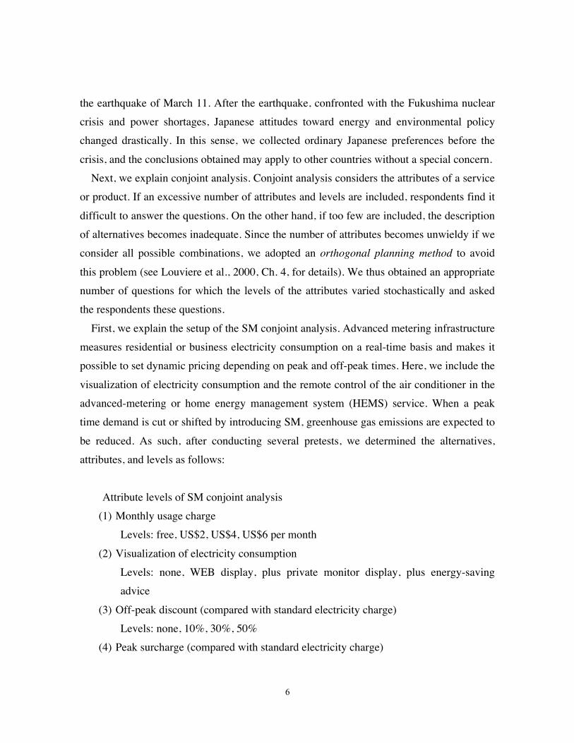
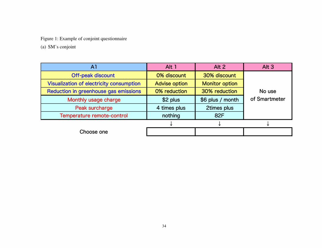
the earthquake of March 11. After the earthquake, confronted with the Fukushima nuclear crisis and power shortages, Japanese attitudes toward energy and environmental policy changed drastically. In this sense, we collected ordinary Japanese preferences before the crisis, and the conclusions obtained may apply to other countries without a special concern. Next, we explain conjoint analysis. Conjoint analysis considers the attributes of a service or product. If an excessive number of attributes and levels are included, respondents find it difficult to answer the questions. On the other hand, if too few are included, the description of alternatives becomes inadequate. Since the number of attributes becomes unwieldy if we consider all possible combinations, we adopted an orthogonal planning method to avoid this problem (see Louviere et al., 2000, Ch. 4, for details). We thus obtained an appropriate number of questions for which the levels of the attributes varied stochastically and asked the respondents these questions. First, we explain the setup of the SM conjoint analysis. Advanced metering infrastructure measures residential or business electricity consumption on a real-time basis and makes it possible to set dynamic pricing depending on peak and off-peak times. Here, we include the visualization of electricity consumption and the remote control of the air conditioner in the advanced-metering or home energy management system (HEMS) service. When a peak time demand is cut or shifted by introducing SM, greenhouse gas emissions are expected to be reduced. As such, after conducting several pretests, we determined the alternatives, attributes, and levels as follows:

Attribute levels of SM conjoint analysis (1) Monthly usage charge

Levels: free, US$2, US$4, US$6 per month (2) Visualization of electricity consumption

Levels: none, WEB display, plus private monitor display, plus energy-saving advice

(3) Off-peak discount (compared with standard electricity charge) Levels: none, 10%, 30%, 50%

(4) Peak surcharge (compared with standard electricity charge)

7

Levels: none, double, four times, six times (5) Remote control of air conditioner during a power shortage

Levels: none, automatic control at 82°F, temporary restriction, usage interception (6) Reduction in greenhouse gas emissions (per household)

Levels: none, 10%, 30%, 50% Figure 1(a) displays an example of the SM conjoint questionnaire. There are three alternatives: Alternatives 1 and 2 denote different SM deployments and Alternative 3 is no SM deployment. All respondents were asked the same eight questions.

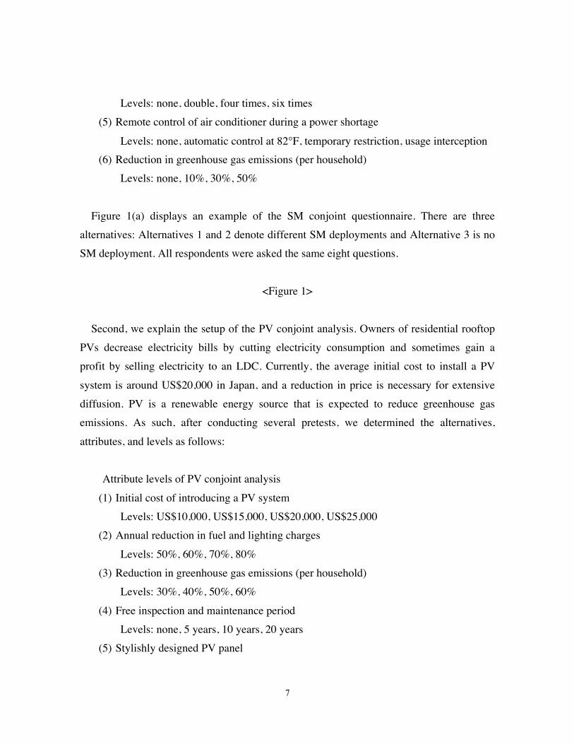
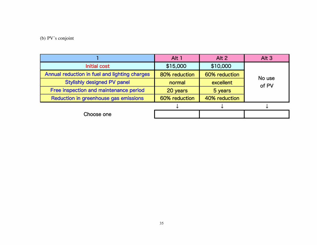
<Figure 1> Second, we explain the setup of the PV conjoint analysis. Owners of residential rooftop PVs decrease electricity bills by cutting electricity consumption and sometimes gain a profit by selling electricity to an LDC. Currently, the average initial cost to install a PV system is around US$20,000 in Japan, and a reduction in price is necessary for extensive diffusion. PV is a renewable energy source that is expected to reduce greenhouse gas emissions. As such, after conducting several pretests, we determined the alternatives, attributes, and levels as follows:

Attribute levels of PV conjoint analysis (1) Initial cost of introducing a PV system

Levels: US$10,000, US$15,000, US$20,000, US$25,000 (2) Annual reduction in fuel and lighting charges

Levels: 50%, 60%, 70%, 80% (3) Reduction in greenhouse gas emissions (per household)

Levels: 30%, 40%, 50%, 60% (4) Free inspection and maintenance period

Levels: none, 5 years, 10 years, 20 years (5) Stylishly designed PV panel

8

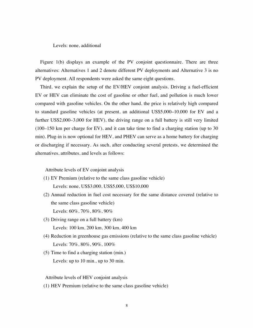
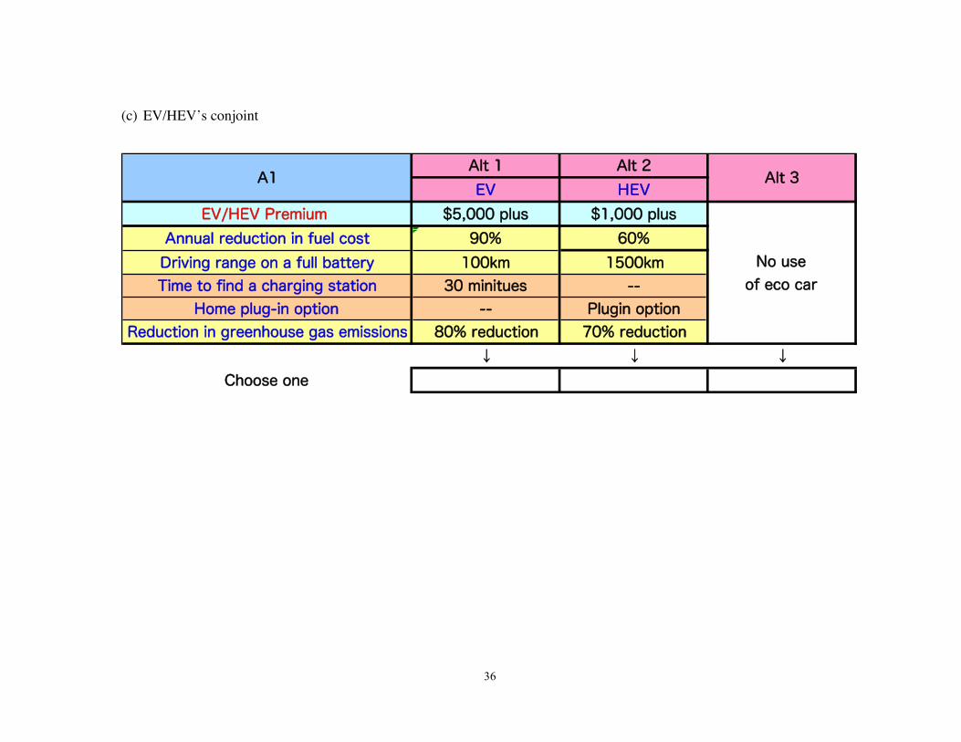
Levels: none, additional Figure 1(b) displays an example of the PV conjoint questionnaire. There are three alternatives: Alternatives 1 and 2 denote different PV deployments and Alternative 3 is no PV deployment. All respondents were asked the same eight questions. Third, we explain the setup of the EV/HEV conjoint analysis. Driving a fuel-efficient EV or HEV can eliminate the cost of gasoline or other fuel, and pollution is much lower compared with gasoline vehicles. On the other hand, the price is relatively high compared to standard gasoline vehicles (at present, an additional US$5,000–10,000 for EV and a further US$2,000–3,000 for HEV), the driving range on a full battery is still very limited (100–150 km per charge for EV), and it can take time to find a charging station (up to 30 min). Plug-in is now optional for HEV, and PHEV can serve as a home battery for charging or discharging if necessary. As such, after conducting several pretests, we determined the alternatives, attributes, and levels as follows:

Attribute levels of EV conjoint analysis (1) EV Premium (relative to the same class gasoline vehicle)

Levels: none, US$3,000, US$5,000, US$10,000 (2) Annual reduction in fuel cost necessary for the same distance covered (relative to

the same class gasoline vehicle) Levels: 60%, 70%, 80%, 90%

(3) Driving range on a full battery (km) Levels: 100 km, 200 km, 300 km, 400 km

(4) Reduction in greenhouse gas emissions (relative to the same class gasoline vehicle) Levels: 70%, 80%, 90%, 100%

(5) Time to find a charging station (min.) Levels: up to 10 min., up to 30 min.

Attribute levels of HEV conjoint analysis

(1) HEV Premium (relative to the same class gasoline vehicle)

9

Levels: none, US$1,000, US$3,000, US$5,000 (2) Annual reduction in fuel cost necessary for the same the distance covered (relative

to the same class gasoline vehicle) Levels: 20%, 40%, 60%, 80%

(3) Driving range before refueling (km) Levels: 700 km, 1,000 km, 1,500 km, 2,000 km

(4) Reduction in greenhouse gas emissions (relative to the same class gasoline vehicle) Levels: 40%, 50%, 60%, 70%

(5) Home plug-in Levels: none, additional

Figure 1(c) displays an example of the EV/HEV conjoint questionnaire. There are three alternatives, where Alternative 1 denotes EV, Alternative 2 denotes HEV, and Alternative 3 is gasoline vehicle purchases. There are sixteen questions in total and they are divided into two versions. All respondents are asked either version (consisting of eight questions) at random.

3. Model specification

This section describes the estimation model. Conditional logit (CL) models, which

assume independent and identical distribution (IID) of random terms, have been widely

used in past studies. However, independence from the irrelevant alternatives (IIA) property

derived from the IID assumption of the CL model is too strict to allow flexible substitution

patterns. A nested logit (NL) model partitions the choice set and allows alternatives to have

common unobserved components compared with non-nested alternatives by partially

relaxing strong IID assumptions. However, the NL model is not suited for our analysis

because it cannot deal with the distribution of parameters at the individual level (Ben-Akiva

et al., 2001). Consequently, the best model for this study is a mixed logit (ML) model,

which accommodates differences in the variance of random components (unobserved

10

heterogeneity). This model is flexible enough to overcome the limitations of CL models by

allowing for random taste variation, unrestricted substitution patterns, and the correlation of

random terms over time (McFadden and Train, 2000).

Assuming that parameter nβ is distributed with density function ( )nf β (Train 2003,

Louviere et al., 2000), the ML specification allows for repeated choices by each sampled

decision maker in such a way that the coefficients vary by person but are constant over each

person’s choice situation. The logit probability of decision maker n choosing alternative i in

choice situation t is expressed as

11( ) [exp( ( )) / exp( ( ))]

T Jnit n nit n njt njtL V Vβ β β

=== ∑∏ , (1)

which is the product of normal logit formulas, given parameter nβ , the observable portion

of utility function nitV , and alternatives j=1, …, J in choice situations t=1, …, T. Therefore,

ML choice probability is a weighted average of logit probability ( )nit nL β evaluated at

parameter nβ with density function ( )nf β , which can be written as

( ) ( )nit nit n n nP L f dβ β β= ∫ . (2)

Accordingly, we can demonstrate variety in the parameters at the individual level using

the maximum simulated likelihood (MSL) method for estimation with a set of 100 Halton

draws1. Furthermore, since each respondent completes eight questions in the conjoint

analysis, the data form a panel, and we can apply a standard random effect estimation.

In the linear-in-parameter form, the utility function can be written as

' 'nit nit n nit nitU x zγ β ε= + + , (3) 1Louviere et al. (2000, p. 201) suggested that 100 replications are normally sufficient for a typical problem involving five alternatives, 1,000 observations, and up to 10 attributes (also see Revelt and Train, 1998). The adoption of the Halton sequence draw is an important issue (Halton, 1960). Bhat (2001) found that 100 Halton sequence draws are more efficient than 1,000 random draws for simulating an ML model.

11

where nitx and nitz denote observable variables, γ denotes a fixed parameter vector,

nβ denotes a random parameter vector, and nitε denotes an independently and identically

distributed extreme value (IIDEV) term.

Because ML choice probability is not expressed in closed form, simulations must be

performed for the ML model estimation. Let θ denote the mean and (co-)variance of

parameter density function ( | )nf β θ . ML choice probability is approximated through the

simulation method (see Train, 2003 p. 148 for details). We can also calculate the estimator

of the conditional mean of random parameter s conditional on individual specific choice

profile ny (see Revelt and Train, 1998 for details), given as

h(β | yn ) = [P( yn |β ) f (β )] / P( yn |β ) f (β )dβ∫ . (4)

From Eq. (4) h(β | yn ) , the conditional choice probabilities P̂nit (βn ) can be calculated individually:

P̂nit (βn ) = exp(Vnit (h(β | yn )) / exp(Vnjt (h(β | yn )))

j=1

J∑ . (5)

After conducting three kinds of conjoint analysis, we expect that a person who has a higher preference for energy conservation is more likely to implement various types of smart equipment, including SM, PV, EV, and HEV. As such, this conjunction leads to a positive interdependency among those choice probabilities. Letting the number of conjoint analysis be m = 1,2,3 , given that the conditional choice probability P̂nit

M=m is influenced by the other conditional choice probabilities P̂nit

M≠m , the random utility function for choosing m can be written as

Unitm = γ 'xnit + βn ' znit + γ n ' P̂nit

M≠m(βn )+ εnit . (6) At this point, parameter γ n indicates interdependencies among the smart equipment

implementations. We will analyze these interdependencies with the utility function shown in Eq. (6) in Section 6.

4. Data description

12

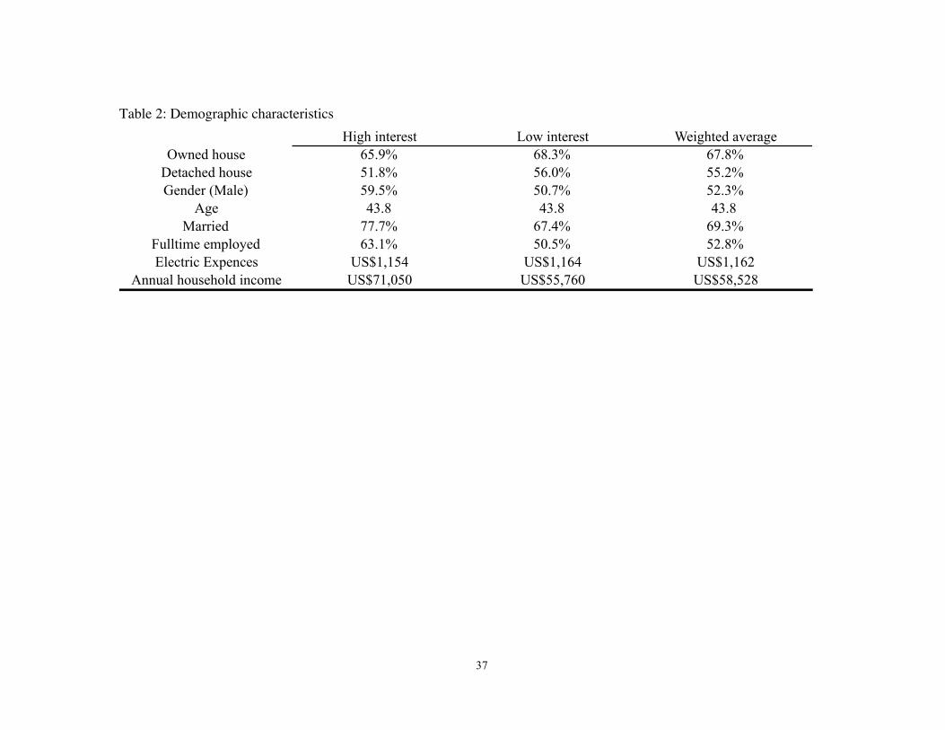
This section discusses the data used for the estimation. Table 2 carries the demographic characteristics of the respondent households; the highly interested households that plan to purchase or remodel a house are shown in the left column, households with little interest are in the center, and the weighted average is shown in the right column. We presently comment on the remarkable difference between the high-interest and the low-interest households.

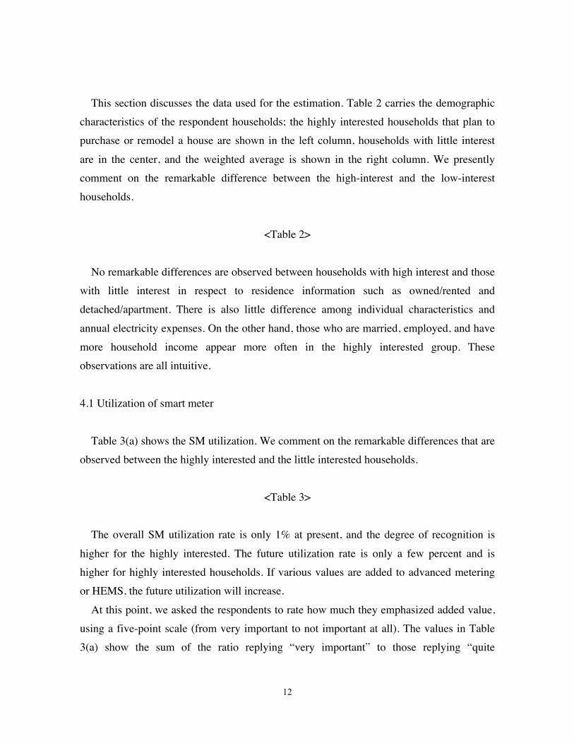
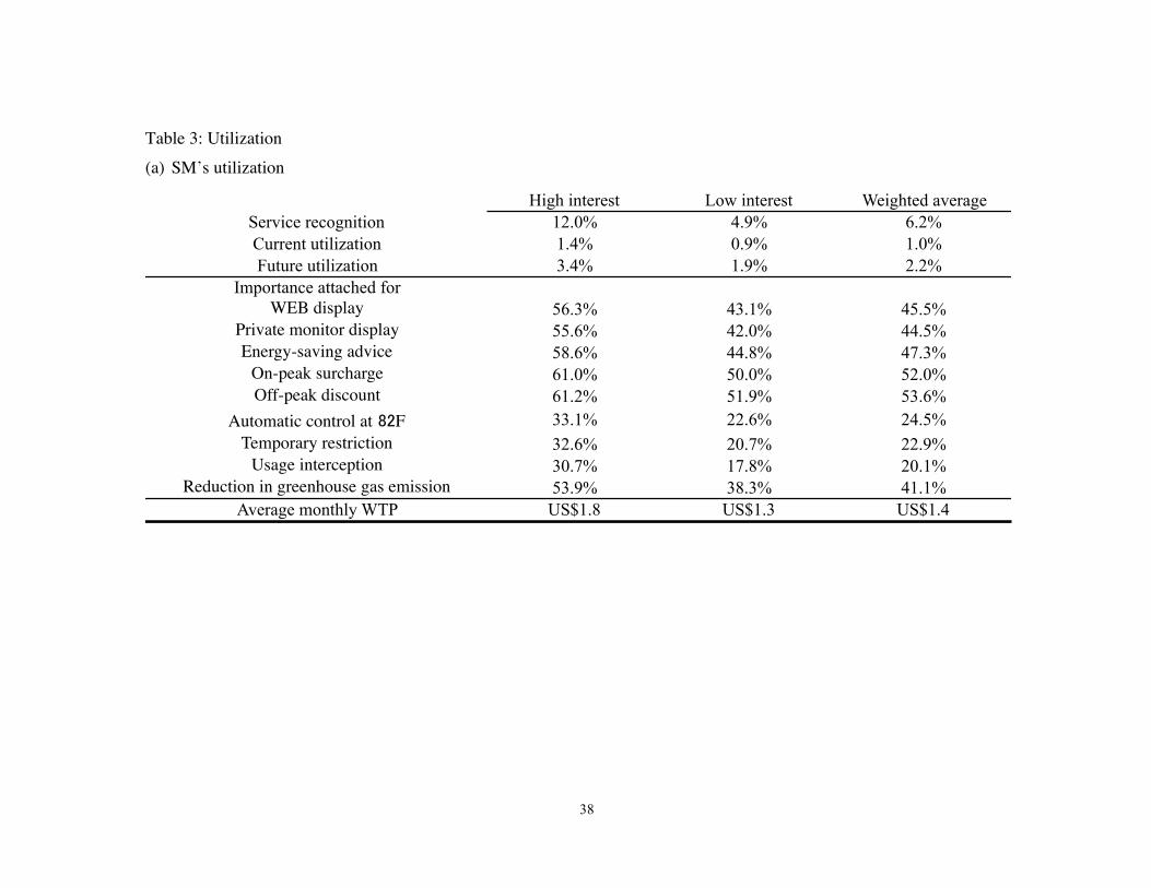
<Table 2> No remarkable differences are observed between households with high interest and those with little interest in respect to residence information such as owned/rented and detached/apartment. There is also little difference among individual characteristics and annual electricity expenses. On the other hand, those who are married, employed, and have more household income appear more often in the highly interested group. These observations are all intuitive. 4.1 Utilization of smart meter Table 3(a) shows the SM utilization. We comment on the remarkable differences that are observed between the highly interested and the little interested households.

<Table 3> The overall SM utilization rate is only 1% at present, and the degree of recognition is higher for the highly interested. The future utilization rate is only a few percent and is higher for highly interested households. If various values are added to advanced metering or HEMS, the future utilization will increase. At this point, we asked the respondents to rate how much they emphasized added value, using a five-point scale (from very important to not important at all). The values in Table 3(a) show the sum of the ratio replying “very important” to those replying “quite

13

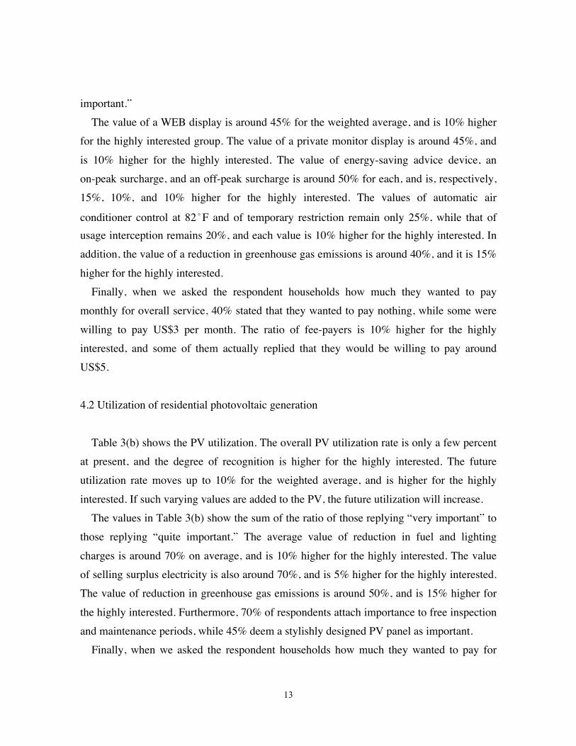
important.” The value of a WEB display is around 45% for the weighted average, and is 10% higher for the highly interested group. The value of a private monitor display is around 45%, and is 10% higher for the highly interested. The value of energy-saving advice device, an on-peak surcharge, and an off-peak surcharge is around 50% for each, and is, respectively, 15%, 10%, and 10% higher for the highly interested. The values of automatic air

conditioner control at 82 F and of temporary restriction remain only 25%, while that of

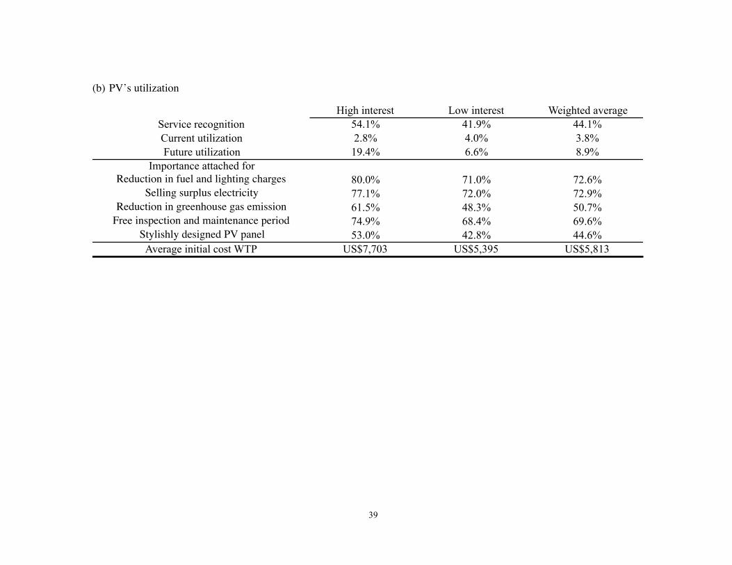
usage interception remains 20%, and each value is 10% higher for the highly interested. In addition, the value of a reduction in greenhouse gas emissions is around 40%, and it is 15% higher for the highly interested. Finally, when we asked the respondent households how much they wanted to pay monthly for overall service, 40% stated that they wanted to pay nothing, while some were willing to pay US$3 per month. The ratio of fee-payers is 10% higher for the highly interested, and some of them actually replied that they would be willing to pay around US$5. 4.2 Utilization of residential photovoltaic generation Table 3(b) shows the PV utilization. The overall PV utilization rate is only a few percent at present, and the degree of recognition is higher for the highly interested. The future utilization rate moves up to 10% for the weighted average, and is higher for the highly interested. If such varying values are added to the PV, the future utilization will increase. The values in Table 3(b) show the sum of the ratio of those replying “very important” to those replying “quite important.” The average value of reduction in fuel and lighting charges is around 70% on average, and is 10% higher for the highly interested. The value of selling surplus electricity is also around 70%, and is 5% higher for the highly interested. The value of reduction in greenhouse gas emissions is around 50%, and is 15% higher for the highly interested. Furthermore, 70% of respondents attach importance to free inspection and maintenance periods, while 45% deem a stylishly designed PV panel as important. Finally, when we asked the respondent households how much they wanted to pay for

14

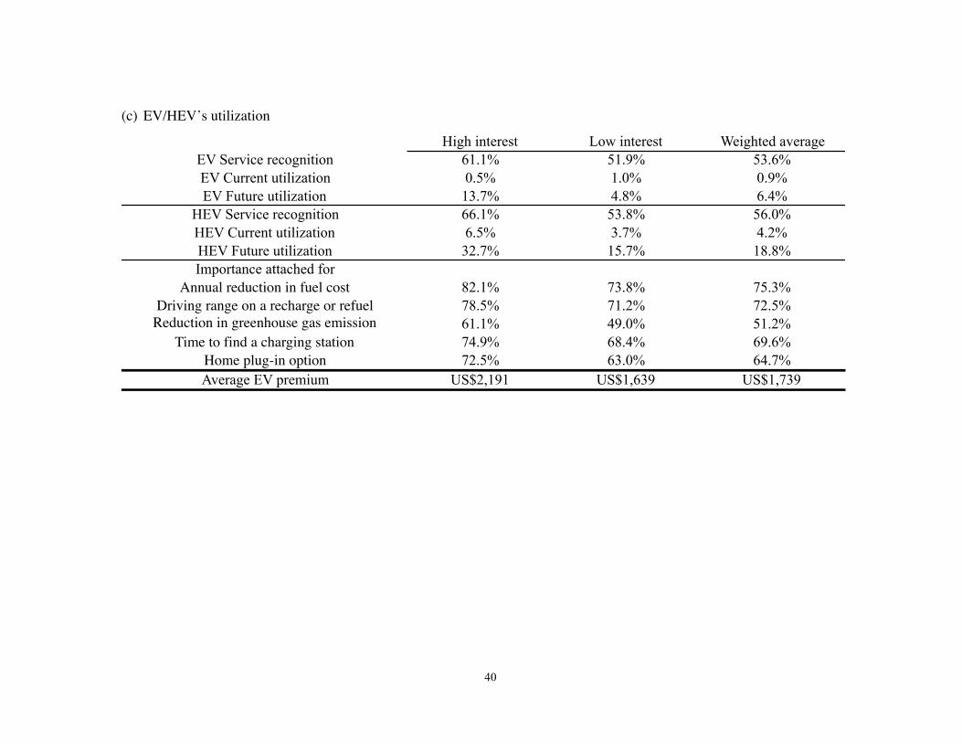
deploying a residential PV system, 25% replied that they would like to pay nothing, while some were willing to pay US$10,000. The ratio of fee-payers is 10% higher for the highly interested, and some of them replied that they would be willing to pay around US$15,000. 4.3 Utilization of electric and hybrid electric vehicles Table 3(c) shows the EV/HEV utilization. The overall EV utilization rate is less than 1% at present, and the degree of recognition is higher for the highly interested. The future utilization rate rises to 10%, and is higher for the highly interested. On the other hand, the overall HEV utilization rate is around several percent at present, and the degree of recognition is higher for the highly interested. The future utilization rate increases to a few tens of percent, and is much higher for the highly interested. The average values in Table 3(c) show the sum of the ratio of those replying “very important” to those replying “quite important.” The value of annual reduction in fuel cost is around 75% on average, and is 10% higher for the highly interested. The value of driving range on a single recharge or refueling is around 70%, and is 10% higher for the highly interested. The value of reduction in greenhouse gas emissions is around 50%, and is 10% higher for the highly interested. Furthermore, 65% of the respondents attach importance to a home plug-in option.

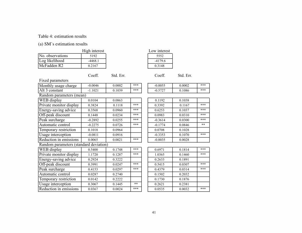
5. Estimation results and analysis This section displays and discusses in order the estimation results of SM, PV, and EV/HEV for both the highly interested households and those with little interest. The number of observations is 5,192 (649 respondents × 8 questions) for the former and 5,552 (694 respondents × 8 questions) for the latter. 5.1 Estimation results for a smart meter Table 4(a) shows the estimation results of the SM conjoint analysis, where the left

15

column displays results for the highly interested and the right column those for the little interested. The McFadden R2 values are 0.2167 for the former and 0.3148 for the latter, both of which are sufficiently high for a discrete choice model. We assume that, except for a monthly usage charge, which is set as a numeraire, the parameters are distributed normally, and the mean and standard deviation values are reported. (Note that *** denotes 1% significance; **, 5% significance; and *, 10% significance.)

<Table 4(a)> First, for the highly interested, the statistically significant estimates (mean) are for monthly usage charge (-), private monitor display (+), energy-saving advice (+), off-peak

discount (+), peak surcharge (-), automatic control at 82 F (-), and reduction in greenhouse

gas emissions (+). Note that the symbols in the parentheses are the signs for each estimate. The statistically significant estimates (standard deviation) are WEB display, private monitor display, off-peak discount, peak surcharge, usage interception, and reduction in greenhouse gas emissions. Next, for those with little interest, the statistically significant estimates (mean) are monthly usage charge (-), private monitor display (+), energy-saving advice (+), off-peak

discount (+), peak surcharge (-), automatic control at 82 F (-), and usage interception (-).

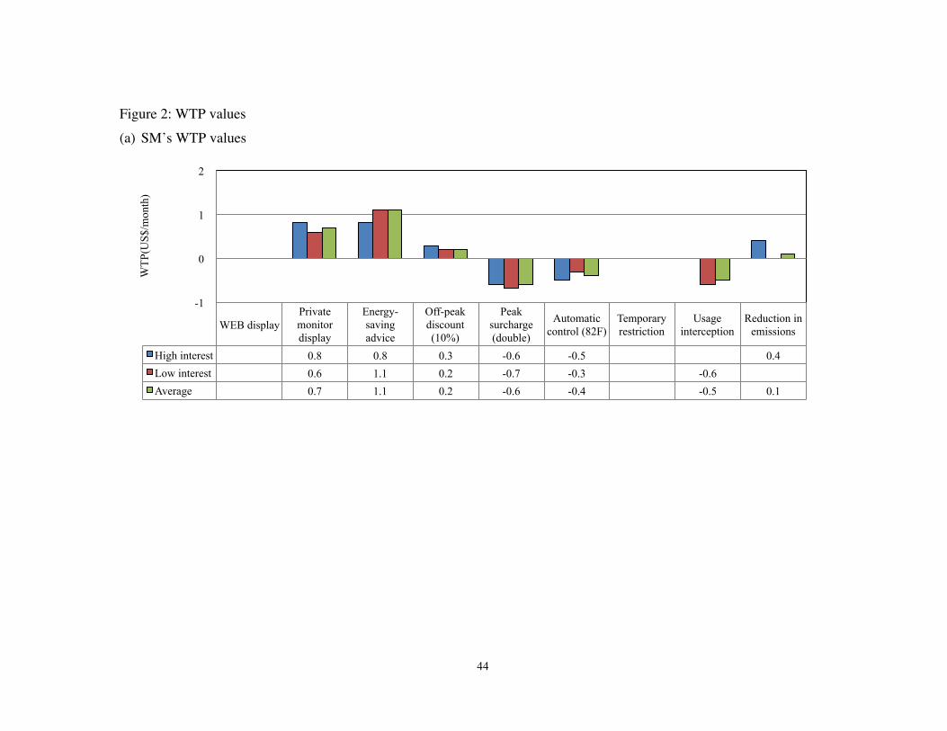
The statistically significant estimates (standard deviation) are WEB display, private monitor display, off-peak discount, peak surcharge, and reduction in greenhouse gas emissions. It follows from the foregoing that the results for the highly interested and those with little interest are similar overall; however, the highly interested have a statistically significant preference for a reduction in greenhouse gas emissions, while the groups with little interest do not. The WTP values are derived from subtracting the parameter of the attribute divided by the numeraire. The WTP values are summarized in Figure 2(a) for the statistically significant attributes. The WTP values are almost the same for the two groups. Note that the average values are close to those for the group with little interest, since the ratio for this

16

group accounts for around 80%.

<Figure 2> At this point, the average WTP values show the positively evaluated items to be a private monitor display (US$0.7/month), energy-saving advice (US$1.1/month), off-peak discount (10%) (US$0.2/month), and reduction in greenhouse gas emissions (10%) (US$0.1/month). On the other hand, items negatively evaluated are peak surcharge (double)

(US$-0.6/month), automatic control at 82 F (US$-0.4/month), and usage interception

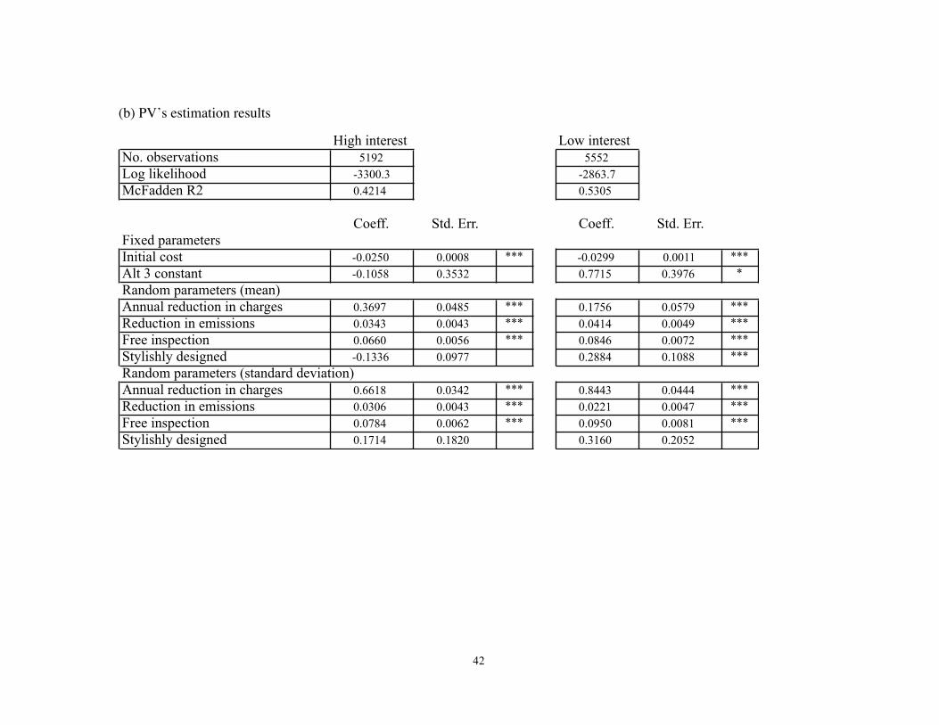
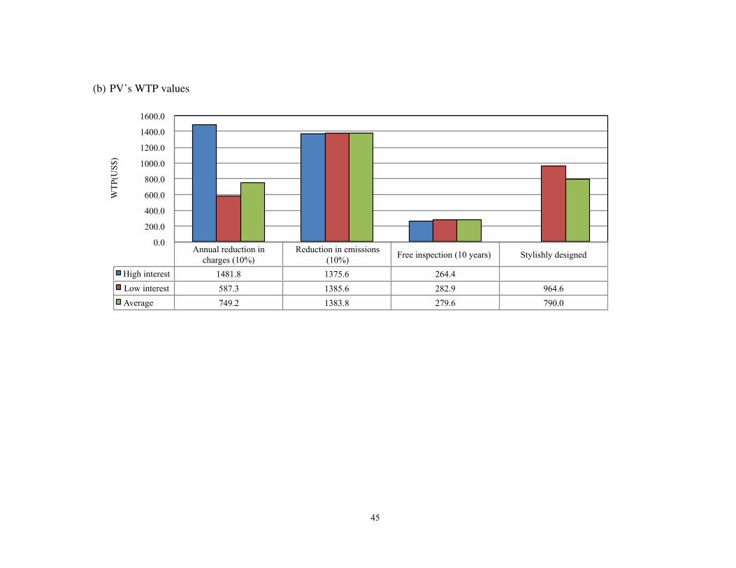
(US$-0.5/month). 5.2 Estimation results of photovoltaic generation Table 4(b) lists the estimation results of the PV conjoint analysis. The McFadden R2 values are 0.4214 for the highly interested and 0.5305 for those with little interest, both of which are very high for a discrete choice model. First, for the highly interested, the statistically significant estimates (mean) are initial cost (-), annual reduction in fuel and lighting charges (+), reduction in greenhouse gas emissions (+), and free inspection and maintenance period (+). The statistically significant estimates (standard deviation) are an annual reduction in fuel and lighting charges, reduction in greenhouse gas emissions, and free inspection and maintenance period. Next, for the group with little interest, the statistically significant estimates (mean) are initial cost (-), annual reduction in fuel and lighting charges (+), reduction in greenhouse gas emissions (+), free inspection and maintenance period (+), and stylishly designed PV panel (+). The statistically significant estimates (standard deviation) are an annual reduction in fuel and lighting charges, reduction in greenhouse gas emissions, and free inspection and maintenance period. The WTP values are summarized in Figure 2(b) for the statistically significant attributes. The two groups show significantly different WTP values. The highly interested group is willing to pay an additional US$1,500 for the initial cost of deploying a PV, and the group

17

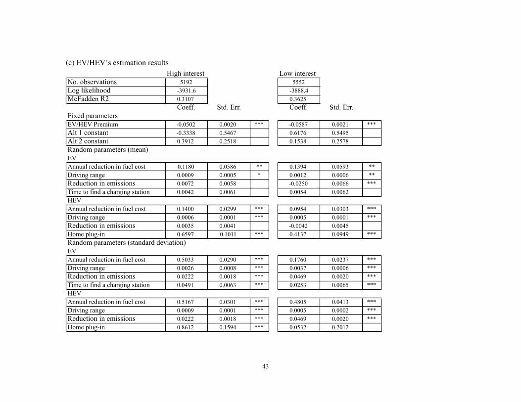
with little interest an additional US$600 to take advantage of a 10% reduction in fuel and lighting charges. That is to say, the highly interested group is relatively sensitive to a reduction in fuel and lighting charges, while the latter group is relatively sensitive to a reduction in initial costs. Note that it is this latter group alone that is willing to pay US$1,000 for a stylishly designed PV panel. Average WTP values in the all households show the positively evaluated items to be an annual reduction in fuel and lighting charges (10%) (US$750), a reduction in greenhouse gas emissions (10%) (US$1,400), free inspection and maintenance period (10 years) (US$300), and a stylishly designed PV panel (US$800). 5.3 Estimation results of electric/hybrid vehicle Table 4(c) lists the estimation results of the EV/HEV conjoint analysis. The McFadden R2 values are 0.3107 for the highly interested and 0.3625 for those with little interest, both of which are sufficiently high for a discrete choice model. First, for the highly interested, the statistically significant estimates (mean) are premium (-) for an EV/HEV, annual reduction in fuel costs (+), and driving range on a full battery (+) for an EV, as well as annual reduction in fuel costs (+), driving range upon refueling (+), and home plug-in (+) for an HEV. The statistically significant estimates (standard deviation) include all parameters for both EV and HEV. Next, for those with little interest, the statistically significant estimates (mean) are premium (-) for an EV/HEV, annual reduction in fuel costs (+),driving range on a full battery (+), and reduction in greenhouse gas emissions (-) for an EV; as well as annual reduction in fuel costs (+), driving range upon refueling (+), and home plug-in (+) for an HEV. The statistically significant estimates (standard deviation) include all parameters for both an EV and HEV, except for a home plug-in for an HEV2.

2 It is counterintuitive that a reduction in greenhouse gas emissions for an EV has a negative sign. One reason for this may be that an EV is a cleaner fuel type vehicle than an HEV, but few respondents chose an EV as an alternative. Consequently, the reduction in

18

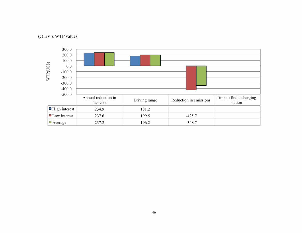
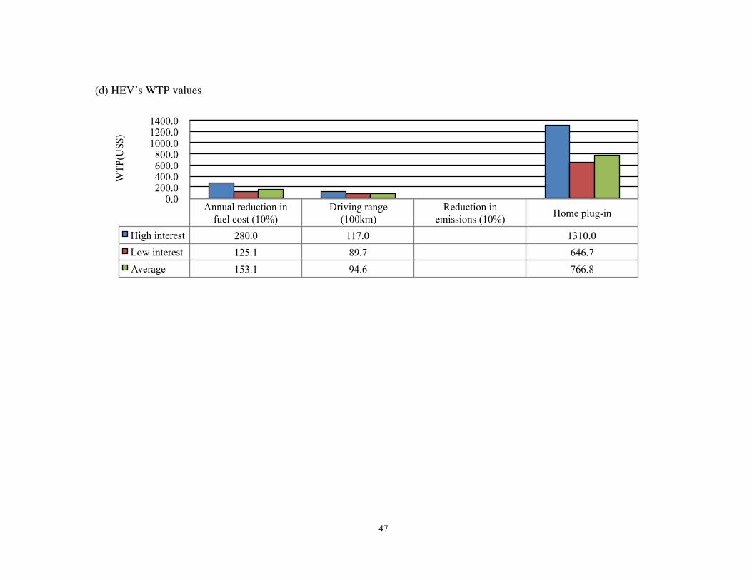
Figures 2(c) and 2(d) summarize the WTP values for the statistically significant attributes. Average WTP values indicate that the items positively evaluated are annual reduction in fuel costs (10%) (US$240) and driving range on a full battery (100 km) (US$200) for an EV3, as well as annual reduction in fuel costs (10%) (US$150), driving range upon refueling (100 km) (US$90), and home plug-in (US$770) for an HEV.

6. Discussions and implications This section discusses the elements of smart-equipment deployment. We begin by calculating the diffusion rates for four different scenarios, and then calculate the reductions in greenhouse gas emissions on the basis of the diffusion rates. We finally investigate the interdependencies of smart-equipment deployments. 6.1 Analysis of diffusion rates We assume two levels for two key attributes (price and greenhouse gas emission reductions) and then calculate the diffusion rates for an SM, PV, EV, and HEV. We first suppose existing standard prices and estimated reductions of greenhouse gas emissions, which were calculated from the available data, to be the default values (see the APPENDIX for details).

Estimated reduction rates of greenhouse gas emissions: Visualization with a smart meter: minus 1.1% per household Peak surcharge (triple): minus 3.7% per household PV deployment: minus 38.2% per household EV deployment: minus 83.5% per car

greenhouse gas emissions of an EV is not associated with a gain in utility. 3 We do not enter into a detailed discussion regarding the unexpected result of emission reduction. See Note 2.

19

HEV deployment: minus 52.4% per car PHEV deployment: minus 64.8% per car

In the following analysis, which is based on a discussion with experts, we also determine the targeted ranges of price and emission reductions for a 5-year period.

6.1.1 Diffusion rates of a smart meter We determine the attribute levels for calculating the SM diffusion rates as follows:

Monthly usage charge: nothing or US$3 Visualization and energy-saving advice Off-peak discount: 50% discount Peak surcharge: triple

Automatic air conditioner control at 82 F

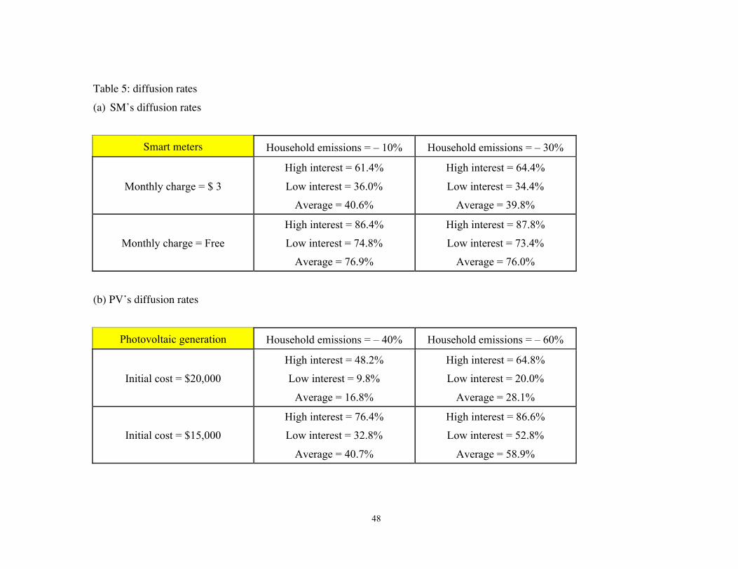
Reduction in greenhouse gas emissions: 10% or 30% We calculated the SM diffusion rates for the highly interested group, those with little interest, and the weighted average of the two groups. The results are listed in Table 5(a). Scenario 1 denotes a combination of [monthly usage charge, reduction in greenhouse gas emissions] = [US$3, 10%]; Scenario 2, [US$0, 10%]; Scenario 3, [US$3, 30%]; and Scenario 4, [US$0, 30%]. Therefore, for consumers, Scenario 1 is the worst and Scenario 4 is the best. In Scenario 1, the diffusion rates are 61.4% for the highly interested, 36.0% for those with little interest, and 40.6% for the average between the two. On the other hand, in Scenario 4, the diffusion rates are 87.8% for the highly interested, 73.4% for the little interested, and 76.0% for the average. Note again that the average figure is closer to that for the group with little interest, as this group accounts for around 80% of the respondents. Furthermore, comparisons of Scenarios 1 and 2, and Scenarios 3 and 4 reveal the differences to be more than 30% for the average. These become much larger for those with

20

little interest, as the latter are so sensitive to price that they are willing to introduce smart meters for free. On the other hand, few differences are observed when comparing Scenarios 1 and 3, and Scenarios 2 and 4. This is because the highly interested have a very small, though statistically significant, preference for a reduction in greenhouse gas emissions, while the group with little interest does not have a statistically significant preference. In short, the free charge policy is very effective, but the incentive of a decrease in greenhouse gas emissions is less effective for the spreading of a smart meter infrastructure.

<Table 5>

6.1.2 Diffusion rates of residential photovoltaic generation We determine the attribute levels for calculating the PV diffusion rates as follows:

Initial cost: US$15,000 or US$20,000 Annual reduction in fuel and lighting charges: 60% Reduction in greenhouse gas emissions: 40% or 60% Free inspection and maintenance period: 10 years Stylishly designed PV panel

The PV diffusion rates are listed in Table 5(b). Scenario 1 denotes a combination of [initial cost, reduction in greenhouse gas emissions] = [US$20,000, 40%]; Scenario 2, [US$15,000, 40%]; Scenario 3, [US$20,000, 60%]; and Scenario 4, [US$15,000, 60%]. In Scenario 1, the diffusion rates are 48.2% for the highly interested, 9.8% for those little interested, and 16.8% for the average between them. On the other hand, in Scenario 4, the diffusion rates are 86.6% for the highly interested, 52.8% for the group with little interest, and 58.9% for the average. As expected, the gaps between the two groups are very large. Furthermore, comparisons of Scenarios 1 and 2, and Scenarios 3 and 4 reveal the average differences between the two groups to be around 20 to 30%. This means that the current initial cost is around US$20,000, but this must be decreased to US$15,000 to encourage

21

further PV diffusion. On the other hand, comparisons of Scenarios 1, and 3 and Scenarios 2 and 4 highlight gaps of 10 to 20%. We, therefore, see that a reduction in greenhouse gas emissions works as a strong motivation for PV deployment, which is very unlike the case of a smart meter. The reason the effects of emission reduction incentives vary depending on appliances is ambiguous. One possible answer is that consumers care about the process of reducing greenhouse gas emissions, but the process of reducing emissions by means of a PV is more explicit than that of an SM. Accordingly, a reduction in greenhouse gas emissions is effective in PV deployment. The effects of emission reduction incentives on diffusion rates might depend on the consumer “literacy” regarding smart equipment. Note that PVs for households have been sold in Japan for more than a decade. The initial cost of introducing a PV into a household is considerable (up to $20,000). Thus, PV manufacturers and sellers in Japan have been making every effort to advertise several appealing aspects of PV, specifically its powerful ability to reduce greenhouse gas emissions, in addition to its helping reduce annual fuel and lighting charges. As a result, Japanese consumers have become increasingly aware of the ability of PV to reduce greenhouse gas emissions. In contrast, SM and PHEV have not even been sold in Japan as yet. The effects of emission reduction incentives on diffusion rates may increase if there is an increase in consumer “literacy” regarding types of smart equipment, such as PHEV, after these are introduced into the market in the near future.

6.1.3 Diffusion rates of electric and plug-in hybrid electric vehicles We determine the attribute levels for calculating the EV/PHEV diffusion rates as follows:

EV EV premium: US$5,000 or US$10,000 Annual reduction in fuel cost: 80% Driving range on a full battery: 200 km

Reduction in greenhouse gas emissions: 80% or 100％

22

Time to find a charging station: within 10 min. PHEV HEV premium: US$2,500 or US$5,000 Annual reduction in fuel costs: 60% Driving range on a full battery: 1,500 km

Reduction in greenhouse gas emissions: 60% or 80％ Home plug-in

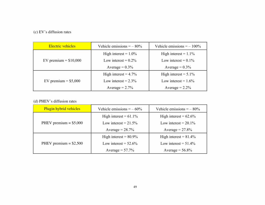
Tables 5(c) and (d) list the EV and PHEV diffusion rates, respectively. For an EV, Scenario 1 denotes a combination of [EV premium, reduction in greenhouse gas emission] = [US$10,000, 80%]; Scenario 2, [US$5,000, 80%]; Scenario 3, [US$10,000, 100%]; and Scenario 4, [US$5,000, 100%]. On the other hand, for PHEV, Scenario 1 denotes a combination of [PHEV premium, reduction in greenhouse gas emission] = [US$5,000, 60%]; Scenario 2, [US$2,500, 60%]; Scenario 3, [US$5,000, 80%]; and Scenario 4, [US$2,500, 80%]. In Scenario 1, the EV diffusion rates are 1.0% for the highly interested, 0.2% for those with little interest, and 0.3% for the average between the two groups; the PHEV diffusion rates are 61.1% for the highly interested, 21.5% for those with little interest, and 28.7% for the average. On the other hand, in Scenario 4, the EV diffusion rates are 5.1% for the highly interested, 1.6% for those with little interest, and 2.2% for the average; while the PHEV diffusion rates are 81.4% for the highly interested, 51.4% for the little interested, and 56.8% for the average. It is important to note that the gaps between the EV and the PHEV diffusion rates are extremely large. One possible reason for the significantly low rates of EV’s diffusion might be its limited driving range. The EV’s driving range on a full battery is currently much lower than the driving range of a standard gasoline engine car, whereas the EV premium is quite high. Technological innovations that decrease production costs and enable a much longer driving range would enhance the future diffusion of EVs. Furthermore, comparisons of Scenarios 1 and 2, and Scenarios 3 and 4 show that even if the EV premium decreases from US$10,000 to US$5,000, the EV diffusion rates do not

23

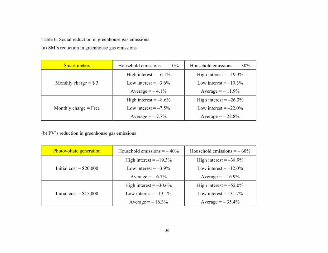
drastically increase. On the other hand, if the PHEV premium decreases from US$5,000 to US$2,500, the PHEV diffusion rates double. We might say that a premium approaching less than US$5,000 is necessary for the full-scale deployment of electric vehicles (especially PHEV). On the other hand, as with the diffusion of smart meters, a reduction in greenhouse gas emissions does not have an influence on EV deployment, even though we may expect a large reduction in greenhouse gas emissions by driving EVs. Since the clean efficiency of a PHEV now compares favorably with that of an EV, however, the difference in the emission reduction is neither distinct nor critical for the respondents. There has, as yet, been no full-scale sale of EV and PHEV. As discussed before, the effects of emission reduction incentives on diffusion rates could increase if there is an increase in consumer “literacy” regarding those vehicles in the near future. 6.2 Analysis of reduction in greenhouse gas emission Here, we analyze the social reductions in greenhouse gas emissions that are calculated from the diffusion rates discussed in Section 6.1. The social reductions are derived as follows. The highly interested reduction rate of greenhouse gas emission = highly interested

diffusion rate × estimated reduction rates The little interested reduction rate of greenhouse gas emission = little interested

diffusion rate × estimated reduction rates The expected social reduction rate of greenhouse gas emission = 0.181 × highly

interested reduction rate + 0.819 × little interested reduction rate Table 6 lists the expected social reduction rates of greenhouse gas emissions for smart equipment. The definitions of the scenarios shown were given in the previous section.

<Table 6>

24

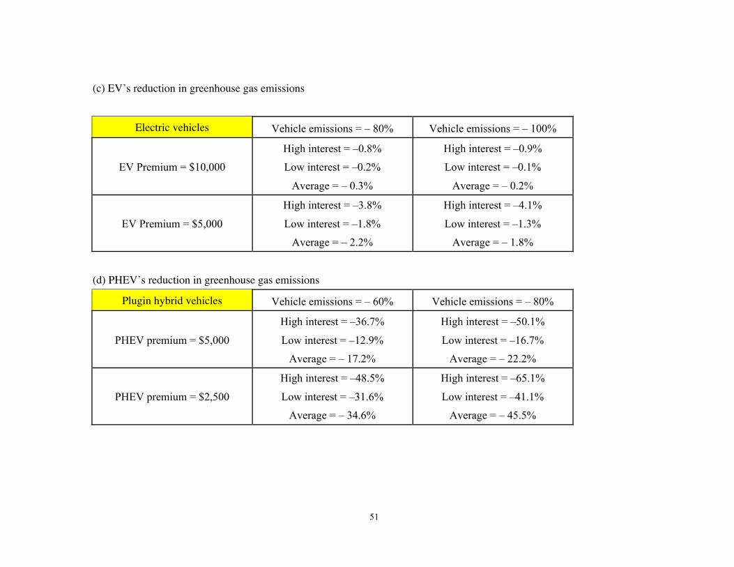
First, for the SM social reduction rate (per household), the values resulting from Scenario 1 (the worst) are 6.1% for the highly interested, 3.6% for those with little interest, and 4.1% for the average between the two groups. On the other hand, the values resulting from Scenario 4 (the best) are 26.3% for the highly interested, 22.0% for the little interested, and 22.8% for the average. Second, for the PV social reduction rate (per household), the values resulting from Scenario 1 are 19.3% for the highly interested, 3.9% for those with little interest, and 6.7% for the average. On the other hand, the values resulting from Scenario 4 are 52.0% for the highly interested, 31.7% for the little interested, and 35.4% for the average. Third, for the EV social reduction rate (per car), the values resulting from Scenario 1 are 0.8% for the highly interested, 0.2% for the little interested, and 0.3% for the average. On the other hand, the values resulting from Scenario 4 are 4.1% for the highly interested, 1.3% for the little interested, and 1.8% for the average. Fourth, for the PHEV social reduction rate (per car), the values resulting from Scenario 1 are 36.7% for the highly interested, 12.9% for the little interested, and 17.2% for the average. On the other hand, the values resulting from Scenario 4 are 65.1% for the highly interested, 41.1% for the little interested, and 45.5% for the average. To summarize, by the diffusion of smart equipment, a social reduction in greenhouse gas emissions is extensively advanced. Assuming the present standard scenario, the reductions are estimated to be 4% for SM, 7% for PV, and 17% for PHEV. If we add some innovations to the equipment, larger reductions would be expected. The social reductions in greenhouse gas emissions depend on the balance of the diffusion rate of smart equipment and the individual reduction rate of greenhouse gas emissions. SM has a much lower individual reduction rate of greenhouse gas emissions than PV, whereas the diffusion rate of SM is higher than that of PV. Consequently, the difference between SM and PV in terms of the social reductions is not so large. The EV’s social reductions are significantly small because its diffusion rate is extremely low. In contrast, PHEV’s diffusion rate and individual reduction rate of greenhouse gas emissions are somewhat balanced, which results in a relatively great amount of social reductions for PHEV.

25

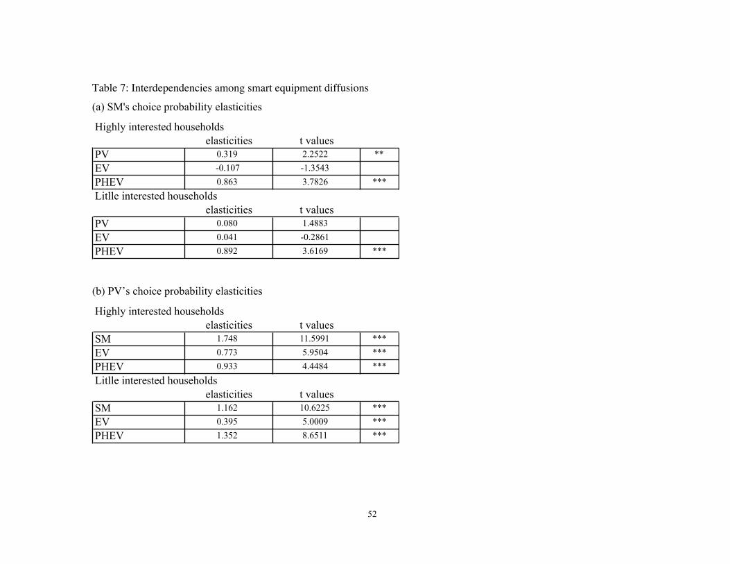
6.3 Analysis of interdependencies among smart equipment diffusion We have thus far analyzed three different conjoint studies separately. However, there are interdependencies among consumer preferences for smart equipment used in a smart home. For example, a consumer who is interested in a PHEV is likely to receive a time-of-use electricity price by using an SM, whereas a household that installs a residential PV may consider a PHEV as a convenient home battery. We try to ascertain these interdependencies by inserting other choice probabilities depicted in Eq. (6) into the estimation equation of certain smart equipment as explanatory variables. Table 7 lists the main estimation results (selectively, the choice probability parameters) for those with high and little interest, respectively. The estimates are transformed into elasticities, which indicate how much a percentage increase in a choice probability increases another choice probability. Note that the values in the parentheses are t values: *** denotes 1% significant; **, 5% significant; and *, 10% significant. We adopted an orthogonal planning method in establishing the questionnaire, and therefore, the correlation is eliminated among explanatory variables. Thus, the introduction of expected choice probabilities has almost no influence on the estimates of the conjoint attributes, and we have verified that the estimation results remain very robust.

<Table 7> First, for the SM estimation results (choice probability elasticities), the statistically significant items are PV (0.319**) and PHEV (0.863***) for the highly interested, and PHEV (0.892***) for the little interested. We can therefore see that PHEVs will be a driving force for the choice of an SM. Note, however, that here we show not causality but correlation. Several interpretations are allowed. For example, with PHEV diffusion, the economic value of introducing an SM increases; or, only households that have already installed an SM are willing to purchase a PHEV. Next, for the PV estimation results, the statistically significant items are SM (1.748***);

26

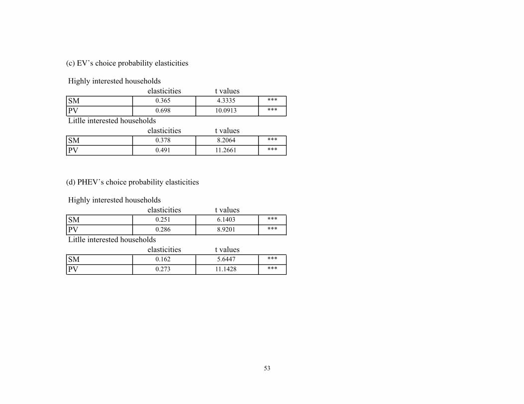
EV (0.773***); and PHEV (0.933***) for the highly interested, and SM (1.162***), EV (0.395***), and PHEV (1.352***) for those with little interest. All smart equipment influences PV adoption, and the effects of SM and PHEV are sometimes elastic. These results may reflect the fact that early adopters who deploy residential PV systems have high environmental consciousness. PV is also considered a hopeful renewable energy source and explicitly contributes to the reduction in greenhouse gas emissions. Finally, for the EV estimation results, the statistically significant items are SM (0.365***) and PV (0.698***) for the highly interested, and SM (0.378***) and PV (0.491***) for the group with little interest. On the other hand, for the PHEV estimation results, the statistically significant items are SM (0.251***) and PV (0.286***) for those with high interest, and SM (0.162***) and PV (0.273***) for those with little interest. We see that the preferences for an EV/PHEV are associated with the other smart equipment deployments. This is partially because an EV/PHEV serves as a home battery, which alleviates the problem of an unstable power supply associated with a renewable energy source. To summarize, the choice behaviors for smart equipment are not independent and they reinforce the purchases of other smart equipment. Therefore, an incentive policy that induces consumers to purchase smart equipment simultaneously should be considered.

7. Concluding remarks This paper conducted three kinds of conjoint analysis studies using a mixed logit model on the basis of an online survey carried out in March of 2011. First, we examined the WTP values for the attributes of smart equipment. Furthermore, we investigated the diffusion rates, the reduction in greenhouse gas emissions, and interdependencies among the smart equipment deployments. We obtained the following conclusions. First, a decrease in price is the most effective promotion for smart equipment deployments. On the other hand, the effects varied across the different types of equipment for the reduction in greenhouse gas emissions, although it was highest for PV deployment. The effects of emission reduction incentives may also depend on the consumer “literacy” regarding smart equipment. Second,

27

with smart equipment diffusion, greenhouse gas emissions would be reduced in society. According to the standard scenario, the reduction rates were 4% for SM, 7% for PV, and 17% for PHEV. Innovation will enlarge these reductions in the future. Third, interdependencies among the different types of smart equipment deployments were observed, and PV deployment is particularly associated with all other equipment deployments. As a final remark, we acknowledge that all of these results are based on a data analysis of stated preference, which must be reconfirmed using a revealed preference data analysis in the future. The results of such an analysis remain an important question for the future.

28

Appendix

In Japan, an average household emits 3216kg of CO2 annually by consuming electricity

(4500kWh) and gas (600m3) (Central Research Institute of Electric Power Industry:

CRIEPI, Ministry of Internal Affairs and Communications: MIC). The CO2 emission rates

of the electric power companies when generating power are 0.44kg-CO2/kWh in the

daytime, 0.39kg-CO2/kWh in the nighttime, and 0.42kg-CO2/kWh on average (CRIEPI,

Minister of Economy, Trade and Industry: METI, Ministry of Environment: MOE).

Visualization with a smart meter

Introduction of a smart meter and private monitor display reportedly reduced the

electricity use of an average household by 1.8% (New Energy and Industrial Technology

Development Organization: NEDO, Mitsubishi Research Institute: MRI). This corresponds

to an annual reduction in electricity usage by 81kWh and in CO2 emissions by 34kg-CO2

per household, when applying the average CO2 emission rate. Thus, the reduction rate of

CO2 is 1.1％ (34/3216kg-CO2) per household.

Peak surcharge

Faruqui et al. (2010) reported that the price elasticity of electricity demand ranges from

0.073 to 0.13 by surveying the existing demand response (DR) programs in U.S. We here

assume that the price elasticity of electricity demand is 0.1. When the electricity tariff

during the peak period is tripled, a household will reduce its electricity usage by 270kWh

per year (in relation to the annual electricity usage in the peak period defined in the TOU

tariff, i.e., 1350kWh; METI). This amounts to an annual reduction in CO2 emissions of

119kg-CO2, when applying the CO2 emission rate in the daytime. Thus, the reduction rate

of CO2 is 3.7％ (119/3216kg-CO2) per household.

PV deployment

The power output of home solar PV is 3kW on average, which generates 3000kWh of

electricity annually (National Institute of Advanced Industrial Science and Technology:

29

AIST). This leads to an annual reduction in CO2 emissions by 1230kg-CO2, when applying

the CO2 emission rate in the daytime (CO2 emissions caused in the process of producing

PV panels is deducted, i.e., 0.44kg-CO2/kWh − 0.03kg-CO2/kWh). Thus, the reduction

rate of CO2 is 38.2％ (1230/3216kg-CO2) per household.

In Japan, the average annual travel distance of a gasoline engine car is 9188km (Ministry

of Land, Infrastructure, Transport, and Tourism: MLIT). The annual CO2 emissions

amount to 2345kg-CO2 per car, based on the fuel efficiency of 9.1km/L and CO2 emission

rate of 2.32 kg-CO2/L (MLIT).

EV deployment

The electric efficiency of EV is estimated to be 10.0km/kWh (METI). Based on this

estimate, the annual reduction in CO2 emissions is 1959kg-CO2 per car. Thus, the

reduction rate of CO2 is 83.5％ (1959/2345kg-CO2) per car.

HEV deployment

The fuel efficiency of HEV is 19.1km/L (Toyota and Honda). Based on this estimate, the

annual reduction in CO2 emissions is 1228kg-CO2 per car. Thus, the reduction rate of CO2

is 52.4％ (1228/2345kg-CO2) per car.

PHEV deployment

The PHEV is estimated to run with gasoline for 60% and with electric power for 40% of

the travel distance (METI). Based on this estimate, the annual reduction in CO2 emissions

is 1520kg-CO2 per car. Thus, the reduction rate of CO2 is 64.8％ (1520/2345kg-CO2) per

car.

30

References [1] Ahn, J., Jeong, G., Kim, Y., 2008. A forecast of household ownership and use of

alternative fuel vehicles: A multiple discrete-continuous choice approach. Energy Economics 30. 2091-2104.

[2] Axsen, J., Mountain, D.C., Jaccard, M., 2009. Combining stated and revealed choice research to simulate the neighbor effect: The case of hybrid-electric vehicles. Resource and Energy Economics 31, 221-238.

[3] Banfi, S., Farsi, M., Filippini, M., Jakob, M., 2008. Willingness to pay for energy-saving measures in residential buildings. Energy Economics 30, 503-516.

[4] Beggs, S., Cardell, S., Hausman, J., 1981. Assessing the Potential Demand for Electric Cars. Journal of Econometrics 16, 1–19.

[5] Ben-Akiva, M., Bolduc D., Walker J., 2001. Specification, estimation and identification of the logit kernel (or continuous mixed logit) model. Department of Civil Engineering, MIT, Working Paper.

[6] Bhat, C., 2001. Quasi-random maximum simulated likelihood estimation of the mixed multinomial logit model. Transportation Research B35, 677-693.

[7] Brownstone, D., Train, K.E., 1999. Forecasting new product penetration with flexible substitution patterns. Journal of Econometrics 89, 109-129.

[8] Brownstone, D., Bunch, D.S., Train, K.E., 2000. Joint mixed logit models of stated and revealed preferences for alternative-fuel vehicles. Transportation Research B34, 315-338.

[9] Bunch, D.S., Bradley, M., Golob, T.F., Kitamura, R., Occhiuzzo, G.P., 1993. Demand for clean-fuel vehicles in California: A discrete-choice stated preference pilot project. Transportation Research A27 (3), 237-253.

[10] Calfee, J.E., 1985. Estimating the demand for electric automobiles using disaggregated probabilistic choice analysis. Transportation Research B: Methodological 19 (4), 287–301.

[11] Clastres, C., 2011. Smart grids: Another step towards competition, energy security and climate change objectives. Energy Policy, DOI: 10.1016/j.enpol.2011.05.024.

31

[12] Dagsvike, J.K., Wetterwald, D.G., Wennemo, T., Aaberge, R., 2002. Potential demand for alternative fuel vehicles. Transportation Research Part B: Methodological 36, 361–384.

[13] Duke, R., Williams, R., Payne, A., 2005. Accelerating residential PV expansion: demand analysis for competitive electricity markets. Energy Policy 33, 1912-1929.

[14] Ewing G., Sarigollu, E., 2000. Assessing consumer preferences for clean-fuel vehicles: A discrete choice experiment. Journal of Public Policy & Marketing 19 (1), 106-118.

[15] Faruqui, A., Hledik, R., Sergici S., 2010. Rethinking Prices: The changing architecture of demand response in America. Public Utilities Fortnightly, January.

[16] Halton, J.E., 1960. On the efficiency of certain quasi-random sequences of points in evaluating multi-dimensional integrals. Numerische Mathematik 2, 84-90.

[17] Hidrue, M.K., Parsons, G.R., Kempton, W., Gardner, M.P., 2011. Willingness to pay for electric vehicles and their attributes. Resource and Energy Economics 33, 686-705.

[18] Karplus, V.J., Paltsev, S., Reilly, J.M., 2010. Prospects for plug-in hybrid electric vehicles in the United States and Japan: A general equilibrium analysis. Transportation Research A44, 620-641.

[19] Keirstead, J., 2007. Behavioural responses to photovoltaic systems in the UK domestic sector. Energy Policy 35, 4128-4141.

[20] Louviere, J.J., Hensher D.A., Swait J.D., 2000. Stated choice methods: analysis and applications. Cambridge University Press.

[21] McFadden, D., Train K.E., 2000. Mixed MNL models of discrete choice models of discrete response. Journal of Applied Econometrics 15, 447-470.

[22] Mau, P., Eyzaguirre, J., Jaccard, M., Collins-Dodd, C., Tiedemann, K., 2008. The ‘neighbor effect’: Simulating dynamics in consumer preferences for new vehicle technologies. Ecological Economics 68, 504-516.

[23] Potoglou, D., Kanaroglou, P.S., 2007. Household demand and willingness to pay for clean vehicles. Transportation Research D12, 264-274.

[24] Revelt, D., Train K.E., 1998. Mixed logit with repeated choices: Households' choices of appliance efficiency level. Review of Economics and Statistics 80, 647-657.

32

[25] Segal, R., 1995. Forecasting the Market for Electric Vehicles in California Using Conjoint Analysis. The Energy Journal 16 (3), 89-111.

[26] Train, K.E., 2003. Discrete Choice Methods with Simulation. Cambridge University Press.

[27] Woo, C.K., Kollman, E., Orans, R., Price, S., Horii, B., 2008. Now that California has AMI, what can the state do with it? Energy Policy 36, 1366-1374.

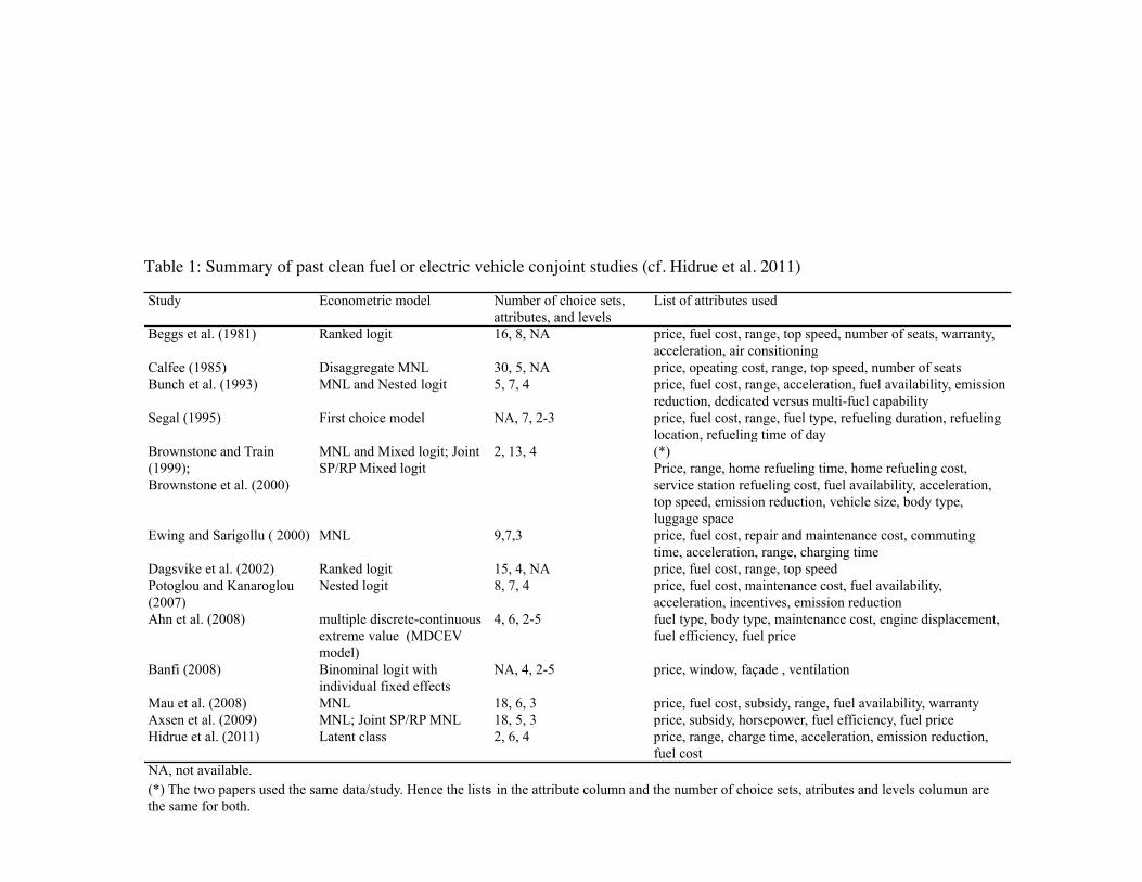
Table 1: Summary of past clean fuel or electric vehicle conjoint studies (cf. Hidrue et al. 2011)

Study Econometric model Number of choice sets,attributes, and levels

List of attributes used

Beggs et al. (1981) Ranked logit 16, 8, NA price, fuel cost, range, top speed, number of seats, warranty,acceleration, air consitioning

Calfee (1985) Disaggregate MNL 30, 5, NA price, opeating cost, range, top speed, number of seatsBunch et al. (1993) MNL and Nested logit 5, 7, 4 price, fuel cost, range, acceleration, fuel availability, emission

reduction, dedicated versus multi-fuel capabilitySegal (1995) First choice model NA, 7, 2-3 price, fuel cost, range, fuel type, refueling duration, refueling

location, refueling time of dayBrownstone and Train(1999);Brownstone et al. (2000)

MNL and Mixed logit; JointSP/RP Mixed logit

2, 13, 4 (*)Price, range, home refueling time, home refueling cost,service station refueling cost, fuel availability, acceleration,top speed, emission reduction, vehicle size, body type,luggage space

Ewing and Sarigollu ( 2000) MNL 9,7,3 price, fuel cost, repair and maintenance cost, commutingtime, acceleration, range, charging time

Dagsvike et al. (2002) Ranked logit 15, 4, NA price, fuel cost, range, top speedPotoglou and Kanaroglou(2007)

Nested logit 8, 7, 4 price, fuel cost, maintenance cost, fuel availability,acceleration, incentives, emission reduction

Ahn et al. (2008) multiple discrete-continuousextreme value (MDCEVmodel)

4, 6, 2-5 fuel type, body type, maintenance cost, engine displacement,fuel efficiency, fuel price

Banfi (2008) Binominal logit withindividual fixed effects

NA, 4, 2-5 price, window, façade , ventilation

Mau et al. (2008) MNL 18, 6, 3 price, fuel cost, subsidy, range, fuel availability, warrantyAxsen et al. (2009) MNL; Joint SP/RP MNL 18, 5, 3 price, subsidy, horsepower, fuel efficiency, fuel priceHidrue et al. (2011) Latent class 2, 6, 4 price, range, charge time, acceleration, emission reduction,

fuel costNA, not available.(*) The two papers used the same data/study. Hence the list in the attribute column and the number of choice sets, atributes and levels columun arethe same for both.

34

Figure 1: Example of conjoint questionnaire (a) SM’s conjoint

AA11 AAlltt 11 AAlltt 22 AAlltt 33OOffff--ppeeaakk ddiissccoouunntt 00%% ddiissccoouunntt 3300%% ddiissccoouunntt

VViissuuaalliizzaattiioonn ooff eelleeccttrriicciittyy ccoonnssuummppttiioonn AAddvviissee ooppttiioonn MMoonniittoorr ooppttiioonnRReedduuccttiioonn iinn ggrreeeennhhoouussee ggaass eemmiissssiioonnss 00%% rreedduuccttiioonn 3300％％ rreedduuccttiioonn

MMoonntthhllyy uussaaggee cchhaarrggee $$22 pplluuss $$66 pplluuss // mmoonntthhPPeeaakk ssuurrcchhaarrggee 44 ttiimmeess pplluuss 22ttiimmeess pplluuss

TTeemmppeerraattuurree rreemmoottee--ccoonnttrrooll nnootthhiinngg 8822FF↓↓ ↓↓ ↓↓

CChhoooossee oonnee

NNoo uusseeooff SSmmaarrttmmeetteerr

35

(b) PV’s conjoint

11 AAlltt 11 AAlltt 22 AAlltt 33IInniittiiaall ccoosstt $$1155,,000000 $$1100,,000000

AAnnnnuuaall rreedduuccttiioonn iinn ffuueell aanndd lliigghhttiinngg cchhaarrggeess 8800%% rreedduuccttiioonn 6600%% rreedduuccttiioonnSSttyylliisshhllyy ddeessiiggnneedd PPVV ppaanneell nnoorrmmaall eexxcceelllleenntt

FFrreeee iinnssppeeccttiioonn aanndd mmaaiinntteennaannccee ppeerriioodd 2200 yyeeaarrss 55 yyeeaarrssRReedduuccttiioonn iinn ggrreeeennhhoouussee ggaass eemmiissssiioonnss 6600%% rreedduuccttiioonn 4400%% rreedduuccttiioonn

↓↓ ↓↓ ↓↓CChhoooossee oonnee

NNoo uusseeooff PPVV

36

(c) EV/HEV’s conjoint

AAlltt 11 AAlltt 22EEVV HHEEVV

EEVV//HHEEVV PPrreemmiiuumm $$55,,000000 pplluuss $$11,,000000 pplluussAAnnnnuuaall rreedduuccttiioonn iinn ffuueell ccoosstt 9900%% 6600%%

DDrriivviinngg rraannggee oonn aa ffuullll bbaatttteerryy 110000kkmm 11550000kkmmTTiimmee ttoo ffiinndd aa cchhaarrggiinngg ssttaattiioonn 3300 mmiinniittuueess ----

HHoommee pplluugg--iinn ooppttiioonn ---- PPlluuggiinn ooppttiioonnRReedduuccttiioonn iinn ggrreeeennhhoouussee ggaass eemmiissssiioonnss 8800%% rreedduuccttiioonn 7700%% rreedduuccttiioonn

↓↓ ↓↓ ↓↓CChhoooossee oonnee

AA11 AAlltt 33

NNoo uusseeooff eeccoo ccaarr

37

Table 2: Demographic characteristics High interest Low interest Weighted average

Owned house 65.9% 68.3% 67.8%Detached house 51.8% 56.0% 55.2%Gender (Male) 59.5% 50.7% 52.3%

Age 43.8 43.8 43.8Married 77.7% 67.4% 69.3%

Fulltime employed 63.1% 50.5% 52.8%Electric Expences US$1,154 US$1,164 US$1,162

Annual household income US$71,050 US$55,760 US$58,528

38

Table 3: Utilization (a) SM’s utilization

High interest Low interest Weighted averageService recognition 12.0% 4.9% 6.2%Current utilization 1.4% 0.9% 1.0%Future utilization 3.4% 1.9% 2.2%

Importance attached forWEB display 56.3% 43.1% 45.5%

Private monitor display 55.6% 42.0% 44.5%Energy-saving advice 58.6% 44.8% 47.3%

On-peak surcharge 61.0% 50.0% 52.0%Off-peak discount 61.2% 51.9% 53.6%

Automatic control at F 33.1% 22.6% 24.5%Temporary restriction 32.6% 20.7% 22.9%

Usage interception 30.7% 17.8% 20.1%Reduction in greenhouse gas emission 53.9% 38.3% 41.1%

Average monthly WTP US$1.8 US$1.3 US$1.4

39

(b) PV’s utilization

High interest Low interest Weighted averageService recognition 54.1% 41.9% 44.1%Current utilization 2.8% 4.0% 3.8%Future utilization 19.4% 6.6% 8.9%

Importance attached forReduction in fuel and lighting charges 80.0% 71.0% 72.6%

Selling surplus electricity 77.1% 72.0% 72.9%Reduction in greenhouse gas emission 61.5% 48.3% 50.7%

Free inspection and maintenance period 74.9% 68.4% 69.6%Stylishly designed PV panel 53.0% 42.8% 44.6%

Average initial cost WTP US$7,703 US$5,395 US$5,813

40

(c) EV/HEV’s utilization

High interest Low interest Weighted averageEV Service recognition 61.1% 51.9% 53.6%EV Current utilization 0.5% 1.0% 0.9%EV Future utilization 13.7% 4.8% 6.4%

HEV Service recognition 66.1% 53.8% 56.0%HEV Current utilization 6.5% 3.7% 4.2%HEV Future utilization 32.7% 15.7% 18.8%Importance attached for

Annual reduction in fuel cost 82.1% 73.8% 75.3%Driving range on a recharge or refuel 78.5% 71.2% 72.5%

Reduction in greenhouse gas emission 61.1% 49.0% 51.2%Time to find a charging station 74.9% 68.4% 69.6%

Home plug-in option 72.5% 63.0% 64.7%Average EV premium US$2,191 US$1,639 US$1,739

41

Table 4: estimation results (a) SM’s estimation results

High interest Low interestNo. observations 5192 5552Log likelihood -4468.1 -4179.6McFadden R2 0.2167 0.3148

Coeff. Std. Err. Coeff. Std. Err.Fixed parametersMonthly usage charge -0.0046 0.0002 *** -0.0055 0.0002 ***Alt 3 constant -1.1021 0.1039 *** -0.5727 0.1086 ***Random parameters (mean)WEB display 0.0104 0.0863 0.1192 0.1038Private monitor display 0.3824 0.1118 *** 0.3392 0.1167 ***Energy-saving advice 0.3568 0.0960 *** 0.6253 0.1037 ***Off-peak discount 0.1448 0.0234 *** 0.0983 0.0310 ***Peak surcharge -0.2892 0.0255 *** -0.3614 0.0300 ***Automatic control -0.2275 0.0726 *** -0.1774 0.0846 **Temporary restriction 0.1018 0.0964 0.0708 0.1028Usage interception -0.0811 0.0916 -0.3353 0.1070 ***Reduction in emissions 0.0065 0.0021 *** -0.0035 0.0028Random parameters (standard deviation)WEB display 0.5400 0.1748 *** 0.6971 0.1814 ***Private monitor display 1.1720 0.1287 *** 1.0365 0.1460 ***Energy-saving advice 0.2924 0.3222 0.2633 0.1891Off-peak discount 0.3991 0.0247 *** 0.5415 0.0307 ***Peak surcharge 0.4153 0.0297 *** 0.4379 0.0314 ***Automatic control 0.0287 0.2740 0.1502 0.2032Temporary restriction 0.0142 0.2222 0.1730 0.1876Usage interception 0.3067 0.1445 ** 0.2621 0.2381Reduction in emissions 0.0367 0.0024 *** 0.0535 0.0032 ***

42

(b) PV’s estimation results

High interest Low interestNo. observations 5192 5552Log likelihood -3300.3 -2863.7McFadden R2 0.4214 0.5305

Coeff. Std. Err. Coeff. Std. Err.Fixed parametersInitial cost -0.0250 0.0008 *** -0.0299 0.0011 ***Alt 3 constant -0.1058 0.3532 0.7715 0.3976 *Random parameters (mean)Annual reduction in charges 0.3697 0.0485 *** 0.1756 0.0579 ***Reduction in emissions 0.0343 0.0043 *** 0.0414 0.0049 ***Free inspection 0.0660 0.0056 *** 0.0846 0.0072 ***Stylishly designed -0.1336 0.0977 0.2884 0.1088 ***Random parameters (standard deviation)Annual reduction in charges 0.6618 0.0342 *** 0.8443 0.0444 ***Reduction in emissions 0.0306 0.0043 *** 0.0221 0.0047 ***Free inspection 0.0784 0.0062 *** 0.0950 0.0081 ***Stylishly designed 0.1714 0.1820 0.3160 0.2052

43

(c) EV/HEV’s estimation results High interest Low interest

No. observations 5192 5552Log likelihood -3931.6 -3888.4McFadden R2 0.3107 0.3625

Coeff. Std. Err. Coeff. Std. Err.Fixed parametersEV/HEV Premium -0.0502 0.0020 *** -0.0587 0.0021 ***Alt 1 constant -0.3338 0.5467 0.6176 0.5495Alt 2 constant 0.3912 0.2518 0.1538 0.2578Random parameters (mean)EVAnnual reduction in fuel cost 0.1180 0.0586 ** 0.1394 0.0593 **Driving range 0.0009 0.0005 * 0.0012 0.0006 **Reduction in emissions 0.0072 0.0058 -0.0250 0.0066 ***Time to find a charging station 0.0042 0.0061 0.0054 0.0062HEVAnnual reduction in fuel cost 0.1400 0.0299 *** 0.0954 0.0303 ***Driving range 0.0006 0.0001 *** 0.0005 0.0001 ***Reduction in emissions 0.0035 0.0041 -0.0042 0.0045Home plug-in 0.6597 0.1011 *** 0.4137 0.0949 ***Random parameters (standard deviation)EVAnnual reduction in fuel cost 0.5033 0.0290 *** 0.1760 0.0237 ***Driving range 0.0026 0.0008 *** 0.0037 0.0006 ***Reduction in emissions 0.0222 0.0018 *** 0.0469 0.0020 ***Time to find a charging station 0.0491 0.0063 *** 0.0253 0.0065 ***HEVAnnual reduction in fuel cost 0.5167 0.0301 *** 0.4805 0.0413 ***Driving range 0.0009 0.0001 *** 0.0005 0.0002 ***Reduction in emissions 0.0222 0.0018 *** 0.0469 0.0020 ***Home plug-in 0.8612 0.1594 *** 0.0532 0.2012

44

Figure 2: WTP values (a) SM’s WTP values

WEB display Private monitor display

Energy-saving advice

Off-peak discount (10%)

Peak surcharge (double)

Automatic control (82F)

Temporary restriction

Usage interception

Reduction in emissions

High interest 0.8 0.8 0.3 -0.6 -0.5 0.4 Low interest 0.6 1.1 0.2 -0.7 -0.3 -0.6 Average 0.7 1.1 0.2 -0.6 -0.4 -0.5 0.1

-1

0

1

2

WTP

(US$

/mon

th)

45

(b) PV’s WTP values

Annual reduction in charges (10%)

Reduction in emissions (10%) Free inspection (10 years) Stylishly designed

High interest 1481.8 1375.6 264.4 Low interest 587.3 1385.6 282.9 964.6 Average 749.2 1383.8 279.6 790.0

0.0

200.0

400.0

600.0

800.0

1000.0

1200.0

1400.0

1600.0 W

TP(U

S$)

46

(c) EV’s WTP values

Annual reduction in fuel cost Driving range Reduction in emissions Time to find a charging

station High interest 234.9 181.2 Low interest 237.6 199.5 -425.7 Average 237.2 196.2 -348.7

-500.0 -400.0 -300.0 -200.0 -100.0

0.0 100.0 200.0 300.0

WTP

(US$

)

47

(d) HEV’s WTP values

Annual reduction in fuel cost (10%)

Driving range (100km)

Reduction in emissions (10%) Home plug-in

High interest 280.0 117.0 1310.0 Low interest 125.1 89.7 646.7 Average 153.1 94.6 766.8

0.0 200.0 400.0 600.0 800.0

1000.0 1200.0 1400.0

WTP

(US$

)

48

Table 5: diffusion rates (a) SM’s diffusion rates

Smart meters Household emissions = – 10% Household emissions = – 30%

Monthly charge = $ 3

High interest = 61.4%

Low interest = 36.0%

Average = 40.6%



Average = 39.8%

Monthly charge = Free



Average = 76.9%



Average = 76.0%

(b) PV’s diffusion rates

Photovoltaic generation Household emissions = – 40% Household emissions = – 60%

Initial cost = $20,000


Low interest = 9.8%

Average = 16.8%



Average = 28.1%




Average = 40.7%



Average = 58.9%

49

(c) EV’s diffusion rates

Electric vehicles Vehicle emissions = – 80% Vehicle emissions = – 100%

EV premium = $10,000


Low interest = 0.2%

Average = 0.3%


Low interest = 0.1%

Average = 0.3%

EV premium = $5,000


Low interest = 2.3%

Average = 2.7%


Low interest = 1.6%

Average = 2.2%

(d) PHEV’s diffusion rates

Plugin hybrid vehicles Vehicle emissions = – 60% Vehicle emissions = – 80%

PHEV premium = $5,000 High interest = 61.1%


Average = 28.7%



Average = 27.8%

PHEV premium = $2,500 High interest = 80.9%


Average = 57.7%



Average = 56.8%

50

Table 6: Social reduction in greenhouse gas emissions (a) SM’s reduction in greenhouse gas emissions

Smart meters Household emissions = – 10% Household emissions = – 30%

Monthly charge = $ 3

High interest = –6.1%

Low interest = –3.6%

Average = – 4.1%



Average = – 11.9%

Monthly charge = Free



Average = – 7.7%



Average = – 22.8%

(b) PV’s reduction in greenhouse gas emissions

Photovoltaic generation Household emissions = – 40% Household emissions = – 60%




Average = – 6.7%



Average = – 16.9%




Average = – 16.3%



Average = – 35.4%

51

(c) EV’s reduction in greenhouse gas emissions

Electric vehicles Vehicle emissions = – 80% Vehicle emissions = – 100%

EV Premium = $10,000



Average = – 0.3%



Average = – 0.2%

EV Premium = $5,000



Average = – 2.2%



Average = – 1.8%

(d) PHEV’s reduction in greenhouse gas emissions

Plugin hybrid vehicles Vehicle emissions = – 60% Vehicle emissions = – 80%

PHEV premium = $5,000



Average = – 17.2%



Average = – 22.2%

PHEV premium = $2,500



Average = – 34.6%



Average = – 45.5%

52

Table 7: Interdependencies among smart equipment diffusions

(a) SM's choice probability elasticities

Highly interested householdselasticities t values

PV 0.319 2.2522 **EV -0.107 -1.3543PHEV 0.863 3.7826 ***Litlle interested households

elasticities t valuesPV 0.080 1.4883EV 0.041 -0.2861PHEV 0.892 3.6169 ***

(b) PV’s choice probability elasticities


SM 1.748 11.5991 ***EV 0.773 5.9504 ***PHEV 0.933 4.4484 ***Litlle interested households

elasticities t valuesSM 1.162 10.6225 ***EV 0.395 5.0009 ***PHEV 1.352 8.6511 ***

53

(c) EV’s choice probability elasticities


SM 0.365 4.3335 ***PV 0.698 10.0913 ***Litlle interested households

elasticities t valuesSM 0.378 8.2064 ***PV 0.491 11.2661 ***

(d) PHEV’s choice probability elasticities


SM 0.251 6.1403 ***PV 0.286 8.9201 ***Litlle interested households

elasticities t valuesSM 0.162 5.6447 ***PV 0.273 11.1428 ***

Documents

Keys to Smart Home Diffusion: A Stated Preference … Keys to Smart Home Diffusion: A Stated Preference Analysis of Smart Meters, Photovoltaic Generation, and Electric/Hybrid Vehicles