Mat441- Matematika Aktuaria

Departemen Matematika FMIPA IPB

2011

Deskripsi

Mata kuliah ini membahas: Ekonomi

asuransi, model risiko individual jangka

pendek, sebaran survival dan tabel

hayati, asuransi jiwa, anuitas dan anuitas

hidup, premi, dan cadangan keuntungan

(benefit reserves).

2

Tujuan Instruksional Umum

Setelah mengikuti perkuliahan ini, mahasiswa akan

dapat menjelaskan konsep-konsep dasar tentang

ekonomi asuransi yang dikaitkan dengan tingkat

bunga, model risiko individual jangka pendek dan

tabel hayati, berbagai variasi asuransi jiwa, anuitas

dan anuitas hidup, premi bersih dan cadangan premi

bersih (net premium reserves). Selain itu mahasiswa

diharapkan memahami penggunaan perangkat lunak

untuk efisiensi dalam pemecahan masalah.

3

4

Pustaka

1. Bowers, N.L. dkk. 1997. Actuarial Mathematics. The Society of Actuaries. Schaumburg, Illinois.

2. Gerber, H.U. 1997. Life Insurance Mathematics. Swiss Association of Actuaries Zurich. Springer-Verlag, New York.

3. Futami, T. 1993. Matematika Asuransi Jiwa(diterjemahkan oleh Gatot Herlianto). The Kyoei Life Insurance Co., Ltd., Japan.

Penentuan Nilai

Nilai akhir (NA) diperoleh dari:

UTS (40%), UAS (40%) dan Tugas/Kuis (20%)

Penentuan huruf mutu:A: NA ≥ 75

AB: 70 ≤ NA < 75

B: 60 ≤ NA < 70

BC: 50 ≤ NA < 60

C: 40 ≤ NA < 50

D: 20 ≤ NA < 40

E: NA < 20

5

Chapter 1

The Economics of Insurence

1.1 Introduction

Basic limitations on insurance protection:

1. It is restricted to reducing those

consequences of random events that

can be measured in monetary terms.

2. Insurance does not directly reduce the

probability of loss. The existence of

windstorm insurance will not alter the

probability of a destructive storm.

7

Example

Pain and suffering may be caused by a random event.

However, insurance coverages designed to

compensate for pain and suffering (menderita) often

have been troubled by the dificulty of measuring the

loss in monetary units.

On the other hand, economic losses can be caused by

events such as property set on fire by its owner.

Whereas the monetary terms of such losses may be

easy to define, the events are not insurable because

of the nonrandom nature of creating the losses.

8

Example

The destruction of property by fire or storm is usually

considered a random event in which the loss can be

measured in monetary terms.

Prolonged illness may strike at an unexpected time

and result in finansial losses. These losses will be due

to extra health care expenses and reduced earned

income.

The death of a young adult may occur while long-term

commitments to family or business remain unfulfilled.

Or, if the individual survives to an advanced age,

resources for meeting the costs of living may be

depleted.

9

Insurance System

An insurance system is a mechanism for

reducing the adverse financial impact of

random events that prevent the

fulfillment of reasonable expectations.

adverse = merugikan

fulfilllment = pemenuhan

10

1.2 Utility Theory

Expected value principle

The distribution of possible outcomes may be

replaced for decision purposes by a single

number, the expected value of the random

monetary outcomes.

Random loss X E(X)

The fact that the amount a decision maker would pay

for protection against a random loss may differ from

the expected value suggests that the expected value

principle is inadequate to model the behavior.

11

Example

Case Probability Loss Losses Expected Loss

1 0.01 1 0.01

2 0.01 1 000 10.00

3 0.01 1 000 000 10 000.00

12

A loss of 1 might be of little concern to the decision

maker who then might be unwilling to pay more than the

expected loss to obtain insurance. However, the loss of

1 000 000, which may exceed his net worth, could be

catastrophic. In this case, the decision maker might well

be willing to pay more than the expected loss of 10 000

in order to obtain insurance.

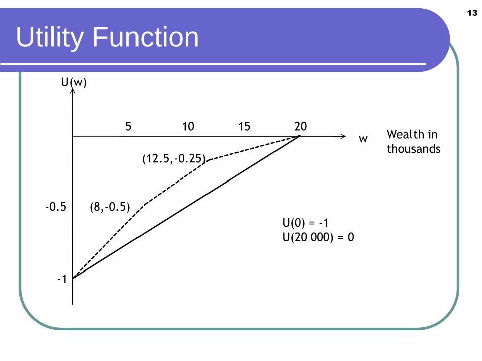
Utility Function13

w Wealth in

thousands

5 10 15 20

-1

-0.5 (8,-0.5)

(12.5,-0.25)

U(0) = -1

U(20 000) = 0

U(w)

Utility Function14

Suppose you face a loss of 20,000 with probability 0.5, and will

remain at your current level of wealth with probability 0.5. What is

the maximum amount G you would be willing to pay for complete

insurance protection against this random loss?

u(20,000 – G) = 0.5 u(20,000) + 0.5 u(0)

= (0.5)(0) + (0.5)(-1) = - 0.5?

Suppose the decision maker’s answer is G = 12,000. Therefore:

u(20,000-12,000) = u(8,000) = -0.5

(8, -0.5)

The decision maker is willing to pay an amount for insurance that is

greater than (0.5)(0) + (0.5)(20,000) = 10,000.

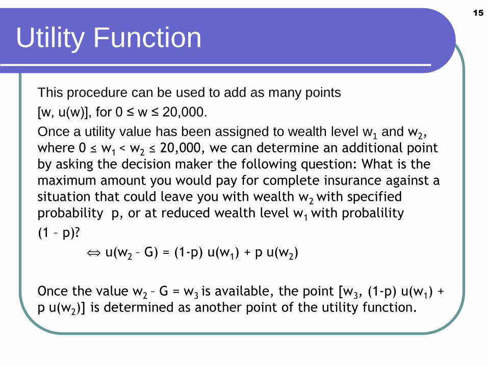
Utility Function15

This procedure can be used to add as many points

[w, u(w)], for 0 ≤ w ≤ 20,000.

Once a utility value has been assigned to wealth level w1 and w2,

where 0 ≤ w1 < w2 ≤ 20,000, we can determine an additional point

by asking the decision maker the following question: What is the

maximum amount you would pay for complete insurance against a

situation that could leave you with wealth w2 with specified

probability p, or at reduced wealth level w1 with probalility

(1 – p)?

u(w2 – G) = (1-p) u(w1) + p u(w2)

Once the value w2 – G = w3 is available, the point [w3, (1-p) u(w1) +

p u(w2)] is determined as another point of the utility function.

Utility Function16

After a decision maker has determined his utility of wealth

function by method outlined, the function can be used to compare

two random economic prospects. The prospects are denoted by

the random variables X and Y.

• If the decision maker has wealth w, and must compare the

random prospects X and Y, the decision maker selects X if

E[u(w+X)] > E[u(w+Y)]

• The decision maker is indifferent between X and Y if

E[u(w+X)] = E[u(w+Y)]

1.3 Insurance and Utility17

• Suppose a decision maker owns a property that may be

damaged or destroyed in the next accounting period.

The amount of the loss, which may be 0, is a random

variable denoted by X. We assume that the distribution

of X is known. Then E[X], the expected loss in the next

period, may be interpreted as the long-term average

loss if the experiment of exposing the property to

damage may be observed under identical conditions a

great many times.

1.3 Insurance and Utility18

• Suppose that an insurance organization (insurer) was

established to help reduce the financial consequences

of the damage or destruction of property. The insurer

would issue contracts (policies) that would promise to

pay the owner of a property a defined amount equal to

or less than the financial loss if the property were

damaged or destroyed during the period of the policy.

The contingent payment linked to the amount of the

loss is called a claim payment. In return for the

promise contained in the policy, the owner of the

property (insured) pays a consideration (premium).

Contingent = kesatuan

1.3 Insurance and Utility19

• The insurer would set its basic price for full insurance

coverage as the expected loss, E[X] = . In this context

is called the pure or net premium for the 1-period

insurance policy. To provide for expences, taxes, and

profit and for some security against adverse loss

experience, the insurance system would decide to set

the premium for the policy by loading, adding to, the

pure premium. The loaded premium, denoted by H,

might be given by

H = (1 + a) + c, a > 0, c > 0.

1.3 Insurance and Utility20

• Application: The property owner has a utility function

u(w) where wealth w is measured in monetary terms.

The owner faces a possible loss due to random events

that may damage the property. The distribution of the

random loss is assumed to be known.

u(w – G) = E[u(w - X)]

• Left-hand side: utility of paying G for complete financial

protection.

• Right-hand side: expected utility of not buying insurance

when the owner’s current wealth is w.

1.3 Insurance and Utility21

• If the owner has an increasing linear utility function, that

is u(w) = bw + d, with b > 0, the owner will be adopting

the expected value principle. In this case the owners

prefers, or indifferent to the insurance when

u(w-G) ≥ E[u(w-X)]

b (w-G) + d ≥ E[b(w-X) + d]

b (w-G) + d ≥ b(w-) + d

G ≤

The premium payments that will make the owner

prefer, or indifferent to, complete insurance are

less than or equal to the expected loss.

Utility Function22

1. u’(w) > 0 u is an increasing function.

2. U’’(w) < 0 u is a strictly concave downward

function.

Example:

An exponensial utility function:

Therefore, u(w) may serve as the utility function of a risk-

averse individual.

( ) , 0.wu w e

20; 0w wu w e u w e

Utility Function23

[ ]

[ ]

[ ]

log

w G w X

G X

X

X

u w G E u w X

e E e

e E e M

MG

Verification for the insured:

Utility Function24

Verification for the insurer:

[ ]

[ ]

log

w H Xw

w Hw

X

X

u w E u w H X

e E e

e e M

MH

Example 1.3.125

A decision maker’s utility function is given by

The decision maker has two random economic prospects

(gains) available. The outcome of the first, denoted by X,

has normal ( = 5, 2 = 2). The second prospect,

denoted by Y, is distributed as normal ( = 6, 2 = 2.5).

Which prospect will be prefered?

5( ) wu w e

2

2

5 [ 5(5) (5 )(2)/2]

5 [ 5(6) (5 )(2.5)/2] 1.25

1.25

[ ( )] [ ] ( 5) 1.

[ ( )] [ ] ( 5) .

Therefore, [ ( )] 1 [ ( )] .

X

X

Y

Y

E u X E e M e

E u Y E e M e e

E u X E u Y e

Example 1.3.226

A decision maker’s utility function is given by

The decision maker has wealth of w = 10 and faces a

random loss X with a uniform distribution on (0, 10).

What is the maximum amount this decision maker will

pay for complete insurance against the random loss?

( )u w w

10

0

103/2

0

( ) [ ( )]

1[ 10 ] 10

10

2(10 ) 210 5.5556

3(10) 3

u w G E u w X

w G E X X dx

xG

Example 1.3.327

A decision maker’s utility function is given by

The decision maker will retain wealth of amount w with

probability p and suffer a financial loss of amount c with

probability 1- p. For the values of w, c, and p exhibited in

the table below, find the maximum insurance premium

that the decision maker will pay for complete insurance.

Assume c ≤ w < 50.

2( ) 0.01 , 50u w w w w

Wealth w Loss c Probability p Insurance

Premium G

10 10 0.5 ?

20 10 0.5 ?

Example 1.3.328

2

2 2

( ) [ ( )]

( ) ( ) (1 ) ( )

( ) 0.01

0.01 (1 ) [( ) 0.01( ) ]

u w G E u w X

u w G pu w p u w c

w G w G

p w w p w c w c

For given values of w, p, and c this expression becomes

a quadratic equation. G = 5.28 and G = 5.37.