Embed Size (px)
Citation preview
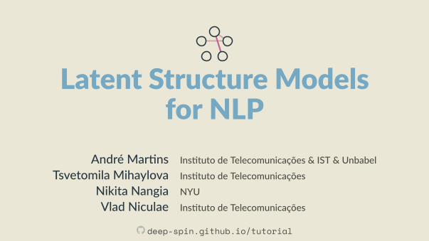
Latent Structure Modelsfor NLP
André Mar ns Ins tuto de Telecomunicações & IST & UnbabelTsvetomila Mihaylova Ins tuto de Telecomunicações
Nikita Nangia NYUVlad Niculae Ins tuto de Telecomunicações
deep-spin.github.io/tutorial

I. Introduc on
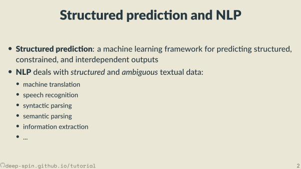
Structured predic on and NLP
• Structured predic on: a machine learning framework for predic ng structured,constrained, and interdependent outputs• NLP deals with structured and ambiguous textual data:• machine transla on• speech recogni on• syntac c parsing• seman c parsing• informa on extrac on• ...
deep-spin.github.io/tutorial 2
Examples of structure in NLP
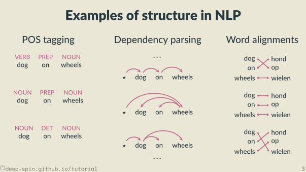
POS taggingVERB PREP NOUNdog on wheels
NOUN PREP NOUNdog on wheels
NOUN DET NOUNdog on wheels
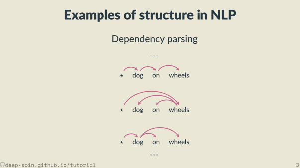
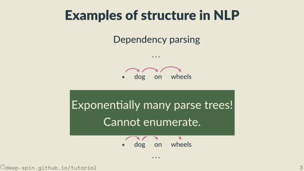
Dependency parsing· · ·
⋆ dog on wheels
⋆ dog on wheels
⋆ dog on wheels
· · ·
Word alignments
dogon
wheels
hondopwielen
dogon
wheels
hondopwielen
dogon
wheels
hondopwielen
Exponen ally many parse trees!Cannot enumerate.
deep-spin.github.io/tutorial 3
Examples of structure in NLP
POS taggingVERB PREP NOUNdog on wheels
NOUN PREP NOUNdog on wheels
NOUN DET NOUNdog on wheels
Dependency parsing· · ·
⋆ dog on wheels
⋆ dog on wheels
⋆ dog on wheels
· · ·
Word alignments
dogon
wheels
hondopwielen
dogon
wheels
hondopwielen
dogon
wheels
hondopwielen
Exponen ally many parse trees!Cannot enumerate.
deep-spin.github.io/tutorial 3
Examples of structure in NLPPOS tagging
VERB PREP NOUNdog on wheels
NOUN PREP NOUNdog on wheels
NOUN DET NOUNdog on wheels
Dependency parsing· · ·
⋆ dog on wheels
⋆ dog on wheels
⋆ dog on wheels
· · ·
Word alignments
dogon
wheels
hondopwielen
dogon
wheels
hondopwielen
dogon
wheels
hondopwielen
Exponen ally many parse trees!Cannot enumerate.
deep-spin.github.io/tutorial 3

NLP 5 years ago:Structured predic on and pipelines
NLP 5 years ago:Structured predic on and pipelines
• Big pipeline systems, connec ng di erent structured predictors, trainedseparately• Advantages: fast and simple to train, can rearrange pieces
• Disadvantage: linguis c annota ons required for each component• Bigger disadvantage: error propagates through the pipeline
deep-spin.github.io/tutorial 5
NLP 5 years ago:Structured predic on and pipelines
• Big pipeline systems, connec ng di erent structured predictors, trainedseparately• Advantages: fast and simple to train, can rearrange pieces• Disadvantage: linguis c annota ons required for each component
• Bigger disadvantage: error propagates through the pipeline
deep-spin.github.io/tutorial 5
NLP 5 years ago:Structured predic on and pipelines
• Big pipeline systems, connec ng di erent structured predictors, trainedseparately• Advantages: fast and simple to train, can rearrange pieces• Disadvantage: linguis c annota ons required for each component• Bigger disadvantage: error propagates through the pipeline
deep-spin.github.io/tutorial 5
NLP today:End-to-end training
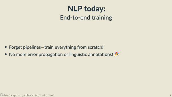
NLP today:End-to-end training
• Forget pipelines—train everything from scratch!• No more error propaga on or linguis c annota ons!
• Treat everything as latent!
deep-spin.github.io/tutorial 7
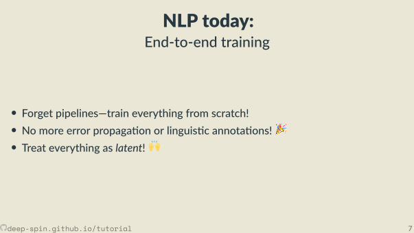
NLP today:End-to-end training
• Forget pipelines—train everything from scratch!• No more error propaga on or linguis c annota ons!• Treat everything as latent!
deep-spin.github.io/tutorial 7
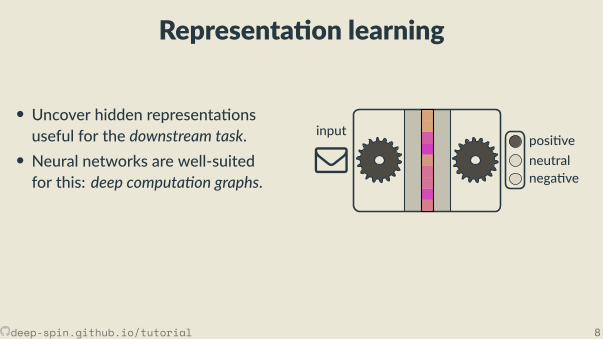
Representa on learning
• Uncover hidden representa onsuseful for the downstream task.• Neural networks are well-suitedfor this: deep computa on graphs.
• Neural representa ons areunstructured, inscrutable.Language data has underlyingstructure!
posi veneutralnega ve
input
deep-spin.github.io/tutorial 8
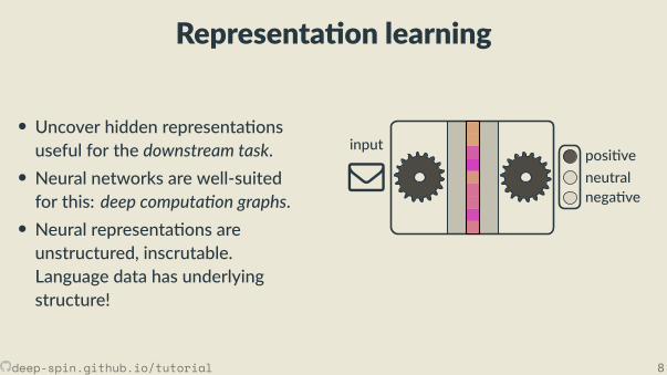
Representa on learning
• Uncover hidden representa onsuseful for the downstream task.• Neural networks are well-suitedfor this: deep computa on graphs.• Neural representa ons areunstructured, inscrutable.Language data has underlyingstructure!
posi veneutralnega ve
input
deep-spin.github.io/tutorial 8
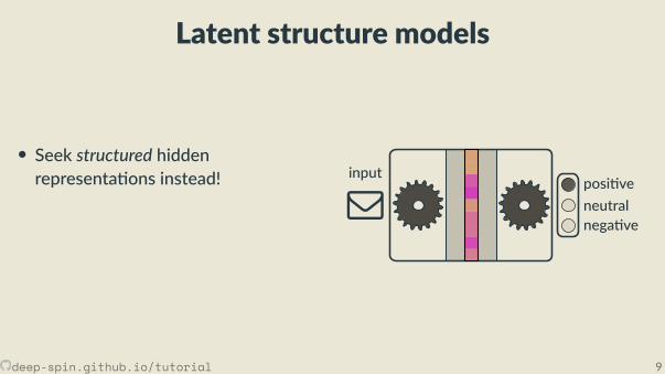
Latent structure models
• Seek structured hiddenrepresenta ons instead! posi ve
neutralnega ve
input
deep-spin.github.io/tutorial 9
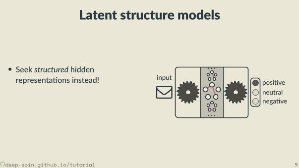
Latent structure models
• Seek structured hiddenrepresenta ons instead! posi ve
neutralnega ve
input· · ·
· · ·
deep-spin.github.io/tutorial 9
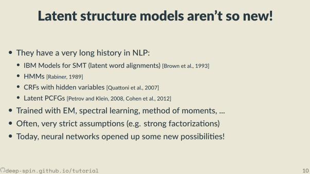
Latent structure models aren’t so new!
• They have a very long history in NLP:• IBM Models for SMT (latent word alignments) [Brown et al., 1993]• HMMs [Rabiner, 1989]• CRFs with hidden variables [Qua oni et al., 2007]• Latent PCFGs [Petrov and Klein, 2008, Cohen et al., 2012]• Trained with EM, spectral learning, method of moments, ...• O en, very strict assump ons (e.g. strong factoriza ons)• Today, neural networks opened up some new possibili es!
deep-spin.github.io/tutorial 10
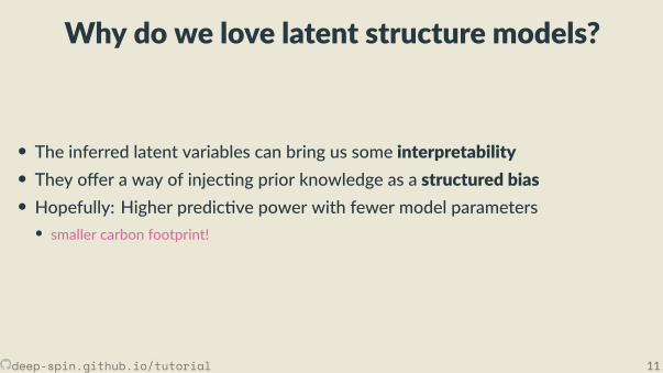
Why do we love latent structure models?
• The inferred latent variables can bring us some interpretability• They o er a way of injec ng prior knowledge as a structured bias• Hopefully: Higher predic ve power with fewer model parameters
• smaller carbon footprint!
deep-spin.github.io/tutorial 11
Why do we love latent structure models?
• The inferred latent variables can bring us some interpretability• They o er a way of injec ng prior knowledge as a structured bias• Hopefully: Higher predic ve power with fewer model parameters• smaller carbon footprint!
deep-spin.github.io/tutorial 11
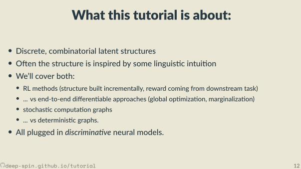
What this tutorial is about:
• Discrete, combinatorial latent structures• O en the structure is inspired by some linguis c intui on• We’ll cover both:• RL methods (structure built incrementally, reward coming from downstream task)• ... vs end-to-end di eren able approaches (global op miza on, marginaliza on)• stochas c computa on graphs• ... vs determinis c graphs.• All plugged in discrimina ve neural models.
deep-spin.github.io/tutorial 12
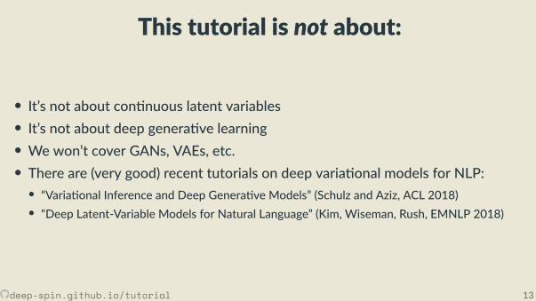
This tutorial is not about:
• It’s not about con nuous latent variables• It’s not about deep genera ve learning• We won’t cover GANs, VAEs, etc.• There are (very good) recent tutorials on deep varia onal models for NLP:• “Varia onal Inference and Deep Genera ve Models” (Schulz and Aziz, ACL 2018)• “Deep Latent-Variable Models for Natural Language” (Kim, Wiseman, Rush, EMNLP 2018)
deep-spin.github.io/tutorial 13

Background
Unstructured vs structured
• To be er explain the math, we’ll o en backtrack to unstructuredmodels (wherethe latent variable is a categorical) before jumping to the structured ones
deep-spin.github.io/tutorial 14
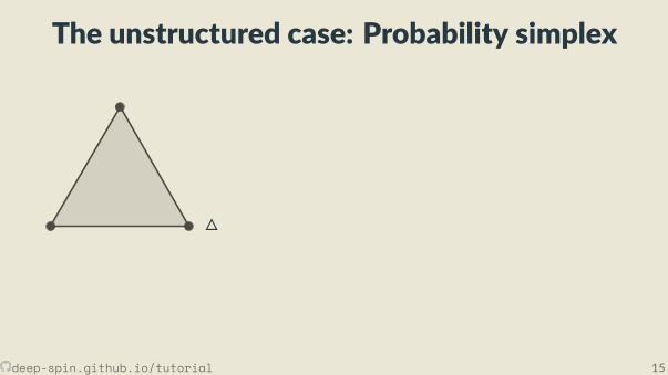
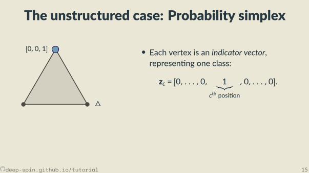
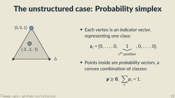
The unstructured case: Probability simplex
[0,0,1]
[.3, .2, .5]
• Each vertex is an indicator vector,represen ng one class:
zc = [0, . . . ,0, 1︸︷︷︸cth posi on
,0, . . . ,0].
• Points inside are probability vectors, aconvex combina on of classes:
p ≥ 0,∑cpc = 1.
deep-spin.github.io/tutorial 15
The unstructured case: Probability simplex
[0,0,1]
[.3, .2, .5]
• Each vertex is an indicator vector,represen ng one class:
zc = [0, . . . ,0, 1︸︷︷︸cth posi on
,0, . . . ,0].
• Points inside are probability vectors, aconvex combina on of classes:
p ≥ 0,∑cpc = 1.
deep-spin.github.io/tutorial 15
The unstructured case: Probability simplex
[0,0,1]
[.3, .2, .5]
• Each vertex is an indicator vector,represen ng one class:
zc = [0, . . . ,0, 1︸︷︷︸cth posi on
,0, . . . ,0].
• Points inside are probability vectors, aconvex combina on of classes:
p ≥ 0,∑cpc = 1.
deep-spin.github.io/tutorial 15
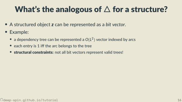
What’s the analogous of for a structure?• A structured object z can be represented as a bit vector.
• Example:
• a dependency tree can be represented a O(L2) vector indexed by arcs• each entry is 1 i the arc belongs to the tree• structural constraints: not all bit vectors represent valid trees!
z1 = [1,0,0,0,1,0,0,0,1]
⋆ dog on wheels
z2 = [0,0,1,0,0,1,1,0,0]
⋆ dog on wheels
z3 = [1,0,0,0,1,0,0,1,0]
⋆ dog on wheels
deep-spin.github.io/tutorial 16
What’s the analogous of for a structure?• A structured object z can be represented as a bit vector.• Example:• a dependency tree can be represented a O(L2) vector indexed by arcs• each entry is 1 i the arc belongs to the tree• structural constraints: not all bit vectors represent valid trees!
z1 = [1,0,0,0,1,0,0,0,1]
⋆ dog on wheels
z2 = [0,0,1,0,0,1,1,0,0]
⋆ dog on wheels
z3 = [1,0,0,0,1,0,0,1,0]
⋆ dog on wheels
deep-spin.github.io/tutorial 16

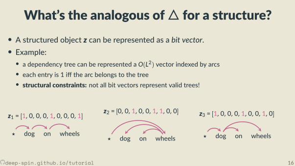
The structured case: Marginal polytope[Wainwright and Jordan, 2008]
• Each vertex corresponds to one such bit vector z• Points inside correspond to marginal distribu ons:convex combina ons of structured objects
μ = p1z1 + . . . + pNzN︸ ︷︷ ︸exponen ally many terms
, p ∈ ∆.
p1 = 0.2, z1 = [1,0,0,0,1,0,0,0,1]p2 = 0.7, z2 = [0,0,1,0,0,1,1,0,0]p3 = 0.1, z3 = [1,0,0,0,1,0,0,1,0]
⇒ μ=[.3,0, .7,0, .3, .7, .7, .1, .2].
M
deep-spin.github.io/tutorial 17
The structured case: Marginal polytope[Wainwright and Jordan, 2008]
• Each vertex corresponds to one such bit vector z
• Points inside correspond to marginal distribu ons:convex combina ons of structured objects
μ = p1z1 + . . . + pNzN︸ ︷︷ ︸exponen ally many terms
, p ∈ ∆.
p1 = 0.2, z1 = [1,0,0,0,1,0,0,0,1]p2 = 0.7, z2 = [0,0,1,0,0,1,1,0,0]p3 = 0.1, z3 = [1,0,0,0,1,0,0,1,0]
⇒ μ=[.3,0, .7,0, .3, .7, .7, .1, .2].
M
deep-spin.github.io/tutorial 17

The structured case: Marginal polytope[Wainwright and Jordan, 2008]
• Each vertex corresponds to one such bit vector z• Points inside correspond to marginal distribu ons:convex combina ons of structured objects
μ = p1z1 + . . . + pNzN︸ ︷︷ ︸exponen ally many terms
, p ∈ ∆.
p1 = 0.2, z1 = [1,0,0,0,1,0,0,0,1]p2 = 0.7, z2 = [0,0,1,0,0,1,1,0,0]p3 = 0.1, z3 = [1,0,0,0,1,0,0,1,0]
⇒ μ=[.3,0, .7,0, .3, .7, .7, .1, .2].
M
deep-spin.github.io/tutorial 17
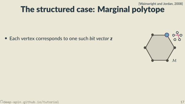
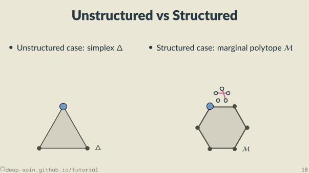
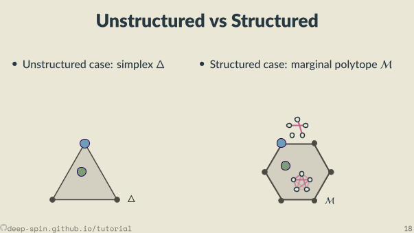
Unstructured vs Structured
• Unstructured case: simplex∆
• Structured case: marginal polytopeM
M
deep-spin.github.io/tutorial 18
Unstructured vs Structured
• Unstructured case: simplex∆
• Structured case: marginal polytopeM
M
deep-spin.github.io/tutorial 18
Unstructured vs Structured
• Unstructured case: simplex∆
• Structured case: marginal polytopeM
M
deep-spin.github.io/tutorial 18
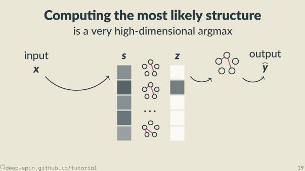
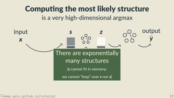
Compu ng the most likely structureis a very high-dimensional argmax
· · ·
s zinputx
outputby
There are exponen allymany structures(s cannot t in memory;
we cannot “loop” over s nor z)
deep-spin.github.io/tutorial 19
Compu ng the most likely structureis a very high-dimensional argmax
· · ·
s zinputx
outputbyThere are exponen ally
many structures(s cannot t in memory;
we cannot “loop” over s nor z)
deep-spin.github.io/tutorial 19
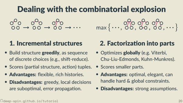
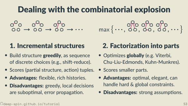
Dealing with the combinatorial explosion
→ → → · · ·1. Incremental structures• Build structure greedily, as sequenceof discrete choices (e.g., shi -reduce).• Scores (par al structure, ac on) tuples.• Advantages: exible, rich histories.• Disadvantages: greedy, local decisionsare subop mal, error propaga on.
max · · · , , , , · · ·
2. Factoriza on into parts• Op mizes globally (e.g. Viterbi,Chu-Liu-Edmonds, Kuhn-Munkres).• Scores smaller parts.• Advantages: op mal, elegant, canhandle hard & global constraints.• Disadvantages: strong assump ons.
deep-spin.github.io/tutorial 20
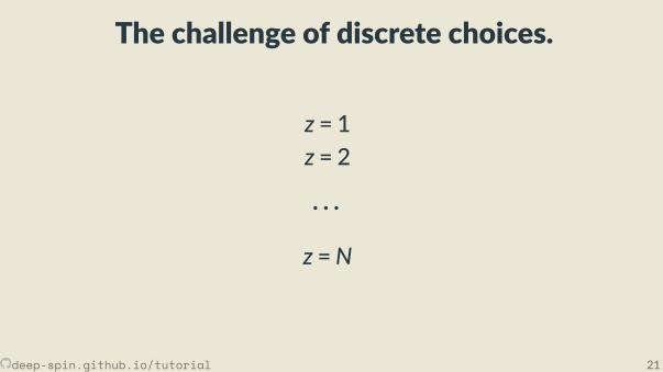
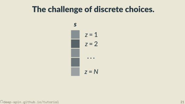
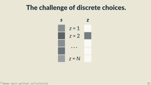
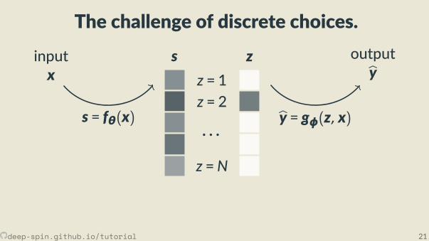
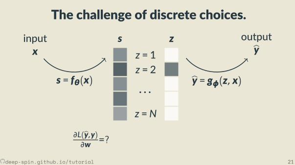
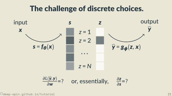
The challenge of discrete choices.
z = 1z = 2
· · ·z =N
s zinputx
outputbys = fθ(x) by = gφ(z, x)
∂L(by,y)∂w =? or, essen ally, ∂z
∂s=?
deep-spin.github.io/tutorial 21
The challenge of discrete choices.
z = 1z = 2
· · ·z =N
s
zinputx
outputbys = fθ(x) by = gφ(z, x)
∂L(by,y)∂w =? or, essen ally, ∂z
∂s=?
deep-spin.github.io/tutorial 21
The challenge of discrete choices.
z = 1z = 2
· · ·z =N
s z
inputx
outputbys = fθ(x) by = gφ(z, x)
∂L(by,y)∂w =? or, essen ally, ∂z
∂s=?
deep-spin.github.io/tutorial 21
The challenge of discrete choices.
z = 1z = 2
· · ·z =N
s zinputx
outputbys = fθ(x) by = gφ(z, x)
∂L(by,y)∂w =? or, essen ally, ∂z
∂s=?
deep-spin.github.io/tutorial 21
The challenge of discrete choices.
z = 1z = 2
· · ·z =N
s zinputx
outputbys = fθ(x) by = gφ(z, x)
∂L(by,y)∂w =?
or, essen ally, ∂z∂s=?
deep-spin.github.io/tutorial 21
The challenge of discrete choices.
z = 1z = 2
· · ·z =N
s zinputx
outputbys = fθ(x) by = gφ(z, x)
∂L(by,y)∂w =? or, essen ally, ∂z
∂s=?
deep-spin.github.io/tutorial 21
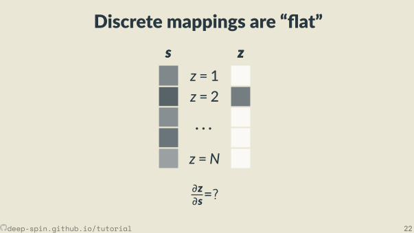
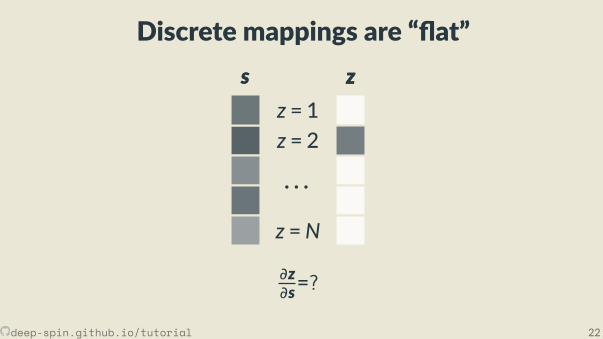
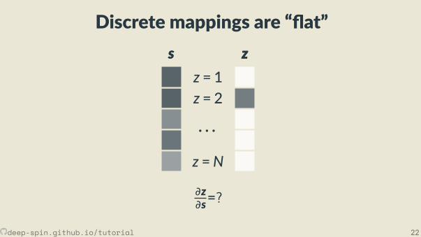
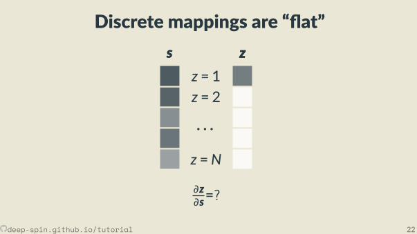
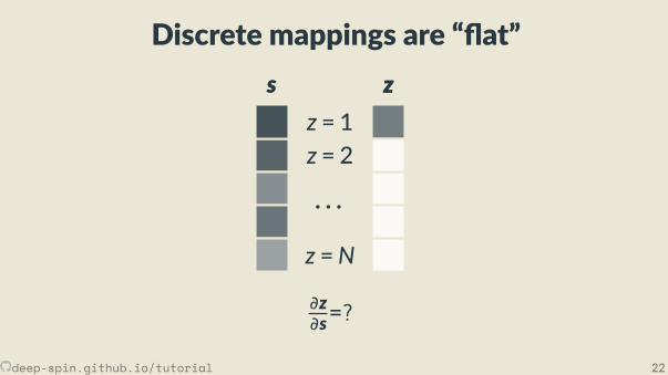
Discrete mappings are “ at”s
z = 1z = 2
· · ·z =N
s zz
∂z∂s=?
deep-spin.github.io/tutorial 22

Discrete mappings are “ at”s
z = 1z = 2
· · ·z =N
s zz
∂z∂s=?
deep-spin.github.io/tutorial 22
Discrete mappings are “ at”s
z = 1z = 2
· · ·z =N
s zz
∂z∂s=?
deep-spin.github.io/tutorial 22

Discrete mappings are “ at”s
z = 1z = 2
· · ·z =N
s zz
∂z∂s=?
deep-spin.github.io/tutorial 22
Discrete mappings are “ at”s
z = 1z = 2
· · ·z =N
s zz
∂z∂s=?
deep-spin.github.io/tutorial 22
Discrete mappings are “ at”s
z = 1z = 2
· · ·z =N
s zz
∂z∂s=?
deep-spin.github.io/tutorial 22
Discrete mappings are “ at”s
z = 1z = 2
· · ·z =N
s zz
∂z∂s=?
deep-spin.github.io/tutorial 22

Discrete mappings are “ at”s
z = 1z = 2
· · ·z =N
s zz
∂z∂s=?
deep-spin.github.io/tutorial 22
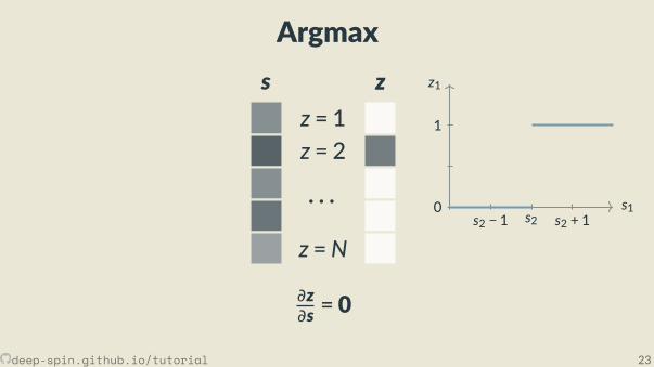
Argmax
z = 1z = 2
· · ·z =N
s z
∂z∂s = 0
z1
s10
1
s2 − 1 s2 s2 + 1
deep-spin.github.io/tutorial 23
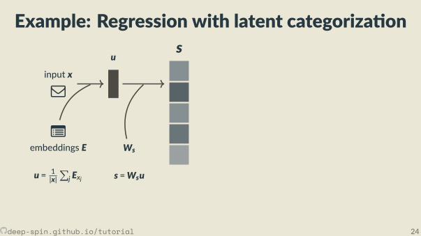
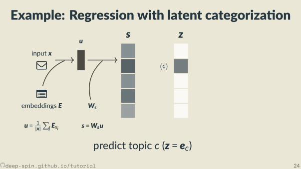
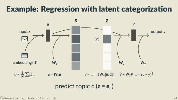
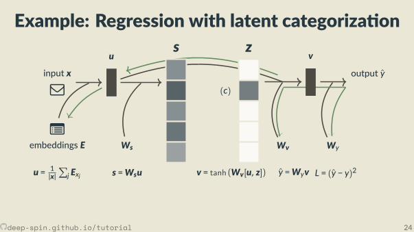
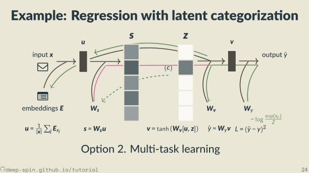
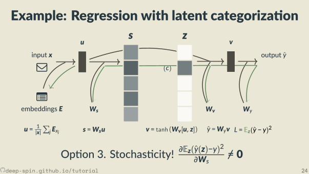
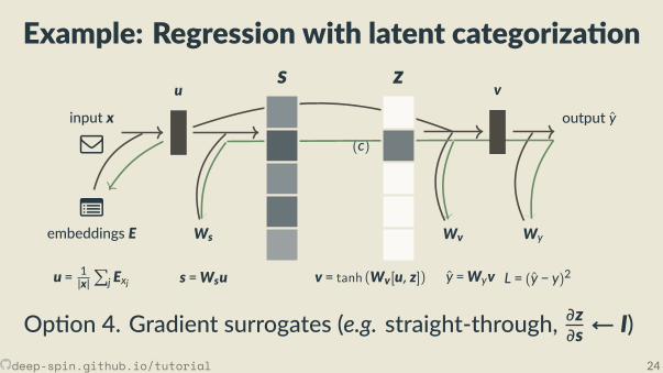
Example: Regression with latent categoriza on
(c)
s
zp
input x
u
embeddings E Ws
u = 1|x|∑
j Exj s =Wsu
output y
v
Wv Wy
v = tanh (Wv[u, z]) y =Wyv L = (y − y)2− log exp(sc)
Z
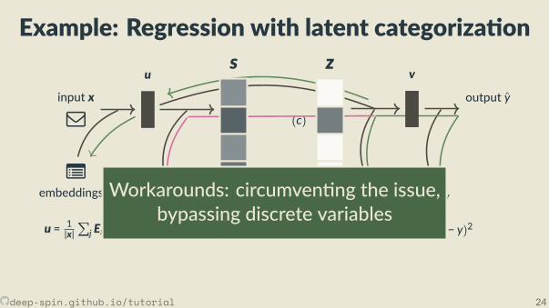
Workarounds: circumven ng the issue,bypassing discrete variablesTackling discreteness end-to-end
deep-spin.github.io/tutorial 24
Example: Regression with latent categoriza on
(c)
s z
p
input x
u
embeddings E Ws
u = 1|x|∑
j Exj s =Wsu
output y
v
Wv Wy
v = tanh (Wv[u, z]) y =Wyv L = (y − y)2− log exp(sc)
Z
predict topic c (z = ec)
Workarounds: circumven ng the issue,bypassing discrete variablesTackling discreteness end-to-end
deep-spin.github.io/tutorial 24
Example: Regression with latent categoriza on
(c)
s z
p
input x
u
embeddings E Ws
u = 1|x|∑
j Exj s =Wsu
output y
v
Wv Wy
v = tanh (Wv[u, z]) y =Wyv L = (y − y)2
− log exp(sc)Z
Workarounds: circumven ng the issue,bypassing discrete variablesTackling discreteness end-to-end
deep-spin.github.io/tutorial 24
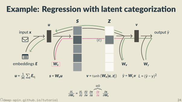
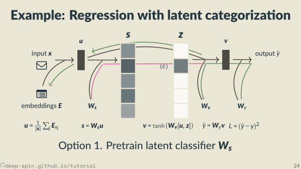
Example: Regression with latent categoriza on
(c)
s z
p
input x
u
embeddings E Ws
u = 1|x|∑
j Exj s =Wsu
output y
v
Wv Wy
v = tanh (Wv[u, z]) y =Wyv L = (y − y)2
− log exp(sc)Z
∂L∂Ws
= ∂L∂y
∂y∂v
∂v∂z
≡0︷︸︸︷∂z∂s
∂s∂Ws
Workarounds: circumven ng the issue,bypassing discrete variablesTackling discreteness end-to-end
deep-spin.github.io/tutorial 24
Example: Regression with latent categoriza on
(c)
s z
p
input x
u
embeddings E Ws
u = 1|x|∑
j Exj s =Wsu
output y
v
Wv Wy
v = tanh (Wv[u, z]) y =Wyv L = (y − y)2
− log exp(sc)Z
Workarounds: circumven ng the issue,bypassing discrete variables
Tackling discreteness end-to-end
deep-spin.github.io/tutorial 24
Example: Regression with latent categoriza on
(c)
s z
p
input x
u
embeddings E Ws
u = 1|x|∑
j Exj s =Wsu
output y
v
Wv Wy
v = tanh (Wv[u, z]) y =Wyv L = (y − y)2
− log exp(sc)Z
Op on 1. Pretrain latent classi erWs
Workarounds: circumven ng the issue,bypassing discrete variablesTackling discreteness end-to-end
deep-spin.github.io/tutorial 24
Example: Regression with latent categoriza on
(c)
s z
p
input x
u
embeddings E Ws
u = 1|x|∑
j Exj s =Wsu
output y
v
Wv Wy
v = tanh (Wv[u, z]) y =Wyv L = (y − y)2− log exp(sc)
Z
Op on 2. Mul -task learning
Workarounds: circumven ng the issue,bypassing discrete variablesTackling discreteness end-to-end
deep-spin.github.io/tutorial 24
Example: Regression with latent categoriza on
(c)
s z
p
input x
u
embeddings E Ws
u = 1|x|∑
j Exj s =Wsu
output y
v
Wv Wy
v = tanh (Wv[u, z]) y =Wyv L = (y − y)2
− log exp(sc)Z
Workarounds: circumven ng the issue,bypassing discrete variables
Tackling discreteness end-to-end
deep-spin.github.io/tutorial 24
Example: Regression with latent categoriza on
(c)
s z
p
input x
u
embeddings E Ws
u = 1|x|∑
j Exj s =Wsu
output y
v
Wv Wy
v = tanh (Wv[u, z]) y =Wyv L = Ez(y − y)2
− log exp(sc)Z
Op on 3. Stochas city! ∂Ez(y(z)−y)2
∂Ws=/ 0
Workarounds: circumven ng the issue,bypassing discrete variablesTackling discreteness end-to-end
deep-spin.github.io/tutorial 24
Example: Regression with latent categoriza on
(c)
s z
p
input x
u
embeddings E Ws
u = 1|x|∑
j Exj s =Wsu
output y
v
Wv Wy
v = tanh (Wv[u, z]) y =Wyv L = (y − y)2
− log exp(sc)Z
Op on 4. Gradient surrogates (e.g. straight-through, ∂z∂s ← I)
Workarounds: circumven ng the issue,bypassing discrete variablesTackling discreteness end-to-end
deep-spin.github.io/tutorial 24
Example: Regression with latent categoriza on
(c)
s
z
p
input x
u
embeddings E Ws
u = 1|x|∑
j Exj s =Wsu
output y
v
Wv Wy
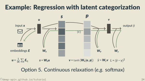
v = tanh (Wv[u,p]) y =Wyv L = (y − y)2
− log exp(sc)Z
Op on 5. Con nuous relaxa on (e.g. so max)
Workarounds: circumven ng the issue,bypassing discrete variablesTackling discreteness end-to-end
deep-spin.github.io/tutorial 24
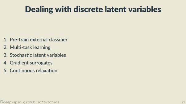
Dealing with discrete latent variables
1. Pre-train external classi er2. Mul -task learning3. Stochas c latent variables
(Part 2)
4. Gradient surrogates
(Part 3)
5. Con nuous relaxa on
(Part 4)
deep-spin.github.io/tutorial 25
Dealing with discrete latent variables
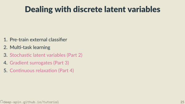
1. Pre-train external classi er2. Mul -task learning3. Stochas c latent variables (Part 2)4. Gradient surrogates (Part 3)5. Con nuous relaxa on (Part 4)
deep-spin.github.io/tutorial 25
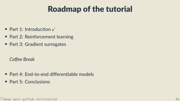
Roadmap of the tutorial
• Part 1: Introduc on • Part 2: Reinforcement learning• Part 3: Gradient surrogates
Co ee Break
• Part 4: End-to-end di eren able models• Part 5: Conclusions
deep-spin.github.io/tutorial 26
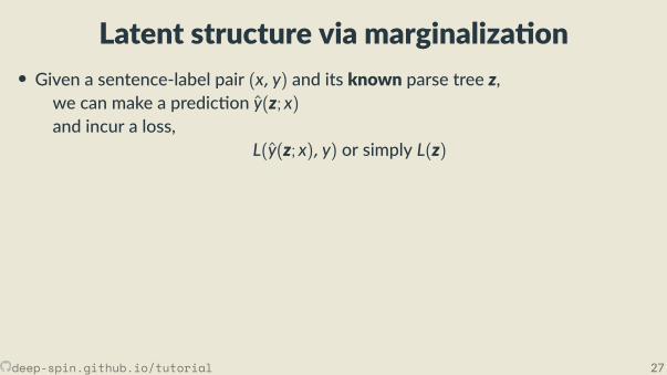
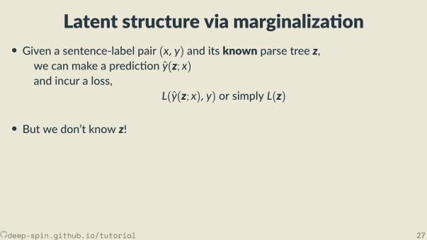
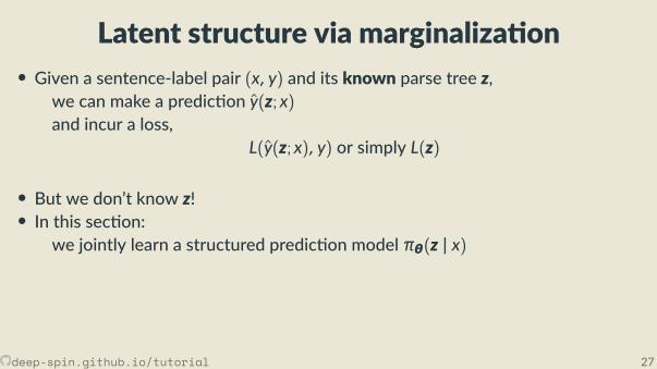
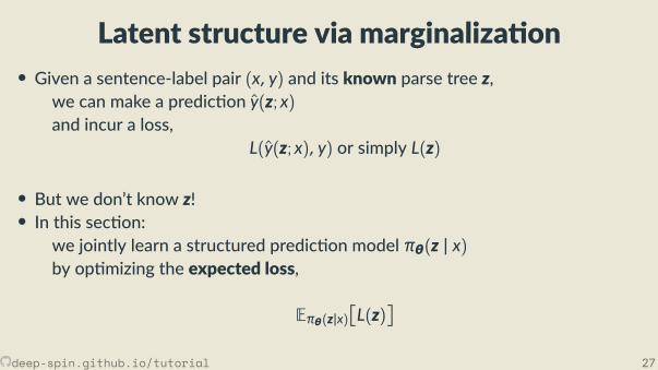
II. ReinforcementLearning Methods
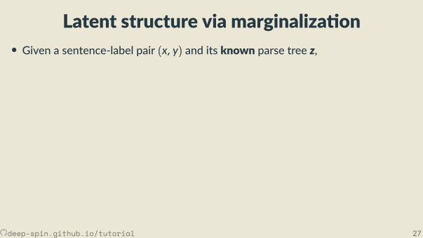
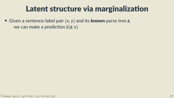
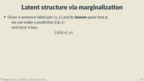
Latent structure via marginaliza on• Given a sentence-label pair (x, y) and its known parse tree z,
we can make a predic on y(z; x)and incur a loss,
L(y(z; x), y)
or simply L(z)
• But we don’t know z!• In this sec on:
we jointly learn a structured predic on model πθ(z | x)
by op mizing the expected loss,
Eπθ(z|x)L(z)
deep-spin.github.io/tutorial 27
Latent structure via marginaliza on• Given a sentence-label pair (x, y) and its known parse tree z,
we can make a predic on y(z; x)
and incur a loss,L(y(z; x), y)
or simply L(z)
• But we don’t know z!• In this sec on:
we jointly learn a structured predic on model πθ(z | x)
by op mizing the expected loss,
Eπθ(z|x)L(z)
deep-spin.github.io/tutorial 27
Latent structure via marginaliza on• Given a sentence-label pair (x, y) and its known parse tree z,
we can make a predic on y(z; x)and incur a loss,
L(y(z; x), y)
or simply L(z)
• But we don’t know z!• In this sec on:
we jointly learn a structured predic on model πθ(z | x)
by op mizing the expected loss,
Eπθ(z|x)L(z)
deep-spin.github.io/tutorial 27
Latent structure via marginaliza on• Given a sentence-label pair (x, y) and its known parse tree z,
we can make a predic on y(z; x)and incur a loss,
L(y(z; x), y) or simply L(z)
• But we don’t know z!
• In this sec on:we jointly learn a structured predic on model πθ(z | x)
by op mizing the expected loss,
Eπθ(z|x)L(z)
deep-spin.github.io/tutorial 27
Latent structure via marginaliza on• Given a sentence-label pair (x, y) and its known parse tree z,
we can make a predic on y(z; x)and incur a loss,
L(y(z; x), y) or simply L(z)
• But we don’t know z!• In this sec on:
we jointly learn a structured predic on model πθ(z | x)
by op mizing the expected loss,
Eπθ(z|x)L(z)
deep-spin.github.io/tutorial 27
Latent structure via marginaliza on• Given a sentence-label pair (x, y) and its known parse tree z,
we can make a predic on y(z; x)and incur a loss,
L(y(z; x), y) or simply L(z)
• But we don’t know z!• In this sec on:
we jointly learn a structured predic on model πθ(z | x)by op mizing the expected loss,
Eπθ(z|x)L(z)
deep-spin.github.io/tutorial 27
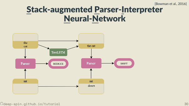
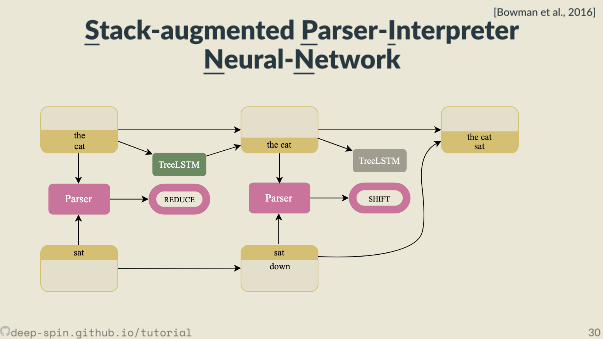
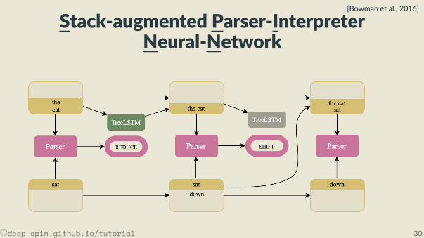
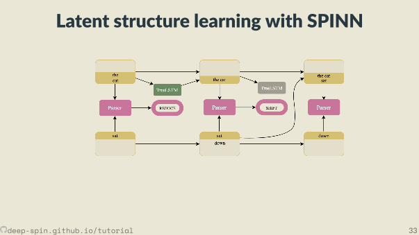
But rst, supervisedSPINN
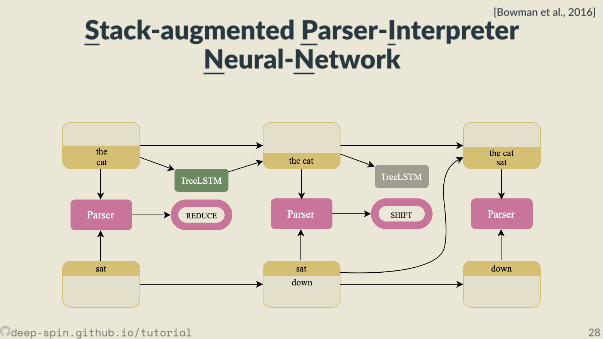
Stack-augmented Parser-InterpreterNeural-Network
[Bowman et al., 2016]
deep-spin.github.io/tutorial 28
Stack-augmented Parser-InterpreterNeural-Network
[Bowman et al., 2016]
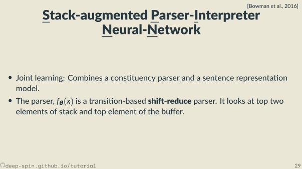
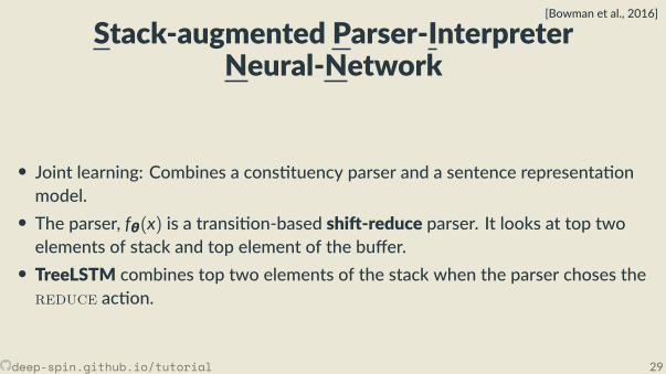
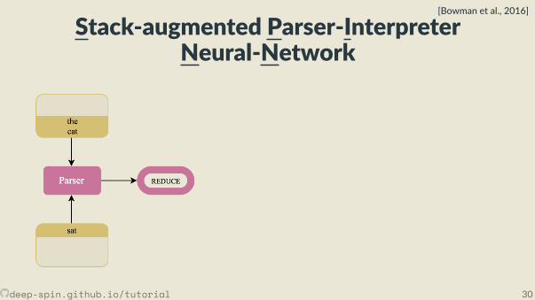
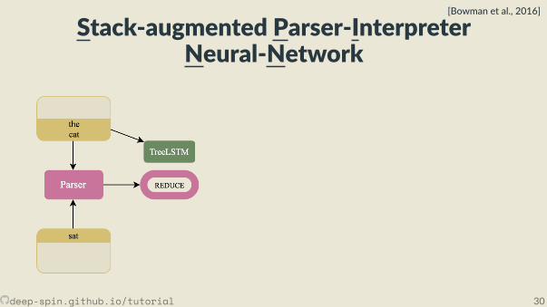
• Joint learning: Combines a cons tuency parser and a sentence representa onmodel.
• The parser, fθ(x) is a transi on-based shi -reduce parser. It looks at top twoelements of stack and top element of the bu er.• TreeLSTM combines top two elements of the stack when the parser choses the
reduce ac on.
deep-spin.github.io/tutorial 29
Stack-augmented Parser-InterpreterNeural-Network
[Bowman et al., 2016]
• Joint learning: Combines a cons tuency parser and a sentence representa onmodel.• The parser, fθ(x) is a transi on-based shi -reduce parser. It looks at top twoelements of stack and top element of the bu er.
• TreeLSTM combines top two elements of the stack when the parser choses thereduce ac on.
deep-spin.github.io/tutorial 29
Stack-augmented Parser-InterpreterNeural-Network
[Bowman et al., 2016]
• Joint learning: Combines a cons tuency parser and a sentence representa onmodel.• The parser, fθ(x) is a transi on-based shi -reduce parser. It looks at top twoelements of stack and top element of the bu er.• TreeLSTM combines top two elements of the stack when the parser choses the
reduce ac on.
deep-spin.github.io/tutorial 29
Stack-augmented Parser-InterpreterNeural-Network
[Bowman et al., 2016]
deep-spin.github.io/tutorial 30
Stack-augmented Parser-InterpreterNeural-Network
[Bowman et al., 2016]
deep-spin.github.io/tutorial 30
Stack-augmented Parser-InterpreterNeural-Network
[Bowman et al., 2016]
deep-spin.github.io/tutorial 30
Stack-augmented Parser-InterpreterNeural-Network
[Bowman et al., 2016]
deep-spin.github.io/tutorial 30
Stack-augmented Parser-InterpreterNeural-Network
[Bowman et al., 2016]
deep-spin.github.io/tutorial 30
Stack-augmented Parser-InterpreterNeural-Network
[Bowman et al., 2016]
deep-spin.github.io/tutorial 30
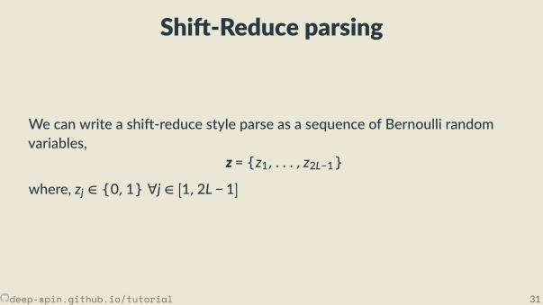
Shi -Reduce parsing
We can write a shi -reduce style parse as a sequence of Bernoulli randomvariables,
z = z1, . . . , z2L−1
where, zj ∈ 0,1 ∀j ∈ [1,2L − 1]
deep-spin.github.io/tutorial 31
Shi -Reduce parsing
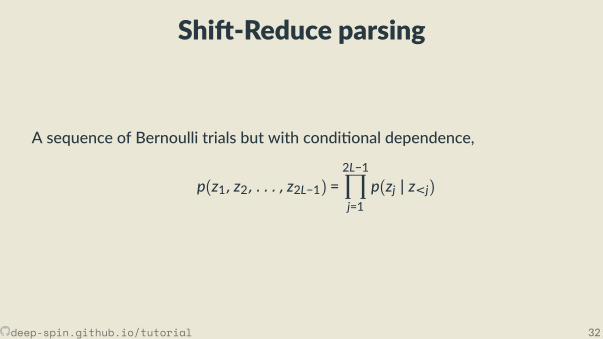
A sequence of Bernoulli trials but with condi onal dependence,
p(z1, z2, . . . , z2L−1) =2L−1∏j=1
p(zj | z<j)
deep-spin.github.io/tutorial 32
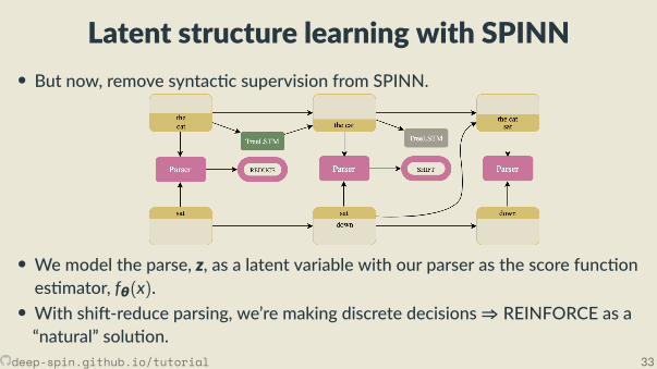
Latent structure learning with SPINN
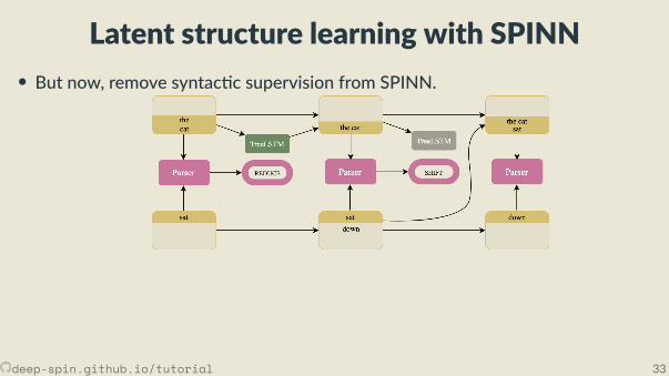
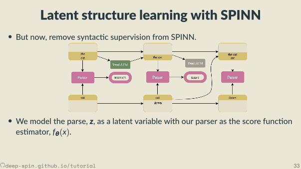
• But now, remove syntac c supervision from SPINN.
• We model the parse, z, as a latent variable with our parser as the score func ones mator, fθ(x).• With shi -reduce parsing, we’re making discrete decisions⇒ REINFORCE as a“natural” solu on.
deep-spin.github.io/tutorial 33
Latent structure learning with SPINN• But now, remove syntac c supervision from SPINN.
• We model the parse, z, as a latent variable with our parser as the score func ones mator, fθ(x).
• With shi -reduce parsing, we’re making discrete decisions⇒ REINFORCE as a“natural” solu on.
deep-spin.github.io/tutorial 33
Latent structure learning with SPINN• But now, remove syntac c supervision from SPINN.
• We model the parse, z, as a latent variable with our parser as the score func ones mator, fθ(x).• With shi -reduce parsing, we’re making discrete decisions⇒ REINFORCE as a“natural” solu on.
deep-spin.github.io/tutorial 33
Unsupervised SPINN
Unsupervised SPINN
No syntac c supervision.Only reward is from the downstream task.We only get this reward a er parsing the full sentence.
deep-spin.github.io/tutorial 34
SPINN with REINFORCE[Williams, 1992]
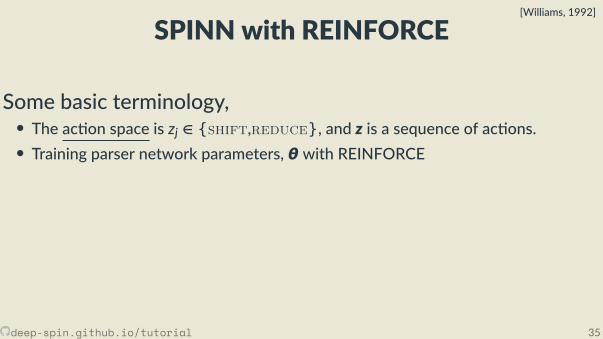
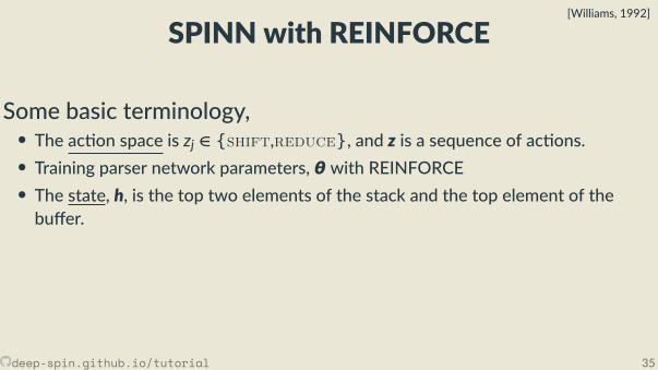
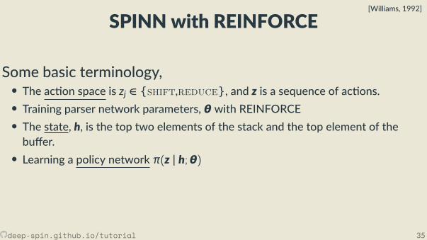
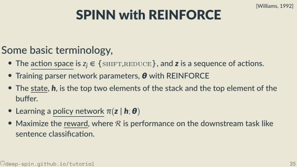
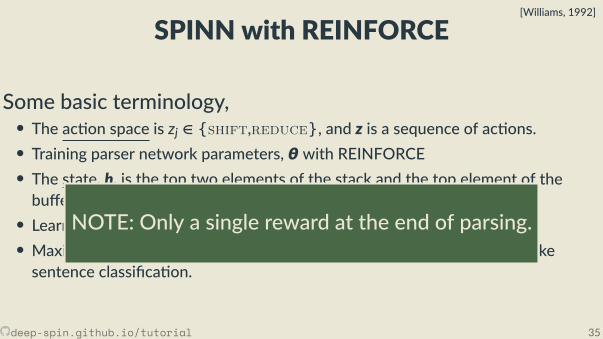
Some basic terminology,• The ac on space is zj ∈ shift,reduce, and z is a sequence of ac ons.
• Training parser network parameters, θ with REINFORCE• The state, h, is the top two elements of the stack and the top element of thebu er.• Learning a policy network π(z | h;θ)• Maximize the reward, where R is performance on the downstream task likesentence classi ca on.
NOTE: Only a single reward at the end of parsing.
deep-spin.github.io/tutorial 35
SPINN with REINFORCE[Williams, 1992]
Some basic terminology,• The ac on space is zj ∈ shift,reduce, and z is a sequence of ac ons.• Training parser network parameters, θ with REINFORCE
• The state, h, is the top two elements of the stack and the top element of thebu er.• Learning a policy network π(z | h;θ)• Maximize the reward, where R is performance on the downstream task likesentence classi ca on.
NOTE: Only a single reward at the end of parsing.
deep-spin.github.io/tutorial 35
SPINN with REINFORCE[Williams, 1992]
Some basic terminology,• The ac on space is zj ∈ shift,reduce, and z is a sequence of ac ons.• Training parser network parameters, θ with REINFORCE• The state, h, is the top two elements of the stack and the top element of thebu er.
• Learning a policy network π(z | h;θ)• Maximize the reward, where R is performance on the downstream task likesentence classi ca on.
NOTE: Only a single reward at the end of parsing.
deep-spin.github.io/tutorial 35
SPINN with REINFORCE[Williams, 1992]
Some basic terminology,• The ac on space is zj ∈ shift,reduce, and z is a sequence of ac ons.• Training parser network parameters, θ with REINFORCE• The state, h, is the top two elements of the stack and the top element of thebu er.• Learning a policy network π(z | h;θ)
• Maximize the reward, where R is performance on the downstream task likesentence classi ca on.
NOTE: Only a single reward at the end of parsing.
deep-spin.github.io/tutorial 35
SPINN with REINFORCE[Williams, 1992]
Some basic terminology,• The ac on space is zj ∈ shift,reduce, and z is a sequence of ac ons.• Training parser network parameters, θ with REINFORCE• The state, h, is the top two elements of the stack and the top element of thebu er.• Learning a policy network π(z | h;θ)• Maximize the reward, where R is performance on the downstream task likesentence classi ca on.
NOTE: Only a single reward at the end of parsing.
deep-spin.github.io/tutorial 35
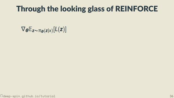
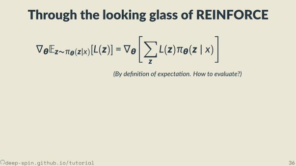
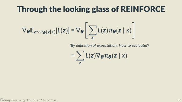
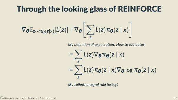
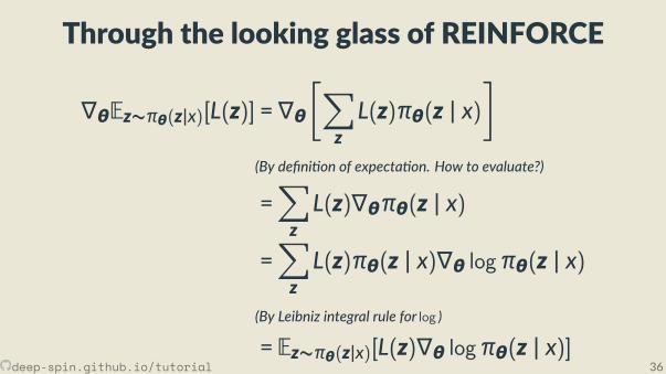
Through the looking glass of REINFORCE
∇θEz∼πθ(z|x)[L(z)]
= ∇θ∑
zL(z)πθ(z | x)
(By de ni on of expecta on. How to evaluate?)
=∑zL(z)∇θπθ(z | x)
=∑zL(z)πθ(z | x)∇θ logπθ(z | x)
(By Leibniz integral rule for log )
= Ez∼πθ(z|x)[L(z)∇θ logπθ(z | x)]
deep-spin.github.io/tutorial 36
Through the looking glass of REINFORCE
∇θEz∼πθ(z|x)[L(z)] = ∇θ∑
zL(z)πθ(z | x)
(By de ni on of expecta on. How to evaluate?)
=∑zL(z)∇θπθ(z | x)
=∑zL(z)πθ(z | x)∇θ logπθ(z | x)
(By Leibniz integral rule for log )
= Ez∼πθ(z|x)[L(z)∇θ logπθ(z | x)]
deep-spin.github.io/tutorial 36
Through the looking glass of REINFORCE
∇θEz∼πθ(z|x)[L(z)] = ∇θ∑
zL(z)πθ(z | x)
(By de ni on of expecta on. How to evaluate?)
=∑zL(z)∇θπθ(z | x)
=∑zL(z)πθ(z | x)∇θ logπθ(z | x)
(By Leibniz integral rule for log )
= Ez∼πθ(z|x)[L(z)∇θ logπθ(z | x)]
deep-spin.github.io/tutorial 36
Through the looking glass of REINFORCE
∇θEz∼πθ(z|x)[L(z)] = ∇θ∑
zL(z)πθ(z | x)
(By de ni on of expecta on. How to evaluate?)
=∑zL(z)∇θπθ(z | x)
=∑zL(z)πθ(z | x)∇θ logπθ(z | x)
(By Leibniz integral rule for log )
= Ez∼πθ(z|x)[L(z)∇θ logπθ(z | x)]
deep-spin.github.io/tutorial 36
Through the looking glass of REINFORCE
∇θEz∼πθ(z|x)[L(z)] = ∇θ∑
zL(z)πθ(z | x)
(By de ni on of expecta on. How to evaluate?)
=∑zL(z)∇θπθ(z | x)
=∑zL(z)πθ(z | x)∇θ logπθ(z | x)
(By Leibniz integral rule for log )
= Ez∼πθ(z|x)[L(z)∇θ logπθ(z | x)]deep-spin.github.io/tutorial 36
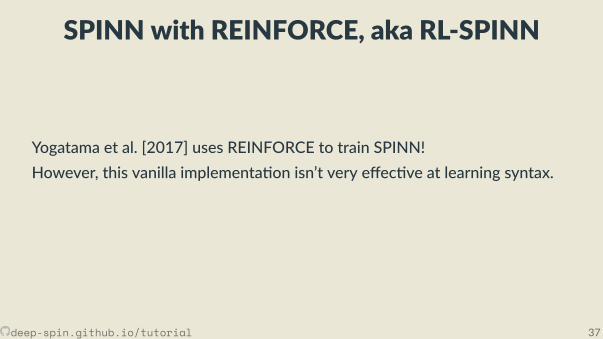
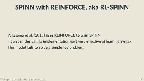
SPINN with REINFORCE, aka RL-SPINN
Yogatama et al. [2017] uses REINFORCE to train SPINN!
However, this vanilla implementa on isn’t very e ec ve at learning syntax.This model fails to solve a simple toy problem.
deep-spin.github.io/tutorial 37
SPINN with REINFORCE, aka RL-SPINN
Yogatama et al. [2017] uses REINFORCE to train SPINN!However, this vanilla implementa on isn’t very e ec ve at learning syntax.
This model fails to solve a simple toy problem.
deep-spin.github.io/tutorial 37
SPINN with REINFORCE, aka RL-SPINN
Yogatama et al. [2017] uses REINFORCE to train SPINN!However, this vanilla implementa on isn’t very e ec ve at learning syntax.This model fails to solve a simple toy problem.
deep-spin.github.io/tutorial 37
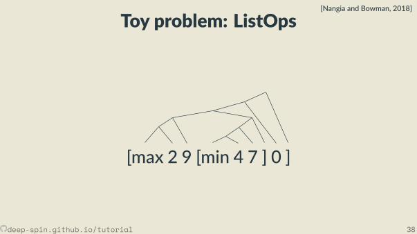
Toy problem: ListOps[Nangia and Bowman, 2018]
[max 2 9 [min 4 7 ] 0 ]
deep-spin.github.io/tutorial 38
Toy problem: ListOps[Nangia and Bowman, 2018]
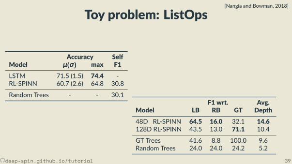
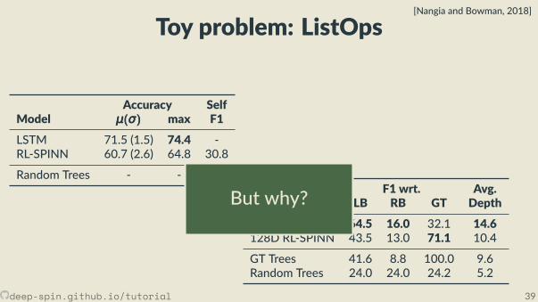
Accuracy SelfModel μ(σ)μ(σ)μ(σ) max F1LSTM 71.5 (1.5) 74.4 -RL-SPINN 60.7 (2.6) 64.8 30.8
Random Trees - - 30.1F1 wrt. Avg.
Model LB RB GT Depth48D RL-SPINN 64.5 16.0 32.1 14.6128D RL-SPINN 43.5 13.0 71.1 10.4
GT Trees 41.6 8.8 100.0 9.6Random Trees 24.0 24.0 24.2 5.2
But why?
deep-spin.github.io/tutorial 39
Toy problem: ListOps[Nangia and Bowman, 2018]
Accuracy SelfModel μ(σ)μ(σ)μ(σ) max F1LSTM 71.5 (1.5) 74.4 -RL-SPINN 60.7 (2.6) 64.8 30.8
Random Trees - - 30.1F1 wrt. Avg.
Model LB RB GT Depth48D RL-SPINN 64.5 16.0 32.1 14.6128D RL-SPINN 43.5 13.0 71.1 10.4
GT Trees 41.6 8.8 100.0 9.6Random Trees 24.0 24.0 24.2 5.2
But why?
deep-spin.github.io/tutorial 39
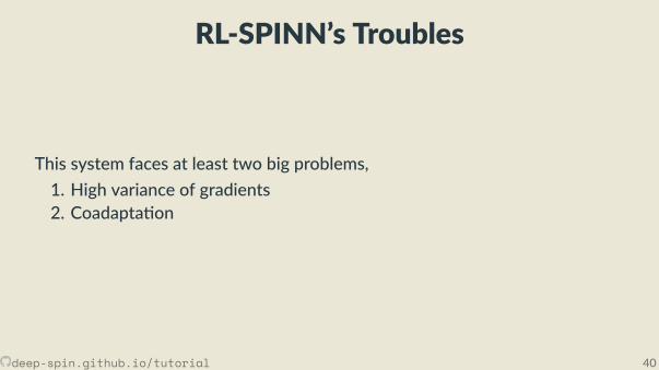
RL-SPINN’s Troubles
This system faces at least two big problems,
1. High variance of gradients2. Coadapta on
deep-spin.github.io/tutorial 40
RL-SPINN’s Troubles
This system faces at least two big problems,1. High variance of gradients2. Coadapta on
deep-spin.github.io/tutorial 40
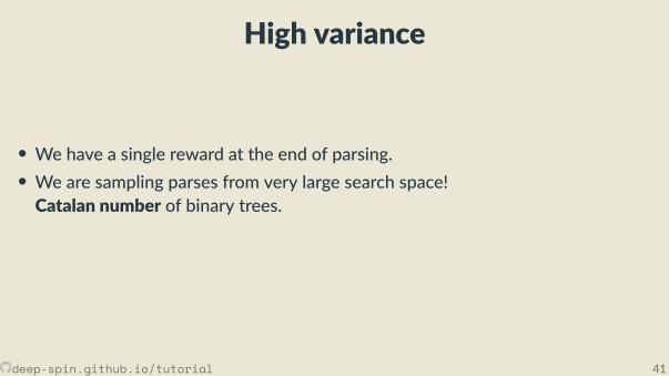
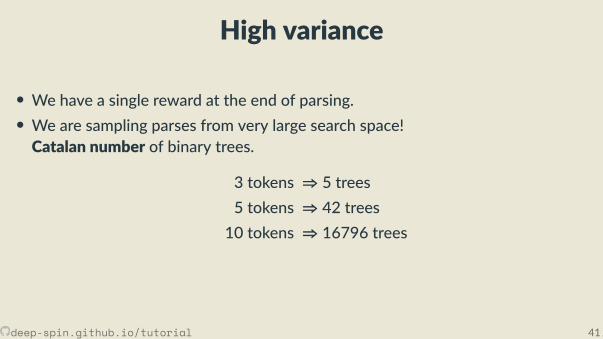
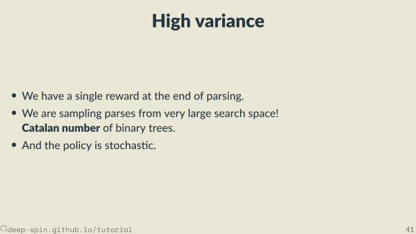
High variance
• We have a single reward at the end of parsing.
• We are sampling parses from very large search space!Catalan number of binary trees.• And the policy is stochas c.
deep-spin.github.io/tutorial 41
High variance
• We have a single reward at the end of parsing.• We are sampling parses from very large search space!Catalan number of binary trees.
• And the policy is stochas c.
deep-spin.github.io/tutorial 41
High variance
• We have a single reward at the end of parsing.• We are sampling parses from very large search space!Catalan number of binary trees.
3 tokens ⇒ 5 trees5 tokens ⇒ 42 trees10 tokens ⇒ 16796 trees
• And the policy is stochas c.
deep-spin.github.io/tutorial 41
High variance
• We have a single reward at the end of parsing.• We are sampling parses from very large search space!Catalan number of binary trees.• And the policy is stochas c.
deep-spin.github.io/tutorial 41
High variance
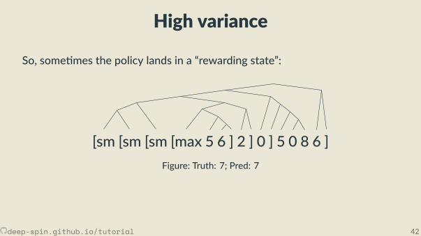
So, some mes the policy lands in a “rewarding state”:
[sm [sm [sm [max 5 6 ] 2 ] 0 ] 5 0 8 6 ]Figure: Truth: 7; Pred: 7
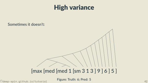
Some mes it doesn’t:
deep-spin.github.io/tutorial 42
High variance
So, some mes the policy lands in a “rewarding state”:
Some mes it doesn’t:
[max [med [med 1 [sm 3 1 3 ] 9 ] 6 ] 5 ]Figure: Truth: 6; Pred: 5deep-spin.github.io/tutorial 42
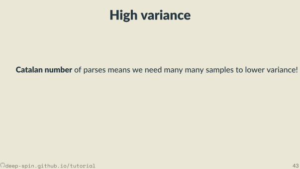
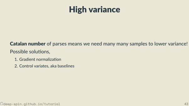
High variance
Catalan number of parses means we need many many samples to lower variance!
Possible solu ons,1. Gradient normaliza on2. Control variates, aka baselines
deep-spin.github.io/tutorial 43
High variance
Catalan number of parses means we need many many samples to lower variance!Possible solu ons,1. Gradient normaliza on2. Control variates, aka baselines
deep-spin.github.io/tutorial 43
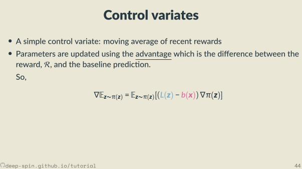
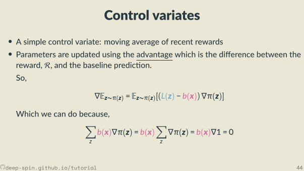
Control variates
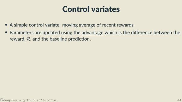
• A simple control variate: moving average of recent rewards
• Parameters are updated using the advantage which is the di erence between thereward, R, and the baseline predic on.So,
∇Ez∼π(z) = Ez∼π(z)[(L(z) − b(x))∇π(z)]
Which we can do because,∑zb(x)∇π(z) = b(x)
∑z∇π(z) = b(x)∇1 = 0
deep-spin.github.io/tutorial 44
Control variates
• A simple control variate: moving average of recent rewards• Parameters are updated using the advantage which is the di erence between thereward, R, and the baseline predic on.
So,
∇Ez∼π(z) = Ez∼π(z)[(L(z) − b(x))∇π(z)]
Which we can do because,∑zb(x)∇π(z) = b(x)
∑z∇π(z) = b(x)∇1 = 0
deep-spin.github.io/tutorial 44
Control variates
• A simple control variate: moving average of recent rewards• Parameters are updated using the advantage which is the di erence between thereward, R, and the baseline predic on.So,
∇Ez∼π(z) = Ez∼π(z)[(L(z) − b(x))∇π(z)]
Which we can do because,∑zb(x)∇π(z) = b(x)
∑z∇π(z) = b(x)∇1 = 0
deep-spin.github.io/tutorial 44

Issues with SPINN with REINFORCE
This system faces two big problems,1. High variance of gradients2. Coadapta on
deep-spin.github.io/tutorial 45
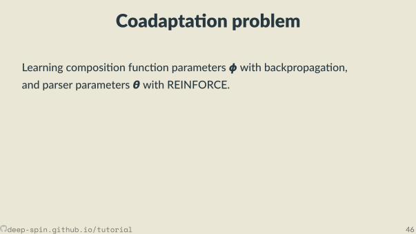
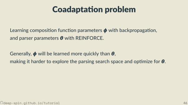
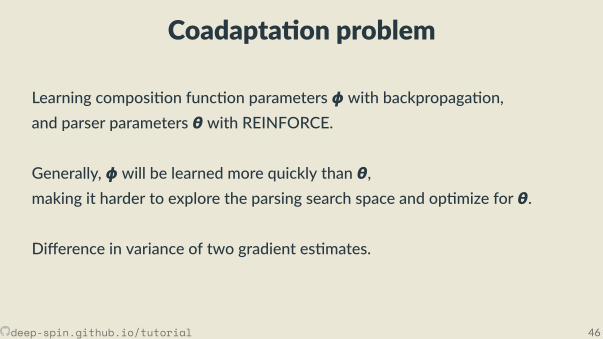
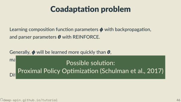
Coadapta on problem
Learning composi on func on parameters φ with backpropaga on,and parser parameters θ with REINFORCE.
Generally, φ will be learned more quickly than θ,making it harder to explore the parsing search space and op mize for θ.
Di erence in variance of two gradient es mates.
Possible solu on:Proximal Policy Op miza on (Schulman et al., 2017)
deep-spin.github.io/tutorial 46
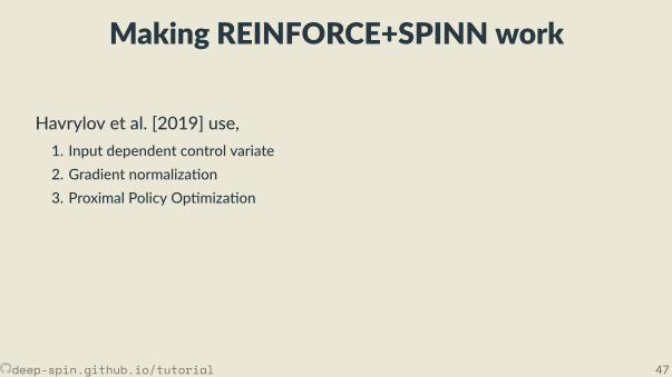
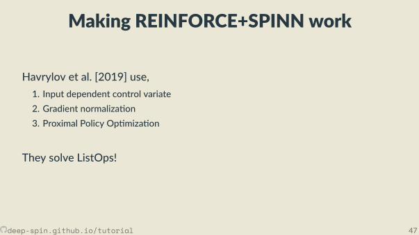
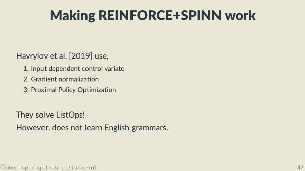
Making REINFORCE+SPINN work
Havrylov et al. [2019] use,1. Input dependent control variate2. Gradient normaliza on3. Proximal Policy Op miza on
They solve ListOps!However, does not learn English grammars.
deep-spin.github.io/tutorial 47
Making REINFORCE+SPINN work
Havrylov et al. [2019] use,1. Input dependent control variate2. Gradient normaliza on3. Proximal Policy Op miza on
They solve ListOps!
However, does not learn English grammars.
deep-spin.github.io/tutorial 47
Making REINFORCE+SPINN work
Havrylov et al. [2019] use,1. Input dependent control variate2. Gradient normaliza on3. Proximal Policy Op miza on
They solve ListOps!However, does not learn English grammars.
deep-spin.github.io/tutorial 47
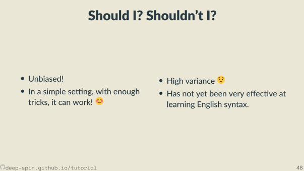
Should I? Shouldn’t I?
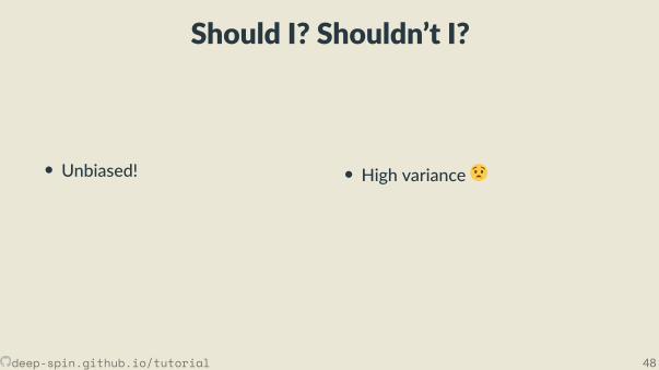
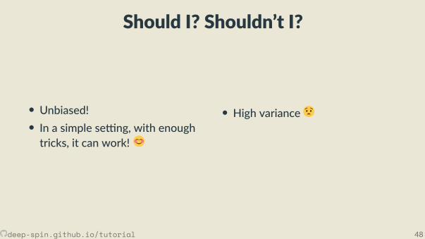
• Unbiased!
• In a simple se ng, with enoughtricks, it can work!
• High variance• Has not yet been very e ec ve atlearning English syntax.
deep-spin.github.io/tutorial 48
Should I? Shouldn’t I?
• Unbiased!
• In a simple se ng, with enoughtricks, it can work!
• High variance
• Has not yet been very e ec ve atlearning English syntax.
deep-spin.github.io/tutorial 48
Should I? Shouldn’t I?
• Unbiased!• In a simple se ng, with enoughtricks, it can work!
• High variance
• Has not yet been very e ec ve atlearning English syntax.
deep-spin.github.io/tutorial 48
Should I? Shouldn’t I?
• Unbiased!• In a simple se ng, with enoughtricks, it can work!
• High variance• Has not yet been very e ec ve atlearning English syntax.
deep-spin.github.io/tutorial 48
III. GradientSurrogates
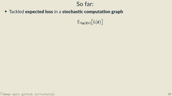
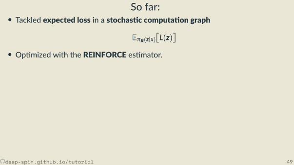
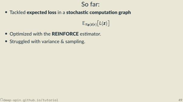
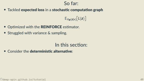
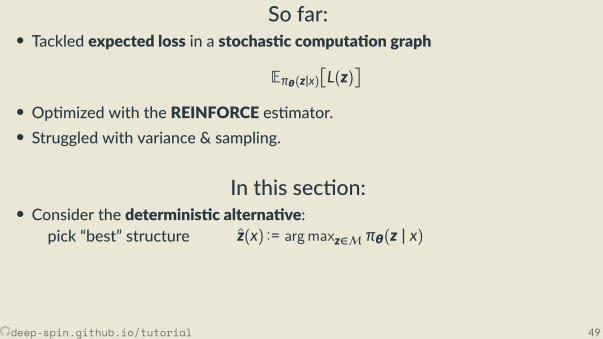
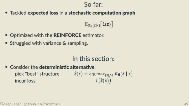
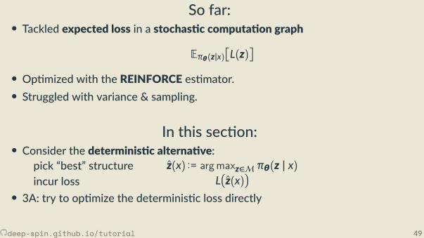
So far:• Tackled expected loss in a stochas c computa on graph
Eπθ(z|x)L(z)
• Op mized with the REINFORCE es mator.• Struggled with variance & sampling.
In this sec on:• Consider the determinis c alterna ve:
pick “best” structure z(x) := argmaxz∈M πθ(z | x)incur loss L
z(x)
• 3A: try to op mize the determinis c loss directly• 3B: use this strategy to reduce variance in the stochas c model.
deep-spin.github.io/tutorial 49
So far:• Tackled expected loss in a stochas c computa on graph
Eπθ(z|x)L(z)
• Op mized with the REINFORCE es mator.
• Struggled with variance & sampling.
In this sec on:• Consider the determinis c alterna ve:
pick “best” structure z(x) := argmaxz∈M πθ(z | x)incur loss L
z(x)
• 3A: try to op mize the determinis c loss directly• 3B: use this strategy to reduce variance in the stochas c model.
deep-spin.github.io/tutorial 49
So far:• Tackled expected loss in a stochas c computa on graph
Eπθ(z|x)L(z)
• Op mized with the REINFORCE es mator.• Struggled with variance & sampling.
In this sec on:• Consider the determinis c alterna ve:
pick “best” structure z(x) := argmaxz∈M πθ(z | x)incur loss L
z(x)
• 3A: try to op mize the determinis c loss directly• 3B: use this strategy to reduce variance in the stochas c model.
deep-spin.github.io/tutorial 49
So far:• Tackled expected loss in a stochas c computa on graph
Eπθ(z|x)L(z)
• Op mized with the REINFORCE es mator.• Struggled with variance & sampling.
In this sec on:• Consider the determinis c alterna ve:
pick “best” structure z(x) := argmaxz∈M πθ(z | x)
incur loss Lz(x)
• 3A: try to op mize the determinis c loss directly• 3B: use this strategy to reduce variance in the stochas c model.
deep-spin.github.io/tutorial 49
So far:• Tackled expected loss in a stochas c computa on graph
Eπθ(z|x)L(z)
• Op mized with the REINFORCE es mator.• Struggled with variance & sampling.
In this sec on:• Consider the determinis c alterna ve:
pick “best” structure z(x) := argmaxz∈M πθ(z | x)incur loss L
z(x)
• 3A: try to op mize the determinis c loss directly• 3B: use this strategy to reduce variance in the stochas c model.
deep-spin.github.io/tutorial 49
So far:• Tackled expected loss in a stochas c computa on graph
Eπθ(z|x)L(z)
• Op mized with the REINFORCE es mator.• Struggled with variance & sampling.
In this sec on:• Consider the determinis c alterna ve:
pick “best” structure z(x) := argmaxz∈M πθ(z | x)incur loss L
z(x)
• 3A: try to op mize the determinis c loss directly
• 3B: use this strategy to reduce variance in the stochas c model.
deep-spin.github.io/tutorial 49
So far:• Tackled expected loss in a stochas c computa on graph
Eπθ(z|x)L(z)
• Op mized with the REINFORCE es mator.• Struggled with variance & sampling.
In this sec on:• Consider the determinis c alterna ve:
pick “best” structure z(x) := argmaxz∈M πθ(z | x)incur loss L
z(x)
• 3A: try to op mize the determinis c loss directly• 3B: use this strategy to reduce variance in the stochas c model.deep-spin.github.io/tutorial 49
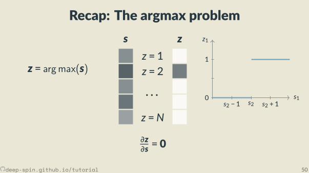
Recap: The argmax problem
z = 1z = 2
· · ·z =N
s z
∂z∂s = 0
z1
s10
1
s2 − 1 s2 s2 + 1
z = argmax(s)
deep-spin.github.io/tutorial 50
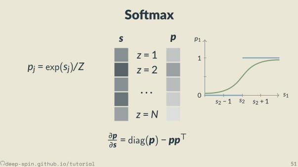
So max
z = 1z = 2
· · ·z =N
s p
∂p∂s = diag(p) − pp
⊤
p1
s10
1
s2 − 1 s2 s2 + 1
pj = exp(sj)/Z
deep-spin.github.io/tutorial 51
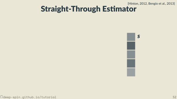
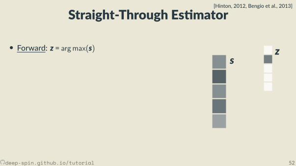
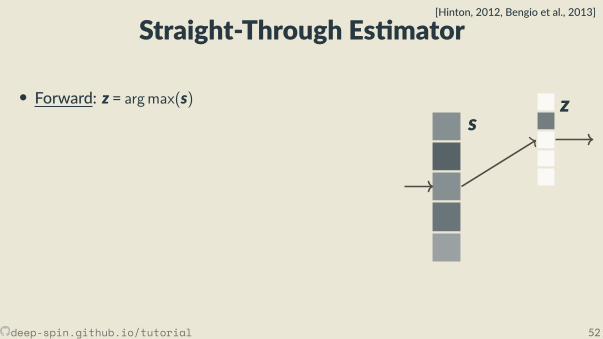
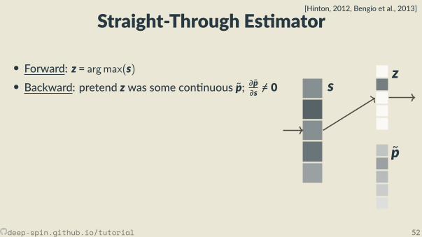
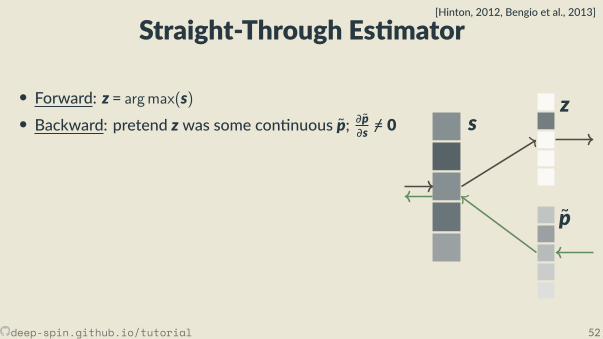
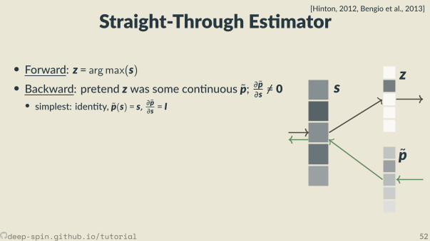
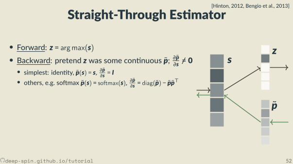
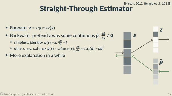
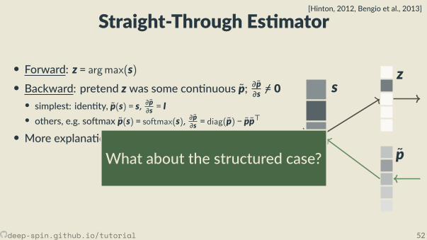
Straight-Through Es mator[Hinton, 2012, Bengio et al., 2013]
• Forward: z = argmax(s)• Backward: pretend z was some con nuous p; ∂p∂s =/ 0
• simplest: iden ty, p(s) = s, ∂p∂s = I• others, e.g. so max p(s) = softmax(s), ∂p∂s = diag(p) − pp⊤
• More explana on in a while
s
z
pWhat about the structured case?
deep-spin.github.io/tutorial 52
Straight-Through Es mator[Hinton, 2012, Bengio et al., 2013]
• Forward: z = argmax(s)
• Backward: pretend z was some con nuous p; ∂p∂s =/ 0
• simplest: iden ty, p(s) = s, ∂p∂s = I• others, e.g. so max p(s) = softmax(s), ∂p∂s = diag(p) − pp⊤
• More explana on in a while
sz
pWhat about the structured case?
deep-spin.github.io/tutorial 52
Straight-Through Es mator[Hinton, 2012, Bengio et al., 2013]
• Forward: z = argmax(s)• Backward: pretend z was some con nuous p; ∂p∂s =/ 0
• simplest: iden ty, p(s) = s, ∂p∂s = I• others, e.g. so max p(s) = softmax(s), ∂p∂s = diag(p) − pp⊤
• More explana on in a while
sz
p
What about the structured case?
deep-spin.github.io/tutorial 52
Straight-Through Es mator[Hinton, 2012, Bengio et al., 2013]
• Forward: z = argmax(s)• Backward: pretend z was some con nuous p; ∂p∂s =/ 0• simplest: iden ty, p(s) = s, ∂p∂s = I
• others, e.g. so max p(s) = softmax(s), ∂p∂s = diag(p) − pp⊤
• More explana on in a while
sz
p
What about the structured case?
deep-spin.github.io/tutorial 52
Straight-Through Es mator[Hinton, 2012, Bengio et al., 2013]
• Forward: z = argmax(s)• Backward: pretend z was some con nuous p; ∂p∂s =/ 0• simplest: iden ty, p(s) = s, ∂p∂s = I• others, e.g. so max p(s) = softmax(s), ∂p∂s = diag(p) − pp
⊤
• More explana on in a while
sz
pWhat about the structured case?
deep-spin.github.io/tutorial 52
Dealing with the combinatorial explosion
→ → → · · ·1. Incremental structures• Build structure greedily, as sequenceof discrete choices (e.g., shi -reduce).• Scores (par al structure, ac on) tuples.• Advantages: exible, rich histories.• Disadvantages: greedy, local decisionsare subop mal, error propaga on.
max · · · , , , , · · ·
2. Factoriza on into parts• Op mizes globally (e.g. Viterbi,Chu-Liu-Edmonds, Kuhn-Munkres).• Scores smaller parts.• Advantages: op mal, elegant, canhandle hard & global constraints.• Disadvantages: strong assump ons.
deep-spin.github.io/tutorial 53
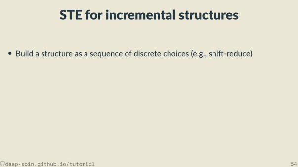
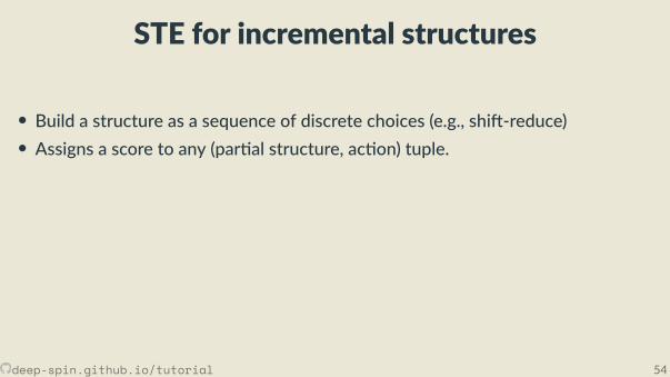
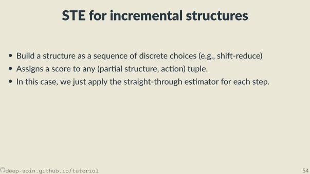
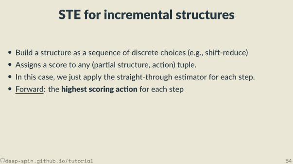
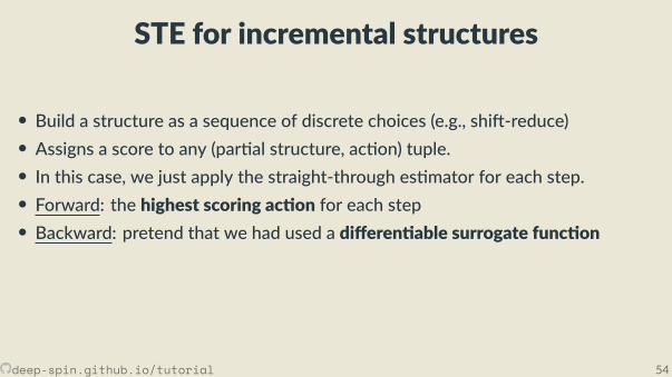
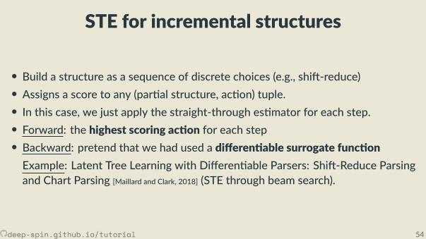
STE for incremental structures
• Build a structure as a sequence of discrete choices (e.g., shi -reduce)• Assigns a score to any (par al structure, ac on) tuple.• In this case, we just apply the straight-through es mator for each step.• Forward: the highest scoring ac on for each step• Backward: pretend that we had used a di eren able surrogate func onExample: Latent Tree Learning with Di eren able Parsers: Shi -Reduce Parsingand Chart Parsing [Maillard and Clark, 2018] (STE through beam search).
deep-spin.github.io/tutorial 54
STE for incremental structures
• Build a structure as a sequence of discrete choices (e.g., shi -reduce)
• Assigns a score to any (par al structure, ac on) tuple.• In this case, we just apply the straight-through es mator for each step.• Forward: the highest scoring ac on for each step• Backward: pretend that we had used a di eren able surrogate func onExample: Latent Tree Learning with Di eren able Parsers: Shi -Reduce Parsingand Chart Parsing [Maillard and Clark, 2018] (STE through beam search).
deep-spin.github.io/tutorial 54
STE for incremental structures
• Build a structure as a sequence of discrete choices (e.g., shi -reduce)• Assigns a score to any (par al structure, ac on) tuple.
• In this case, we just apply the straight-through es mator for each step.• Forward: the highest scoring ac on for each step• Backward: pretend that we had used a di eren able surrogate func onExample: Latent Tree Learning with Di eren able Parsers: Shi -Reduce Parsingand Chart Parsing [Maillard and Clark, 2018] (STE through beam search).
deep-spin.github.io/tutorial 54
STE for incremental structures
• Build a structure as a sequence of discrete choices (e.g., shi -reduce)• Assigns a score to any (par al structure, ac on) tuple.• In this case, we just apply the straight-through es mator for each step.
• Forward: the highest scoring ac on for each step• Backward: pretend that we had used a di eren able surrogate func onExample: Latent Tree Learning with Di eren able Parsers: Shi -Reduce Parsingand Chart Parsing [Maillard and Clark, 2018] (STE through beam search).
deep-spin.github.io/tutorial 54
STE for incremental structures
• Build a structure as a sequence of discrete choices (e.g., shi -reduce)• Assigns a score to any (par al structure, ac on) tuple.• In this case, we just apply the straight-through es mator for each step.• Forward: the highest scoring ac on for each step
• Backward: pretend that we had used a di eren able surrogate func onExample: Latent Tree Learning with Di eren able Parsers: Shi -Reduce Parsingand Chart Parsing [Maillard and Clark, 2018] (STE through beam search).
deep-spin.github.io/tutorial 54
STE for incremental structures
• Build a structure as a sequence of discrete choices (e.g., shi -reduce)• Assigns a score to any (par al structure, ac on) tuple.• In this case, we just apply the straight-through es mator for each step.• Forward: the highest scoring ac on for each step• Backward: pretend that we had used a di eren able surrogate func on
Example: Latent Tree Learning with Di eren able Parsers: Shi -Reduce Parsingand Chart Parsing [Maillard and Clark, 2018] (STE through beam search).
deep-spin.github.io/tutorial 54
STE for incremental structures
• Build a structure as a sequence of discrete choices (e.g., shi -reduce)• Assigns a score to any (par al structure, ac on) tuple.• In this case, we just apply the straight-through es mator for each step.• Forward: the highest scoring ac on for each step• Backward: pretend that we had used a di eren able surrogate func onExample: Latent Tree Learning with Di eren able Parsers: Shi -Reduce Parsingand Chart Parsing [Maillard and Clark, 2018] (STE through beam search).
deep-spin.github.io/tutorial 54
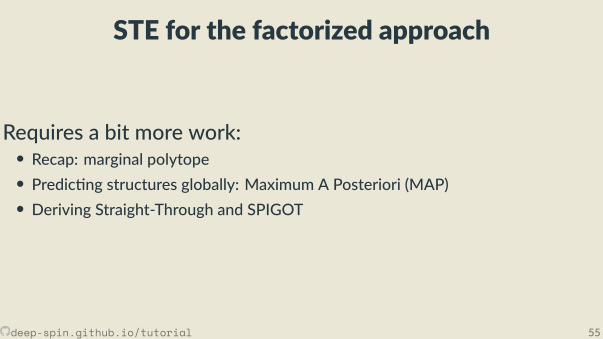
STE for the factorized approach
Requires a bit more work:• Recap: marginal polytope• Predic ng structures globally: Maximum A Posteriori (MAP)• Deriving Straight-Through and SPIGOT
deep-spin.github.io/tutorial 55
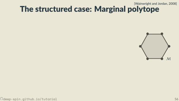
The structured case: Marginal polytope[Wainwright and Jordan, 2008]
• Each vertex corresponds to one such bit vector z• Points inside correspond to marginal distribu ons:convex combina ons of structured objects
μ = p1z1 + . . . + pNzN︸ ︷︷ ︸exponen ally many terms
, p ∈ ∆.
p1 = 0.2, z1 = [1,0,0,0,1,0,0,0,1]p2 = 0.7, z2 = [0,0,1,0,0,1,1,0,0]p3 = 0.1, z3 = [1,0,0,0,1,0,0,1,0]
⇒ μ=[.3,0, .7,0, .3, .7, .7, .1, .2].
M
deep-spin.github.io/tutorial 56

The structured case: Marginal polytope[Wainwright and Jordan, 2008]
• Each vertex corresponds to one such bit vector z
• Points inside correspond to marginal distribu ons:convex combina ons of structured objects
μ = p1z1 + . . . + pNzN︸ ︷︷ ︸exponen ally many terms
, p ∈ ∆.
p1 = 0.2, z1 = [1,0,0,0,1,0,0,0,1]p2 = 0.7, z2 = [0,0,1,0,0,1,1,0,0]p3 = 0.1, z3 = [1,0,0,0,1,0,0,1,0]
⇒ μ=[.3,0, .7,0, .3, .7, .7, .1, .2].
M
deep-spin.github.io/tutorial 56

The structured case: Marginal polytope[Wainwright and Jordan, 2008]
• Each vertex corresponds to one such bit vector z• Points inside correspond to marginal distribu ons:convex combina ons of structured objects
μ = p1z1 + . . . + pNzN︸ ︷︷ ︸exponen ally many terms
, p ∈ ∆.
p1 = 0.2, z1 = [1,0,0,0,1,0,0,0,1]p2 = 0.7, z2 = [0,0,1,0,0,1,1,0,0]p3 = 0.1, z3 = [1,0,0,0,1,0,0,1,0]
⇒ μ=[.3,0, .7,0, .3, .7, .7, .1, .2].
M
deep-spin.github.io/tutorial 56
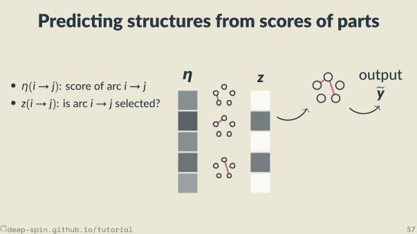
Predic ng structures from scores of parts
• η(i→ j): score of arc i→ j• z(i→ j): is arc i→ j selected?
• Task-speci c algorithm for thehighest-scoring structure.
η z outputey
deep-spin.github.io/tutorial 57
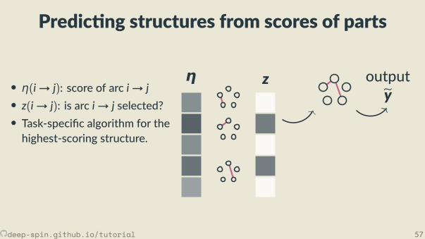
Predic ng structures from scores of parts
• η(i→ j): score of arc i→ j• z(i→ j): is arc i→ j selected?• Task-speci c algorithm for thehighest-scoring structure.
η z outputey
deep-spin.github.io/tutorial 57
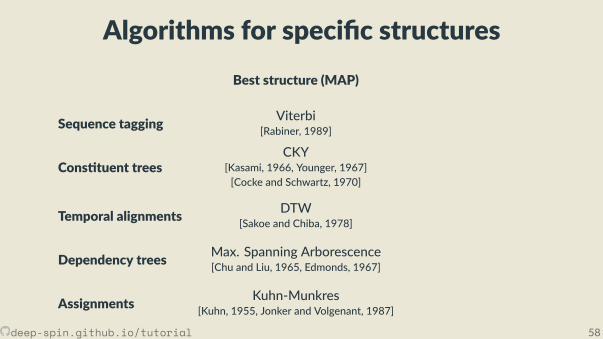
Algorithms for speci c structuresBest structure (MAP)
Marginals
Sequence tagging Viterbi[Rabiner, 1989]
Forward-Backward[Rabiner, 1989]
Cons tuent treesCKY
[Kasami, 1966, Younger, 1967][Cocke and Schwartz, 1970]
Inside-Outside[Baker, 1979]
Temporal alignments DTW[Sakoe and Chiba, 1978]
So -DTW[Cuturi and Blondel, 2017]
Dependency trees Max. Spanning Arborescence[Chu and Liu, 1965, Edmonds, 1967]
Matrix-Tree[Kirchho , 1847]
Assignments Kuhn-Munkres[Kuhn, 1955, Jonker and Volgenant, 1987]
#P-complete[Valiant, 1979, Taskar, 2004]
deep-spin.github.io/tutorial 58
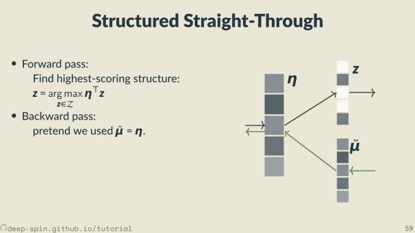
Structured Straight-Through
• Forward pass:Find highest-scoring structure:z = argmax
z∈Zη⊤z
• Backward pass:pretend we used μ =η.
ηz
μ
deep-spin.github.io/tutorial 59
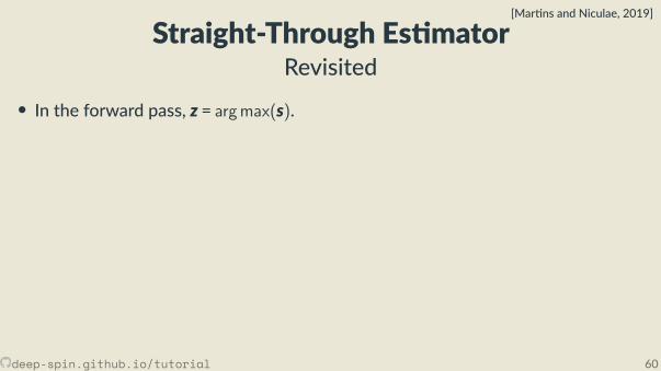
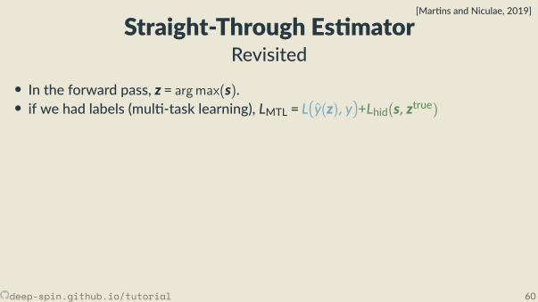
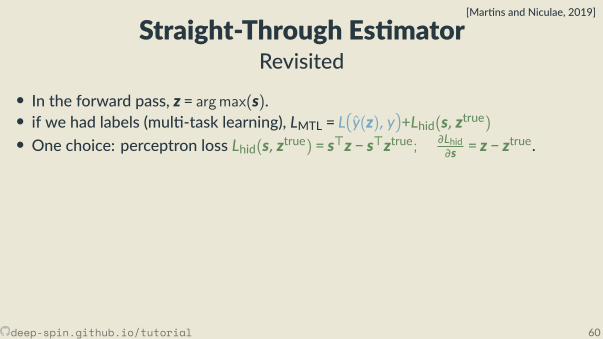
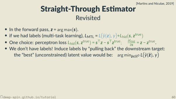
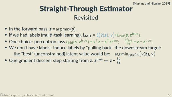
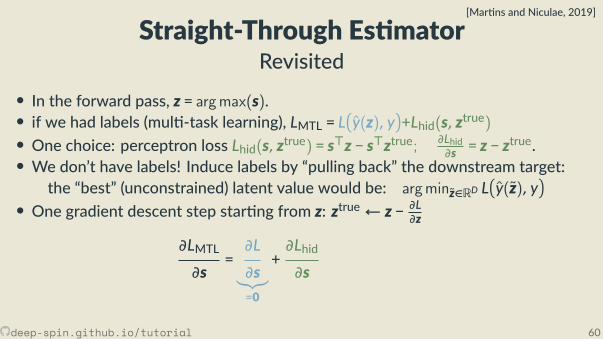
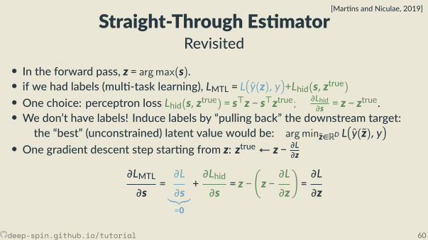
Straight-Through Es matorRevisited
• In the forward pass, z = argmax(s).• if we had labels (mul -task learning), LMTL = Ly(z), y+Lhid(s, ztrue)• One choice: perceptron loss Lhid(s, ztrue) = s⊤z − s⊤ztrue; ∂Lhid
∂s = z − ztrue.
• We don’t have labels! Induce labels by “pulling back” the downstream target:the “best” (unconstrained) latent value would be: argminz∈RD L
y(z), y
• One gradient descent step star ng from z: ztrue← z − ∂L∂z
∂LMTL∂s
=∂L
∂s︸︷︷︸=0
+∂Lhid∂s
= z −z −
∂L
∂z
=∂L
∂z
[Mar ns and Niculae, 2019]
deep-spin.github.io/tutorial 60
Straight-Through Es matorRevisited
• In the forward pass, z = argmax(s).
• if we had labels (mul -task learning), LMTL = Ly(z), y+Lhid(s, ztrue)• One choice: perceptron loss Lhid(s, ztrue) = s⊤z − s⊤ztrue; ∂Lhid
∂s = z − ztrue.
• We don’t have labels! Induce labels by “pulling back” the downstream target:the “best” (unconstrained) latent value would be: argminz∈RD L
y(z), y
• One gradient descent step star ng from z: ztrue← z − ∂L∂z
∂LMTL∂s
=∂L
∂s︸︷︷︸=0
+∂Lhid∂s
= z −z −
∂L
∂z
=∂L
∂z
[Mar ns and Niculae, 2019]
deep-spin.github.io/tutorial 60
Straight-Through Es matorRevisited
• In the forward pass, z = argmax(s).• if we had labels (mul -task learning), LMTL = Ly(z), y+Lhid(s, ztrue)
• One choice: perceptron loss Lhid(s, ztrue) = s⊤z − s⊤ztrue; ∂Lhid∂s = z − z
true.• We don’t have labels! Induce labels by “pulling back” the downstream target:
the “best” (unconstrained) latent value would be: argminz∈RD Ly(z), y
• One gradient descent step star ng from z: ztrue← z − ∂L∂z
∂LMTL∂s
=∂L
∂s︸︷︷︸=0
+∂Lhid∂s
= z −z −
∂L
∂z
=∂L
∂z
[Mar ns and Niculae, 2019]
deep-spin.github.io/tutorial 60
Straight-Through Es matorRevisited
• In the forward pass, z = argmax(s).• if we had labels (mul -task learning), LMTL = Ly(z), y+Lhid(s, ztrue)• One choice: perceptron loss Lhid(s, ztrue) = s⊤z − s⊤ztrue; ∂Lhid
∂s = z − ztrue.
• We don’t have labels! Induce labels by “pulling back” the downstream target:the “best” (unconstrained) latent value would be: argminz∈RD L
y(z), y
• One gradient descent step star ng from z: ztrue← z − ∂L∂z
∂LMTL∂s
=∂L
∂s︸︷︷︸=0
+∂Lhid∂s
= z −z −
∂L
∂z
=∂L
∂z
[Mar ns and Niculae, 2019]
deep-spin.github.io/tutorial 60
Straight-Through Es matorRevisited
• In the forward pass, z = argmax(s).• if we had labels (mul -task learning), LMTL = Ly(z), y+Lhid(s, ztrue)• One choice: perceptron loss Lhid(s, ztrue) = s⊤z − s⊤ztrue; ∂Lhid
∂s = z − ztrue.
• We don’t have labels! Induce labels by “pulling back” the downstream target:the “best” (unconstrained) latent value would be: argminz∈RD L
y(z), y
• One gradient descent step star ng from z: ztrue← z − ∂L∂z
∂LMTL∂s
=∂L
∂s︸︷︷︸=0
+∂Lhid∂s
= z −z −
∂L
∂z
=∂L
∂z
[Mar ns and Niculae, 2019]
deep-spin.github.io/tutorial 60
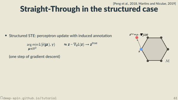
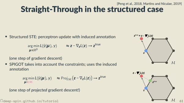
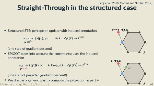
Straight-Through in the structured case[Peng et al., 2018, Mar ns and Niculae, 2019]
• Structured STE: perceptron update with induced annota onargminμ∈RD
L(y(μ), y) ≈ z − ∇zL(z)→ ztrue
(one step of gradient descent)
• SPIGOT takes into account the constraints; uses the inducedannota on
argminμ∈M
L(y(μ), y) ≈ ProjMz − ∇zL(z)→ ztrue
(one step of projected gradient descent!)• We discuss a generic way to compute the projec on in part 4.
z
ztrue = z - ∇zL(z)
z
z - ∇zL(z)
ztrue
deep-spin.github.io/tutorial 61
Straight-Through in the structured case[Peng et al., 2018, Mar ns and Niculae, 2019]
• Structured STE: perceptron update with induced annota onargminμ∈RD
L(y(μ), y) ≈ z − ∇zL(z)→ ztrue
(one step of gradient descent)• SPIGOT takes into account the constraints; uses the inducedannota on
argminμ∈M
L(y(μ), y) ≈ ProjMz − ∇zL(z)→ ztrue
(one step of projected gradient descent!)
• We discuss a generic way to compute the projec on in part 4.
z
ztrue = z - ∇zL(z)
z
z - ∇zL(z)
ztrue
deep-spin.github.io/tutorial 61
Straight-Through in the structured case[Peng et al., 2018, Mar ns and Niculae, 2019]
• Structured STE: perceptron update with induced annota onargminμ∈RD
L(y(μ), y) ≈ z − ∇zL(z)→ ztrue
(one step of gradient descent)• SPIGOT takes into account the constraints; uses the inducedannota on
argminμ∈M
L(y(μ), y) ≈ ProjMz − ∇zL(z)→ ztrue
(one step of projected gradient descent!)• We discuss a generic way to compute the projec on in part 4.
z
ztrue = z - ∇zL(z)
z
z - ∇zL(z)
ztrue
deep-spin.github.io/tutorial 61
Summary: Straight-Through Es mator
We saw how to use the Straight-Through Es mator to allow learning models withargmax in the middle of the computa on graph.We were op mizing L
z(x)
Now we will see how to apply STE for stochas c graphs, as an alterna veapproach of REINFORCE.
deep-spin.github.io/tutorial 62
Summary: Straight-Through Es mator
We saw how to use the Straight-Through Es mator to allow learning models withargmax in the middle of the computa on graph.
We were op mizing Lz(x)
Now we will see how to apply STE for stochas c graphs, as an alterna veapproach of REINFORCE.
deep-spin.github.io/tutorial 62
Summary: Straight-Through Es mator
We saw how to use the Straight-Through Es mator to allow learning models withargmax in the middle of the computa on graph.We were op mizing L
z(x)
Now we will see how to apply STE for stochas c graphs, as an alterna veapproach of REINFORCE.
deep-spin.github.io/tutorial 62
Summary: Straight-Through Es mator
We saw how to use the Straight-Through Es mator to allow learning models withargmax in the middle of the computa on graph.We were op mizing L
z(x)
Now we will see how to apply STE for stochas c graphs, as an alterna veapproach of REINFORCE.
deep-spin.github.io/tutorial 62
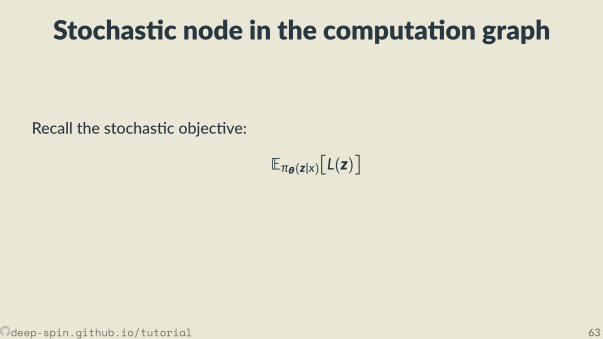
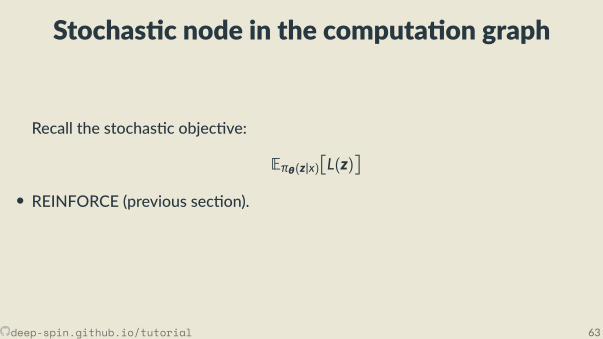
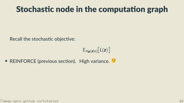
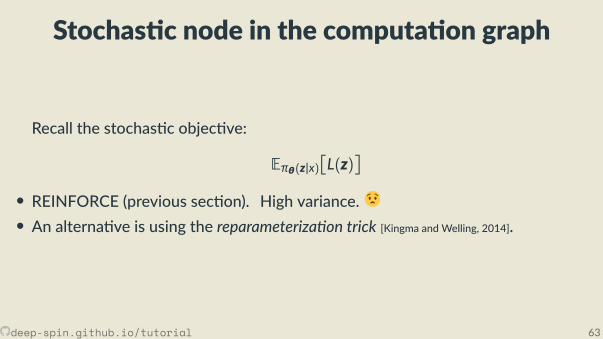
Stochas c node in the computa on graph
Recall the stochas c objec ve:
Eπθ(z|x)L(z)
• REINFORCE (previous sec on).
High variance.
• An alterna ve is using the reparameteriza on trick [Kingma and Welling, 2014].
deep-spin.github.io/tutorial 63
Stochas c node in the computa on graph
Recall the stochas c objec ve:
Eπθ(z|x)L(z)
• REINFORCE (previous sec on).
High variance.
• An alterna ve is using the reparameteriza on trick [Kingma and Welling, 2014].
deep-spin.github.io/tutorial 63
Stochas c node in the computa on graph
Recall the stochas c objec ve:
Eπθ(z|x)L(z)
• REINFORCE (previous sec on).
High variance.• An alterna ve is using the reparameteriza on trick [Kingma and Welling, 2014].
deep-spin.github.io/tutorial 63
Stochas c node in the computa on graph
Recall the stochas c objec ve:
Eπθ(z|x)L(z)
• REINFORCE (previous sec on). High variance.
• An alterna ve is using the reparameteriza on trick [Kingma and Welling, 2014].
deep-spin.github.io/tutorial 63
Stochas c node in the computa on graph
Recall the stochas c objec ve:
Eπθ(z|x)L(z)
• REINFORCE (previous sec on). High variance.• An alterna ve is using the reparameteriza on trick [Kingma and Welling, 2014].
deep-spin.github.io/tutorial 63
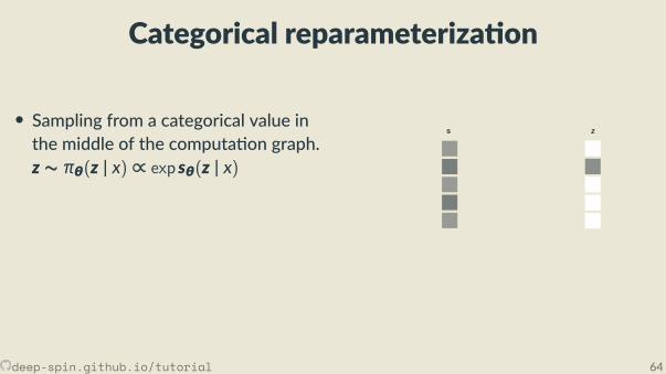
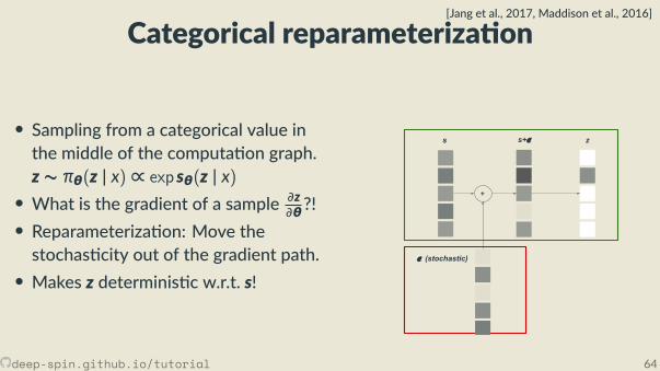
Categorical reparameteriza on
[Jang et al., 2017, Maddison et al., 2016]
• Sampling from a categorical value inthe middle of the computa on graph.z ∼ πθ(z | x) ∝ exp sθ(z | x)• What is the gradient of a sample ∂z
∂θ?!• Reparameteriza on: Move thestochas city out of the gradient path.• Makes z determinis c w.r.t. s!
deep-spin.github.io/tutorial 64
Categorical reparameteriza on
[Jang et al., 2017, Maddison et al., 2016]
• Sampling from a categorical value inthe middle of the computa on graph.z ∼ πθ(z | x) ∝ exp sθ(z | x)
• What is the gradient of a sample ∂z∂θ?!• Reparameteriza on: Move the
stochas city out of the gradient path.• Makes z determinis c w.r.t. s!
s z
deep-spin.github.io/tutorial 64
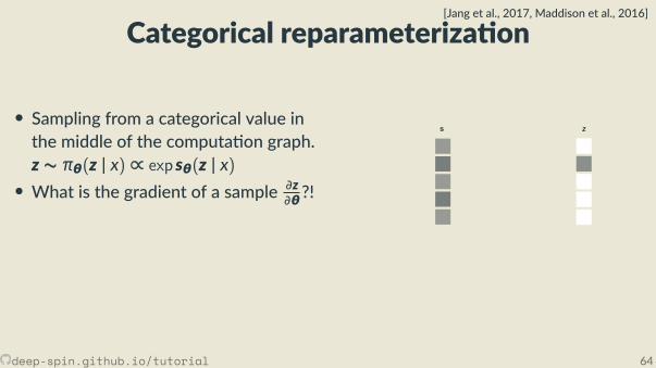
Categorical reparameteriza on[Jang et al., 2017, Maddison et al., 2016]
• Sampling from a categorical value inthe middle of the computa on graph.z ∼ πθ(z | x) ∝ exp sθ(z | x)• What is the gradient of a sample ∂z
∂θ?!
• Reparameteriza on: Move thestochas city out of the gradient path.• Makes z determinis c w.r.t. s!
s z
deep-spin.github.io/tutorial 64
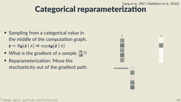
Categorical reparameteriza on[Jang et al., 2017, Maddison et al., 2016]
• Sampling from a categorical value inthe middle of the computa on graph.z ∼ πθ(z | x) ∝ exp sθ(z | x)• What is the gradient of a sample ∂z
∂θ?!• Reparameteriza on: Move thestochas city out of the gradient path.
• Makes z determinis c w.r.t. s!
s
𝝐 (stochastic)
z
deep-spin.github.io/tutorial 64
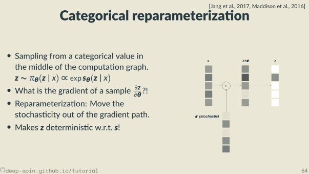
Categorical reparameteriza on[Jang et al., 2017, Maddison et al., 2016]
• Sampling from a categorical value inthe middle of the computa on graph.z ∼ πθ(z | x) ∝ exp sθ(z | x)• What is the gradient of a sample ∂z
∂θ?!• Reparameteriza on: Move thestochas city out of the gradient path.• Makes z determinis c w.r.t. s!
s+𝝐s
𝝐 (stochastic)
+
z
deep-spin.github.io/tutorial 64
Categorical reparameteriza on[Jang et al., 2017, Maddison et al., 2016]
• Sampling from a categorical value inthe middle of the computa on graph.z ∼ πθ(z | x) ∝ exp sθ(z | x)• What is the gradient of a sample ∂z
∂θ?!• Reparameteriza on: Move thestochas city out of the gradient path.• Makes z determinis c w.r.t. s!
s+𝝐s
𝝐 (stochastic)
+
z
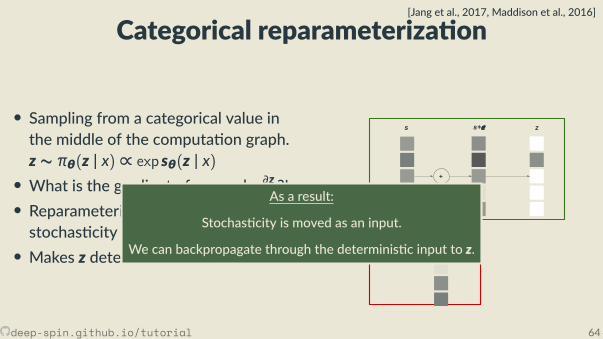
As a result:
Stochas city is moved as an input.
We can backpropagate through the determinis c input to z.
deep-spin.github.io/tutorial 64
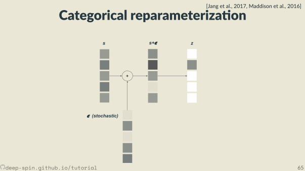
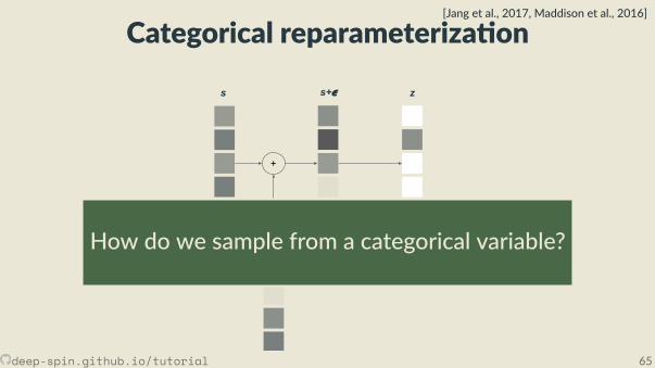
Categorical reparameteriza on[Jang et al., 2017, Maddison et al., 2016]
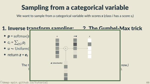
s+𝝐s
𝝐 (stochastic)
+
z
How do we sample from a categorical variable?
deep-spin.github.io/tutorial 65
Categorical reparameteriza on[Jang et al., 2017, Maddison et al., 2016]
s+𝝐s
𝝐 (stochastic)
+
z
How do we sample from a categorical variable?
deep-spin.github.io/tutorial 65
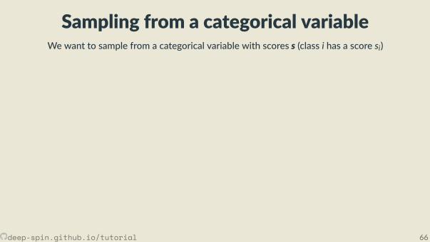
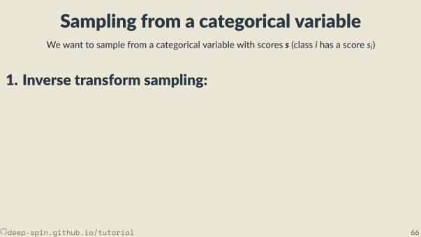
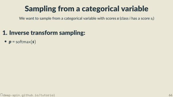
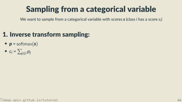
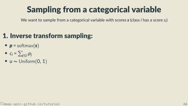
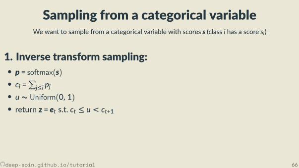
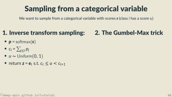
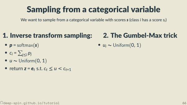
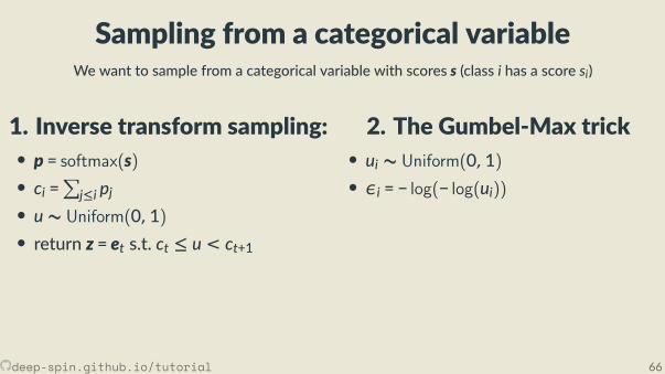
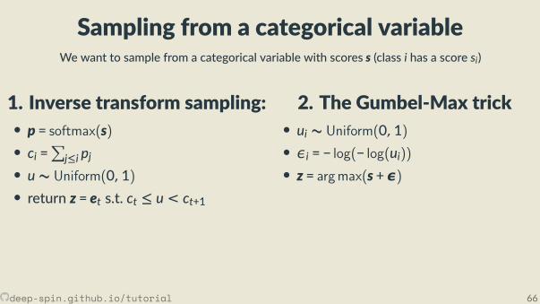
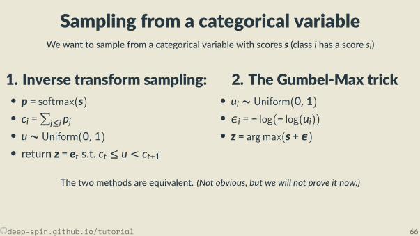
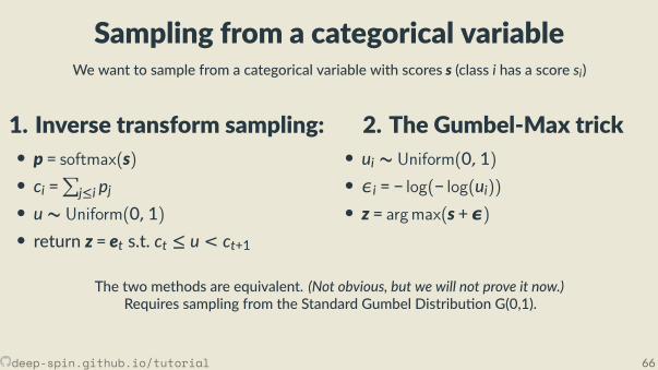
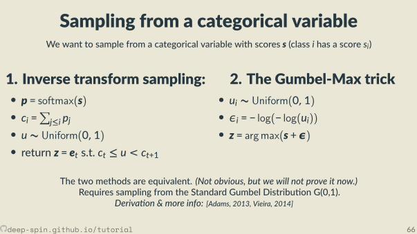
Sampling from a categorical variableWe want to sample from a categorical variable with scores s (class i has a score si)
1. Inverse transform sampling:• p = softmax(s)• ci =∑
j≤i pj• u ∼ Uniform(0,1)• return z = et s.t. ct ≤ u < ct+1
2. The Gumbel-Max trick• ui ∼ Uniform(0,1)• εi = − log(− log(ui))• z = argmax(s + ε)
The two methods are equivalent. (Not obvious, but we will not prove it now.)Requires sampling from the Standard Gumbel Distribu on G(0,1).
Deriva on & more info: [Adams, 2013, Vieira, 2014]
s+𝝐s
𝝐 (stochastic)
+
z
We have an argmax againand cannot backpropagate!
deep-spin.github.io/tutorial 66
Sampling from a categorical variableWe want to sample from a categorical variable with scores s (class i has a score si)
1. Inverse transform sampling:
• p = softmax(s)• ci =∑
j≤i pj• u ∼ Uniform(0,1)• return z = et s.t. ct ≤ u < ct+1
2. The Gumbel-Max trick• ui ∼ Uniform(0,1)• εi = − log(− log(ui))• z = argmax(s + ε)
The two methods are equivalent. (Not obvious, but we will not prove it now.)Requires sampling from the Standard Gumbel Distribu on G(0,1).
Deriva on & more info: [Adams, 2013, Vieira, 2014]
s+𝝐s
𝝐 (stochastic)
+
z
We have an argmax againand cannot backpropagate!
deep-spin.github.io/tutorial 66
Sampling from a categorical variableWe want to sample from a categorical variable with scores s (class i has a score si)
1. Inverse transform sampling:• p = softmax(s)
• ci =∑
j≤i pj• u ∼ Uniform(0,1)• return z = et s.t. ct ≤ u < ct+1
2. The Gumbel-Max trick• ui ∼ Uniform(0,1)• εi = − log(− log(ui))• z = argmax(s + ε)
The two methods are equivalent. (Not obvious, but we will not prove it now.)Requires sampling from the Standard Gumbel Distribu on G(0,1).
Deriva on & more info: [Adams, 2013, Vieira, 2014]
s+𝝐s
𝝐 (stochastic)
+
z
We have an argmax againand cannot backpropagate!
deep-spin.github.io/tutorial 66
Sampling from a categorical variableWe want to sample from a categorical variable with scores s (class i has a score si)
1. Inverse transform sampling:• p = softmax(s)• ci =∑
j≤i pj
• u ∼ Uniform(0,1)• return z = et s.t. ct ≤ u < ct+1
2. The Gumbel-Max trick• ui ∼ Uniform(0,1)• εi = − log(− log(ui))• z = argmax(s + ε)
The two methods are equivalent. (Not obvious, but we will not prove it now.)Requires sampling from the Standard Gumbel Distribu on G(0,1).
Deriva on & more info: [Adams, 2013, Vieira, 2014]
s+𝝐s
𝝐 (stochastic)
+
z
We have an argmax againand cannot backpropagate!
deep-spin.github.io/tutorial 66
Sampling from a categorical variableWe want to sample from a categorical variable with scores s (class i has a score si)
1. Inverse transform sampling:• p = softmax(s)• ci =∑
j≤i pj• u ∼ Uniform(0,1)
• return z = et s.t. ct ≤ u < ct+1
2. The Gumbel-Max trick• ui ∼ Uniform(0,1)• εi = − log(− log(ui))• z = argmax(s + ε)
The two methods are equivalent. (Not obvious, but we will not prove it now.)Requires sampling from the Standard Gumbel Distribu on G(0,1).
Deriva on & more info: [Adams, 2013, Vieira, 2014]
s+𝝐s
𝝐 (stochastic)
+
z
We have an argmax againand cannot backpropagate!
deep-spin.github.io/tutorial 66
Sampling from a categorical variableWe want to sample from a categorical variable with scores s (class i has a score si)
1. Inverse transform sampling:• p = softmax(s)• ci =∑
j≤i pj• u ∼ Uniform(0,1)• return z = et s.t. ct ≤ u < ct+1
2. The Gumbel-Max trick• ui ∼ Uniform(0,1)• εi = − log(− log(ui))• z = argmax(s + ε)
The two methods are equivalent. (Not obvious, but we will not prove it now.)Requires sampling from the Standard Gumbel Distribu on G(0,1).
Deriva on & more info: [Adams, 2013, Vieira, 2014]
s+𝝐s
𝝐 (stochastic)
+
z
We have an argmax againand cannot backpropagate!
deep-spin.github.io/tutorial 66
Sampling from a categorical variableWe want to sample from a categorical variable with scores s (class i has a score si)
1. Inverse transform sampling:• p = softmax(s)• ci =∑
j≤i pj• u ∼ Uniform(0,1)• return z = et s.t. ct ≤ u < ct+1
2. The Gumbel-Max trick
• ui ∼ Uniform(0,1)• εi = − log(− log(ui))• z = argmax(s + ε)
The two methods are equivalent. (Not obvious, but we will not prove it now.)Requires sampling from the Standard Gumbel Distribu on G(0,1).
Deriva on & more info: [Adams, 2013, Vieira, 2014]
s+𝝐s
𝝐 (stochastic)
+
z
We have an argmax againand cannot backpropagate!
deep-spin.github.io/tutorial 66
Sampling from a categorical variableWe want to sample from a categorical variable with scores s (class i has a score si)
1. Inverse transform sampling:• p = softmax(s)• ci =∑
j≤i pj• u ∼ Uniform(0,1)• return z = et s.t. ct ≤ u < ct+1
2. The Gumbel-Max trick• ui ∼ Uniform(0,1)
• εi = − log(− log(ui))• z = argmax(s + ε)
The two methods are equivalent. (Not obvious, but we will not prove it now.)Requires sampling from the Standard Gumbel Distribu on G(0,1).
Deriva on & more info: [Adams, 2013, Vieira, 2014]
s+𝝐s
𝝐 (stochastic)
+
z
We have an argmax againand cannot backpropagate!
deep-spin.github.io/tutorial 66
Sampling from a categorical variableWe want to sample from a categorical variable with scores s (class i has a score si)
1. Inverse transform sampling:• p = softmax(s)• ci =∑
j≤i pj• u ∼ Uniform(0,1)• return z = et s.t. ct ≤ u < ct+1
2. The Gumbel-Max trick• ui ∼ Uniform(0,1)• εi = − log(− log(ui))
• z = argmax(s + ε)
The two methods are equivalent. (Not obvious, but we will not prove it now.)Requires sampling from the Standard Gumbel Distribu on G(0,1).
Deriva on & more info: [Adams, 2013, Vieira, 2014]
s+𝝐s
𝝐 (stochastic)
+
z
We have an argmax againand cannot backpropagate!
deep-spin.github.io/tutorial 66
Sampling from a categorical variableWe want to sample from a categorical variable with scores s (class i has a score si)
1. Inverse transform sampling:• p = softmax(s)• ci =∑
j≤i pj• u ∼ Uniform(0,1)• return z = et s.t. ct ≤ u < ct+1
2. The Gumbel-Max trick• ui ∼ Uniform(0,1)• εi = − log(− log(ui))• z = argmax(s + ε)
The two methods are equivalent. (Not obvious, but we will not prove it now.)Requires sampling from the Standard Gumbel Distribu on G(0,1).
Deriva on & more info: [Adams, 2013, Vieira, 2014]
s+𝝐s
𝝐 (stochastic)
+
z
We have an argmax againand cannot backpropagate!
deep-spin.github.io/tutorial 66
Sampling from a categorical variableWe want to sample from a categorical variable with scores s (class i has a score si)
1. Inverse transform sampling:• p = softmax(s)• ci =∑
j≤i pj• u ∼ Uniform(0,1)• return z = et s.t. ct ≤ u < ct+1
2. The Gumbel-Max trick• ui ∼ Uniform(0,1)• εi = − log(− log(ui))• z = argmax(s + ε)
The two methods are equivalent. (Not obvious, but we will not prove it now.)
Requires sampling from the Standard Gumbel Distribu on G(0,1).Deriva on & more info: [Adams, 2013, Vieira, 2014]
s+𝝐s
𝝐 (stochastic)
+
z
We have an argmax againand cannot backpropagate!
deep-spin.github.io/tutorial 66
Sampling from a categorical variableWe want to sample from a categorical variable with scores s (class i has a score si)
1. Inverse transform sampling:• p = softmax(s)• ci =∑
j≤i pj• u ∼ Uniform(0,1)• return z = et s.t. ct ≤ u < ct+1
2. The Gumbel-Max trick• ui ∼ Uniform(0,1)• εi = − log(− log(ui))• z = argmax(s + ε)
The two methods are equivalent. (Not obvious, but we will not prove it now.)Requires sampling from the Standard Gumbel Distribu on G(0,1).
Deriva on & more info: [Adams, 2013, Vieira, 2014]
s+𝝐s
𝝐 (stochastic)
+
z
We have an argmax againand cannot backpropagate!
deep-spin.github.io/tutorial 66
Sampling from a categorical variableWe want to sample from a categorical variable with scores s (class i has a score si)
1. Inverse transform sampling:• p = softmax(s)• ci =∑
j≤i pj• u ∼ Uniform(0,1)• return z = et s.t. ct ≤ u < ct+1
2. The Gumbel-Max trick• ui ∼ Uniform(0,1)• εi = − log(− log(ui))• z = argmax(s + ε)
The two methods are equivalent. (Not obvious, but we will not prove it now.)Requires sampling from the Standard Gumbel Distribu on G(0,1).
Deriva on & more info: [Adams, 2013, Vieira, 2014]
s+𝝐s
𝝐 (stochastic)
+
z
We have an argmax againand cannot backpropagate!
deep-spin.github.io/tutorial 66
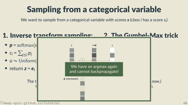
Straight-Through Gumbel Es matorApply a variant of the Straight-Through Es mator to Gumbel-Max!
[Jang et al., 2017, Maddison et al., 2016]
• Forward: z = argmax(s + ε)• Backward: pretend we haddonep = softmax(s + ε)
What about the structured case?
deep-spin.github.io/tutorial 67
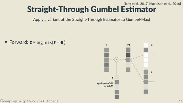
Straight-Through Gumbel Es matorApply a variant of the Straight-Through Es mator to Gumbel-Max!
[Jang et al., 2017, Maddison et al., 2016]
• Forward: z = argmax(s + ε)
• Backward: pretend we haddonep = softmax(s + ε)
s+𝝐s
𝝐
𝝐i =-log(-log(ui))ui~U(0,1)
+
z
p
What about the structured case?
deep-spin.github.io/tutorial 67
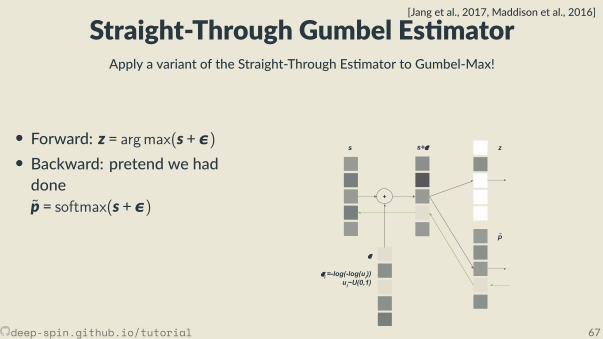
Straight-Through Gumbel Es matorApply a variant of the Straight-Through Es mator to Gumbel-Max!
[Jang et al., 2017, Maddison et al., 2016]
• Forward: z = argmax(s + ε)• Backward: pretend we haddonep = softmax(s + ε)
s+𝝐s
𝝐
𝝐i =-log(-log(ui))ui~U(0,1)
+
z
p
What about the structured case?
deep-spin.github.io/tutorial 67
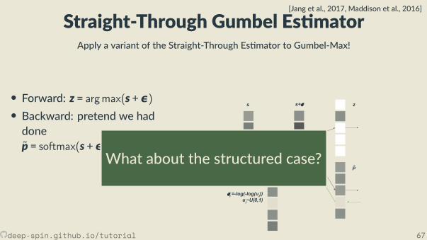
Straight-Through Gumbel Es matorApply a variant of the Straight-Through Es mator to Gumbel-Max!
[Jang et al., 2017, Maddison et al., 2016]
• Forward: z = argmax(s + ε)• Backward: pretend we haddonep = softmax(s + ε)
s+𝝐s
𝝐
𝝐i =-log(-log(ui))ui~U(0,1)
+
z
pWhat about the structured case?
deep-spin.github.io/tutorial 67

Dealing with the combinatorial explosion
→ → → · · ·1. Incremental structures• Build structure greedily, as sequenceof discrete choices (e.g., shi -reduce).• Scores (par al structure, ac on) tuples.• Advantages: exible, rich histories.• Disadvantages: greedy, local decisionsare subop mal, error propaga on.
max · · · , , , , · · ·
2. Factoriza on into parts• Op mizes globally (e.g. Viterbi,Chu-Liu-Edmonds, Kuhn-Munkres).• Scores smaller parts.• Advantages: op mal, elegant, canhandle hard & global constraints.• Disadvantages: strong assump ons.
deep-spin.github.io/tutorial 68
Sampling from incremental structures
• Build a structure as a sequence of discrete choices (e.g., shi -reduce)• Assigns a score to any (par al structure, ac on) tuple.• Reparameterize the scores with Gumbel-Max - now we have a determinis c node.• Forward: the argmax from the reparameterized scores for each step• Backward: pretend we had used a di eren able surrogate func onExample: Gumbel Tree-LSTM [Choi et al., 2018].
deep-spin.github.io/tutorial 69
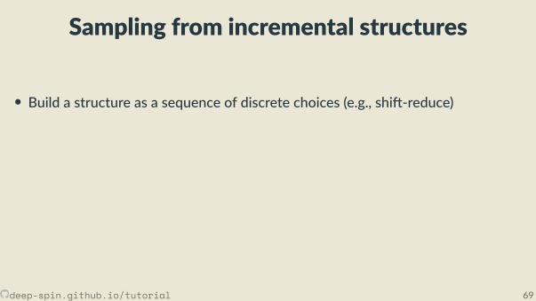
Sampling from incremental structures
• Build a structure as a sequence of discrete choices (e.g., shi -reduce)
• Assigns a score to any (par al structure, ac on) tuple.• Reparameterize the scores with Gumbel-Max - now we have a determinis c node.• Forward: the argmax from the reparameterized scores for each step• Backward: pretend we had used a di eren able surrogate func onExample: Gumbel Tree-LSTM [Choi et al., 2018].
deep-spin.github.io/tutorial 69
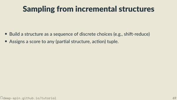
Sampling from incremental structures
• Build a structure as a sequence of discrete choices (e.g., shi -reduce)• Assigns a score to any (par al structure, ac on) tuple.
• Reparameterize the scores with Gumbel-Max - now we have a determinis c node.• Forward: the argmax from the reparameterized scores for each step• Backward: pretend we had used a di eren able surrogate func onExample: Gumbel Tree-LSTM [Choi et al., 2018].
deep-spin.github.io/tutorial 69
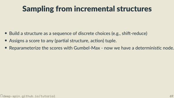
Sampling from incremental structures
• Build a structure as a sequence of discrete choices (e.g., shi -reduce)• Assigns a score to any (par al structure, ac on) tuple.• Reparameterize the scores with Gumbel-Max - now we have a determinis c node.
• Forward: the argmax from the reparameterized scores for each step• Backward: pretend we had used a di eren able surrogate func onExample: Gumbel Tree-LSTM [Choi et al., 2018].
deep-spin.github.io/tutorial 69
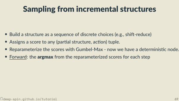
Sampling from incremental structures
• Build a structure as a sequence of discrete choices (e.g., shi -reduce)• Assigns a score to any (par al structure, ac on) tuple.• Reparameterize the scores with Gumbel-Max - now we have a determinis c node.• Forward: the argmax from the reparameterized scores for each step
• Backward: pretend we had used a di eren able surrogate func onExample: Gumbel Tree-LSTM [Choi et al., 2018].
deep-spin.github.io/tutorial 69
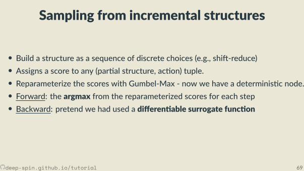
Sampling from incremental structures
• Build a structure as a sequence of discrete choices (e.g., shi -reduce)• Assigns a score to any (par al structure, ac on) tuple.• Reparameterize the scores with Gumbel-Max - now we have a determinis c node.• Forward: the argmax from the reparameterized scores for each step• Backward: pretend we had used a di eren able surrogate func on
Example: Gumbel Tree-LSTM [Choi et al., 2018].
deep-spin.github.io/tutorial 69
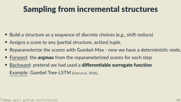
Sampling from incremental structures
• Build a structure as a sequence of discrete choices (e.g., shi -reduce)• Assigns a score to any (par al structure, ac on) tuple.• Reparameterize the scores with Gumbel-Max - now we have a determinis c node.• Forward: the argmax from the reparameterized scores for each step• Backward: pretend we had used a di eren able surrogate func onExample: Gumbel Tree-LSTM [Choi et al., 2018].
deep-spin.github.io/tutorial 69
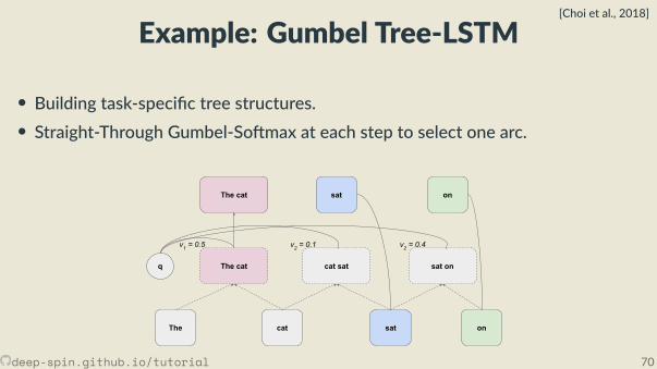
Example: Gumbel Tree-LSTM[Choi et al., 2018]
• Building task-speci c tree structures.• Straight-Through Gumbel-So max at each step to select one arc.
The cat sat on
The cat cat sat sat on
The cat sat on
v1 = 0.5 v2 = 0.1 v2 = 0.4
q
deep-spin.github.io/tutorial 70
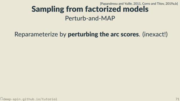
Sampling from factorized modelsPerturb-and-MAP
[Papandreou and Yuille, 2011, Corro and Titov, 2019a,b]
Reparameterize by perturbing the arc scores. (inexact!)
• Sample from the normal Gumbel distribu on.• Perturb the arc scores with the Gumbel noise.• Compute MAP (task-speci c algorithm).• Backward: we could use Straight-Through withIden ty.
• ε ∼ G(0,1)• η =η + ε• argmaxz∈Z η⊤z
deep-spin.github.io/tutorial 71
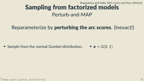
Sampling from factorized modelsPerturb-and-MAP
[Papandreou and Yuille, 2011, Corro and Titov, 2019a,b]
Reparameterize by perturbing the arc scores. (inexact!)
• Sample from the normal Gumbel distribu on.
• Perturb the arc scores with the Gumbel noise.• Compute MAP (task-speci c algorithm).• Backward: we could use Straight-Through withIden ty.
• ε ∼ G(0,1)
• η =η + ε• argmaxz∈Z η⊤z
deep-spin.github.io/tutorial 71
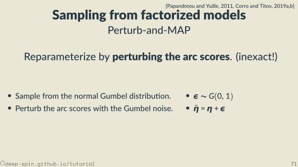
Sampling from factorized modelsPerturb-and-MAP
[Papandreou and Yuille, 2011, Corro and Titov, 2019a,b]
Reparameterize by perturbing the arc scores. (inexact!)
• Sample from the normal Gumbel distribu on.• Perturb the arc scores with the Gumbel noise.
• Compute MAP (task-speci c algorithm).• Backward: we could use Straight-Through withIden ty.
• ε ∼ G(0,1)• η =η + ε
• argmaxz∈Z η⊤z
deep-spin.github.io/tutorial 71
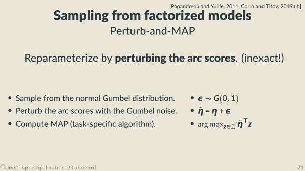
Sampling from factorized modelsPerturb-and-MAP
[Papandreou and Yuille, 2011, Corro and Titov, 2019a,b]
Reparameterize by perturbing the arc scores. (inexact!)
• Sample from the normal Gumbel distribu on.• Perturb the arc scores with the Gumbel noise.• Compute MAP (task-speci c algorithm).
• Backward: we could use Straight-Through withIden ty.
• ε ∼ G(0,1)• η =η + ε• argmaxz∈Z η⊤z
deep-spin.github.io/tutorial 71
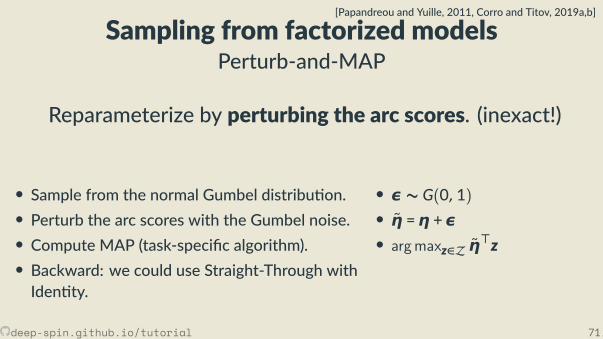
Sampling from factorized modelsPerturb-and-MAP
[Papandreou and Yuille, 2011, Corro and Titov, 2019a,b]
Reparameterize by perturbing the arc scores. (inexact!)
• Sample from the normal Gumbel distribu on.• Perturb the arc scores with the Gumbel noise.• Compute MAP (task-speci c algorithm).• Backward: we could use Straight-Through withIden ty.
• ε ∼ G(0,1)• η =η + ε• argmaxz∈Z η⊤z
deep-spin.github.io/tutorial 71
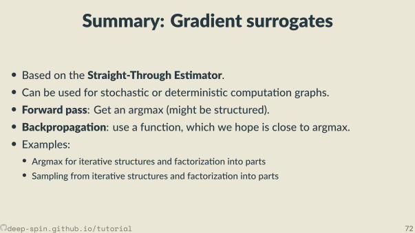
Summary: Gradient surrogates
• Based on the Straight-Through Es mator.• Can be used for stochas c or determinis c computa on graphs.• Forward pass: Get an argmax (might be structured).• Backpropaga on: use a func on, which we hope is close to argmax.• Examples:• Argmax for itera ve structures and factoriza on into parts• Sampling from itera ve structures and factoriza on into parts
deep-spin.github.io/tutorial 72
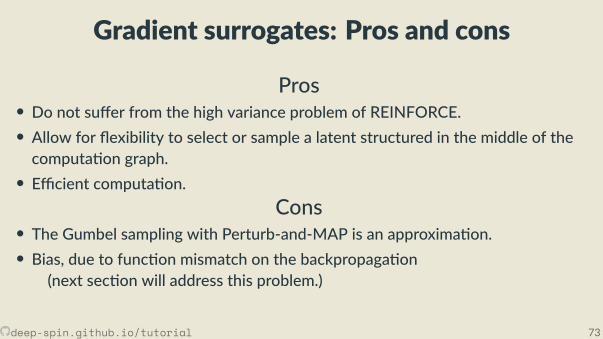
Gradient surrogates: Pros and cons
Pros• Do not su er from the high variance problem of REINFORCE.• Allow for exibility to select or sample a latent structured in the middle of thecomputa on graph.• E cient computa on.
Cons• The Gumbel sampling with Perturb-and-MAP is an approxima on.• Bias, due to func on mismatch on the backpropaga on
(next sec on will address this problem.)
deep-spin.github.io/tutorial 73
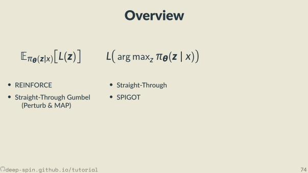
Overview
Eπθ(z|x)L(z)
• REINFORCE• Straight-Through Gumbel
(Perturb & MAP)
• SparseMAP
Largmaxz πθ(z | x)
• Straight-Through• SPIGOT
LEπθ(z|x)[z]
• Structured A n. Nets• SparseMAP
And more, a er the break!
deep-spin.github.io/tutorial 74
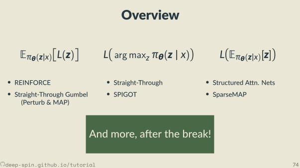
Overview
Eπθ(z|x)L(z)
• REINFORCE• Straight-Through Gumbel
(Perturb & MAP)
• SparseMAP
Largmaxz πθ(z | x)
• Straight-Through• SPIGOT
LEπθ(z|x)[z]
• Structured A n. Nets• SparseMAP
And more, a er the break!
deep-spin.github.io/tutorial 74
IV. End-to-endDi eren ableRelaxa ons
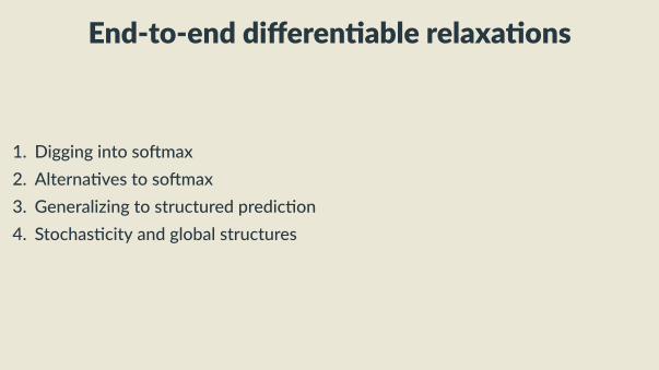
End-to-end di eren able relaxa ons
1. Digging into so max2. Alterna ves to so max3. Generalizing to structured predic on4. Stochas city and global structures
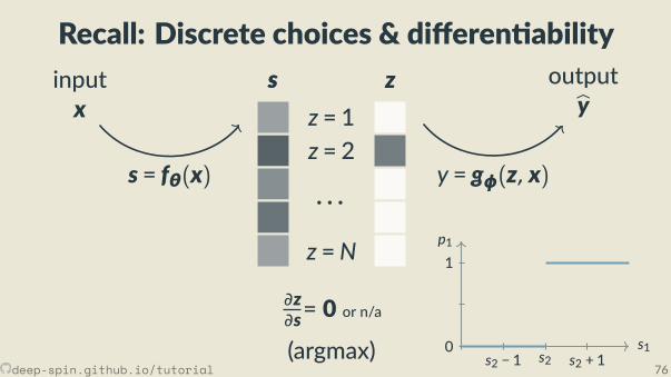
Recall: Discrete choices & di eren abilitys
z = 1z = 2
· · ·z =N
s z
p
∂z∂s= 0 or n/a
inputx
outputbys = fθ(x) y = gφ(z, x)
(argmax)
p1
s10
1
s2 − 1 s2 s2 + 1deep-spin.github.io/tutorial 76
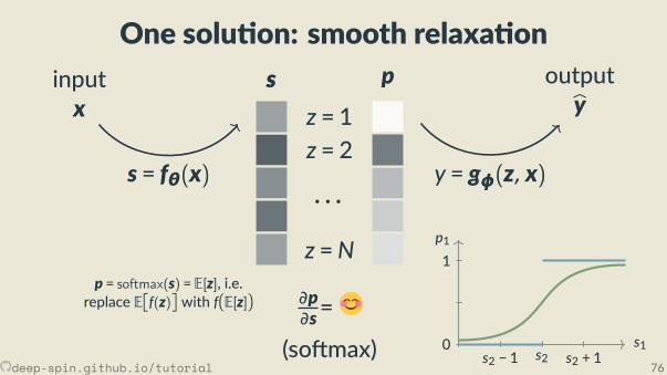
One solu on: smooth relaxa ons
z = 1z = 2
· · ·z =N
s
z
p
∂p∂s=
inputx
outputbys = fθ(x) y = gφ(z, x)
(so max)
p = softmax(s) = E[z], i.e.replace Ef(z)with fE[z]
p1
s10
1
s2 − 1 s2 s2 + 1deep-spin.github.io/tutorial 76

One solu on: smooth relaxa ons
z = 1z = 2
· · ·z =N
s
z
p
∂p∂s=
inputx
outputbys = fθ(x) y = gφ(z, x)
(so max)
p = softmax(s) = E[z], i.e.replace Ef(z)with fE[z]
p1
s10
1
s2 − 1 s2 s2 + 1deep-spin.github.io/tutorial 76
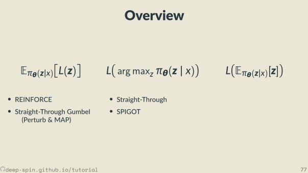
Overview
Eπθ(z|x)L(z)
• REINFORCE• Straight-Through Gumbel
(Perturb & MAP)
• SparseMAP
Largmaxz πθ(z | x)
• Straight-Through• SPIGOT
LEπθ(z|x)[z]
• Structured A n. Nets• SparseMAP
And more, a er the break!
deep-spin.github.io/tutorial 77
What is so max?O en de ned via pi =
exp si∑j exp sj
, but where does it come from?
p ∈ : probability distribu on over choicesExpected score under p: Ei∼p si = p⊤sargmax
maximizes expected score
Shannon entropy of p: H(p) = −∑
i pi log piso max maximizes expected score + entropy:
0.5 11.5
0.5 1 1.5
0.5
1
1.5
deep-spin.github.io/tutorial 78
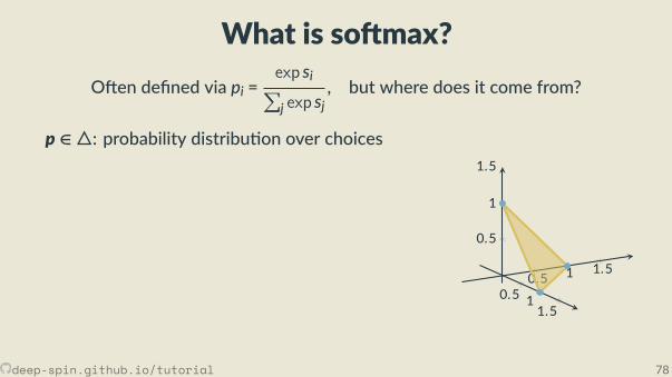
What is so max?O en de ned via pi =
exp si∑j exp sj
, but where does it come from?
p ∈ : probability distribu on over choices
Expected score under p: Ei∼p si = p⊤sargmax
maximizes expected score
Shannon entropy of p: H(p) = −∑
i pi log piso max maximizes expected score + entropy:
0.5 11.5
0.5 1 1.5
0.5
1
1.5
deep-spin.github.io/tutorial 78
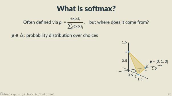
What is so max?O en de ned via pi =
exp si∑j exp sj
, but where does it come from?
p ∈ : probability distribu on over choices
Expected score under p: Ei∼p si = p⊤sargmax
maximizes expected score
Shannon entropy of p: H(p) = −∑
i pi log piso max maximizes expected score + entropy:
0.5 11.5
0.5 1 1.5
0.5
1
1.5
p = [0,1,0]
deep-spin.github.io/tutorial 78
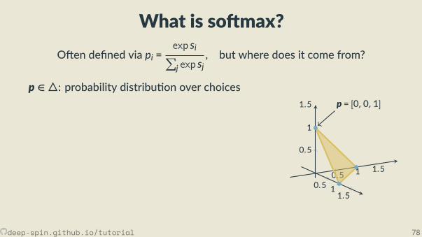
What is so max?O en de ned via pi =
exp si∑j exp sj
, but where does it come from?
p ∈ : probability distribu on over choices
Expected score under p: Ei∼p si = p⊤sargmax
maximizes expected score
Shannon entropy of p: H(p) = −∑
i pi log piso max maximizes expected score + entropy:
0.5 11.5
0.5 1 1.5
0.5
1
1.5 p = [0,0,1]
deep-spin.github.io/tutorial 78
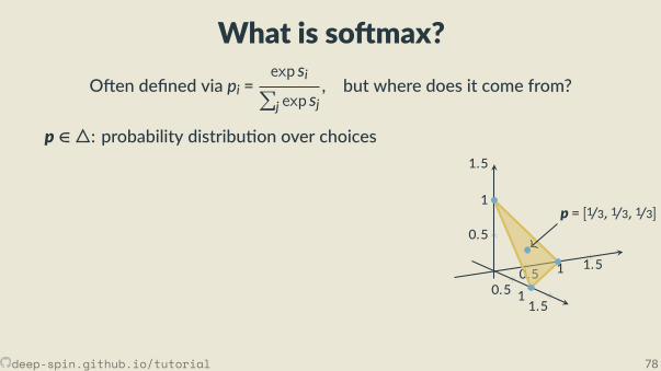
What is so max?O en de ned via pi =
exp si∑j exp sj
, but where does it come from?
p ∈ : probability distribu on over choices
Expected score under p: Ei∼p si = p⊤sargmax
maximizes expected score
Shannon entropy of p: H(p) = −∑
i pi log piso max maximizes expected score + entropy:
0.5 11.5
0.5 1 1.5
0.5
1
1.5
p = [1/3, 1/3, 1/3]
deep-spin.github.io/tutorial 78
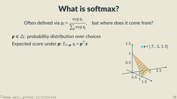
What is so max?O en de ned via pi =
exp si∑j exp sj
, but where does it come from?
p ∈ : probability distribu on over choicesExpected score under p: Ei∼p si = p⊤s
argmax
maximizes expected score
Shannon entropy of p: H(p) = −∑
i pi log piso max maximizes expected score + entropy:
0.5 11.5
0.5 1 1.5
0.5
1
1.5s = [.7, .1,1.5]
deep-spin.github.io/tutorial 78
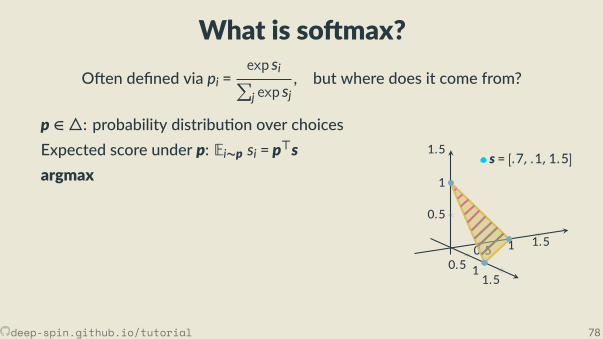
What is so max?O en de ned via pi =
exp si∑j exp sj
, but where does it come from?
p ∈ : probability distribu on over choicesExpected score under p: Ei∼p si = p⊤sargmax
maximizes expected scoreShannon entropy of p: H(p) = −
∑i pi log pi
so max maximizes expected score + entropy:
0.5 11.5
0.5 1 1.5
0.5
1
1.5s = [.7, .1,1.5]
deep-spin.github.io/tutorial 78
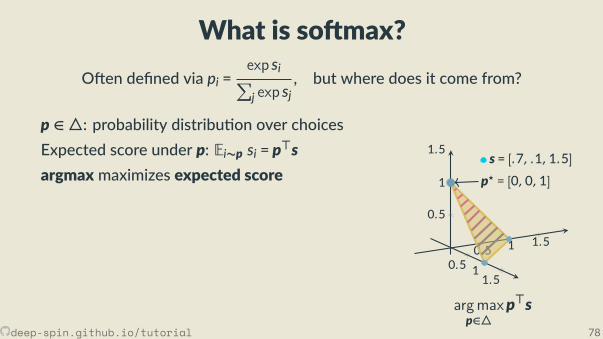
What is so max?O en de ned via pi =
exp si∑j exp sj
, but where does it come from?
p ∈ : probability distribu on over choicesExpected score under p: Ei∼p si = p⊤sargmax maximizes expected score
Shannon entropy of p: H(p) = −∑
i pi log piso max maximizes expected score + entropy:
0.5 11.5
0.5 1 1.5
0.5
1
1.5s = [.7, .1,1.5]
p⋆ = [0,0,1]
argmaxp∈
p⊤sdeep-spin.github.io/tutorial 78
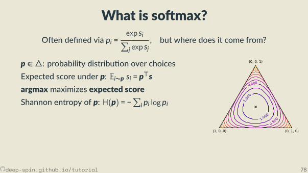
What is so max?O en de ned via pi =
exp si∑j exp sj
, but where does it come from?
p ∈ : probability distribu on over choicesExpected score under p: Ei∼p si = p⊤sargmax maximizes expected scoreShannon entropy of p: H(p) = −
∑i pi log pi
so max maximizes expected score + entropy:
(1, 0, 0) (0, 1, 0)
(0, 0, 1)
0.800
1.000
1.000
0.800
0.5 11.5
0.5 1 1.5
0.5
1
1.5s = [.7, .1,1.5]
p⋆ = [0,0,1]
argmaxp∈
p⊤s
deep-spin.github.io/tutorial 78
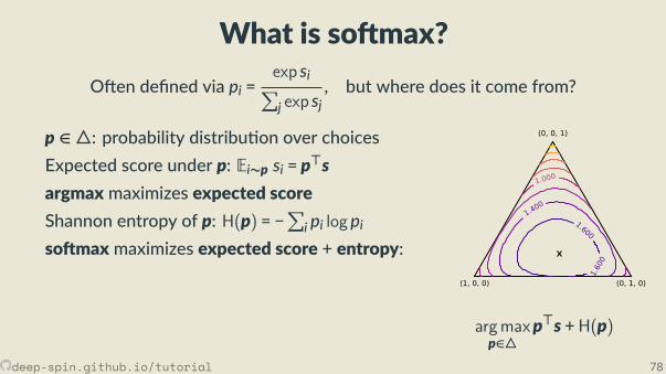
What is so max?O en de ned via pi =
exp si∑j exp sj
, but where does it come from?
p ∈ : probability distribu on over choicesExpected score under p: Ei∼p si = p⊤sargmax maximizes expected scoreShannon entropy of p: H(p) = −
∑i pi log pi
so max maximizes expected score + entropy:
(1, 0, 0) (0, 1, 0)
(0, 0, 1)
1.000
1.400
1.600
1.600
argmaxp∈
p⊤s +H(p)
0.5 11.5
0.5 1 1.5
0.5
1
1.5s = [.7, .1,1.5]
p⋆ = [0,0,1]
argmaxp∈
p⊤s
deep-spin.github.io/tutorial 78
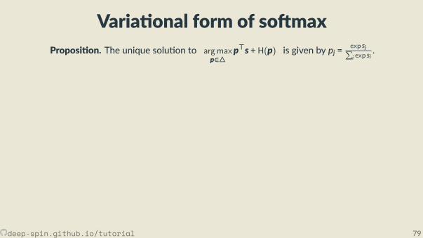
Varia onal form of so maxProposi on. The unique solu on to argmax
p∈p⊤s +H(p) is given by pj =
exp sj∑i exp si
.
Explicit form of the op miza on problem:
maximize∑
j pjsj − pj log pjsubject to p ≥ 0, p⊤1 = 1
Lagrangian:
L(p,ν, τ) = −∑
j pjsj − pj log pj − p⊤ν + τ(p⊤1 − 1)Op mality condi ons (KKT):
0 = ∇piL(p,ν, τ) = −si + logpi + 1 − νi + τ
p⊤ν = 0p ∈ ν ≥ 0
log pi = si + νi − (τ + 1)if pi = 0, r.h.s. must be −∞,thus pi > 0, so νi = 0.
pi = exp(si)/exp(τ+1) = exp(si)/Z
Must nd Z such that∑
j pj = 1.Answer: Z =∑
j exp(sj)
So, pi =exp(si)∑j exp(sj)
.
Classic result, e.g., [Boyd and Vandenberghe, 2004,Wainwright and Jordan, 2008]
deep-spin.github.io/tutorial 79
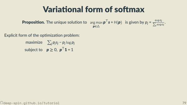
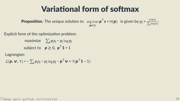
Varia onal form of so maxProposi on. The unique solu on to argmax
p∈p⊤s +H(p) is given by pj =
exp sj∑i exp si
.
Explicit form of the op miza on problem:
maximize∑
j pjsj − pj log pjsubject to p ≥ 0, p⊤1 = 1
Lagrangian:
L(p,ν, τ) = −∑
j pjsj − pj log pj − p⊤ν + τ(p⊤1 − 1)
Op mality condi ons (KKT):
0 = ∇piL(p,ν, τ) = −si + logpi + 1 − νi + τ
p⊤ν = 0p ∈ ν ≥ 0
log pi = si + νi − (τ + 1)if pi = 0, r.h.s. must be −∞,thus pi > 0, so νi = 0.
pi = exp(si)/exp(τ+1) = exp(si)/Z
Must nd Z such that∑
j pj = 1.Answer: Z =∑
j exp(sj)
So, pi =exp(si)∑j exp(sj)
.
Classic result, e.g., [Boyd and Vandenberghe, 2004,Wainwright and Jordan, 2008]
deep-spin.github.io/tutorial 79
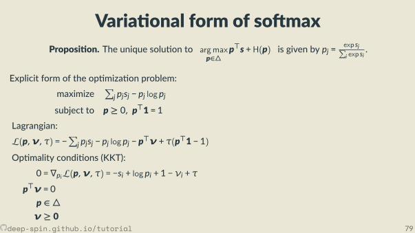
Varia onal form of so maxProposi on. The unique solu on to argmax
p∈p⊤s +H(p) is given by pj =
exp sj∑i exp si
.
Explicit form of the op miza on problem:
maximize∑
j pjsj − pj log pjsubject to p ≥ 0, p⊤1 = 1
Lagrangian:
L(p,ν, τ) = −∑
j pjsj − pj log pj − p⊤ν + τ(p⊤1 − 1)Op mality condi ons (KKT):
0 = ∇piL(p,ν, τ) = −si + logpi + 1 − νi + τ
p⊤ν = 0p ∈ ν ≥ 0
log pi = si + νi − (τ + 1)if pi = 0, r.h.s. must be −∞,thus pi > 0, so νi = 0.
pi = exp(si)/exp(τ+1) = exp(si)/Z
Must nd Z such that∑
j pj = 1.Answer: Z =∑
j exp(sj)
So, pi =exp(si)∑j exp(sj)
.
Classic result, e.g., [Boyd and Vandenberghe, 2004,Wainwright and Jordan, 2008]
deep-spin.github.io/tutorial 79
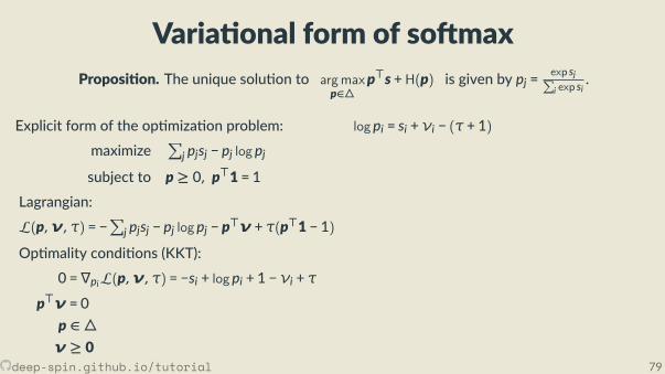
Varia onal form of so maxProposi on. The unique solu on to argmax
p∈p⊤s +H(p) is given by pj =
exp sj∑i exp si
.
Explicit form of the op miza on problem:
maximize∑
j pjsj − pj log pjsubject to p ≥ 0, p⊤1 = 1
Lagrangian:
L(p,ν, τ) = −∑
j pjsj − pj log pj − p⊤ν + τ(p⊤1 − 1)Op mality condi ons (KKT):
0 = ∇piL(p,ν, τ) = −si + logpi + 1 − νi + τ
p⊤ν = 0p ∈ ν ≥ 0
log pi = si + νi − (τ + 1)
if pi = 0, r.h.s. must be −∞,thus pi > 0, so νi = 0.
pi = exp(si)/exp(τ+1) = exp(si)/Z
Must nd Z such that∑
j pj = 1.Answer: Z =∑
j exp(sj)
So, pi =exp(si)∑j exp(sj)
.
Classic result, e.g., [Boyd and Vandenberghe, 2004,Wainwright and Jordan, 2008]
deep-spin.github.io/tutorial 79
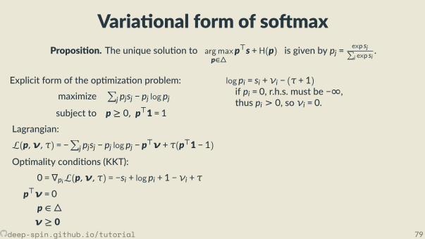
Varia onal form of so maxProposi on. The unique solu on to argmax
p∈p⊤s +H(p) is given by pj =
exp sj∑i exp si
.
Explicit form of the op miza on problem:
maximize∑
j pjsj − pj log pjsubject to p ≥ 0, p⊤1 = 1
Lagrangian:
L(p,ν, τ) = −∑
j pjsj − pj log pj − p⊤ν + τ(p⊤1 − 1)Op mality condi ons (KKT):
0 = ∇piL(p,ν, τ) = −si + logpi + 1 − νi + τ
p⊤ν = 0p ∈ ν ≥ 0
log pi = si + νi − (τ + 1)if pi = 0, r.h.s. must be −∞,thus pi > 0, so νi = 0.
pi = exp(si)/exp(τ+1) = exp(si)/Z
Must nd Z such that∑
j pj = 1.Answer: Z =∑
j exp(sj)
So, pi =exp(si)∑j exp(sj)
.
Classic result, e.g., [Boyd and Vandenberghe, 2004,Wainwright and Jordan, 2008]
deep-spin.github.io/tutorial 79
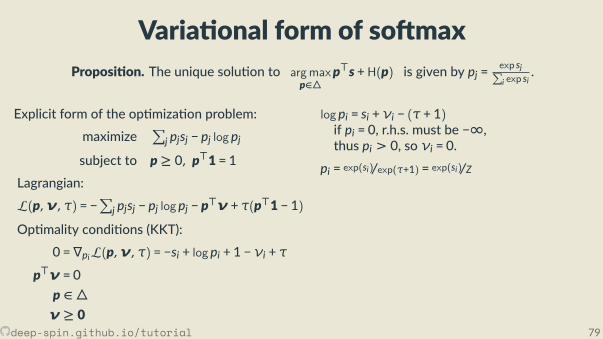
Varia onal form of so maxProposi on. The unique solu on to argmax
p∈p⊤s +H(p) is given by pj =
exp sj∑i exp si
.
Explicit form of the op miza on problem:
maximize∑
j pjsj − pj log pjsubject to p ≥ 0, p⊤1 = 1
Lagrangian:
L(p,ν, τ) = −∑
j pjsj − pj log pj − p⊤ν + τ(p⊤1 − 1)Op mality condi ons (KKT):
0 = ∇piL(p,ν, τ) = −si + logpi + 1 − νi + τ
p⊤ν = 0p ∈ ν ≥ 0
log pi = si + νi − (τ + 1)if pi = 0, r.h.s. must be −∞,thus pi > 0, so νi = 0.
pi = exp(si)/exp(τ+1) = exp(si)/Z
Must nd Z such that∑
j pj = 1.Answer: Z =∑
j exp(sj)
So, pi =exp(si)∑j exp(sj)
.
Classic result, e.g., [Boyd and Vandenberghe, 2004,Wainwright and Jordan, 2008]
deep-spin.github.io/tutorial 79
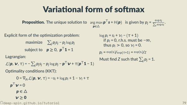
Varia onal form of so maxProposi on. The unique solu on to argmax
p∈p⊤s +H(p) is given by pj =
exp sj∑i exp si
.
Explicit form of the op miza on problem:
maximize∑
j pjsj − pj log pjsubject to p ≥ 0, p⊤1 = 1
Lagrangian:
L(p,ν, τ) = −∑
j pjsj − pj log pj − p⊤ν + τ(p⊤1 − 1)Op mality condi ons (KKT):
0 = ∇piL(p,ν, τ) = −si + logpi + 1 − νi + τ
p⊤ν = 0p ∈ ν ≥ 0
log pi = si + νi − (τ + 1)if pi = 0, r.h.s. must be −∞,thus pi > 0, so νi = 0.
pi = exp(si)/exp(τ+1) = exp(si)/Z
Must nd Z such that∑
j pj = 1.
Answer: Z =∑
j exp(sj)
So, pi =exp(si)∑j exp(sj)
.
Classic result, e.g., [Boyd and Vandenberghe, 2004,Wainwright and Jordan, 2008]
deep-spin.github.io/tutorial 79
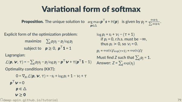
Varia onal form of so maxProposi on. The unique solu on to argmax
p∈p⊤s +H(p) is given by pj =
exp sj∑i exp si
.
Explicit form of the op miza on problem:
maximize∑
j pjsj − pj log pjsubject to p ≥ 0, p⊤1 = 1
Lagrangian:
L(p,ν, τ) = −∑
j pjsj − pj log pj − p⊤ν + τ(p⊤1 − 1)Op mality condi ons (KKT):
0 = ∇piL(p,ν, τ) = −si + logpi + 1 − νi + τ
p⊤ν = 0p ∈ ν ≥ 0
log pi = si + νi − (τ + 1)if pi = 0, r.h.s. must be −∞,thus pi > 0, so νi = 0.
pi = exp(si)/exp(τ+1) = exp(si)/Z
Must nd Z such that∑
j pj = 1.Answer: Z =∑
j exp(sj)
So, pi =exp(si)∑j exp(sj)
.
Classic result, e.g., [Boyd and Vandenberghe, 2004,Wainwright and Jordan, 2008]
deep-spin.github.io/tutorial 79
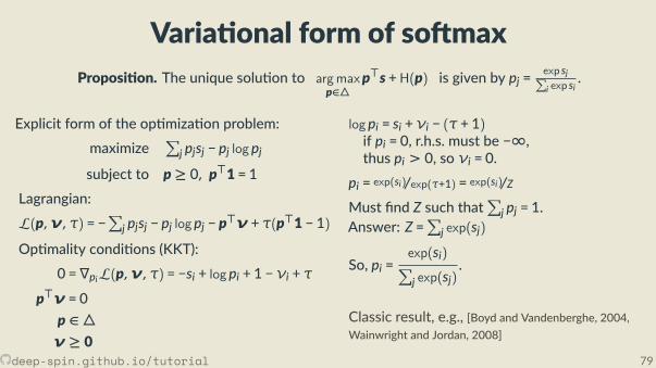
Varia onal form of so maxProposi on. The unique solu on to argmax
p∈p⊤s +H(p) is given by pj =
exp sj∑i exp si
.
Explicit form of the op miza on problem:
maximize∑
j pjsj − pj log pjsubject to p ≥ 0, p⊤1 = 1
Lagrangian:
L(p,ν, τ) = −∑
j pjsj − pj log pj − p⊤ν + τ(p⊤1 − 1)Op mality condi ons (KKT):
0 = ∇piL(p,ν, τ) = −si + logpi + 1 − νi + τ
p⊤ν = 0p ∈ ν ≥ 0
log pi = si + νi − (τ + 1)if pi = 0, r.h.s. must be −∞,thus pi > 0, so νi = 0.
pi = exp(si)/exp(τ+1) = exp(si)/Z
Must nd Z such that∑
j pj = 1.Answer: Z =∑
j exp(sj)
So, pi =exp(si)∑j exp(sj)
.
Classic result, e.g., [Boyd and Vandenberghe, 2004,Wainwright and Jordan, 2008]
deep-spin.github.io/tutorial 79

Generalizing so max: Smoothed argmaxespΩ(s) = argmax
p∈p⊤s −Ω(p)
argmax: Ω(p)=0
so max: Ω(p)=∑
j pj log pjsparsemax: Ω(p)= 1/2∥p∥22α-entmax: Ω(p)= 1/α(α−1)
∑j pαi
p1
s10
1
−1 0 1
[0,0,1]
[.3, .2, .5]
[.3,0, .7]
[Niculae and Blondel, 2017]
[Niculae and Blondel, 2017, Mar ns and Astudillo, 2016][Niculae and Blondel, 2017, Blondel et al., 2019][Niculae and Blondel, 2017, Mar ns and Kreutzer, 2017, Malaviya et al., 2018]
deep-spin.github.io/tutorial 80
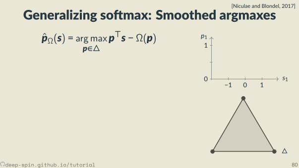
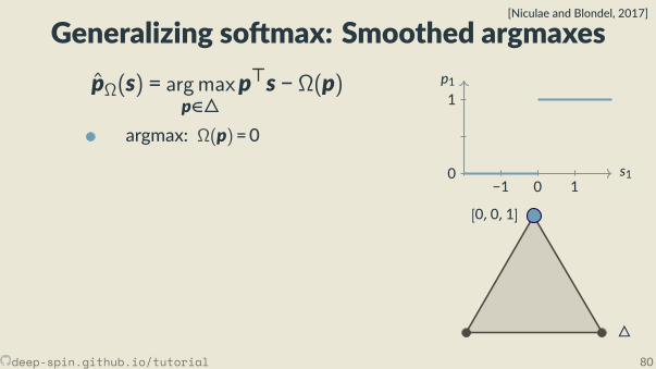
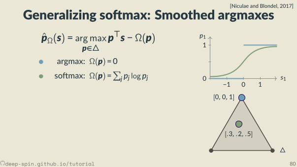
Generalizing so max: Smoothed argmaxespΩ(s) = argmax
p∈p⊤s −Ω(p)
argmax: Ω(p)=0
so max: Ω(p)=∑
j pj log pj
sparsemax: Ω(p)= 1/2∥p∥22α-entmax: Ω(p)= 1/α(α−1)
∑j pαi
p1
s10
1
−1 0 1
[0,0,1]
[.3, .2, .5]
[.3,0, .7]
[Niculae and Blondel, 2017]
[Niculae and Blondel, 2017, Mar ns and Astudillo, 2016][Niculae and Blondel, 2017, Blondel et al., 2019][Niculae and Blondel, 2017, Mar ns and Kreutzer, 2017, Malaviya et al., 2018]
deep-spin.github.io/tutorial 80
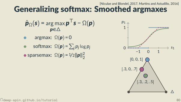
Generalizing so max: Smoothed argmaxespΩ(s) = argmax
p∈p⊤s −Ω(p)
argmax: Ω(p)=0
so max: Ω(p)=∑
j pj log pjsparsemax: Ω(p)= 1/2∥p∥22
α-entmax: Ω(p)= 1/α(α−1)∑
j pαi
p1
s10
1
−1 0 1
[0,0,1]
[.3, .2, .5]
[.3,0, .7]
[Niculae and Blondel, 2017]
[Niculae and Blondel, 2017, Mar ns and Astudillo, 2016]
[Niculae and Blondel, 2017, Blondel et al., 2019][Niculae and Blondel, 2017, Mar ns and Kreutzer, 2017, Malaviya et al., 2018]
deep-spin.github.io/tutorial 80
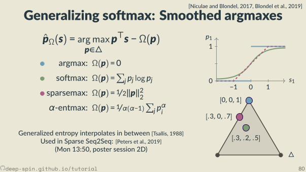
Generalizing so max: Smoothed argmaxespΩ(s) = argmax
p∈p⊤s −Ω(p)
argmax: Ω(p)=0
so max: Ω(p)=∑
j pj log pjsparsemax: Ω(p)= 1/2∥p∥22α-entmax: Ω(p)= 1/α(α−1)
∑j pαi
Generalized entropy interpolates in between [Tsallis, 1988]Used in Sparse Seq2Seq: [Peters et al., 2019]
(Mon 13:50, poster session 2D)
p1
s10
1
−1 0 1
[0,0,1]
[.3, .2, .5]
[.3,0, .7]
[Niculae and Blondel, 2017][Niculae and Blondel, 2017, Mar ns and Astudillo, 2016]
[Niculae and Blondel, 2017, Blondel et al., 2019]
[Niculae and Blondel, 2017, Mar ns and Kreutzer, 2017, Malaviya et al., 2018]
deep-spin.github.io/tutorial 80
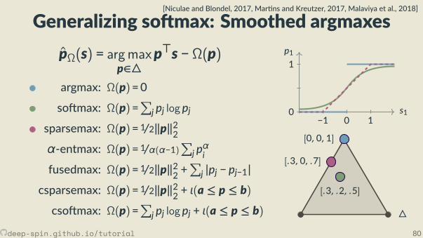
Generalizing so max: Smoothed argmaxespΩ(s) = argmax
p∈p⊤s −Ω(p)
argmax: Ω(p)=0
so max: Ω(p)=∑
j pj log pjsparsemax: Ω(p)= 1/2∥p∥22α-entmax: Ω(p)= 1/α(α−1)
∑j pαi
fusedmax: Ω(p)= 1/2∥p∥22 +∑
j |pj − pj−1|csparsemax: Ω(p)= 1/2∥p∥22 + ι(a ≤ p ≤ b)
cso max: Ω(p)=∑
j pj log pj + ι(a ≤ p ≤ b)
p1
s10
1
−1 0 1
[0,0,1]
[.3, .2, .5]
[.3,0, .7]
[Niculae and Blondel, 2017][Niculae and Blondel, 2017, Mar ns and Astudillo, 2016][Niculae and Blondel, 2017, Blondel et al., 2019]
[Niculae and Blondel, 2017, Mar ns and Kreutzer, 2017, Malaviya et al., 2018]
deep-spin.github.io/tutorial 80
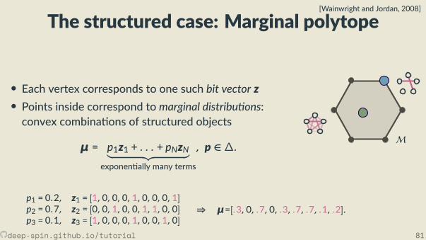
The structured case: Marginal polytope[Wainwright and Jordan, 2008]
• Each vertex corresponds to one such bit vector z• Points inside correspond to marginal distribu ons:convex combina ons of structured objects
μ = p1z1 + . . . + pNzN︸ ︷︷ ︸exponen ally many terms
, p ∈ ∆.
p1 = 0.2, z1 = [1,0,0,0,1,0,0,0,1]p2 = 0.7, z2 = [0,0,1,0,0,1,1,0,0]p3 = 0.1, z3 = [1,0,0,0,1,0,0,1,0]
⇒ μ=[.3,0, .7,0, .3, .7, .7, .1, .2].
M
deep-spin.github.io/tutorial 81
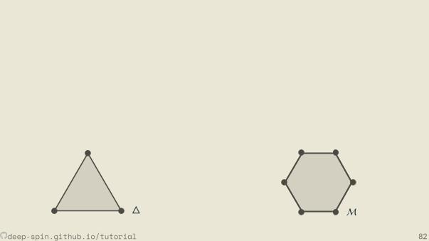
[Niculae et al., 2018a]
argmax argmaxp∈
p⊤s
so max argmaxp∈
p⊤s +H(p)
sparsemax argmaxp∈
p⊤s − 1/2∥p∥2
MAP argmaxμ∈M
μ⊤η
marginals argmaxμ∈M
μ⊤η + eH(μ)SparseMAP argmax
μ∈Mμ⊤η − 1/2∥μ∥2
M
Just like so max relaxes argmax,marginals relax MAP di eren ably!
Unlike argmax/so max, computa on is not obvious!
deep-spin.github.io/tutorial 82
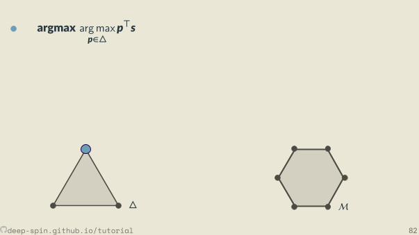
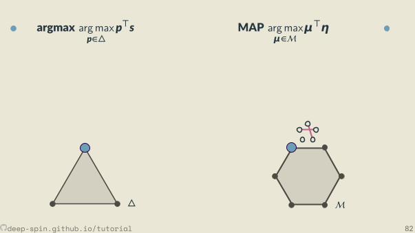
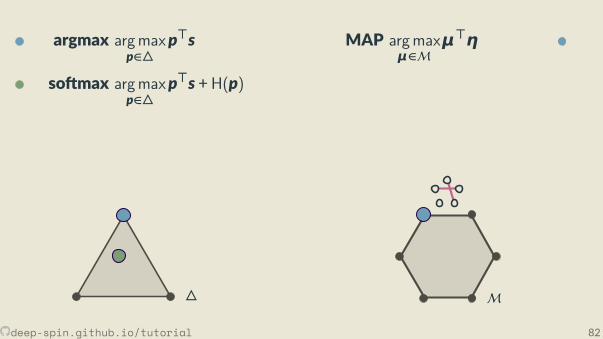
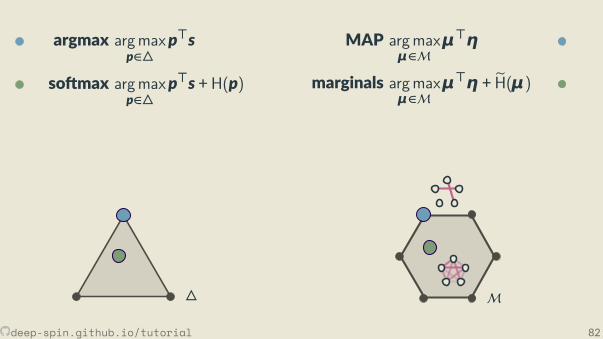
[Niculae et al., 2018a]
argmax argmaxp∈
p⊤s
so max argmaxp∈
p⊤s +H(p)
sparsemax argmaxp∈
p⊤s − 1/2∥p∥2
MAP argmaxμ∈M
μ⊤η
marginals argmaxμ∈M
μ⊤η + eH(μ)
SparseMAP argmaxμ∈M
μ⊤η − 1/2∥μ∥2
M
Just like so max relaxes argmax,marginals relax MAP di eren ably!
Unlike argmax/so max, computa on is not obvious!
deep-spin.github.io/tutorial 82
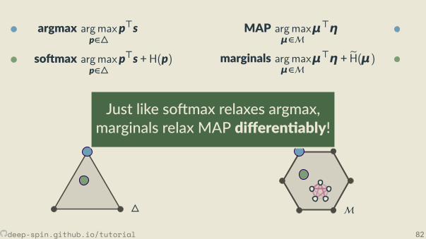
[Niculae et al., 2018a]
argmax argmaxp∈
p⊤s
so max argmaxp∈
p⊤s +H(p)
sparsemax argmaxp∈
p⊤s − 1/2∥p∥2
MAP argmaxμ∈M
μ⊤η
marginals argmaxμ∈M
μ⊤η + eH(μ)
SparseMAP argmaxμ∈M
μ⊤η − 1/2∥μ∥2
M
Just like so max relaxes argmax,marginals relax MAP di eren ably!
Unlike argmax/so max, computa on is not obvious!
deep-spin.github.io/tutorial 82
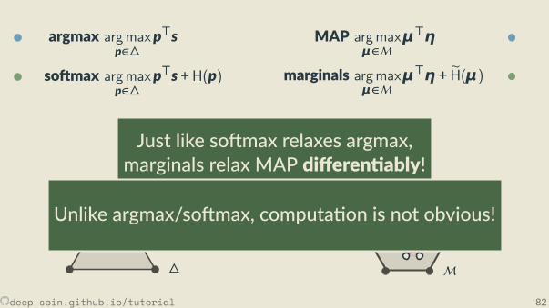
[Niculae et al., 2018a]
argmax argmaxp∈
p⊤s
so max argmaxp∈
p⊤s +H(p)
sparsemax argmaxp∈
p⊤s − 1/2∥p∥2
MAP argmaxμ∈M
μ⊤η
marginals argmaxμ∈M
μ⊤η + eH(μ)
SparseMAP argmaxμ∈M
μ⊤η − 1/2∥μ∥2
M
Just like so max relaxes argmax,marginals relax MAP di eren ably!
Unlike argmax/so max, computa on is not obvious!
deep-spin.github.io/tutorial 82
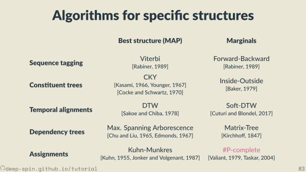
Algorithms for speci c structuresBest structure (MAP) Marginals
Sequence tagging Viterbi[Rabiner, 1989]
Forward-Backward[Rabiner, 1989]
Cons tuent treesCKY
[Kasami, 1966, Younger, 1967][Cocke and Schwartz, 1970]
Inside-Outside[Baker, 1979]
Temporal alignments DTW[Sakoe and Chiba, 1978]
So -DTW[Cuturi and Blondel, 2017]
Dependency trees Max. Spanning Arborescence[Chu and Liu, 1965, Edmonds, 1967]
Matrix-Tree[Kirchho , 1847]
Assignments Kuhn-Munkres[Kuhn, 1955, Jonker and Volgenant, 1987]
#P-complete[Valiant, 1979, Taskar, 2004]
deep-spin.github.io/tutorial 83
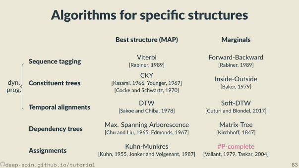
Algorithms for speci c structuresBest structure (MAP) Marginals
Sequence tagging Viterbi[Rabiner, 1989]
Forward-Backward[Rabiner, 1989]
Cons tuent treesCKY
[Kasami, 1966, Younger, 1967][Cocke and Schwartz, 1970]
Inside-Outside[Baker, 1979]
Temporal alignments DTW[Sakoe and Chiba, 1978]
So -DTW[Cuturi and Blondel, 2017]
Dependency trees Max. Spanning Arborescence[Chu and Liu, 1965, Edmonds, 1967]
Matrix-Tree[Kirchho , 1847]
Assignments Kuhn-Munkres[Kuhn, 1955, Jonker and Volgenant, 1987]
#P-complete[Valiant, 1979, Taskar, 2004]
dyn.prog.
deep-spin.github.io/tutorial 83
Deriva ves of marginals 1: DPDynamic programming: marginals by Forward-Backward, Inside-Outside, etc.
• Alg. consists of di eren able ops: PyTorch autograd can handle it! (v. bad idea)• Be er book-keeping: Li and Eisner [2009], Mensch and Blondel [2018]• With circular dependencies, this breaks! Can get an approxima on Stoyanov et al. [2011]Marginals in a sequence tagging model.1 input: d tags, n tokens, ηU ∈ Rn×d,ηV ∈ Rd×d2 ini alize α1 = 0,βn = 03 for i ∈ 2, . . . ,n do # forward log-probabili es4 αi,k = log
∑k′ expαi−1,k′ + (ηU)i,k + (ηV)k′,k
for all k
5 for i ∈ n − 1, . . . ,1 do # backward log-probabili es6 βi,k = log∑
k′ expβi+1,k′ + (ηU)i+1,k′ + (ηV)k,k′
for all k
7 Z =∑
k expαn,k # par on func on8 return μ = exp
α +β − logZ
# marginals
(ηU)1,NN
(ηU)1,VB
(ηU)1,PR
(ηU)2,NN
(ηU)2,VB
(ηU)2,PR
ηV
(ηU)n,NN
(ηU)n,VB
(ηU)n,PR
deep-spin.github.io/tutorial 84
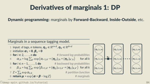
Deriva ves of marginals 1: DPDynamic programming: marginals by Forward-Backward, Inside-Outside, etc.
• Alg. consists of di eren able ops: PyTorch autograd can handle it! (v. bad idea)• Be er book-keeping: Li and Eisner [2009], Mensch and Blondel [2018]• With circular dependencies, this breaks! Can get an approxima on Stoyanov et al. [2011]
Marginals in a sequence tagging model.1 input: d tags, n tokens, ηU ∈ Rn×d,ηV ∈ Rd×d2 ini alize α1 = 0,βn = 03 for i ∈ 2, . . . ,n do # forward log-probabili es4 αi,k = log
∑k′ expαi−1,k′ + (ηU)i,k + (ηV)k′,k
for all k
5 for i ∈ n − 1, . . . ,1 do # backward log-probabili es6 βi,k = log∑
k′ expβi+1,k′ + (ηU)i+1,k′ + (ηV)k,k′
for all k
7 Z =∑
k expαn,k # par on func on8 return μ = exp
α +β − logZ
# marginals
(ηU)1,NN
(ηU)1,VB
(ηU)1,PR
(ηU)2,NN
(ηU)2,VB
(ηU)2,PR
ηV
(ηU)n,NN
(ηU)n,VB
(ηU)n,PR
deep-spin.github.io/tutorial 84
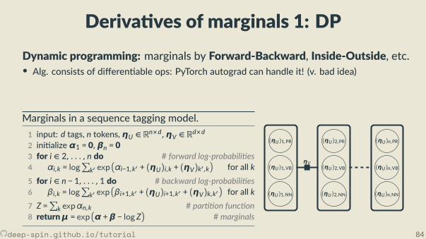
Deriva ves of marginals 1: DPDynamic programming: marginals by Forward-Backward, Inside-Outside, etc.• Alg. consists of di eren able ops: PyTorch autograd can handle it! (v. bad idea)
• Be er book-keeping: Li and Eisner [2009], Mensch and Blondel [2018]• With circular dependencies, this breaks! Can get an approxima on Stoyanov et al. [2011]
Marginals in a sequence tagging model.1 input: d tags, n tokens, ηU ∈ Rn×d,ηV ∈ Rd×d2 ini alize α1 = 0,βn = 03 for i ∈ 2, . . . ,n do # forward log-probabili es4 αi,k = log
∑k′ expαi−1,k′ + (ηU)i,k + (ηV)k′,k
for all k
5 for i ∈ n − 1, . . . ,1 do # backward log-probabili es6 βi,k = log∑
k′ expβi+1,k′ + (ηU)i+1,k′ + (ηV)k,k′
for all k
7 Z =∑
k expαn,k # par on func on8 return μ = exp
α +β − logZ
# marginals
(ηU)1,NN
(ηU)1,VB
(ηU)1,PR
(ηU)2,NN
(ηU)2,VB
(ηU)2,PR
ηV
(ηU)n,NN
(ηU)n,VB
(ηU)n,PR
deep-spin.github.io/tutorial 84
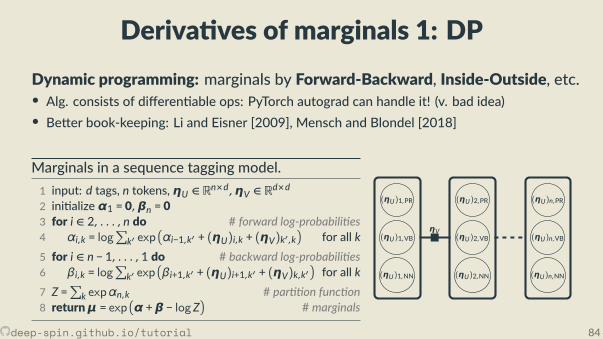
Deriva ves of marginals 1: DPDynamic programming: marginals by Forward-Backward, Inside-Outside, etc.• Alg. consists of di eren able ops: PyTorch autograd can handle it! (v. bad idea)• Be er book-keeping: Li and Eisner [2009], Mensch and Blondel [2018]
• With circular dependencies, this breaks! Can get an approxima on Stoyanov et al. [2011]
Marginals in a sequence tagging model.1 input: d tags, n tokens, ηU ∈ Rn×d,ηV ∈ Rd×d2 ini alize α1 = 0,βn = 03 for i ∈ 2, . . . ,n do # forward log-probabili es4 αi,k = log
∑k′ expαi−1,k′ + (ηU)i,k + (ηV)k′,k
for all k
5 for i ∈ n − 1, . . . ,1 do # backward log-probabili es6 βi,k = log∑
k′ expβi+1,k′ + (ηU)i+1,k′ + (ηV)k,k′
for all k
7 Z =∑
k expαn,k # par on func on8 return μ = exp
α +β − logZ
# marginals
(ηU)1,NN
(ηU)1,VB
(ηU)1,PR
(ηU)2,NN
(ηU)2,VB
(ηU)2,PR
ηV
(ηU)n,NN
(ηU)n,VB
(ηU)n,PR
deep-spin.github.io/tutorial 84
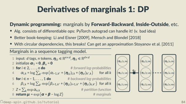
Deriva ves of marginals 1: DPDynamic programming: marginals by Forward-Backward, Inside-Outside, etc.• Alg. consists of di eren able ops: PyTorch autograd can handle it! (v. bad idea)• Be er book-keeping: Li and Eisner [2009], Mensch and Blondel [2018]• With circular dependencies, this breaks! Can get an approxima on Stoyanov et al. [2011]Marginals in a sequence tagging model.1 input: d tags, n tokens, ηU ∈ Rn×d,ηV ∈ Rd×d2 ini alize α1 = 0,βn = 03 for i ∈ 2, . . . ,n do # forward log-probabili es4 αi,k = log
∑k′ expαi−1,k′ + (ηU)i,k + (ηV)k′,k
for all k
5 for i ∈ n − 1, . . . ,1 do # backward log-probabili es6 βi,k = log∑
k′ expβi+1,k′ + (ηU)i+1,k′ + (ηV)k,k′
for all k
7 Z =∑
k expαn,k # par on func on8 return μ = exp
α +β − logZ
# marginals
(ηU)1,NN
(ηU)1,VB
(ηU)1,PR
(ηU)2,NN
(ηU)2,VB
(ηU)2,PR
ηV
(ηU)n,NN
(ηU)n,VB
(ηU)n,PR
deep-spin.github.io/tutorial 84
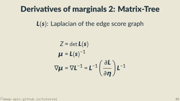
Deriva ves of marginals 2: Matrix-Tree
L(s): Laplacian of the edge score graph
Z = detL(s)μ = L(s)−1
∇μ = ∇L−1 = L−1∂L∂η
L−1
deep-spin.github.io/tutorial 85
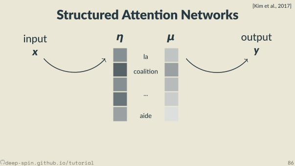
Structured A en on Networks
la
coali on
...
aide
η μinputx
outputy
CRF marginals (from forward–backward) give a en on weights ∈ (0,1)Similar idea for projec ve dependency trees with inside–outside
and non-projec ve with the Matrix-Tree theorem [Liu and Lapata, 2018].
[Kim et al., 2017]
deep-spin.github.io/tutorial 86
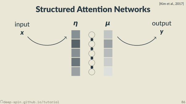
Structured A en on Networksη μinput
xoutput
y
CRF marginals (from forward–backward) give a en on weights ∈ (0,1)Similar idea for projec ve dependency trees with inside–outside
and non-projec ve with the Matrix-Tree theorem [Liu and Lapata, 2018].
[Kim et al., 2017]
deep-spin.github.io/tutorial 86
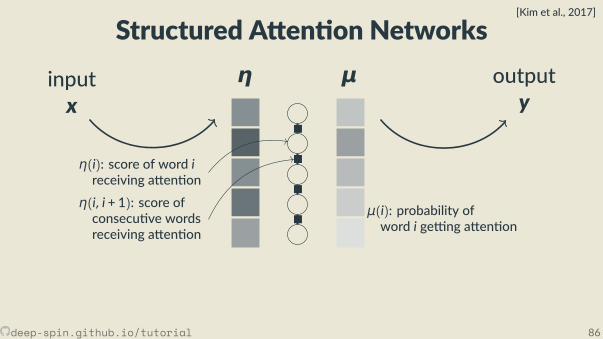
Structured A en on Networksη μinput
xoutput
y
η(i): score of word ireceiving a en on
η(i, i + 1): score ofconsecu ve wordsreceiving a en on
μ(i): probability ofword i ge ng a en on
CRF marginals (from forward–backward) give a en on weights ∈ (0,1)Similar idea for projec ve dependency trees with inside–outside
and non-projec ve with the Matrix-Tree theorem [Liu and Lapata, 2018].
[Kim et al., 2017]
deep-spin.github.io/tutorial 86
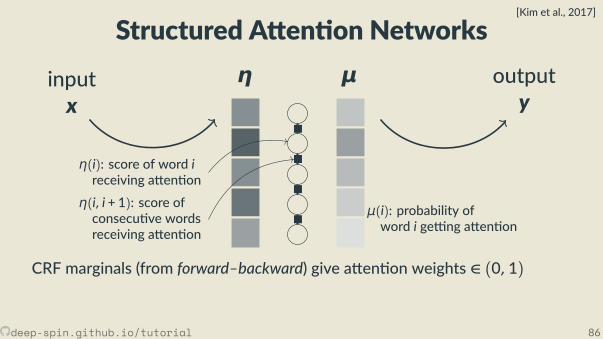
Structured A en on Networksη μinput
xoutput
y
η(i): score of word ireceiving a en on
η(i, i + 1): score ofconsecu ve wordsreceiving a en on
μ(i): probability ofword i ge ng a en on
CRF marginals (from forward–backward) give a en on weights ∈ (0,1)
Similar idea for projec ve dependency trees with inside–outside
and non-projec ve with the Matrix-Tree theorem [Liu and Lapata, 2018].
[Kim et al., 2017]
deep-spin.github.io/tutorial 86
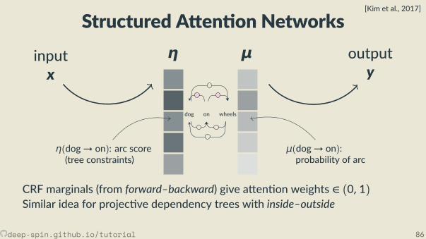
Structured A en on Networksη μinput
xoutput
y
dog on wheels
η(dog→ on): arc score(tree constraints)
μ(dog→ on):probability of arc
CRF marginals (from forward–backward) give a en on weights ∈ (0,1)Similar idea for projec ve dependency trees with inside–outside
and non-projec ve with the Matrix-Tree theorem [Liu and Lapata, 2018].
[Kim et al., 2017]
deep-spin.github.io/tutorial 86
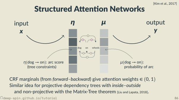
Structured A en on Networksη μinput
xoutput
y
dog on wheels
η(dog→ on): arc score(tree constraints)
μ(dog→ on):probability of arc
CRF marginals (from forward–backward) give a en on weights ∈ (0,1)Similar idea for projec ve dependency trees with inside–outsideand non-projec ve with the Matrix-Tree theorem [Liu and Lapata, 2018].
[Kim et al., 2017]
deep-spin.github.io/tutorial 86
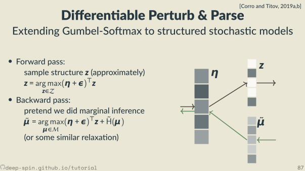
Di eren able Perturb & ParseExtending Gumbel-So max to structured stochas c models
• Forward pass:sample structure z (approximately)z = argmax
z∈Z(η + ε)⊤z
• Backward pass:pretend we did marginal inferenceμ = argmax
μ∈M(η + ε)⊤z + H(μ)
(or some similar relaxa on)
ηz
μ
[Corro and Titov, 2019a,b]
deep-spin.github.io/tutorial 87
Back-propaga ng through marginalsPros:
• Familiar algorithms for NLPers,• (Structured A en on Networks:) All computa ons exact.
Cons:
• (Structured A en on Networks:) forward pass marginals are dense;( xed by Perturb & MAP, at cost of rough approxima on)
• E cient & numerically stable back-propaga on through DPs is tricky;(somewhat alleviated by Mensch and Blondel [2018])
• Not applicable when marginals are unavailable.• Case-by-case algorithms required, can get tedious.
deep-spin.github.io/tutorial 88
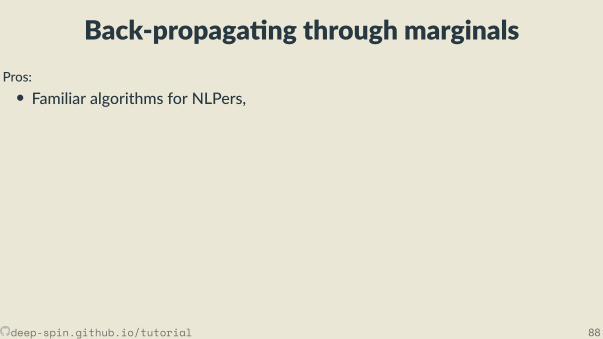
Back-propaga ng through marginalsPros:• Familiar algorithms for NLPers,
• (Structured A en on Networks:) All computa ons exact.Cons:
• (Structured A en on Networks:) forward pass marginals are dense;( xed by Perturb & MAP, at cost of rough approxima on)
• E cient & numerically stable back-propaga on through DPs is tricky;(somewhat alleviated by Mensch and Blondel [2018])
• Not applicable when marginals are unavailable.• Case-by-case algorithms required, can get tedious.
deep-spin.github.io/tutorial 88
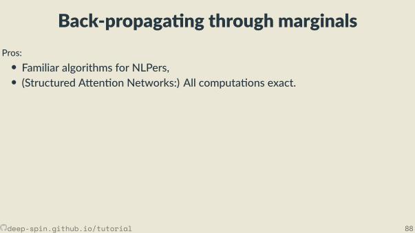
Back-propaga ng through marginalsPros:• Familiar algorithms for NLPers,• (Structured A en on Networks:) All computa ons exact.
Cons:
• (Structured A en on Networks:) forward pass marginals are dense;( xed by Perturb & MAP, at cost of rough approxima on)
• E cient & numerically stable back-propaga on through DPs is tricky;(somewhat alleviated by Mensch and Blondel [2018])
• Not applicable when marginals are unavailable.• Case-by-case algorithms required, can get tedious.
deep-spin.github.io/tutorial 88
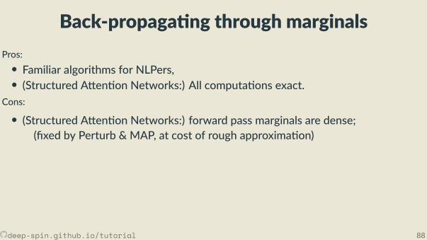
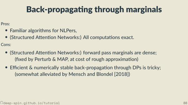
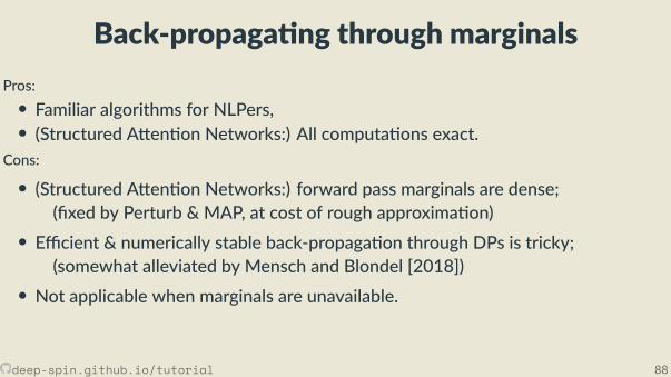
Back-propaga ng through marginalsPros:• Familiar algorithms for NLPers,• (Structured A en on Networks:) All computa ons exact.
Cons:
• (Structured A en on Networks:) forward pass marginals are dense;( xed by Perturb & MAP, at cost of rough approxima on)
• E cient & numerically stable back-propaga on through DPs is tricky;(somewhat alleviated by Mensch and Blondel [2018])
• Not applicable when marginals are unavailable.
• Case-by-case algorithms required, can get tedious.
deep-spin.github.io/tutorial 88

Back-propaga ng through marginalsPros:• Familiar algorithms for NLPers,• (Structured A en on Networks:) All computa ons exact.
Cons:
• (Structured A en on Networks:) forward pass marginals are dense;( xed by Perturb & MAP, at cost of rough approxima on)
• E cient & numerically stable back-propaga on through DPs is tricky;(somewhat alleviated by Mensch and Blondel [2018])
• Not applicable when marginals are unavailable.• Case-by-case algorithms required, can get tedious.deep-spin.github.io/tutorial 88
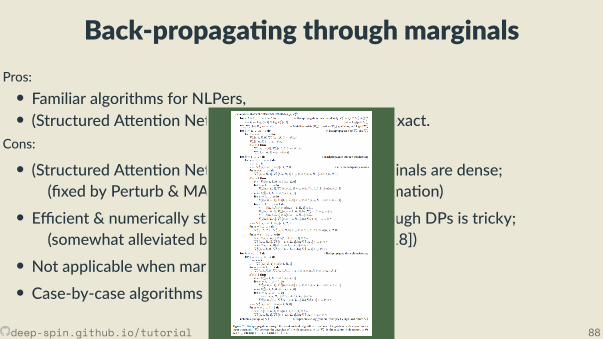
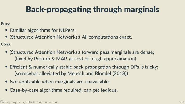
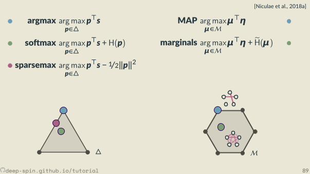
[Niculae et al., 2018a]
argmax argmaxp∈
p⊤s
so max argmaxp∈
p⊤s +H(p)
sparsemax argmaxp∈
p⊤s − 1/2∥p∥2
MAP argmaxμ∈M
μ⊤η
marginals argmaxμ∈M
μ⊤η + eH(μ)
SparseMAP argmaxμ∈M
μ⊤η − 1/2∥μ∥2
M
Just like so max relaxes argmax,marginals relax MAP di eren ably!
Unlike argmax/so max, computa on is not obvious!
deep-spin.github.io/tutorial 89
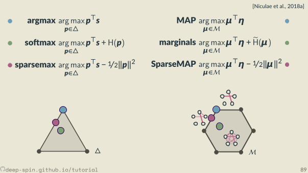
[Niculae et al., 2018a]
argmax argmaxp∈
p⊤s
so max argmaxp∈
p⊤s +H(p)
sparsemax argmaxp∈
p⊤s − 1/2∥p∥2
MAP argmaxμ∈M
μ⊤η
marginals argmaxμ∈M
μ⊤η + eH(μ)SparseMAP argmax
μ∈Mμ⊤η − 1/2∥μ∥2
M
Just like so max relaxes argmax,marginals relax MAP di eren ably!
Unlike argmax/so max, computa on is not obvious!
deep-spin.github.io/tutorial 89
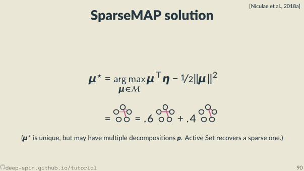
SparseMAP solu on[Niculae et al., 2018a]
μ⋆ = argmaxμ∈M
μ⊤η − 1/2∥μ∥2
= = .6 + .4(μ⋆ is unique, but may have mul ple decomposi ons p. Ac ve Set recovers a sparse one.)
deep-spin.github.io/tutorial 90
Algorithms for SparseMAPμ⋆ = argmax
μ∈Mμ⊤η − 1/2∥μ∥2
Condi onal Gradient[Frank and Wolfe, 1956, Lacoste-Julien and Jaggi, 2015]
• select a new corner ofM• update the (sparse) coe cients of p
• Update rules: vanilla, away-step, pairwise• Quadra c objec ve: Ac ve Seta.k.a. Min-Norm Point, [Wolfe, 1976][Mar ns et al., 2015, Nocedal and Wright, 1999,
Vinyes and Obozinski, 2017]
Backward pass
∂μ∂η is sparse
compu ng∂μ∂η
⊤dy
takes O(dim(μ) nnz(p⋆))
quadra c objec velinear constraints(alas, exponen ally many!)
argmaxμ∈M
μ⊤ (η −μ(t−1))︸ ︷︷ ︸eηAc ve Set achieves
nite & linear convergence!
Completely modular: just add MAP
deep-spin.github.io/tutorial 91
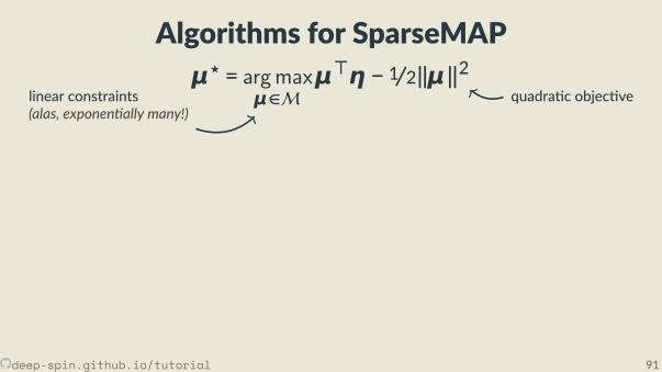
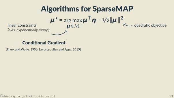
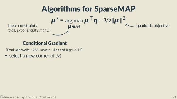
Algorithms for SparseMAPμ⋆ = argmax
μ∈Mμ⊤η − 1/2∥μ∥2
Condi onal Gradient[Frank and Wolfe, 1956, Lacoste-Julien and Jaggi, 2015]
• select a new corner ofM
• update the (sparse) coe cients of p
• Update rules: vanilla, away-step, pairwise• Quadra c objec ve: Ac ve Seta.k.a. Min-Norm Point, [Wolfe, 1976][Mar ns et al., 2015, Nocedal and Wright, 1999,
Vinyes and Obozinski, 2017]
Backward pass
∂μ∂η is sparse
compu ng∂μ∂η
⊤dy
takes O(dim(μ) nnz(p⋆))
quadra c objec velinear constraints(alas, exponen ally many!)
argmaxμ∈M
μ⊤ (η −μ(t−1))︸ ︷︷ ︸eηAc ve Set achieves
nite & linear convergence!
Completely modular: just add MAP
deep-spin.github.io/tutorial 91
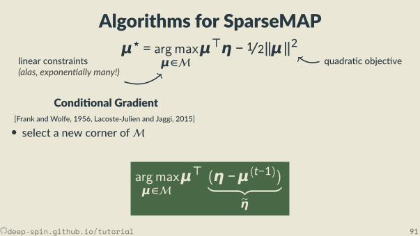
Algorithms for SparseMAPμ⋆ = argmax
μ∈Mμ⊤η − 1/2∥μ∥2
Condi onal Gradient[Frank and Wolfe, 1956, Lacoste-Julien and Jaggi, 2015]
• select a new corner ofM
• update the (sparse) coe cients of p
• Update rules: vanilla, away-step, pairwise• Quadra c objec ve: Ac ve Seta.k.a. Min-Norm Point, [Wolfe, 1976][Mar ns et al., 2015, Nocedal and Wright, 1999,
Vinyes and Obozinski, 2017]
Backward pass
∂μ∂η is sparse
compu ng∂μ∂η
⊤dy
takes O(dim(μ) nnz(p⋆))
quadra c objec velinear constraints(alas, exponen ally many!)
argmaxμ∈M
μ⊤ (η −μ(t−1))︸ ︷︷ ︸eη
Ac ve Set achievesnite & linear convergence!
Completely modular: just add MAP
deep-spin.github.io/tutorial 91
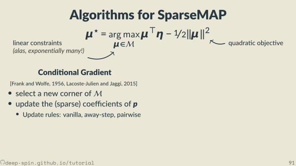
Algorithms for SparseMAPμ⋆ = argmax
μ∈Mμ⊤η − 1/2∥μ∥2
Condi onal Gradient[Frank and Wolfe, 1956, Lacoste-Julien and Jaggi, 2015]
• select a new corner ofM• update the (sparse) coe cients of p• Update rules: vanilla, away-step, pairwise
• Quadra c objec ve: Ac ve Seta.k.a. Min-Norm Point, [Wolfe, 1976][Mar ns et al., 2015, Nocedal and Wright, 1999,
Vinyes and Obozinski, 2017]
Backward pass
∂μ∂η is sparse
compu ng∂μ∂η
⊤dy
takes O(dim(μ) nnz(p⋆))
quadra c objec velinear constraints(alas, exponen ally many!)
argmaxμ∈M
μ⊤ (η −μ(t−1))︸ ︷︷ ︸eηAc ve Set achieves
nite & linear convergence!
Completely modular: just add MAP
deep-spin.github.io/tutorial 91
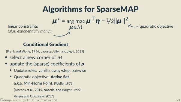
Algorithms for SparseMAPμ⋆ = argmax
μ∈Mμ⊤η − 1/2∥μ∥2
Condi onal Gradient[Frank and Wolfe, 1956, Lacoste-Julien and Jaggi, 2015]
• select a new corner ofM• update the (sparse) coe cients of p• Update rules: vanilla, away-step, pairwise• Quadra c objec ve: Ac ve Seta.k.a. Min-Norm Point, [Wolfe, 1976][Mar ns et al., 2015, Nocedal and Wright, 1999,
Vinyes and Obozinski, 2017]
Backward pass
∂μ∂η is sparse
compu ng∂μ∂η
⊤dy
takes O(dim(μ) nnz(p⋆))
quadra c objec velinear constraints(alas, exponen ally many!)
argmaxμ∈M
μ⊤ (η −μ(t−1))︸ ︷︷ ︸eηAc ve Set achieves
nite & linear convergence!
Completely modular: just add MAP
deep-spin.github.io/tutorial 91
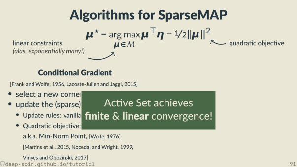
Algorithms for SparseMAPμ⋆ = argmax
μ∈Mμ⊤η − 1/2∥μ∥2
Condi onal Gradient[Frank and Wolfe, 1956, Lacoste-Julien and Jaggi, 2015]
• select a new corner ofM• update the (sparse) coe cients of p• Update rules: vanilla, away-step, pairwise• Quadra c objec ve: Ac ve Seta.k.a. Min-Norm Point, [Wolfe, 1976][Mar ns et al., 2015, Nocedal and Wright, 1999,
Vinyes and Obozinski, 2017]
Backward pass
∂μ∂η is sparse
compu ng∂μ∂η
⊤dy
takes O(dim(μ) nnz(p⋆))
quadra c objec velinear constraints(alas, exponen ally many!)
argmaxμ∈M
μ⊤ (η −μ(t−1))︸ ︷︷ ︸eη
Ac ve Set achievesnite & linear convergence!
Completely modular: just add MAP
deep-spin.github.io/tutorial 91
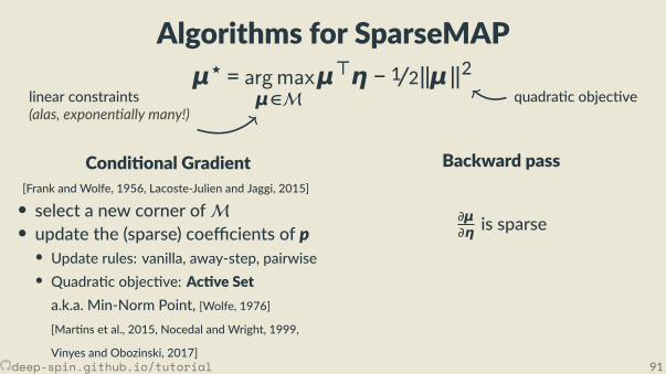
Algorithms for SparseMAPμ⋆ = argmax
μ∈Mμ⊤η − 1/2∥μ∥2
Condi onal Gradient[Frank and Wolfe, 1956, Lacoste-Julien and Jaggi, 2015]
• select a new corner ofM• update the (sparse) coe cients of p• Update rules: vanilla, away-step, pairwise• Quadra c objec ve: Ac ve Seta.k.a. Min-Norm Point, [Wolfe, 1976][Mar ns et al., 2015, Nocedal and Wright, 1999,
Vinyes and Obozinski, 2017]
Backward pass
∂μ∂η is sparse
compu ng∂μ∂η
⊤dy
takes O(dim(μ) nnz(p⋆))
quadra c objec velinear constraints(alas, exponen ally many!)
argmaxμ∈M
μ⊤ (η −μ(t−1))︸ ︷︷ ︸eηAc ve Set achieves
nite & linear convergence!
Completely modular: just add MAP
deep-spin.github.io/tutorial 91
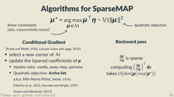
Algorithms for SparseMAPμ⋆ = argmax
μ∈Mμ⊤η − 1/2∥μ∥2
Condi onal Gradient[Frank and Wolfe, 1956, Lacoste-Julien and Jaggi, 2015]
• select a new corner ofM• update the (sparse) coe cients of p• Update rules: vanilla, away-step, pairwise• Quadra c objec ve: Ac ve Seta.k.a. Min-Norm Point, [Wolfe, 1976][Mar ns et al., 2015, Nocedal and Wright, 1999,
Vinyes and Obozinski, 2017]
Backward pass
∂μ∂η is sparse
compu ng∂μ∂η
⊤dy
takes O(dim(μ) nnz(p⋆))
quadra c objec velinear constraints(alas, exponen ally many!)
argmaxμ∈M
μ⊤ (η −μ(t−1))︸ ︷︷ ︸eηAc ve Set achieves
nite & linear convergence!
Completely modular: just add MAP
deep-spin.github.io/tutorial 91
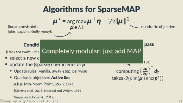
Algorithms for SparseMAPμ⋆ = argmax
μ∈Mμ⊤η − 1/2∥μ∥2
Condi onal Gradient[Frank and Wolfe, 1956, Lacoste-Julien and Jaggi, 2015]
• select a new corner ofM• update the (sparse) coe cients of p• Update rules: vanilla, away-step, pairwise• Quadra c objec ve: Ac ve Seta.k.a. Min-Norm Point, [Wolfe, 1976][Mar ns et al., 2015, Nocedal and Wright, 1999,
Vinyes and Obozinski, 2017]
Backward pass
∂μ∂η is sparse
compu ng∂μ∂η
⊤dy
takes O(dim(μ) nnz(p⋆))
quadra c objec velinear constraints(alas, exponen ally many!)
argmaxμ∈M
μ⊤ (η −μ(t−1))︸ ︷︷ ︸eηAc ve Set achieves
nite & linear convergence!
Completely modular: just add MAP
deep-spin.github.io/tutorial 91
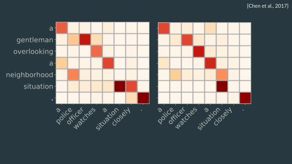
[Chen et al., 2017]
a
gentleman
overlooking
a
neighborhood
situation
.
a
police
officer
watches a
situation
closely . a
police
officer
watches a
situation
closely .
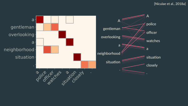
[Niculae et al., 2018a]
a
police
officer
watches a
situation
closely .
a
gentleman
overlooking
a
neighborhood
situation
.
A
gentleman
overlooking
a
neighborhood
situa on
.
A
police
o cer
watches
a
situa on
closely
.
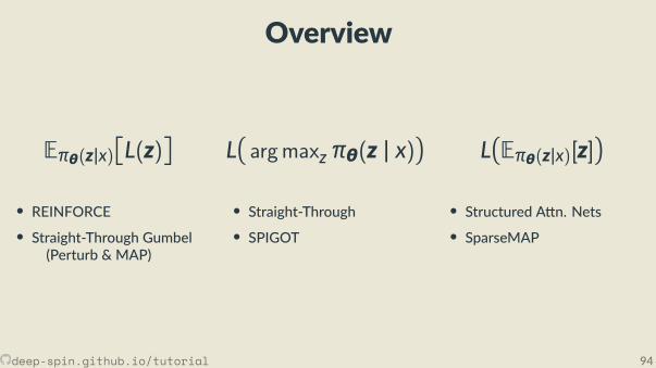
Overview
Eπθ(z|x)L(z)
• REINFORCE• Straight-Through Gumbel
(Perturb & MAP)
• SparseMAP
Largmaxz πθ(z | x)
• Straight-Through• SPIGOT
LEπθ(z|x)[z]
• Structured A n. Nets• SparseMAP
And more, a er the break!
deep-spin.github.io/tutorial 94
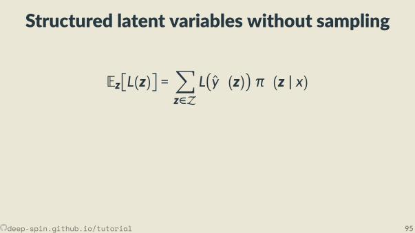
Structured latent variables without sampling
EzL(z)=∑z∈Z
Ly
φ
(z)π
θ
(z | x)
How to de ne πθ? ∑h∈H
∂EL(z)
∂θidea 1 πθ(z) ∝ exp
fθ(z)
so maxidea 2 πθ(z) = 1 if z =MAP(fθ(·)) else 0 argmaxidea 3 SparseMAP
e.g., a TreeLSTM de ned by zsum overall possible trees
parsing model,using some scorer fθ(z; x)
Exponen ally large sum!
All methods we’ve seen require sampling; hard in general.STE / SPIGOT relax y in backward.
deep-spin.github.io/tutorial 95
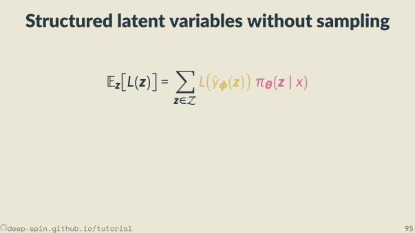
Structured latent variables without sampling
EzL(z)=∑z∈Z
Lyφ(z)πθ(z | x)
How to de ne πθ? ∑h∈H
∂EL(z)
∂θidea 1 πθ(z) ∝ exp
fθ(z)
so maxidea 2 πθ(z) = 1 if z =MAP(fθ(·)) else 0 argmaxidea 3 SparseMAP
e.g., a TreeLSTM de ned by zsum overall possible trees
parsing model,using some scorer fθ(z; x)
Exponen ally large sum!
All methods we’ve seen require sampling; hard in general.STE / SPIGOT relax y in backward.
deep-spin.github.io/tutorial 95
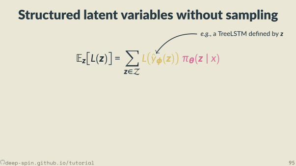
Structured latent variables without sampling
EzL(z)=∑z∈Z
Lyφ(z)πθ(z | x)
How to de ne πθ? ∑h∈H
∂EL(z)
∂θidea 1 πθ(z) ∝ exp
fθ(z)
so maxidea 2 πθ(z) = 1 if z =MAP(fθ(·)) else 0 argmaxidea 3 SparseMAP
e.g., a TreeLSTM de ned by z
sum overall possible trees
parsing model,using some scorer fθ(z; x)
Exponen ally large sum!
All methods we’ve seen require sampling; hard in general.STE / SPIGOT relax y in backward.
deep-spin.github.io/tutorial 95
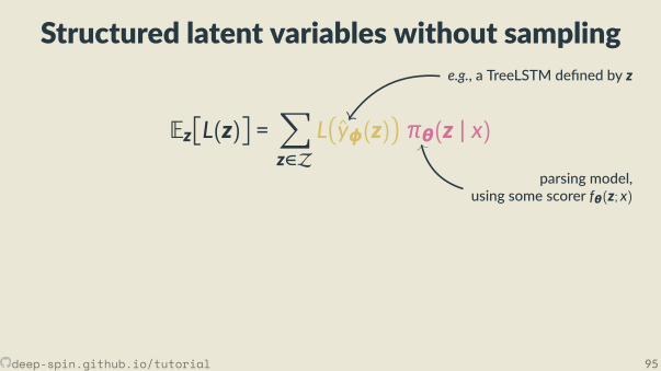
Structured latent variables without sampling
EzL(z)=∑z∈Z
Lyφ(z)πθ(z | x)
How to de ne πθ? ∑h∈H
∂EL(z)
∂θidea 1 πθ(z) ∝ exp
fθ(z)
so maxidea 2 πθ(z) = 1 if z =MAP(fθ(·)) else 0 argmaxidea 3 SparseMAP
e.g., a TreeLSTM de ned by z
sum overall possible trees
parsing model,using some scorer fθ(z; x)
Exponen ally large sum!
All methods we’ve seen require sampling; hard in general.STE / SPIGOT relax y in backward.
deep-spin.github.io/tutorial 95
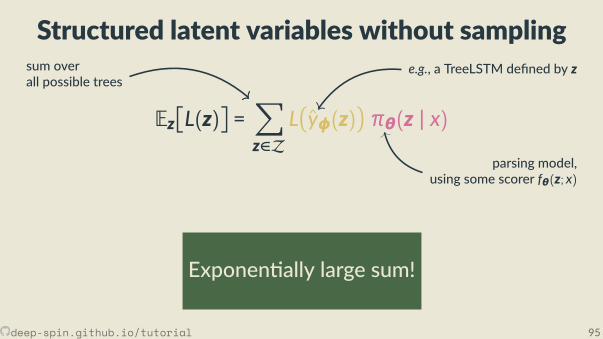
Structured latent variables without sampling
EzL(z)=∑z∈Z
Lyφ(z)πθ(z | x)
How to de ne πθ? ∑h∈H
∂EL(z)
∂θidea 1 πθ(z) ∝ exp
fθ(z)
so maxidea 2 πθ(z) = 1 if z =MAP(fθ(·)) else 0 argmaxidea 3 SparseMAP
e.g., a TreeLSTM de ned by zsum overall possible trees
parsing model,using some scorer fθ(z; x)
Exponen ally large sum!
All methods we’ve seen require sampling; hard in general.STE / SPIGOT relax y in backward.
deep-spin.github.io/tutorial 95
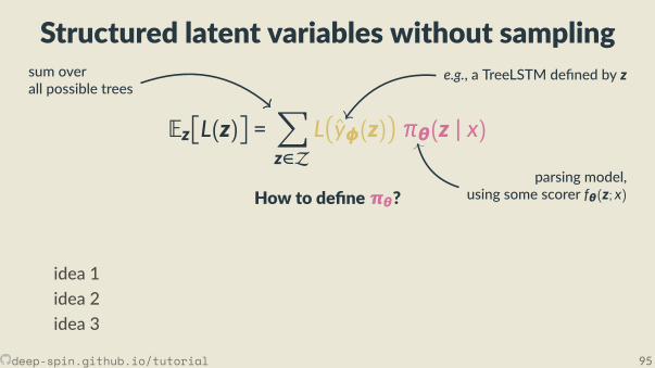
Structured latent variables without sampling
EzL(z)=∑z∈Z
Lyφ(z)πθ(z | x)
How to de ne πθ?
∑h∈H
∂EL(z)
∂θ
idea 1
πθ(z) ∝ expfθ(z)
so max
idea 2
πθ(z) = 1 if z =MAP(fθ(·)) else 0 argmax
idea 3
SparseMAP
e.g., a TreeLSTM de ned by zsum overall possible trees
parsing model,using some scorer fθ(z; x)
Exponen ally large sum!
All methods we’ve seen require sampling; hard in general.STE / SPIGOT relax y in backward.
deep-spin.github.io/tutorial 95
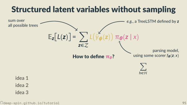
Structured latent variables without sampling
EzL(z)=∑z∈Z
Lyφ(z)πθ(z | x)
How to de ne πθ? ∑h∈H
∂EL(z)
∂θ
idea 1
πθ(z) ∝ expfθ(z)
so max
idea 2
πθ(z) = 1 if z =MAP(fθ(·)) else 0 argmax
idea 3
SparseMAP
e.g., a TreeLSTM de ned by zsum overall possible trees
parsing model,using some scorer fθ(z; x)
Exponen ally large sum!
All methods we’ve seen require sampling; hard in general.STE / SPIGOT relax y in backward.
deep-spin.github.io/tutorial 95
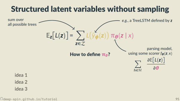
Structured latent variables without sampling
EzL(z)=∑z∈Z
Lyφ(z)πθ(z | x)
How to de ne πθ? ∑h∈H
∂EL(z)
∂θidea 1
πθ(z) ∝ expfθ(z)
so max
idea 2
πθ(z) = 1 if z =MAP(fθ(·)) else 0 argmax
idea 3
SparseMAP
e.g., a TreeLSTM de ned by zsum overall possible trees
parsing model,using some scorer fθ(z; x)
Exponen ally large sum!
All methods we’ve seen require sampling; hard in general.STE / SPIGOT relax y in backward.
deep-spin.github.io/tutorial 95
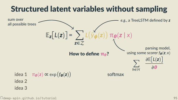
Structured latent variables without sampling
EzL(z)=∑z∈Z
Lyφ(z)πθ(z | x)
How to de ne πθ? ∑h∈H
∂EL(z)
∂θidea 1 πθ(z) ∝ exp
fθ(z)
so maxidea 2
πθ(z) = 1 if z =MAP(fθ(·)) else 0 argmax
idea 3
SparseMAP
e.g., a TreeLSTM de ned by zsum overall possible trees
parsing model,using some scorer fθ(z; x)
Exponen ally large sum!
All methods we’ve seen require sampling; hard in general.STE / SPIGOT relax y in backward.
deep-spin.github.io/tutorial 95
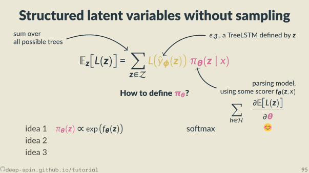
Structured latent variables without sampling
EzL(z)=∑z∈Z
Lyφ(z)πθ(z | x)
How to de ne πθ? ∑h∈H
∂EL(z)
∂θidea 1 πθ(z) ∝ exp
fθ(z)
so maxidea 2
πθ(z) = 1 if z =MAP(fθ(·)) else 0 argmax
idea 3
SparseMAP
e.g., a TreeLSTM de ned by zsum overall possible trees
parsing model,using some scorer fθ(z; x)
Exponen ally large sum!
All methods we’ve seen require sampling; hard in general.STE / SPIGOT relax y in backward.
deep-spin.github.io/tutorial 95
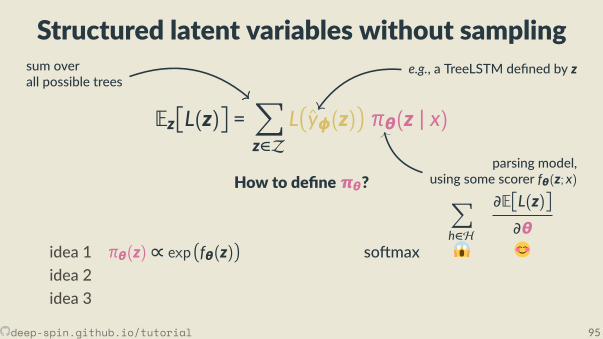
Structured latent variables without sampling
EzL(z)=∑z∈Z
Lyφ(z)πθ(z | x)
How to de ne πθ? ∑h∈H
∂EL(z)
∂θidea 1 πθ(z) ∝ exp
fθ(z)
so maxidea 2
πθ(z) = 1 if z =MAP(fθ(·)) else 0 argmax
idea 3
SparseMAP
e.g., a TreeLSTM de ned by zsum overall possible trees
parsing model,using some scorer fθ(z; x)
Exponen ally large sum!
All methods we’ve seen require sampling; hard in general.STE / SPIGOT relax y in backward.
deep-spin.github.io/tutorial 95
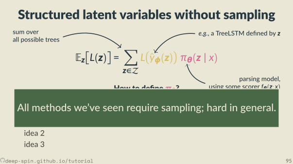
Structured latent variables without sampling
EzL(z)=∑z∈Z
Lyφ(z)πθ(z | x)
How to de ne πθ? ∑h∈H
∂EL(z)
∂θidea 1 πθ(z) ∝ exp
fθ(z)
so maxidea 2
πθ(z) = 1 if z =MAP(fθ(·)) else 0 argmax
idea 3
SparseMAP
e.g., a TreeLSTM de ned by zsum overall possible trees
parsing model,using some scorer fθ(z; x)
Exponen ally large sum!
All methods we’ve seen require sampling; hard in general.
STE / SPIGOT relax y in backward.
deep-spin.github.io/tutorial 95
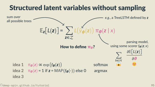
Structured latent variables without sampling
EzL(z)=∑z∈Z
Lyφ(z)πθ(z | x)
How to de ne πθ? ∑h∈H
∂EL(z)
∂θidea 1 πθ(z) ∝ exp
fθ(z)
so maxidea 2 πθ(z) = 1 if z =MAP(fθ(·)) else 0 argmaxidea 3
SparseMAP
e.g., a TreeLSTM de ned by zsum overall possible trees
parsing model,using some scorer fθ(z; x)
Exponen ally large sum!
All methods we’ve seen require sampling; hard in general.STE / SPIGOT relax y in backward.
deep-spin.github.io/tutorial 95
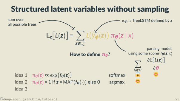
Structured latent variables without sampling
EzL(z)=∑z∈Z
Lyφ(z)πθ(z | x)
How to de ne πθ? ∑h∈H
∂EL(z)
∂θidea 1 πθ(z) ∝ exp
fθ(z)
so maxidea 2 πθ(z) = 1 if z =MAP(fθ(·)) else 0 argmaxidea 3
SparseMAP
e.g., a TreeLSTM de ned by zsum overall possible trees
parsing model,using some scorer fθ(z; x)
Exponen ally large sum!
All methods we’ve seen require sampling; hard in general.STE / SPIGOT relax y in backward.
deep-spin.github.io/tutorial 95
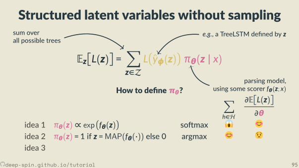
Structured latent variables without sampling
EzL(z)=∑z∈Z
Lyφ(z)πθ(z | x)
How to de ne πθ? ∑h∈H
∂EL(z)
∂θidea 1 πθ(z) ∝ exp
fθ(z)
so maxidea 2 πθ(z) = 1 if z =MAP(fθ(·)) else 0 argmaxidea 3
SparseMAP
e.g., a TreeLSTM de ned by zsum overall possible trees
parsing model,using some scorer fθ(z; x)
Exponen ally large sum!
All methods we’ve seen require sampling; hard in general.STE / SPIGOT relax y in backward.
deep-spin.github.io/tutorial 95
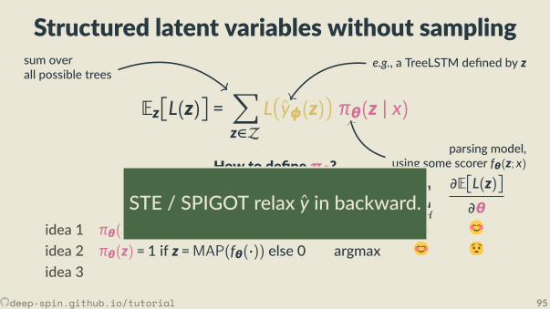
Structured latent variables without sampling
EzL(z)=∑z∈Z
Lyφ(z)πθ(z | x)
How to de ne πθ? ∑h∈H
∂EL(z)
∂θidea 1 πθ(z) ∝ exp
fθ(z)
so maxidea 2 πθ(z) = 1 if z =MAP(fθ(·)) else 0 argmaxidea 3
SparseMAP
e.g., a TreeLSTM de ned by zsum overall possible trees
parsing model,using some scorer fθ(z; x)
Exponen ally large sum!
All methods we’ve seen require sampling; hard in general.
STE / SPIGOT relax y in backward.
deep-spin.github.io/tutorial 95
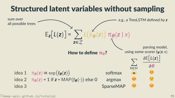
Structured latent variables without sampling
EzL(z)=∑z∈Z
Lyφ(z)πθ(z | x)
How to de ne πθ? ∑h∈H
∂EL(z)
∂θidea 1 πθ(z) ∝ exp
fθ(z)
so maxidea 2 πθ(z) = 1 if z =MAP(fθ(·)) else 0 argmaxidea 3 SparseMAP
e.g., a TreeLSTM de ned by zsum overall possible trees
parsing model,using some scorer fθ(z; x)
Exponen ally large sum!
All methods we’ve seen require sampling; hard in general.STE / SPIGOT relax y in backward.
deep-spin.github.io/tutorial 95
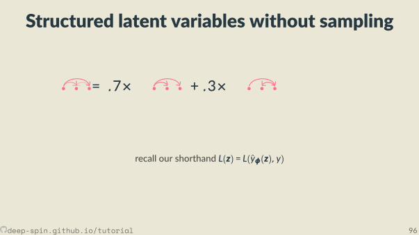
Structured latent variables without sampling
• • •= .7× • • • + .3× • • •
+0× • • • + ...E[L(z)]= .7× L( • • •)+ .3× L( • • • )
recall our shorthand L(z) = L(yφ(z), y)
deep-spin.github.io/tutorial 96
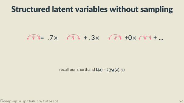
Structured latent variables without sampling
• • •= .7× • • • + .3× • • • +0× • • • + ...
E[L(z)]= .7× L( • • •)+ .3× L( • • • )
recall our shorthand L(z) = L(yφ(z), y)
deep-spin.github.io/tutorial 96
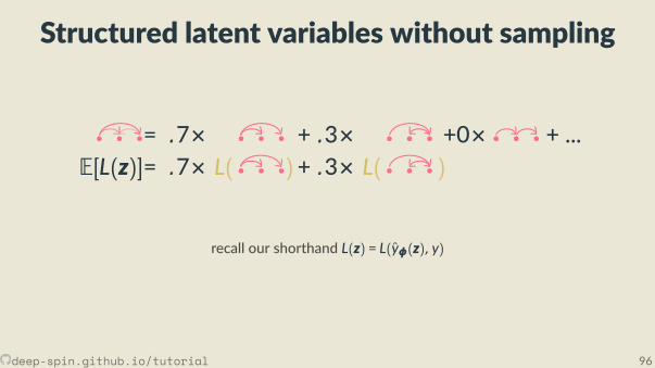
Structured latent variables without sampling
• • •= .7× • • • + .3× • • • +0× • • • + ...E[L(z)]= .7× L( • • •)+ .3× L( • • • )
recall our shorthand L(z) = L(yφ(z), y)
deep-spin.github.io/tutorial 96
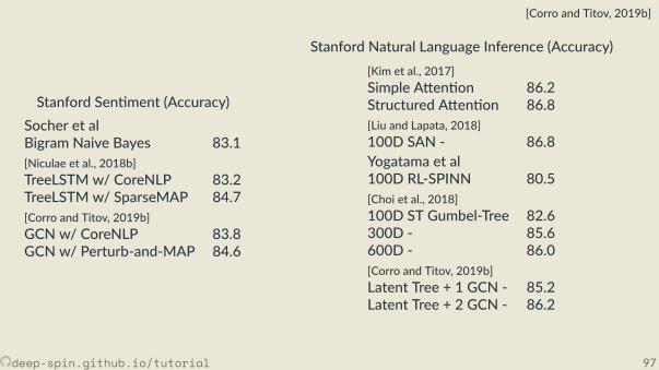
[Corro and Titov, 2019b]
Stanford Sen ment (Accuracy)Socher et alBigram Naive Bayes 83.1[Niculae et al., 2018b]TreeLSTM w/ CoreNLP 83.2TreeLSTM w/ SparseMAP 84.7[Corro and Titov, 2019b]GCN w/ CoreNLP 83.8GCN w/ Perturb-and-MAP 84.6
Stanford Natural Language Inference (Accuracy)[Kim et al., 2017]Simple A en on 86.2Structured A en on 86.8[Liu and Lapata, 2018]100D SAN - 86.8Yogatama et al100D RL-SPINN 80.5[Choi et al., 2018]100D ST Gumbel-Tree 82.6300D - 85.6600D - 86.0[Corro and Titov, 2019b]Latent Tree + 1 GCN - 85.2Latent Tree + 2 GCN - 86.2
deep-spin.github.io/tutorial 97
V. Conclusions
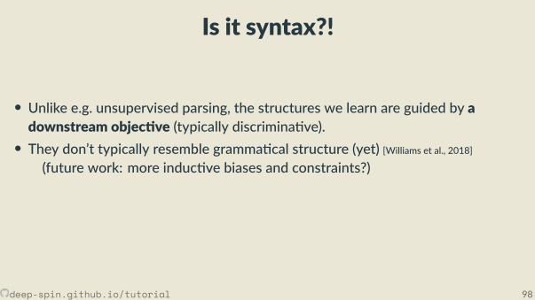
Is it syntax?!
• Unlike e.g. unsupervised parsing, the structures we learn are guided by adownstream objec ve (typically discrimina ve).• They don’t typically resemble gramma cal structure (yet) [Williams et al., 2018]
(future work: more induc ve biases and constraints?)
• Common to compare latent structures with parser outputs.But is this always a meaningful comparison?
deep-spin.github.io/tutorial 98
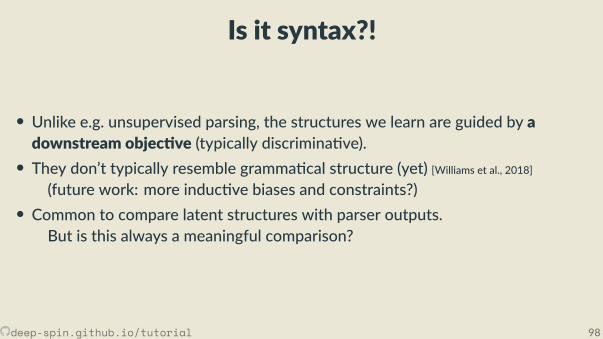
Is it syntax?!
• Unlike e.g. unsupervised parsing, the structures we learn are guided by adownstream objec ve (typically discrimina ve).• They don’t typically resemble gramma cal structure (yet) [Williams et al., 2018]
(future work: more induc ve biases and constraints?)• Common to compare latent structures with parser outputs.
But is this always a meaningful comparison?
deep-spin.github.io/tutorial 98
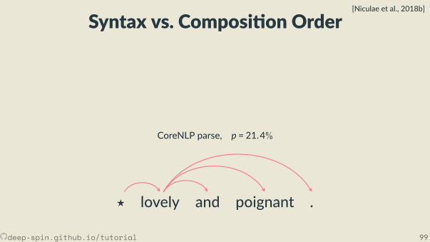
Syntax vs. Composi on Order[Niculae et al., 2018b]
p = 22.6%
⋆ lovely and poignant .
CoreNLP parse, p = 21.4%
⋆ lovely and poignant .
· · ·
deep-spin.github.io/tutorial 99
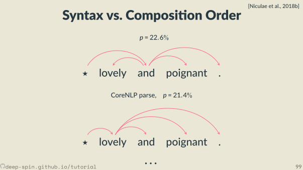
Syntax vs. Composi on Order[Niculae et al., 2018b]
p = 22.6%
⋆ lovely and poignant .
CoreNLP parse, p = 21.4%
⋆ lovely and poignant .
· · ·deep-spin.github.io/tutorial 99
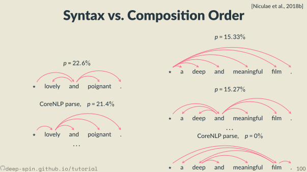
Syntax vs. Composi on Order[Niculae et al., 2018b]
p = 22.6%
⋆ lovely and poignant .
CoreNLP parse, p = 21.4%
⋆ lovely and poignant .
· · ·
p = 15.33%
⋆ a deep and meaningful lm .1.0 1.0
1.01.0
1.0 1.0
p = 15.27%
⋆ a deep and meaningful lm .
1.01.0
1.01.0
1.01.0
· · ·CoreNLP parse, p = 0%
⋆ a deep and meaningful lm .
1.0 1.0
1.01.0
1.0
1.0
deep-spin.github.io/tutorial 100
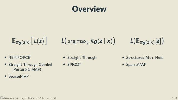
Overview
Eπθ(z|x)L(z)
• REINFORCE• Straight-Through Gumbel
(Perturb & MAP)• SparseMAP
Largmaxz πθ(z | x)
• Straight-Through• SPIGOT
LEπθ(z|x)[z]
• Structured A n. Nets• SparseMAP
And more, a er the break!
deep-spin.github.io/tutorial 101
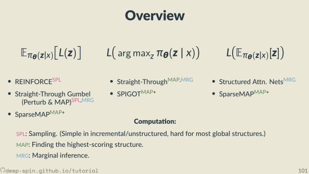
Overview
Eπθ(z|x)L(z)
• REINFORCESPL• Straight-Through Gumbel
(Perturb & MAP)SPL,MRG
• SparseMAPMAP+
Largmaxz πθ(z | x)
• Straight-ThroughMAP,MRG• SPIGOTMAP+
LEπθ(z|x)[z]
• Structured A n. NetsMRG
• SparseMAPMAP+
Computa on:
SPL: Sampling. (Simple in incremental/unstructured, hard for most global structures.)MAP: Finding the highest-scoring structure.MRG: Marginal inference.
And more, a er the break!
deep-spin.github.io/tutorial 101
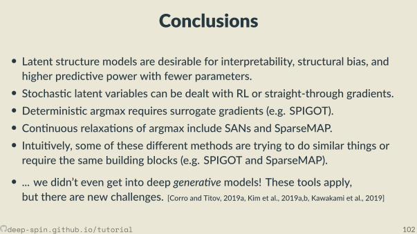
Conclusions
• Latent structure models are desirable for interpretability, structural bias, andhigher predic ve power with fewer parameters.• Stochas c latent variables can be dealt with RL or straight-through gradients.• Determinis c argmax requires surrogate gradients (e.g. SPIGOT).• Con nuous relaxa ons of argmax include SANs and SparseMAP.• Intui vely, some of these di erent methods are trying to do similar things orrequire the same building blocks (e.g. SPIGOT and SparseMAP).
• ... we didn’t even get into deep genera ve models! These tools apply,but there are new challenges. [Corro and Titov, 2019a, Kim et al., 2019a,b, Kawakami et al., 2019]
deep-spin.github.io/tutorial 102
References IRyan Adams. The gumbel-max trick for discrete distribu ons, 2013. URL
https://lips.cs.princeton.edu/the-gumbel-max-trick-for-discrete-distributions/. Blog post.James K Baker. Trainable grammars for speech recogni on. The Journal of the Acous cal Society of America, 65(S1):S132–S132,1979.
Yoshua Bengio, Nicholas Léonard, and Aaron Courville. Es ma ng or propaga ng gradients through stochas c neurons forcondi onal computa on. arXiv preprint arXiv:1308.3432, 2013.
Mathieu Blondel, André FT Mar ns, and Vlad Niculae. Learning classi ers with Fenchel-Young losses: Generalized entropies,margins, and algorithms. In Proc. of AISTATS, 2019.
Samuel R. Bowman, Jon Gauthier, Abhinav Rastogi, Raghav Gupta, Christopher D. Manning, and Christopher Po s. A fast uni edmodel for parsing and sentence understanding. In Proc. of ACL, 2016. doi: 10.18653/v1/P16-1139.
Stephen Boyd and Lieven Vandenberghe. Convex op miza on. Cambridge University Press, 2004.Peter F Brown, Vincent J Della Pietra, Stephen A Della Pietra, and Robert L Mercer. The mathema cs of sta s cal machinetransla on: Parameter es ma on. Computa onal Linguis cs, 19(2):263–311, 1993.
Qian Chen, Xiaodan Zhu, Zhen-Hua Ling, Si Wei, Hui Jiang, and Diana Inkpen. Enhanced LSTM for natural language inference. InProc. of ACL, 2017.
Jihun Choi, Kang Min Yoo, and Sang-goo Lee. Learning to compose task-speci c tree structures. In Proc. of AAAI, 2018.
deep-spin.github.io/tutorial 103
References IIYoeng-Jin Chu and Tseng-Hong Liu. On the shortest arborescence of a directed graph. Science Sinica, 14:1396–1400, 1965.William John Cocke and Jacob T Schwartz. Programming languages and their compilers. Courant Ins tute of Mathema calSciences., 1970.
Shay B Cohen, Karl Stratos, Michael Collins, Dean P Foster, and Lyle Ungar. Spectral learning of latent-variable PCFGs. In Proc. ofACL, 2012.
Caio Corro and Ivan Titov. Di eren able Perturb-and-Parse: Semi-Supervised Parsing with a Structured Varia onal Autoencoder.In Proc. of ICLR, 2019a.
Caio Corro and Ivan Titov. Learning latent trees with stochas c perturba ons and di eren able dynamic programming. In Proc.of ACL, 2019b.
Marco Cuturi and Mathieu Blondel. So -DTW: a di eren able loss func on for me-series. In Proc. of ICML, 2017.Jack Edmonds. Op mum branchings. J. Res. Nat. Bur. Stand., 71B:233–240, 1967.Marguerite Frank and Philip Wolfe. An algorithm for quadra c programming. Nav. Res. Log., 3(1-2):95–110, 1956.Serhii Havrylov, Germán Kruszewski, and Armand Joulin. Coopera ve Learning of Disjoint Syntax and Seman cs. In Proc.
NAACL-HLT, 2019.Geo rey Hinton. Neural networks for machine learning. In Coursera video lectures, 2012.Eric Jang, Shixiang Gu, and Ben Poole. Categorical reparameteriza on with Gumbel-so max. In Proc. of ICLR, 2017.
deep-spin.github.io/tutorial 104
References IIIRoy Jonker and Anton Volgenant. A shortest augmen ng path algorithm for dense and sparse linear assignment problems.
Compu ng, 38(4):325–340, 1987.Tadao Kasami. An e cient recogni on and syntax-analysis algorithm for context-free languages. Coordinated Science Laboratory
Report no. R-257, 1966.Kazuya Kawakami, Chris Dyer, and Phil Blunsom. Learning to discover, ground and use words with segmental neural languagemodels. In Proc. of ACL, 2019.
Yoon Kim, Carl Denton, Loung Hoang, and Alexander M Rush. Structured a en on networks. In Proc. of ICLR, 2017.Yoon Kim, Chris Dyer, and Alexander Rush. Compound probabilis c context-free grammars for grammar induc on. In Proc. of
ACL, 2019a.Yoon Kim, Alexander Rush, Lei Yu, Adhiguna Kuncoro, Chris Dyer, and Gábor Melis. Unsupervised recurrent neural networkgrammars. In Proc. of NAACL-HLT, 2019b.
Diederik P Kingma and Max Welling. Auto-encoding Varia onal Bayes. 2014.Gustav Kirchho . Ueber die au ösung der gleichungen, auf welche man bei der untersuchung der linearen vertheilunggalvanischer ströme geführt wird. Annalen der Physik, 148(12):497–508, 1847.
Harold W Kuhn. The Hungarian method for the assignment problem. Nav. Res. Log., 2(1-2):83–97, 1955.Simon Lacoste-Julien and Mar n Jaggi. On the global linear convergence of Frank-Wolfe op miza on variants. In Proc. of
NeurIPS, 2015.
deep-spin.github.io/tutorial 105
References IVZhifei Li and Jason Eisner. First-and second-order expecta on semirings with applica ons to minimum-risk training ontransla on forests. In Proc. of EMNLP, 2009.
Yang Liu and Mirella Lapata. Learning structured text representa ons. TACL, 6:63–75, 2018.Chris J Maddison, Andriy Mnih, and Yee Whye Teh. The concrete distribu on: A con nuous relaxa on of discrete randomvariables. In Proc. of ICLR, 2016.
Jean Maillard and Stephen Clark. Latent tree learning with di eren able parsers: Shi -Reduce parsing and chart parsing. arXivpreprint arXiv:1806.00840, 2018.
Chaitanya Malaviya, Pedro Ferreira, and André FT Mar ns. Sparse and constrained a en on for neural machine transla on. InProc. of ACL, 2018.
André FT Mar ns and Ramón Fernandez Astudillo. From so max to sparsemax: A sparse model of a en on and mul -labelclassi ca on. In Proc. of ICML, 2016.
André FT Mar ns and Julia Kreutzer. Learning what’s easy: Fully di eren able neural easy- rst taggers. In Proc. of EMNLP, 2017.André FT Mar ns and Vlad Niculae. Notes on latent structure models and SPIGOT. preprint arXiv:1907.10348, 2019.André FT Mar ns, Mário AT Figueiredo, Pedro MQ Aguiar, Noah A Smith, and Eric P Xing. AD3: Alterna ng direc ons dualdecomposi on for MAP inference in graphical models. JMLR, 16(1):495–545, 2015.
Arthur Mensch and Mathieu Blondel. Di eren able dynamic programming for structured predic on and a en on. In Proc. ofICML, 2018.
deep-spin.github.io/tutorial 106
References VNikita Nangia and Samuel Bowman. ListOps: A diagnos c dataset for latent tree learning. In Proc. of NAACL SRW, 2018.Vlad Niculae and Mathieu Blondel. A regularized framework for sparse and structured neural a en on. In Proc. of NeurIPS, 2017.Vlad Niculae, André FT Mar ns, Mathieu Blondel, and Claire Cardie. SparseMAP: Di eren able sparse structured inference. In
Proc. of ICML, 2018a.Vlad Niculae, André FT Mar ns, and Claire Cardie. Towards dynamic computa on graphs via sparse latent structure. In Proc. of
EMNLP, 2018b.Jorge Nocedal and Stephen Wright. Numerical Op miza on. Springer New York, 1999.George Papandreou and Alan L Yuille. Perturb-and-MAP random elds: Using discrete op miza on to learn and sample fromenergy models. In Proc. of ICCV, 2011.
Hao Peng, Sam Thomson, and Noah A Smith. Backpropaga ng through structured argmax using a SPIGOT. In Proc. of ACL, 2018.Ben Peters, Vlad Niculae, and André FT Mar ns. Sparse sequence-to-sequence models. In Proc. of ACL, 2019.Slav Petrov and Dan Klein. Discrimina ve log-linear grammars with latent variables. In Advances in neural informa on processing
systems, pages 1153–1160, 2008.Ariadna Qua oni, Sybor Wang, Louis-Philippe Morency, Michael Collins, and Trevor Darrell. Hidden condi onal random elds.
IEEE Transac ons on Pa ern Analysis & Machine Intelligence, 29(10):1848–1852, 2007.
deep-spin.github.io/tutorial 107
References VILawrence R. Rabiner. A tutorial on Hidden Markov Models and selected applica ons in speech recogni on. P. IEEE, 77(2):257–286, 1989.
Hiroaki Sakoe and Seibi Chiba. Dynamic programming algorithm op miza on for spoken word recogni on. IEEE Trans. onAcous cs, Speech, and Sig. Proc., 26:43–49, 1978.
Veselin Stoyanov, Alexander Ropson, and Jason Eisner. Empirical risk minimiza on of graphical model parameters givenapproximate inference, decoding, and model structure. In Proc. of AISTATS, 2011.
Ben Taskar. Learning structured predic on models: A large margin approach. PhD thesis, Stanford University, 2004.Constan no Tsallis. Possible generaliza on of Boltzmann-Gibbs sta s cs. Journal of Sta s cal Physics, 52:479–487, 1988.Leslie G Valiant. The complexity of compu ng the permanent. Theor. Comput. Sci., 8(2):189–201, 1979.Tim Vieira. Gumbel-max trick, 2014. URL
https://timvieira.github.io/blog/post/2014/07/31/gumbel-max-trick/. Blog post.Marina Vinyes and Guillaume Obozinski. Fast column genera on for atomic norm regulariza on. In Proc. of AISTATS, 2017.Mar n J Wainwright and Michael I Jordan. Graphical models, exponen al families, and varia onal inference., volume 1. NowPublishers, Inc., 2008.
Adina Williams, Andrew Drozdov, and Samuel R Bowman. Do latent tree learning models iden fy meaningful structure insentences? TACL, 2018.
deep-spin.github.io/tutorial 108
References VIIRonald J. Williams. Simple sta s cal gradient-following algorithms for connec onist reinforcement learning. Mach. Learn., 8,1992.
Philip Wolfe. Finding the nearest point in a polytope. Mathema cal Programming, 11(1):128–149, 1976.Dani Yogatama, Phil Blunsom, Chris Dyer, Edward Grefenste e, and Wang Ling. Learning to compose words into sentences withreinforcement learning. In Proc. of ICLR, 2017.
Daniel H Younger. Recogni on and parsing of context-free languages in me n3. Informa on and Control, 10(2):189–208, 1967.
deep-spin.github.io/tutorial 109