Embed Size (px)
Citation preview
8/13/2019 Lect9_sys Char & Routh
http://slidepdf.com/reader/full/lect9sys-char-routh 1/15
CONTROL SYSTEM I
System Characteristics
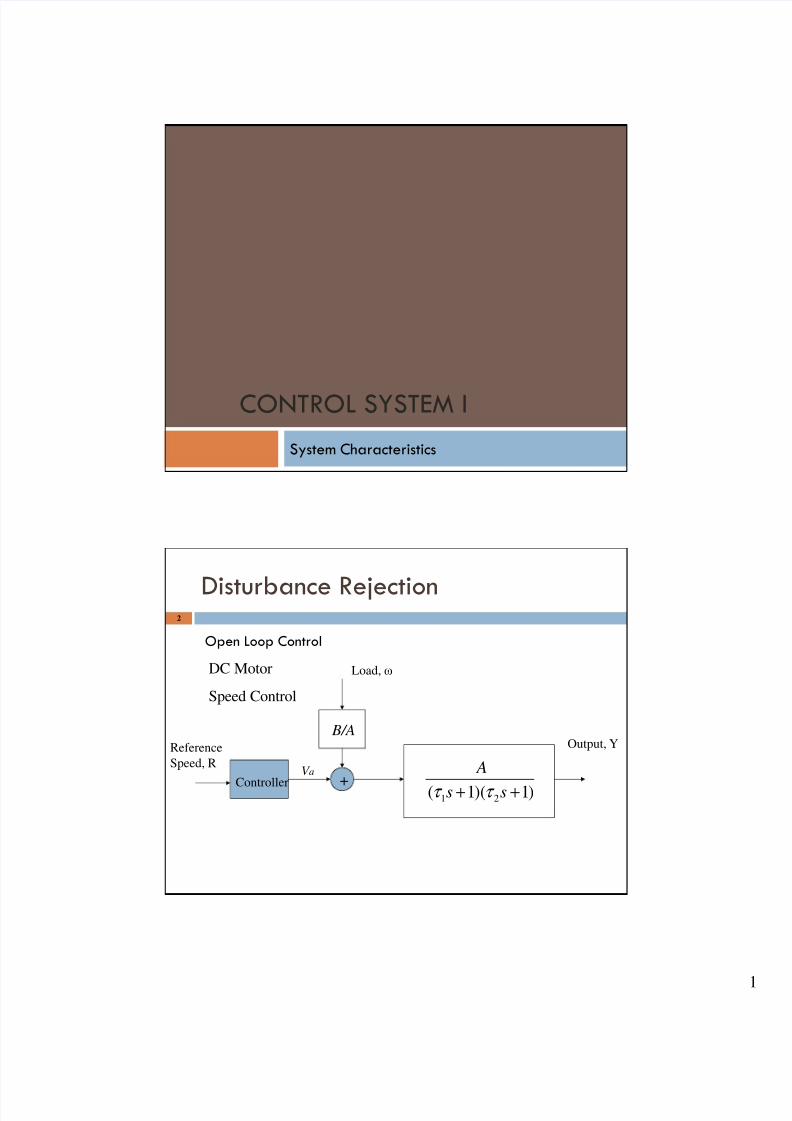
Disturbance Rejection
Open Loop Control
+
B/A
Controller
Reference
Speed, R
)1)(1( 21 ++ ss
A
τ τ
V a
Output, Y
Load, ωDC Motor
Speed Control
2
8/13/2019 Lect9_sys Char & Routh
http://slidepdf.com/reader/full/lect9sys-char-routh 2/15
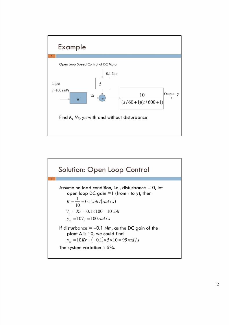
Example
Open Loop Speed Control of DC Motor
Find K, V a, yss with and without disturbance
+
5
K
Input
r=100 rad/s
)1600 / )(160 / (
10
++ ss
VaOutput, y
-0.1 Nm
3
Solution: Open Loop Control
Assume no load condition, i.e., disturbance = 0, letopen loop DC gain =1 (from r to y), then
If disturbance = –0.1 Nm, as the DC gain of theplant A is 10, we could find
The system variation is 5%.
4
( )
( ) srad Kr y
srad V y
volt Kr V
srad volt K
ss
ass
a
/ 951051.010
/ 10010
101001.0
/ / 1.010
1
=××−+=
==
=×==
==
8/13/2019 Lect9_sys Char & Routh
http://slidepdf.com/reader/full/lect9sys-char-routh 3/15
Example5
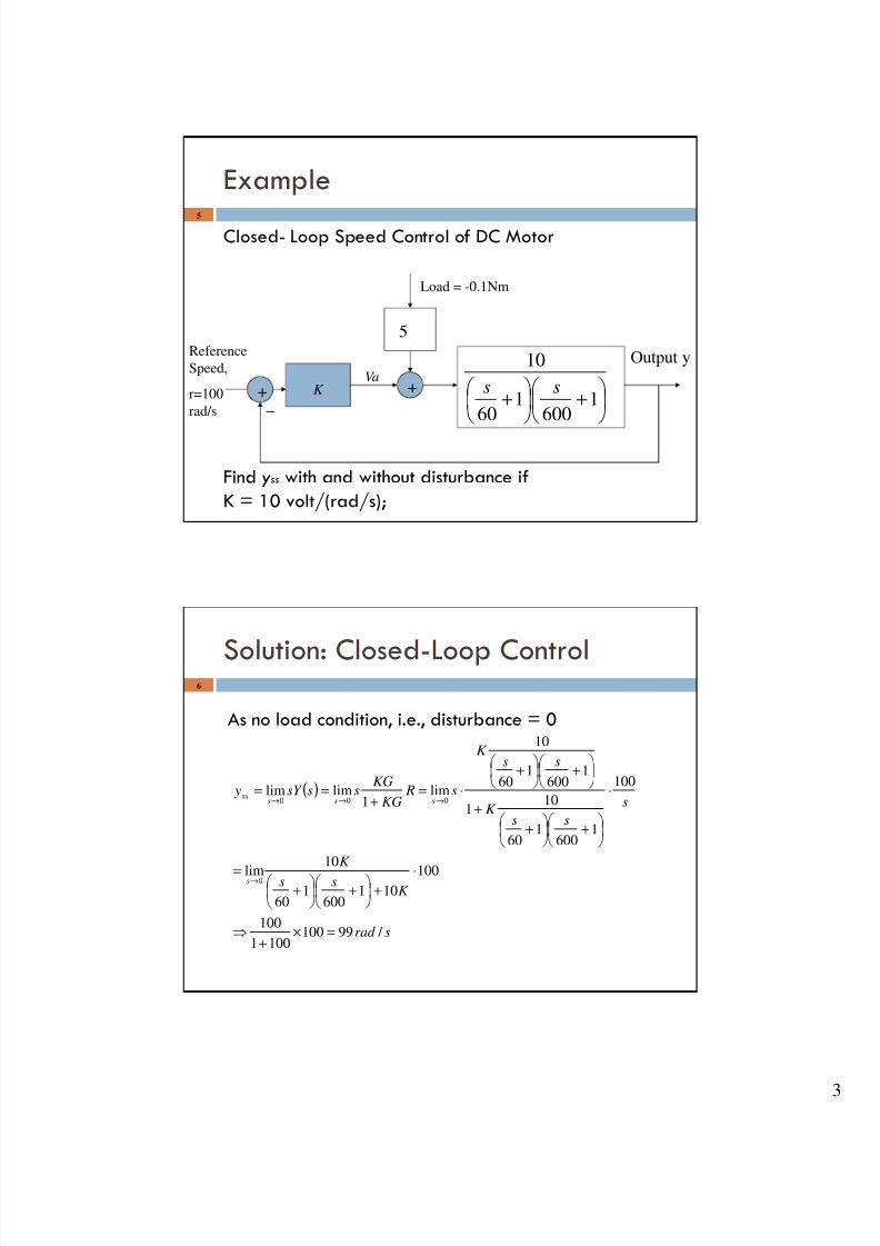
Closed- Loop Speed Control of DC Motor
Find yss with and without disturbance if
K = 10 volt/(rad/s);
+
5
K
Reference
Speed,
r=100
rad/s
+
+ 1
6001
60
10
ssVa
Load = -0.1Nm
+_
Output y
Solution: Closed-Loop Control
As no load condition, i.e., disturbance = 0
6
( )
srad
K ss
K
s
ssK
ssK
s RKG
KGsssY y
s
sssss
/ 991001001
100
100101
6001
60
10
lim
100
1600
160
101
1600
160
10
lim1
limlim
0
000
=×
+
⇒
⋅
+
+
+
=
⋅
+
+
+
+
+
⋅=
+
==
→
→→→
8/13/2019 Lect9_sys Char & Routh
http://slidepdf.com/reader/full/lect9sys-char-routh 4/15
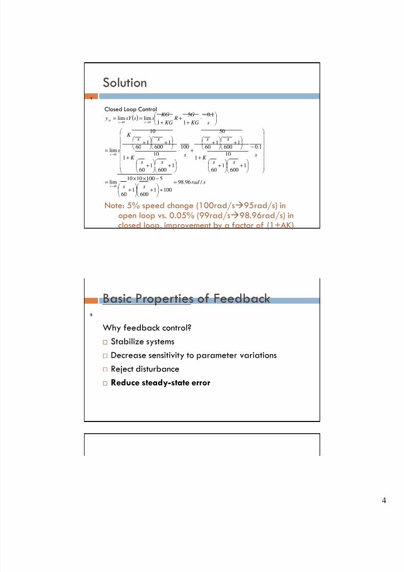
Solution
Closed Loop Control
Note: 5% speed change (100rad/s95rad/s) inopen loop vs. 0.05% (99rad/s98.96rad/s) inclosed loop, improvement by a factor of (1+AK)
7
( )
srad ss
s
ssK
ss
s
ssK
ssK
s
sKG
G R
KG
KGsssY y
s
s
ssss
/ 96.98
1001600
160
51001010lim
1.0
1600
160
101
1600
160
50
100
1600
160
101
1600
160
10
lim
1.0
1
5
1limlim
0
0
00
=
+
+
+
−××=
−
+
+
+
+
+
+⋅
+
+
+
+
+
=
−⋅
+
+
+
==
→
→
→→
Basic Properties of Feedback
Why feedback control?
Stabilize systems
Decrease sensitivity to parameter variations
Reject disturbance
Reduce steady-state error
8
8/13/2019 Lect9_sys Char & Routh
http://slidepdf.com/reader/full/lect9sys-char-routh 5/15
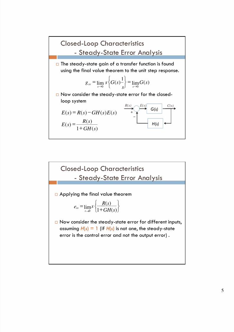
Closed-Loop Characteristics
- Steady-State Error Analysis
The steady-state gain of a transfer function is found
using the final value theorem to the unit step response.
Now consider the steady-state error for the closed-
loop system
)(lim1
)(lim00
sGs
sGsgss
ss→→
=
=
G(s)
H(s)
E(s) R(s) C(s)
+
–
)(1
)()(
sGH
s Rs E
+
=
)()()()( s E sGH s Rs E −=
Closed-Loop Characteristics
- Steady-State Error Analysis
Applying the final value theorem
Now consider the steady-state error for different inputs,
assuming H(s) = 1 (if H(s) is not one, the steady-state
error is the control error and not the output error) .
+=
→ )(1
)(lim
0 sGH
s Rse
sss
8/13/2019 Lect9_sys Char & Routh
http://slidepdf.com/reader/full/lect9sys-char-routh 6/15
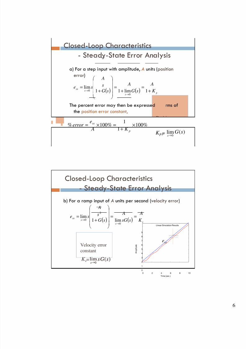
Closed-Loop Characteristics
- Steady-State Error Analysis
a) For a step input with amplitude, A units (position
error)
The percent error may then be expressed in terms of
the position error constant,
Position error
constant
ssG
→
)(lim0
pK P =
( ) ( ) ps
sss
K
A
sG
A
sG
s
A
se+
=
+
=
+
=
→
→ 1lim11lim
0
0
%1001
1%100% ×
+
=×=
p
ss
K Aeerror
Closed-Loop Characteristics
- Steady-State Error Analysis
b) For a ramp input of A units per second (velocity error)
Velocity errorconstant
ssssGGss
→→
))((limlim00
vvK ==
Time (sec.)
A m p l i t u d e
Linear Simulation Results
0 2 4 6 8 10
0
1
2
3
4
5
6
7
8
9
ess
( ) ( ) vs
sss
K
A
ssG
A
sG
s
A
se ==
+
=
→
→
0
2
0 lim1lim
8/13/2019 Lect9_sys Char & Routh
http://slidepdf.com/reader/full/lect9sys-char-routh 7/15
Closed-Loop Characteristics
- Steady-State Error Analysis
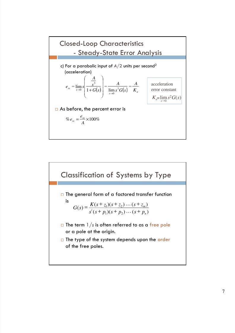
c) For a parabolic input of A/2 units per second2
(acceleration)
As before, the percent error is
acceleration
error constant
ssGs2
→
)(lim0
aK =
( ) ( )
%100%
lim1lim
2
0
3
0
×=
==
+
=
→
→
Aee
K
A
sGs
A
sG
s
A
se
ss
ss
as
sss
Classification of Systems by Type
The general form of a factored transfer function
is
The term 1/s is often referred to as a free pole
or a pole at the origin. The type of the system depends upon the order
of the free poles.
)())((
)())(()(
21
21
n
i
m
ps ps pss
zs zs zsK sG
+++
+++=
L
L
8/13/2019 Lect9_sys Char & Routh
http://slidepdf.com/reader/full/lect9sys-char-routh 8/15
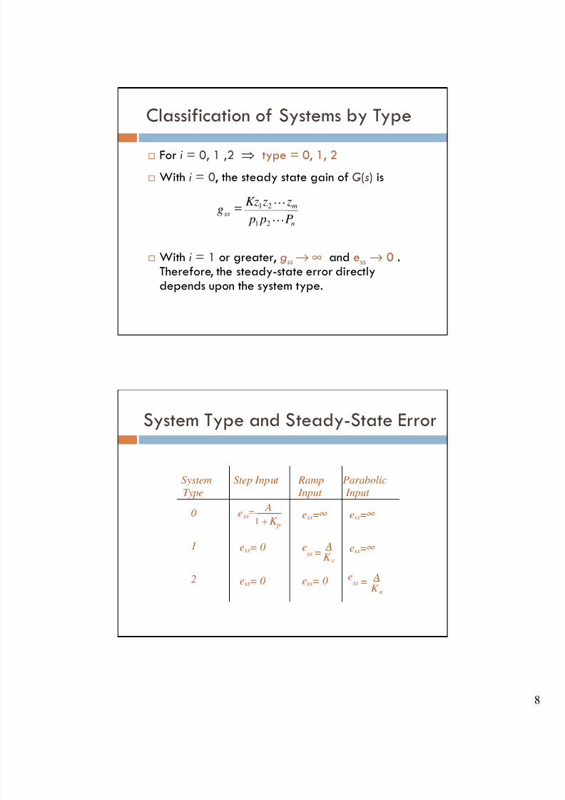
Classification of Systems by Type
For i = 0, 1 ,2 ⇒ type = 0, 1, 2
With i = 0, the steady state gain of G(s) is
With i = 1 or greater, gss → ∞ and ess → 0 .Therefore, the steady-state error directlydepends upon the system type.
n
mss
P p p
z zKzg
L
L
21
21=
System Type and Steady-State Error
System
Type
Step Input Ramp
Input
Parabolic
Input
0 ess=∞ ess=∞
1 ess= 0 ess =
A
K v
ess=∞
2 ess= 0 ess= 0
A
+ K p
=
1
ess = A
K a
ess
8/13/2019 Lect9_sys Char & Routh
http://slidepdf.com/reader/full/lect9sys-char-routh 9/15
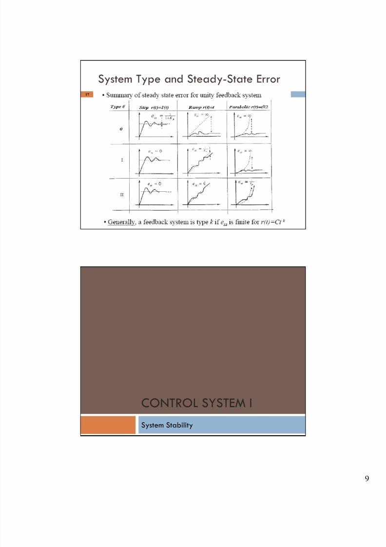
System Type and Steady-State Error
17
CONTROL SYSTEM I
System Stability
8/13/2019 Lect9_sys Char & Routh
http://slidepdf.com/reader/full/lect9sys-char-routh 10/15
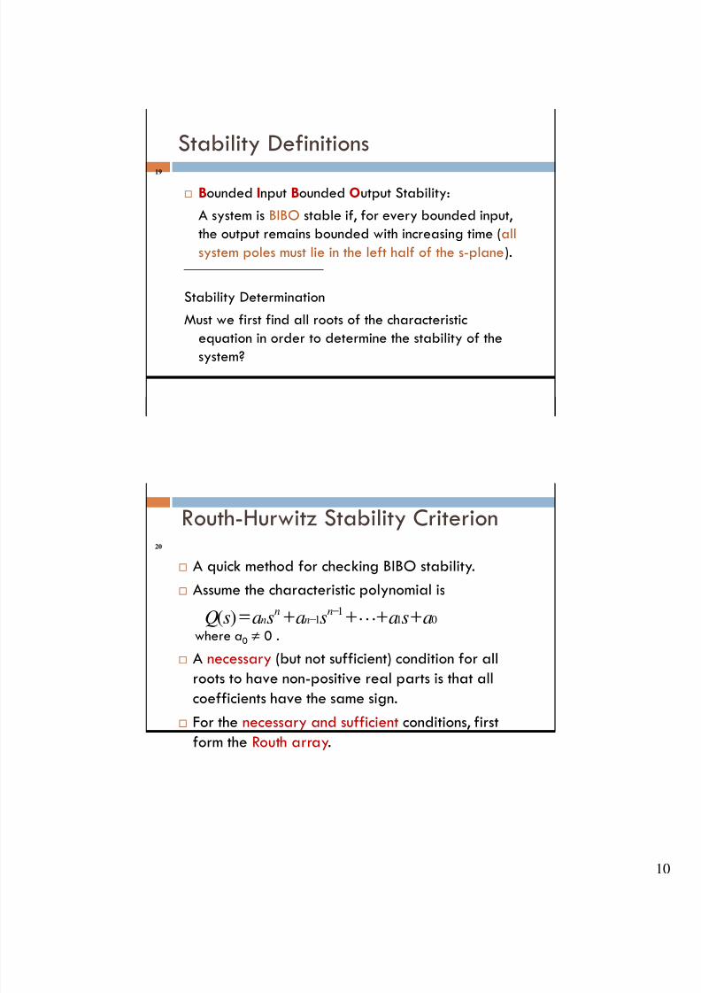
Stability Definitions
Bounded Input Bounded Output Stability:
A system is BIBO stable if, for every bounded input,
the output remains bounded with increasing time (all
system poles must lie in the left half of the s-plane).
Stability Determination
Must we first find all roots of the characteristic
equation in order to determine the stability of the
system?
19
Routh-Hurwitz Stability Criterion
A quick method for checking BIBO stability.
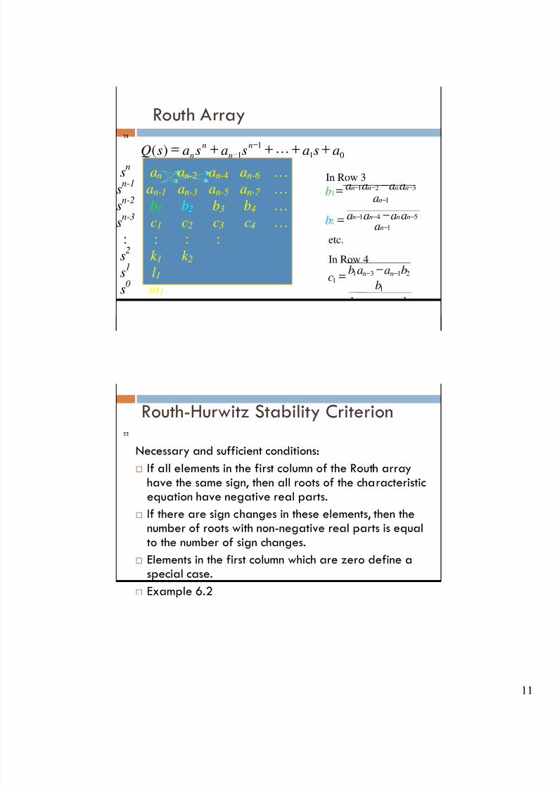
Assume the characteristic polynomial is
where a0 ≠ 0 .
A necessary (but not sufficient) condition for all
roots to have non-positive real parts is that all
coefficients have the same sign. For the necessary and sufficient conditions, first
form the Routh array.
011
1)( asasasasQ n
nn
n ++++= −
− L
20
8/13/2019 Lect9_sys Char & Routh
http://slidepdf.com/reader/full/lect9sys-char-routh 11/15
Routh Array
sn
an an-2 an-4 an-6 …
sn-1
an-1 an-3 an-5 an-7 …
sn-2
b1 b2 b3 b4 …
sn-3
c1 c2 c3 c4 …
: : : :
s2
k 1 k 2
s
1
l1s
0m1
1
5412
−
−−− −=
n
nnnn
aaaaab
1
3211
−
−−− −=
n
nnnn
aaaaa
b
In Row 3
etc.
In Row 4
01
1
1)( asasasasQ n
n
n
n ++++=
−
− L
21
1
31512
1
21311
b
baabc
b baabc
nn
nn
−−
−−
−=
−
=
The elements in all subsequent rows are
calculated in the same manner.
Routh-Hurwitz Stability Criterion
Necessary and sufficient conditions:
If all elements in the first column of the Routh arrayhave the same sign, then all roots of the characteristicequation have negative real parts.
If there are sign changes in these elements, then thenumber of roots with non-negative real parts is equalto the number of sign changes.
Elements in the first column which are zero define aspecial case.
Example 6.2
22
8/13/2019 Lect9_sys Char & Routh
http://slidepdf.com/reader/full/lect9sys-char-routh 12/15
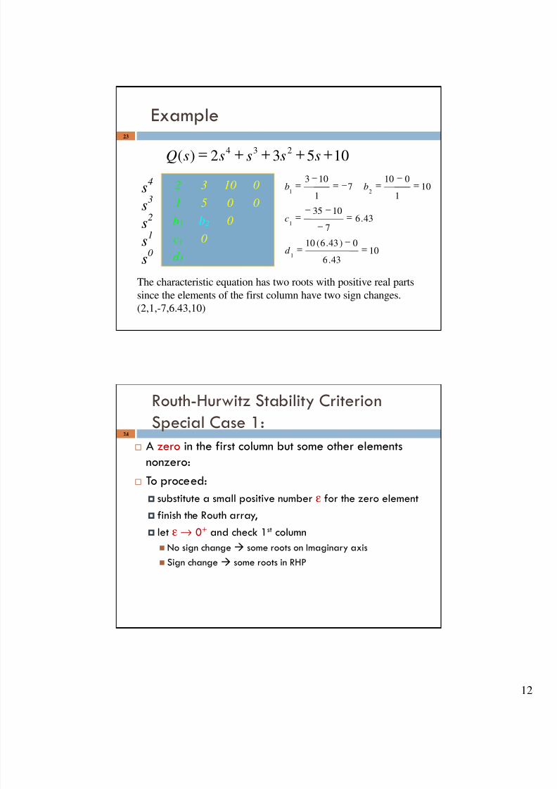
Example
10532)(234
++++= sssssQ
s4 2 3 10 0
s3 1 5 0 0
s2 b1 b2 0
s1 c1 0
s0 d 1
1043.6
0)43.6(10
43.67
1035
101
0107
1
103
1
1
21
=
−
=
=
−
−−
=
=
−
=−=
−
=
d
c
bb
The characteristic equation has two roots with positive real parts
since the elements of the first column have two sign changes.
(2,1,-7,6.43,10)
23
Routh-Hurwitz Stability Criterion
Special Case 1:
A zero in the first column but some other elements
nonzero:
To proceed:
substitute a small positive number ε for the zero element
finish the Routh array,
let ε → 0+ and check 1st column
No sign change some roots on Imaginary axis
Sign change some roots in RHP
24
8/13/2019 Lect9_sys Char & Routh
http://slidepdf.com/reader/full/lect9sys-char-routh 13/15
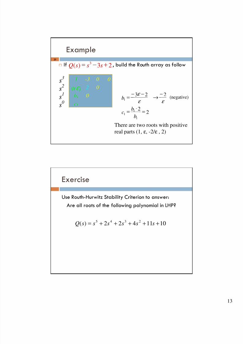
Example
If , build the Routh array as follow
s3 1 -3 0 0
s2
0(ε ) 2 0
s1 b1 0
s0 c1
23)(3
+−= sssQ
22
223
1
11
1
=⋅
=
−→
−−=
b
bc
bε ε
ε (negative)
There are two roots with positive
real parts (1, ε, -2/ ε , 2)
25
Exercise
Use Routh-Hurwitz Stability Criterion to answer:
Are all roots of the following polynomial in LHP?
1011422)( 2345
+++++= ssssssQ
8/13/2019 Lect9_sys Char & Routh
http://slidepdf.com/reader/full/lect9sys-char-routh 14/15
Routh-Hurwitz Stability Criterion
Special Case 2:
An all zero row in the Routh array which correspondsto pairs of roots with opposite signs.
To proceed:
form an auxiliary polynomial from the coefficients in therow above.
Replace the zero coefficients from the coefficients of thedifferentiated auxiliary polynomial.
Complete the array and check 1st column
No a sign change the roots of the auxiliary equation define
the roots of the system on the imaginary axis. Sign change a(s) has factors of the form
27
( )( )σ σ +− ss
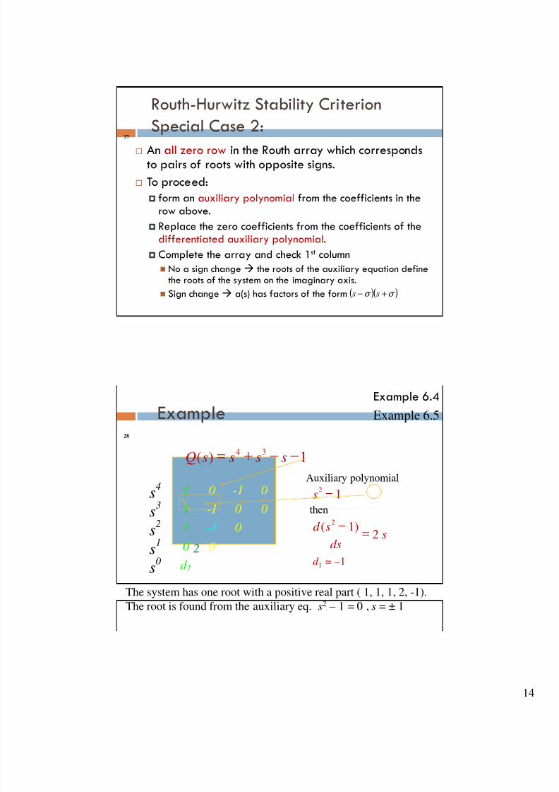
Example
1)(34
−−+= ssssQ
2 s)1(
2
=−
ds
sd
12
−s
Auxiliary polynomial
then
d 1 = – 1
The system has one root with a positive real part ( 1, 1, 1, 2, -1).
The root is found from the auxiliary eq. s2 – 1 = 0 , s = ± 1
s4 1 0 -1 0
s3 1 -1 0 0
s2 1 -1 0
s
1 0 0
s0 d 1
22
28
Example 6.4
Example 6.5

8/13/2019 Lect9_sys Char & Routh
http://slidepdf.com/reader/full/lect9sys-char-routh 15/15
Assignment29
Textbook (5th edition)
5.22
6.1 a – iii, iv, and vii
Due on 11/18