Nikolova 2018 1

LECTURE 2: Introduction into the Theory of Radiation (Maxwell’s equations – revision. Power density and Poynting vector – revision. Radiated power – definition. Basic principle of radiation. Vector and scalar potentials – revision. Far fields and vector potentials.)

1. Maxwell’s Equations – Revision

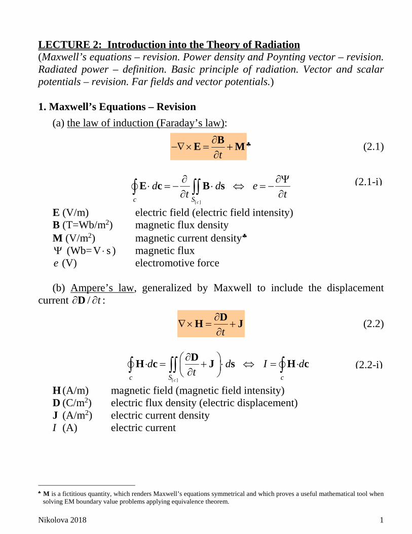
(a) the law of induction (Faraday’s law):

t

∂−∇× = +

∂BE M♣ (2.1)

[ ]cc S

d d et t∂ ∂Ψ

⋅ = − ⋅ ⇔ = −∂ ∂∫ ∫∫E c B s

E (V/m) electric field (electric field intensity) B (T=Wb/m2) magnetic flux density M (V/m2) magnetic current density♣ Ψ (Wb=V s⋅ ) magnetic flux

e (V) electromotive force

(b) Ampere’s law, generalized by Maxwell to include the displacement current / t∂ ∂D :

t

∂∇× = +

∂DH J (2.2)

[ ]cc S c

d d I dt

∂ ⋅ = + ⋅ ⇔ = ⋅ ∂ ∫ ∫∫ ∫DH c J s H c

H (A/m) magnetic field (magnetic field intensity) D (C/m2) electric flux density (electric displacement) J (A/m2) electric current density I (A) electric current

♣ M is a fictitious quantity, which renders Maxwell’s equations symmetrical and which proves a useful mathematical tool when

solving EM boundary value problems applying equivalence theorem.

(2.1-i)

(2.2-i)

Nikolova 2018 2

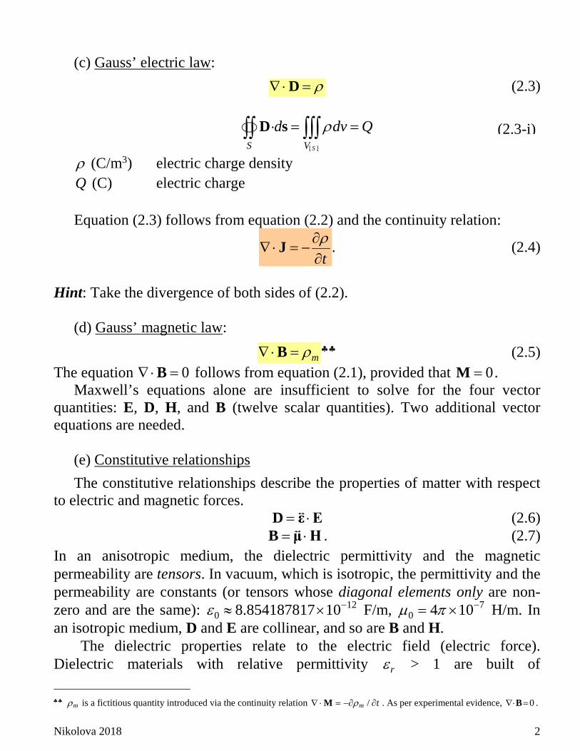
(c) Gauss’ electric law: ρ∇ ⋅ =D (2.3)

[ ]SS V

d dv Qρ⋅ = =∫∫ ∫∫∫D s

ρ (C/m3) electric charge density Q (C) electric charge

Equation (2.3) follows from equation (2.2) and the continuity relation:

tρ∂

∇ ⋅ = −∂

J . (2.4)

Hint: Take the divergence of both sides of (2.2).

(d) Gauss’ magnetic law: mρ∇ ⋅ =B ♣♣ (2.5)

The equation 0∇⋅ =B follows from equation (2.1), provided that 0=M . Maxwell’s equations alone are insufficient to solve for the four vector

quantities: E, D, H, and B (twelve scalar quantities). Two additional vector equations are needed.

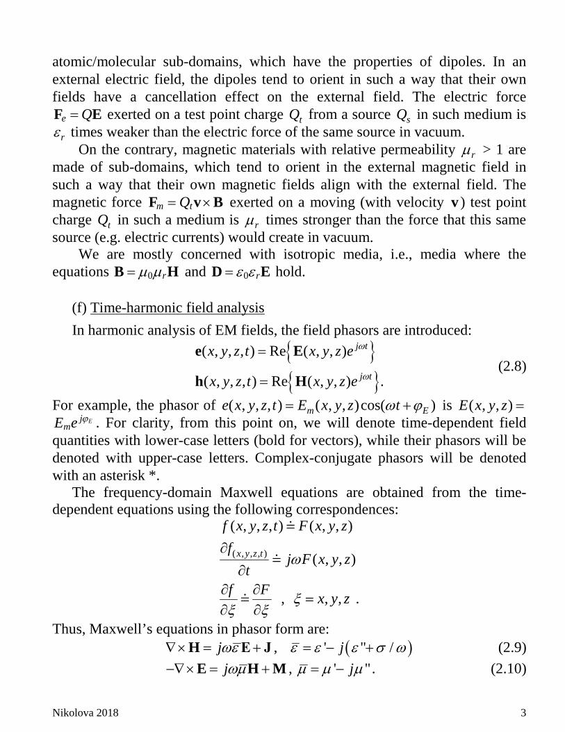
(e) Constitutive relationships The constitutive relationships describe the properties of matter with respect

to electric and magnetic forces. = ⋅D ε E (2.6) = ⋅B μ H . (2.7)

In an anisotropic medium, the dielectric permittivity and the magnetic permeability are tensors. In vacuum, which is isotropic, the permittivity and the permeability are constants (or tensors whose diagonal elements only are non-zero and are the same): 12

0 8.854187817 10ε −≈ × F/m, 70 4 10µ π −= × H/m. In

an isotropic medium, D and E are collinear, and so are B and H. The dielectric properties relate to the electric field (electric force).

Dielectric materials with relative permittivity rε > 1 are built of ♣♣ mρ is a fictitious quantity introduced via the continuity relation /m tρ∇ ⋅ = −∂ ∂M . As per experimental evidence, 0∇⋅ =B .

(2.3-i)

Nikolova 2018 3

atomic/molecular sub-domains, which have the properties of dipoles. In an external electric field, the dipoles tend to orient in such a way that their own fields have a cancellation effect on the external field. The electric force

e Q=F E exerted on a test point charge tQ from a source sQ in such medium is rε times weaker than the electric force of the same source in vacuum.

On the contrary, magnetic materials with relative permeability rµ > 1 are made of sub-domains, which tend to orient in the external magnetic field in such a way that their own magnetic fields align with the external field. The magnetic force m tQ= ×F v B exerted on a moving (with velocity v ) test point charge tQ in such a medium is rµ times stronger than the force that this same source (e.g. electric currents) would create in vacuum.

We are mostly concerned with isotropic media, i.e., media where the equations 0 rµ µ=B H and 0 rε ε=D E hold.

(f) Time-harmonic field analysis In harmonic analysis of EM fields, the field phasors are introduced:

( , , , ) Re ( , , )

( , , , ) Re ( , , ) .

j t

j t

x y z t x y z e

x y z t x y z e

ω

ω

=

=

e E

h H (2.8)

For example, the phasor of ( , , , ) ( , , )cos( )m Ee x y z t E x y z tω ϕ= + is ( , , )E x y z = Ej

mE e ϕ . For clarity, from this point on, we will denote time-dependent field quantities with lower-case letters (bold for vectors), while their phasors will be denoted with upper-case letters. Complex-conjugate phasors will be denoted with an asterisk *.

The frequency-domain Maxwell equations are obtained from the time-dependent equations using the following correspondences:

( , , , )

( , , , ) ( , , )

( , , )

, , , .

x y z t

f x y z t F x y zf

j F x y zt

f F x y z

ω

ξξ ξ

∂∂

∂ ∂=

∂ ∂

Thus, Maxwell’s equations in phasor form are: jωε∇× = +H Ε J , ( )' " /jε ε ε σ ω= − + (2.9)

jωµ−∇× = +E H M , ' "jµ µ µ= − . (2.10)

Nikolova 2018 4

These equations include the equivalent (fictitious) magnetic currents M. The imaginary part of the complex dielectric permittivity ε describes loss. Often, the dielectric loss is represented by the dielectric loss angle dδ :

"' 1 ' 1 tan' ' 'dj jε σ σε ε ε δ

ε ωε ωε = − + = − +

. (2.11)

Similarly, the magnetic loss is described by the imaginary part of the complex magnetic permeability µ or by the magnetic loss angle mδ :

( )"' " ' 1 ' 1 tan' mj j jµµ µ µ µ µ δ

µ

= − = − = −

. (2.12)

In antenna theory, we are mostly concerned with isotropic, homogeneous and loss-free propagation media. 2. Power Density, Poynting Vector, Radiated Power

2.1. Poynting vector – revision In the time-domain analysis, the Poynting vector is defined as

( ) ( ) ( )t t t= ×p e h , W/m2. (2.13) As follows from Poynting’s theorem, p is a vector representing the density and the direction of the EM power flow. Thus, the total power leaving certain volume V is obtained as

[ ]

( ) ( )VS

t t dΠ = ⋅∫∫ p s

, W. (2.14)

Since

( )1( ) Re2

j t j t j tt e e eω ω ω∗ −= = +e E E E , (2.15)

and

( )1( ) Re2

j t j t j tt e e eω ω ω∗ −= = +h H H H , (2.16)

the instantaneous power density appears as

21 1( ) Re Re2 2

av

j tt e ω∗ ⋅= × + × ⋅

p

p E H E H

. (2.17)

The first term in (2.17), avp , has no time dependence. It is the average value, about which the power flux density fluctuates. It is a vector of unchanging direction showing a constant outflow (positive value) or inflow

Nikolova 2018 5

(negative value) of EM power. It describes the active (or time-average) power flow,

[ ]S V

avav dΠ = ⋅∫∫ p s

. (2.18)

The second term in (2.17) is a vector changing its direction with a double frequency 2ω . It describes power flow, which fluctuates in space (propagates to and fro) without contribution to the overall transport of energy. If there is no phase difference between E and H , ( )tp always maintains the same direction (the direction of the outgoing wave) although it changes in intensity. This is because the 2nd term in (2.17) never exceeds in magnitude the first term, i.e.,

avp . This indicates that the power moves away from the source at every instant of time, with the Poynting vector never directed toward the source.

However, if E and H are out of phase ( 0H Eϕ ϕ ϕ∆ = − ≠ ), there are time periods during which the Poynting vector does reverse its direction toward the source and when doing so it achieves a maximum value of 0.5 Im ∗⋅ ×E H .

In fact, the time-dependent Poynting vector can be decomposed into two parts: (i) a real-positive (active) part fluctuating with double frequency about the average value 0.5 Re av

∗= ⋅ ×p E H , i.e., swinging between zero and cosm mE H ϕ∆ , and (ii) a double-frequency part of magnitude 0.5 Im ∗⋅ ×E H ,

which becomes negative every other quarter-period (reactive). You will prove and illustrate this in your next Assignment. Definition: The complex Poynting vector is the vector

12

∗= ×P E H , (2.19)

whose real part is equal to the average power flux density: Reav =p P .

2.2. Radiated power Definition: Radiated power is the average power radiated by the antenna:

[ ] [ ] [ ]

1Re Re2S S SV V V

avrad d d d∗Π = ⋅ ⋅ × ⋅∫∫ ∫∫ ∫∫= =p s P s E H s

. (2.20)

Nikolova 2018 6

3. Basic Principle of Radiation 3.1. Current element

Definition: A current element ( I l∆ ), A m× , is a filament of length l∆ carrying current I. It is sufficiently small to imply constant magnitude of the current along l∆ .

The time-varying current element is the elementary source of EM radiation. It has fundamental significance in radiation theory similar to the fundamental concept of a point charge in electrostatics. The field radiated by a complex antenna in a linear medium can be analyzed using the superposition principle after decomposing the antenna into elementary sources, i.e., current elements.

The time-dependent current density vector j depends on the charge density ρ and its velocity v as

2, A / mρ= ⋅j v . (2.21) If the current flows along a wire of cross-section S∆ , then the product

l Sρ ρ= ⋅∆ [C/m] is the charge per unit length (charge line density) along the wire. Thus, for the current i = ⋅∆j S it follows that

li v ρ= ⋅ , A. (2.22) Then

l ldi dv adt dt

ρ ρ= = ⋅ , A/s, (2.23)

where a (m/s2) is the acceleration of the charge. The time-derivative of a current element i l∆ is then proportional to the amount of charge q enclosed in the volume of the current element and to its acceleration:

, A m/slldi adt

al qρ= ∆ ⋅ ⋅ ×⋅=∆ . (2.24)

3.2. Mathematical description of the accelerated charge as a radiation source It is not immediately obvious from Maxwell’s equations that the time-

varying current is the source of radiation. A simple transformation of the time-dependent Maxwell equations,

Radiation is produced by accelerated or decelerated charge (time-varying current element).

Nikolova 2018 7

,

t

t

µ

ε

∂−∇× =

∂∂

∇× = +∂

he

eh j

(2.25)

into a single second-order equation either for E or for the H field proves this statement. By taking the curl of both sides of the first equation in (2.25) and by making use of the second equation in (2.25), we obtain

2

2 ttµε µ∂ ∂

∇×∇× + = −∂∂

e je . (2.26)

From (2.26), it is obvious that the time derivative of the electric current is the source for the wave-like vector e. Time-constant currents do not radiate.

In an analogous way, one can obtain the wave equation for the magnetic field H and its sources:

2

2tµε ∂∇×∇× + =∇×

∂hh j . (2.27)

Notice that, as follows from (2.27) and (2.25), curl-free currents (e.g., ψ= ∇j ) do not radiate either.

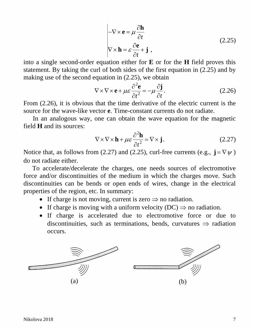
To accelerate/decelerate the charges, one needs sources of electromotive force and/or discontinuities of the medium in which the charges move. Such discontinuities can be bends or open ends of wires, change in the electrical properties of the region, etc. In summary:

• If charge is not moving, current is zero ⇒ no radiation. • If charge is moving with a uniform velocity (DC) ⇒ no radiation. • If charge is accelerated due to electromotive force or due to

discontinuities, such as terminations, bends, curvatures ⇒ radiation occurs.

(a)

(b)

Nikolova 2018 8

(c)

(d)

(e)

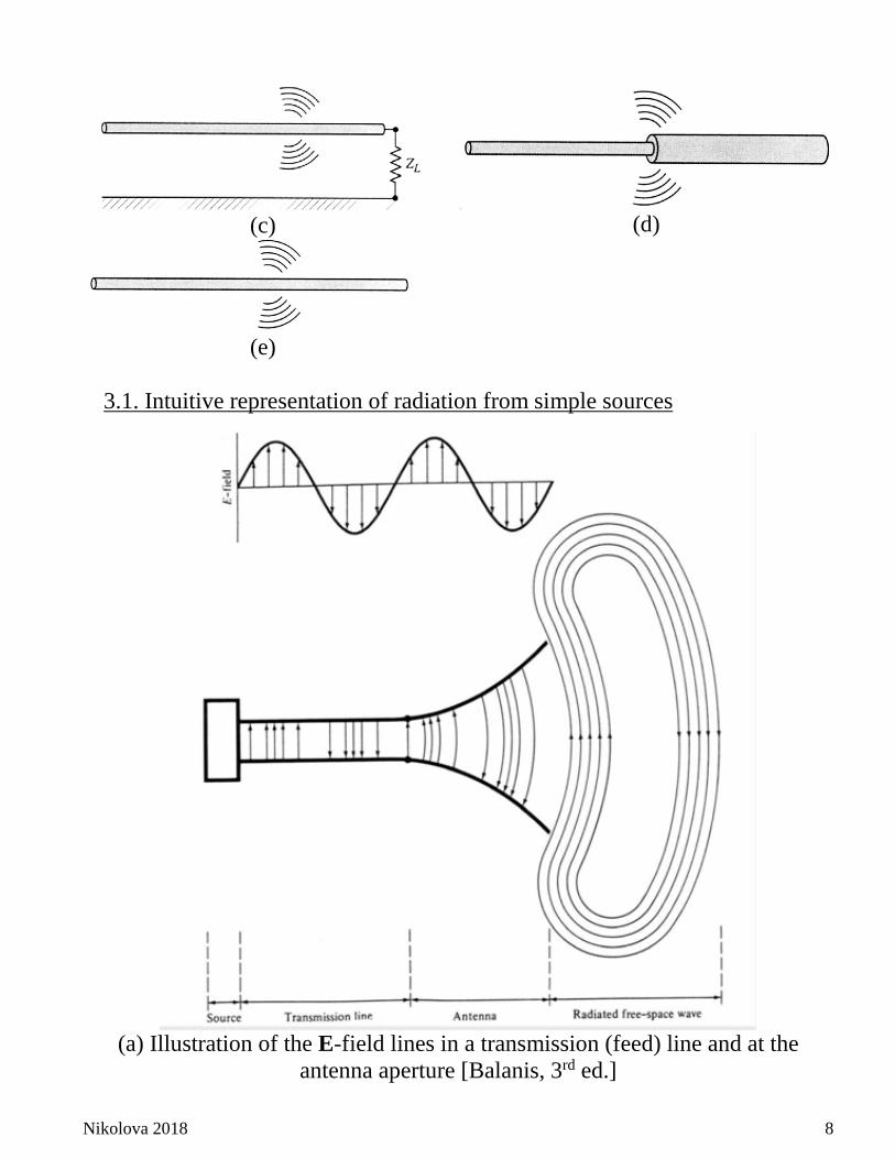
3.1. Intuitive representation of radiation from simple sources

(a) Illustration of the E-field lines in a transmission (feed) line and at the

antenna aperture [Balanis, 3rd ed.]

Nikolova 2018 9

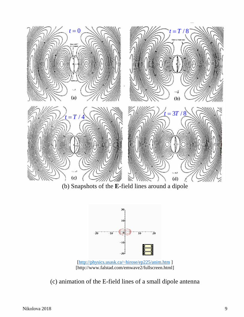
(b) Snapshots of the E-field lines around a dipole

[http://physics.usask.ca/~hirose/ep225/anim.htm ]

[http://www.falstad.com/emwave2/fullscreen.html]

(c) animation of the E-field lines of a small dipole antenna

0t = / 8t T=

/ 4t T= 3 / 8t T=

Nikolova 2018 10

4. Radiation Boundary Condition With few exceptions, antennas are assumed to radiate in open (unbounded)

space. This is a crucial factor determining the field behavior. Often, the EM sources (currents and charges on the antenna) are more or less accurately known. These sources are then assumed to radiate in unbounded space and the resulting EM field is determined as integrals over the currents on the antenna. Such problems, where the field sources are known and the resulting field is to be determined are called analysis (forward, direct) problems.1 To ensure the uniqueness of the solution in an unbounded analysis problem, we have to impose the radiation boundary condition (RBC) on the EM field vectors, i.e., for distances far away from the source (r →∞ ),

ˆ( ) 0,

1 ˆ( ) 0 .

r

r

η

η

− × →

− × →

E H r

H r E (2.28)

The above RBC is known as the Sommerfeld vector RBC or the Silver-Müller RBC. Here, η is the intrinsic impedance of the medium; 0 0/ 377 η µ ε= ≈ Ω in vacuum.

The specifics of the antenna problems lead to the introduction of auxiliary vector potential functions, which allow simpler and more compact solutions.

It is customary to perform the EM analysis for the case of time-harmonic fields, i.e., in terms of phasors. This course adheres to this tradition. Therefore, from now on, all field quantities (vectors and scalars) are to be understood as complex phasor quantities, the absolute values of which correspond to the magnitudes (not the RMS value!) of the respective sine waves. 5. Vector and Scalar Potentials – Review

In radiation theory, the potential functions are almost exclusively in the form of retarded potentials, i.e., the magnetic vector potential A and its scalar counterpart Φ form a 4-potential in space-time and they are related through the Lorenz gauge. We next introduce the retarded potentials.

5.1. The magnetic vector potential A We first consider only electric sources (J and ρ , jωρ∇⋅ = −J ).

1 The inverse (or design) problem is the problem of finding the sources of a known field.

Nikolova 2018 11

,

.j

jωµωε

∇× = −∇× = +

E HH E J

(2.29)

Since 0∇⋅ =B , we can assume that =∇×B A . (2.30)

Substituting (2.30) in (2.29) yields

,

1 .

j

j

ω

ωεµ

= − −∇Φ

= ∇× ∇× −

E A

E A J (2.31)

From (2.31), a single equation can be written for A: ( )j jωµε ω µ∇×∇× + +∇Φ =A A J . (2.32)

Here, Φ denotes the electric scalar potential, which plays an essential role in the analysis of electrostatic fields. To uniquely define A, we need to define not only its curl, but also its divergence. There are no restrictions in defining ∇⋅A . Since 2∇×∇× = ∇∇ ⋅−∇ , equation (2.32) can be simplified by assuming that

jωµε∇ ⋅ = − ΦA . (2.33) Equation (2.33) is known as the Lorenz gauge. It reduces (2.32) to

2 2ω µε µ∇ + = −A A J . (2.34) If the region is lossless, then µ and ε are real numbers, and (2.34) can be written as

2 2β µ∇ + = −A A J , (2.35) where β ω µε= is the phase constant of the medium. If the region is lossy, the complex permittivity ε and the complex permeability µ are introduced. Then, (2.34) becomes

2 2γ µ∇ − = −A A J . (2.36) Here, j jγ α β ω µε= + = is the propagation constant and α is the attenuation constant. 5.2. The electric vector potential F

The magnetic field is a solenoidal field, i.e., 0∇⋅ =B , because there are no physically existing magnetic charges. Therefore, there are no physically existing magnetic currents either. However, the fictitious (equivalent) magnetic currents (density is denoted as M) are a useful tool for antenna analysis when applied with the equivalence principle. These currents are introduced in Maxwell’s equations in a manner dual to that of the electric currents J. Now,

Nikolova 2018 12

we consider the field due to magnetic sources only, i.e., we set 0=J and 0ρ = , and therefore, 0∇⋅ =D . Then, the system of Maxwell’s equations is

,

.j

jωµωε

∇× = − −∇× =

E H MH E

(2.37)

Since D is solenoidal (i.e. 0∇⋅ =D ), it can be expressed as the curl of a vector, namely the electric vector potential F:

= −∇×D F . (2.38) Equation (2.38) is substituted into (2.37). All mathematical transformations are analogous to those made in Section 5.1. Finally, it is shown that a field due to magnetic sources is described by the vector F alone, where F satisfies

2 2ω µε ε∇ + = −F F M (2.39) provided that the Lorenz gauge is imposed as

jωµε∇ ⋅ = − ΨF . (2.40) Here, Ψ is the magnetic scalar potential.

In a linear medium, a field due to both types of sources (magnetic and electric) can be found by superimposing the partial field due to the electric sources only and the one due to the magnetic sources only.

TABLE 2.1: FIELD VECTORS IN TERMS OF VECTOR POTENTIALS Magnetic vector-potential A (electric sources only)

Electric vector-potential F (magnetic sources only)

= ∇×B A , 1µ

= ∇×H A

jjωωµε

= − − ∇∇⋅E A A or

1j jωµε ωε

= ∇×∇× −JE A

= −∇×D F , 1ε

= − ∇×E F

jjωωµε

= − − ∇∇⋅H F F or

1j jωµε ωµ

= ∇×∇× −MH F

6. Retarded Potentials – Review

Retarded potential is a term usually used to denote the solution of the inhomogeneous Helmholtz’ equation (in the frequency domain) or that of the inhomogeneous wave equation (in the time domain) in an unbounded region.

Consider the z-directed electric current density ˆ zJ=J z . According to

Nikolova 2018 13

(2.35), the magnetic vector potential A is also z-directed and is governed by the following equation in a lossless medium:

2 2z z zA A Jβ µ∇ + = − . (2.41)

Eq. (2.41) is a Helmholtz equation and its solution in open space is determined by the integral

[ ]( ) ( , ) ( )Q

z z QV

A P G P Q J Q dvµ= ⋅ −∫∫∫ (2.42)

where ( , )G P Q is the open-space Green’s function of the Helmholtz equation (see the Appendix), P is the observation point, and Q is the source point. Substituting (2.80) from the Appendix into (2.42) gives

( ) ( )4

PQ

Q

j R

z z QPQV

eA P J Q dvR

β

µπ

− = ⋅

∫∫∫ (2.43)

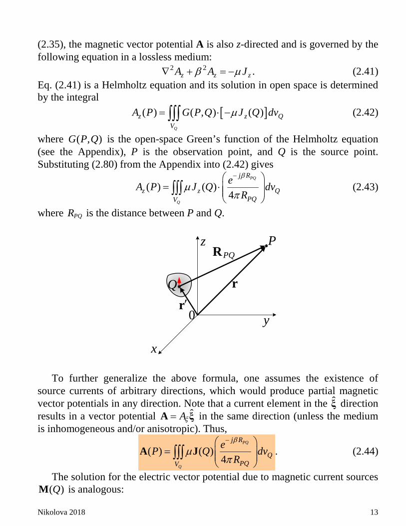
where PQR is the distance between P and Q.

Q

P

0

x

y

zPQR

r′r

To further generalize the above formula, one assumes the existence of

source currents of arbitrary directions, which would produce partial magnetic vector potentials in any direction. Note that a current element in the ξ direction results in a vector potential ˆAξ=A ξ in the same direction (unless the medium is inhomogeneous and/or anisotropic). Thus,

( ) ( )4

PQ

Q

j R

QPQV

eP Q dvR

β

µπ

− =

∫∫∫A J . (2.44)

The solution for the electric vector potential due to magnetic current sources ( )QM is analogous:

Nikolova 2018 14

( ) ( )4

PQ

Q

j R

QPQV

eP Q dvR

β

επ

− =

∫∫∫F M . (2.45)

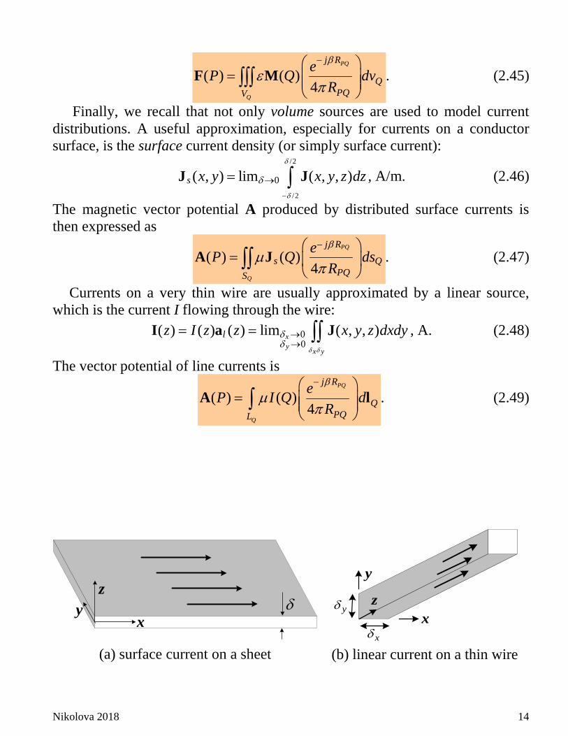
Finally, we recall that not only volume sources are used to model current distributions. A useful approximation, especially for currents on a conductor surface, is the surface current density (or simply surface current):

/2

/2

0( , ) lim ( , , )s x y x y z dzδ

δ

δ−

→= ∫J J , A/m. (2.46)

The magnetic vector potential A produced by distributed surface currents is then expressed as

( ) ( )4

PQ

Q

j R

s QPQS

eP Q dsR

βµ

π

− =

∫∫A J . (2.47)

Currents on a very thin wire are usually approximated by a linear source, which is the current I flowing through the wire:

00

( ) ( ) ( ) lim ( , , )xy

x y

lz I z z x y z dxdyδ δ

δδ

→→

= = ∫∫I a J , A. (2.48)

The vector potential of line currents is

( ) ( )4

PQ

Q

j R

QPQL

eP I Q dR

β

µπ

− =

∫A l . (2.49)

zy

xδ

(a) surface current on a sheet

y

xz

xδ

yδ

(b) linear current on a thin wire

Nikolova 2018 15

7. Far Fields and Vector Potentials 7.1. Potentials Antennas are sources of finite physical dimensions. The further away from

the antenna the observation point is, the more the wave looks like a spherical wave and the more the antenna looks like a point source regardless of its actual shape. For such observation distances, we talk about far field and far zone. The exact meaning of these terms will be discussed later. For now, we will simply accept that the vector potentials behave like spherical waves, when the observation point is far from the source:

dependence on observation angles only dependence on distance only

ˆˆ ˆ( , ) ( , ) ( , ) ,jkr

reA A A r

rθ ϕθ ϕ θ ϕ θ ϕ−

≈ + + ⋅ →∞ A r θ φ

. (2.50)

Here, ˆˆ ˆ( , , )r θ φ are the unit vectors of the spherical coordinate system (SCS) centered on the antenna and k ω µε= is the wave number (or the phase constant). The term jkre− shows propagation along r away from the antenna at the speed of light. The term 1/ r shows the spherical spread of the potential in space, which results in a decrease of its magnitude with distance.

Notice an important feature of the far-field potential: the dependence on the distance r is separable from the dependence on the observation angle ( , )θ ϕ , and it is the same for any antenna: /jkre r− .

Formula (2.50) is a far-field approximation of the vector potential at distant points. We arrive at it starting from the integral in (2.44). When the observation point P is very far from the source, the distance PQR varies only slightly as Q sweeps the volume of the source. It is almost the same as the distance r from the origin (the antenna center) to P. The following first-order approximation (attributed to Kirchhoff) is made for the integrand:

ˆ( )PQjkR jk r

PQ

e eR r

− ′− − ⋅≈

r r. (2.51)

Here, r is the position vector of the observation point P and | |r = r is its length. Its direction is given by the unit vector r , so that ˆ r= ⋅r r . The position vector of the integration point Q is ′r . Equation (2.51) is called the far-field approximation.

The approximation in the phase term (in the exponent) is illustrated in the figures below. The first figure shows the real problem. The second one shows the approximated problem, where, in effect, the vectors PQR and r are parallel.

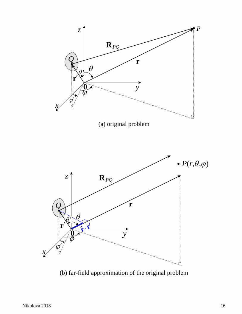
Nikolova 2018 16

r

PQR

z

x

y0

Qθ'θ

ϕ

′r

ϕ′

(a) original problem

′r

z

x

y0

Qθ

ϕϕ′

ˆ ′⋅r r'θ

( , , )P r θ ϕ

r

PQR

(b) far-field approximation of the original problem

P

Nikolova 2018 17

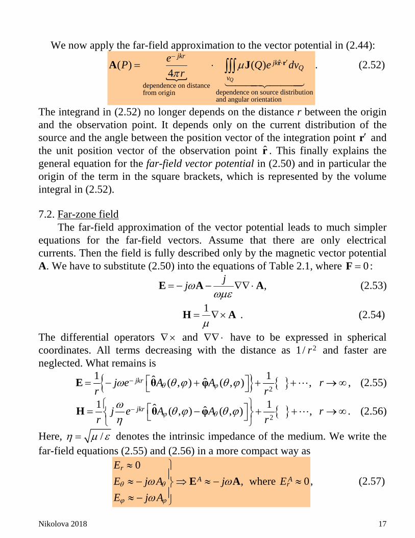
We now apply the far-field approximation to the vector potential in (2.44):

ˆ

dependence on distancedependence on source distributionfrom originand angular orientation

( ) ( )4

Q

jkrjk

Qv

eP Q e dvr

µπ

−′⋅= ⋅ ∫∫∫ r rA J

. (2.52)

The integrand in (2.52) no longer depends on the distance r between the origin and the observation point. It depends only on the current distribution of the source and the angle between the position vector of the integration point ′r and the unit position vector of the observation point r . This finally explains the general equation for the far-field vector potential in (2.50) and in particular the origin of the term in the square brackets, which is represented by the volume integral in (2.52).

7.2. Far-zone field

The far-field approximation of the vector potential leads to much simpler equations for the far-field vectors. Assume that there are only electrical currents. Then the field is fully described only by the magnetic vector potential A. We have to substitute (2.50) into the equations of Table 2.1, where 0=F :

,jjωωµε

= − − ∇∇⋅E A A (2.53)

1 .µ

= ∇×H A (2.54)

The differential operators ∇× and ∇∇ ⋅ have to be expressed in spherical coordinates. All terms decreasing with the distance as 21/ r and faster are neglected. What remains is

2

1 1ˆ ˆ( , ) ( , ) ,jkrj e A A rr rθ ϕω θ ϕ θ ϕ− = − + + + →∞ E θ φ , (2.55)

2

1 1ˆ ˆ( , ) ( , ) ,jkrj e A A rr rϕ θ

ω θ ϕ θ ϕη

− = − + + →∞ H θ φ . (2.56)

Here, /η µ ε= denotes the intrinsic impedance of the medium. We write the far-field equations (2.55) and (2.56) in a more compact way as

0

, where 0r

A Ar

EE j A j EE j Aθ θ

ϕ ϕ

ω ωω

≈ ≈ − ⇒ ≈ − ≈≈ −

E A , (2.57)

Nikolova 2018 18

01ˆ ˆ

r

A A

HE

H j A j

EH j A

ϕθ ϕ

θϕ θ

ω ωη η η ηωη η

≈ ≈ + = − ⇒ ≈ − × = ×

≈ − = +

H r A r E . (2.58)

In an analogous manner, we obtain the relations between the field vectors and the electric vector potential F, when only magnetic sources are present:

0

, 0r

F Fr

HH j F j HH j F

θ θ

ϕ ϕ

ω ωω

≈ ≈ − ⇒ ≈ − ≈≈ −

H F , (2.59)

0

ˆ ˆr

F F

EE j F H jE j F Hθ ϕ ϕ

ϕ θ θ

ωη η ωη ηωη η

≈≈ − = ⇒ ≈ × = − ×≈ + = −

E r F r Η . (2.60)

In summary, the far field of any antenna has the following important features, which follow from equations (2.57) through (2.60): • The far field has negligible radial components, 0rE ≈ and 0rH ≈ . Since

the radial direction is also the direction of propagation, the far field is a typical TEM (Transverse Electro-Magnetic) wave.

• The far-field E vector and H vector are mutually orthogonal, both of them being also orthogonal to the direction of propagation.

• The magnitudes of the electric field and the magnetic field are related always as | | | |η=E H .

Nikolova 2018 19

APPENDIX Green’s Function for the Helmholtz Equation

Suppose the following PDE must be solved: ( ) ( )L fΦ =x x (2.61)

where x denotes the set of variables, e.g., ( , , )x y z=x . Suppose also that a Green’s function exists such that it allows for the integral solution

( ) ( , ) ( )V

G f dv′

′ ′ ′Φ = ⋅∫∫∫x x x x . (2.62)

Applying the operator L to both sides of (2.62), leads to [ ]( ) ( , ) ( ) ( )

V

L LG f dv f′

′ ′ ′Φ = ⋅ =∫∫∫x x x x x . (2.63)

Note that L operates on the variable x while the integral in (2.63) is over ′x . This allows for the insertion of L inside the integral. From (2.63), we conclude that the Green’s function must satisfy the same PDE as Φ with a point source described by Dirac’s delta function:

( , ) ( )LG δ′ ′= −x x x x . (2.64) Here, ( )δ ′−x x is Dirac’s delta function in 3-D space, e.g., ( ) ( ) ( ) ( )x x y y z zδ δ δ δ′ ′ ′ ′− = − − −x x . If the Green’s function of a problem is known and the source function ( )f x is known, the construction of an integral solution is possible via (2.62).

Consider the Green’s function for the Helmholtz equation in open space. It must satisfy 2 2 ( ) ( ) ( )G G x y zβ δ δ δ∇ + = (2.65)

together with the scalar radiation condition

lim 0r

Gr j Gr

β→∞

∂ ⋅ + = ∂ (2.66)

if the source is centered at the origin of the coordinate system, i.e., 0x y z′ ′ ′= = = . Integrate (2.65) within a sphere with its center at (0,0,0) and a radius R:

2 2 1V V

Gdv Gdvβ∇ + =∫∫∫ ∫∫∫ (2.67)

The function G is due to a point source and thus has a spherical symmetry, i.e., it depends on r only.

The Laplacian 2∇ in spherical coordinates is reduced to derivatives with respect to r only:

2

22

2 ( ) ( ) ( )d G dG G x y zr drdr

β δ δ δ+ + = . (2.68)

Everywhere except at the point ( , , )x y z , G must satisfy the homogeneous equation

2

22

2 0d G dG Gr drdr

β+ + = (2.69)

whose solution for outgoing waves is well known:

( )jkreG r C

r

−

= . (2.70)

Here, C is a constant to be determined. Consider first the integral from (2.67): 2

1V

I Gdvβ= ∫∫∫ . (2.71)

R V [S]

Nikolova 2018 20

2

0 0 0

2 2 21 sin

Rj r j r

v

e eI C dv C r d d drr r

π πβ β

β β θ θ ϕ− −

⇒ = =∫∫∫ ∫ ∫ ∫ (2.72)

11( ) 4

j Rj R eI R j C R e

j j

ββπβ

β β

−−

⇒ = ⋅ + −

. (2.73)

To evaluate the integral in the point of singularity (0,0,0), we let 0R → , i.e., we let the sphere collapse into a point. We see that

0 1lim ( ) 0R I R→ = . (2.74) Secondly, consider the other integral in (2.67), ( )2

2V V S

I Gdv G dv G d= ∇ = ∇⋅ ∇ = ∇ ⋅∫∫∫ ∫∫∫ ∫∫ s

. (2.75)

Here, 2 ˆsind R drd dθ θ ϕ= ⋅s r is a surface element on S, and

2ˆ ˆjkr jkrG e eG C jk

r r r

− − ∂∇ = = − + ∂

r r . (2.76)

Substitute (2.76) in (2.75) and carry out the integration over the spherical surface:

( )2

0 0

2( ) sinjkR jkRI R C jkR e e d dπ π

θ ϕ θ− −= − ⋅ + ∫ ∫ (2.77)

0 2lim ( ) 4R I R Cπ→ = − . (2.78) Substituting (2.78) and (2.74) into (2.67) and taking 0limR→ , yields

14

Cπ

= − . (2.79)

Finally,

( )4

jkreG rrπ

−

= − . (2.80)

It is not difficult to show that in the general case when the source is at a point ( , , )Q x y z′ ′ ′ ,

2 2 ( ) ( ) ( )G G x x y y z zβ δ δ δ′ ′ ′∇ + = − − − (2.81) the Green function is

( , )4

PQjkR

PQ

eG P QRπ

−

= − , (2.82)

where PQR is the distance between the observation point P and the source point Q,

2 2 2( ) ( ) ( )PQR x x y y z z′ ′ ′= − + − + − . (2.83)