Embed Size (px)
Citation preview
Lecture 4: 𝐿𝑈 Decomposition and MatrixInverse
Thang Huynh, UC San Diego1/17/2018
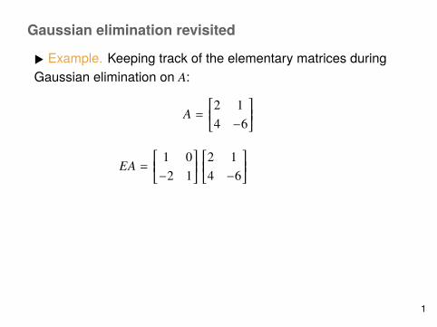
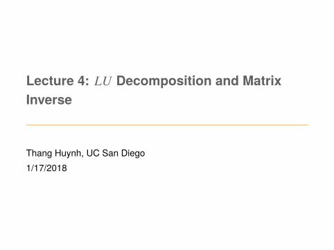
Gaussian elimination revisited
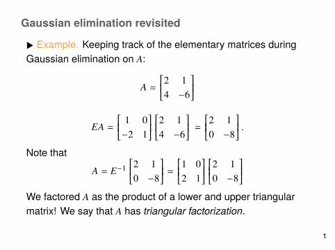
▶ Example. Keeping track of the elementary matrices duringGaussian elimination on 𝐴:
𝐴 = ⎡⎢⎣2 14 −6
⎤⎥⎦
𝐸𝐴 = ⎡⎢⎣
1 0−2 1
⎤⎥⎦
⎡⎢⎣2 14 −6
⎤⎥⎦
= ⎡⎢⎣2 10 −8
⎤⎥⎦
.
Note that𝐴 = 𝐸−1 ⎡⎢
⎣2 10 −8
⎤⎥⎦
= ⎡⎢⎣1 02 1
⎤⎥⎦
⎡⎢⎣2 10 −8
⎤⎥⎦
We factored 𝐴 as the product of a lower and upper triangularmatrix! We say that 𝐴 has triangular factorization.
1

Gaussian elimination revisited
▶ Example. Keeping track of the elementary matrices duringGaussian elimination on 𝐴:
𝐴 = ⎡⎢⎣2 14 −6
⎤⎥⎦
𝐸𝐴 = ⎡⎢⎣
1 0−2 1
⎤⎥⎦
⎡⎢⎣2 14 −6
⎤⎥⎦
= ⎡⎢⎣2 10 −8
⎤⎥⎦
.
Note that𝐴 = 𝐸−1 ⎡⎢
⎣2 10 −8
⎤⎥⎦
= ⎡⎢⎣1 02 1
⎤⎥⎦
⎡⎢⎣2 10 −8
⎤⎥⎦
We factored 𝐴 as the product of a lower and upper triangularmatrix! We say that 𝐴 has triangular factorization.
1

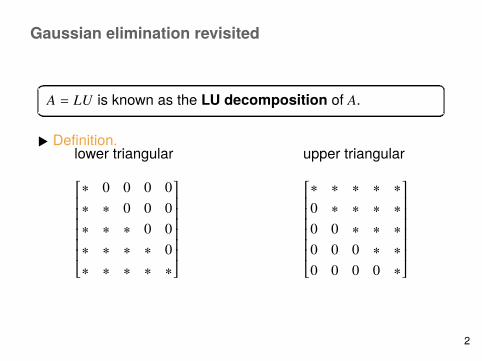
Gaussian elimination revisited
𝐴 = 𝐿𝑈 is known as the LU decomposition of 𝐴.
▶ Definition.lower triangular
⎡⎢⎢⎢⎢⎢⎢⎣
∗ 0 0 0 0∗ ∗ 0 0 0∗ ∗ ∗ 0 0∗ ∗ ∗ ∗ 0∗ ∗ ∗ ∗ ∗
⎤⎥⎥⎥⎥⎥⎥⎦
upper triangular
⎡⎢⎢⎢⎢⎢⎢⎣
∗ ∗ ∗ ∗ ∗0 ∗ ∗ ∗ ∗0 0 ∗ ∗ ∗0 0 0 ∗ ∗0 0 0 0 ∗
⎤⎥⎥⎥⎥⎥⎥⎦
2
Gaussian elimination revisited
𝐴 = 𝐿𝑈 is known as the LU decomposition of 𝐴.
▶ Definition.lower triangular
⎡⎢⎢⎢⎢⎢⎢⎣
∗ 0 0 0 0∗ ∗ 0 0 0∗ ∗ ∗ 0 0∗ ∗ ∗ ∗ 0∗ ∗ ∗ ∗ ∗
⎤⎥⎥⎥⎥⎥⎥⎦
upper triangular
⎡⎢⎢⎢⎢⎢⎢⎣
∗ ∗ ∗ ∗ ∗0 ∗ ∗ ∗ ∗0 0 ∗ ∗ ∗0 0 0 ∗ ∗0 0 0 0 ∗
⎤⎥⎥⎥⎥⎥⎥⎦
2
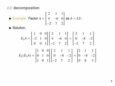
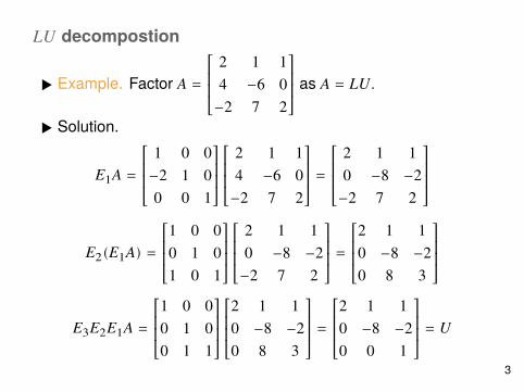
𝐿𝑈 decompostion
▶ Example. Factor 𝐴 =⎡⎢⎢⎣
2 1 14 −6 0
−2 7 2
⎤⎥⎥⎦
as 𝐴 = 𝐿𝑈.
▶ Solution.
𝐸1𝐴 =⎡⎢⎢⎣
1 0 0−2 1 00 0 1
⎤⎥⎥⎦
⎡⎢⎢⎣
2 1 14 −6 0
−2 7 2
⎤⎥⎥⎦
=⎡⎢⎢⎣
2 1 10 −8 −2
−2 7 2
⎤⎥⎥⎦
𝐸2(𝐸1𝐴) =⎡⎢⎢⎣
1 0 00 1 01 0 1
⎤⎥⎥⎦
⎡⎢⎢⎣
2 1 10 −8 −2
−2 7 2
⎤⎥⎥⎦
=⎡⎢⎢⎣
2 1 10 −8 −20 8 3
⎤⎥⎥⎦
𝐸3𝐸2𝐸1𝐴 =⎡⎢⎢⎣
1 0 00 1 00 1 1
⎤⎥⎥⎦
⎡⎢⎢⎣
2 1 10 −8 −20 8 3
⎤⎥⎥⎦
=⎡⎢⎢⎣
2 1 10 −8 −20 0 1
⎤⎥⎥⎦
= 𝑈
3
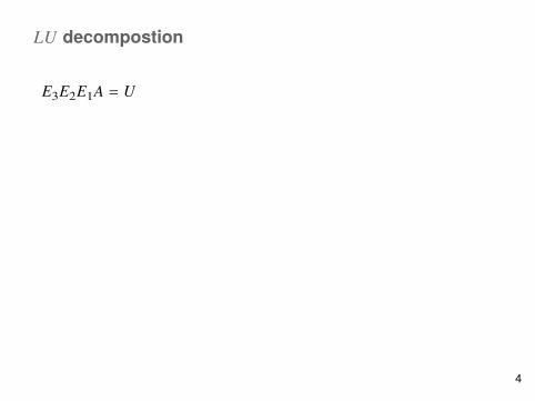
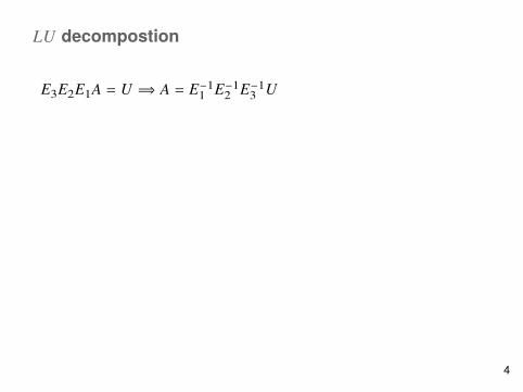
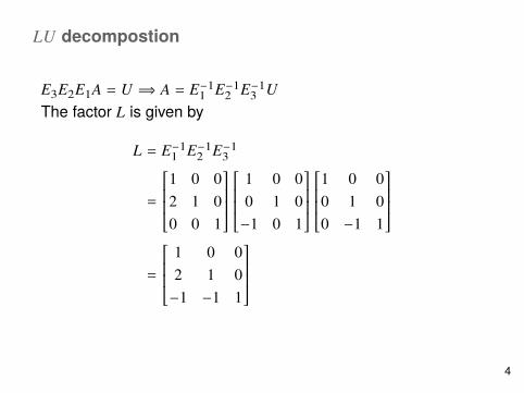
𝐿𝑈 decompostion
𝐸3𝐸2𝐸1𝐴 = 𝑈
⟹ 𝐴 = 𝐸−11 𝐸−1
2 𝐸−13 𝑈
The factor 𝐿 is given by
𝐿 = 𝐸−11 𝐸−1
2 𝐸−13
=⎡⎢⎢⎣
1 0 02 1 00 0 1
⎤⎥⎥⎦
⎡⎢⎢⎣
1 0 00 1 0
−1 0 1
⎤⎥⎥⎦
⎡⎢⎢⎣
1 0 00 1 00 −1 1
⎤⎥⎥⎦
=⎡⎢⎢⎣
1 0 02 1 0
−1 −1 1
⎤⎥⎥⎦
4
𝐿𝑈 decompostion
𝐸3𝐸2𝐸1𝐴 = 𝑈 ⟹ 𝐴 = 𝐸−11 𝐸−1
2 𝐸−13 𝑈
The factor 𝐿 is given by
𝐿 = 𝐸−11 𝐸−1
2 𝐸−13
=⎡⎢⎢⎣
1 0 02 1 00 0 1
⎤⎥⎥⎦
⎡⎢⎢⎣
1 0 00 1 0
−1 0 1
⎤⎥⎥⎦
⎡⎢⎢⎣
1 0 00 1 00 −1 1
⎤⎥⎥⎦
=⎡⎢⎢⎣
1 0 02 1 0
−1 −1 1
⎤⎥⎥⎦
4
𝐿𝑈 decompostion
𝐸3𝐸2𝐸1𝐴 = 𝑈 ⟹ 𝐴 = 𝐸−11 𝐸−1
2 𝐸−13 𝑈
The factor 𝐿 is given by
𝐿 = 𝐸−11 𝐸−1
2 𝐸−13
=⎡⎢⎢⎣
1 0 02 1 00 0 1
⎤⎥⎥⎦
⎡⎢⎢⎣
1 0 00 1 0
−1 0 1
⎤⎥⎥⎦
⎡⎢⎢⎣
1 0 00 1 00 −1 1
⎤⎥⎥⎦
=⎡⎢⎢⎣
1 0 02 1 0
−1 −1 1
⎤⎥⎥⎦
4
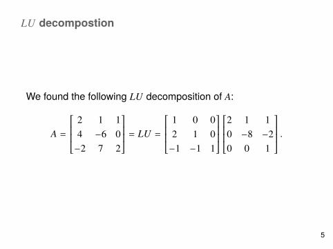
𝐿𝑈 decompostion
We found the following 𝐿𝑈 decomposition of 𝐴:
𝐴 =⎡⎢⎢⎣
2 1 14 −6 0
−2 7 2
⎤⎥⎥⎦
= 𝐿𝑈 =⎡⎢⎢⎣
1 0 02 1 0
−1 −1 1
⎤⎥⎥⎦
⎡⎢⎢⎣
2 1 10 −8 −20 0 1
⎤⎥⎥⎦
.
5
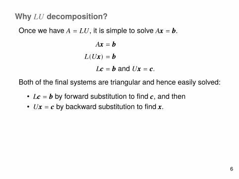
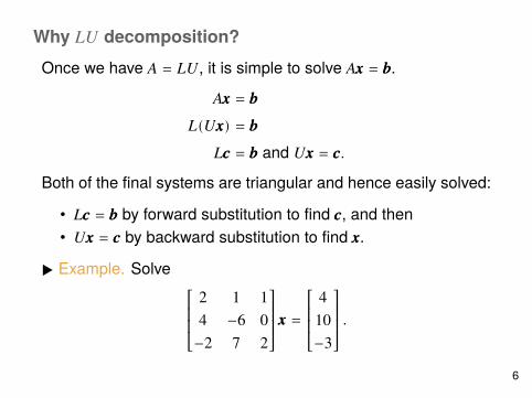
Why 𝐿𝑈 decomposition?Once we have 𝐴 = 𝐿𝑈, it is simple to solve 𝐴𝑥𝑥𝑥 = 𝑏𝑏𝑏.
𝐴𝑥𝑥𝑥 = 𝑏𝑏𝑏𝐿(𝑈𝑥𝑥𝑥) = 𝑏𝑏𝑏
𝐿𝑐𝑐𝑐 = 𝑏𝑏𝑏 and 𝑈𝑥𝑥𝑥 = 𝑐𝑐𝑐.Both of the final systems are triangular and hence easily solved:
• 𝐿𝑐𝑐𝑐 = 𝑏𝑏𝑏 by forward substitution to find 𝑐𝑐𝑐, and then• 𝑈𝑥𝑥𝑥 = 𝑐𝑐𝑐 by backward substitution to find 𝑥𝑥𝑥.
▶ Example. Solve
⎡⎢⎢⎣
2 1 14 −6 0
−2 7 2
⎤⎥⎥⎦
𝑥𝑥𝑥 =⎡⎢⎢⎣
410−3
⎤⎥⎥⎦
.
6

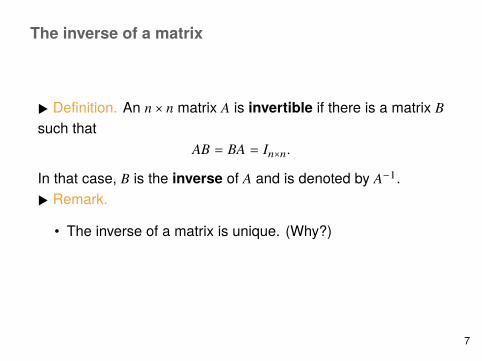
The inverse of a matrix
▶ Definition. An 𝑛 × 𝑛 matrix 𝐴 is invertible if there is a matrix 𝐵such that
𝐴𝐵 = 𝐵𝐴 = 𝐼𝑛×𝑛.
In that case, 𝐵 is the inverse of 𝐴 and is denoted by 𝐴−1.
▶ Remark.
• The inverse of a matrix is unique. (Why?)• Do not write 𝐴
𝐵 .
7
The inverse of a matrix
▶ Definition. An 𝑛 × 𝑛 matrix 𝐴 is invertible if there is a matrix 𝐵such that
𝐴𝐵 = 𝐵𝐴 = 𝐼𝑛×𝑛.
In that case, 𝐵 is the inverse of 𝐴 and is denoted by 𝐴−1.▶ Remark.
• The inverse of a matrix is unique. (Why?)
• Do not write 𝐴𝐵 .
7

The inverse of a matrix
▶ Definition. An 𝑛 × 𝑛 matrix 𝐴 is invertible if there is a matrix 𝐵such that
𝐴𝐵 = 𝐵𝐴 = 𝐼𝑛×𝑛.
In that case, 𝐵 is the inverse of 𝐴 and is denoted by 𝐴−1.▶ Remark.
• The inverse of a matrix is unique. (Why?)• Do not write 𝐴
𝐵 .
7
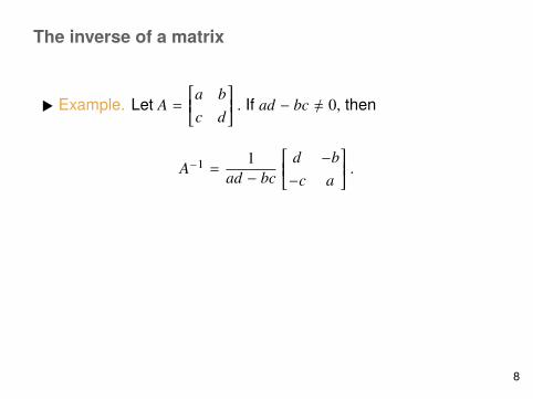
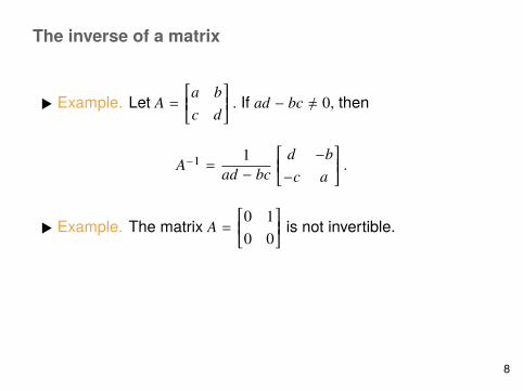
The inverse of a matrix
▶ Example. Let 𝐴 = ⎡⎢⎣𝑎 𝑏𝑐 𝑑
⎤⎥⎦
. If 𝑎𝑑 − 𝑏𝑐 ≠ 0, then
𝐴−1 = 1𝑎𝑑 − 𝑏𝑐
⎡⎢⎣
𝑑 −𝑏−𝑐 𝑎
⎤⎥⎦
.
▶ Example. The matrix 𝐴 = ⎡⎢⎣0 10 0
⎤⎥⎦
is not invertible.
▶ Example. A 2 × 2 matrix ⎡⎢⎣𝑎 𝑏𝑐 𝑑
⎤⎥⎦
is invertible if and only if
𝑎𝑑 − 𝑏𝑐 ≠ 0.
8
The inverse of a matrix
▶ Example. Let 𝐴 = ⎡⎢⎣𝑎 𝑏𝑐 𝑑
⎤⎥⎦
. If 𝑎𝑑 − 𝑏𝑐 ≠ 0, then
𝐴−1 = 1𝑎𝑑 − 𝑏𝑐
⎡⎢⎣
𝑑 −𝑏−𝑐 𝑎
⎤⎥⎦
.
▶ Example. The matrix 𝐴 = ⎡⎢⎣0 10 0
⎤⎥⎦
is not invertible.
▶ Example. A 2 × 2 matrix ⎡⎢⎣𝑎 𝑏𝑐 𝑑
⎤⎥⎦
is invertible if and only if
𝑎𝑑 − 𝑏𝑐 ≠ 0.
8

The inverse of a matrix
▶ Example. Let 𝐴 = ⎡⎢⎣𝑎 𝑏𝑐 𝑑
⎤⎥⎦
. If 𝑎𝑑 − 𝑏𝑐 ≠ 0, then
𝐴−1 = 1𝑎𝑑 − 𝑏𝑐
⎡⎢⎣
𝑑 −𝑏−𝑐 𝑎
⎤⎥⎦
.
▶ Example. The matrix 𝐴 = ⎡⎢⎣0 10 0
⎤⎥⎦
is not invertible.
▶ Example. A 2 × 2 matrix ⎡⎢⎣𝑎 𝑏𝑐 𝑑
⎤⎥⎦
is invertible if and only if
𝑎𝑑 − 𝑏𝑐 ≠ 0.
8
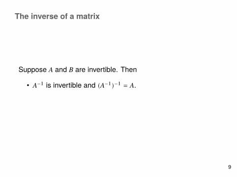
The inverse of a matrix
Suppose 𝐴 and 𝐵 are invertible. Then
• 𝐴−1 is invertible and (𝐴−1)−1 = 𝐴.
• 𝐴𝑇 is invertible and (𝐴𝑇 )−1 = (𝐴−1)𝑇 .• 𝐴𝐵 is invertible and (𝐴𝐵)−1 = 𝐵−1𝐴−1. (Why?)
9
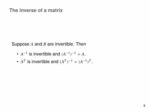
The inverse of a matrix
Suppose 𝐴 and 𝐵 are invertible. Then
• 𝐴−1 is invertible and (𝐴−1)−1 = 𝐴.• 𝐴𝑇 is invertible and (𝐴𝑇 )−1 = (𝐴−1)𝑇 .
• 𝐴𝐵 is invertible and (𝐴𝐵)−1 = 𝐵−1𝐴−1. (Why?)
9
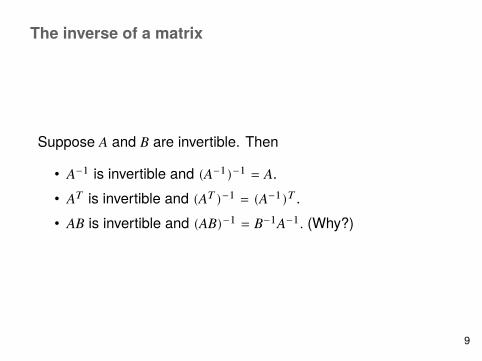
The inverse of a matrix
Suppose 𝐴 and 𝐵 are invertible. Then
• 𝐴−1 is invertible and (𝐴−1)−1 = 𝐴.• 𝐴𝑇 is invertible and (𝐴𝑇 )−1 = (𝐴−1)𝑇 .• 𝐴𝐵 is invertible and (𝐴𝐵)−1 = 𝐵−1𝐴−1. (Why?)
9
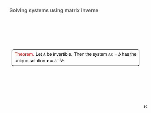
Solving systems using matrix inverse
Theorem. Let 𝐴 be invertible. Then the system 𝐴𝑥𝑥𝑥 = 𝑏𝑏𝑏 has theunique solution 𝑥𝑥𝑥 = 𝐴−1𝑏𝑏𝑏.
10
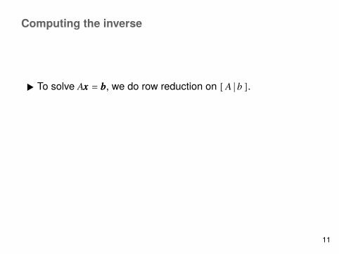
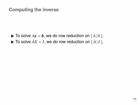
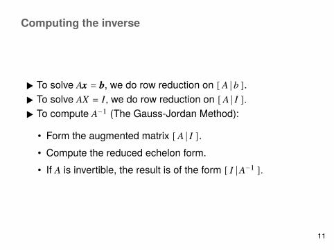
Computing the inverse
▶ To solve 𝐴𝑥𝑥𝑥 = 𝑏𝑏𝑏, we do row reduction on [ 𝐴 ∣ 𝑏 ].
▶ To solve 𝐴𝑋 = 𝐼, we do row reduction on [ 𝐴 ∣ 𝐼 ].▶ To compute 𝐴−1 (The Gauss-Jordan Method):
• Form the augmented matrix [ 𝐴 ∣ 𝐼 ].• Compute the reduced echelon form.• If 𝐴 is invertible, the result is of the form [ 𝐼 ∣ 𝐴−1 ].
11
Computing the inverse
▶ To solve 𝐴𝑥𝑥𝑥 = 𝑏𝑏𝑏, we do row reduction on [ 𝐴 ∣ 𝑏 ].▶ To solve 𝐴𝑋 = 𝐼, we do row reduction on [ 𝐴 ∣ 𝐼 ].
▶ To compute 𝐴−1 (The Gauss-Jordan Method):
• Form the augmented matrix [ 𝐴 ∣ 𝐼 ].• Compute the reduced echelon form.• If 𝐴 is invertible, the result is of the form [ 𝐼 ∣ 𝐴−1 ].
11
Computing the inverse
▶ To solve 𝐴𝑥𝑥𝑥 = 𝑏𝑏𝑏, we do row reduction on [ 𝐴 ∣ 𝑏 ].▶ To solve 𝐴𝑋 = 𝐼, we do row reduction on [ 𝐴 ∣ 𝐼 ].▶ To compute 𝐴−1 (The Gauss-Jordan Method):
• Form the augmented matrix [ 𝐴 ∣ 𝐼 ].• Compute the reduced echelon form.• If 𝐴 is invertible, the result is of the form [ 𝐼 ∣ 𝐴−1 ].
11
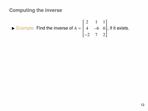
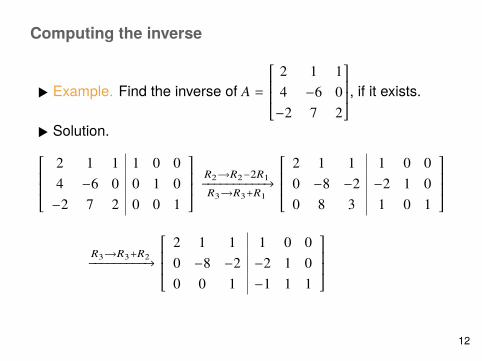
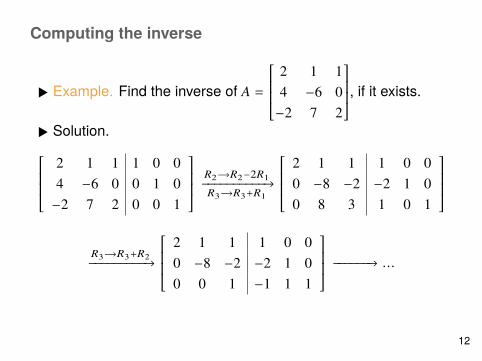
Computing the inverse
▶ Example. Find the inverse of 𝐴 =⎡⎢⎢⎣
2 1 14 −6 0
−2 7 2
⎤⎥⎥⎦, if it exists.
▶ Solution.
⎡⎢⎢⎣
2 1 1 1 0 04 −6 0 0 1 0
−2 7 2 0 0 1
⎤⎥⎥⎦
𝑅2⟶𝑅2−2𝑅1−−−−−−−−−−→𝑅3⟶𝑅3+𝑅1
⎡⎢⎢⎣
2 1 1 1 0 00 −8 −2 −2 1 00 8 3 1 0 1
⎤⎥⎥⎦
𝑅3⟶𝑅3+𝑅2−−−−−−−−−→⎡⎢⎢⎣
2 1 1 1 0 00 −8 −2 −2 1 00 0 1 −1 1 1
⎤⎥⎥⎦
−−−−−−→ …
12

Computing the inverse
−−−−−−→⎡⎢⎢⎣
1 0 0 1216
−516
−616
0 1 0 48
−38
−28
0 0 1 −1 1 1
⎤⎥⎥⎦
𝐴−1 =⎡⎢⎢⎣
1216
−516
−616
48
−38
−28
−1 1 1
⎤⎥⎥⎦
13
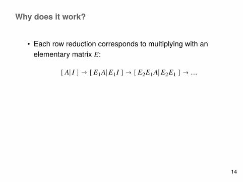
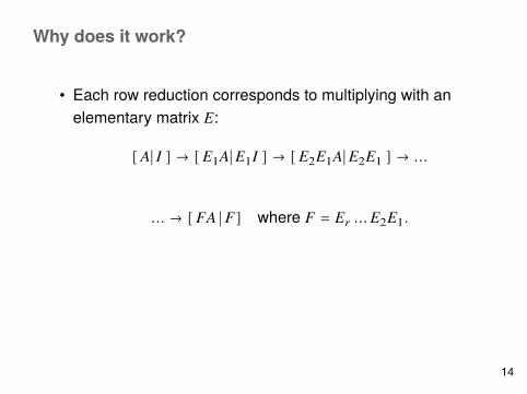
Why does it work?
• Each row reduction corresponds to multiplying with anelementary matrix 𝐸:
[ 𝐴∣ 𝐼 ] → [ 𝐸1𝐴∣ 𝐸1𝐼 ] → [ 𝐸2𝐸1𝐴∣ 𝐸2𝐸1 ] → …
… → [ 𝐹𝐴 ∣ 𝐹] where 𝐹 = 𝐸𝑟 … 𝐸2𝐸1.
• If we manage to reduce [ 𝐴∣ 𝐼 ] to [ 𝐼∣ 𝐹 ], this means
𝐹𝐴 = 𝐼 ⟹ 𝐴−1 = 𝐹.
14
Why does it work?
• Each row reduction corresponds to multiplying with anelementary matrix 𝐸:
[ 𝐴∣ 𝐼 ] → [ 𝐸1𝐴∣ 𝐸1𝐼 ] → [ 𝐸2𝐸1𝐴∣ 𝐸2𝐸1 ] → …
… → [ 𝐹𝐴 ∣ 𝐹] where 𝐹 = 𝐸𝑟 … 𝐸2𝐸1.
• If we manage to reduce [ 𝐴∣ 𝐼 ] to [ 𝐼∣ 𝐹 ], this means
𝐹𝐴 = 𝐼 ⟹ 𝐴−1 = 𝐹.
14
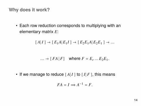
Why does it work?
• Each row reduction corresponds to multiplying with anelementary matrix 𝐸:
[ 𝐴∣ 𝐼 ] → [ 𝐸1𝐴∣ 𝐸1𝐼 ] → [ 𝐸2𝐸1𝐴∣ 𝐸2𝐸1 ] → …
… → [ 𝐹𝐴 ∣ 𝐹] where 𝐹 = 𝐸𝑟 … 𝐸2𝐸1.
• If we manage to reduce [ 𝐴∣ 𝐼 ] to [ 𝐼∣ 𝐹 ], this means
𝐹𝐴 = 𝐼 ⟹ 𝐴−1 = 𝐹.
14