Lesson 1 NXT SegWay Robot - 3D CAD Design … Left and right side of the rider bottom. 7 Arms and chest. 8 Rider’s head. Left side Right side Left side Right side SolidWorks NXT

SolidWorksEngineering Design and Technology Series

1

Lesson 1NXT SegWay Robot

When you complete this lesson, you will be able to:

Setup a motion simulation; User functions and expressions; Create basic control system.

SolidWorks NXT SegWay RobotEngineering Design and Technology Series

Project Description 2

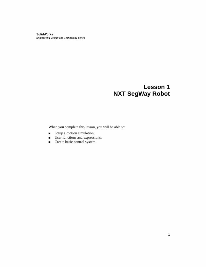
SegWay TransportationSegWay Personal Transporter (PT) is the World’s first self balancing transportation device with two wheels. The mechanism is based on the principle of inverted pendulum with advanced control to maintain balance at all times. To move, rider leans forward or backward and the transporter accelerates in the proper direction to balance the system. Similarly, to take turns the rider leans sideways and the transporter adjusts the speed of both weels. Handling feels natural because the amount of lean, measured by gyroscope, controls the acceleration and the curvature of turns.

Project DescriptionIn this project, you will simulate the SegWay robot built using the Lego Mindstorms NXT 2.0 kit. In the first part of the lesson, you will create a system control in SolidWorks Motion and compare it to the behavior of the robot. You will consider two scenarios.

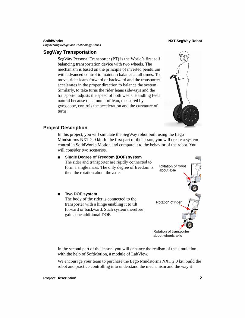
Single Degree of Freedom (DOF) systemThe rider and transporter are rigidly connected to form a single mass. The only degree of freedom is then the rotation about the axle.

Two DOF systemThe body of the rider is connected to the transporter with a hinge enabling it to tilt forward or backward. Such system therefore gains one additional DOF.

In the second part of the lesson, you will enhance the realism of the simulation with the help of SoftMotion, a module of LabView.

We encourage your team to purchase the Lego Mindstorms NXT 2.0 kit, build the robot and practice controlling it to understand the mechanism and the way it

Rotation of robot about axle

Rotation of transporter about wheels axle

Rotation of rider


Simulation with SolidWorks 3

works. The differencies between simulation in SolidWorks Motion and the real behavior will then be better understood. The behavior of robot under various cirmustances can be viewed in video files supplied with the project and at http://www.nxtprograms.com/NXT2/segway/.

Lego Mindstorms NXT 2.0 Robot

Follow the instructions at http://www.nxtprograms.com/NXT2/segway/index.html and build your own robot. Then, experiment with two control programs, SegWay and Segway BT, supplied on the website.

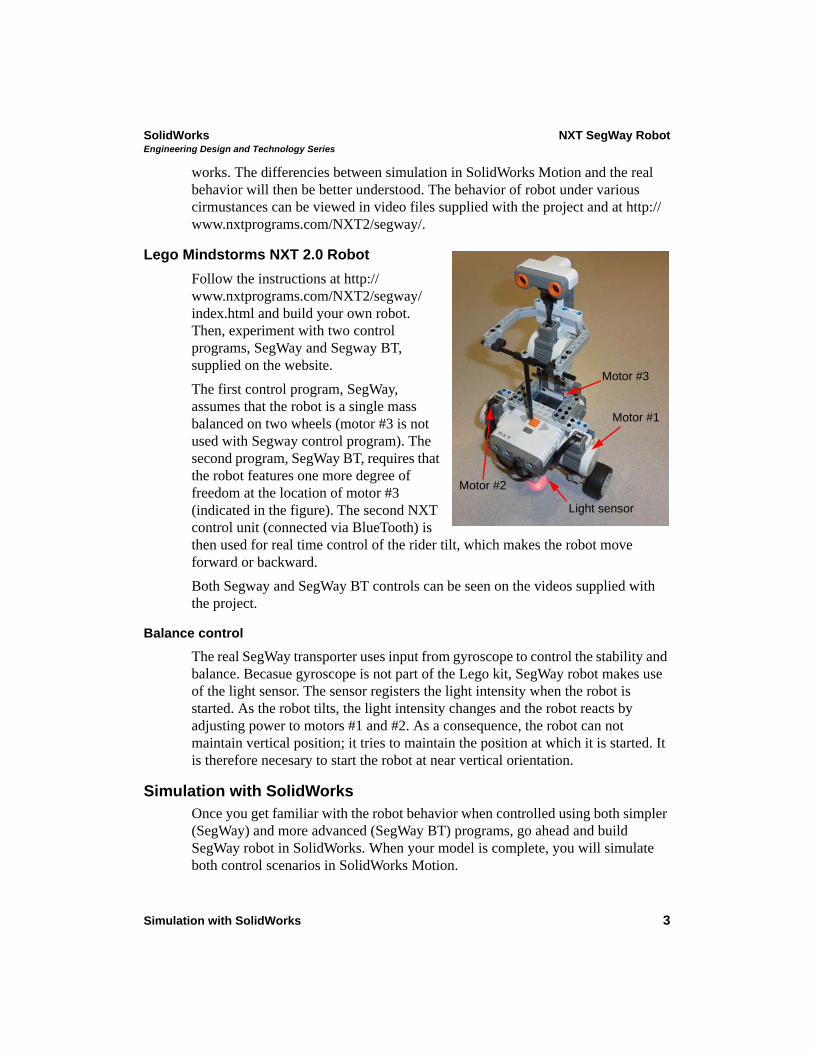
The first control program, SegWay, assumes that the robot is a single mass balanced on two wheels (motor #3 is not used with Segway control program). The second program, SegWay BT, requires that the robot features one more degree of freedom at the location of motor #3 (indicated in the figure). The second NXT control unit (connected via BlueTooth) is then used for real time control of the rider tilt, which makes the robot move forward or backward.

Both Segway and SegWay BT controls can be seen on the videos supplied with the project.

Balance control

The real SegWay transporter uses input from gyroscope to control the stability and balance. Becasue gyroscope is not part of the Lego kit, SegWay robot makes use of the light sensor. The sensor registers the light intensity when the robot is started. As the robot tilts, the light intensity changes and the robot reacts by adjusting power to motors #1 and #2. As a consequence, the robot can not maintain vertical position; it tries to maintain the position at which it is started. It is therefore necesary to start the robot at near vertical orientation.

Simulation with SolidWorksOnce you get familiar with the robot behavior when controlled using both simpler (SegWay) and more advanced (SegWay BT) programs, go ahead and build SegWay robot in SolidWorks. When your model is complete, you will simulate both control scenarios in SolidWorks Motion.

Motor #3

Motor #2

Light sensor

Motor #1



SolidWorks Model

Follow the instructions below to build your SegWay robot assembly. Because all SolidWorks part files are supplied as part of this project, you only need to mate them to create a final assembly. Because the basic assembly building skill is a prerequisite to this lesson, the steps below do not detail how to mate parts.

It is a good habit to think about the assembly building procedure ahead of time if we want to follow with a simulation in SolidWorks Motion. Proper methodology will result in smooth and faster computation, while improperly built assemblies may cause solver to lock and terminate the solution. First, review how the mechanism moves and how many degrees of freedom it features. Then decide on how to split the top level assembly into sub-assemblies. This is important because SolidWorks Motion typicaly considers sub-assemblies as rigid, resulting in less complex model to solve.

Tip: The subassembly’s status can be changed from rigid to flexible. It is, however, recommended that you keep sub-assemblies set to rigid.

The procedure below recommends one way how to split the robot in individual sub-asemblies, which are then mated to create full SegWay robot. You do not have to follow these steps rigorously. Rather, experiment and find your own way to build the SegWay robot.

Steps 1 to 8 suggest how to split robot in the individual sub-assemblies. Steps 9 to 23 continue with the instructions on how to assemble the robot and orient it in the global coordinate system.

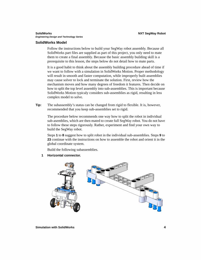
Build the following subassemblies.

1 Horizontal connector.



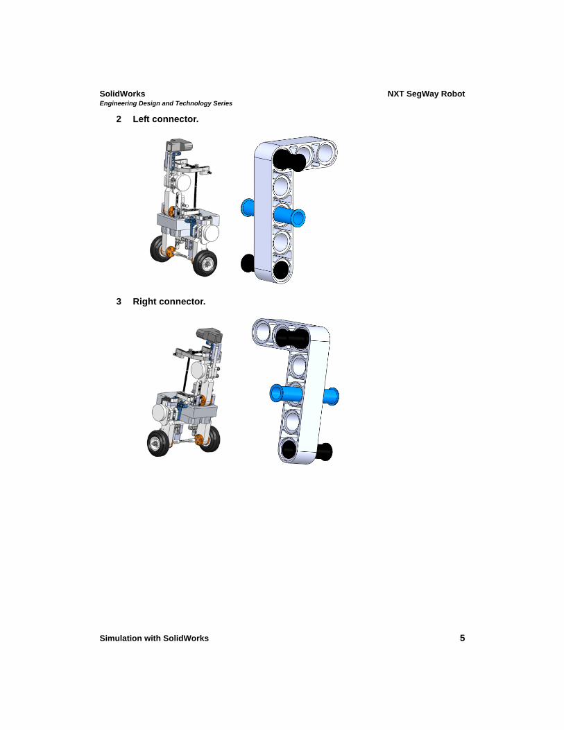
2 Left connector.

3 Right connector.



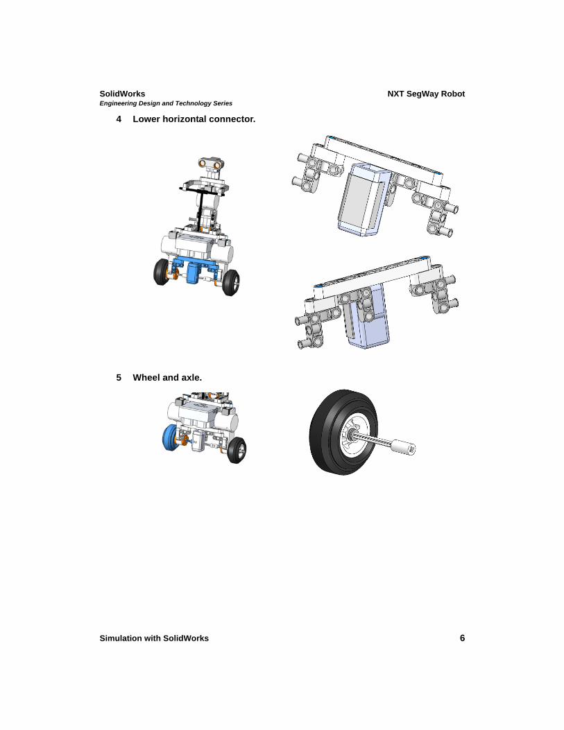
4 Lower horizontal connector.

5 Wheel and axle.



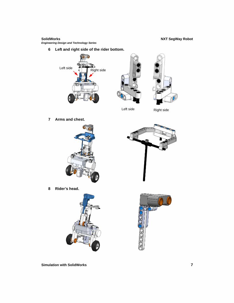
6 Left and right side of the rider bottom.

7 Arms and chest.

8 Rider’s head.

Left sideRight side

Left side Right side



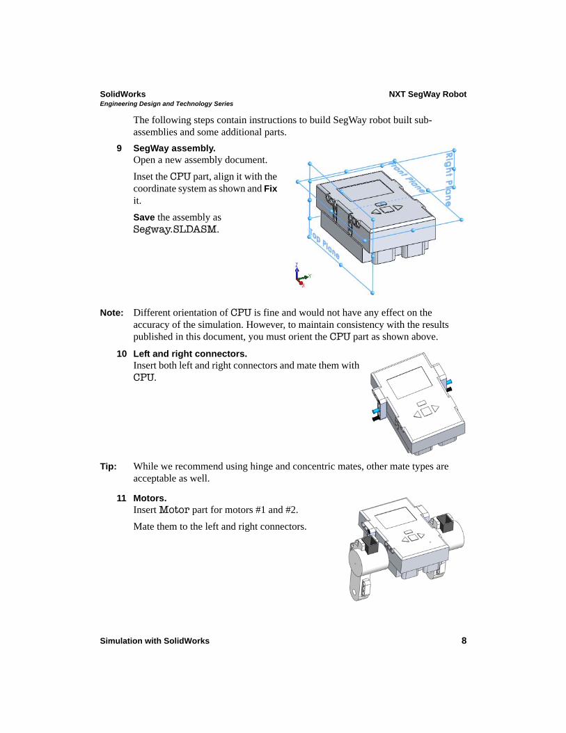
The following steps contain instructions to build SegWay robot built sub-assemblies and some additional parts.

9 SegWay assembly.Open a new assembly document.

Inset the CPU part, align it with the coordinate system as shown and Fix it.

Save the assembly as Segway.SLDASM.

Note: Different orientation of CPU is fine and would not have any effect on the accuracy of the simulation. However, to maintain consistency with the results published in this document, you must orient the CPU part as shown above.

10 Left and right connectors.Insert both left and right connectors and mate them with CPU.

Tip: While we recommend using hinge and concentric mates, other mate types are acceptable as well.

11 Motors.Insert Motor part for motors #1 and #2.

Mate them to the left and right connectors.



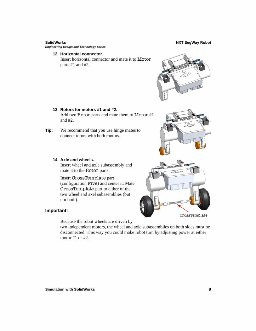
12 Horizontal connector.Insert horizontal connector and mate it to Motor parts #1 and #2.

13 Rotors for motors #1 and #2.Add two Rotor parts and mate them to Motor #1 and #2.

Tip: We recommend that you use hinge mates to connect rotors with both motors.

14 Axle and wheels.Insert wheel and axle subassembly and mate it to the Rotor parts.

Insert CrossTemplate part (configuration Five) and center it. Mate CrossTemplate part to either of the two wheel and axel subasemblies (but not both).

Important!

Because the robot wheels are driven by two independent motors, the wheel and axle subassemblies on both sides must be disconnected. This way you could make robot turn by adjusting power at either motor #1 or #2.

CrossTemplate



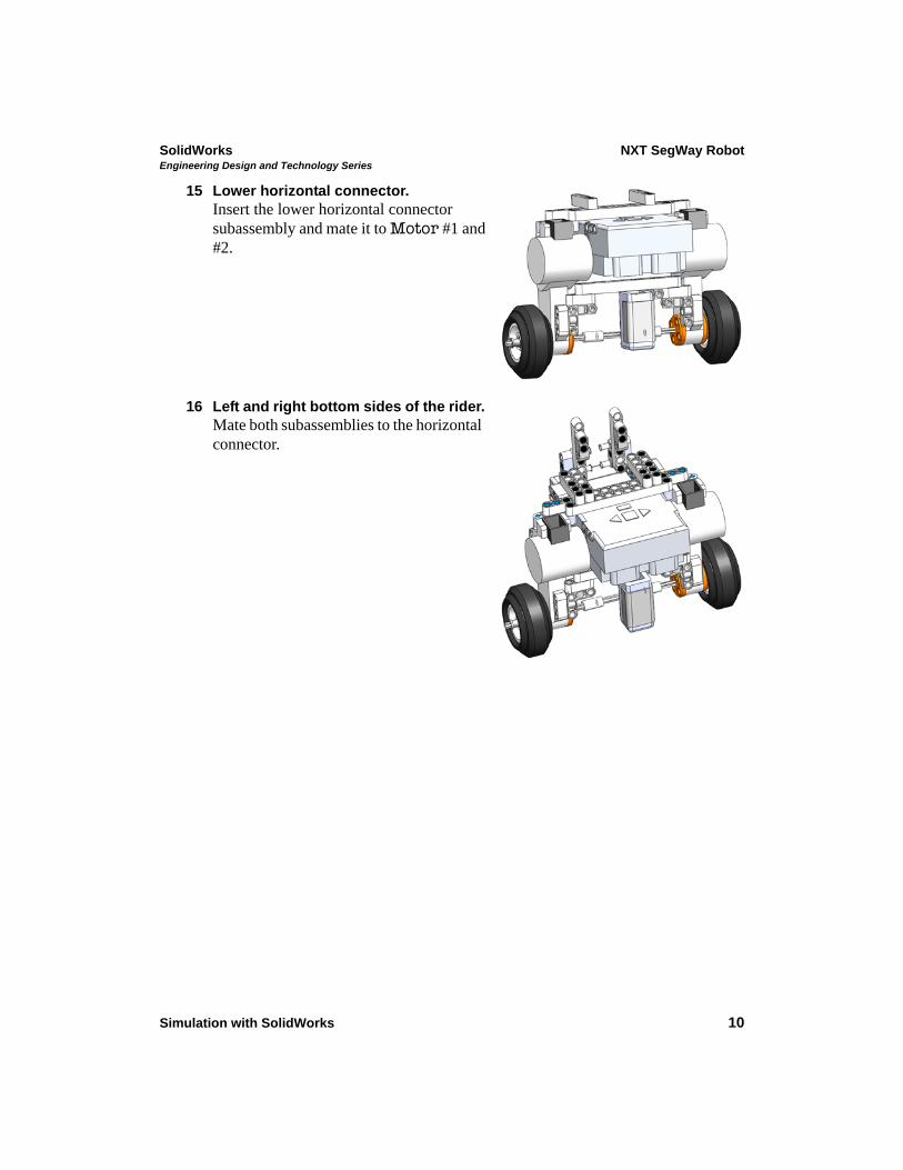
15 Lower horizontal connector.Insert the lower horizontal connector subassembly and mate it to Motor #1 and #2.

16 Left and right bottom sides of the rider.Mate both subassemblies to the horizontal connector.



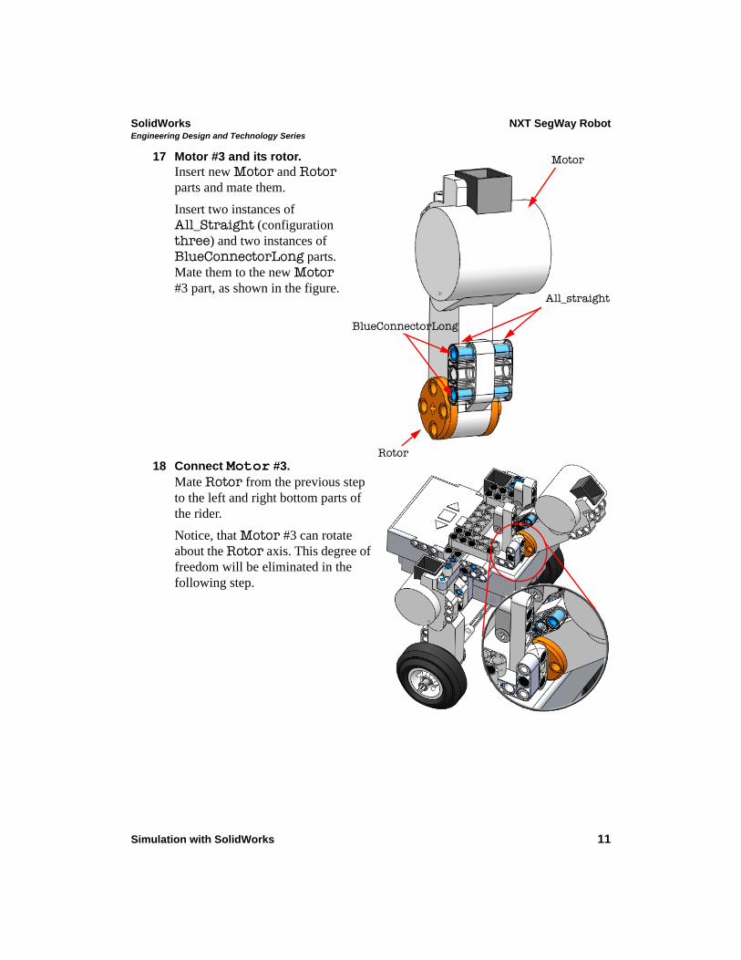
17 Motor #3 and its rotor.Insert new Motor and Rotor parts and mate them.

Insert two instances of All_Straight (configuration three) and two instances of BlueConnectorLong parts. Mate them to the new Motor #3 part, as shown in the figure.

18 Connect Motor #3.Mate Rotor from the previous step to the left and right bottom parts of the rider.

Notice, that Motor #3 can rotate about the Rotor axis. This degree of freedom will be eliminated in the following step.

All_straight

BlueConnectorLong

Rotor

Motor



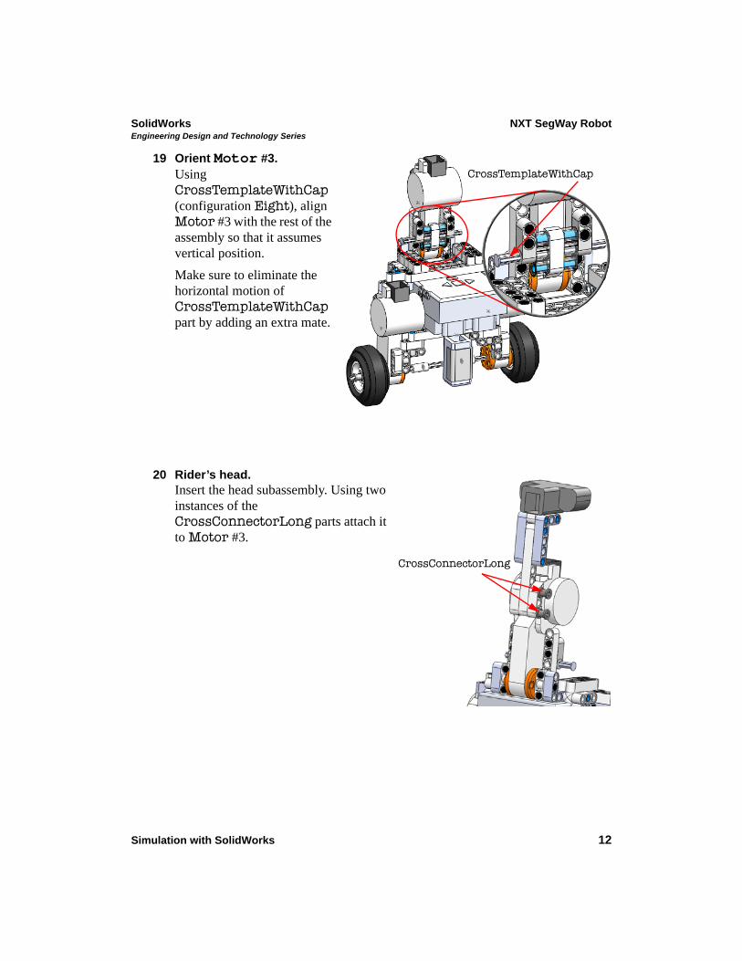
19 Orient Motor #3.Using CrossTemplateWithCap (configuration Eight), align Motor #3 with the rest of the assembly so that it assumes vertical position.

Make sure to eliminate the horizontal motion of CrossTemplateWithCappart by adding an extra mate.

20 Rider’s head.Insert the head subassembly. Using two instances of the CrossConnectorLong parts attach it to Motor #3.

CrossTemplateWithCap

CrossConnectorLong



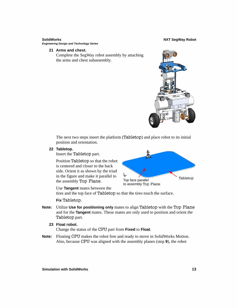
21 Arms and chest.Complete the SegWay robot assembly by attaching the arms and chest subassembly.

The next two steps insert the platform (Tabletop) and place robot to its initial position and orientation.

22 Tabletop.Insert the Tabletop part.

Position Tabletop so that the robot is centered and closer to the back side. Orient it as shown by the triad in the figure and make it parallel to the assembly Top Plane.

Use Tangent mates between the tires and the top face of Tabletop so that the tires touch the surface.

Fix Tabletop.

Note: Utilize Use for positioning only mates to align Tabletop with the Top Plane and for the Tangent mates. These mates are only used to position and orient the Tabletop part.

23 Float robot.Change the status of the CPU part from Fixed to Float.

Note: Floating CPU makes the robot free and ready to move in SolidWorks Motion. Also, because CPU was aligned with the assembly planes (step 9), the robot

TabletopTop face parallel to assembly Top Plane



assumes vertical position.

SolidWorks Motion Model

The following section will guide you through the setup of the simulation and basic control in SolidWorks Motion. As you work through this part, you will gradually improve the control algorithm so that, in its final stage, it correlates with what you observe in reality.

It is assumed that you are familiar with the basics of SolidWorks Motion software. If that is not the case, please ask your instructor to advise you on how to obtain more elementary training material to make yourself comfortable with the software.

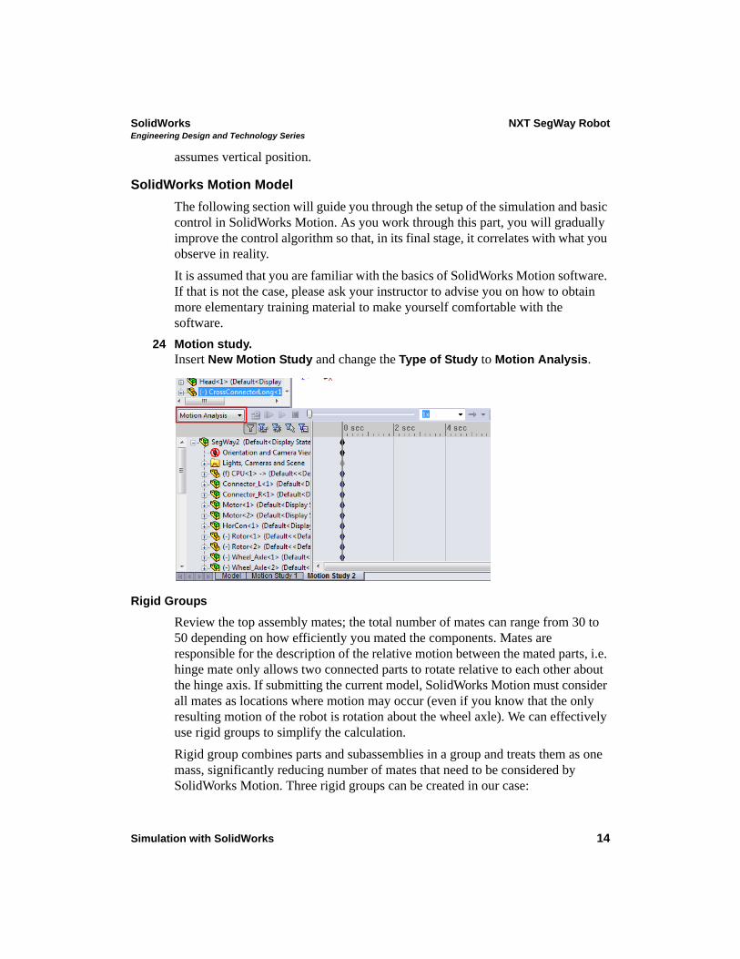
24 Motion study.Insert New Motion Study and change the Type of Study to Motion Analysis.

Rigid Groups

Review the top assembly mates; the total number of mates can range from 30 to 50 depending on how efficiently you mated the components. Mates are responsible for the description of the relative motion between the mated parts, i.e. hinge mate only allows two connected parts to rotate relative to each other about the hinge axis. If submitting the current model, SolidWorks Motion must consider all mates as locations where motion may occur (even if you know that the only resulting motion of the robot is rotation about the wheel axle). We can effectively use rigid groups to simplify the calculation.

Rigid group combines parts and subassemblies in a group and treats them as one mass, significantly reducing number of mates that need to be considered by SolidWorks Motion. Three rigid groups can be created in our case:



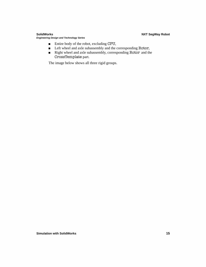
Entire body of the robot, excluding CPU, Left wheel and axle subassembly and the corresponding Rotor, Right wheel and axle subassembly, corresponding Rotor and the

CrossTemplate part.

The image below shows all three rigid groups.



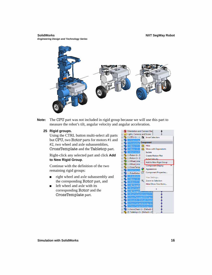
Note: The CPU part was not included in rigid group because we will use this part to measure the robot’s tilt, angular velocity and angular acceleration.

25 Rigid groups.Using the CTRL button multi-select all parts but CPU, two Rotor parts for motors #1 and #2, two wheel and axle subassemblies, CrossTemplate and the Tabletop part.

Right-click any selected part and click Add to New Rigid Group.

Continue with the definition of the two remaining rigid groups:

right wheel and axle subassembly and the correponding Rotor part, and

left wheel and axle with its corresponding Rotor and the CrossTemplate part.



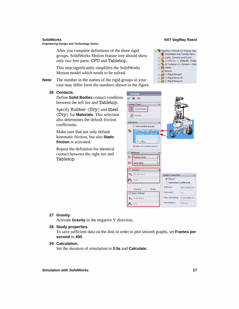
After you complete definitions of the three rigid groups, SolidWorks Motion feature tree should show only two free parts: CPU and Tabletop.

This step significantly simplifies the SolidWorks Motion model which needs to be solved.

Note: The number in the names of the rigid groups in your case may differ form the numbers shown in the figure.

26 Contacts.Define Solid Bodies contact condition between the left tire and Tabletop.

Specify Rubber (Dry) and Steel (Dry) for Materials. This selection also determines the default friction coefficients.

Make sure that not only default kinematic friction, but also Static friction is activated.

Repeat the definition for identical contact between the right tire and Tabletop.

27 Gravity.Activate Gravity in the negative Y direction.

28 Study properties.To save sufficient data on the disk in order to plot smooth graphs, set Frames per second to 400.

29 Calculation.Set the duration of simulation to 0.5s and Calculate.



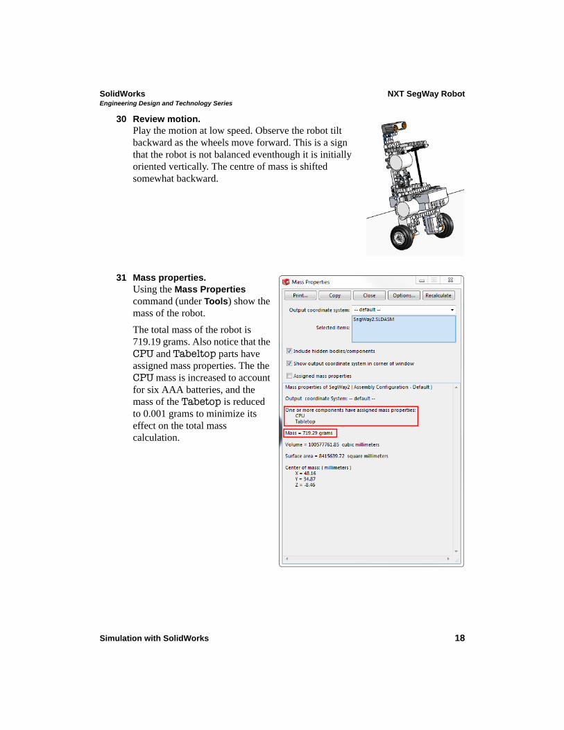
30 Review motion.Play the motion at low speed. Observe the robot tilt backward as the wheels move forward. This is a sign that the robot is not balanced eventhough it is initially oriented vertically. The centre of mass is shifted somewhat backward.

31 Mass properties.Using the Mass Properties command (under Tools) show the mass of the robot.

The total mass of the robot is 719.19 grams. Also notice that the CPU and Tabeltop parts have assigned mass properties. The the CPU mass is increased to account for six AAA batteries, and the mass of the Tabetop is reduced to 0.001 grams to minimize its effect on the total mass calculation.



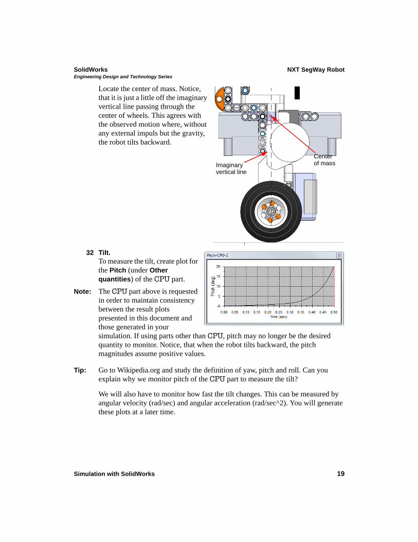
Locate the center of mass. Notice, that it is just a little off the imaginary vertical line passing through the center of wheels. This agrees with the observed motion where, without any external impuls but the gravity, the robot tilts backward.

32 Tilt.To measure the tilt, create plot for the Pitch (under Other quantities) of the CPU part.

Note: The CPU part above is requested in order to maintain consistency between the result plots presented in this document and those generated in your simulation. If using parts other than CPU, pitch may no longer be the desired quantity to monitor. Notice, that when the robot tilts backward, the pitch magnitudes assume positive values.

Tip: Go to Wikipedia.org and study the definition of yaw, pitch and roll. Can you explain why we monitor pitch of the CPU part to measure the tilt?

We will also have to monitor how fast the tilt changes. This can be measured by angular velocity (rad/sec) and angular acceleration (rad/sec^2). You will generate these plots at a later time.

Imaginaryvertical line

Centerof mass



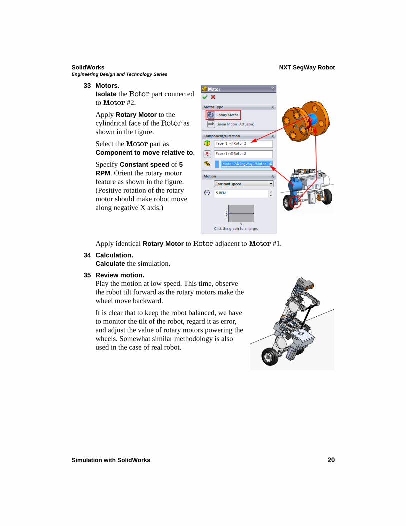
33 Motors.Isolate the Rotor part connected to Motor #2.

Apply Rotary Motor to the cylindrical face of the Rotor as shown in the figure.

Select the Motor part as Component to move relative to.

Specify Constant speed of 5 RPM. Orient the rotary motor feature as shown in the figure. (Positive rotation of the rotary motor should make robot move along negative X axis.)

Apply identical Rotary Motor to Rotor adjacent to Motor #1.

34 Calculation.Calculate the simulation.

35 Review motion.Play the motion at low speed. This time, observe the robot tilt forward as the rotary motors make the wheel move backward.

It is clear that to keep the robot balanced, we have to monitor the tilt of the robot, regard it as error, and adjust the value of rotary motors powering the wheels. Somewhat similar methodology is also used in the case of real robot.



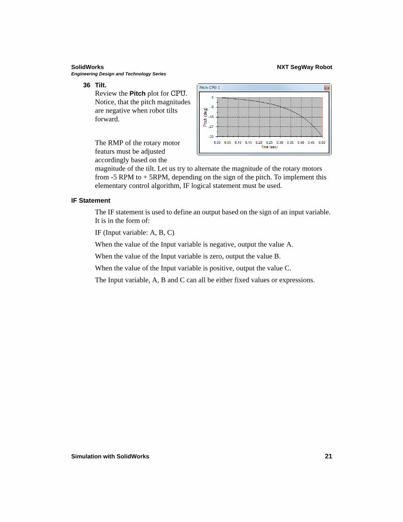
36 Tilt.Review the Pitch plot for CPU. Notice, that the pitch magnitudes are negative when robot tilts forward.

The RMP of the rotary motor featurs must be adjusted accordingly based on the magnitude of the tilt. Let us try to alternate the magnitude of the rotary motors from -5 RPM to + 5RPM, depending on the sign of the pitch. To implement this elementary control algorithm, IF logical statement must be used.

IF Statement

The IF statement is used to define an output based on the sign of an input variable. It is in the form of:

IF (Input variable: A, B, C)

When the value of the Input variable is negative, output the value A.

When the value of the Input variable is zero, output the value B.

When the value of the Input variable is positive, output the value C.

The Input variable, A, B and C can all be either fixed values or expressions.



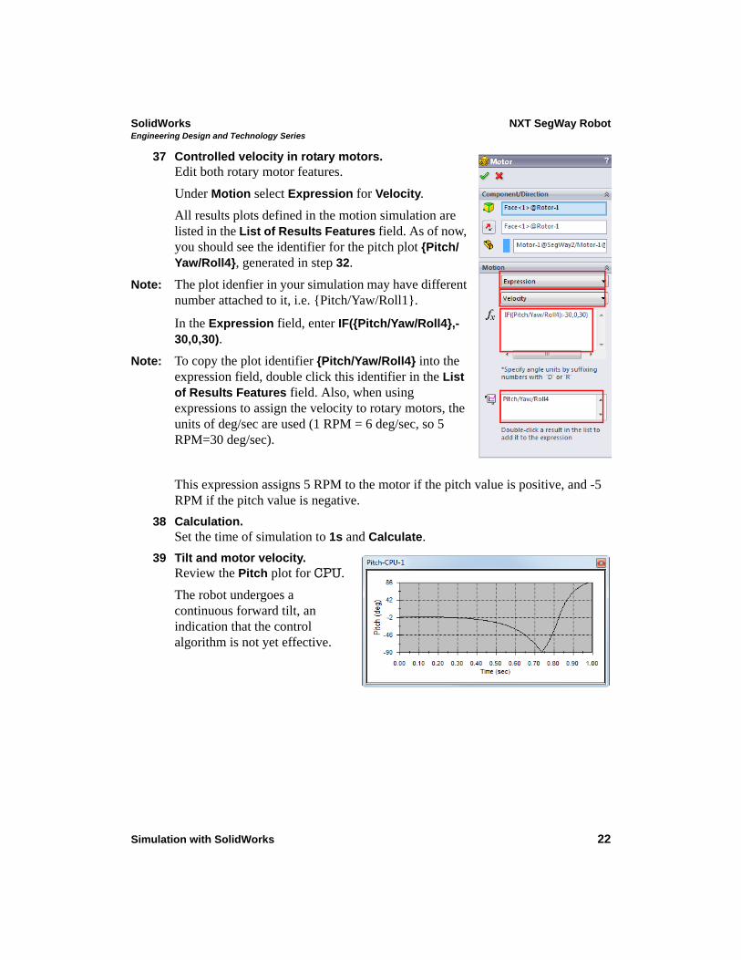
37 Controlled velocity in rotary motors.Edit both rotary motor features.

Under Motion select Expression for Velocity.

All results plots defined in the motion simulation are listed in the List of Results Features field. As of now, you should see the identifier for the pitch plot {Pitch/Yaw/Roll4}, generated in step 32.

Note: The plot idenfier in your simulation may have different number attached to it, i.e. {Pitch/Yaw/Roll1}.

In the Expression field, enter IF({Pitch/Yaw/Roll4},-30,0,30).

Note: To copy the plot identifier {Pitch/Yaw/Roll4} into the expression field, double click this identifier in the List of Results Features field. Also, when using expressions to assign the velocity to rotary motors, the units of deg/sec are used (1 RPM = 6 deg/sec, so 5 RPM=30 deg/sec).

This expression assigns 5 RPM to the motor if the pitch value is positive, and -5 RPM if the pitch value is negative.

38 Calculation.Set the time of simulation to 1s and Calculate.

39 Tilt and motor velocity.Review the Pitch plot for CPU.

The robot undergoes a continuous forward tilt, an indication that the control algorithm is not yet effective.



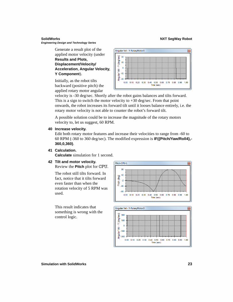
Generate a result plot of the applied motor velocity (under Results and Plots, Displacement/Velocity/Acceleration, Angular Velocity, Y Component).

Initially, as the robot tilts backward (positive pitch) the applied rotary motor angular velocity is -30 deg/sec. Shortly after the robot gains balances and tilts forward. This is a sign to switch the motor velocity to +30 deg/sec. From that point onwards, the robot increases its forward tilt until it looses balance entirely, i.e. the rotary motor velocity is not able to counter the robot’s forward tilt.

A possible solution could be to increase the magnitude of the rotary motors velocity to, let us suggest, 60 RPM.

40 Increase velocity.Edit both rotary motor features and increase their velocities to range from -60 to 60 RPM (-360 to 360 deg/sec). The modified expression is IF({Pitch/Yaw/Roll4},-360,0,360).

41 Calculation.Calculate simulation for 1 second.

42 Tilt and motor velocity.Review the Pitch plot for CPU.

The robot still tilts forward. In fact, notice that it tilts forward even faster than when the rotation velocity of 5 RPM was used.

This result indicates that something is wrong with the control logic.



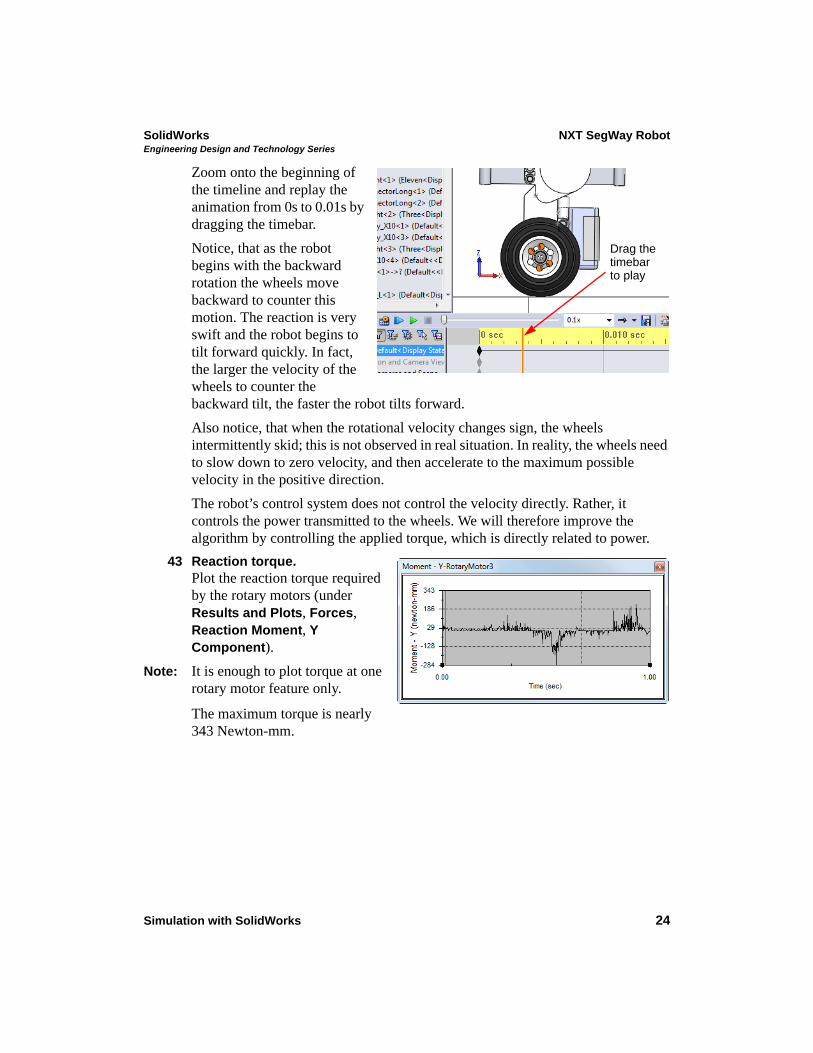
Zoom onto the beginning of the timeline and replay the animation from 0s to 0.01s by dragging the timebar.

Notice, that as the robot begins with the backward rotation the wheels move backward to counter this motion. The reaction is very swift and the robot begins to tilt forward quickly. In fact, the larger the velocity of the wheels to counter the backward tilt, the faster the robot tilts forward.

Also notice, that when the rotational velocity changes sign, the wheels intermittently skid; this is not observed in real situation. In reality, the wheels need to slow down to zero velocity, and then accelerate to the maximum possible velocity in the positive direction.

The robot’s control system does not control the velocity directly. Rather, it controls the power transmitted to the wheels. We will therefore improve the algorithm by controlling the applied torque, which is directly related to power.

43 Reaction torque.Plot the reaction torque required by the rotary motors (under Results and Plots, Forces, Reaction Moment, Y Component).

Note: It is enough to plot torque at one rotary motor feature only.

The maximum torque is nearly 343 Newton-mm.

Drag thetimebarto play



Maximum torque

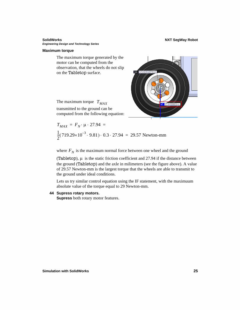
The maximum torque generated by the motor can be computed from the observation, that the wheels do not slip on the Tabletop surface.

The maximum torque

transmitted to the ground can be computed from the following equation:

where is the maximum normal force between one wheel and the ground

(Tabletop), is the static friction coefficient and 27.94 if the distance between the ground (Tabletop) and the axle in milimeters (see the figure above). A value of 29.57 Newton-mm is the largest torque that the wheels are able to transmit to the ground under ideal conditions.

Lets us try similar control equation using the IF statement, with the maximuum absolute value of the torque equal to 29 Newton-mm.

44 Supress rotary motors.Supress both rotary motor features.

TMAX

TMAX FN 27.94

12--- 719.29

3–10 9.81 0.3 27.94 29.57 Newton-mm

= =

=

FN



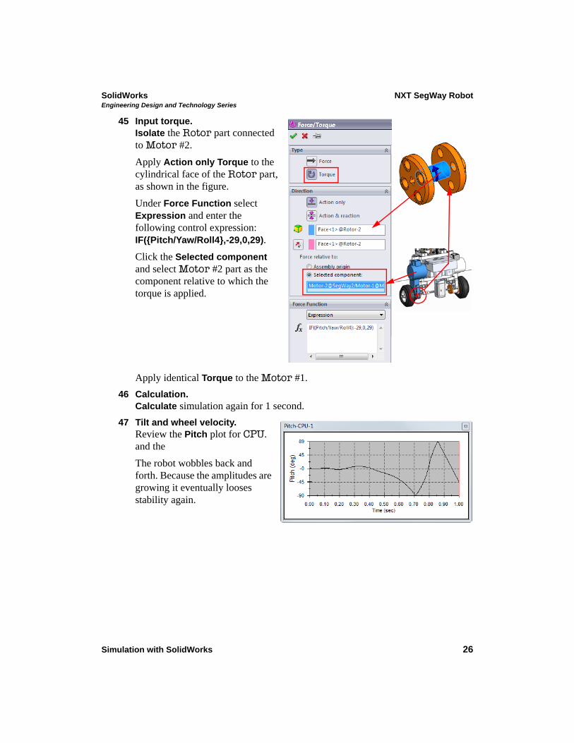
45 Input torque.Isolate the Rotor part connected to Motor #2.

Apply Action only Torque to the cylindrical face of the Rotor part, as shown in the figure.

Under Force Function select Expression and enter the following control expression: IF({Pitch/Yaw/Roll4},-29,0,29).

Click the Selected component and select Motor #2 part as the component relative to which the torque is applied.

Apply identical Torque to the Motor #1.

46 Calculation.Calculate simulation again for 1 second.

47 Tilt and wheel velocity.Review the Pitch plot for CPU. and the

The robot wobbles back and forth. Because the amplitudes are growing it eventually looses stability again.



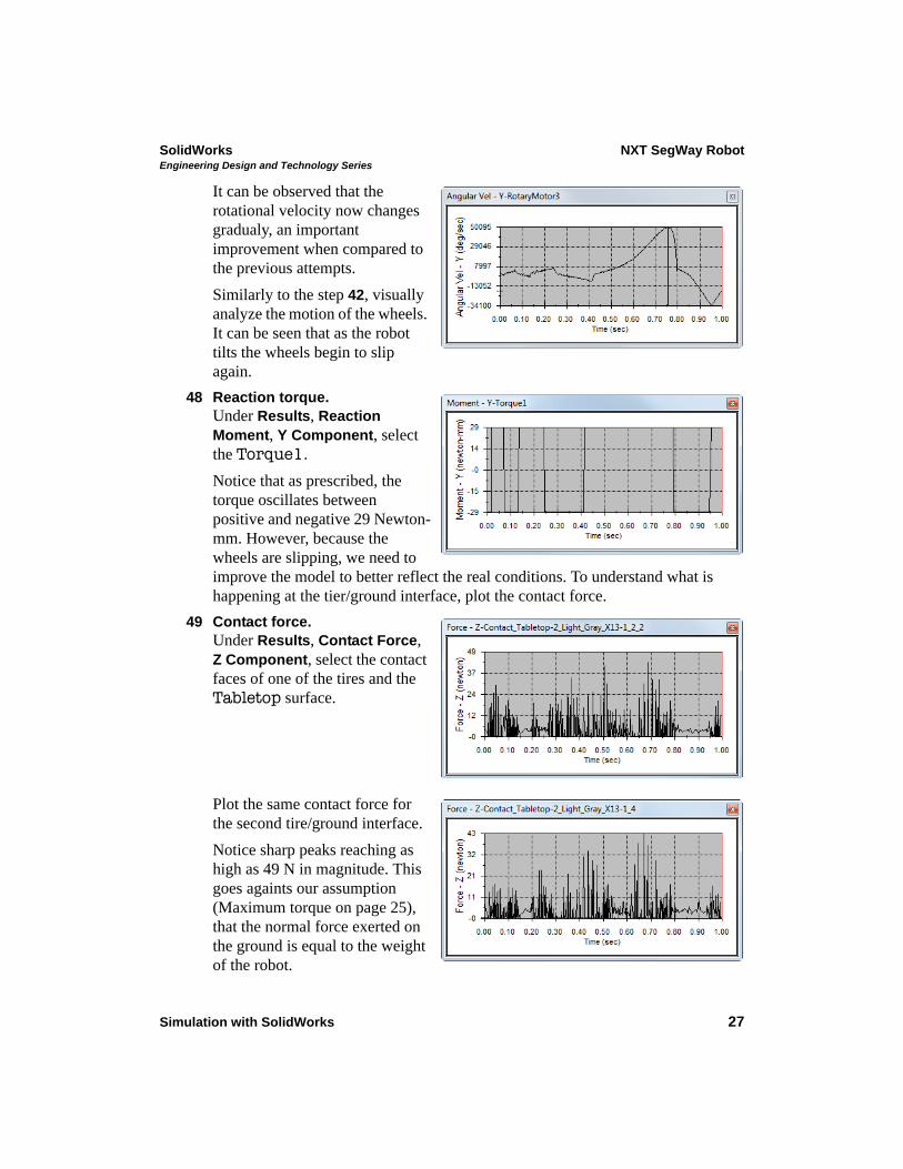
It can be observed that the rotational velocity now changes gradualy, an important improvement when compared to the previous attempts.

Similarly to the step 42, visually analyze the motion of the wheels. It can be seen that as the robot tilts the wheels begin to slip again.

48 Reaction torque.Under Results, Reaction Moment, Y Component, select the Torque1.

Notice that as prescribed, the torque oscillates between positive and negative 29 Newton-mm. However, because the wheels are slipping, we need to improve the model to better reflect the real conditions. To understand what is happening at the tier/ground interface, plot the contact force.

49 Contact force.Under Results, Contact Force, Z Component, select the contact faces of one of the tires and the Tabletop surface.

Plot the same contact force for the second tire/ground interface.

Notice sharp peaks reaching as high as 49 N in magnitude. This goes againts our assumption (Maximum torque on page 25), that the normal force exerted on the ground is equal to the weight of the robot.



The sharp peaks signal that the robot’s travel is uneven exhibitting numerous intermittent jumps. Nothing similar is observed in the real situation. The reason for this behavior is innacurate characterization of contact between the tires and the ground, i.e. the contact stiffness is too high.

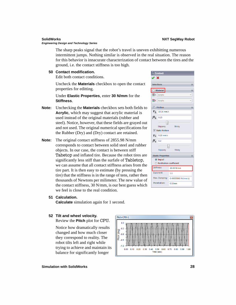
50 Contact modification.Edit both contact conditions.

Uncheck the Materials checkbox to open the contact properties for editting.

Under Elastic Properties, enter 30 N/mm for the Stiffness.

Note: Unchecking the Materials checkbox sets both fields to Acrylic, which may suggest that acrylic material is used instead of the original materials (rubber and steel). Notice, however, that these fields are grayed out and not used. The original numerical specifications for the Rubber (Dry) and (Dry) contact are retained.

Note: The original contact stiffness of 2855.98 N/mm corresponds to contact between solid steel and rubber objects. In our case, the contact is between stiff Tabetop and inflated tire. Because the robot tires are significantly less stiff than the surfafe of Tabletop, we can assume that all contact stiffness arises from the tire part. It is then easy to estimate (by pressing the tire) that the stiffness is in the range of tens, rather then thousands of Newtons per milimeter. The new value of the contact stiffness, 30 N/mm, is our best guess which we feel is close to the real condition.


52 Tilt and wheel velocity.Review the Pitch plot for CPU.

Notice how dramatically results changed and how much closer they correspond to reality. The robot tilts left and right while trying to achieve and maintain its balance for significantly longer



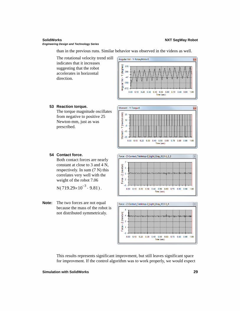
than in the previous runs. Similar behavior was observed in the videos as well.

The rotational velocity trend still indicates that it increases suggesting that the robot accelerates in horizontal direction.

53 Reaction torque.The torque magnitude oscillates from negative to positive 25 Newton-mm, just as was prescribed.

54 Contact force.Both contact forces are nearly constant at close to 3 and 4 N, respectively. In sum (7 N) this correlates very well with the weight of the robot 7.06

N .

Note: The two forces are not equal because the mass of the robot is not distributed symmetricaly.

This results represents significant improvment, but still leaves significant space for improvment. If the control algorithm was to work properly, we would expect

719.293–10 9.81



the rotational velocity (as well as the tilt) to attenuate. Because it appears that we have exhausted the capability of the current elementary control algorithm (single IF logical statement with constant input torque) more advanced algorithm is necessary.

PID Control

PID control is one of numerous control algorithms used in the industry and robotics. The PID stands for Proportional, Integral and Derivative control algorithm. To demonstrate this algorithm, consider the following.

Our goal is to achieve and maintain the robot’s balance. The first approach was to eliminate tilt by means of applying external torque at the wheels. This, thus far, has proven not effective.

Consider the result plot of the tilt generated in step 52. The robot reaches zero tilt configuration in each cycle, but fails to eliminate it. At each zero tilt configuration the robot reaches significant rotational velocity (pendulum swing) increasing the tilt on the opposite side. In fact, such behavior can be self-propelling and stable balance may not be found. In order to stabilize the robot at zero tilt configuration we must also require that its rotational velocity is zero (to stop it from swinging past the stable configuration). This requirement may be enough, or we maygo even further and require that not only rotational velocity but also rotational acceleration be zero.

The case where tilt and rotational velocity are controlled is referred to as PI algorithm (Proportional and Integral). The most advanced case when all three quantities are controlled is known as PID (Proportional, Integral and Derivative).

In the next section of this lesson we will implement PID controller. To apply PID control, let us define the rotational velocity of the CPU part as error. Then, since the angular displacement (or tilt) is equal to the integral of the angular velocity, the tilt will represent the I-portion (or the integral portion) of the PID controller. Finally, because the angular acceleration is equal to the derivate of the angular velocity, the angular acceleration will represent the D-portion (or the derivative portion) of the PID controller. With the above definition of error, the control equation for the PID controller will be in the following form:

where is the applied torque, is the tilt, is the angular velocity of CPU, is

the angular acceleration of CPU and multipliers are the proportionality

constants, or gain coefficients. These constants represent our input for the control algorithm.

T k1 k2 v k3 a++=

T v a

k1 2 3



To implement PID control, we first have to plot the angular velocity and the angular acceleration of CPU (angular displacement, or tilt, was already plotted a few times in the previous steps).

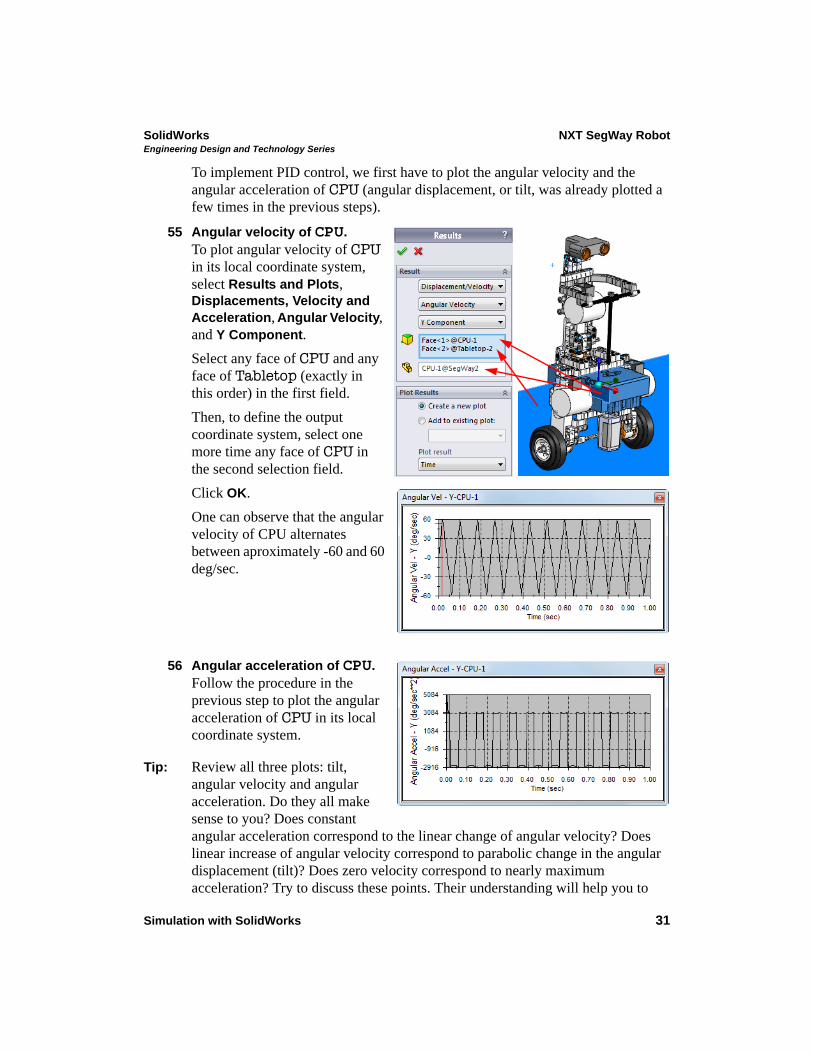
55 Angular velocity of CPU.To plot angular velocity of CPU in its local coordinate system, select Results and Plots, Displacements, Velocity and Acceleration, Angular Velocity, and Y Component.

Select any face of CPU and any face of Tabletop (exactly in this order) in the first field.

Then, to define the output coordinate system, select one more time any face of CPU in the second selection field.

Click OK.

One can observe that the angular velocity of CPU alternates between aproximately -60 and 60 deg/sec.

56 Angular acceleration of CPU.Follow the procedure in the previous step to plot the angular acceleration of CPU in its local coordinate system.

Tip: Review all three plots: tilt, angular velocity and angular acceleration. Do they all make sense to you? Does constant angular acceleration correspond to the linear change of angular velocity? Does linear increase of angular velocity correspond to parabolic change in the angular displacement (tilt)? Does zero velocity correspond to nearly maximum acceleration? Try to discuss these points. Their understanding will help you to



understand why it is beneficial to control all three quantities (PID control) rather then just the tilt.

PID Control of Segway robot

As was explained in the previous paragraphs, the PID control requires continuous adjustment of the input quantity (Torque) as a function of the error quantity (angular velocity), and its integral and derivative (tilt and angular acceleration). The control equation was shown in the PID Control on page 30. Now, consider the directions of the tilt, angular velocity, angular acceleration and the input torque to conclude that in order to balance the robot, the following holds:

When tilt of CPU is positive, the input torque must be positive. When angular velocity of CPU is positive, the input torque must be negative. When angular acceleration of CPU is positive, the input torque must be

negative.

With this in mind, the PID control equation will look as follows:

We will now edit the expression for the input torque to reflect the PID control equation above.

T k1 k2 v k3 a––=



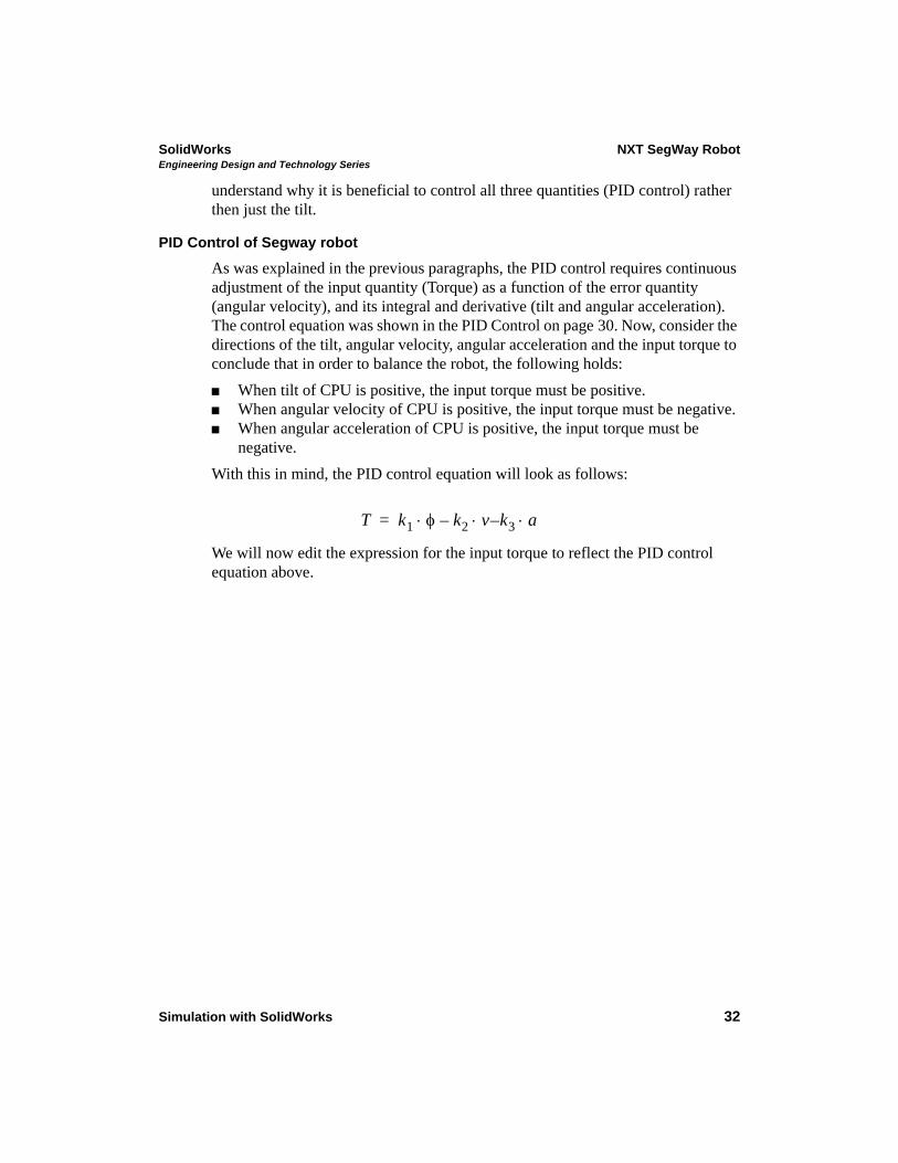
57 Edit input torque.Edit either of the two torque features.

Modify their expression to the following: 1*{Pitch/Yaw/Roll4}-1*{Angular Velocity6}-1*{Angular Acceleration1}.

Note: The plot idenfiers in your simulation may again have different numbers attached to them, i.e. {Angular Velocity1} or {Angular Acceleration3}.


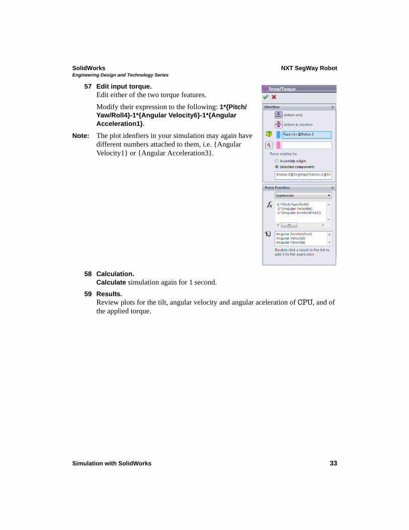
59 Results.Review plots for the tilt, angular velocity and angular aceleration of CPU, and of the applied torque.



Reviewing the above plots and the animation of the robot motion suggests that the control is working pretty good. The problem is that it does not correspond too closely to the real observation. The robot does not tilt too much and the applied torque is very small (it is apparent from the videos that maximum torque is applied occasionally). We can say that the controller is tuned too stiff, not fitting the current situation well.

The three gain coefficients have thus far all been kept at a default value of 1. In order for the control to work effectively and correspond to the observations, the system needs to be tuned.

When the controller is tuned, we expect the torque to occasionaly reach the maximum magnitude of 29 N.

The next two sections will set the limit of the applied torque to 29 N and tune the controller by adjusting the gain coeffficients.

Maximum torque limit

The torque magnitude must be limited to the maximum which can be transmitted to the ground without wheels slipping on the surface of Tabletop (29.57 Newton-mm, Maximum torque on page 25). We can make use of the IF statement (page 21) and construct the following logical statement.

IF(PositiveLimit-Torque:PositiveLimit,PositiveLimit,(IF(NegativeLimit-Torque:Torque,NegativeLimit,NegativeLimit)))

In the statement above, Torque is the expression for the input torque from step 57,

Tilt Rotational velocity

Rotational acceleration Applied torque



PositiveLimit=29 Newton-mm and NegativeLimit=-29 Newton-mm. Take a moment and try to understand the above statement and how it works.

Combining the above complex IF statement with the expression for the torque (step 57), and its limiting values (-29 and 29 Newton-mm) results in the following lengthy statement:

IF(29-(10*{Pitch/Yaw/Roll4}-0.1*{Angular Velocity6}-0.01*{Angular Acceleration1}):29,29,(IF(-29-(10*{Pitch/Yaw/Roll4}-0.1*{Angular Velocity6}-0.01*{Angular Acceleration1}):(10*{Pitch/Yaw/Roll4}-0.1*{Angular Velocity6}-0.01*{Angular Acceleration1}),-29,-29)))

The above expression uses the correct control expression for the input torque (step 57) and limits its absolute magnitude to 29 Netwon-mm. The next section elaborates somewhat on tuning the control expression.

Tunning PID Control

Tuning the digital PID control mechanism requires adjustment of the three gain constants until users are satisfied with the outcome. As you can expect, tuning three contstants without any educated methodology can be a time consuming task. In this lesson, our goal is to tune the constants so that the robot gains balance and its behavior corresponds to the videos. The following coefficients will be used:

60 Edit input torque.Modify the gain coefficients in the expression for both input torques as follows: IF(29-(10*{Pitch/Yaw/Roll4}-0.1*{Angular Velocity6}-0.01*{Angular Acceleration1}):29,29,(IF(-29-(10*{Pitch/Yaw/Roll4}-0.1*{Angular Velocity6}-0.01*{Angular Acceleration1}):(10*{Pitch/Yaw/Roll4}-0.1*{Angular Velocity6}-0.01*{Angular Acceleration1}),-29,-29))).

61 Calculation.Calculate simulation again for 2s.

Note: The time of calculation is increased in order to give control equation enough time to reach balance.

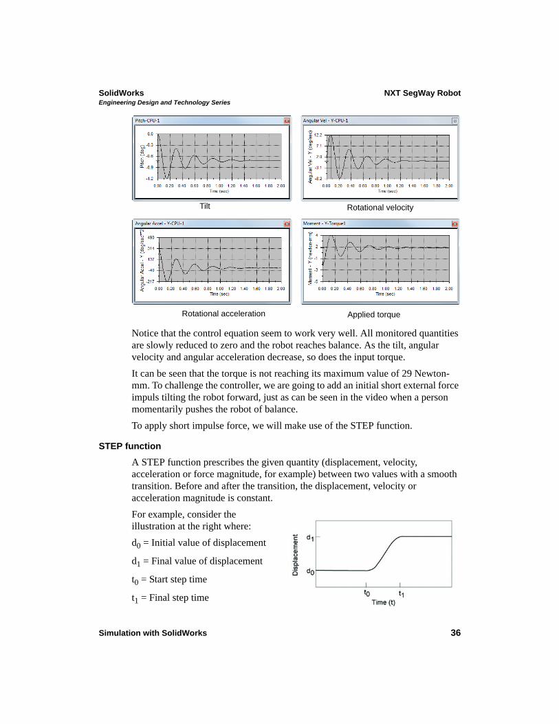
62 Results.Review the plots for the tilt, angular velocity and angular aceleration of CPU, and of the applied torque.

k1 10=

k2 0.1=

k3 0.01=



Notice that the control equation seem to work very well. All monitored quantities are slowly reduced to zero and the robot reaches balance. As the tilt, angular velocity and angular acceleration decrease, so does the input torque.

It can be seen that the torque is not reaching its maximum value of 29 Newton-mm. To challenge the controller, we are going to add an initial short external force impuls tilting the robot forward, just as can be seen in the video when a person momentarily pushes the robot of balance.

To apply short impulse force, we will make use of the STEP function.

STEP function

A STEP function prescribes the given quantity (displacement, velocity, acceleration or force magnitude, for example) between two values with a smooth transition. Before and after the transition, the displacement, velocity or acceleration magnitude is constant.

For example, consider the illustration at the right where:

d0 = Initial value of displacement

d1 = Final value of displacement

t0 = Start step time

t1 = Final step time





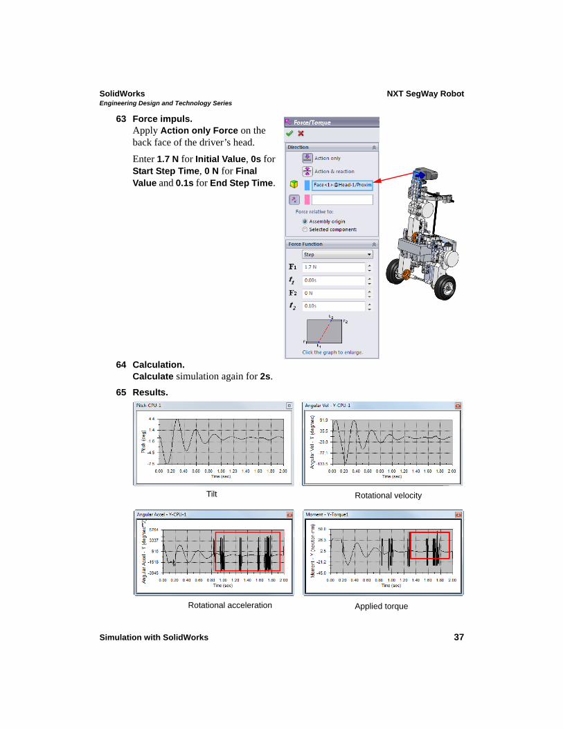
63 Force impuls.Apply Action only Force on the back face of the driver’s head.

Enter 1.7 N for Initial Value, 0s for Start Step Time, 0 N for Final Value and 0.1s for End Step Time.


65 Results.





We can observe, that the tilt of the CPU part is controlled well, but some disturbances are seen in the plot of the rotational acceleration and the input torque (input torque is dependent on the acceleration).

In some situations, calculation of accelerations is not as accurate as calculation of the displacements and velocities. To improve the calculation of accelerations, an advanced integrator type can be use.

66 Study Properties.In the Motion Study Properties, click the Advanced Options button and select SI2_GSTIFF integrator.

Note: The detailed description of the integrators goes beyond the scope of this lesson.


Note: The computation with SI2_GSTIFF may take significantly longer to complete.

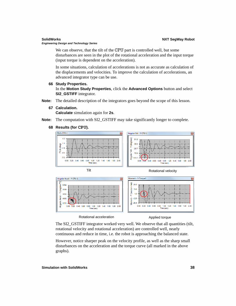
68 Results (for CPU).

The SI2_GSTIFF integrator worked very well. We observe that all quantities (tilt, rotational velocity and rotational acceleration) are controlled well, nearly continuous and reduce in time, i.e. the robot is approaching the balanced state.

However, notice sharper peak on the velocity profile, as well as the sharp small disturbances on the acceleration and the torque curve (all marked in the above graphs).





It may not be immediately apparent what happaned, so we will have to help ourself with by generating an additional result plot for the angular velocity of one of the wheels.

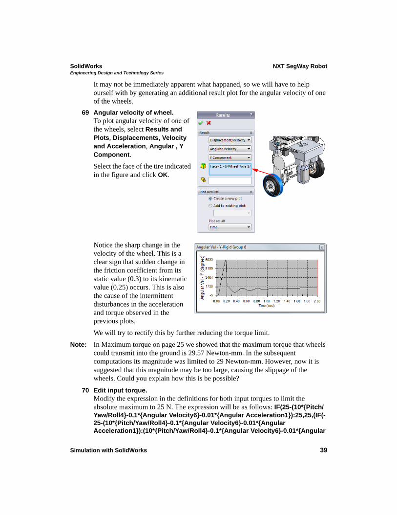
69 Angular velocity of wheel.To plot angular velocity of one of the wheels, select Results and Plots, Displacements, Velocity and Acceleration, Angular , Y Component.

Select the face of the tire indicated in the figure and click OK.

Notice the sharp change in the velocity of the wheel. This is a clear sign that sudden change in the friction coefficient from its static value (0.3) to its kinematic value (0.25) occurs. This is also the cause of the intermittent disturbances in the acceleration and torque observed in the previous plots.

We will try to rectify this by further reducing the torque limit.

Note: In Maximum torque on page 25 we showed that the maximum torque that wheels could transmit into the ground is 29.57 Newton-mm. In the subsequent computations its magnitude was limited to 29 Newton-mm. However, now it is suggested that this magnitude may be too large, causing the slippage of the wheels. Could you explain how this is be possible?

70 Edit input torque.Modify the expression in the definitions for both input torques to limit the absolute maximum to 25 N. The expression will be as follows: IF(25-(10*{Pitch/Yaw/Roll4}-0.1*{Angular Velocity6}-0.01*{Angular Acceleration1}):25,25,(IF(-25-(10*{Pitch/Yaw/Roll4}-0.1*{Angular Velocity6}-0.01*{Angular Acceleration1}):(10*{Pitch/Yaw/Roll4}-0.1*{Angular Velocity6}-0.01*{Angular



Acceleration1}),-25,-25))).


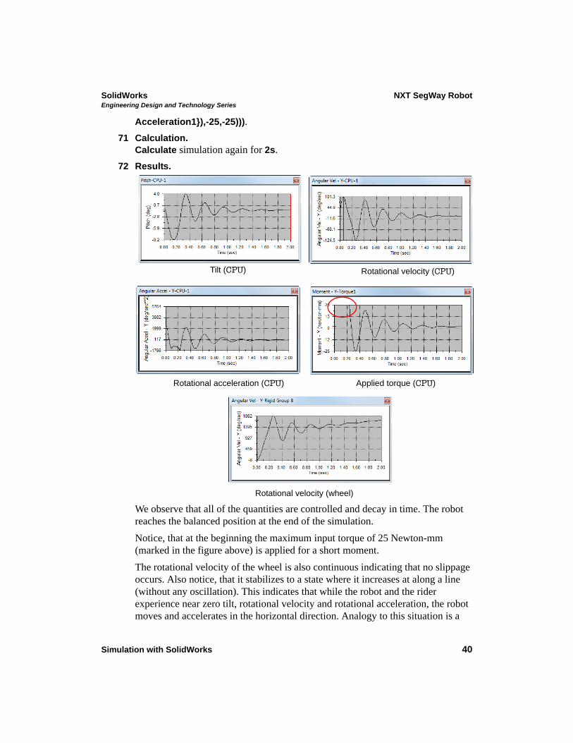
72 Results.

We observe that all of the quantities are controlled and decay in time. The robot reaches the balanced position at the end of the simulation.

Notice, that at the beginning the maximum input torque of 25 Newton-mm (marked in the figure above) is applied for a short moment.

The rotational velocity of the wheel is also continuous indicating that no slippage occurs. Also notice, that it stabilizes to a state where it increases at along a line (without any oscillation). This indicates that while the robot and the rider experience near zero tilt, rotational velocity and rotational acceleration, the robot moves and accelerates in the horizontal direction. Analogy to this situation is a

Tilt (CPU) Rotational velocity (CPU)

Rotational acceleration (CPU) Applied torque (CPU)

Rotational velocity (wheel)



rider on real SegWay transporter at a stable position, leaning slightly forward and accelerating. Further control to slow and speed up the horizontal motion of the robot would require more advanced algorithm.

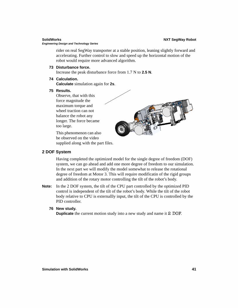
73 Disturbance force.Increase the peak disturbance force from 1.7 N to 2.5 N.


75 Results.Observe, that with this force magnitude the maximum torque and wheel traction can not balance the robot any longer. The force became too large.

This phenomenon can also be observed on the video supplied along with the part files.

2 DOF System

Having completed the optimized model for the single degree of freedom (DOF) system, we can go ahead and add one more degree of freedom to our simulation. In the next part we will modify the model somewhat to release the rotational degree of freedom at Motor 3. This will require modificatin of the rigid groups and addition of the rotary motor controlling the tilt of the robot’s body.

Note: In the 2 DOF system, the tilt of the CPU part controlled by the optimized PID control is independent of the tilt of the robot’s body. While the tilt of the robot body relative to CPU is externallly input, the tilt of the CPU is controlled by the PID controller.

76 New study.Duplicate the current motion study into a new study and name it 2 DOF.



77 Main rigid group.Delete the large rigid group which contained majority of the robot’s parts and subasemblies.

Note: As you delete this rigid groups, all parts and subassemblies will become visible in the SolidWorks Motion feature tree. In the next step, they will be re-grouped into two new rigid groups.

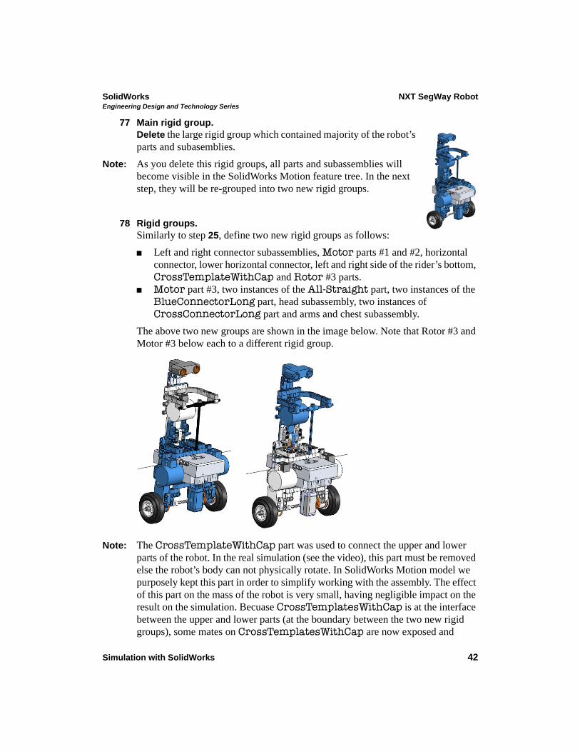
78 Rigid groups.Similarly to step 25, define two new rigid groups as follows:

Left and right connector subassemblies, Motor parts #1 and #2, horizontal connector, lower horizontal connector, left and right side of the rider’s bottom, CrossTemplateWithCap and Rotor #3 parts.

Motor part #3, two instances of the All-Straight part, two instances of the BlueConnectorLong part, head subassembly, two instances of CrossConnectorLong part and arms and chest subassembly.

The above two new groups are shown in the image below. Note that Rotor #3 and Motor #3 below each to a different rigid group.

Note: The CrossTemplateWithCap part was used to connect the upper and lower parts of the robot. In the real simulation (see the video), this part must be removed else the robot’s body can not physically rotate. In SolidWorks Motion model we purposely kept this part in order to simplify working with the assembly. The effect of this part on the mass of the robot is very small, having negligible impact on the result on the simulation. Becuase CrossTemplatesWithCap is at the interface between the upper and lower parts (at the boundary between the two new rigid groups), some mates on CrossTemplatesWithCap are now exposed and



included in the simulation. For the simulation to work, the mates connecting the upper part and the CrossTemplateWithCap part must be supressed.

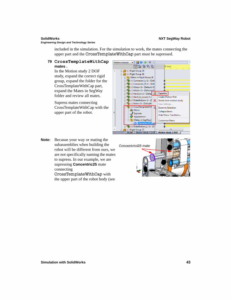
79 CrossTemplateWithCap mates .In the Motion study 2 DOF study, expand the correct rigid group, expand the folder for the CrossTemplateWithCap part, expand the Mates in SegWay folder and review all mates.

Supress mates connecting CrossTemplateWithCap with the upper part of the robot.

Note: Becasue your way or mating the subassemblies when building the robot will be different from ours, we are not specifically naming the mates to supress. In our example, we are supressing Concentric25 mate connecting CrossTemplateWithCap with the upper part of the robot body (see

Concentric25 mate



the figure).

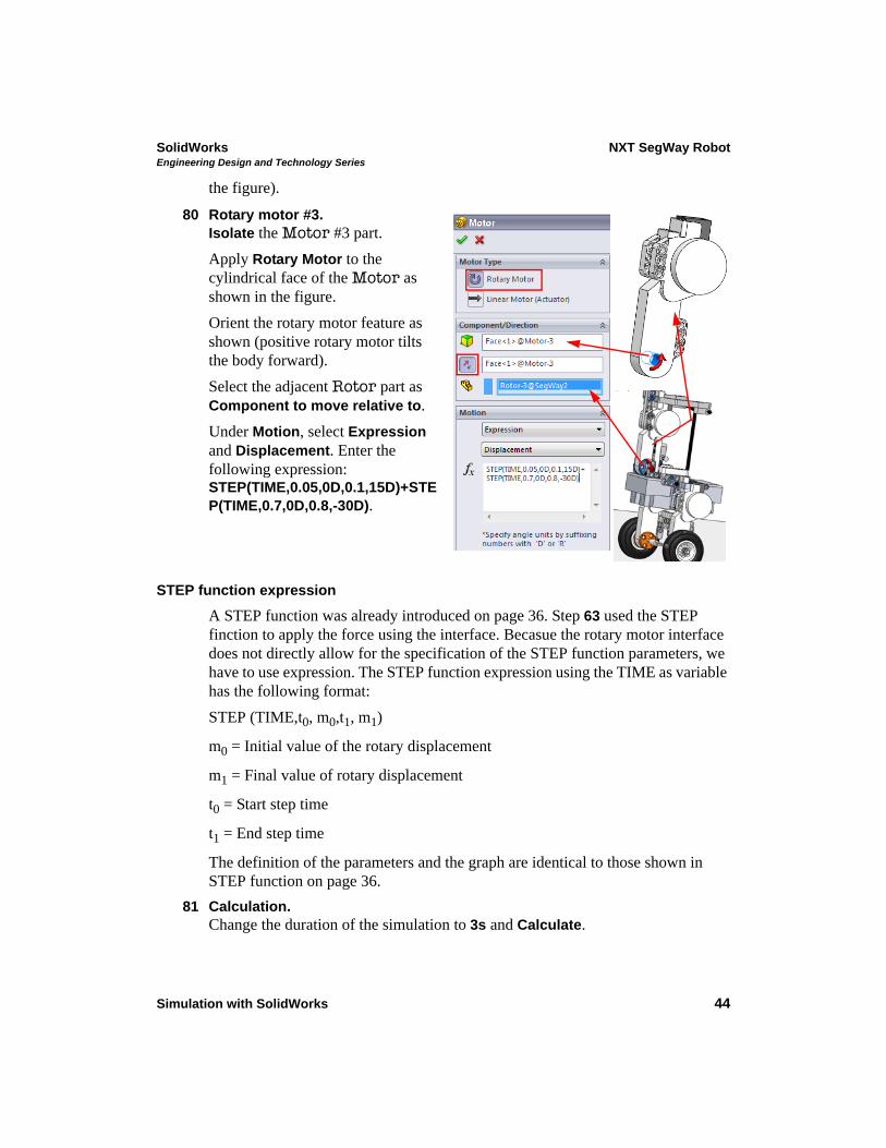
80 Rotary motor #3.Isolate the Motor #3 part.

Apply Rotary Motor to the cylindrical face of the Motor as shown in the figure.

Orient the rotary motor feature as shown (positive rotary motor tilts the body forward).

Select the adjacent Rotor part as Component to move relative to.

Under Motion, select Expression and Displacement. Enter the following expression: STEP(TIME,0.05,0D,0.1,15D)+STEP(TIME,0.7,0D,0.8,-30D).

STEP function expression

A STEP function was already introduced on page 36. Step 63 used the STEP finction to apply the force using the interface. Becasue the rotary motor interface does not directly allow for the specification of the STEP function parameters, we have to use expression. The STEP function expression using the TIME as variable has the following format:

STEP (TIME,t0, m0,t1, m1)

m0 = Initial value of the rotary displacement

m1 = Final value of rotary displacement

t0 = Start step time

t1 = End step time

The definition of the parameters and the graph are identical to those shown in STEP function on page 36.

81 Calculation.Change the duration of the simulation to 3s and Calculate.



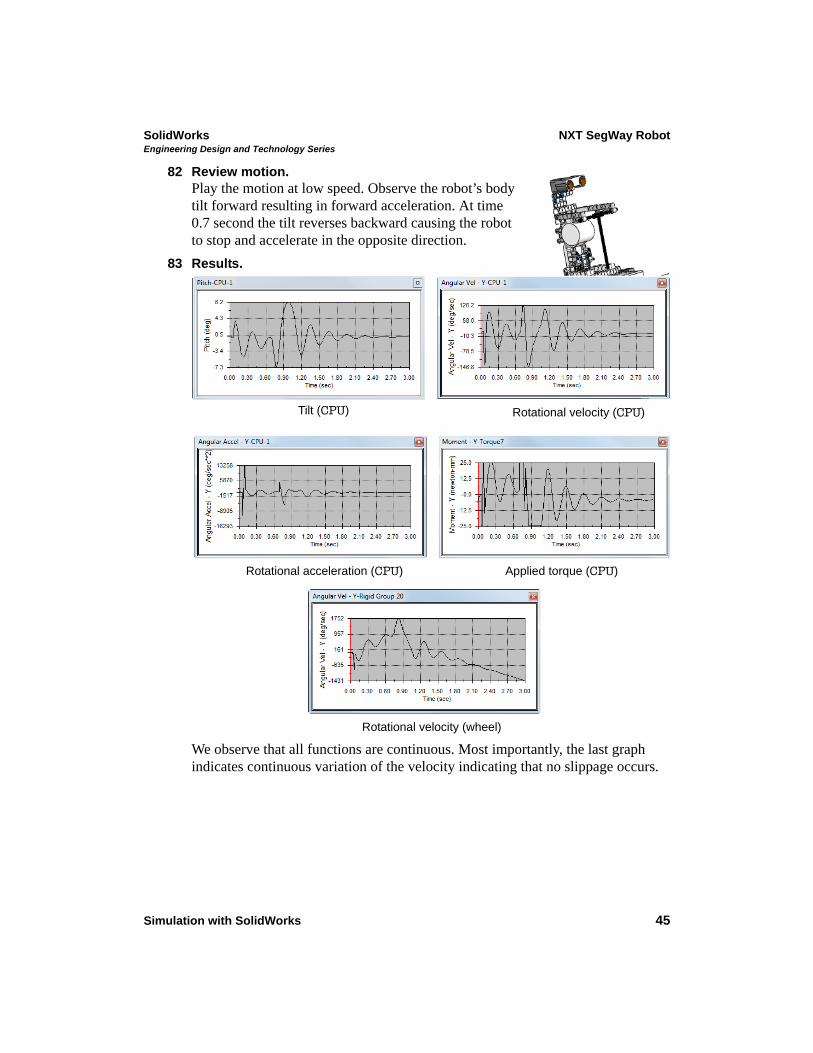
82 Review motion.Play the motion at low speed. Observe the robot’s body tilt forward resulting in forward acceleration. At time 0.7 second the tilt reverses backward causing the robot to stop and accelerate in the opposite direction.

83 Results.

We observe that all functions are continuous. Most importantly, the last graph indicates continuous variation of the velocity indicating that no slippage occurs.

Tilt (CPU) Rotational velocity (CPU)

Rotational acceleration (CPU) Applied torque (CPU)

Rotational velocity (wheel)

Documents

Lesson 1 NXT SegWay Robot - 3D CAD Design … Left and right side of the rider bottom. 7 Arms and chest. 8 Rider’s head. Left side Right side Left side Right side SolidWorks NXT