'LVNXVVLRQVSDSLHUH'LVFXVVLRQ�3DSHUV

'LVFXVVLRQ�3DSHU�1R�����

0RQH\�'HPDQG�LQ�(XURSH�(YLGHQFH�IURP�WKH�3DVW

E\(ONH�+DKQ���DQG�&KULVWLDQ�0�OOHU��

%HUOLQ��$SULO�����

���*HUPDQ�,QVWLWXWH�IRU�(FRQRPLF�5HVHDUFK��',:���%HUOLQ���+XPEROGW�8QLYHUVLW\��%HUOLQ

'HXWVFKHV�,QVWLWXW�I�U�:LUWVFKDIWVIRUVFKXQJ��%HUOLQ.|QLJLQ�/XLVH�6WU�����������%HUOLQ3KRQH� ���������������)D[� �����������������,QWHUQHW��KWWS���ZZZ�GLZ�GH,661����������

Money Demand in Europe:

Evidence from the Past �

Christian M�uller Elke Hahn

Institut f�ur Statistik und �Okonometrie Deutsches Institut

Sonderforschungsbereich 373 f�ur Wirtschaftsforschung

Humboldt{University Abteilung Konjunktur

Spandauer Str. 1 K�onigin-Luise-Str. 5

D-10178 Berlin, GERMANY D-14195 Berlin, GERMANY

Tel.: +49-30-2093-5717 Tel.: +49-30-89789-208

Fax: +49-30-2093-5712 Fax: +49-30-89789-102

Email: cmueller@wiwi.hu-berlin.de Email: ehahn@diw.de

Abstract

The conditions under which European monetary policy is likely to be conducted are investi-

gated by means of multi-variate time series modelling using aggregated data of all eleven European

Monetary Union member states. A cointegration analysis identi�es two stable long-run relation-

ships within a set of �ve key macroeconomic variables, one of which can be interpreted as a money

demand function and a second one as a long term real interest rate (Fisher parity). Our �ndings

indicate that monetary authorities might well be able to base their policy on the existence of a

money demand. Particular emphasis is given both to the data sources and their aggregation, by

providing a transparent account of our calculation procedure, which is not yet common in the

existing literature.

�We thank Helmut L�utkepohl, J�urgen Wolters and J�org Breitung for many helpful comments. We are indebted toKatja Rietzler for her support in constructing the GDP data. Of course, all mistakes are ours. Financial support fromthe Deutsche Forschungsgemeinschaft, SFB 373 is gratefully acknowledged.

1 Introduction

When the idea of a single currency for Europe won more and more followers, economists shifted the

focus of their research to the conditions under which a European monetary policy would likely have to

be conducted. One of the research interests focused on whether or not a European money demand is

stable and whether or not a more stable money demand on a European level compared with national

�ndings is a statistical artefact (see e.g. Arnold (1994), Artis, Bladen-Hovell and Zhang (1992) ).

By now there is widespread acceptance that European policy decisions have to be built upon the

data available so far, regardless of the impact of a possible change in agents behaviour which could

have been induced by the start of the European Monetary Union (EMU). Such a change in conditions

will only be apparent after some time. Therefore, from an empirical viewpoint, the best one can do is

to look at Europe as an economic union which, in principle, works like a large national economy.

For the �rst time Kremers and Lane (1990) estimated a European money demand by aggregating

national data sources. So far, most studies have focused on a limited set of countries, mainly the

larger or core countries of the EMU (see e.g. Wesche (1998), Hayo (1999), Monticelli and Strauss-

Kahn (1993) Fagan and Henry (1998) to name only a few). We estimate a money demand function

for the eleven EMU-countries. To our best knowledge only Gottschalk (1999) and Coenen and Vega

(1999) have chosen the same group of countries. In addition we present a detailled account of our

data sources and aggregation methods. Doing so we want to provide the most possible transparency

of our calculation procedure, which is not yet common in the literature.

The structure of the paper is as follows. We �rst discuss advantages and drawbacks of relying on

aggregated arti�cial data referring to the time prior to the European Monetary Union (EMU), then

outline in detail the data sources and aggregation methods we use to collect a data set for analyzing

money demand properties of the area of the EMU member states. We �nd it not reasonable to go

much further back in history than 1984 because data quality and availability deteriorates rapidly prior

to that date.

The second part of the paper is a cointegration analysis of money, income, long and short term

interest rates and prices within a Vector auto-regressive Error Correction Model (VECM) in order

to investigate the conditions for European monetary policy. The focus will be on long-run money

demand, which we are able to identify and, moreover, �nd to be stable.

A comparison with studies referring to the same set of countries, discussion of our �ndings and

of likely consequences for policy making as well as suggestions for an agenda for future research will

close the paper.

1

2 Special Problems concerning Aggregated Money Demand

Functions for the EMU

Economists who attempt to estimate a money demand function for the EMU are facing a number of

special problems. These have arisen because the EMU began just one year ago and so no long time

series data for it exists. One common solution is to rely on arti�cially constructed EMU data that

are generated by aggregating the national data of the participating countries for the time prior to the

EMU. In constructing these data one faces on the one hand problems with the availability and the

quality of the data used and on the other hand special problems concerning the appropriate aggregation

method. The issue of the availability and the quality of the data used is discussed in section 2.1 below.

The question of the appropriate aggregation method did not rise for our money demand investigation

because we used the oÆcial monetary aggregate for the EMU that was constructed by the European

Central Bank (ECB) itself. Paying attention to consistency when aggregating di�erent data series, we

constructed our other EMU series in the same way as the monetary aggregate. We therefore refrain

from conducting a detailed discussion of the advantages and disadvantages of di�erent aggregation

methods. Alongside this issue the interpretation of the results achieved with this arti�cial, aggregated

EMU data poses some special problems that are the subject of section 2.2.

2.1 Availability and Quality of the Data

Estimating a money demand for the EMU means estimating an aggregated money demand that

comprises the data of 11 countries.1 Providing suÆcient time series covering long periods for all

variables included in the money demand for all EMU countries turns out to be quite diÆcult especially

since the EMU area also comprises countries for which no extensive and detailed statistical data is

available. Therefore a considerable amount of estimation, particularly in the earlier part of our data

sample was unavoidable. The construction of the EMU data will be discussed in detail in section 3.2.

Furthermore, distortions in the EMU data are an important issue. Di�erent sources of impairment

can be identi�ed for the EMU data. Firstly they can be biased because the underlying national series

by themselves are distorted, for example, because of structural breaks. A second reason for distortion

in the aggregated data lies in the fact that this data often refers to non-harmonized national data.

The national time series are based on national data de�nitions which can vary signi�cantly between

countries. For instance di�erent calculation methods of Gross Domestic Product (GDP) or di�erent

maturities of the assets the interest rates refer to are underlying the aggregated EMU data. A further

harmonization problem arises because original, non-seasonally adjusted national data is not published

for all countries joining the EMU and di�erent procedures of seasonal adjustment are applied in

di�erent countries.

1These countries are Belgium, Spain, France, Ireland, Italy, Luxembourg, Austria, Netherlands, Portugal, Finlandand Germany.

2

2.2 Interpretation Problems

The interpretation of the results achieved with the arti�cial EMU data has to be taken with caution.

The question which arises is to how relevant the results and conclusions drawn from these arti�cial

data of the past are for the time period after the start of the EMU. Here it is essential to distinguish

between the relevance of the results based on past data for the time period after a potential structural

break in general and the relevance of the results referring to the arti�cially generated aggregated EMU

data for the time period after the start of the EMU in particular.

2.2.1 Inference for the EMU from Past Data

A general statement concerning the transferability of the results achieved before a regime shift to the

time period following the regime shift is related to the Lucas (1976) Critique . This implies that since

a regime shift like the introduction of the EMU and the start of a common monetary policy in the

EMU countries can induce changes in agents' behaviour, it is not compelling that conclusions drawn

on the basis of past data are valid also for the time period after the regime shift. Using this approach,

it follows that results obtained from our past aggregated EMU data for the money demand in the

EMU have to be interpreted carefully.

A potential source of a structural break in agents' behaviour is a change in the monetary conditions

present in the countries joining the EMU. The convergence process of monetary conditions of countries

participating in the EMU took place within the time period that underlies our investigation which

comprises the years from 1984 to 1998.2 This implies that a change in the behaviour of individuals

may have taken place within our estimation sample that could exert an in uence on money demand

and its stability properties. Against that, the monetary conditions at the end of our estimation sample

compare to those after the start of the EMU. Therefore a change in the behaviour of individuals at

the very day of the introduction of the Euro due to changing monetary conditions does not seem to

be likely. Subsequently the results obtained in our investigation should provide us with some evidence

about the conditions beyond that date.

Further arguments in favour of the relevance of the results based on past data for the EMU regime

are brought up by Hayo (1999). Firstly, he suggests that the economic shock on money demand

induced by the start of the EMU could possibly be only of temporary nature as was also often pointed

out for the shock brought about by the German monetary union. In this case monetary policy in the

EMU can rely on the results achieved on the basis of the past data. Secondly, he assumes that people

adjust their behaviour to the new monetary environment only very slowly. If this behavioral inertia

proves right, past experiences will be applicable to the EMU regime at least for some time.

2This can easily be seen by comparing, for instance, the in ation rates or the interest rates between the EMU countriesboth at the beginning and at the end of the period under consideration. At the beginning enormous di�erences showup while at the end convergence seems to be achieved.

3

2.2.2 Inferring from Aggregated Arti�cial EMU Data

Besides the general problems of transferring results achieved before a (potential) structural break to

the time after, evaluating the money demand and its properties in the EMU on the basis of arti�cially

aggregated data is accompanied by additional problems.

A special property of aggregated money demand functions seems to be that they exhibit better

stability properties compared to national functions.3 This leads to the question as to whether the

enhanced stability properties will be maintained after the start of the EMU, since EMU money demand

exerts in some way properties similar to national functions.

One possible explanation for the observed better stability properties of EMU money demand could

be that negatively correlated national shocks compensate each other. However, if this should prove

to be the reason for the enhanced stability properties, the stability of money demand is likely to

deteriorate after the start of the EMU since national shocks, especially monetary shocks, will occur

more synchronised within a monetary union.

The better stability properties of the aggregated EMU money demand could also be due to a

superior speci�cation of aggregated money demand functions compared to national functions. The

speci�cation bias caused by omitted variables such as currency substitution which constitutes a fre-

quent source of distortions for national money demand functions, is of minor importance for aggregated

money demand functions, since for larger areas foreign in uences are often included automatically.

For instance, for the aggregated EMU money demand the problem of currency substitution, as far

as it refers to European currencies, is solved solely for reasons of the new de�nition of the monetary

aggregate M3 of the ECB.

It is not clear, however, if the better stability properties of EMU money demand, that refer to a

superior speci�cation of EMU money demand, will remain after the EMU has began. Future instability

can certainly not arise from currency substitution between Euro countries yet may be introduced by

substitution between the EMU area and the rest of the world.

Furthermore the introduction of a single currency in Europe enhances competition between coun-

tries not only on the goods market by improving price transparency but also at the �nancial markets.

This spurs the development of �nancial innovations within the EMU, which could exert a negative

e�ect on the stability of money demand in the future as well (see Hayo (1999)).

All in all it is diÆcult to say if money demand and its properties are going to change in transition

to the EMU. While a number of arguments seem to indicate a change in individuals behaviour others

seem to reject it. In any case the results and conclusions taken on the basis of the past aggregated

data of the countries joining the EMU have to be interpreted with caution.

3See e.g. Kremers and Lane (1990), Monticelli and Strauss-Kahn (1993), Artis et al. (1992) and Monticelli (1996) infavour of that hypothesis and Arnold (1994) in opposition to it.

4

3 The Money Demand Function and the Data

This chapter is devoted to the speci�cation of the money demand function and the choice of variables

that should enter this function. Furthermore a detailed description of the construction features of the

aggregated data for the eleven EMU countries is given.

3.1 The Money Demand Function

In empirical investigations on money demand usually the demand for real money is estimated. There

are two reasons which imply the speci�cation of demand for real money. The �rst relies on economic

theory; money is in general supposed to be neutral in the long run, consequently long run price

homogeneity is assumed. The second reason is based on econometric grounds. In most econometric

investigations nominal money stock as well as the price level are found to be not only non stationary

but even I(2). In line with these results lies the fact that the demand for real money usually shows up

as I(1), i.e. a cointegration relationship between nominal money demand and the price level exists. As

econometric modelling with I(1) variables is supposed to be easier than with I(2) variables, estimating

the demand for real money is generally preferred and will also be applied in this paper.

Economic theory suggests di�erent reasons for holding money. Two main purposes for holding

money can be distinguished. On the one hand money is held for transaction purposes. On the other

hand holding money is part of the optimal portfolio selection. In our money demand speci�cation

we use a broad monetary aggregate since the ECB decided to target the broad monetary aggregate

M3. The transaction motive of holding money is represented by real GDP. A long term interest

rate, a short term interest rate and the in ation rate are added as portfolio choice variables. The

long term interest rate measures the rate of return to �nancial assets not included in the monetary

aggregate whereas the short term interest rate can be interpreted as a proxy of the own rate of return

{ this concept is consistent with the employed broad monetary aggregate { and at the same time as

a policy variable. Alternatively, the interest rate spread could be applied to model the opportunity

costs of holding money compared with other �nancial assets. Furthermore, the in ation rate re ects

the opportunity costs of holding money contrary to holding real assets.

Equation (1) comprises our speci�cation of the long-run money demand function.

Md=P = f(Y; il; is; �) (1)

Md; P; Y; il; is; � represent the nominal money demand, the price level, the real GDP, the long term

interest rate, the short term interest rate and the in ation rate respectively. For a better interpretation

of the estimated coeÆcients, a log-linear form of the money demand function is applied as illustrated

in equation (2)

(m� p) = �yy + �il il + �is i

s + ��� + ecm (2)

5

where lower casesm; p; y indicate logarithms, while the interest rates are expressed in levels. The error

correction term is denoted ecm. The coeÆcient �y represents the income elasticity of the demand for

money. It should show a positive sign; as income increases so does the transaction demand for money.

Corresponding to the quantity theory this elasticity should equal unity, while the Baumol-Tobin theory

of money demand suggests a coeÆcient of 0.5. Conversely in other empirical investigations on the

demand for broad money the coeÆcient often exhibits a value that exceeds unity. This value compares

to the observation of a trend decline in the velocity of circulation. It can be explained by �nancial

innovations and wealth e�ects, which are not explicitly modelled. Higher wealth leads according to

the optimal portfolio selection to higher investment in all assets including those short term assets that

are part of the money demand.

The coeÆcient �is re ects the semi-elasticity of money with respect to the short term interest

rate. This coeÆcient should exhibit a positive sign since a higher rate of return of the short term

assets included in the monetary aggregate increases their attractiveness compared to other assets. On

the contrary, an increase in the long term interest rate induces portfolio shifts towards longer term

investments, which reduces the demand for money and corresponds to a negative sign of �il , the semi-

elasticity of money with respect to the long term interest rate. If the coeÆcients �il and �is have the

same magnitude and opposite signs, they can be interpreted as the opportunity costs of holding money

compared to other �nancial assets, which constitutes an alternative modelling possibility. The semi-

elasticity of money with respect to the in ation rate, ��, should show up as negative since an increase

in the in ation rate reduces the value of monetary assets. The in ation rate therefore represents the

rate of return of real assets compared to nominal assets.

3.2 The Data

The estimation and test results are sensitive to the construction of the data in general and the employed

aggregation method in particular. Therefore the construction and aggregation procedure of the EMU

data underlying this investigation is an important feature and is described precisely in the following.4

The analysis is based on quarterly data that refers to the time period from 1984(1) to 1998(2). To

cater for lags and di�erenced variables the estimation sample starts at 1985(1).

The monetary aggregate used in this paper is the oÆcial aggregate M3 of the ECB. A historical

time series of this data was published by European Central Bank (1999). The de�nition of the

monetary aggregate M3 of the ECB corresponds to a very broad monetary aggregate; it is broader

than the aggregate M3 that was used previously for example by the German Bundesbank.5 As the

ECB implemented a new de�nition for M3, that contains di�erent and new components such as

4 An exact overview of the national data sources and of the time periods for which national data is estimated as wellas the applied estimation methods, is given in the Tables 9 to 13 in Appendix B respectively.

5The monetary aggregate M3 of the ECB comprises currency in circulation, overnight deposits, deposits with agreedmaturity up to 2 years, deposits redeemable at notice up to 3 months, repurchase agreements, money market fundshares/units and money market paper and debt securities up to 2 years.

6

money market funds and money market paper \a considerable amount of estimation was necessary,

particularly for earlier dates" (European Central Bank (1999), p. 41). Furthermore, the ECB adjusted

the national series for important structural breaks. For example, the impact of the German uni�cation

was straightened out of the time series. The national M3 series were then converted into Euro by

the ECB using the irrevocably �xed conversion rates vis-�a-vis the Euro which were determined on 31

December 1998. Thereafter the national series were added up. The M3 data was published as non-

seasonally adjusted end-of-month data. We transformed the end-of-month data into end-of-quarter

data by using the last month of each quarter as quarterly data. Afterwards the M3 data was seasonally

adjusted applying Berlin Method (BV4).6 Seasonal adjustment of M3 had to be applied for reasons

of a consistent data set (see GDP construction below).

The main data source for the national real and nominal GDP data is Eurostat. We calculated

real and nominal GDP, because the increase of the resulting implicit GDP de ator serves as an

in ation rate. In periods where no national data was available estimations had to be carried out. If,

for example, during a certain period Eurostat data for one country was missing, but data from the

Organisation for Economic Cooperation and Development (OECD) was available, then we calculated

the level of the Eurostat GDP data in the missing period using the growth rate of the OECD data.

The national data relies on the European System of Accounts going back to 1979 (ESA 79) because

for the harmonized and therefore more appropriate European System of Accounts after the convention

of 1995 (ESA 95) no long time series are at hand. Furthermore, for some countries, such as France,

only seasonally adjusted GDP data exists. Therefore we decided to use seasonally adjusted GDP data

for all countries.

In analogy to the calculation of the monetary aggregate M3 by the ECB we adjusted the GDP

series for the impact of the German reuni�cation. The GDP data series for uni�ed Germany which

is applied in our analyses starts in 1989(1). Before that date no such data is available. We therefore

estimated the GDP data for Germany for the period before 1989(1) assuming the growth rates of the

West German GDP data. We then transformed the national GDP series into Euro currency using the

�xed conversion rates vis-�a-vis the Euro. After aggregating the national GDP series we obtained our

EMU-GDP time series.

The national data of the long and short term interest rates are taken from the OECD Main

Economic Indicators. The long term interest rates represent the yield of long term government bonds.

Unfortunately, the rates of return of the government bonds published by the OECD for di�erent

countries do not re ect exactly the same maturities. For example, for Germany the yield on public

sector bonds with 7 to 15 years duration is taken while for Italy the yield on treasury bonds of maturity

of one year or more is included.

Against that, the short term interest rates refer exactly to the same maturities in all countries.

6BV4 is the abbreviation of the German name Berliner Verfahren Version Nummer 4 which stands for Berlin Methodversion number 4. See Nourney (1993) for a description.

7

They measure the yield of three-month inter bank deposits which is represented for instance in Ger-

many by the three-month FIBOR or in France by the three-month PIBOR. The national interest rate

series are constructed as end-of-quarter data. They are weighted with their current share of EMU-

GDP to obtain the EMU interest rate series. In years where no interest rate data for a particular

country was available the interest rate of this country does not enter into the calculation. The in ation

is measured as quarter on quarter increase of the GDP de ator.

4 Cointegration Analysis

In this chapter a cointegration analysis is carried out. After analysing the stationarity properties

of our variable set, we will discuss our general modelling approach, then turn to determining the

cointegrating rank of our system and �nally, try to identify the cointegration vectors as well as their

stability properties.

4.1 Data Properties

Knowledge about the stationarity properties of the data underlying the investigation is crucial to the

choice of the appropriate econometric methods. Therefore, in a �rst step we conducted unit root

tests for the �ve variables under consideration to discriminate between trend stationary and di�erence

stationary variables.

From the results achieved with the Augmented-Dickey-Fuller (ADF) tests and the Phillips Perron

(PP) tests shown in Table 1 we conclude that all variables are non-stationary (or to be more precise

integrated of order one, I(1)).7 Visual inspection of the time series shown in Figure 2 in the data

appendix seems to support our conclusions.

4.2 The General Model

Following the considerations outlined previously, we investigate a very general macro-economic model

by means of a vector auto-regressive process of the form

Xt = D +

kX

i=1

AiXt�i +Et (3)

where Xt is a (n � T ) matrix of our n variable series (x = [(m � p) y il is 4p]0) with T = 54

observations each. Et is a vector of error terms assumed to be distributed Et � (0;�). The vector

D collects the constant terms. Economic structure enters the setup when the sample of integrated

variables exhibits cointegration features such as for example in equation (2). That means �nding

long-run relationships between the variables we will have to check whether or not they comply to the

7Calculations were performed with the software packages PcF iml (see Doornik and Hendry (1997)), GAUSS andEViews 2.0.

8

Table 1: Unit root tests (1985(1) - 1998(2))

Variable NotationADF Test+ PP Test 5 Percent

DecisionSetup++ Statistic Setup++ Statistic Crit. Val.+++

log(M3=P ) m� p c,t,1,3,4,5 -1.51 c,t,3 -0.91 -3.50 I(1)

4log(M3=P ) c,3,4 -2.57 c,3 -3.86� -2.91

log(GDP ) y c,t,1,2 -2.09 c,t,3 -1.64 -3.50 I(1)

4log(GDP ) c,1,4 -2.42 c,3 -5.04� -2.91

il il c,1 -1.11 c,3 -0.75 -2.91 I(1)

4il c,1,5 -4.08� c,3 -4.53� -2.91

is is c,1 -1.05 c,3 -0.91 -2.91 I(1)

4is c -5.29� c,3 -5.18� -2.91

4log(P ) 1

4� c,1,4 -1.19 c,3 -2.30 -2.91 I(1)

42log(P ) c,2 -11.19� c,3 -11.29� -2.91

il � is c,1,4 -2.50 c,3 -1.89 -2.91 I(1)

4(il � is) c,3 -5.84� c,3 -5.96� -2.91

is � 44p c -2.32 c,3 -2.24 -2.91 I(1)

4(is � 44p) c -9.22� c,3 -9.21� -2.91

il � 44p c -3.64� c,3 -3.74� -2.91 I(0)

� indicates signi�cance at the �ve percent level+ The sample size had to be adjusted according to the setup in some cases.++ c: constant, t: trend, the integers indicate the lags of di�erenced dependent

variables included in the regression (ADF test) and the truncation lag (PP test)+++ MacKinnon (1991) critical values

concept of money demand for example. We therefore turn to a cointegration analysis in the Johansen

reduced rank framework by rewriting (3) to obtain

4Xt = �+�Xt�1 +k�1X

i=1

�i4Xt�i +Et (4)

with 4 = (1 � L) and L being the lag or backshift operator (LXt = Xt�1). For details of the

relationship between the Ai, D and �; �;� matrices see e.g. L�utkepohl (1993). The interesting term

on the r.h.s of (4) is the matrix � which has reduced rank if the variables are cointegrated. This matrix

� potentially contains information about long-run relationships of the variables under consideration.

We now investigate its properties.

4.3 Determination of the Cointegrating Rank

From a theoretical perspective three linearly independent cointegration relationships could have been

expected. Next to a stationary money demand function theory suggests the interest rate spread as

well as the real interest rates might prove to be stationary. The assumption of a stationary spread is

derived from the expectation hypothesis of the term structure. According to this hypothesis the long

term interest rate is determined by the average of the present and the expected future short term

interest rates. Therefore, except for a risk premium8, the yield of the longer term investment should

8Economic theory suggests this premium to be stationary.

9

equal the yield of several short term investments that together cover the same period. Finally, the

idea of stationary real interest rates refers to the Fisher parity, which explains the frequently observed

positive correlation between interest rates and the in ation rate. Higher in ation reduces the real

yield of nominal assets compared to real assets which via higher demand for credits induces nominal

interest rates to increase. We keep in mind these theoretical proposals for the potential cointegration

relationships when we now turn to the determination of the actual cointegrating rank of our system.

Noting the dependence of the performance of cointegration tests on the number of observations

available we not only perform one test at a certain lag length but also vary the number of lagged

endogenous variables and consider subsystems.9 That is, starting with a maximum lag length of

three, which seems to be reasonable given 58 observations (54 observations from 1985(1) to 1998(2)

and four pre-sample data points) in our sample and �ve variables under investigation, we reduce the

number of lags down to one and do so for three models. These are the full model (�ve variables), a

model which excludes in ation and a third, which consists of real money, income and the long term

interest rate only.

Table 2 reports the cointegrating ranks chosen in a sequential test procedure by three di�erent tests

at the �ve and ten percent level of signi�cance. The three tests are the well known Johansen (1995)

likelihood-ratio test (LRJ , trace statistic), another LR test with trend adjustment and a maximum

likelihood (LM) type test, both of which have been suggested by L�utkepohl and Saikkonen (2000).

The relative performance of all these tests has been analysed e.g. by Hubrich et al. (1998). In Table

2 it can be seen that the cointegrating rank of the full system seems to be two. At lag length two for

example, there is unanimous evidence in favour of that, although at the ten percent level only for the

Johansen test. The corresponding test results for lag order two are given in Table 5 in the appendix

A. When the in ation variable (4p) is excluded, all tests report in most cases one cointegrating rank

only. Almost no evidence in support of any cointegration is found when a system of money, income

and a long term interest rate is considered. When evaluating the test results one should have in mind

that the loss in power often becomes substantial when the degrees of freedom are rather low, which

is the case with the current sample at lag length three already (�ve and four variables). The size, on

the other hand, often tends to exceed its nominal level if the true lag length has been understated.

Fortunately, our experiment gives a relatively consistent picture, that is, the full system is coin-

tegrated of order two, where one of the cointegration relationships requires inclusion of the in ation

variable and the second includes money, income and possibly long and short term interest rates.

Therefore, from an economists point of view we expect one relationship relating money to income and

probably interest rates and a second one might link e.g. long term interest rates and in ation to yield

some stationary real interest rate.

9See Reimers (1991), Yap and Reinsel (1995), Saikkonen and Luukkonen (1997) and Hubrich, L�utkepohl and Saikko-nen (1998) on the properties of cointegration tests with varying lag order and dimension. A general outcome is theremarkable deterioration of power when the lag length and/or dimension of the system becomes larger.

10

Table 2: Cointegration Test: Ranks selected by various tests�

4Xt = �+ ��0Xt�1 + �k�1

i=1�i4Xt�i + Et

k LRJ LRta LM(r0)(it)

X0 = ((m � p); y; il; is;4p) full model

1 1 (2) 1 1

2 1 (2) 2 2

3 1 2 1

X0 = ((m � p); y; il; is) in ation excluded

1 1 (2) 1 1

2 1 1 0

3 0 0 0

X0 = ((m � p); y; il) basic money demand

1 0(1) 1 0

2 0(1) 0 0

3 0 0 0

� The columns report the ranks selected at the 5 % level of signi�cance and

at the 10% level in brackets if there is a di�erence.

A sequential test procedure and trace statistics are applied.

LRta refers to a Johansen like test on the adjusted series ~x in

L�utkepohl and Saikkonen (2000), p.184. LM(r0)(it) refers to

L�utkepohl and Saikkonen (2000), eq. 4.10, two-step procedure

for estimating �0 and �1, it indicates iterative variant.

Before turning to the actual identi�cation of the cointegration matrix a note on the choice of

the lag length is in order. Starting again at a maximum length of three we perform F-tests of

parameter reduction and apply order selection criteria. While the Schwarz Criterion (SC), Hannan-

Quinn Criterion (HQ) and Akaike Information Criterion (AIC) all point to di�erent lag lengths, the

F-tests imply that a reduction from three to two lags, yet not further, is acceptable (see Tables 6

and 7 in the appendix A). We therefore continue the analysis with two lags, a decision which also

�nds support from a number of speci�cation tests, almost none of which indicate serious problems

(Table 8). Working with two lags (k = 2) in the VAR representation of equation (3) also ensures a

parsimonious parametrisation.

4.4 Identi�cation of Cointegration Vectors

In this section, the cointegration relationships are to be identi�ed. Out of the three hypothesized

cointegration relationships, the interest rate spread has already been found to be non stationary but

the long term real rate seems to be stationary (see Table 1). In the following we will refer to this

result.

Determining the cointegration vectors we make use of the reduced rank property of the cointegrat-

ing matrix, namely that it can be separated into two matrices of full column rank as it has become

common procedure since Johansen (1988). We de�ne ��0 = � with � and � of dimension (n� 2) and

11

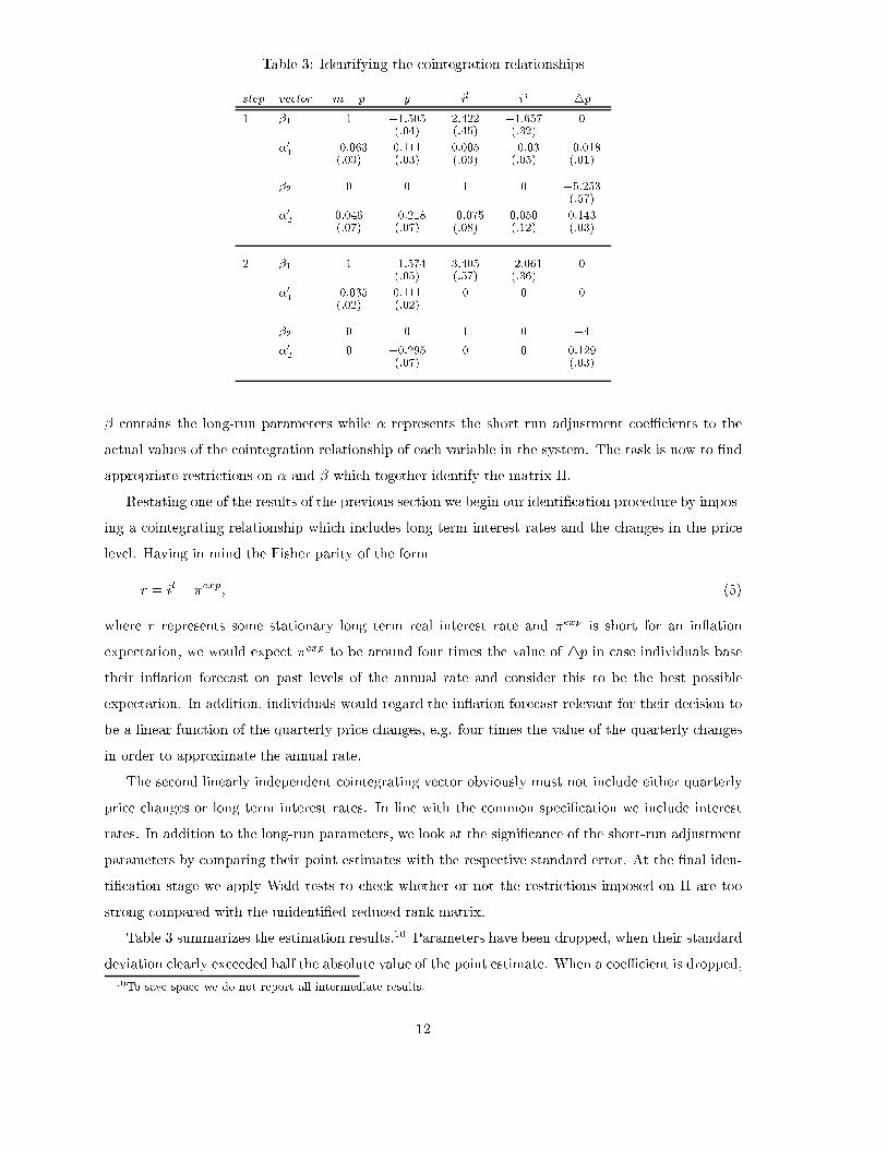
Table 3: Identifying the cointegration relationships

step vector m� p y il is 4p

1 �1 1 �1:505(:04)

2:422(:45)

�1:657(:32)

0

�01

�0:063(:03)

0:111(:03)

0:005(:03)

�0:03(:05)

�0:018(:01)

�2 0 0 1 0 �5:253(:57)

�02

0:046(:07)

�0:218(:07)

�0:075(:08)

0:050(:12)

0:143(:03)

2 �1 1 �1:574(:05)

3:405(:57)

�2:061(:36)

0

�01

�0:035(:02)

0:111(:02)

0 0 0

�2 0 0 1 0 �4

�02

0 �0:295(:07)

0 0 0:129(:03)

� contains the long-run parameters while � represents the short run adjustment coeÆcients to the

actual values of the cointegration relationship of each variable in the system. The task is now to �nd

appropriate restrictions on � and � which together identify the matrix �.

Restating one of the results of the previous section we begin our identi�cation procedure by impos-

ing a cointegrating relationship which includes long term interest rates and the changes in the price

level. Having in mind the Fisher parity of the form

r = il � �exp; (5)

where r represents some stationary long term real interest rate and �exp is short for an in ation

expectation, we would expect �exp to be around four times the value of 4p in case individuals base

their in ation forecast on past levels of the annual rate and consider this to be the best possible

expectation. In addition, individuals would regard the in ation forecast relevant for their decision to

be a linear function of the quarterly price changes, e.g. four times the value of the quarterly changes

in order to approximate the annual rate.

The second linearly independent cointegrating vector obviously must not include either quarterly

price changes or long term interest rates. In line with the common speci�cation we include interest

rates. In addition to the long-run parameters, we look at the signi�cance of the short-run adjustment

parameters by comparing their point estimates with the respective standard error. At the �nal iden-

ti�cation stage we apply Wald tests to check whether or not the restrictions imposed on � are too

strong compared with the unidenti�ed reduced rank matrix.

Table 3 summarizes the estimation results.10 Parameters have been dropped, when their standard

deviation clearly exceeded half the absolute value of the point estimate. When a coeÆcient is dropped,10To save space we do not report all intermediate results.

12

its value is set to zero, in this case as well as in the cases where parameters serve scaling purposes or

are set to equal certain values, no standard deviation is reported.

In the �rst step one relationship is de�ned such that it may re ect a money demand function

and the other possibly represents the Fisher parity. Therefore in the �rst vector changes in prices

are excluded while in the second, only the coeÆcients on long term interest rates and the change

in prices are estimated. As a result the �rst relationship's estimates are convincingly in line with a

money demand function. This is true with respect to both the sign and magnitude of the parameter

estimates. In addition they all seem to be statistically signi�cant. The second relationship yields a

coeÆcient on price changes of �5:25 being not very far from the �4 which is to be expected following

the discussion above.

Finally, we set a number of adjustment parameters to zero according to the criteria mentioned

above. Additionally we restricted the parameter of the in ation variable in the "Fisher equation" to

�4 and performed a Wald test on whether or not all the restrictions imposed in the second step are

statistically signi�cant. The corresponding �2 statistic with 9 degrees of freedom yields 14:49 with a

marginal probability of 11%.

Hypothesising this outcome to be robust throughout time, we recursively estimated the parameters

of � and � except from those which had been previously restricted. We do not �nd evidence of either

instability of the long-run coeÆcients or of rejection of the restrictions at any point in time between

1992(4) and 1998(2). To demonstrate this property in Figure 1 we provide a graphical analysis by

collecting the recursive estimation results for the freely estimated coeÆcients and the Wald statistic,

together with the estimated cointegration relationships as well as the eigenvalues of the unrestricted

system.

We conclude

m� p = 1:574y � 3:405il + 2:061is and (6)

il = 44p (7)

to be valid and stable restrictions of the cointegration space representing stationary relationships of the

non-stationary data. The �rst of them (6) may well be interpreted as a money demand relationship

in line with (2). Here, the income elasticity is nearly 1:6 being consistent with a trend decline of

the velocity of circulation in a monetarist framework. Interest rates either induce money holdings to

decrease when the opportunity costs, measured by the long term rates, increase, or to expand when

assets inside the broad monetary aggregate promise higher returns. The respective coeÆcients are

of similar magnitude, although money seems to be more sensitive with respect to long term interest

rates.

A stationary interest rate spread as proposed by the expectation theory of the term structure could

not be identi�ed within our system, although the graphical analysis of the interest rates (see Figure

2 in the appendix B) points to the direction that the expectation theory could hold. The lack of a

13

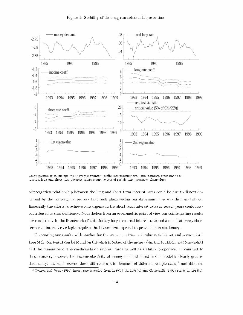
Figure 1: Stability of the long-run relationship over time

1985 1990 1995

-2.85

-2.8

-2.75money demand

1993 1994 1995 1996 1997 1998 19990.2.4.6.81 1st eigenvalue

1993 1994 1995 1996 1997 1998 1999-2

-1.8

-1.6

-1.4

-1.2income coeff.

1993 1994 1995 1996 1997 1998 199902468 long rate coeff.

1993 1994 1995 1996 1997 1998 1999-6

-4

-2

0short rate coeff.

1985 1990 1995

.04

.06

.08 real long rate

1993 1994 1995 1996 1997 1998 19990.2.4.6.81 2nd eigenvalue

1993 1994 1995 1996 1997 1998 19995

10

15

20rec. test statisticcritical value (5% of Chi^2(9))

Cointegration relationships; recursively estimated coeÆcients together with two standard error bands onincome, long and short term interest rates; recursive test of restrictions; recursive eigenvalues

cointegration relationship between the long and short term interest rates could be due to distortions

caused by the convergence process that took place within our data sample as was discussed above.

Especially the e�orts to achieve convergence in the short term interest rates in recent years could have

contributed to that de�ciency. Nonetheless from an econometric point of view our cointegrating results

are consistent. In the framework of a stationary long term real interest rate and a non-stationary short

term real interest rate logic requires the interest rate spread to prove as non-stationary.

Comparing our results with studies for the same countries, a similar variable set and econometric

approach, consensus can be found on the general outset of the money demand equation, its components

and the dimension of the coeÆcients on interest rates as well as stability properties. In contrast to

these studies, however, the income elasticity of money demand found in our model is clearly greater

than unity. To some extent these di�erences arise because of di�erent sample sizes11 and di�erent

11Coenen and Vega (1999) investigate a period from 1980(1) till 1998(4) and Gottschalk (1999) starts at 1983(1),

14

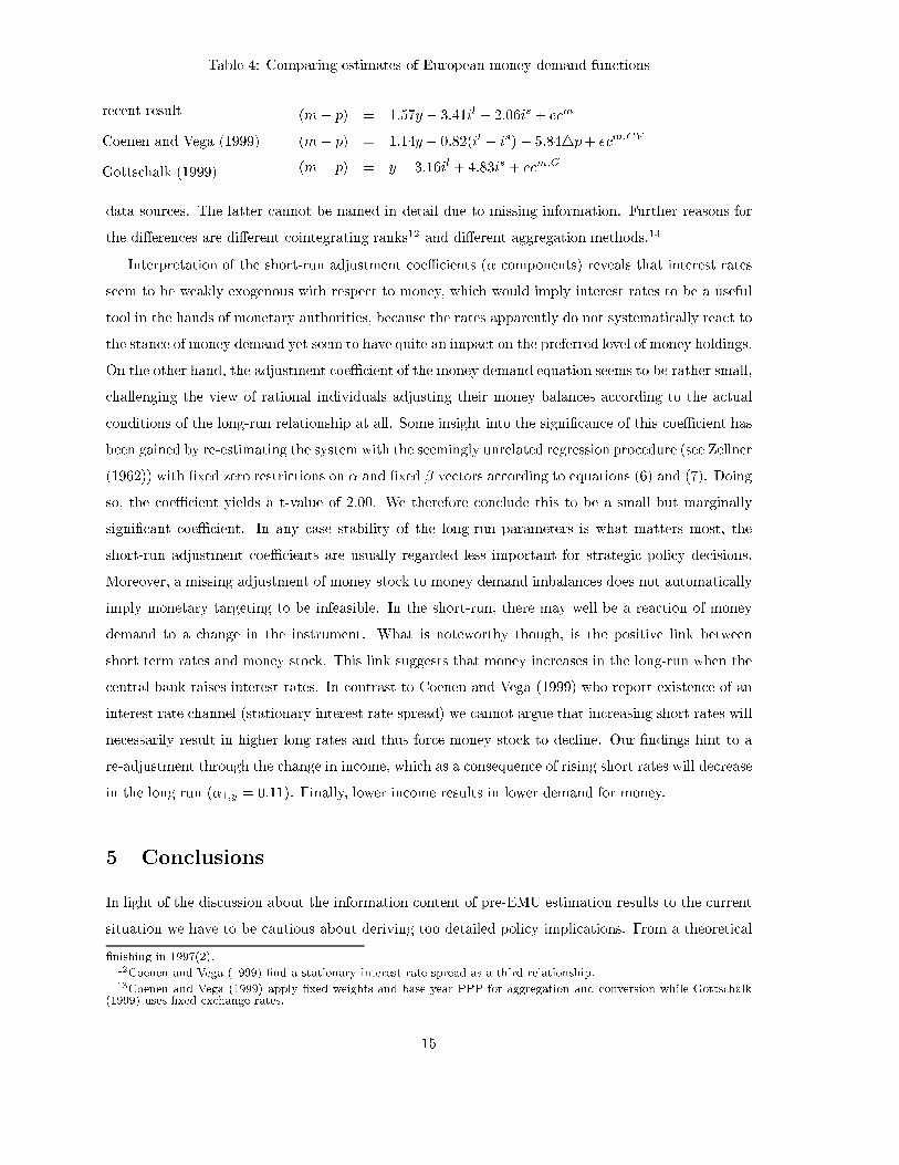
Table 4: Comparing estimates of European money demand functions

recent result

Coenen and Vega (1999)

Gottschalk (1999)

(m� p) = 1:57y� 3:41il + 2:06is + ecm

(m� p) = 1:14y� 0:82(il � is)� 5:844p+ ecm;CV

(m� p) = y � 3:16il + 4:83is + ecm;G

data sources. The latter cannot be named in detail due to missing information. Further reasons for

the di�erences are di�erent cointegrating ranks12 and di�erent aggregation methods.13

Interpretation of the short-run adjustment coeÆcients (� components) reveals that interest rates

seem to be weakly exogenous with respect to money, which would imply interest rates to be a useful

tool in the hands of monetary authorities, because the rates apparently do not systematically react to

the stance of money demand yet seem to have quite an impact on the preferred level of money holdings.

On the other hand, the adjustment coeÆcient of the money demand equation seems to be rather small,

challenging the view of rational individuals adjusting their money balances according to the actual

conditions of the long-run relationship at all. Some insight into the signi�cance of this coeÆcient has

been gained by re-estimating the system with the seemingly unrelated regression procedure (see Zellner

(1962)) with �xed zero restrictions on � and �xed � vectors according to equations (6) and (7). Doing

so, the coeÆcient yields a t-value of 2:00. We therefore conclude this to be a small but marginally

signi�cant coeÆcient. In any case stability of the long-run parameters is what matters most, the

short-run adjustment coeÆcients are usually regarded less important for strategic policy decisions.

Moreover, a missing adjustment of money stock to money demand imbalances does not automatically

imply monetary targeting to be infeasible. In the short-run, there may well be a reaction of money

demand to a change in the instrument. What is noteworthy though, is the positive link between

short term rates and money stock. This link suggests that money increases in the long-run when the

central bank raises interest rates. In contrast to Coenen and Vega (1999) who report existence of an

interest rate channel (stationary interest rate spread) we cannot argue that increasing short rates will

necessarily result in higher long rates and thus force money stock to decline. Our �ndings hint to a

re-adjustment through the change in income, which as a consequence of rising short rates will decrease

in the long run (�1;y = 0:11). Finally, lower income results in lower demand for money.

5 Conclusions

In light of the discussion about the information content of pre-EMU estimation results to the current

situation we have to be cautious about deriving too detailed policy implications. From a theoretical

�nishing in 1997(2).12Coenen and Vega (1999) �nd a stationary interest rate spread as a third relationship.13Coenen and Vega (1999) apply �xed weights and base year PPP for aggregation and conversion while Gottschalk

(1999) uses �xed exchange rates.

15

point of view the question has to be raised as to what extent the convergence process for the EMU

in uences our estimation results. This might be a more serious problem with respect to the short term

adjustment estimates (�; �i coeÆcients, equation (4)) than for the long-run relationships identi�ed.

The stability analysis on the one hand investigates the impact of new information being available while

approaching the Euro date. It is therefore fair enough to conclude that, since nothing has changed

signi�cantly in that period, the relationships we are interested in are stable. On the other hand,

however, the �nal estimation results might be too much distorted by very early observations which

are allowed to have the same impact as the more recent one. There is certainly no easy solution to

control for this.

Noting the discrepancy between short and long-run adjustment coeÆcients (�; �i versus � in

equation (4)) in terms of the rate of convergence we do not yet push the analysis beyond the long-run

investigation.14 We would be ready to do so, however, if two very principal conditions are ful�lled.

The �rst one is to �nd an appropriate estimation scheme that accounts for the adjustments made in

preparation for the Euro. This could be done for example by weighing earlier observations less when

across country variability e.g. of in ation rates is high or by estimating panel data models. The latter

unfortunately does not seem to be promising due to an apparent imbalanced proportion between both

the number of reliable data points and their respective parameters which have to be estimated.

The second condition is stability of all the short-run coeÆcients e.g. because the actual shape of

impulse response curves depend on these coeÆcients as well.

To sum up, before the diÆcult background of analysing aggregated data we �nd two stable long-run

relationships within a set of variables comprising a broad monetary aggregate, real income, long and

short term interest rates and prices. One of these relationships is in line with the long-run real interest

rate (Fisher parity) whereas the second implies the existence of a stable money demand at the EMU

level. The coeÆcients of the long-run money demand compare favourably with those of other studies,

except for the income elasticity of money demand. Its magnitude of 1:6 exceeds unity considerably.

We relate this �nding to the trend decline in the velocity of circulation. Although apparently small,

adjustment of money to deviations from the long-run money demand equilibrium seems to take place.

Moreover interest rates are weakly exogenous and can therefore, in the longer run be used for policy

making such as targeting money.15

We have tested the stability of the long-run parameters along with the weak exogeneity properties

and have found them to be stable over a period of almost six years before the start of the EMU. Our

�ndings provide no evidence against monetary targeting as applied by the ECB as one of the two

pillars of its monetary strategy.

14This could be done by impulse-response analysis for example to model the impact of policy measures as in Coenenand Vega (1999).15See Ericsson (1999) for a discussion of weak exogeneity implications.

16

References

Arnold, I. J. (1994). The Myth of a Stable European Money Demand, Open Economics Review 5: 249

{259.

Artis, M. J., Bladen-Hovell, R. C. and Zhang, W. (1992). A European Money Demand Function, in

P. R. and M. P. Taylor (eds), Policy Issues in the Operation of Currency Unions, International

Monetary Fund.

Coenen, G. and Vega, J.-L. (1999). The Demand for M3 in the Euro Area,Working Paper 6, European

Central Bank.

Doornik, J. A. and Hendry, D. F. (1997). PcFiml 9.0. A module for econometric modelling of dynamic

systems.

Ericsson, N. (1999). Empirical modelling of money demand, in H. L�utkepohl and J. Wolters (eds),

Money Demand in Europe, Physika-Verlag, Heidelberg, pp. 29 { 49.

European Central Bank (1999). Monthly Bulletin February, European Central Bank.

Fagan, G. and Henry, J. (1998). Long run money demand in the EU: Evidence for area wide aggregates,

Empirical Economics 23(3): 483 506.

Gottschalk, J. (1999). A Cointegration Analysis of a Money Demand System in Europe, Kiel Working

Paper 902, The Kiel Institute of World Economics.

Hayo, B. (1999). Estimating A European Demand for Money, Scottish Journal of Political Economy

46(3): 221{44.

Hubrich, K., L�utkepohl, H. and Saikkonen, P. (1998). A Review of Systems Cointegration

Tests, Discussion Paper 101, Sonderforschungsbereich 373 at Humboldt-Universit�at zu Berlin,

http://sfb.wiwi.hu-berlin.de/cgi-bin/sfb/read.pl?jahr=1998.

Johansen, S. (1988). Statistical Analysis of Cointegration Vectors, Journal of Economic Dynamics

12: 231 { 54.

Johansen, S. (1995). Identifying restrictions of linear equation with applications to simultaneous

equations and cointegration, JOEM 69: 111 { 132.

Kremers, J. and Lane, T. (1990). Economic and Monetary Integration and the Aggregate Demand

for Money in the EMS, Sta� Paper 37, International Monetary Fund.

Lucas, R. E. (1976). Econometric policy evaluation: A critique, Carnegie Rochester Conferences on

Public Policy 1, pp. 19 { 46.

17

L�utkepohl, H. (1993). Introduction to Multiple Time Series Analysis, 2nd edn, Springer-Verlag, Berlin.

L�utkepohl, H. and Saikkonen, P. (2000). Testing for the cointegrating rank of a VAR process with a

time trend, Journal of Econometrics 95: 177{198.

MacKinnon, J. (1991). Critical Values for co-integration tests, in R. Engle and C. Granger (eds),

Long-Run Economic Relationships, Oxford University Press, Washington, pp. 267 { 67.

Monticelli, C. (1996). EU-Wide Money and Cross-Border Holdings, Weltwirtschaftliches Archiv

132(2): 215 { 235.

Monticelli, C. and Strauss-Kahn, M.-O. (1993). European Integration and the Demand for Broad

Money, The Manchester School LXI(4): 345 { 366.

Nourney, M. (1993). Umstellung der Zeitreihenanalyse, Wirtschaft und Statistik 11: 841 { 852.

Reimers, H.-E. (1991). Analyse kointegrierter Variablen mittels vektorautoregressiver Modelle, 1st

edn, Physica-Verlag, Heidelberg.

Saikkonen, P. and Luukkonen, R. (1997). Testing cointegration in in�nite order vector autoregressive

processes, JOEM 81: 93 { 126.

Wesche, K. (1998). The Stability of European Money Demand: An Investigation of M3H, Dissertation,

Universit�at Bonn, Department of Economics.

Yap, S. F. and Reinsel, G. C. (1995). Estimation and Testing for Unit Roots in a partially non-

stationary Vector Autoregressive Moving Average Model, Journal of the American Statistical

Association 90(429): 253 { 267.

Zellner, A. (1962). An EÆcient Method of Estimating Seemingly Unrelated Regressions and Tests for

Aggregation Bias, Journal of the American Statistical Association 57: 348 { 368.

18

A Tables Appendix

Table 5: Cointegration Tests

4Xt = �+ ��0Xt�1 +P

1

i=1�i4Xt�i + Et

LRJ LRta LM(r0)(it)

H0 trace critical values trace trace critical values+

r = 0 statistic 5% 10% statistic statistic 5% 10%

0 85.16�� 68.5 64.7 93.74�� 71.71�� 65.7 61.8

1 45.65� 47.2 43.8 51.93�� 51.48�� 45.1 42.0

2 19.95 29.7 26.7 16.72 23.08 28.5 25.9

3 6.85 15.4 13.3 6.42 8.21 15.9 13.9

4 0.16 3.8 2.7 0.78 1.74 6.8 5.4

�, �� indicate signi�cance at the ten and �ve percent levelrespectively (LRJ calculation: EV iews).+ critical values apply to LRta and LM1

2it statistics

Table 6: Lag-Order Determination (1)

Xt = D +P

k

i=1AiXt�i +Et

lag order(k) AIC SC HQ

1 -56.29 -55.62� -56.29

2 -57.18 -55.11 -56.36�

3 -58.04� -54.13 -55.94

� indicates the minimum of the column

Table 7: Lag-Order Determination (2)

Xt = D +P

k

i=1AiXt�i +Et

H0 vs. H1 d.f. F-statistic+

k = 3 vs. k = 2 25,1271:33(:15)

k = 3 vs. k = 1 50,1581:97(:00)

��

k = 2 vs. k = 1 25,1462:56(:00)

��

� (��) indicates signi�cance at 5 (1) percent+ marginal level of signi�cance in brackets

19

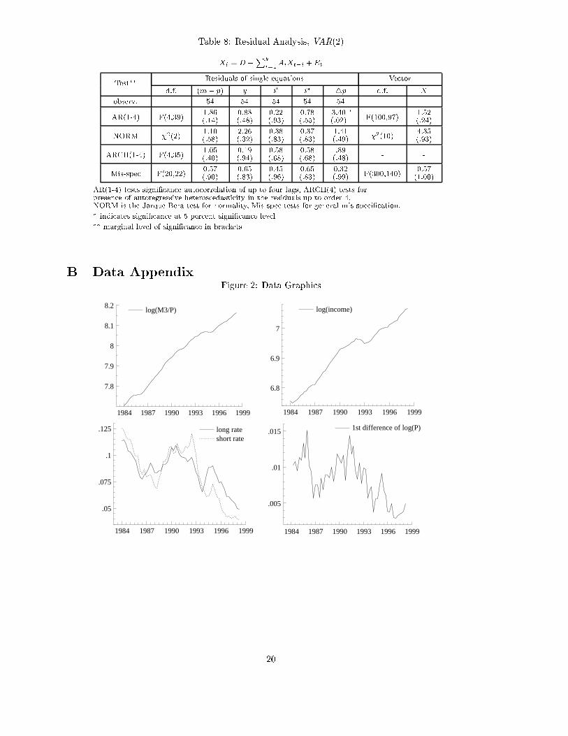
Table 8: Residual Analysis, VAR(2)

Xt = D +P

k

i=1AiXt�i +Et

Test��Residuals of single equations Vector

d.f. (m � p) y il is 4p d.f. X

observ. - 54 54 54 54 54 - -

AR(1-4) F(4,39)1:86(:14)

0:88(:48)

0:22(:93)

0:78(:55)

3:40(:02)

�

F(100,97)1:52(:24)

NORM �2(2)1:10(:58)

2:26(:32)

0:38(:83)

0:37(:83)

1:41(:49) �2(10)

4:35(:93)

ARCH(1-4) F(4,35)1:05(:40)

0:19(:94)

0:58(:68)

0:58(:68)

:89(:48) - -

Mis-spec F(20,22)0:57(:90)

0:65(:83)

0:45(:96)

0:65(:83)

0:32(:99) F(300,140)

0:57(1:00)

AR(1-4) tests signi�cance autocorrelation of up to four lags, ARCH(4) tests forpresence of autoregressive heteroscedasticity in the residuals up to order 4,NORM is the Jarque-Bera test for normality, Mis-spec tests for general mis-speci�cation.� indicates signi�cance at 5 percent signi�cance level�� marginal level of signi�cance in brackets

B Data AppendixFigure 2: Data Graphics

1984 1987 1990 1993 1996 1999

7.8

7.9

8

8.1

8.2log(M3/P)

1984 1987 1990 1993 1996 1999

6.8

6.9

7

log(income)

1984 1987 1990 1993 1996 1999

.05

.075

.1

.125 long rateshort rate

1984 1987 1990 1993 1996 1999

.005

.01

.015 1st difference of log(P)

20

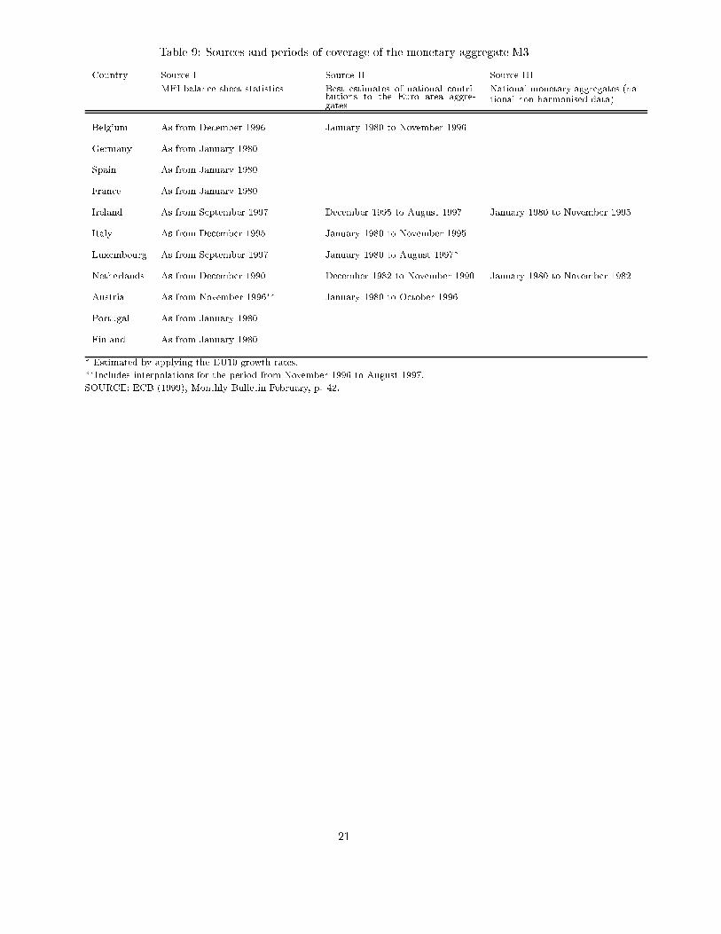
Table 9: Sources and periods of coverage of the monetary aggregate M3

Country Source I Source II Source III

MFI balance sheet statistics Best estimates of national contri-butions to the Euro area aggre-gates

National monetary aggregates (na-tional non-harmonised data)

Belgium As from December 1996 January 1980 to November 1996

Germany As from January 1980

Spain As from January 1980

France As from January 1980

Ireland As from September 1997 December 1995 to August 1997 January 1980 to November 1995

Italy As from December 1995 January 1980 to November 1995

Luxembourg As from September 1997 January 1980 to August 1997�

Netherlands As from December 1990 December 1982 to November 1990 January 1980 to November 1982

Austria As from November 1996�� January 1980 to October 1996

Portugal As from January 1980

Finland As from January 1980

� Estimated by applying the EU10 growth rates.��Includes interpolations for the period from November 1996 to August 1997.

SOURCE: ECB (1999), Monthly Bulletin February, p. 42.

21

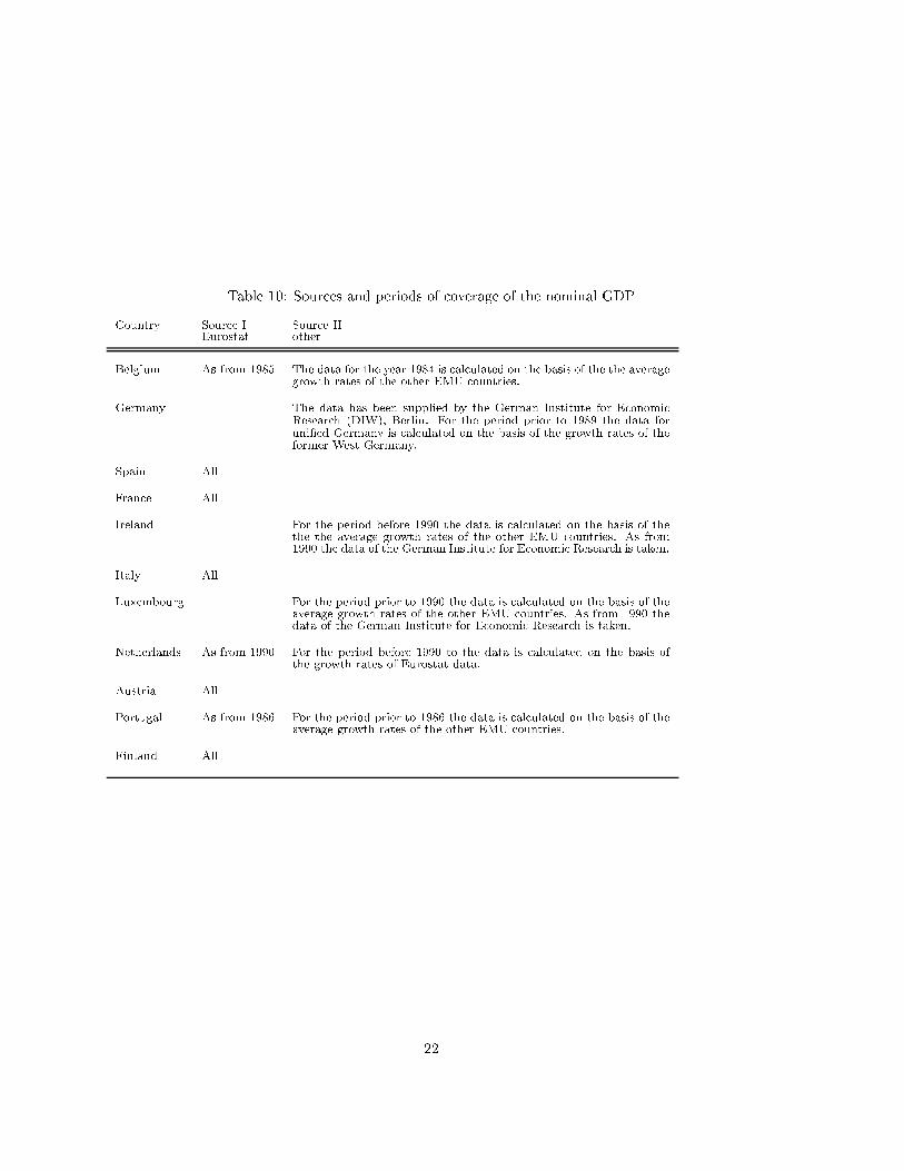
Table 10: Sources and periods of coverage of the nominal GDP

Country Source I Source IIEurostat other

Belgium As from 1985 The data for the year 1984 is calculated on the basis of the the averagegrowth rates of the other EMU countries.

Germany The data has been supplied by the German Institute for EconomicResearch (DIW), Berlin. For the period prior to 1989 the data foruni�ed Germany is calculated on the basis of the growth rates of theformer West Germany.

Spain All

France All

Ireland For the period before 1990 the data is calculated on the basis of thethe the average growth rates of the other EMU countries. As from1990 the data of the German Institute for Economic Research is taken.

Italy All

Luxembourg For the period prior to 1990 the data is calculated on the basis of theaverage growth rates of the other EMU countries. As from 1990 thedata of the German Institute for Economic Research is taken.

Netherlands As from 1990 For the period before 1990 to the data is calculated on the basis ofthe growth rates of Eurostat data.

Austria All

Portugal As from 1986 For the period prior to 1986 the data is calculated on the basis of theaverage growth rates of the other EMU countries.

Finland All

22

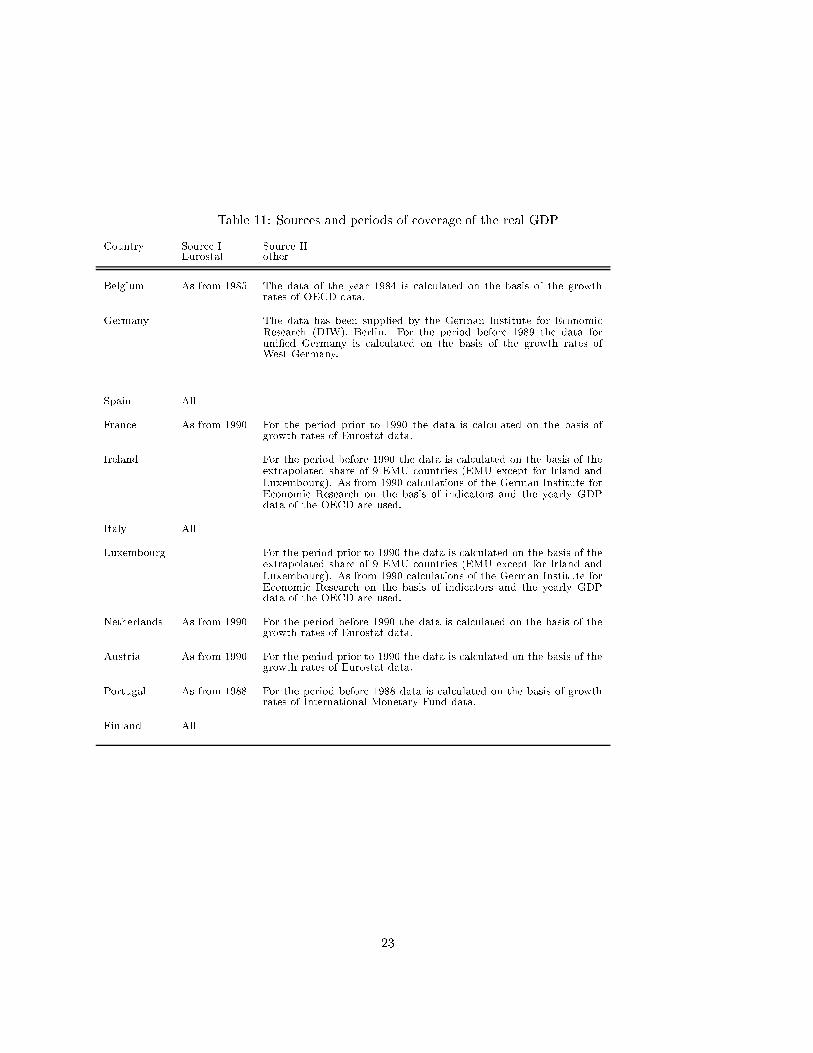
Table 11: Sources and periods of coverage of the real GDP

Country Source I Source IIEurostat other

Belgium As from 1985 The data of the year 1984 is calculated on the basis of the growthrates of OECD data.

Germany The data has been supplied by the German Institute for EconomicResearch (DIW), Berlin. For the period before 1989 the data foruni�ed Germany is calculated on the basis of the growth rates ofWest Germany.

Spain All

France As from 1990 For the period prior to 1990 the data is calculated on the basis ofgrowth rates of Eurostat data.

Ireland For the period before 1990 the data is calculated on the basis of theextrapolated share of 9 EMU countries (EMU except for Irland andLuxembourg). As from 1990 calculations of the German Institute forEconomic Research on the basis of indicators and the yearly GDPdata of the OECD are used.

Italy All

Luxembourg For the period prior to 1990 the data is calculated on the basis of theextrapolated share of 9 EMU countries (EMU except for Irland andLuxembourg). As from 1990 calculations of the German Institute forEconomic Research on the basis of indicators and the yearly GDPdata of the OECD are used.

Netherlands As from 1990 For the period before 1990 the data is calculated on the basis of thegrowth rates of Eurostat data.

Austria As from 1990 For the period prior to 1990 the data is calculated on the basis of thegrowth rates of Eurostat data.

Portugal As from 1988 For the period before 1988 data is calculated on the basis of growthrates of International Monetary Fund data.

Finland All

23

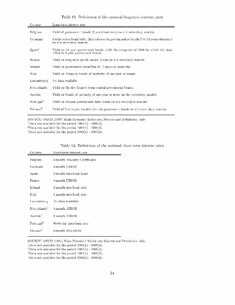
Table 12: De�nitions of the national long-term interest rates

Country Long-term interest rate

Belgium Yield of government bonds (6-years and over) on the secondary market.

Germany Public sector bond yield, that refers to long-term public bonds (7 to 15 years duration)on the secondary market.

Spain1 Yield on 10 year government bonds, with the exception of 1994 for which the datarefers to 9 year government bonds.

France Yield on long term public sector bonds on the secondary market.

Ireland Yield on government securities of 15 years to maturity.

Italy Yield on Treasury bonds of maturity of one year or longer.

Luxembourg No data available.

Netherlands Yield on the �ve longest term central government bonds.

Austria Yield on bonds of maturity of one year or more on the secondary market.

Portugal2 Yield on 10-year government debt bonds on the secondary market.

Finland3 Yield of 3 to 6 year taxable central government bonds on the secondary market.

SOURCE: OECD (1997) Main Economic Indicators, Sources and De�nitions, July.1Data not available for the period 1984(1) - 1986(4).2Data not available for the period 1984(1) - 1994(4).3Data not available for the period 1984(1) - 1987(4).

Table 13: De�nitions of the national short term interest rates

Country Short-term interest rate

Belgium 3-month Treasury Certi�cates

Germany 3-month FIBOR

Spain 3-month interbank loans

France 3-month PIBOR

Ireland 3-month interbank rate

Italy 3-month interbank rate

Luxembourg No data available.

Netherlands1 3-month AIBOR

Austria2 3-month VIBOR

Portugal3 86-96 day interbank rate

Finland4 3-month HELIBOR

SOURCE: OECD (1997) Main Economic Indicators, Sources and De�nitions, July.1Data not available for the period 1984(1) - 1985(4).2Data not available for the period 1984(1) - 1988(4).3Data not available for the period 1984(1) - 1985(2).4Data not available for the period 1984(1) - 1986(4).

24